Embed Size (px)
Citation preview
Systematic Prediction and Parametric Characterization of Thermo-AcousticInstabilities in Premixed Gas Turbine Combustors
Christopher Reed Martin
Thesis submitted to the faculty of the Virginia Polytechnic Institute and State University inpartial fulfillment of the requirements for the degree of
Master of Sciencein
Mechanical Engineering
Dr. William Baumann, Co-Chair,Dr. Uri Vandsburger, Co-Chair,
Dr. Robert West
September 29th, 2006Blacksburg, VA
Keywords:Thermo-Acoustic, Instability, Dynamic, Flame, Combustor
c©2006, Christopher R. Martin, All Rights Reserved

Systematic Prediction and Parametric Characterization of Thermo-Acoustic
Instabilities in Premixed Gas Turbine Combustors.
Christopher Reed Martin
ABSTRACT.
This thesis describes the coincident prediction and observation of thermo-acoustic instabilities ina turbulent, swirl-stabilized research combustor using a stability model constructed from validatedreduced-order component models. The component models included the acoustic response to flameheat release rate at various locations in the combustor, the turbulent diffusion of uneven fuel-airmixing, and the flame’s response to perturbations in both inlet velocity and equivalence ratio. Theseelements are closed in a system-level model to reflect their natural dynamic coupling and assessedwith linear stability criteria. The results include the empirical validation of each of the componentmodels and limited validation of the total closed-loop model with a lean premixed gaseous fuelcombustor not dissimilar to an industrial burner. The degree of agreement between the predictionsand the measurements encourages the conclusion that the reduced-order technique described hereinnot only includes the relevant physics, but has characterized them with sufficient acuracy to be thebasis for design techniques for the passive avoidance of thermo-acoustic instabilities.

iii
This work is dedicated to the loving memory ofSylvan J. Carrier
and to the spirit of restless persceverence he personified,

iv
and was funded by the United States Department of Energy.Many thanks to my benefactors for their contributions and their patience.
The author may be reachedBefore 2008: Christopher R. Martin
203A Randolph HallVirginia TechBlacksburg, VA 24061-0238(540)[email protected]
2009 and Thereafter: [email protected]
v
To my colleagues of the VACCG, to all those who taughtme and bore my questions and my impatience, and to theundernamed professors to name only a few, I owe a greatdebt.
William BaumannMark CramerMark PaulWilliam SaundersUri VandsburgerRobert West
Thank you.
CONTENTS
1. Introduction . . . . . . . . . . . . . . . . . . . . . . . . . . . . . . . . . . . . . . . . . . . . 11.1 Background . . . . . . . . . . . . . . . . . . . . . . . . . . . . . . . . . . . . . . . . . 21.2 Objectives and Scope . . . . . . . . . . . . . . . . . . . . . . . . . . . . . . . . . . . . 81.3 Methodology . . . . . . . . . . . . . . . . . . . . . . . . . . . . . . . . . . . . . . . . 9
2. The Dynamic Flame . . . . . . . . . . . . . . . . . . . . . . . . . . . . . . . . . . . . . . . 122.1 Decoupled Flame Model . . . . . . . . . . . . . . . . . . . . . . . . . . . . . . . . . . 122.2 General Integral Equations for a Reacting Flow . . . . . . . . . . . . . . . . . . . . . 142.3 Formulation of the Well-Stirred Reactor . . . . . . . . . . . . . . . . . . . . . . . . . 182.4 Chemical Kinetics . . . . . . . . . . . . . . . . . . . . . . . . . . . . . . . . . . . . . 232.5 Analysis by Perturbations . . . . . . . . . . . . . . . . . . . . . . . . . . . . . . . . . 292.6 The Physical Dynamic Flame . . . . . . . . . . . . . . . . . . . . . . . . . . . . . . . 332.7 Steady Solution of the Well-Stirred Reactor . . . . . . . . . . . . . . . . . . . . . . . 392.8 Bandwidth and Frequency Response . . . . . . . . . . . . . . . . . . . . . . . . . . . 462.9 Flame Transfer Function . . . . . . . . . . . . . . . . . . . . . . . . . . . . . . . . . . 58
3. Dynamic Turbulent Mixing . . . . . . . . . . . . . . . . . . . . . . . . . . . . . . . . . . . 603.1 Stochastic Mixing . . . . . . . . . . . . . . . . . . . . . . . . . . . . . . . . . . . . . . 613.2 The Random Walk and Diffusivity . . . . . . . . . . . . . . . . . . . . . . . . . . . . 623.3 Mixing Frequency Response . . . . . . . . . . . . . . . . . . . . . . . . . . . . . . . . 643.4 Validation . . . . . . . . . . . . . . . . . . . . . . . . . . . . . . . . . . . . . . . . . . 683.5 Establishing the Proper Units . . . . . . . . . . . . . . . . . . . . . . . . . . . . . . . 69
4. Acoustics . . . . . . . . . . . . . . . . . . . . . . . . . . . . . . . . . . . . . . . . . . . . . 73
5. System-Level Stability Predictions . . . . . . . . . . . . . . . . . . . . . . . . . . . . . . . 775.1 Classical Thermo-Acoustic Stability . . . . . . . . . . . . . . . . . . . . . . . . . . . 775.2 Assessing Stability . . . . . . . . . . . . . . . . . . . . . . . . . . . . . . . . . . . . . 795.3 Stability Characteristics . . . . . . . . . . . . . . . . . . . . . . . . . . . . . . . . . . 835.4 Closed-Loop Model Validation . . . . . . . . . . . . . . . . . . . . . . . . . . . . . . 93
6. Conclusions . . . . . . . . . . . . . . . . . . . . . . . . . . . . . . . . . . . . . . . . . . . . 96
LIST OF FIGURES
1.1 A cross-section of Trevelyan’s Rocker . . . . . . . . . . . . . . . . . . . . . . . . . . . 31.2 The Glass Blower’s Tube . . . . . . . . . . . . . . . . . . . . . . . . . . . . . . . . . . 41.3 A conceptual combustor burning premixed fuel-air . . . . . . . . . . . . . . . . . . . 101.4 System-Level Breakdown. Signals u′
inj, u′
flame, q, and Φ′ refer to the acoustic velocityat the injector, acoustic velocity at the flame, heat release rate, and equivalence ratioat the flame respectively. . . . . . . . . . . . . . . . . . . . . . . . . . . . . . . . . . . 11
2.1 An arbitrary region in a one-dimensional flow . . . . . . . . . . . . . . . . . . . . . . 182.2 Methane heat release rate response to velocity perturbations. (Ranalli) . . . . . . . . 362.3 Methane heat release rate response to equivalence ratio perturbations. (Ranalli) . . 362.4 Propane heat release rate response to velocity perturbations. (Ranalli) . . . . . . . . 372.5 Propane heat release rate response to velocity perturbations. (Ranalli) . . . . . . . . 372.6 Dynamic data summary: DC Gains. (Ranalli) . . . . . . . . . . . . . . . . . . . . . . 382.7 Dynamic data summary: Bandwidths. (Ranalli) . . . . . . . . . . . . . . . . . . . . 382.8 WSR temperature bifurcation diagram. Equilibria temperatures are plotted against
Φ and σ. Lines of constant Φ are in black and lines of constant σ are in blue. . . . . 422.9 Blowoff and σ = 0 conditions plotted against Φ. Blowoff is computed from Equation
2.46. . . . . . . . . . . . . . . . . . . . . . . . . . . . . . . . . . . . . . . . . . . . . . 432.10 WSR heat release rate bifurcation diagram. Equilibria heat release rates are plotted
against Φ and σ. Lines of constant Φ are in black and lines of constant σ are in blue. 442.11 WSR temperature and heat release rate bifurcation diagrams with lines of constant
σ and lines of constant Φ. . . . . . . . . . . . . . . . . . . . . . . . . . . . . . . . . . 472.12 Flame DC gains plotted against the non-dimensionalized steady system parameters.
σ has simply been scaled so that 1 corresponds to blowoff, while Φ has been scaledand shifted so that 0 is lean blowoff and 1 is an equivalence ratio of 1. . . . . . . . . 48
2.13 Heat release rate frequency response functions for a constant-mass reactor. . . . . . 552.14 Heat release rate frequency response functions for a constant-volume reactor. . . . . 552.15 Critical Exhaust Constraint cutoff frequency prediction as a function of equivalence
ratio. . . . . . . . . . . . . . . . . . . . . . . . . . . . . . . . . . . . . . . . . . . . . . 562.16 Heat release rate frequency response functions for a critical-exhaust-constrained re-
actor. . . . . . . . . . . . . . . . . . . . . . . . . . . . . . . . . . . . . . . . . . . . . 572.17 Root loci for the dynamic WSR (zeros omitted). The low-frequency coincident poles
correspond to the time-constant dynamics exhibited by the well-mixed tank. Thevarious size constraints place zeros in different places where they may or may notcancel with these poles. . . . . . . . . . . . . . . . . . . . . . . . . . . . . . . . . . . 58

List of Figures viii
2.18 Frequency response for the dynamic WSR with various arbitrary mass dependencies.(a) ∂M
∂Yf> 0, ∂M
∂Yox< 0
(b) ∂M∂Yf
> 0,
(c) ∂M∂T
< 0 . . . . . . . . . . . . . . . . . . . . . . . . . . . . . . . . . . . . . . . . . 59
3.1 A conceptual combustor burning premixed fuel-air. Repeated from Figure 1.3. . . . 603.2 Fuel concentration in mol/m plotted over normalized position for three points in
time with arbitrary values of U , v2, and xi. . . . . . . . . . . . . . . . . . . . . . . . 653.3 The mixing impulse response at the dump plane in mol/m with arbitrary values of
U , v2, and xi. . . . . . . . . . . . . . . . . . . . . . . . . . . . . . . . . . . . . . . . . 663.4 The mixing frequency response computed from Figure 3.3. . . . . . . . . . . . . . . . 673.5 Mixing transfer function cutoff frequency as a function of the σt estimate in Equation
3.10 . . . . . . . . . . . . . . . . . . . . . . . . . . . . . . . . . . . . . . . . . . . . . 693.6 Predicted mixing transfer function plotted against the measured transfer function at
two points in space. . . . . . . . . . . . . . . . . . . . . . . . . . . . . . . . . . . . . 703.7 System diagram of the mixing elements. M ′ is the transfer function from the injection
function, s, to the fuel concentration at the dump plane determined above. . . . . . 72
4.1 A conceptual combustor burning premixed fuel-air. Repeated from Figure 1.3 . . . . 734.2 Original, open-to-atmosphere combustor acoustics. Magnitude units are in m/J .
Plot (a) represents the response at the dump plane and (b) represents the responseat the injection plane. . . . . . . . . . . . . . . . . . . . . . . . . . . . . . . . . . . . 75
4.3 Modified, lengthened combustor acoustics. Magnitude units are in m/J . Plot (a)represents the response at the dump plane and (b) represents the response at theinjection plane. . . . . . . . . . . . . . . . . . . . . . . . . . . . . . . . . . . . . . . . 76
5.1 System-Level Breakdown with a hypothetical disturbance. Signals uinj , uflame, q,
and Φ refer to the acoustic velocity at the injector, acoustic velocity at the flame,heat release rate, and equivalence ratio at the flame respectively. Am, AΦ, Fm, FΦ,and M refer to the acoustic transfer functions at the combustor dump and injector,flame response to velocity perturbations, and the mixing transfer function respectively 81
5.2 Km plotted against σ for various values of Φ. Repeated from Figure 2.12. . . . . . . 845.3 The mass-flow coupling OLTF plotted for various Φ and σ values. Phase crossings
are marked with vertical lines. Plots (a) and (b) are both very close to blowoff. Plots(c) and (d) are at various locations well inside the flame operating envelope. . . . . . 86
5.4 Stability error plotted against σ for Φ = 0.70 for a system with mass flow couplingonly. . . . . . . . . . . . . . . . . . . . . . . . . . . . . . . . . . . . . . . . . . . . . . 87
5.5 Stability error plotted against Φ and σ for a system with velocity coupling only. Zerointersects are highlighted with the bold lines. . . . . . . . . . . . . . . . . . . . . . . 87
5.6 Maximum gain ratio between open loop transfer functions for the mass flow couplingand the mixing coupling . . . . . . . . . . . . . . . . . . . . . . . . . . . . . . . . . . 88
5.7 The OLTF with both mass flow and mixing couplings plotted for various Φ and σvalues. Phase crossings are marked with vertical lines. . . . . . . . . . . . . . . . . . 89
5.8 Open-Loop Transfer Function for the mixing transfer function (KFΦAΦM). . . . . . 905.9 Km and KΦ plotted against Φ for various values of σ. Repeated from figure 2.12 . . 91
List of Figures ix
5.10 Stability error plotted against σ for Φ = 0.50 for a system with both mass flow andmixing coupling. . . . . . . . . . . . . . . . . . . . . . . . . . . . . . . . . . . . . . . 91
5.11 Stability error plotted again Φ and σ for a system with both velocity and mixingcoupling. Zero intersects are highlighted with the bold lines. . . . . . . . . . . . . . . 92
5.12 Critical combustor stability predictions with mass-flow perturbations only, mixingperturbations, and mixing perturbations only. There is a mass-flow instability ex-tremely close to blowoff, obscured by proximity to the black blowoff curve. . . . . . . 93
5.13 Stability Validation . . . . . . . . . . . . . . . . . . . . . . . . . . . . . . . . . . . . . 95
1. INTRODUCTION
Thermo-acoustic combustion instabilities occur when a flame and the acoustics in the surrounding
fluid couple dynamically to form a self-exciting, linearly unstable system. Though study into
the nature of these instabilities is well-motivated by the destructive power of the resulting acoustic
oscillations alone without even including mention of the cost incurred in the gas turbine industry due
to reduced combustion efficiency or poorer emissions[9], detailed studies[22] of such instabilities have
been inhibited by the formidable challenge inherent to understanding and characterizing dynamic
reacting flows. To add to these complexities, the importance of the surrounding acoustics invites
dependencies on combustor geometry, fuel type, injection method, etc. . . , each of which varies even
within a fleet of engines. It is the unfortunate result that even in the face of steady advances in
modeling techniques to capture these phenomena, much industrial design is still mostly restricted
to be based on empirical knowledge.
Gas turbine combustion is often classified by fuel types (liquid or gaseous), but this can be
a misleading distinction since premixed, prevaporized liquid fuel can behave very much like pre-
mixed gaseous fuel. It is more convenient for the purpose of investigating instabilities, therefore,
to consider premixed and direct injection combustors as distinct. Direct injection combustors,
depending upon the application, either rely upon very rapid mixing (and vaporization if liquid
fueled) to produce a semi-homogeneous mixture prior to combustion, or form a diffusion flame at
the fuel-air interface. Premixed combustion, on the other hand, allows the fuel time to mix (and
vaporize if necessary) with the air prior to combustion. Each of these systems presents distinct
physical phenomena that are extremely difficult to capture in a single model. To name only sev-
eral of the challenges such a model would have to surmount, diffusion flames take on completely
different geometries than premixed flames, and the different mixing methods provide means for
1. Introduction 2
acoustic-mixing interactions that are entirely unique to the different injection geometries.
This particular work is designed to develop a systems-based approach to predicting the forma-
tion of thermo-acoustic instabilities that might eventually be systematically applied to premixed
combustors (and potentially even LDI combustors) of various geometries prior to obtaining direct
empirical measurements. By identifying the significant physical elements of a thermo-acoustic in-
stability in a lean, premixed gas turbine combustor, it is possible that linearized system elements
can be closed analytically to allow predictions on closed-loop stability. Such models are of interest
to both academic and industrial communities, since not only do predictive models provide invalu-
able influence in the design of new products and the modification of existing ones, but, as this
discussion will show, can also provide unique insights into the physical phenomena that cause these
instabilities.
1.1 Background
Thermo-acoustic phenomena were first noted by Higgins in 1777 in the form of a “singing flame”[26].
Later, some of the earliest records of scientific investigation into thermo-acoustic instabilities were
cataloged in Lord Rayleigh’s The Theory of Sound [23], originally published in 1877. The thermally
driven oscillations he listed therein included four distinct phenomena: a thermo-mechanical insta-
bility called Trevelyan’s Rocker, a thermo-acoustic instability that shall be named in this document
as Chladni’s Tube for the acoustician that Rayleigh credited for its discovery, singing that occurs
naturally in a Glassblower’s Tube, and the much celebrated thermo-acoustic instability that occurs
in Rijke’s Tube.
Trevelyan’s Rocker
An interesting distraction from thermo-acoustic oscillations, this is an indication of the potentially
counter-intuitive nature of thermally-driven instabilities. Frequently, as in the case of Trevelyan’s
Rocker, since the instability results in large-scale oscillations, one is reluctant to investigate the
physics of smaller scales to seek an explanation, though that may actually be where the explanation
lies.

1. Introduction 3
� �B
BBB
BB
������
Fig. 1.1: A cross-section of Trevelyan’s Rocker
Trevelyan’s Rocker is a hot, metallic isosceles triangular prism with a trench cut in place of the
a-symmetric angle, the cross-section of which appears in Figure 1.1. When the metal was heated
and placed on a cool lead surface, the device emitted an audible tone. It has subsequently been
noted that the pitch is due to rapid rocking oscillations - hence the device’s name. It is sufficient to
note that there was significant debate as to the cause of the oscillations, the most widely accepted
explanation being that alternating thermal expansion and contraction of the lead drove a self-
sustaining rocking motion in the prism. Objections to this explanation included that the time-scale
associated with transient heating and cooling are much slower than would be necessary to keep up
with the frequencies of oscillation observed.
Though discussion on the nature of these oscillations persists, Bhargava and Ghosh[1] have
treated the matter with a very simple derivation that agrees sufficiently with empirical observations
as to encourage the conclusion. Ultimately, the objections were refuted by noting that when only
the local heating and cooling at the very small points of contact need be considered, the time scale
for thermal decay becomes significantly faster. The lesson to be learned from this endeavor is that
these dynamic phenomena defy many of the constructs and intuitions developed around slow or
semi-steady phenomena. For this reason it is important to re-investigate many of the preconceived
notions surrounding even well-understood phenomena.
Glass Blower’s Tube
Of the thermo-acoustic instabilities discussed in Rayleigh’s book, the relevant physics in the Glass
Blower’s Tube are the simplest. So, it is with good reason that it is the first of the thermo-acoustic
systems to be discussed. This example offers the first glimpse into the physical principles that will
remain relevant from one instance of thermo-acoustic coupling to another.
1. Introduction 4
� �� �
� �� �Workpiece
Hot
Cold
Fig. 1.2: The Glass Blower’s Tube
Glass blowers traditionally use a long hollow rod to thrust the work piece into a furnace where
the glass is heated until it becomes malleable. The artist blows through the hollow rod to inflate
the glass shape into a hollow container. Clearly, the artist is reliant upon the thermal insulation
along the length of the rod to maintain a safe temperature at the mouthpiece. Interest among
the acoustic community was turned to these devices when glassblowers noticed an audible tone
emanating from unattended tubes under some conditions.
Figure 1.2 shows a crude representation of the physical system. The oscillations are caused by
unsteady heat transfer to and from the air as it expands and contracts in the tube. At semi-steady-
state, any heat transfer from the workpiece to the air inside causes an expansion. As the slightly
hotter air expands into the tube, the heat is given up to the cooler walls of the tube, causing a
contraction, after which the process is repeated. The phenomenon is, in fact, a naturally occurring
heat engine that extracts energy in the form of acoustic oscillations rather than shaft work.
Rijke’s Tube
Perhaps the most famous of the examples included in Rayleigh’s survey of thermally-driven in-
stabilities due to its perceived similitude to the instabilities noted in modern gas turbine en-
gines, Rijke’s tube is a favorite for classroom demonstrations and simplified modern stability
experiments[6, 13, 16].
The Dutch physicist Pieter Rijke noted that by inserting a heated metallic gauze in an open
vertical tube 1/4 the tube’s length from the bottom, the emission of a strong tone is audible[23].
The hot gauze transfers heat to the surrounding air, driving a steady current through the tube due
to the buoyancy of the heated air. Any slight accelerations in the air velocity cause improved heat
transfer, ultimately resulting in enhanced heat addition to the air. Similarly, retarded air velocity

1. Introduction 5
deters heat transfer and results in a decline in heat addition. In this manner there is a natural
coupling between the acoustics in the tube and the addition of heat to the air in the tube.
Surely one of the primary reasons Rijke’s experiment is so popular as an academic curiosity is
found in the realization that the phase of the acoustic cycle at which heat is added can be easily
adjusted with the vertical position of the gauze in the tube. Thus, it is a simple matter to observe
physical limits on stability simply by adjusting the gauze location in the tube.
Chladni’s Tube
Though it is rarely (if ever) mentioned in the modern combustion literature, Chladni’s tube is
more relevant to gas turbine thermo-acoustic instabilities than any of the other classic examples
in the literature. While both the glassblower’s tube and Rijke’s tube are thermo-acoustic systems
driven by unsteady heat transfer and Trevelyan’s rocker is driven by thermo-mechanical coupling,
Chladni’s tube is unique in the sense that it alone exhibits an instability driven by a flame.
An acoustician famous for his experiments identifying mode-shapes in vibrating plates with
pooling particulates, Chladni is credited as noting (though Higgins is recorded as first noting
a similar phenomenon) that a hydrogen flame in a tube produced a pitch similar to the other
instabilities. Other experimenters noted that the oscillation could be suppressed by damping the
propagation of acoustic waves through the tube supplying the fuel with cotton, while parameters
such as the fuel line’s length and diameter seemed to matter less. This encouraged what is now
a common conclusion: that the propagation of unsteady fuel injection into the flame can drive a
thermo-acoustic instability.
Rayleigh Criterion for Stability
With regard to these phenomena, in 1878 Sir Rayleigh published both in The Proceedings of the
Royal Institute and Nature, these words which have become the basis for a number of mathematical
criteria for thermo-acoustic stability posed since:
“If heat be periodically communicated to, and abstracted from, a mass of air vibrating
(for example) in a cylinder bounded by a piston, the effect produced will depend upon
1. Introduction 6
the phase of the vibration at which the transfer of heat takes place. If heat be given to
the air at the moment of greatest condensation, or be taken from it at the moment of
greatest rarefaction, the vibration is encouraged. On the other hand, if heat be given
at the moment of greatest rarefaction, or abstracted at the moment of greatest con-
densation, the vibration is discouraged. The latter effect takes place of itself when the
rapidity of alternation is neither very great nor very small in consequence of radiation;
for when air is condensed it becomes hotter, and communicates heat to surrounding
bodies. The two extreme cases are exceptional, though for different reasons. In the
first, which corresponds to the suppositions of Laplace’s theory of the propagation of
sound, there is not sufficient time for a sensible transfer to be effected. IN the second,
the temperature remains nearly constant, and the loss of heat occurs during the process
of condensation, and not when the condensation is effected. This case corresponds to
Newton’s theory of the velocity of sound. When the transfer of heat takes place at the
moment of greatest condensation or of greatest rarefaction, the pitch is not affected.
If the air be at its normal density at the moment when the transfer of heat takes place,
the vibration is neither encouraged nor discouraged, but the pitch is altered. Thus the
pitch is raised if the heat be communicated to the air a quarter period before the phase
of greatest condensation; and the pitch is lowered if the heat be communicated a quarter
period after the phase of greatest condensation.
In general both kinds of effects are produced by periodic transfer of heat. The pitch is
altered, and the vibrations are either encouraged or discouraged. But there is no effect
of the second kind if the air concerned be at a loop, i.e. a place where the density does
not vary, nor if the communication of heat be the same at any stage of rarefaction as
at the corresponding stage of condensation.”[23]
The first realization of a mathematical criterion for instability, similar in principle to Rayleigh’s
qualitative description, is typically credited to Putnam in his study of Combustion-Driven Oscilla-
tions in Industry [22] and his earlier Survey of Organ-Pipe Oscillations in Combustion Systems[21].
1. Introduction 7
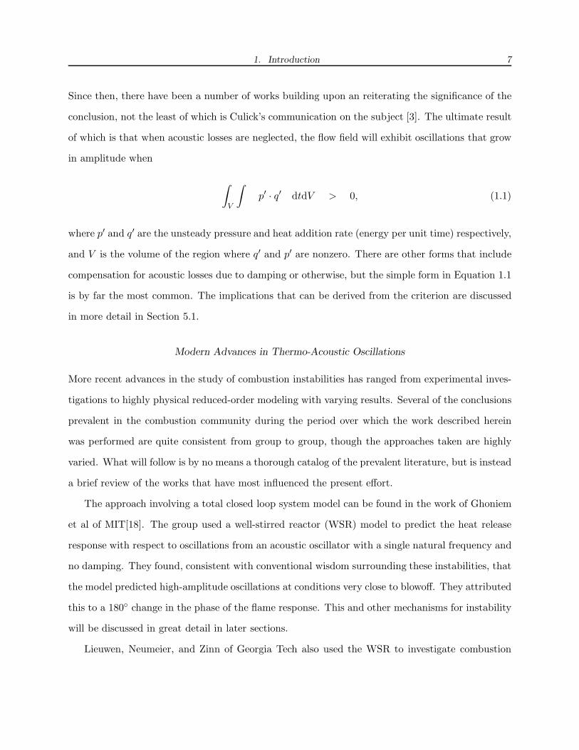
Since then, there have been a number of works building upon an reiterating the significance of the
conclusion, not the least of which is Culick’s communication on the subject [3]. The ultimate result
of which is that when acoustic losses are neglected, the flow field will exhibit oscillations that grow
in amplitude when
∫
V
∫p′ · q′ dtdV > 0, (1.1)
where p′ and q′ are the unsteady pressure and heat addition rate (energy per unit time) respectively,
and V is the volume of the region where q′ and p′ are nonzero. There are other forms that include
compensation for acoustic losses due to damping or otherwise, but the simple form in Equation 1.1
is by far the most common. The implications that can be derived from the criterion are discussed
in more detail in Section 5.1.
Modern Advances in Thermo-Acoustic Oscillations
More recent advances in the study of combustion instabilities has ranged from experimental inves-
tigations to highly physical reduced-order modeling with varying results. Several of the conclusions
prevalent in the combustion community during the period over which the work described herein
was performed are quite consistent from group to group, though the approaches taken are highly
varied. What will follow is by no means a thorough catalog of the prevalent literature, but is instead
a brief review of the works that have most influenced the present effort.
The approach involving a total closed loop system model can be found in the work of Ghoniem
et al of MIT[18]. The group used a well-stirred reactor (WSR) model to predict the heat release
response with respect to oscillations from an acoustic oscillator with a single natural frequency and
no damping. They found, consistent with conventional wisdom surrounding these instabilities, that
the model predicted high-amplitude oscillations at conditions very close to blowoff. They attributed
this to a 180◦ change in the phase of the flame response. This and other mechanisms for instability
will be discussed in great detail in later sections.
Lieuwen, Neumeier, and Zinn of Georgia Tech also used the WSR to investigate combustion
1. Introduction 8
oscillations. They postulated that not only perturbations in the fluid velocity local to the flame,
but also fluctuations in the equivalence ratio due to uneven fuel-air mixing can cause oscillations
in the heat release rate[10, 11]. They were able to show that the WSR predicts significant heat
release rate oscillations with respect to both velocity and mixing perturbations.
The same group has since abandoned the use of WSR’s to model dynamic combustion under
the premise that they predict unreasonable bandwidths. Their more recent publications have
included flame sheet models[19, 20], arguing that even turbulent flames behave as a flame sheet,
and implying that provided the local flame speed is conserved, the heat release rate is proportional
to the flame sheet area. The same has been applied by a number of researchers including Lawn
and Polifke[8] of the University of London and Die Technische Universitat Munchen respectively,
and Dowling[5] of The University of Cambridge. Lawn and Polifke adapted their model to be very
empirical in an attempt to match physical results. Similarly, Dowling presumed a flame geometry
based on observation and considered deviations from the steady case. What is consistent between
the works is the notion that the frequency response of the flame is scalable by the characteristic
time indicated by the flame length divided by the mean fluid velocity, L/U . This is a concept that
will be investigated in detail in the chapters to follow.
Lastly, but far from the least of these is the work of Lohrmann and Buchner who took experi-
mental measurements of a turbulent, swirl stabilized flame’s transfer function. They used a speaker
to drive unsteady flow into the flame and optically measured fluctuations in the heat release rate.
The significance of the work to the present effort demands that attention be paid to their findings.
In Chapter 2, their conclusions are compared at some length with the findings of this thesis.
1.2 Objectives and Scope
This work was originally conceived to address a growing need for systemically applicable methods
to predict and suppress thermo-acoustic combustion instabilities and has since grown in ambition to
address conditions under which the different mechanisms for instability become important. Herein,
I will describe my efforts to attain these goals by first dividing the complicated, nonlinear dynamic
system in a set of simpler, “system-level” component models, and finally their reconstruction into
1. Introduction 9
a total stability model.
The ultimate objective of developing design tools for the prediction of thermo-acoustic combus-
tion instabilities in lean, premixed gas turbine engines is divided into the following milestones:
1. The identification of dominant physical phenomena contributing to instability at various op-erating conditions,
2. Detailed description of the relative importance of the proposed mechanisms for instability,
3. The development of reduced-order mathematical models, applicable to practical systems, cap-turing the dominant dynamics,
4. and Detailed methods for closing the component models in a total closed-loop for the predictionof total stability.
The detail I devote to each model element is limited primarily by the novelties that are likely
to be found in each respective undertaking. For this reason, I have given great care to properly
developing theory surrounding the flame so that appropriate detail can be devoted to discussing
the perceived results and conjecturing the potential for future growth. Similarly, final closed-loop
analysis is developed in excellent detail as its results are the most unique of all.
The combustor acoustic models, however, despite their vital importance to determining the
closed-loop response, are allowed only limited description. This serves several purposes, prime
among them is to reserve credit for their conception for other researchers who developed them,
and also to prevent investigation into elements of the model that are known not to be immediately
portable to other systems. Indeed, the determination of detailed acoustic models is a potentially
cumbersome yet necessary undertaking for the construction of a total stability model that is worthy
of its own thesis. Therefore, the discussion herein with regard to acoustics shall be limited strictly
to that which is necessary to develop the total model.
1.3 Methodology
Flames in a given combustor geometry are sensitive to three parameters (dynamically and statically)
- pressure, equivalence ratio, and total mass flow entering the flame[25]. There is significant litera-
ture demonstrating that only large changes in pressure have significant effects on combustion[25, 7],

1. Introduction 10
-Air In
@@ @@ @@ @@ @@ @@ @@ @@ @@ @@ @@ @@ @@ @@ @@ @@ @@ @@ @@ @@
@@ @@ @@ @@ @@ @@ @@ @@ @@ @@ @@ @@ @@ @@ @@ @@ @@ @@ @@
Flame
-Dump Plane
-Exit Plane
?
Fuel In
Injection Plane
Fig. 1.3: A conceptual combustor burning premixed fuel-air
consistent with the work of Gohniem et al[18] and Lieuwen et al[11] whose flame models specifically
excluded pressure perturbations, citing them as insignificant relative to the effects observed from
mass flow and mixing excitations. It remains, therefore, to identify and model phenomena that can
potentially cause self-excited mass flow and equivalence ratio oscillations.
If a premixed combustor can be conceptualized as having geometry similar to Figure 1.3, then
it is immediately obvious that acoustic velocity perturbations at the dump plane result directly in
mass flow oscillations to the flame. Observe also that the equivalence ratio is determined entirely
by the ratio of local air velocity and fuel velocity at the injection plane. In combustors with choked
fuel flow or liquid fuel, it is quite common that pressure perturbations in the combustor have little
or no effect on the fuel mass flow at the injection plane, meaning that in such systems acoustically
driven velocity oscillations in the air flow at the injection plane will induce oscillations in the fuel-
air mixture. The actual effect on the equivalence ratio in the mixture delivered at the dump plane
is slightened by turbulent diffusion which occurs in the length of combustor between the injection
plane and the dump plane. Finally, all these processes that originate with acoustic oscillations in
the combustor and in turn excite the flame are potentially self-excited due to the natural coupling
that also exists between the flame’s heat release and the combustor acoustics.
Though there are well-established means for linearly estimating the acoustic physics, turbulent
mixing and the flame both include extremely nonlinear behaviors that pose a great challenge to
evaluating a realistic system response to anything but the most trivial of disturbance excitations.

1. Introduction 11
Acoustics (upstream)
6Acoustics (flame)
-
u′
dump
Flame (velocity)-�
��
�
�q
Flame (Φ)
?
Mixing
-
u′
inj
Φ′
Fig. 1.4: System-Level Breakdown. Signals u′
inj , u′
flame, q, and Φ′ refer to the acoustic velocity at the injec-tor, acoustic velocity at the flame, heat release rate, and equivalence ratio at the flame respectively.
There is no need to embark on the taxing process of nonlinear analysis, however. Note that so
long as any disturbance inputs are sufficiently small as to remain in the system’s linear range linear
stability alone will ensure that these disturbances decay. If this is indeed the case, only linearly
unstable systems will ever develop oscillations of significant amplitude.
Therefore, the component elements described above may be linearized about any desired oper-
ating conditions and closed to assess linear stability as in Figure 1.4. In this total model, the flame
and acoustics have each been sub-divided further into their relevance to the two loops - closure
with mixture perturbations, and closure with mass flow perturbations.
2. THE DYNAMIC FLAME
The decoupled flame model is responsible for mapping oscillating mass flows and equivalence ratios
to the oscillations in total heat release rate that drive acoustical phenomena. A variety of existing
flame models with varying sophistication illustrate in detail the physical phenomena that elicit
steady changes in the flame[7, 25], but it is another matter entirely, as evidenced by the persisting
academic discourse on the subject[18, 11, 19, 20, 14], to be certain of the physical processes that
influence the flame’s transient behavior. Though models with sufficient sophistication such as com-
putational fluid dynamical (CFD) models bypass the need for a conceptual grasp of the physics at
work by simply attempting to be all inclusive. Such models are often prohibitively computation-
ally intensive, geometry specific, and due to the tentative nature of computational models, there
even remains reasonable question as to the model’s accuracy. For these reasons, there is ample
motivation for the development of a reduced-order dynamic flame model.
In any effort to capture these physics mathematically, there is first to positively identify any
physical processes that are uniquely dynamic and that the existing steady models may have ne-
glected. Then, since these physics have been postulated to vary with operating conditions, com-
bustor and flame geometry, and fuel composition to mention only a few, it is essential to identify
the limits of any such model’s accuracy.
2.1 Decoupled Flame Model
It is worth noting that the flame model is not necessarily trivial to decouple from the surrounding
acoustics. This can be exemplified by considering a combustor with a reacting flow occupying its
entire length. In such a case, spatial variations brought about by standing waves are on the same
length scale (for even the longest wavelengths) as the flame length. In such a case, the conditions
2. The Dynamic Flame 13
encountered by the flame at all points in space will influence the local heat release, which will
in turn generate a local acoustic excitation. In this manner, reactions distributed throughout an
acoustic system are extremely inconvenient to divide into component parts.
The other extreme—a case in which the flame is a thin sheet with a face normal to the flow in
the combustor—presuming that a convenient 1-dimensional coordinate system is readily apparent,
only conditions at the single point along the combustor length at which the flame exists are needed
to determine the heat release. Similarly, the heat release is only acoustically coupled at the same
point in space, meaning only a finite set of scalars is necessary to completely define the flame’s
coupling with the rest of the dynamic system.
Reality is clearly neither of these cases, but some condition between them. It is simple enough
to assess to what extent the flame is inseparable from the acoustics by considering the flame length,
lf , and the acoustic wavelength, λn, corresponding to the wave number, n. If
lf � λn (2.1)
for the highest wave number exhibiting a significant amplitude, then reason would indicate it
possible to estimate the flame as a thin sheet whose internal structure is independent of acoustic
disturbances save those scalar parameters at the point in space where the flame is supposed to
exist.
Granted the abstraction that the flame’s internal structure is free of spatially dependent acoustic
effects, it is left only to determine the nature of that structure and what parameters—be they steady
or dynamic—are necessary to close the model. The highly turbulent flows that exist in virtually
all practical combustion systems induce excellent mixing, making most models based on laminar
phenomena wholly inappropriate. In fact, the improved mixing tends to trivialize any spatial
gradients in the flame, motivating Lieuwen et al[11], Ghoniem et al[18], and Losh[13] each to use
models that completely neglect all spatial variations in such flames.
Because of the advantageous simplifications such an assumption affords with little apparent
loss in applicability, this work will also begin by neglecting spatial variations in the flame, but
2. The Dynamic Flame 14
the assertion that the flame’s internal structure is so trivial is one that will be reassessed by this
chapter’s end. The models used by Ghoniem, Lieuwen, and Losh were all well-stirred reactors
(WSR) modified from their classical realization[7, 25] to include dynamic effects. Though the
extent to which various dynamics were eliminated or simplified varies in each of the works, the
fundamental rules governing the WSR are common to all.
1. The flame consists of a finite volume in space (called a reactor) in which chemical reactions
occur exclusively,
2. The contents of the reactor are sufficiently well mixed to neglect all spatial variation within
the reactor, allowing the contents to be described by scalar functions of time,
3. There are only two states necessary to describe the reactor - the inlet state (fluid entering
the reactor) and the internal state (since fluid leaving must necessarily be identical in state
to the internal fluid).
The following sections will develop the general reacting flow integral equations, adapt them to
describe a well-stirred reactor, adopt single-step chemical kinetics into the model, and investigate
to what extent the resulting equations reflect a realistic system by comparison with empirically
obtained dynamic flame data. It will be readily apparent that though the discussions in the afore
mentioned works are distinctly lacking on the topic, defining the arbitrary reactor volume is a very
delicate matter with strong implications on the resulting dynamics.
2.2 General Integral Equations for a Reacting Flow
If the reactor can be defined by some simply connected region in space it is convenient to describe
the region using integral equations by the method adopted by Panton[17]. Firstly, observe that the
mass of the region is defined by
M (t) =
∫∫∫
V (t)ρdV. (2.2)
2. The Dynamic Flame 15
Notice that since there is no constraint on the volume of the region, it must remain a function
of time, which shall be defined later. Similarly, the mass of the region is also a function of time.
In order to write the conservation equation in a familiar form, we may, with no loss of generality,
consider a material region - one whose surface has velocity equal to the local fluid velocity such
that the region contains a constant mass - that appears exactly coincident with the flame region.
The distinction is that though the reactor region is moving in a yet undetermined manner relative
to the fluid, a material region moves with the fluid, allowing constraints to be placed on the mass
and volume. Since the mass of such a region is constant,
0 =dMm
dt=
d
dt
∫∫∫
V (t)ρdV.
The subscript, m, indicates that the corresponding parameter refers to the material region. Using
Leibniz to commute the derivative into the integral,
0 =
∫∫∫
Vm(t)
∂ρ
∂tdV +
∫∫
Sm(t)ρ~u · ~dS, (2.3)
where Sm is the surface defining the material region, the vector, ~dS, is an outwardly pointing
differential surface area vector, and ~u is the fluid velocity.
Even though Equation 2.3 was derived by considering a material region and the WSR describes
an arbitrary region, it and other conservation equations still apply at all points in time. This
is true since though the material region and the reaction region move distinctly in space, it is
always possible to consider a material region that is exactly coincident with the reaction region
and to which Equation 2.3 applies. Along similar lines, since Equation 2.3 only need be considered
when the material region is coincident with the reaction region, it is unnecessary to distinguish the
material and reaction bounds of integration, allowing us to finally conclude that
0 =
∫∫∫
Vr(t)
∂ρ
∂tdV +
∫∫
Sr(t)ρ~u · ~dS, (2.4)
where the subscript, r refers to an arbitrary reaction region. Equation 2.4 gives an intuitive

2. The Dynamic Flame 16
relationship between the velocities entering and exiting the reaction region and the accumulation
of mass (density) inside the region. It will be shown in the next section that though this law is not
used directly to compute the reactor state, it is used to simplify other equations.
An equation of state governing the formation and destruction of species comes similarly from
considering the relation
Mi (t) =
∫∫∫
Vm(t)ρYidV, (2.5)
where the index, i, refers to the ith species, and Yi is the mass fraction of the same species. The
change in the mass of species i in a material region is related to the reaction rate of the same species
by
dMi
dt=
∫∫∫
Vm(t)ωidV. (2.6)
The rate of formation in mass per unit time per unit volume of species i, ωi, is calculated from
some set of chemical kinetic equations, which will be dealt with in Section 2.4, and may be taken
to be a function of the internal reaction region state only. Though the reaction rate equation will
undoubtedly introduce strong nonlinearities, the fact that it is only a function of the internal state
is an important simplification for the closure of the system. Differentiating Equation 2.5, applying
Leibniz’s rule as before, combining with Equation 2.6, and applying the same arbitrary change of
integration,
∫∫∫
Vr
ωidV =
∫∫∫
Vr
∂
∂t(ρYi) dV +
∫∫
Sr
ρYi~u · ~dS. (2.7)
Equation 2.7 can be rewritten to describe each species present in the mixture. Species that do not
participate in the chemical reaction (called a diluent), but that are present in the mixture, simply
have a zero reaction rate.
The last of the necessary conservation equations can be obtained by considering the first law of
2. The Dynamic Flame 17
thermodynamics applied to the same flame region as before.
d
dt
∫∫∫
Vm
eρdV = −∫∫
Sm
p~u · dS − Q (2.8)
The left-hand-side of Equation 2.8 is simply the time derivative of the total internal energy, ne-
glecting kinetic energy. The right-hand side includes work leaving the system neglecting viscous
and body forces, and heat transfer out of the region. Though the heat transfer is likely to be quite
a complicated function, like reaction rate, it will only be a function of the flame’s internal state.
This simplifies the problem of closure which will be dealt with in a later section. Using Leibniz’s
rule as before, applying the change of integration to an arbitrary region, and combining integrals
on like bounds
∫∫∫
Vr
∂
∂t(eρ) dV +
∫∫
Sr
ρ
(e +
p
ρ
)~u · dS = −Q.
Observe that the quantity appearing naturally in the surface integral is enthalpy. The fact that
enthalpy naturally takes into account both internal thermal energy and mechanical compressive
energy stored in a fluid allows the quantity to appear naturally in such derivations. It is a natural
choice to write the energy equation in terms of enthalpy since combustion properties are commonly
reported in terms of enthalpy. The appearance of internal energy alone in the volume integral is
inconvenient, but substitution of the definition of enthalpy (h ≡ e+p/ρ) can compltely eliminate the
last explicit dependence on e. The result is that the time derivative of pressure counter intuitively
appears as a source term.
∫∫∫
Vr
∂
∂t(hρ) dV +
∫∫
Sr
ρh~u · dS = −Q +
∫∫∫
Vr
∂p
∂tdV (2.9)
This concludes the fluid dynamical equations for a WSR. Momentum is absent since reactor
pressure need not be determined (nor can it be) exclusively by the WSR without knowledge of
the surrounding acoustics. The computation of the pressure and velocities in the reaction region
therefore must fall to a separate model. Similarly, there was no development of geometric constraints
2. The Dynamic Flame 18
- -
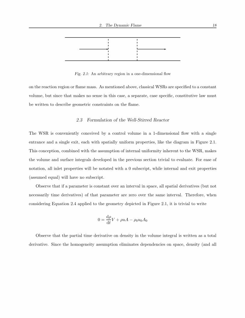
Fig. 2.1: An arbitrary region in a one-dimensional flow
on the reaction region or flame mass. As mentioned above, classical WSRs are specified to a constant
volume, but since that makes no sense in this case, a separate, case specific, constitutive law must
be written to describe geometric constraints on the flame.
2.3 Formulation of the Well-Stirred Reactor
The WSR is conveniently conceived by a control volume in a 1-dimensional flow with a single
entrance and a single exit, each with spatially uniform properties, like the diagram in Figure 2.1.
This conception, combined with the assumption of internal uniformity inherent to the WSR, makes
the volume and surface integrals developed in the previous section trivial to evaluate. For ease of
notation, all inlet properties will be notated with a 0 subscript, while internal and exit properties
(assumed equal) will have no subscript.
Observe that if a parameter is constant over an interval in space, all spatial derivatives (but not
necessarily time derivatives) of that parameter are zero over the same interval. Therefore, when
considering Equation 2.4 applied to the geometry depicted in Figure 2.1, it is trivial to write
0 =dρ
dtV + ρuA − ρ0u0A0
Observe that the partial time derivative on density in the volume integral is written as a total
derivative. Since the homogeneity assumption eliminates dependencies on space, density (and all
2. The Dynamic Flame 19
other parameters) is only a function of time. Defining the parameters
M ≡ ρV
m ≡ ρuA
m0 ≡ ρ0u0A0,
the continuity equation may be conveniently written as
ρ
ρ+
m − m0
M= 0. (2.10)
Note that because the boundaries of the reaction region are allowed to move in time, the entrance
and exit mass flows are not necessarily equal to the actual flow in and out of the control volume,
but are the local mass fluxes through a fixed location. For example, a control volume moving
with the flow has no entering or exiting flow, but would still have nonzero mass flow terms by this
conception. Applying the same process to the conservation of species, Equation 2.7 can be written
1
ρ
d
dt(ρYi) +
mYi − m0Yi,0
M=
ωi
ρ
Finally, by distributing the time derivative and substituting Equation 2.10,
Yi +m0
M(Yi − Yi,0) =
ωi
ρ.
It is at this point that it becomes convenient to combine certain terms for ease of notation because
of the frequency with which they will appear in later equations. The quantity ωi
ρis the reaction
rate of species i per unit mass. Since it is a term with physical significance that will appear quite
frequently let ζi ≡ ωi
ρ. Additionally, the quantity m0
Mwill prove to be of great significance to the
dynamic equations, so let σ ≡ m0
Mbe called the displacement rate. With these substitutions, the

2. The Dynamic Flame 20
species equation becomes much more elegant.
Yi + σ (Yi − Yi,0) = ζi. (2.11)
Observe that the displacement rate is in essence a measure of convection, related to the convective
particle mean residence time by σ = 1τres
. Once more, similar manipulations to Equation 2.9 yeild
1
ρ
d
dt(hρ) +
mh − m0h0
M= − Q
M+
1
ρ
dp
dt,
which can be simplified as above to yield
h + σ (h − h0) = − Q
M+
p
ρ. (2.12)
Equations 2.10, 2.11, and 2.12 are the fundamental governing equations for the dynamic WSR.
Just as with Equation 2.7, Equation 2.11 can be re-written for each of the species, so that if there are
n species, Equation 2.11 represents n independent equations. It is important to note that it would
be redundant to include Equation 2.10 as an independent law since it is now implicit in Equations
2.11 and 2.12, so there are n + 1 independent laws describing the system. If the reactor pressure is
considered an input that is determined by the acoustics surrounding the reactor (similar to the inlet
velocity), then n mass fractions and temperature remain to describe the reactor’s state. All that
remains for total closure of the system is the inclusion of a chemical kinetic model to determine
the reaction rates in Equation 2.11 and thermodynamic equations of state to allow calculation
of density, enthalpy, etc. in terms of temperature. As is discussed in the following section, the
application of very general thermodynamic principles, classical quantities such as the heat release
rate will appear naturally in the governing equations.
In order to apply Equations 2.11 and 2.12, it is necessary to select appropriate thermodynamic
equation of state. Though it is often inaccurate for some of the products common to combustion
(CO2) over the wide ranges of temperatures, the ideal gas law is favorably simple while arguably
sacrificing little accuracy in the model’s dynamic predictions. Therefore, for the purpose of this

2. The Dynamic Flame 21
work, however, density is evaluated by Equation 2.13.
ρ =p
RuT·(∑
i
Yi
MWi
)−1
(2.13)
It is also quite common to assume the species are perfect gases (Turns, Ghoniem, Lieuwen, Losh),
but this too can be quite inappropriate for combustion gases and the exclusion of this assumption
only slightly complicates the derivation. Though it will yield little in the way of novel results, the
improved acuracy and greater generality with little additional numerical cost warrants the analytical
effort. Consequent of the ideal gas assumption, enthalpy is only a function of temperature and the
species mass fractions. In the absence of the perfect gas assumption, enthalpy’s dependence on
temperature can be quite complicated, but its dependence on mass fraction can be given explicitly
based on the definition of an intensive property in a mixture
h (T, Yj) =∑
i
Yihi (T ) (2.14)
where hi is the enthalpy per unit mass of species i at temperature, T . Therefore, the time
derivative of enthalpy appearing in Equation 2.12 can be written as
h =∂h
∂TT +
∑
i
hiYi (2.15)
The partial derivative of enthalpy with respect to temperature is, by definition, specific heat at
constant pressure. This term is a function of both temperature and mass fraction. It is trivial to
show from Equation 2.14 that
cp =∑
i
Yicp,i, (2.16)
where the species’s specific heat is a function of temperature only. The relationship between
enthalpy and temperature is unique for each species and must be determined empirically. By
substituting Equations 2.14, 2.15, and 2.16 into Equation 2.12 where appropriate and performing
2. The Dynamic Flame 22
the necessary manipulation,
cpT + σ∑
i
Yi,0 (hi − hi,0) +∑
i
hi
(Yi + σ (Yi − Yi,0)
)= − Q
M+
p
ρ.
Observe that the left-hand side of Equation 2.11 appears exactly in the third term. Substitution
yields
cpT + σ∑
i
Yi,0 (hi − hi,0) = − Q
M+
p
ρ−∑
i
hiζi. (2.17)
The heat release rate term that naturally appears is an intensive property and must be integrated
over the entire mass in order to be total heat release rate.
H ≡ −∑
i
∫∫∫
Vr
hiζiρdV = −M∑
i
hiζi (2.18)
This is consistent with the more specialized equations in other works. Merely for the sake
of comparison with conventional simplifications, adding the perfect gas assumption implies that
specific heat is not a function of temperature and that a species’s enthalpy is related to temperature
linearly by the equation
hi = cp,iT + h0f,i
Substituting into Equation 2.17 and using Equation 2.16 to simplify, the result is
cp
cp,0T + σ (T − T0) = − Q
Mcp,0+
p
ρcp,0−∑
i
hf,i
cp,0ζi −
T
cp,0
∑
i
cp,iζi.
The last term in the right-hand side corrects for changes in specific heat as the contents of the
mixture change. However, a number of works with flame models have regarded cp equivalent for
all species at all temperatures. Though this assumption is by no means necessary to evaluate the
system, it does make the relevant physics much more conceptually accessible. If this is the case,
2. The Dynamic Flame 23
then the energy equation will finally take on the more familiar form,
T + σ (T − T0) = − Q
Mcp+
p
ρcp− 1
cp
∑
i
hf,iζi,
where the heat release rate, −∑i hf,iζi, is now a function of the enthalpy of formation of each
species only and not the total enthalpy.
2.4 Chemical Kinetics
The most accurate chemical kinetic models for the combustion of even simple fuels such as Methane
require hundreds of coupled, nonlinear rate equations, so it is necessary to abridge the chemical
kinetic model simply to aid in the analysis of the model results. Since any simplification in the
chemical kinetic model must inevitably sacrifice accuracy of some sort, it is important to select a
model that is appropriate to the application.
This particular work places no particular demand on the model’s ability to accurately predict
the concentrations of the various combustion products, nor flame temperature, nor even blow-off
limits, except to extent to which these parameters are important in determining the flame’s dynamic
heat release. Unfortunately it is very difficult to know a-priori what might influence the dynamic
response, but it will ultimately be shown that even crude approximations of the chemical kinetics
can offer great insight into the flame dynamics.
It is reasonable to assume that dynamics generated by the chemical kinetics are not impor-
tant in determining the cause of combustion instabilities since the qualitative dynamic behaviors
are contrary to common empirical knowledge surrounding the instabilities. At high combustion
temperatures (2000 K+), the reaction rates are high enough that rate-limiting time constants are
typically on the order of 10−5 or even 10−6 seconds, orders of magnitude faster than the 200 Hz or
lower instabilities observed in experimental combustors. At lower temperatures which are common
at the lean conditions where instabilities are most commonly noted, the characteristic time con-
stants can indeed drop to 10−3 seconds or even lower, but a reduction in the chemistry’s bandwidth
should arguably make the combustor tend to stability because of the reduction of gain local to
2. The Dynamic Flame 24
the instability frequency. Furthermore, this trend is contrary to the empirical observations that
well-mixed flames tend to have broader bandwidths at lower equivalence ratios.
In the absence of the empirical observations of flame bandwidth this assumption is admittedly
suspect. In fact, additional dynamics in the vicinity of the acoustic poles can have the effect of
adding potentially destabilizing phase despite the reduction in gain. It will be shown, however, that
transport dynamics may be sufficient to describe the predominant dynamics in well-mixed flames,
even at lean conditions. Therefore, the choice in chemical kinetic model need only be sensitive to
accurate static predictions.
Global chemical kinetic models are empirical by nature and presume to model combustion with
a single chemical equation that ignores intermediate species. These models have been used widely to
make static predictions for flame temperature and blow-off limits. Despite the gross nonlinearities
inherent to such a model, its relative simplicity makes it a natural choice for this work. A discussion
on the details of Arrhenius kinetics is beyond the purview of this document, particularly since global
single-step mechanisms are related by form alone to the Arrhenius kinetics.
A single-step, global chemical equation takes the form
ν ′
1X1 + ν ′
2X2 + . . . + ν ′
nXn → ν ′′
1X1 + ν ′′
2X2 + . . . + ν ′′
nXn (2.19)
where ν ′
i is the coefficient of species Xi on the reactants side and ν ′′
i is the coefficient of species Xi
on the products side of the equation. Note that X is not used here to denote the mole fraction of
the species, rather as a blanked way of expressing multiple species. Observe also, that the reaction
is irreversible and assumes that all species appear in both the reactants and products in order to
maintain generality. In fact, the actual hydrocarbon combustion reaction appears
CxHyOz + aO2 → bCO2 + cH2O.
2. The Dynamic Flame 25
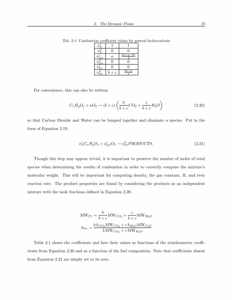
Tab. 2.1: Combustion coefficient values for general hydrocarbons
ν ′
F 1 1
ν ′′
F 0 0
ν ′
Ox a 4x+y−2x4
ν ′′
Ox 0 0
ν ′
Pr 0 0
ν ′′
Pr b + c 2x+y2
For convenience, this can also be written
CxHyOz + aO2 → (b + c)
(b
b + cCO2 +
c
b + cH2O
)(2.20)
so that Carbon Dioxide and Water can be lumped together and eliminate a species. Put in the
form of Equation 2.19,
ν ′
F CxHyOz + ν ′
OxO2 → ν ′′
PrPRODUCTS. (2.21)
Though this step may appear trivial, it is important to preserve the number of moles of total
species when determining the results of combustion in order to correctly compute the mixture’s
molecular weight. This will be important for computing density, the gas constant, R, and even
reaction rate. The product properties are found by considering the products as an independent
mixture with the mole fractions defined in Equation 2.20.
MWPr =b
b + cMWCO2
+c
b + cMWH2O
hPr =b hCO2
MWCO2+ c hH2OMWC2O
bMWCO2+ cMWH2O
Table 2.1 shows the coefficients and lists their values as functions of the stoichiometric coeffi-
cients from Equation 2.20 and as a function of the fuel composition. Note that coefficients absent
from Equation 2.21 are simply set to be zero.

2. The Dynamic Flame 26
Thus far, three species (fuel, oxidizer, and products) are defined in the context of the classical
combustion reaction. Absent, however, is any species that does not participate in the reaction.
Though trivial to the chemical reaction since such species are neither formed nor depleted by the
reaction, these species dilute the mixture and absorb heat, slowing the reaction rate. For this
reason, such species are called diluent.
Reaction Rate
The reaction rate can be described as the number of times a given reaction occurs per unit volume
per unit time. The variable, q, also called the “reaction progress”, is often used to represent the
reaction rate in single-step global chemical systems. It is common to express q in moles per unit time
per unit volume, since the number would otherwise be quite large. This is a useful nomenclature
since q takes the meaning of reaction speed in general and is nonspecific to a particular species. q is
typically expressed as an explicit function of the local temperature and species concentrations even
though intuition seems to indicate that the reaction rate should also depend on pressure. It will be
shown that such a dependence does actually exist, but it is purely implicit. The Arrhenius form
of the reaction rate equation in particular presumes an exponential dependence on the inverse of
temperature and power dependencies on the concentrations of the various reactants, thus allowing
q to be expressed
q = A exp
(− Ea
RuT
)∏
i
Cimi
In this expression, A, Ea, and mi are purely empirical parameters, and Ci is the concentration
of the ith species. The activation energy, Ea, is of particular interest since its ratio with the ideal
gas constant represents a temperature above which the reaction is quite fast (called the activation
temperature).
This equation can be simplified by adding the condition that forward reactions are independent
of the product concentrations (that only the reactants influence the reaction rate), so that the
2. The Dynamic Flame 27
reaction rate for Equation 2.21 is
q = A exp
(− Ea
RuT
)CF
mCOxn. (2.22)
For each reaction, the number of moles of a particular species that are either depleted or
formed can be determined by the specie’s stoichiometric coefficients in the reaction equation. Since
this refers to the depletion or formation of species per unit volume, the result is a change in
concentration. Therefore, changes in individual species concentrations are governed by
dCi
dt=(ν ′′
i − ν ′
i
)A exp
(− Ea
RuT
)CF
mCOxn. (2.23)
Since concentrations and molar formation rates are difficult to apply to fluid equations, it is
helpful to convert the molar units into material units (mass). It is trivial to show from their
definitions that mass fraction is related to concentration by
Ci = Yiρ
MWi
Similarly, the formation of species in material units can be related to concentration by the
expression
ζi =MWi
ρ
dCi
dt
Therefore,
ζi = MWi
(ν ′′
i − ν ′
i
)A exp
(− Ea
RuT
)(YF
MWF
)m( YOx
MWOx
)n
ρm+n−1. (2.24)
Note from Equation 2.2.3 that the formation or depletion of each species is related to the other
2. The Dynamic Flame 28
species by a simple proportion that does not change in time, since
ζi
ζj=
MWi(ν′′
i − ν ′
i)
MWj(ν ′′
j − ν ′
j)(2.25)
Therefore, it is trivial in a system modeled with a single-step global mechanism to write the
heat release in Equation 2.18 in terms of the reaction rate for a specific species. This allows the
customary formulation of heat release with respect to the fuel reaction rate
H ≡ −Mζi∆hi (2.26)
for any species, i, where ∆hi is the temperature-dependent local heating value with respect to the
same species. The local heating value is the heat released per unit mass formed of the respective
species, and is most intuitively expressed in terms of the fuel. The local heating value with respect
to an arbitrary species can be derived from Equations 2.18 and 2.25, resulting in
∆hi ≡∑
j hjMWj(ν′′
j − ν ′
j)
MWi(ν ′′
i − ν ′
i). (2.27)
With these simplified kinetics, not only are the heat release rate and reaction rate much simpler
quantities to compute, but the limited number of species present in the model also permits generous
simplification of the general equations of motion. There are a total of four species included in the
model: fuel, oxidizer, product, and diluent. Including the energy equation, this would tend to
imply that five equations of motion are necessary to define the flame. By definition, however,
1 = Yf + Yox + Ydil + Ypr,
at all locations in space. So, one of the four species can always (dynamically or statically) be
written in terms of the other three. Secondly, note that the conservation of species for diluent is
Ydil + σ(Ydil − Ydil,0) = 0.

2. The Dynamic Flame 29
The diluent reaction rate is automatically zero since it does not participate in the single-step reac-
tion mechanism. Its only effect, therefore, is implicit through the reduction of flame temperature.
Furthermore, the only means for Ydil to vary dynamically is through unsteady convection. While
mixing perturbations will, indeed provide exactly that, it can be shown with a far more detailed
analysis than is productive in the context of this discussion that this effect is negligible and that
the diluent mass fraction can simply be considered a constant parameter, Ydil.
Therefore, it is possible to eliminate two of these five governing equations. Since fuel and
oxidizer appear explicitly in the reaction rate, it is most convenient to eliminate the products as
well as diluent. Therefore, for the purposes of this work,
Ydil = const. (2.28)
Ypr = 1 − Yf − Yox − Ydil, (2.29)
leaving a total of three governing equations which will be analyzed in detail in the proceeding
sections.
2.5 Analysis by Perturbations
Fundamental to linear stability analysis of any system is the assertion that whatever disturbances
are responsible for perturbing the system from equilibrium are small enough to elicit an initial
response consistent with that of a linear system. When this is the case, whether the response is
thereafter allowed to grow sufficiently as to exhibit nonlinear characteristics is determined exclu-
sively while the system is operating in the linear regime. Cases with larger excitations or larger
initial conditions that place the system in a nonlinear regime must inevitably be exceptions to this
type of analysis and can potentially exhibit very different behaviors.
Nayfeh has very elegantly dealt with many forms of this type of analysis in his book[15]. Therein,
it is observed that if any dynamic input to a nonlinear system (such as a flame) is scaled by a small,
dimensionless parameter, ε, then the response in the nonlinear system can be expanded in a Taylor
series on ε such that each term is exclusively a function in time and higher order terms are of

2. The Dynamic Flame 30
declining importance to the computation of the response. Consider, for example, a nonlinear
system,
x = f(x,u)
If the input, u is decomposed into steady and dynamic components as described, then
u = u + εu(t)
and
x = x(t; ε) = x + εx(t) + ε2˜x(t) + . . .
As a result
ε ˙x(t) + ε2 ˙x(t) + . . . = f(x,u) + ε
(∂f(x,u)
∂xx(t) +
∂f(x,u)
∂uu(t)
)+ ε2
(. . .
)+ . . .
Naturally, this expansion is continued infinitely, but since ε is presumed to be small, progressively
higher terms have a diminishing impact on the solution, encouraging their omission. In fact, this
is precisely what must be done in order to ensure the system’s linearity since non-proportional
(quadratic and higher-order) dependencies on the amplitude of the excitation, ε, characterizes a
strictly non-linear response.
Therefore, isolating the remaining two terms and remembering that equal polynomials have
equal coefficients,
0 = f(x,u) (2.30a)
˙x =∂f(x,u)
∂xx(t) +
∂f(x,u)
∂uu(t). (2.30b)
These equations represent linear, time invariant, equations. The first is an algebraic constraint
governing the steady-state of the system. Given the steady component to an input, u, Equation
2. The Dynamic Flame 31
2.30a allows computation the steady component of the response, x. Once computed, these are used
to evaluate Equation 2.30b using traditional state-space methods.
As established in Section 1.3, the inputs of interest for this work are mass flow and equivalence
ratio. The inputs to the flame model should therefore be expressed as
m(t) = m + ε ˜m(t) (2.31a)
Φ(t) = Φ + ε Φ(t), (2.31b)
where m and Φ represent the steady mass flow and equivalence ratio respectively, ˜m(t) and Φ(t)
are respective unsteady mass flow and equivalence ratio functions. Careful analysis of the gov-
erning equations established in Section 2.3 reveals all other internal flame parameters that are not
parametrically defined external to the model (such as density, reaction rate, total molecular weight,
etc. . . ) can be written explicitly in terms of internal flame temperature and the mass fractions.
The flame’s state can therefore be written as
T (t; ε) = T + ε T (t) + ε2 ˜T (t) + . . . (2.32a)
Yi(t; ε) = Y i + ε Yi(t) + ε2 ˜Y i(t) + . . . (2.32b)
For simplicity, this investigation is conducted under the additional assumption that the reactor
is adiabatic. Naturally, that is utter nonsense since radiation and convection both are rampant, but
the assertion is that these phenomena do not significantly affect the dynamic characteristics. Given
the generous simplification it affords and that similar abstractions are abound in the literature[11,
19, 18] apparently without consequence, it is well worth the departure from physical truth.
Taking the simplifications in heat release rate from Equation 2.26, the new adiabatic assumption,
the assumption discussed in Section 1.3 that pressure perturbations have a negligible effect, and
2. The Dynamic Flame 32
the governing equations developed in Section 2.3 the simplified governing equations are
cpT + σ∑
i
Yi,0 (hi − hi,0) = −∆hfζf (2.33)
Yi + σ (Yi − Yi,0) = ζi, (2.34)
where as above, the reaction rate, ζi, and heat release per mass of species consumed, ∆hi, are
respectively given as
ζi = MWi
(ν ′′
i − ν ′
i
)A exp
(− Ea
RuT
)(YF
MWF
)m( YOx
MWOx
)n
ρm+n−1
and
∆hi ≡∑
j hjMWj(ν′′
j − ν ′
j)
MWi(ν ′′
i − ν ′
i).
The excitation parameters, mass flow and equivalence ratio, do not appear explicitly in any
of these expressions, rather they appear as implicit parametric excitations through σ and Yi,0
respectively. Firstly, recall that
σ ≡ m0
M. (2.35)
The flame mass, M , is still an ambiguous quantity with an undetermined dependence on the flame
state and the inputs. To avoid loss of generality at this point in discussing the system, therefore,
it becomes necessary to simply write M = M(T, Yi,m0,Φ). Clearly, mass flow perturbations will
influence σ directly, but what role M plays can only be determined when it is similarly expanded
out in terms of the state variables and input. To that end, there are several candidate methods for
constraining the flame which will be discussed in Section 2.8.
Equivalence ratio perturbations, on the other hand, simply manifest themselves in inlet mass
fraction perturbations, Yi,0. Presuming that the air entering the combustor consists of a constant

2. The Dynamic Flame 33
mixture of oxygen and diluent, Ydil,0 = αYox,0. In the absence of combustion product upstream of
the flame,
1 = Yf,0 + Yox,0 + Ydil,0 = Yf,0 + (1 + α)Yox,0. (2.36)
By definition,
Φ =Yf,0
Yox,0
(Yf
Yox
∣∣∣∣Stoich
)−1
=Yf,0
Yox,0β−1
if β ≡ Yf
Yox
∣∣∣Stoich
, which is a constant for a given fuel. Combining these two equations and solving
for Yf,0,
Yf,0 =βΦ
(α + 1) + βΦ(2.37a)
Simple additional manipulation can easily show,
Yox,0 =1
(α + 1) + βΦ(2.37b)
Ydil,0 =α
(α + 1) + βΦ(2.37c)
From this point, it is convenient to divide the discussion into two parts: the solution of the
steady system represented by Equation 2.30a, and the frequency response of the dynamic system
represented by Equation 2.30b.
2.6 The Physical Dynamic Flame
In order to assess the success of the model in describing the flame, it is necessary to have a “truth”
for comparison. There have been a few dynamic flame experiments of note in the literature, but
none that deal directly with the needs of this particular work. Most notably, the data collected
by Lohrmann and Buchner[12] included the dynamic response of the flame’s heat release rate to
mass flow fluctuations induced by an upstream speaker for various mean mass flows and upstream

2. The Dynamic Flame 34
temperatures, but neglected to study the flame’s response to equivalence ratio variations. Both to
reexamine the prevailing notions surrounding turbulent flame dynamics and to develop novel results
specifically relevant to the flame component model, the Virginia Active Combustion Control Group
(VACCG) initiated a parallel effort to characterize a physical flame’s dynamics.
The Findings of Lohrmann and Buchner
Lohrmann and Buchner excited a swirl-stabilized premixed flame with a speaker placed upstream
and measured the flame heat release rate transfer function with respect to upstream velocity per-
turbations for a variety of inlet temperatures. Though their work focuses on effects due to the
single inlet parameter that this document has elected to neglect, the results are directly applicable
the discussion at hand.
The most relevant of their observations was that as upstream temperature increases, so does
the bandwidth of the flame. Since they measured both the magnitude and phase of the flame’s
response (both of which are absolutely necessary for determining systemic stability) they were also
able to note declining delay in the flame transfer function with increasing upstream temperature.
Finally, they defined the Strouhal number for their flame by
Str ≡ fx
u, (2.38)
where f is the frequency of interest, x is a length scale of the flame, and u is a velocity scale of the
flame, and noted that when the frequency response was plotted against the Strouhal number, the
scaled bandwidth and delay became nearly identical for all cases of inlet temperature. The implica-
tion is that regardless of the impact the upstream temperature may have had on chemical kinetics,
the flame’s dynamics scale perfectly with mechanically derived time scales. In this particular case,
the time scale in question is the mean particle residence time, roughly estimated by τres = 2xu
for
Lohrmann and Buchner’s case.
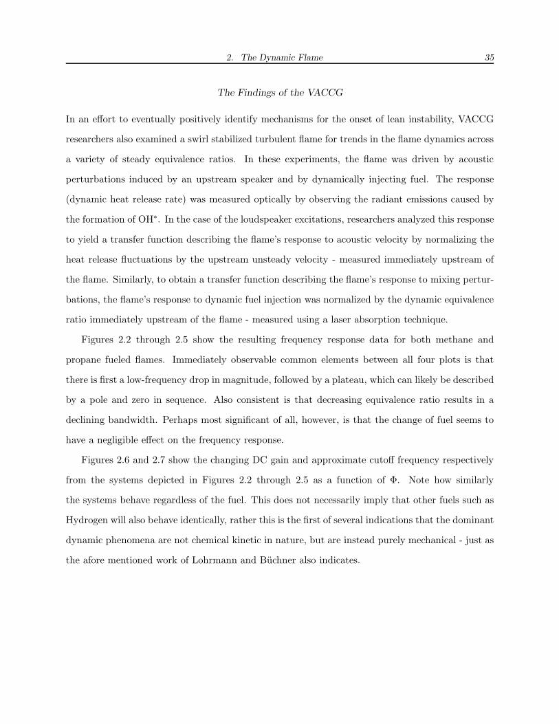
2. The Dynamic Flame 35
The Findings of the VACCG
In an effort to eventually positively identify mechanisms for the onset of lean instability, VACCG
researchers also examined a swirl stabilized turbulent flame for trends in the flame dynamics across
a variety of steady equivalence ratios. In these experiments, the flame was driven by acoustic
perturbations induced by an upstream speaker and by dynamically injecting fuel. The response
(dynamic heat release rate) was measured optically by observing the radiant emissions caused by
the formation of OH∗. In the case of the loudspeaker excitations, researchers analyzed this response
to yield a transfer function describing the flame’s response to acoustic velocity by normalizing the
heat release fluctuations by the upstream unsteady velocity - measured immediately upstream of
the flame. Similarly, to obtain a transfer function describing the flame’s response to mixing pertur-
bations, the flame’s response to dynamic fuel injection was normalized by the dynamic equivalence
ratio immediately upstream of the flame - measured using a laser absorption technique.
Figures 2.2 through 2.5 show the resulting frequency response data for both methane and
propane fueled flames. Immediately observable common elements between all four plots is that
there is first a low-frequency drop in magnitude, followed by a plateau, which can likely be described
by a pole and zero in sequence. Also consistent is that decreasing equivalence ratio results in a
declining bandwidth. Perhaps most significant of all, however, is that the change of fuel seems to
have a negligible effect on the frequency response.
Figures 2.6 and 2.7 show the changing DC gain and approximate cutoff frequency respectively
from the systems depicted in Figures 2.2 through 2.5 as a function of Φ. Note how similarly
the systems behave regardless of the fuel. This does not necessarily imply that other fuels such as
Hydrogen will also behave identically, rather this is the first of several indications that the dominant
dynamic phenomena are not chemical kinetic in nature, but are instead purely mechanical - just as
the afore mentioned work of Lohrmann and Buchner also indicates.

2. The Dynamic Flame 36
Fig. 2.2: Methane heat release rate response to velocity perturbations. (Ranalli)
Fig. 2.3: Methane heat release rate response to equivalence ratio perturbations. (Ranalli)
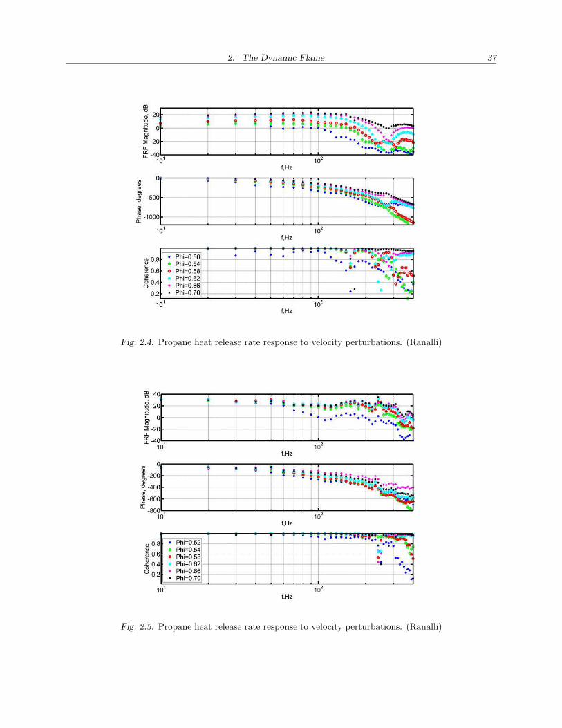
2. The Dynamic Flame 37
Fig. 2.4: Propane heat release rate response to velocity perturbations. (Ranalli)
Fig. 2.5: Propane heat release rate response to velocity perturbations. (Ranalli)

2. The Dynamic Flame 38
Fig. 2.6: Dynamic data summary: DC Gains. (Ranalli)
Fig. 2.7: Dynamic data summary: Bandwidths. (Ranalli)

2. The Dynamic Flame 39
2.7 Steady Solution of the Well-Stirred Reactor
As indicated by Equation 2.30a, the steady solution of a dynamic system is that which satisfies the
equations of motion subject to purely steady excitations. Therefore, the equations governing the
steady flame are
σ∑
i
Y i,0
[hi(T ) − hi(T0)
]= −∆hf (T )ζf (T , Y f , Y ox) (2.39a)
σ(Y f − Y f,0) = ζf (T , Y f , Y ox) (2.39b)
σ(Y ox − Y ox,0 = ζox(T , Y f , Y ox), (2.39c)
with steady external parameters, T0, Y f,0, Y ox,0, σ given. Note that T0 has no overbar to identify
it as a steady parameter. This is because within the context of this model, upstream temperature
is not allowed to vary dynamically and is therefore automatically steady.
Solution Paths for the Steady Reactor
What follows may boarder on the tedious in its detail devoted to the iterative solution of these
algebraic equations. If it does, it is justified only because so many other works have either failed
to describe their method in sufficient detail to allow accurate reproduction, or because yet more
works have presumed to take on added, unnecessary assumptions, resulting in a distinct lack of
attention given to accurate computation of steady reactor conditions in the literature. To simplify
the notation in this section, let the overbars notating these as steady conditions be taken as wrote.
Quite naturally once beginning the discussion of the flame dynamics, this notation will resume.
First, note from Equation 2.39b that
∆Yf ≡ Yf − Yf,0 =ζf
σ, (2.40)
and that a similar relation also exists for the oxidizer mass fraction. From Equation 2.25, it follows
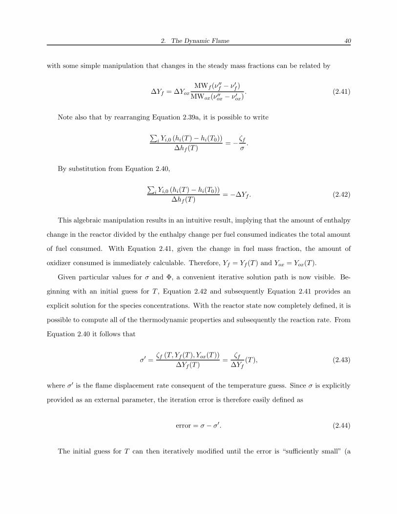
2. The Dynamic Flame 40
with some simple manipulation that changes in the steady mass fractions can be related by
∆Yf = ∆Yox
MWf (ν ′′
f − ν ′
f )
MWox(ν ′′
ox − ν ′
ox). (2.41)
Note also that by rearranging Equation 2.39a, it is possible to write
∑i Yi,0 (hi(T ) − hi(T0))
∆hf (T )= −ζf
σ.
By substitution from Equation 2.40,
∑i Yi,0 (hi(T ) − hi(T0))
∆hf (T )= −∆Yf . (2.42)
This algebraic manipulation results in an intuitive result, implying that the amount of enthalpy
change in the reactor divided by the enthalpy change per fuel consumed indicates the total amount
of fuel consumed. With Equation 2.41, given the change in fuel mass fraction, the amount of
oxidizer consumed is immediately calculable. Therefore, Yf = Yf (T ) and Yox = Yox(T ).
Given particular values for σ and Φ, a convenient iterative solution path is now visible. Be-
ginning with an initial guess for T , Equation 2.42 and subsequently Equation 2.41 provides an
explicit solution for the species concentrations. With the reactor state now completely defined, it is
possible to compute all of the thermodynamic properties and subsequently the reaction rate. From
Equation 2.40 it follows that
σ′ =ζf (T, Yf (T ), Yox(T ))
∆Yf (T )=
ζf
∆Yf(T ), (2.43)
where σ′ is the flame displacement rate consequent of the temperature guess. Since σ is explicitly
provided as an external parameter, the iteration error is therefore easily defined as
error = σ − σ′. (2.44)
The initial guess for T can then iteratively modified until the error is “sufficiently small” (a
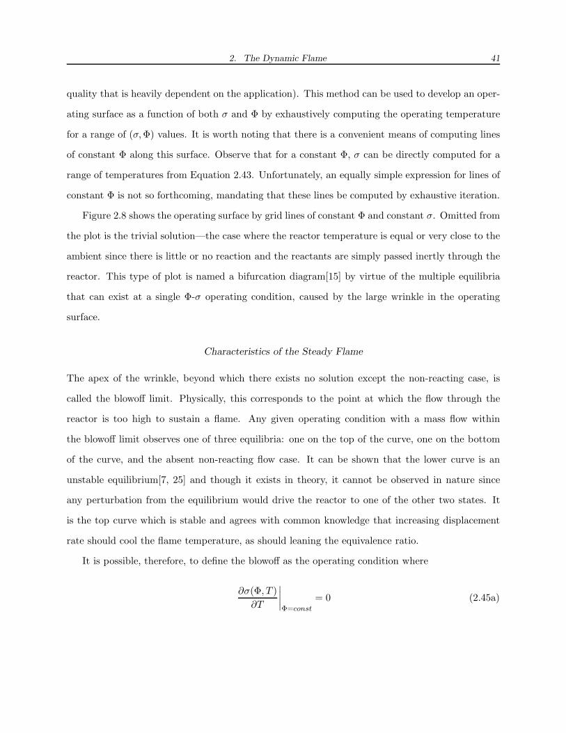
2. The Dynamic Flame 41
quality that is heavily dependent on the application). This method can be used to develop an oper-
ating surface as a function of both σ and Φ by exhaustively computing the operating temperature
for a range of (σ,Φ) values. It is worth noting that there is a convenient means of computing lines
of constant Φ along this surface. Observe that for a constant Φ, σ can be directly computed for a
range of temperatures from Equation 2.43. Unfortunately, an equally simple expression for lines of
constant Φ is not so forthcoming, mandating that these lines be computed by exhaustive iteration.
Figure 2.8 shows the operating surface by grid lines of constant Φ and constant σ. Omitted from
the plot is the trivial solution—the case where the reactor temperature is equal or very close to the
ambient since there is little or no reaction and the reactants are simply passed inertly through the
reactor. This type of plot is named a bifurcation diagram[15] by virtue of the multiple equilibria
that can exist at a single Φ-σ operating condition, caused by the large wrinkle in the operating
surface.
Characteristics of the Steady Flame
The apex of the wrinkle, beyond which there exists no solution except the non-reacting case, is
called the blowoff limit. Physically, this corresponds to the point at which the flow through the
reactor is too high to sustain a flame. Any given operating condition with a mass flow within
the blowoff limit observes one of three equilibria: one on the top of the curve, one on the bottom
of the curve, and the absent non-reacting flow case. It can be shown that the lower curve is an
unstable equilibrium[7, 25] and though it exists in theory, it cannot be observed in nature since
any perturbation from the equilibrium would drive the reactor to one of the other two states. It
is the top curve which is stable and agrees with common knowledge that increasing displacement
rate should cool the flame temperature, as should leaning the equivalence ratio.
It is possible, therefore, to define the blowoff as the operating condition where
∂σ(Φ, T )
∂T
∣∣∣∣Φ=const
= 0 (2.45a)

2. The Dynamic Flame 42
0.50.6
0.70.8
0.91
0
5000
10000
15000
400
600
800
1000
1200
1400
1600
1800
2000
2200
2400
σ (1/s)Φ
T, K
Fig. 2.8: WSR temperature bifurcation diagram. Equilibria temperatures are plotted against Φ and σ. Linesof constant Φ are in black and lines of constant σ are in blue.
at a given Φ and
∂Φ(σ, T )
∂T
∣∣∣∣σ=const
= 0 (2.45b)
at a given σ. Expanding Equation 2.45a using Equation 2.43, it follows that
1
ζf
∂ζf
∂T
∣∣∣∣Φ=const
=1
∆Yf
∂∆Yf
∂T
∣∣∣∣Φ=const
. (2.46)
It is a simple matter to then solve for T to satisfy this condition and back calculate all the other
properties, including σ. The blowoff temperature is the lowest temperature at which the WSR can
predict a stable flame for a given equivalence ratio.
The highest temperature the WSR can predict corresponds to the case when σ = 0, representing
the complete combustion of a stagnant plug of premixed fuel and air with no heat loss. From any
of the three steady equations of motion, it follows that a zero value for σ implies that ζ is also
zero. Reaction rate only goes to zero when either the fuel or oxidizer have been completely depleted
(excluding the possibility of reactor temperature being 0K), ergo the combustion is complete. In a
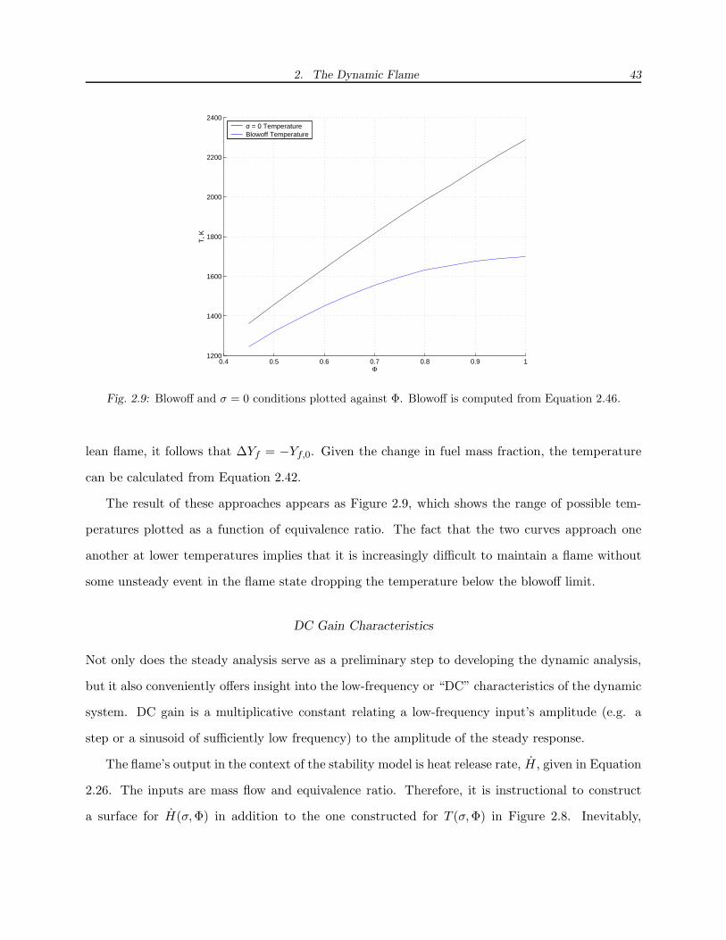
2. The Dynamic Flame 43
0.4 0.5 0.6 0.7 0.8 0.9 11200
1400
1600
1800
2000
2200
2400
Φ
T, K
σ = 0 TemperatureBlowoff Temperature
Fig. 2.9: Blowoff and σ = 0 conditions plotted against Φ. Blowoff is computed from Equation 2.46.
lean flame, it follows that ∆Yf = −Yf,0. Given the change in fuel mass fraction, the temperature
can be calculated from Equation 2.42.
The result of these approaches appears as Figure 2.9, which shows the range of possible tem-
peratures plotted as a function of equivalence ratio. The fact that the two curves approach one
another at lower temperatures implies that it is increasingly difficult to maintain a flame without
some unsteady event in the flame state dropping the temperature below the blowoff limit.
DC Gain Characteristics
Not only does the steady analysis serve as a preliminary step to developing the dynamic analysis,
but it also conveniently offers insight into the low-frequency or “DC” characteristics of the dynamic
system. DC gain is a multiplicative constant relating a low-frequency input’s amplitude (e.g. a
step or a sinusoid of sufficiently low frequency) to the amplitude of the steady response.
The flame’s output in the context of the stability model is heat release rate, H, given in Equation
2.26. The inputs are mass flow and equivalence ratio. Therefore, it is instructional to construct
a surface for H(σ,Φ) in addition to the one constructed for T (σ,Φ) in Figure 2.8. Inevitably,

2. The Dynamic Flame 44
0.5
0.6
0.7
0.8
0.9
1
0
5000
10000
15000
0
0.5
1
1.5
2
2.5
3
3.5
4
x 106
σ (1/s)
Φ
Hea
t Rel
ease
Rat
e (W
)
Fig. 2.10: WSR heat release rate bifurcation diagram. Equilibria heat release rates are plotted against Φand σ. Lines of constant Φ are in black and lines of constant σ are in blue.
this returns to the troubling question of how to define the flame’s size since M appears explicitly
both in the definition of heat release rate. Some assumption must be made if this analysis is to
proceed. Traditionally, the volume of the reactor is held constant[25, 7, 11, 18], but this arbitrary
method is neither convenient nor physically motivated. On the other hand, assuming M to be
constant is equally arbitrary and also lacks physical motivation but has the added convenience of
greatly simplifying the derivation to come. Very similar results can also be achieved through other
assumptions on M [18], but this is the most conducive to discussion.
Granted this generous abstraction, the surface shown in Figure 2.10 can be generated simply by
calculating the heat release rate from the reactor states already computed for Figure 2.8. Similar
to the temperature bifurcation diagram, it can be shown that the upper surface represents stable
operating conditions while the lower one represents unstable ones.
Note that if the curve shown in Figure 2.10 is the steady output of the flame as a function of
the two steady inputs, then the DC gain with respect to either of the inputs at any given operating
condition is the local slope of that curve along the axis belonging to the input in question. Then

2. The Dynamic Flame 45
the DC gains of the system with respect to σ and Φ respectively are
Km =∂H(σ,Φ)
∂σ
∂σ
∂m
∣∣∣∣∣Φ=const
(2.47a)
KΦ =∂H(σ,Φ)
∂Φ
∣∣∣∣∣σ=const
(2.47b)
Simply from the definition of heat release rate in Equation 2.18 and σ in Equation 2.35,
Km = − ∂ (∆hf ζf )
∂σ
∣∣∣∣Φ=const
KΦ = −M∂ (∆hf ζf )
∂Φ
∣∣∣∣σ=const
.
Observe that when the identity for σ is substituted into Equation 2.47a and if M is presumed a
constant parameter, the M in the heat release rate definition is canceled, leaving a very convenient
form. The validity assuming constant M with respect to σ and Φ will be discussed in detail later,
but for the purposes of calculating DC gains, it introduces negligible error.
It provides great insight both into why these gains diverge at blowoff and into how to calculate
them to recall that temperature as an intermediate variable in the calculation of heat release rate.
Note that the entire numerator can be expressed explicitly in terms of temperature when isolated
to a line of constant Φ or constant σ, which ultimately allows the derivatives to be expanded to
yield
Km = −[d (∆hf ζf )
dT
∂T
∂σ
]
Φ=const
(2.48a)
KΦ = −M
[d (∆hfζf )
dT
∂T
∂Φ
]
σ=const
. (2.48b)
However, this evokes exactly the terms which were used in the definition of blowoff in Equations
2. The Dynamic Flame 46
2.45b and 2.45a. In the limit as the operating conditions approach blowoff,
∂T
∂σ
∣∣∣∣Φ=const
=
(∂σ
∂T
∣∣∣∣Φ=const
)−1
blowoff→ −∞
∂T
∂Φ
∣∣∣∣σ=const
=
(∂Φ
∂T
∣∣∣∣σ=const
)−1
blowoff→ ∞.
It is therefore conclusive that unless the definition of blowoff is allowed to change, heat release rate
DC gains will always diverge at operating conditions close to blowoff. There can be little doubt
that this is candidate explanation for instabilities that occur with ultra-lean flames.
The plots in Figure 2.12 show the DC gains plotted against the two steady operating parame-
ters. These curves are calculated from Equations 2.48a and 2.48b using the relationships given in
Equations 2.40 through 2.43.
Ghoniem et al[18] found almost identical results for subplot (a) of Figure 2.12 a change in sign
(as well as diverging to −∞), causes a 180◦ shift in phase, which has a great potential to cause
instability. It is also to be noted, however, that the response to equivalence ratio perturbations
(which was absent from the particular work referenced) also diverges and begins to do so much
further from blowoff than does the response to mass flow perturbations. This result requires very
little imagination to infer how ultra-lean instabilities can occur.
2.8 Bandwidth and Frequency Response
If the steady component of the flame’s response is contained in the first term of the expansion
discussed in Section 2.5, then those remaining represent the dynamic response. As discussed in
Section 2.5, the linear dynamic response may be taken to be the first term to the Taylor Series
expansion on ε. Just as was done in Section 2.7 to obtain the steady response, the dynamic response
is obtained by equating like coefficients of ε as in Equation 2.30b. Using Equations 2.33 and 2.34
as the equations of motion, this yields
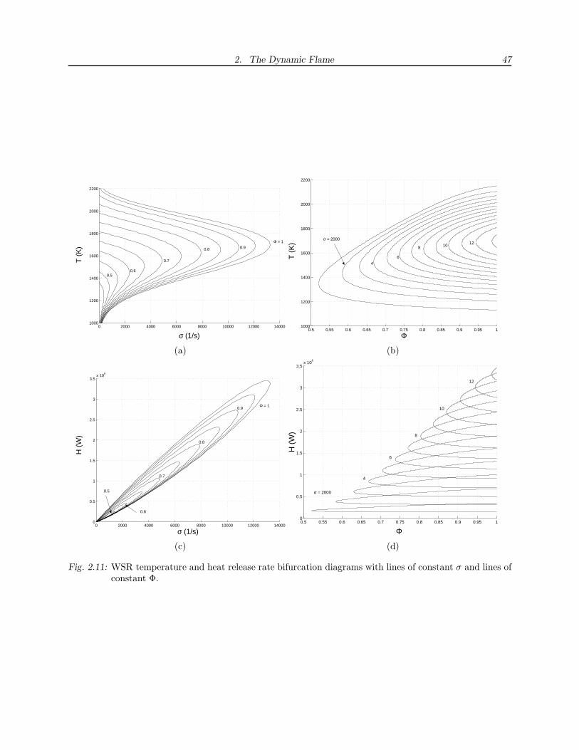
2. The Dynamic Flame 47
0 2000 4000 6000 8000 10000 12000 140001000
1200
1400
1600
1800
2000
2200
T (
K)
σ (1/s)
0.50.6
0.7
0.8 0.9Φ = 1
0.5 0.55 0.6 0.65 0.7 0.75 0.8 0.85 0.9 0.95 11000
1200
1400
1600
1800
2000
2200
T (
K)
Φ
σ = 2000
4
6
8 10 12
(a) (b)
0 2000 4000 6000 8000 10000 12000 140000
0.5
1
1.5
2
2.5
3
3.5x 10
6
H (
W)
σ (1/s)
0.5
0.6
0.7
0.8
0.9Φ = 1
0.5 0.55 0.6 0.65 0.7 0.75 0.8 0.85 0.9 0.95 10
0.5
1
1.5
2
2.5
3
3.5x 10
6
H (
W)
Φ
σ = 2000
4
6
8
10
12
(c) (d)
Fig. 2.11: WSR temperature and heat release rate bifurcation diagrams with lines of constant σ and lines ofconstant Φ.

2. The Dynamic Flame 48
0 0.1 0.2 0.3 0.4 0.5 0.6 0.7 0.8 0.9 10.5
1
1.5
2
2.5x 10
6
σ / σbo
Km
(W
−s/
kg)
Φ = 0.55
0.65
0.75
0 0.1 0.2 0.3 0.4 0.5 0.6 0.7 0.8 0.9 10.5
1
1.5
2
2.5x 10
6
(Φ − Φbo
) / (1 − Φbo
)
Km
(W
−s/
kg)
2
4
σ = 6
(a) (b)
0 0.1 0.2 0.3 0.4 0.5 0.6 0.7 0.8 0.9 10
0.5
1
1.5
2
2.5
3
3.5
4
4.5
5x 10
6
σ / σbo
KΦ
(W
)
0.55
0.65
Φ = 0.75
0 0.1 0.2 0.3 0.4 0.5 0.6 0.7 0.8 0.9 10
0.5
1
1.5
2
2.5
3
3.5
4
4.5
5x 10
6
(Φ − Φbo
) / (1 − Φbo
)
KΦ
(W
)
σ = 2000
4
6
(c) (d)
Fig. 2.12: Flame DC gains plotted against the non-dimensionalized steady system parameters. σ has simplybeen scaled so that 1 corresponds to blowoff, while Φ has been scaled and shifted so that 0 is leanblowoff and 1 is an equivalence ratio of 1.

2. The Dynamic Flame 49
cp˙T + σ
∑
i
Y i,0hi = σ∑
i
Y i,0
(hi0 − hi
)+ σ
∑
i
Yi,0
(hi0 − hi
)− ∆hf ζf − ∆hf ζf (2.49a)
˙Y i + σ
(Yi − Yi,0
)= σ
(Y i,0 − Y i
)+ ζi. (2.49b)
Many of the unsteady parameters that appear in Equations 2.49a and 2.49b are already explicitly
in terms of either inputs (Yi,0) or state variables (Yi and T ). In order to consider the remaining
parameters (ζi, σ, or ∆hf ), they must be expressed in terms of their sensitivities to the state
variables and inputs. Calling Yi,0 an input is not an attempt to retract the earlier assertion that
the inputs will be ˜m0 and Φ, but an acknowledgment that it will prove simpler to assert the
identities in Equations 2.37a, 2.37b, and 2.37c later rather than sooner.
Recall that
hi = hi(T )
∆hf = ∆hf (T )
ζi = ζi(T, Yf , Yox)
σ =m0
M
M = M(T, Yf , Yox, m0, Yf,0, Yox,0).
Equations 2.55a, 2.55b, and 2.55c show the first expansion for all of these quantities. Note that
in order to evaluate ζi’s dependence on any of the state variables, ζ must be expanded to include not
only the explicit dependencies that appear in Equation 2.24 but also the implicit dependencies that
are introduced through density and molecular weight. This total expansion is tedious and would
detract from the discussion more than it would add were it to be included. As it is, these expansions
are already very bulky and were they to be evaluated analytically, the natural next step would be
to isolate terms that dominate the expansion by eliminating terms that are negligible in magnitude.
At this stage, however, it is extremely convenient to groom the problem for computational analysis
by use of a state-space realization, making such simplifications unnecessary.

2. The Dynamic Flame 50
If the input and state vectors are comprised of the linear terms of the respective expansions in
Equations 2.55a through 2.55c (x ≡ [T , Yf , Yox]T and u ≡ [ ˜m0, Yf,0, Yox,0]T ), then
x = Ax + Bu, (2.50)
where A and B are determined by the appropriate coefficients from Equations 2.55a, 2.55b, and
2.55c.
Finally, there is an algebraic relationship between the state variables and the output (heat
release rate) given in Equation 2.18. Expanding this using a similar method as with the equations
of motion (such that H(t) = H + ε ˜H(t) + . . .) yields Equation 2.55d. Therefore, it is simple to
complete the classical state space form
y = Cx + Du (2.51)
where y ≡ ˜H.
Note that u, B, and D are hatted in anticipation of the modified input vector and input matrix
that will appear once Yf,0 and Yox,0 are written in terms of Φ. Equations 2.37a and 2.37b give
the relationships, Yf,0 = Yf,0(Φ) and Yox,0 = Yox,0(Φ), so that Yf,0 and Yox,0 can be found by
considering the first expansion on ε just as was done to obtain equations 2.55a, 2.55b, and 2.55c.
Following this proceedure for the fuel mass fraction,
Yf,0 =∂Yf,0
∂ΦΦ =
β
(1 + α) + βΦΦ − β2Φ
((1 + α) + βΦ
)2 Φ
=(Y f,0 − Y f,0
2) Φ
Φ. (2.52)
Similarly for the oxidizer function,
Yox,0 = −βY ox,0Φ. (2.53)

2. The Dynamic Flame 51
If u ≡ [ ˜m0, Φ]T , then let Γ be defined to be the 3×2 matrix relating u and u thusly
u =
˜m0
Yf,0
Yox,0
=
1 0
0Y f,0+Y f,0
2
Φ
0 −βY ox,0
˜m0
Φ
= Γu. (2.54)
The state space form can be modified to accept Φ dirrectly as an input by substituting u for u
in Equations 2.50 and 2.51, so that
x = Ax + Bu
y = Cx + Du
where B = BΓ and D = DΓ.
A Simplified Residence-Time Prototype Problem
As observed independently by Lohrmann and Buchner and the VACCG, residence time seems
to play the predominant role in determining the bandwidth of the dynamic flame. This can be
illustrated by considering the classic well-mixed draining tank problem. In this problem, a mixture
of species is poured into a tank at some flow rate and is assumed to mix instantly with the contents
(just as in the WSR). The mass fraction of any species in the tank can be written as
Yi =m
M(Yi,0 − Yi) ,
where Yi,0 represents the mass fractions of the incoming species, Yi represents the mass fractions of
the species in the tank, m represents the steady mass flow rate of the fluid through the tank, and
M is the steady mass of fluid in the tank. This system exhibits a purely first-order response with
a time constant identically equal to the mean particle residence time in the tank. Note that this
equation is nearly identical to the WSR species equations, save for the absence of a reaction rate.
It will be made evident in the following sections, however, that the WSR can be made to exhibit a
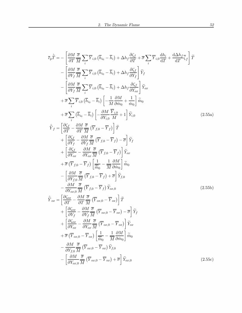
2. The Dynamic Flame 52
cp˙T = −
[∂M
∂T
σ
M
∑
i
Y i,0
(hi0 − hi
)+ ∆hf
∂ζf
∂T+ σ
∑
i
Y i,0dhi
dT+
d∆hf
dTζf
]T
−[
∂M
∂Yf
σ
M
∑
i
Y i,0
(hi0 − hi
)+ ∆hf
∂ζf
∂Yf
]Yf
−[
∂M
∂Yf
σ
M
∑
i
Y i,0
(hi0 − hi
)+ ∆hf
∂ζf
∂Yox
]Yox
+ σ∑
i
Y i,0
(hi0 − hi
) [− 1
M
∂M
∂m0+
1
m0
]˜m0
+ σ∑
i
(hi0 − hi
) [− ∂M
∂Yi,0
Y i,0
M+ 1
]Yi,0 (2.55a)
˙Y f =
[∂ζf
∂T− ∂M
∂T
σ
M
(Y f,0 − Y f
)]T
+
[∂ζf
∂Yf− ∂M
∂Yf
σ
M
(Y f,0 − Y f
)− σ
]Yf
+
[∂ζf
∂Yox− ∂M
∂Yox
σ
M
(Y f,0 − Y f
)]Yox
+ σ(Y f,0 − Y f
) [ 1
m0− 1
M
∂M
∂m0
]˜m0
−[
∂M
∂Yf,0
σ
M
(Y f,0 − Y f
)+ σ
]Yf,0
− ∂M
∂Yox,0
σ
M
(Y f,0 − Y f
)Yox,0 (2.55b)
˙Y ox =
[∂ζox
∂T− ∂M
∂T
σ
M
(Y ox,0 − Y ox
)]T
+
[∂ζox
∂Yf− ∂M
∂Yf
σ
M
(Y ox,0 − Y ox
)− σ
]Yf
+
[∂ζox
∂Yox− ∂M
∂Yox
σ
M
(Y ox,0 − Y ox
)]Yox
+ σ(Y ox,0 − Y ox
) [ 1
m0− 1
M
∂M
∂m0
]˜m0
− ∂M
∂Yf,0
σ
M
(Y ox,0 − Y ox
)Yf,0
−[
∂M
∂Yox,0
σ
M
(Y ox,0 − Y ox
)+ σ
]Yox,0 (2.55c)

2. The Dynamic Flame 53
˜H =
[∂M
∂T∆hfζf + M
d∆hf
dTζf + M ∆hf
∂ζf
∂T
]T
+
[∂M
∂Yf∆hfζf + M ∆hf
∂ζf
∂Yf
]Yf
+
[∂M
∂Yox∆hfζf + M ∆hf
∂ζf
∂Yox
]Yox
+∂M
m0∆hfζf
˜m0 +∂M
∂Yf,0∆hfζf Yf,0 +
∂M
∂Yox,0∆hfζf Yox,0 (2.55d)
wide range of behaviors depending on the manner in which M is defined.
To first gain an insight to the importance of the mass function to the flame dynamics, it is
instructive to consider several example cases. Since there are no immediately intuitive physically
motivated constraints, it is convenient to first consider the simplest and most common constraints -
constant mass and constant volume. A constant reactor volume is motivated historically by the very
first experimental well-stirred reactors that were in a porous ceramic that purposefully constrained
the reaction volume. A gas turbine combustor has no such constraint, however (particularly in the
transient sense). A constant mass reactor is desirable only because it allows gross simplification of
the expansions in Equations 2.55a through 2.55d.
Constant Mass and Constant Volume Reactors
Figure 2.13 shows the frequency responses for a methane flame with constant reactor mass across
a variety of equivalence ratios. Similarly, Figure 2.14 shows the frequency responses for a flame of
constant volume for the same set of equivalence ratios. In both cases, the flame size (be it in the
form of mass or volume) was selected to match the physical flame represented in Figures 2.2 and
2.3 as closely as possible.
Note that Figures 2.14 and 2.13 represent nearly identical systems. This is easily explained since
the only distinction between a flame of constant mass and constant volume is in the variation of
the fluid density, made clear by the relation M = ρV . That density variations are inconsequential
can be demonstrated by any number of methods from defining density as a dynamic output and
computing the transfer functions to computing the surface for steady density over the operating

2. The Dynamic Flame 54
envelope and observing that it is flat compared with other parameters. In fact, in response to a
1% change in mass flow rate, density changes on the order of 0.001%. Similarly, a 1% variation in
equivalence ratio results in perturbations on the order of 0.01%.
When compared with Figures 2.2 and 2.3, it is apparent that, consistent with results observed
in the literature, constant-size flames exhibit bandwidths extending much further than the physical
flame. Since the flow rate and flame size were all set to mimic the physical flame, it follows that
the residence time in the model is also consistent with the residence time in the physical flame.
Consequently, it must necessarily follow that the residence time in a constant reactor size model
does not obey the correct dynamics.
Critical Exhaust Constrained Reactor
One potential explanation for the expansion or contraction of the flame in the absence of a model
with spatial dependencies might be based on the exhaust properties. If the exhaust has a vast excess
of fuel and oxidizer, it stands to reason that the flame would expand to allow further combustion.
By the same token, if the exhausting fuel is extremely scarce, the reaction rate might slow and the
flame may contract. The result is that the flame might naturally expand or contract until only a
certain quantity of fuel remains.
If the exhaust fuel mass fraction is fixed to a predetermined critical value, then the steady flame
temperature is still given by inverting Equation 2.42. Given the reaction progress and temperature,
Equation 2.40predicts σ and subsequently τres. Assuming that the flame really does exhibit a
similar dynamic response to the well mixed tank described above, then the cutoff frequency would
correspond to σ/(2π). Figure 2.15 shows the predicted cutoff frequency for a critical fuel mass
fraction across a variety of equivalence ratios. Given the similarity between Figure 2.15 and the
VACCG results in Figure 2.7 it seems promising to pursue this line of reasoning.
There are, however, several points that render the critical exhaust constraint (CEC) nonphysical:
1. The use of fuel mass fraction is limited to ultra-lean cases where the depletion of oxidizer has
a negligible effect on the reaction rate,
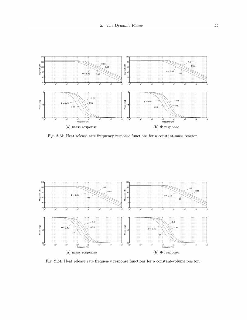
2. The Dynamic Flame 55
100
101
102
103
104
105
106
107
40
60
80
100
120
140
0.50Mag
nitu
de (
dB)
Φ = 0.45
0.55
0.60
100
101
102
103
104
105
106
107
−90
−45
0
0.50
Pha
se (
deg)
Frequency (Hz)
Φ = 0.45 0.55
0.60
100
101
102
103
104
105
106
107
0
20
40
60
80
100
0.5
Mag
nitu
de (
dB)
Φ = 0.45
0.55
0.6
100
101
102
103
104
105
106
107
−90
−45
0
0.5
Pha
se (
deg)
Frequency (Hz)
Φ = 0.45
0.55
0.6
100
101
102
103
104
105
106
107
−90
−45
0
0.5
Pha
se (
deg)
Frequency (Hz)
Φ = 0.45
0.55
0.6
(a) mass response (b) Φ response
Fig. 2.13: Heat release rate frequency response functions for a constant-mass reactor.
100
101
102
103
104
105
106
107
40
60
80
100
120
140
Φ = 0.45
Mag
nitu
de (
dB)
0.5
0.55
0.6
100
101
102
103
104
105
106
107
−90
−45
0
Φ = 0.45
Pha
se (
deg)
Frequency (Hz)
0.5
0.55
0.6
100
101
102
103
104
105
106
107
0
20
40
60
80
100
Φ = 0.45
Mag
nitu
de (
dB)
0.5
0.550.6
100
101
102
103
104
105
106
107
−90
−45
0
Φ = 0.45
Pha
se (
deg)
Frequency (Hz)
0.5
0.55
0.6
(a) mass response (b) Φ response
Fig. 2.14: Heat release rate frequency response functions for a constant-volume reactor.
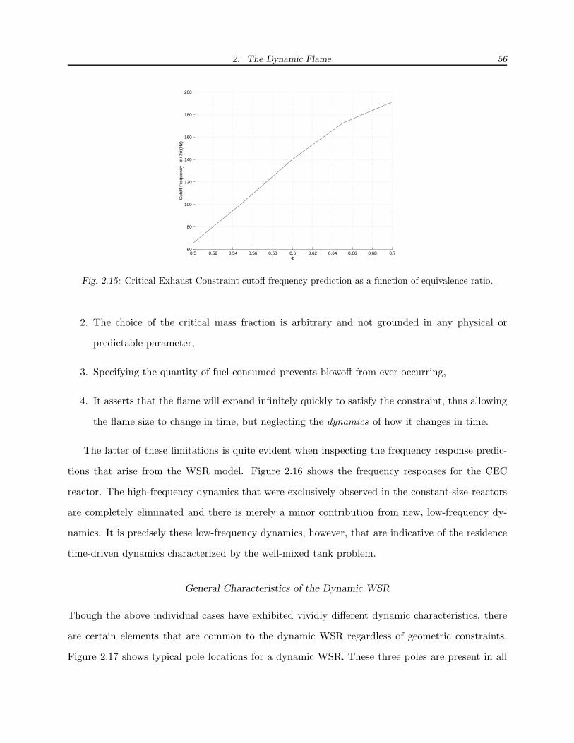
2. The Dynamic Flame 56
0.5 0.52 0.54 0.56 0.58 0.6 0.62 0.64 0.66 0.68 0.760
80
100
120
140
160
180
200
Φ
Cut
off F
requ
ency
σ
/ 2π
(Hz)
Fig. 2.15: Critical Exhaust Constraint cutoff frequency prediction as a function of equivalence ratio.
2. The choice of the critical mass fraction is arbitrary and not grounded in any physical or
predictable parameter,
3. Specifying the quantity of fuel consumed prevents blowoff from ever occurring,
4. It asserts that the flame will expand infinitely quickly to satisfy the constraint, thus allowing
the flame size to change in time, but neglecting the dynamics of how it changes in time.
The latter of these limitations is quite evident when inspecting the frequency response predic-
tions that arise from the WSR model. Figure 2.16 shows the frequency responses for the CEC
reactor. The high-frequency dynamics that were exclusively observed in the constant-size reactors
are completely eliminated and there is merely a minor contribution from new, low-frequency dy-
namics. It is precisely these low-frequency dynamics, however, that are indicative of the residence
time-driven dynamics characterized by the well-mixed tank problem.
General Characteristics of the Dynamic WSR
Though the above individual cases have exhibited vividly different dynamic characteristics, there
are certain elements that are common to the dynamic WSR regardless of geometric constraints.
Figure 2.17 shows typical pole locations for a dynamic WSR. These three poles are present in all
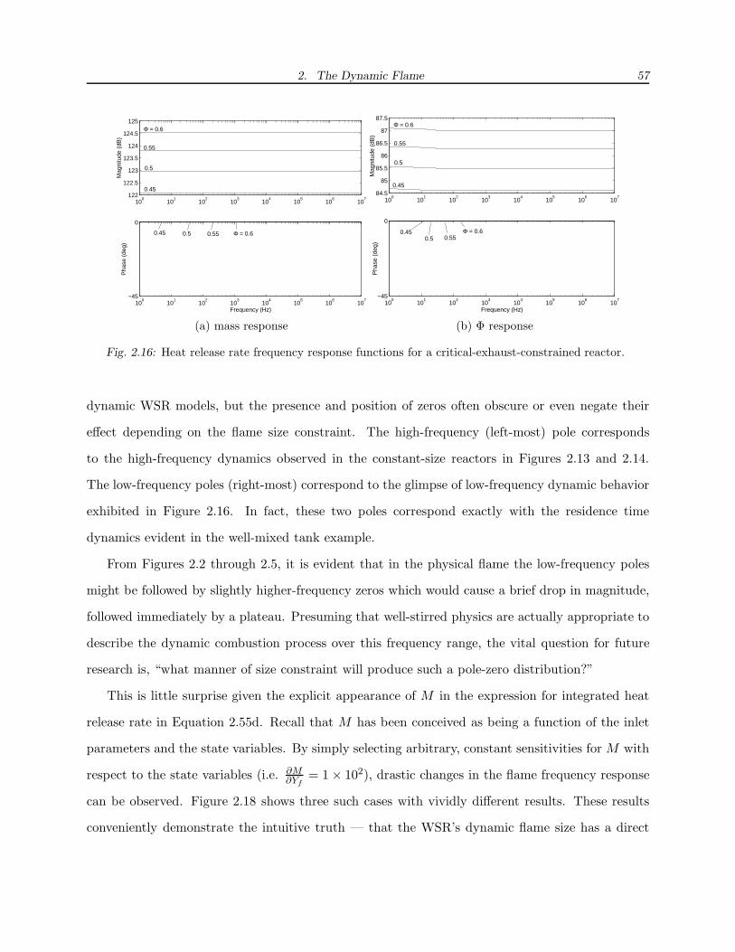
2. The Dynamic Flame 57
100
101
102
103
104
105
106
107
122
122.5
123
123.5
124
124.5
125Φ = 0.6
Mag
nitu
de (
dB)
0.55
0.5
0.45
100
101
102
103
104
105
106
107
−45
0
Φ = 0.6
Pha
se (
deg)
Frequency (Hz)
0.550.50.45
100
101
102
103
104
105
106
107
84.5
85
85.5
86
86.5
87
87.5Φ = 0.6
Mag
nitu
de (
dB)
0.55
0.5
0.45
100
101
102
103
104
105
106
107
−45
0
Φ = 0.6
Pha
se (
deg)
Frequency (Hz)
0.550.50.45
(a) mass response (b) Φ response
Fig. 2.16: Heat release rate frequency response functions for a critical-exhaust-constrained reactor.
dynamic WSR models, but the presence and position of zeros often obscure or even negate their
effect depending on the flame size constraint. The high-frequency (left-most) pole corresponds
to the high-frequency dynamics observed in the constant-size reactors in Figures 2.13 and 2.14.
The low-frequency poles (right-most) correspond to the glimpse of low-frequency dynamic behavior
exhibited in Figure 2.16. In fact, these two poles correspond exactly with the residence time
dynamics evident in the well-mixed tank example.
From Figures 2.2 through 2.5, it is evident that in the physical flame the low-frequency poles
might be followed by slightly higher-frequency zeros which would cause a brief drop in magnitude,
followed immediately by a plateau. Presuming that well-stirred physics are actually appropriate to
describe the dynamic combustion process over this frequency range, the vital question for future
research is, “what manner of size constraint will produce such a pole-zero distribution?”
This is little surprise given the explicit appearance of M in the expression for integrated heat
release rate in Equation 2.55d. Recall that M has been conceived as being a function of the inlet
parameters and the state variables. By simply selecting arbitrary, constant sensitivities for M with
respect to the state variables (i.e. ∂M∂Yf
= 1 × 10²), drastic changes in the flame frequency response
can be observed. Figure 2.18 shows three such cases with vividly different results. These results
conveniently demonstrate the intuitive truth — that the WSR’s dynamic flame size has a direct

2. The Dynamic Flame 58
-
6imag
real@@��
“Chemical” Dynamics
@@@@��
Residence TimeDynamics
Fig. 2.17: Root loci for the dynamic WSR (zeros omitted). The low-frequency coincident poles correspondto the time-constant dynamics exhibited by the well-mixed tank. The various size constraintsplace zeros in different places where they may or may not cancel with these poles.
impact on the DC gain and the zero locations, thus the flame’s dynamic response.
Without the proper constraint on its size, the WSR is incapable of capturing the appropriate
dynamics. The low-frequency, residence time-based dynamic characteristics that the WSR has the
potential to display are minimalized in simpler WSR geometric constraints, and a more appropriate
constraint is not forthcoming without first consulting more advanced models.
2.9 Flame Transfer Function
In the absence of a reliable physics-based model, it is simple enough to construct a crude first order
model that exhibits behavior consistent with the residence time dynamics. The first order transfer
functions in Equations 2.56a and 2.56b have a single pole corresponding to the residence time as a
time constant (τres = σ−1), and have DC gains calculated from Equations 2.48a and 2.48b.
Fv =Km
sτres + 1(2.56a)
FΦ =KΦ
sτres + 1(2.56b)

2. The Dynamic Flame 59
100
101
102
103
104
105
75
80
85
90
95
100
105
Mag
nitu
de (
dB)
100
101
102
103
104
105
−90
−45
0
45
Pha
se (
deg)
Frequency (Hz)
(a)(b)(c)
Fig. 2.18: Frequency response for the dynamic WSR with various arbitrary mass dependencies.(a) ∂M
∂Yf> 0, ∂M
∂Yox< 0
(b) ∂M∂Yf
> 0,
(c) ∂M∂T
< 0

3. DYNAMIC TURBULENT MIXING
The mixing model is responsible for determining the transfer function from velocity perturbations
at the injection plane to equivalence ratio perturbations at the dump plane. In the physical combus-
tor, fuel-air mixing occurs so far up stream that any such coupling is negligible if even measurable.
However, some have postulated[11] that in industrial gas turbines, where the fuel injection is fre-
quently choked and injected nearer the flame, since velocity perturbations in the air will not result
in corresponding velocity perturbations in the choked fuel rich and lean pockets may propagate
downstream to the flame.
In the experimental combustor and in industrial systems, the length separating the injection
location from the flame, depicted in Figure 3.1, the flow is highly turbulent. The quality of the
mixing in this region determines whether or not mixing perturbations will have a significant effect
on the flame. Poor mixing will allow the rich and lean pockets to retain their concentrations, while
good mixing will result in a more even fuel-air distribution, preventing “high”-frequency mixing
perturbations from being delivered to the flame.
-Air In
@@ @@ @@ @@ @@ @@ @@ @@ @@ @@ @@ @@ @@ @@ @@ @@ @@ @@ @@ @@
@@ @@ @@ @@ @@ @@ @@ @@ @@ @@ @@ @@ @@ @@ @@ @@ @@ @@ @@
Flame
-Dump Plane
-Exit Plane
?
Fuel In
Injection Plane
Fig. 3.1: A conceptual combustor burning premixed fuel-air. Repeated from Figure 1.3.
3. Dynamic Turbulent Mixing 61
3.1 Stochastic Mixing
The model used in this effort was developed by William Baumann et. al. of the VACCG, and
was based on a previous work by Scarinci and Freeman[24], which treated turbulent diffusion as a
purely stochastic process. The entire model is based on the premise that any given particle will
deviate in location from that of the mean flow by a distance governed by a Gaussian Probability
Distribution. Therefore, in a one-dimensional system, the probability distribution in probability
per unit length, Q, that a particle beginning at a position x′ at time t′ will arrive at a position x
at time t > t′ is given by
Q(x, t|x′, t′) =1√
2πσx2
exp
{− [x − x′ − U · (t − t′)]2
2σx2
}, (3.1)
where U is the mean velocity, and σx is the standard deviation on x which will be discussed later.
Let the function, S(x, t), describe the injection of fuel in moles per unit time per unit length.
This general realization allows for the arbitrary injection of fuel over space as a function of time.
For every unit of fuel injected into the system, its expected concentration (in moles per unit length)
is identically equal to its probability distribution (in probability per unit length). This notion may
be expanded to apply to the continuous injection of particles anywhere in the system at all points
in time. In this sense, Q can be integrated with S over all points in space and time, x′ and t′ at
which particles were injected to obtain the concentration in particles per unit length at x and t
thusly:
C(x, t) =
∫∞
−∞
∫ t
0Q(x, t|x′, t′)S(x′, t′)dt′dx′. (3.2)
In this sense, Q is a mapping describing the fraction of particles that migrate from the points, (x′, t′)
at which they are injected to points (x, t). Thanks to the integrals, the function, C, is inclusive
of the total migration of all injected particles over all space and elapsed time to the location x at
time t.
This general realization may now be simplified to describe the combustor. If the injection plane

3. Dynamic Turbulent Mixing 62
is at x = −xi, and the dump plane is at x = 0, then the injection function must be given by
S(x, t) = δ(x + xi)s(t),
where s(t) is rate of fuel injection in moles per unit time at the injection plane. This allows Equation
3.2 to be conveniently simplified to
C(x, t) =
∫ t
0Q(x, t|xi, t
′)s(t′)dt′. (3.3)
Conveniently, this realization results in a dynamic system exhibiting a linear response at all
points in space. If the input is expressed as the linear combination of two functions, s(t) =
af(t) + bg(t), then
C(x, t) =
∫ t
0Q(x, t|xi, t
′)(af(t′) + bg(t′)
)dt′
= a
∫ t
0Q(x, t|xi, t
′)f(t′)dt′ + b
∫ t
0Q(x, t|xi, t
′)g(t′)dt′,
so the response will be the linear combination of the component responses—the definition of a
linear response.
3.2 The Random Walk and Diffusivity
The problem of the diffusion of particles is analogous to the random walk problem. If a group
of individuals begin at the same point in space and take a series of steps of random size and
direction, their paths will ultimately diverge from one another. The phenomenon can be shown to
be a convenient example of linear diffusivity — one in which the variance of the position of each
individual grows linearly in time[2].
If this same principle is applied to the diffusion of molecules in a turbulent flow, a similar result
can be achieved. Let the velocity for the turbulent mixture be given by ui = U + vi, where ui
is the total velocity of a single particle,U is the bulk or mean velocity, and vi the unsteady and
3. Dynamic Turbulent Mixing 63
random turbulent velocity, which is unique for each particle regardless of its position. Therefore an
individual particle’s divergence from the bulk flow after having been injected at t = 0, xi, is given
by
xi(t) =
∫ t
0
(ui(t
′) − U(t′))dt′ =
∫ t
0vi(t
′)dt′. (3.4)
Therefore, the variance of the particle deviation is given by
σx2 =
1
N
N∑
i=1
xi2 =
1
N
N∑
i=1
(∫ t
0vi(t
′)dt′)·(∫ t
0vi(t
′′)dt′′)
.
Simply by manipulating the integrals, this can be simplified to
σx2 =
1
N
N∑
i=1
∫ t
0
∫ t
0vi(t
′) · vi(t′′)dt′dt′′.
As N becomes very large (as in the spirit of the continuum assumption), the quantity,
1/N∑N
i=1 vi(t′) · vi(t
′′) approaches the the expected value of the multiple of the two velocities.
Therefore,
σx2 =
∫ t
0
∫ t
0
⟨vi(t
′) · vi(t′′)⟩dt′dt′′. (3.5)
The trouble remains to compute 〈v(t′) · v(t′′)〉. Called the auto-velocity correlation, this is the
correlation between the sets of velocities at two points in time. When t′ = t′′, the set of velocities are
identical and the correlation can be shown to be identically v2 or the average turbulence intensity.
Much can be said on the computation and measurement of this quantity as the times diverge [4],
but it is sufficient to estimate that the velocity auto correlation decays like
⟨vi(t
′) · vi(t′′)⟩
= v2 exp
(−|t′′ − t′|
τ
), (3.6)
where τ is the empirically obtained turbulence timescale, and v2 is the turbulence intensity. By
substituting into Equation 3.5, the integrals become feasible to evaluate. Thanks to the symmetry
3. Dynamic Turbulent Mixing 64
of Equation 3.2, the discontinuity along the line where t′′ = t′ can be dealt with simply by evaluating
the integral on one side of the line and doubling the result thusly
σx2 = 2
∫ t
0
∫ t′′
0v2 exp
(−|t′′ − t′|
τ
)dt′dt′′ = 2v2τ [t − τ exp(−t/τ) + τ ] .
Although this result is undesirably nonlinear, so long as the turbulence time scales are very
small relative to the convective time scale (which will be discussed later), the variance describing
the spatial distribution of particles injected at t = 0 becomes simply
σx2 = 2v2τt. (3.7)
Equation 3.7 reflects the much celebrated result that for sufficiently fast turbulent time scales,
turbulent diffusion is linear.
3.3 Mixing Frequency Response
In order to capitalize on this result in the current effort, however, this information must be used to
describe a transfer function between mixture perturbations at the injection plane and their effect
at the dump plane. The output of the mixing model must, therefore, be the equivalence ratio at
the dump plane (where x = 0), while the input is the rate of dynamic injection of fuel particles at
the inlet.
Since the system is linear, its transfer function can be found as the transform of the impulse
response. If s(t′) = δ(t′), the fuel concentration at the dump plane in moles per unit length, C(0, t),
is given by
Cδ(0, t) =
∫ t
0Q(0, t|xi, t
′)δ(t′)dt′
=1√
2πσx2
exp
{−(xi − Ut)2
2σx2
}. (3.8)
3. Dynamic Turbulent Mixing 65
−1.5 −1 −0.5 0 0.5 10
1
2
3
4
5
6
x/xi
Conc
entra
tion
(mol
es/m
)Dump Plane Injection Plane
Fig. 3.2: Fuel concentration in mol/m plotted over normalized position for three points in time with arbitraryvalues of U , v2, and xi.
Therefore, the transfer function, M , is given by
M(jω) = F {Cδ(0, t)}
=
∫∞
−∞
exp(−jωt)1√
2πσx2
exp
{−(xi − Ut)2
2σx2
}dt. (3.9)
Though cumbersome to evaluate analytically, this is quite trivial to compute numerically since most
software packages have Fourier analysis tools built in. Though it is disappointing not to have an
explicit algebraic solution for the mixing transfer function, it is possible to derive a number of key
parameters from Equation 3.9.
Figure 3.2 shows the concentration as a function of x at various points in time after the injection
for some arbitrary values of the relevant variables. It is easy to see that there is some characteristic
delay before the pulse reaches the dump plane. Also, it is intuitive that the degree to which the
pulse has diffused when it reaches the dump plane will depend on the turbulence level and the time
over which it has been exposed to the turbulence before reaching the dump plane.
3. Dynamic Turbulent Mixing 66
0 0.05 0.1 0.15 0.2 0.25 0.3 0.35 0.40
0.5
1
1.5
2
2.5
3
time (seconds)
Con
cent
ratio
n (m
oles
/m)
Fig. 3.3: The mixing impulse response at the dump plane in mol/m with arbitrary values of U , v2, and xi.
Figure 3.3 shows the response as a function of time at the dump plane. It is worth noting that
though it is difficult to observe in Figure 3.3, the time response if asymmetric about the peak. This
is easily explained by observing in Figure 3.2 that as the pulse passes the dump plane, it continues
to grow more diffuse, so that the time response will decline more slowly than it grows.
Since it is the Fourier transform of this curve that indicates the frequency response, it is intuitive
that preservation of the shape of this curve will also preserve the predominant characteristics of
the frequency response. Figure 3.4 shows the magnitude and phase of the transfer function from
the injection function to the concentration computed from Figure 3.3. There are three primary
characteristics that describe the transfer function: DC gain, bandwidth, and delay.
1. Delay. The simplest to interpret, the delay is indicated by the appearance of a nearly linear
phase lag in the frequency response. The dotted line in Figure 3.4(b) indicates the phase lag
that would correspond to the delay between the instant of injection and the instant the peak

3. Dynamic Turbulent Mixing 67
100
101
102
−200
−180
−160
−140
−120
−100
−80
−60
−40
−20
0
frequency (Hz)
Mag
nitu
de (
dB)
0 10 20 30 40 50 60 70 80 90 100−8000
−7000
−6000
−5000
−4000
−3000
−2000
−1000
0
frequency (Hz)
Pha
se (
deg)
Mixing DelayConvective Delay
(a) (b)
Fig. 3.4: The mixing frequency response computed from Figure 3.3.
reaches the dump plane. Called the convection time, this quantity is given by
τconv =xi
U.
The phase deviates from the dotted line because the response at the dump plane necessarily
becomes significant before the arrival of the peak to a degree depending on how well diffused
the pulse is as it crosses the dump plane. Regardless, the convective delay is a convenient
time scale with which to characterize the system. Though the actual exhibited delay will
vary somewhat as other parameters change, the convective delay is a reasonable estimator for
the total mixing delay, indicating that if τconv is conserved, the mixing delay will be nearly
conserved.
2. DC Gain. The DC gain can be determined completely from static principles. Given a static
molar rate of fuel injection in mol/s, s, the resulting concentration at the dump plane will be
s/U . Therefore, the DC gain of the transfer function between fuel injection and concentration
at the dump plane is simply 1/U .
3. Bandwidth. The bandwidth is determined entirely by the shape of the curve depicted in

3. Dynamic Turbulent Mixing 68
Figure 3.3. The more diffuse the curve, the lesser the influence high-frequency components,
the lower the bandwidth becomes. The shape of the curve is crudely estimated as Gaussian
distribution in time rather than space, though it has already been established that the re-
sponse is not Gaussian in time (only in space). That counter-argument not withstanding, the
variance in the time domain can be estimated as the variance in space at the instant when
the peak passes through the dump plane, adjusted by the speed at which it passes the dump
plane, so that
σt2 ≈ σx
2(τconv)
U2= 2
τxiv2
U3. (3.10)
Figure 3.5 shows the frequency corresponding to a -3dB drop in magnitude for conditions
spanning values of U from 1 to 10m/s, v2 from 2 to 20m2/s2, and xi from 0.1 to 1m, plotted
against corresponding values of σt. Clearly, over this very physically viable range of parameters,
Fcutoff · σt ≈ 0.13, (3.11)
where F is in Hz, is an excellent correlation. In fact, the only time this very simple relationship
breaks down is when the ratio, U2/v2 becomes quite small (∼ 10−5). Since neglecting additional
diffusion of the peak as it progresses through the dump plane is an inherent assumption for the
estimate of σt, when the turbulence intensity dominates the mean velocity so strongly, making
progression of the peak slow relative to its diffusion, Equation 3.10 is invalid. However, it is a
rare case, indeed, when the turbulence intensity is even four orders of magnitude greater than the
square of the mean velocity.
3.4 Validation
In order to validate the model, the physical transfer function was measured as follows. A dynamic
“on-off” valve allowed the superimposition of a low-amplitude, rapid (≤500Hz) injection of fuel
onto the typical steady fuel-air mixture. A laser absorption technique facilitated the dynamic
3. Dynamic Turbulent Mixing 69
10−4
10−3
10−2
10−1
100
10−1
100
101
102
103
104
σt (sec)
f cuto
ff (H
z)F
cutoff σ
t ≈ 0.13
Fig. 3.5: Mixing transfer function cutoff frequency as a function of the σt estimate in Equation 3.10
measurement of fuel concentrations at two points downstream of the dynamic injection point. In
this scenario, empirical transfer functions are calculable from the known fuel injection functions,
and the measured downstream concentration functions. Figure 3.6 shows the measured magnitude
response for the two positions compared with the model predictions for the same locations. The
agreement between them is amply sufficient to warrant application of the model.
3.5 Establishing the Proper Units
Recall that the mixing transfer function describes the response in equivalence ratio at the dump
plane with respect to velocity perturbations in the air stream at the injection plane. Thus far, the
input has consistently been the injection of fuel and the output has been fuel concentration at the
dump plane.
The equivalence ratio local to the injection plane can be expressed as
Φ =Nf/Na
β,
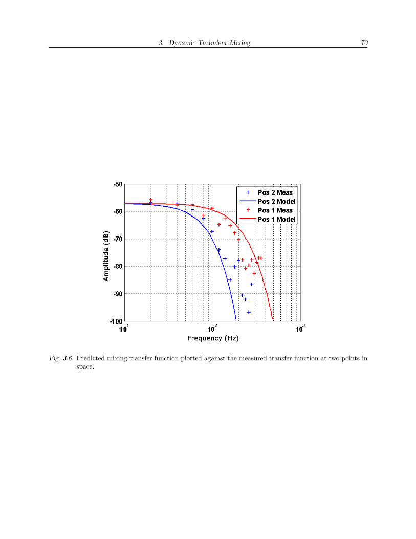
3. Dynamic Turbulent Mixing 70
Fig. 3.6: Predicted mixing transfer function plotted against the measured transfer function at two points inspace.
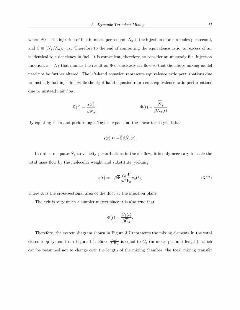
3. Dynamic Turbulent Mixing 71
where Nf is the injection of fuel in moles per second, Na is the injection of air in moles per second,
and β ≡ (Nf/Na)stoich. Therefore to the end of computing the equivalence ratio, an excess of air
is identical to a deficiency in fuel. It is convenient, therefore, to consider an unsteady fuel injection
function, s = Nf that mimics the result on Φ of unsteady air flow so that the above mixing model
need not be further altered. The left-hand equation represents equivalence ratio perturbations due
to unsteady fuel injection while the right-hand equation represents equivalence ratio perturbations
due to unsteady air flow.
Φ(t) =s(t)
βNa
Φ(t) =Nf
βNa(t)
By equating them and performing a Taylor expansion, the linear terms yield that
s(t) ≈ −ΦβNa(t).
In order to equate Na to velocity perturbations in the air flow, it is only necessary to scale the
total mass flow by the molecular weight and substitute, yielding
s(t) ≈ −βΦρaA
MWaua(t), (3.12)
where A is the cross-sectional area of the duct at the injection plane.
The exit is very much a simpler matter since it is also true that
Φ(t) =Cf (t)
βCa
.
Therefore, the system diagram shown in Figure 3.7 represents the mixing elements in the total
closed loop system from Figure 1.4. Since ρaAMWa
is equal to Ca (in moles per unit length), which
can be presumed not to change over the length of the mixing chamber, the total mixing transfer
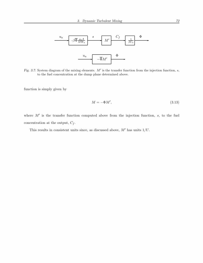
3. Dynamic Turbulent Mixing 72
-ua
-βΦ ρaAMWa
-s
M ′ -Cf
1βCa
-Φ
-ua
−ΦM ′ -Φ
Fig. 3.7: System diagram of the mixing elements. M ′ is the transfer function from the injection function, s,to the fuel concentration at the dump plane determined above.
function is simply given by
M = −ΦM ′, (3.13)
where M ′ is the transfer function computed above from the injection function, s, to the fuel
concentration at the output, Cf .
This results in consistent units since, as discussed above, M ′ has units 1/U .

4. ACOUSTICS
The acoustic transfer functions are responsible for describing the flow-field’s velocity response to
dynamic heat release rate perturbations at the flame. As discussed in the Methodology, Section
1.3, there are two locations where the acoustic response is of interest: at the dump plane where it
will drive the flame directly, and at the injection plane where it will drive the mixing described in
Chapter 3 and depicted in Figure 4.1. This portion of the work was performed by Paul Black, and
needs only be described to the extent that it is pertinent to the other sections of this document.
Though the details of how are irrelevant to this brief discussion on the acoustic model, the fluid
equations of motion in a single-dimensional duct can be written from Equations 2.4, 2.7, 2.9, and
the integral form of the momentum equation (which was omitted from the flame discussion because
-Air In
@@ @@ @@ @@ @@ @@ @@ @@ @@ @@ @@ @@ @@ @@ @@ @@ @@ @@ @@ @@
@@ @@ @@ @@ @@ @@ @@ @@ @@ @@ @@ @@ @@ @@ @@ @@ @@ @@ @@
Flame
-Dump Plane
-Exit Plane
?
Fuel In
Injection Plane
Fig. 4.1: A conceptual combustor burning premixed fuel-air. Repeated from Figure 1.3
4. Acoustics 74
it was not necessary to the discussion) as
Dρ
Dt= ρ
∂u
∂x+
ρu
A
∂A
∂x, (4.1a)
Du
Dt= −1
ρ
∂p
∂t, (4.1b)
cpDT
Dt=
1
ρ
∂p
∂t+
1
ρA
(q′ + ρA
∑
i
hiζi
). (4.1c)
Together with the ideal gas law, these equations can be linearized to form the classic acoustic
equations with two additions: the appearance of q′ and ρA∑
i hiζi, which represent the rate of
heat addition through the duct walls per unit length and heat release rate per unit length by
chemical reaction respectively (the latter defined for the WSR in Equation 2.18).
As discussed in Section 2.1, the flame is quite small relative to the length scales relevant to the
acoustics. Therefore, it is convenient to consider the flame as a point heat source, so that
ρA∑
i
hiζi = δ(x − xf )Q, (4.2)
where δ is the Kroniker Delta, xf is the position of the flame, and Q = M∑
i hiζi is the heat release
rate from the flame, established in Equation 2.18.
Having now established the mode of excitation, the various important geometric constraints
were entered in AbacusTM. The difficulty of this effort is not to be under emphasized by the
brevity of its discussion in this document. That the details of producing the acoustic model are
omitted is a testament not to the unimportance of the task, rather to the depth and magnitude of
the distraction it would provide from its impact on the stability model.
These models were produced to describe the velocity responses at the dump plane and the injec-
tion plane to perturbations in flame heat release rate for two geometries: the original experimental
combustor and a lengthened combustor. The motivation for these two geometries will be made
clear in Chapter 5. The results appear as magnitude and phase as a function of frequency.
Figures 4.2 and 4.3 show the original combustor response and the modified combustor response
respectively. Important features to note are the slightly elevated low-frequency magnitudes in the

4. Acoustics 75
100
101
102
103
−200
−180
−160
−140
−120
−100
Mag
nitu
de (
dB)
100
101
102
103
−400
−300
−200
−100
0
Pha
se (
deg)
Frequency (Hz)
100
101
102
103
−180
−160
−140
−120
−100
−80
Mag
nitu
de (
dB)
100
101
102
103
−600
−500
−400
−300
−200
−100
0
Pha
se (
deg)
Frequency (Hz)
(a) (b)
Fig. 4.2: Original, open-to-atmosphere combustor acoustics. Magnitude units are in m/J . Plot (a) representsthe response at the dump plane and (b) represents the response at the injection plane.
latter, shift in the 90◦ phase lag from about 500Hz in the unmodified combustor to roughly 200Hz in
the modified combustor. In Chapter 5 it will be established that these factors combine to drastically
reduce the combustor’s stability.
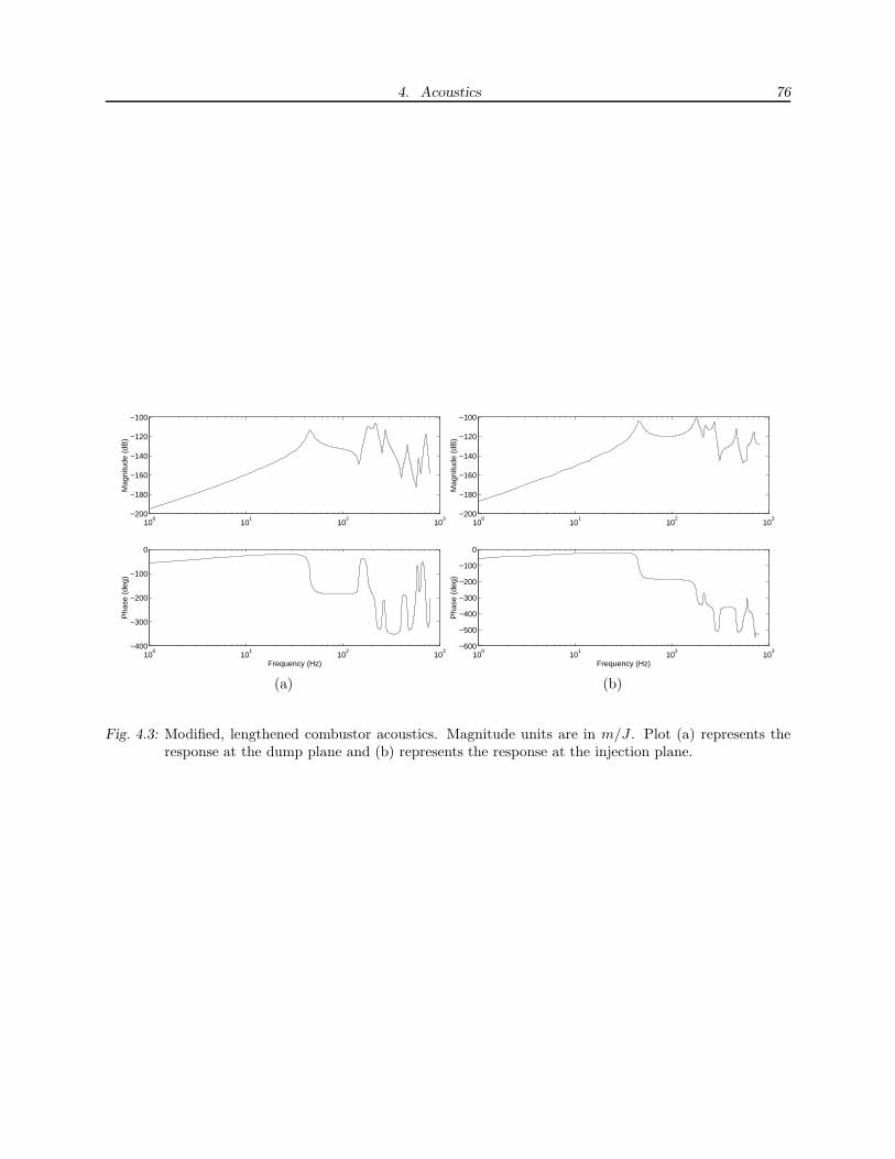
4. Acoustics 76
100
101
102
103
−200
−180
−160
−140
−120
−100
Mag
nitu
de (
dB)
100
101
102
103
−400
−300
−200
−100
0
Pha
se (
deg)
Frequency (Hz)
100
101
102
103
−200
−180
−160
−140
−120
−100
Mag
nitu
de (
dB)
100
101
102
103
−600
−500
−400
−300
−200
−100
0
Pha
se (
deg)
Frequency (Hz)
(a) (b)
Fig. 4.3: Modified, lengthened combustor acoustics. Magnitude units are in m/J . Plot (a) represents theresponse at the dump plane and (b) represents the response at the injection plane.

5. SYSTEM-LEVEL STABILITY PREDICTIONS
As established in the previous chapters, there are a number of steady parameters on which the
dynamic behavior of the various component models depends. The tool most immediately useful
for design of new systems or even operation of existing ones is a stability contour in indicating
the boundary between stable operating conditions and unstable operating conditions in parameter
space. Design engineers could perceivably use such a tool to predict the effect of physical changes
in the combustor on stability margins. Operators could perceivably use the same tool as a non-
exhaustive means for mapping the stability for a particular machine.
5.1 Classical Thermo-Acoustic Stability
The classic condition for thermo-acoustic instability was dubbed the Rayleigh criterion for the
man who first phrased it. Lord Rayleigh noted the following in his survey of thermally driven
instabilities:
“If heat be given at the moment of greatest condensation, or be taken from it at the
moment of greatest rarefaction, the vibration is encouraged. On the other hand, if heat
be given at the moment of greatest rarefaction, or abstracted at the moment of greatest
condensation, the vibration is discouraged.”[23]
More modern applications of this criterion, particularly as described by Culick’s most excellent
communication on the matter[3], have produced the mathematical criterion with the same implica-
tions. As Culick describes, the heat addition will add energy to the acoustics at a rate proportional
to p′q′, where p′ is the acoustic pressure and q′ is the unsteady rate of heat addition. Therefore,
the net addition of energy to the acoustic system is found byintegrating the interactions over all
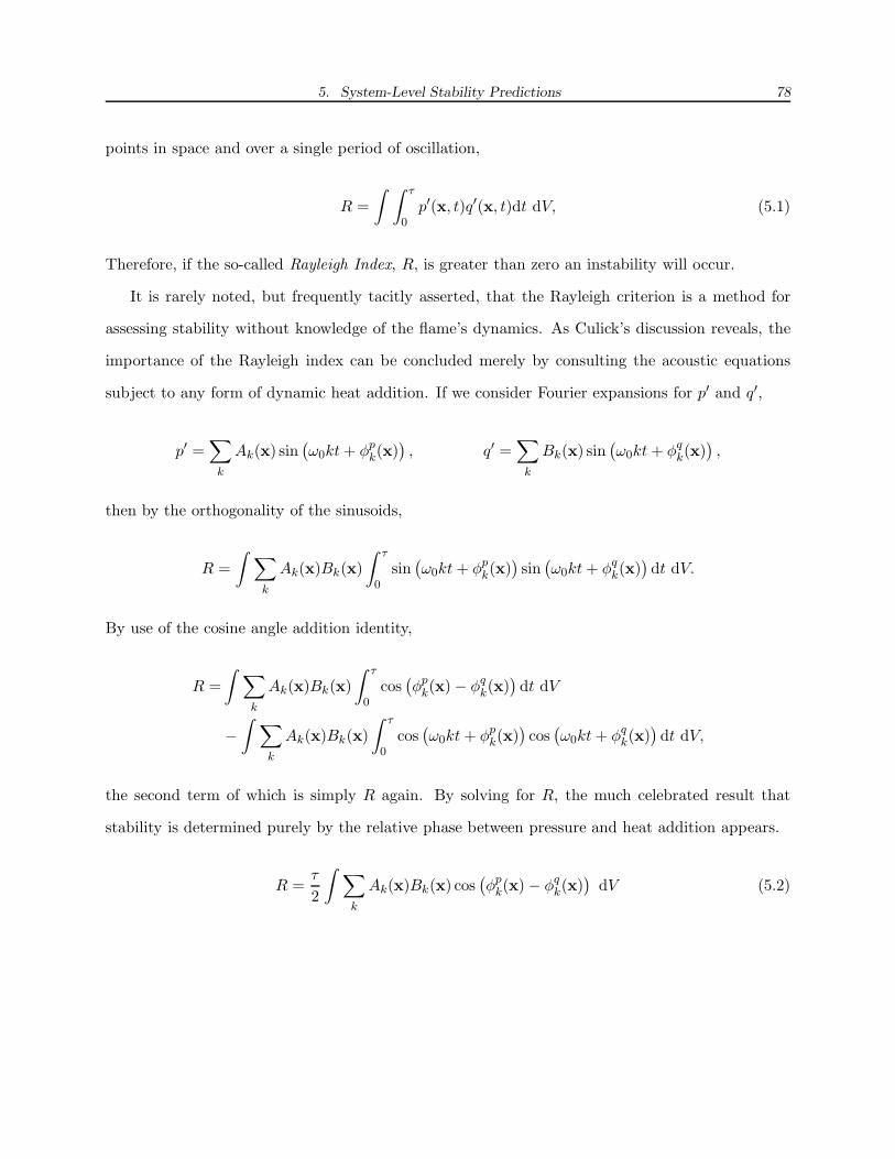
5. System-Level Stability Predictions 78
points in space and over a single period of oscillation,
R =
∫ ∫ τ
0p′(x, t)q′(x, t)dt dV, (5.1)
Therefore, if the so-called Rayleigh Index, R, is greater than zero an instability will occur.
It is rarely noted, but frequently tacitly asserted, that the Rayleigh criterion is a method for
assessing stability without knowledge of the flame’s dynamics. As Culick’s discussion reveals, the
importance of the Rayleigh index can be concluded merely by consulting the acoustic equations
subject to any form of dynamic heat addition. If we consider Fourier expansions for p′ and q′,
p′ =∑
k
Ak(x) sin(ω0kt + φp
k(x)), q′ =
∑
k
Bk(x) sin(ω0kt + φq
k(x)),
then by the orthogonality of the sinusoids,
R =
∫ ∑
k
Ak(x)Bk(x)
∫ τ
0sin(ω0kt + φp
k(x))sin(ω0kt + φq
k(x))dt dV.
By use of the cosine angle addition identity,
R =
∫ ∑
k
Ak(x)Bk(x)
∫ τ
0cos(φp
k(x) − φqk(x)
)dt dV
−∫ ∑
k
Ak(x)Bk(x)
∫ τ
0cos(ω0kt + φp
k(x))cos(ω0kt + φq
k(x))dt dV,
the second term of which is simply R again. By solving for R, the much celebrated result that
stability is determined purely by the relative phase between pressure and heat addition appears.
R =τ
2
∫ ∑
k
Ak(x)Bk(x) cos(φp
k(x) − φqk(x)
)dV (5.2)

5. System-Level Stability Predictions 79
In the case of the system described herein, however, the combustor is described by a one-
dimensional geometry and the flame is assumed to exist at a point, so
Ak(x) = akδ(x − xflame), Bk(x) = bkδ(x − xflame).
Thus, the Rayleigh Index can be simplified to
R =τ
2
∑
k
akbk cos(φp
k − φqk
). (5.3)
Equation 5.3 indicates that modes of oscillation that result in the phase difference between the
pressure and the heat release rate being −π2 < φp
k − φqk < π
2 encourage instability. This imposes no
conditions on the amplitudes of oscillation (save that they be nonzero).
The limitations of such realizations of the Rayleigh Index are found in the original formulation
of Equation 5.1, which stems from analysis on the acoustic system only. It is the notion that the
acoustic system can be reduced to an oscillator equation
η + ωn2η = Fq,
the addition of energy to which for a single period is given by∫ τ
0 ηFqdt, that allows the Rayleigh
Index to be calculated [3]. In fact, the criterion can be modified to include damping, but its
evaluation becomes quite cumbersome. Fortunately, supposing that the acoustics are characterized
by an undamped oscillator, it is possible to arrive at exactly the same condition as in Equation
5.3 using the classical systems theory that will be discussed in the following sections, but without
being impeded by the addition of damping or other complications.
5.2 Assessing Stability
While it is quite helpful to have a widely accepted criterion for the stability of a thermo-acoustic
system, once a system-level model with scalar signals is available, the Rayleigh Index is merely
redundant with more general and more easily applied methods for assessing stability. Some of

5. System-Level Stability Predictions 80
the most common classical methods for assessing stability include Laplace Domain analysis, Bode
stability criterion, and the Nyquist Criterion.
Though Laplace Domain analysis allows explicit root locus calculation, simultaneously provid-
ing stability information as well as the predominant frequencies and readily quantifiable margins
for secondary instabilities, there are a number of numerical considerations that discourage its em-
ployment in this endeavor. Firstly, though the acoustic and mixing transfer functions are defined in
the frequency domain using the methods described in the previous chapters, they do not necessarily
have readily available expression in the Laplace Domain. In order to ensure that a Laplace Domain
transfer function is available for each of the sub-systems, each frequency response would have to be
curve fitted with a Laplace Domain realization. While this is not in and of itself a daunting task,
the prevalence of delay in the mixing transfer function renders it numerically cumbersome since
there is no exact polynomial expression for delay native to the Laplace Domain. Attempts to simply
estimate the delay with high-order polynomials (in addition to the polynomials already inherent
to the acoustic and mixing dynamics) simply result in a system so numerically cumbersome that
most conventional tools lose numerical reliability.
Direct analysis of the transfer functions through the Nyquist or Frequency Domain analysis
has the benefits of being computationally unimposing, avoiding accuracy-limiting estimations, and
requiring almost no analysis prior to use in the model (as would be required to determine Laplace
Domain estimates). Since the Nyquist Criterion is the more difficult of the two to evaluate in
software, it is only natural that the stability analysis should be conducted using the Bode Criterion.
Applying the Bode Criterion
Figure 5.1 shows the total thermo-acoustic system subject to an arbitrary disturbance input. This
could be turbulent noise, ambient acoustic disturbances, or any number of perturbations to the
flow. The transfer function from the disturbance, d, to the heat release rate, q, is given by
q
d=
Fv
1 − (FvAv + FΦAΦM). (5.4)
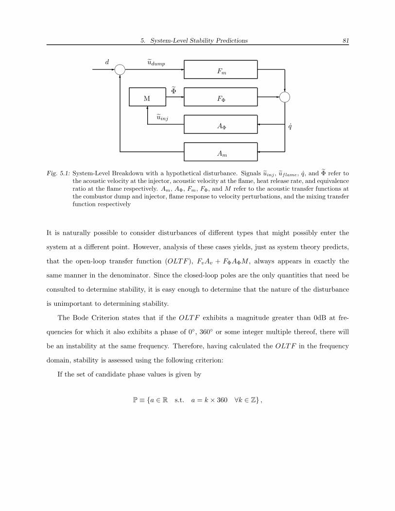
5. System-Level Stability Predictions 81
Am
6� ��
--
AΦ
6
udumpd
Fm
?
� ��
�
�q
FΦ-
M-
uinj
Φ
Fig. 5.1: System-Level Breakdown with a hypothetical disturbance. Signals uinj , uflame, q, and Φ refer tothe acoustic velocity at the injector, acoustic velocity at the flame, heat release rate, and equivalenceratio at the flame respectively. Am, AΦ, Fm, FΦ, and M refer to the acoustic transfer functions atthe combustor dump and injector, flame response to velocity perturbations, and the mixing transferfunction respectively
It is naturally possible to consider disturbances of different types that might possibly enter the
system at a different point. However, analysis of these cases yields, just as system theory predicts,
that the open-loop transfer function (OLTF ), FvAv + FΦAΦM , always appears in exactly the
same manner in the denominator. Since the closed-loop poles are the only quantities that need be
consulted to determine stability, it is easy enough to determine that the nature of the disturbance
is unimportant to determining stability.
The Bode Criterion states that if the OLTF exhibits a magnitude greater than 0dB at fre-
quencies for which it also exhibits a phase of 0◦, 360◦ or some integer multiple thereof, there will
be an instability at the same frequency. Therefore, having calculated the OLTF in the frequency
domain, stability is assessed using the following criterion:
If the set of candidate phase values is given by
P ≡ {a ∈ R s.t. a = k × 360 ∀k ∈ Z} ,
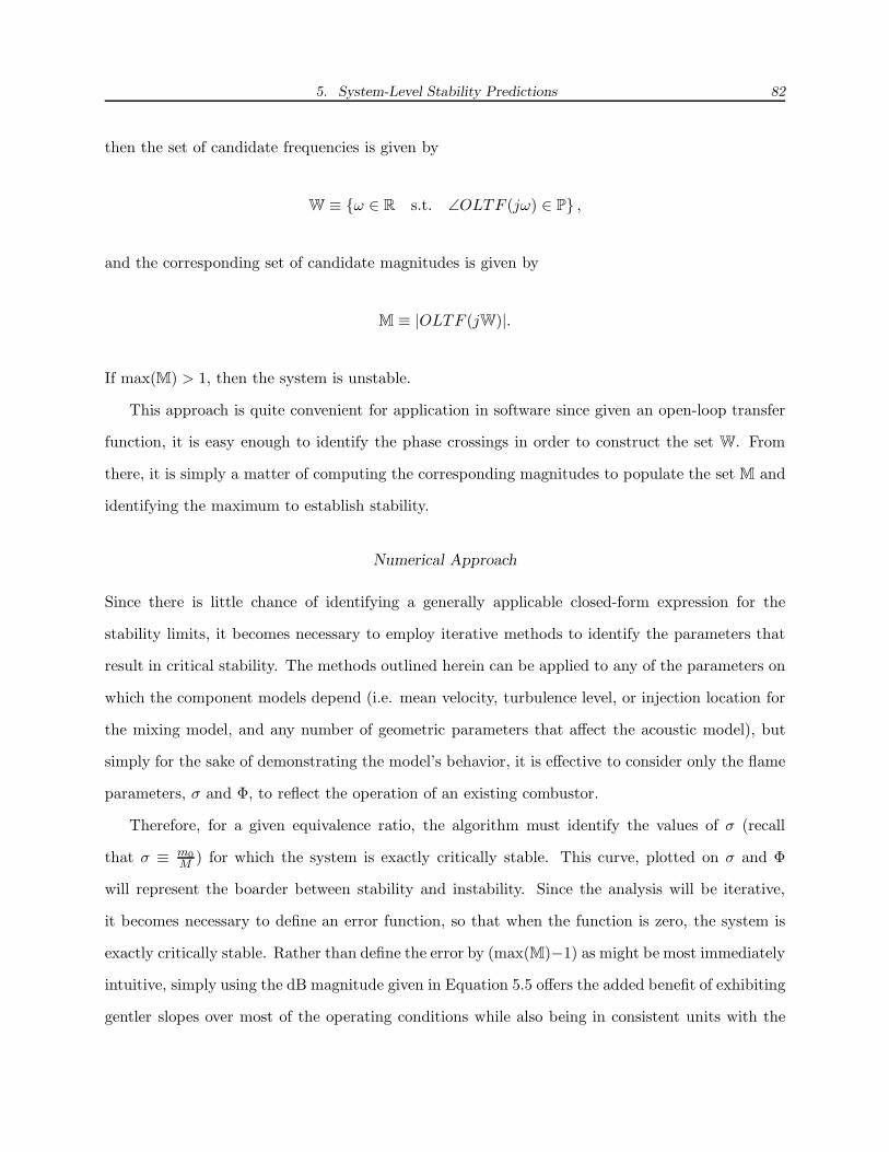
5. System-Level Stability Predictions 82
then the set of candidate frequencies is given by
W ≡ {ω ∈ R s.t. ∠OLTF (jω) ∈ P} ,
and the corresponding set of candidate magnitudes is given by
M ≡ |OLTF (jW)|.
If max(M) > 1, then the system is unstable.
This approach is quite convenient for application in software since given an open-loop transfer
function, it is easy enough to identify the phase crossings in order to construct the set W. From
there, it is simply a matter of computing the corresponding magnitudes to populate the set M and
identifying the maximum to establish stability.
Numerical Approach
Since there is little chance of identifying a generally applicable closed-form expression for the
stability limits, it becomes necessary to employ iterative methods to identify the parameters that
result in critical stability. The methods outlined herein can be applied to any of the parameters on
which the component models depend (i.e. mean velocity, turbulence level, or injection location for
the mixing model, and any number of geometric parameters that affect the acoustic model), but
simply for the sake of demonstrating the model’s behavior, it is effective to consider only the flame
parameters, σ and Φ, to reflect the operation of an existing combustor.
Therefore, for a given equivalence ratio, the algorithm must identify the values of σ (recall
that σ ≡ m0
M) for which the system is exactly critically stable. This curve, plotted on σ and Φ
will represent the boarder between stability and instability. Since the analysis will be iterative,
it becomes necessary to define an error function, so that when the function is zero, the system is
exactly critically stable. Rather than define the error by (max(M)−1) as might be most immediately
intuitive, simply using the dB magnitude given in Equation 5.5 offers the added benefit of exhibiting
gentler slopes over most of the operating conditions while also being in consistent units with the

5. System-Level Stability Predictions 83
transfer function plots.
E(σ,Φ) = 20log10
(max (M(σ,Φ))
)(5.5)
The algorithm to identify and compute these critical stability conditions proceeds as follows:
1. Select a value for Φ (selecting Φ as opposed to σ is an arbitrary choice).
2. Compute σblowoff (Φ) using the criterion in Equation 2.46.
3. Compute E for a set of values for σ between 0 and σblowoff and identify zero crossings.
4. For each zero crossing, use the value for σ on either side of the crossing as initial guesses for
secant iteration to compute the critical σ.
By first computing the entire range of σ values from the stagnant flame to blowoff, the algorithm
can identify the appearance of stability “pockets” that might have otherwise been overlooked using
other numerical approaches.
5.3 Stability Characteristics
It is first worth noting that not all combustors are likely to exhibit a dynamic mixing response
either since the injection may not be choked or might be so well mixed as to exhibit a negligible
frequency response. For this reason, it is of interest to observe the roles of velocity coupling only
as well as Φ and velocity coupling together. Therefore, the two open-loop transfer functions that
might describe an arbitrary combustor to which the assumptions outlined in each of the component
sections applies are FmAm and FmAm + FΦAΦM .
Instability Due to Velocity Coupling Alone
When the open-loop transfer function is given by FmAm, since the acoustic transfer function is
independent of the equivalence ratio and mass flow (assuming low Mach-number flow), Fm bears
5. System-Level Stability Predictions 84
0 0.1 0.2 0.3 0.4 0.5 0.6 0.7 0.8 0.9 10.5
1
1.5
2
2.5x 10
6
σ / σbo
Km
(W
−s/
kg)
Φ = 0.55
0.65
0.75
Fig. 5.2: Km plotted against σ for various values of Φ. Repeated from Figure 2.12.
the only dependence on Φ and σ. Recall from Chapter 2 that
Fm =Km
s/σ + 1
and Km varies over Φ and σ as shown in Figure 5.2. So, Φ dependencies appear only through the
DC gain, while σ simultaneously affects the DC gain and defines the flame’s bandwidth (recall that
τ = 1/σ). There are, therefore, two perceivable means for an instability to occur:
1. Very close to blowoff Km → −∞, guaranteeing a 0dB crossing, and
2. As σ (mass flow) decreases, Km increases, raising the possibility that if there is sufficient gain
in Am, a 0dB crossing may occur concurrently with a 360◦ crossing.
The first of these is consistent with the findings of Ghoniem et. al. and the lean instabilities
typically noted in industrial turbines. Though there is some precedent for the second, its existence
is inconsistent in the literature: noted in several VACCG experiments, but seems rarely noted in
the general literature.
Figure 5.3 shows FmAm plotted at various conditions. In each case, the set, W, has been
highlighted with vertical lines to make it clear where the phase crossings are. The important

5. System-Level Stability Predictions 85
characteristics to note are that as σ approaches blowoff and the sign of Km changes, there is a 180◦
phase change that completely changes the frequencies at which the phase crossings occur.
Figure 5.4 shows E plotted at Φ = 0.70. This plot does, indeed, reveal two “pockets” of
instability: one that exists in the narrow region near blowoff as Km is transitioning to −∞, and
one at very low values of σ, where the bandwidth of Fm is approaching zero. The region of stability
that separates the two instability pockets is caused by the zero-gain crossing in Figure 5.2. Though
there is sufficient gain in the OLTF on either side of the crossing, while the DC gain is very small,
there is insufficient open-loop gain to sustain an instability.
The region of stability at lower values of σ, however, is caused by the declining flame bandwidth.
As σ approaches zero, so does the flame bandwidth. As the flame’s frequency response declines at
the frequencies at which 360◦ crossings occur, the instability is discouraged. The presence of this
low-flow stability limit is entirely due to the assumption that the flame bandwidth is determined
by σ.
Figure 5.5 shows the same curve as Figure 5.4 expanded to the entire operating region with
the critical stability conditions highlighted. In this plot, it becomes clear that at lean equivalence
ratios, there is insufficient gain in Fm to sustain the second instability.
Instability Due to Mixing and Mass Flow Coupling
In systems where both couplings are present, the open-loop transfer function is FΦAΦM + FmAm.
Quite naturally, this transfer function has the potential to exhibit more complicated behaviors than
the mass-flow-coupling alone. Upon investigation, however, the system subject to the combined
coupling exhibits the same stability boundaries as did the one with only mass flow coupling. This
can be explained by observing the relative magnitudes of the component transfer functions. Figure
5.6 shows the ratio,
max(|FmAm|)max(|FΦAΦM |) ,

5. System-Level Stability Predictions 86
100
101
102
103
−80
−60
−40
−20
0
20
100
101
102
103
−180
0
180
Frequency (Hz)
100
101
102
103
−80
−60
−40
−20
0
20
100
101
102
103
0
Frequency (Hz)
(a) Φ = 0.50 (b) Φ = 0.70
100
101
102
103
−80
−60
−40
−20
0
20
100
101
102
103
−360
0
Frequency (Hz)
100
101
102
103
−80
−60
−40
−20
0
20
100
101
102
103
−360
0
Frequency (Hz)
(c) Φ = 0.70 (d) Φ = 0.70
Fig. 5.3: The mass-flow coupling OLTF plotted for various Φ and σ values. Phase crossings are markedwith vertical lines. Plots (a) and (b) are both very close to blowoff. Plots (c) and (d) are at variouslocations well inside the flame operating envelope.
5. System-Level Stability Predictions 87
0 0.1 0.2 0.3 0.4 0.5 0.6 0.7 0.8 0.9 1−30
−25
−20
−15
−10
−5
0
5
10
σ / σbo
E (
dB) Bandwidth Limited Gain Limited
Fig. 5.4: Stability error plotted against σ for Φ = 0.70 for a system with mass flow coupling only.
Fig. 5.5: Stability error plotted against Φ and σ for a system with velocity coupling only. Zero intersects arehighlighted with the bold lines.

5. System-Level Stability Predictions 88
0.4
0.6
0.8
1
02000400060008000100001200014000
102
104
σ (s−1)Φ
OLT
F m /
OLT
F Φ
Fig. 5.6: Maximum gain ratio between open loop transfer functions for the mass flow coupling and the mixingcoupling
plotted over the operating region. This is an indicator of the relative influence of each term on on
the open loop transfer function, FΦAΦM + FmAm. Over nearly the entire region, the mass flow
coupling dominates the mixing coupling by two to four orders of magnitude. As a result, the mixing
transfer function is predicted to have no appreciable effect on stability.
This does not eliminate the possibility to study the interesting phenomena that can occur in
the presence of multiple parallel mechanisms for instability, however. If the mixing portion of the
closed loop is modified with a dimensionless scalar gain, K, to reflect some modification to the
acoustics in an attempt to produce artificially high-amplitude mixing perturbations, then
OLTF = KFΦAΦM + FmAm.
In order to make the mixing term significant, K must be ∼ 102 to 104. The proceeding analysis
will use K = 800. Figure 5.7 shows the total coupling OLTF plotted for three equivalence ratios
(at various σ values).
The ripples in the magnitude response that are common to all three plots are indicative of
parallel transfer functions with different declining phases. While the acoustics and flame transfer
functions exhibit negligible delay, recall from Chapter 3 that the mixing transfer function exhibits
5. System-Level Stability Predictions 89
100
101
102
103
−40
−30
−20
−10
0
10
20
100
101
102
103
−4320
−3600
−2880
−2160
−1440
−720
0
Frequency (Hz)
100
101
102
103
−60
−40
−20
0
20
100
101
102
103
−2160
−1800
−1440
−1080
−720
−360
0
Frequency (Hz)
100
101
102
103
−60
−40
−20
0
20
100
101
102
103
−720
−360
0
Frequency (Hz)
(a) Φ = 0.50 (b) Φ = 0.70 (c) Φ = 0.90
Fig. 5.7: The OLTF with both mass flow and mixing couplings plotted for various Φ and σ values. Phasecrossings are marked with vertical lines.
delay based on the time required to convect fuel from the injection plane to the dump plane.
At frequencies where the two parallel transfer functions (KFΦAΦM and FmAm) exhibit similar
magnitudes, the steadily declining phase in the former, combined with the comparatively flat phase
in the latter, results in alternating constructive and destructive interference between the two. The
final effect is the ripples appearing the total OLTF magnitude at intervals determined by the
severity of the delay.
Therefore, the ripples represent frequencies over which the two couplings have the same order
of magnitude. If the ripples are absent, then one or the other of the two transfer functions is
decisively dominant. So, ripples indicate the boundary between portions of the frequency response
that are dominated by one component of the transfer function or the other. Figure 5.8 shows
the frequency response of KFΦAΦM alone. Its response is limited exclusively to lower frequencies
since the mixing perturbations have very little command at higher frequencies. The mass-flow
coupling portion of the OLTF (which is broad-band in comparison) only becomes significant at
higher frequencies when the magnitude response of the mixing portion drops off. The frequency at
which this transition occurs depends on the bandwidth of the mixing portion, and the DC gains of
the two transfer functions.
This bandwidth of the mixing portion of the OLTF is determined almost exclusively by the
mixing transfer function, and therefore changes little with varying flame conditions. The mass-flow
bandwidth does, indeed, change with σ, but this effect is actually very small (since the flame is

5. System-Level Stability Predictions 90
100
101
102
103
−400
−300
−200
−100
0
100
100
101
102
103
−3.78
−3.24
−2.7
−2.16
−1.62
−1.08
−0.54
0x 10
4
Frequency (Hz)
Fig. 5.8: Open-Loop Transfer Function for the mixing transfer function (KFΦAΦM).
only first order) compared with the changes in DC gain that can be observed at different operating
conditions. Figure 5.9 shows the DC gains for the mass-flow and mixing portions of the flame
transfer function respectively. Since their behaviors are exactly opposite of one another (the mass-
flow transfer function exhibits declining gain at leaner equivalence ratios while the mixing transfer
function exhibits increasing gain), as the equivalence ratio changes, so does the relative dominance
of one portion of the OLTF over the other. Intuitively, so does the frequency at which they are of
equal importance. This is why the transfer functions in Figure 5.7 exhibit greater dependence on
the mixing portion of the OLTF over a broader frequency range at leaner equivalence ratios.
Fortunately, the algorithm described above to compute the critical stability conditions is equally
applicable in this instance. Figure 5.10 shows the error plot (E ≡ 20 log10(|OLTF |)) with both
mixing and mass-flow couplings. In this plot, there is a clear transition between the dominant
transfer functions near σ = 0.7. Below this point, the system is far from blowoff (where flame mixing
gains are lowest) and exhibits a frequency response dominated by the mass-flow transfer function.
As σ increases and the flame approaches blowoff, the flame’s response to mixing perturbations
grows and prevents the OLTF gain from dropping.
Figure 5.11 shows the total OLTF error plotted against both Φ and σ. The critical stability
conditions at which the error intersects with the 0dB plane line are highlighted with a solid blue line.
5. System-Level Stability Predictions 91
0 0.1 0.2 0.3 0.4 0.5 0.6 0.7 0.8 0.9 10.5
1
1.5
2
2.5x 10
6
(Φ − Φbo
) / (1 − Φbo
)
Km
(W
−s/
kg)
2
4
σ = 6
0 0.1 0.2 0.3 0.4 0.5 0.6 0.7 0.8 0.9 10
0.5
1
1.5
2
2.5
3
3.5
4
4.5
5x 10
6
(Φ − Φbo
) / (1 − Φbo
)K
Φ (
W)
σ = 2000
4
6
(a) (b)
Fig. 5.9: Km and KΦ plotted against Φ for various values of σ. Repeated from figure 2.12
0 0.1 0.2 0.3 0.4 0.5 0.6 0.7 0.8 0.9 1−50
−40
−30
−20
−10
0
10
20
30
σ / σbo
erro
r (d
B)
Mass−flow coupling onlyTotal coupling
Fig. 5.10: Stability error plotted against σ for Φ = 0.50 for a system with both mass flow and mixing coupling.

5. System-Level Stability Predictions 92
Fig. 5.11: Stability error plotted again Φ and σ for a system with both velocity and mixing coupling. Zerointersects are highlighted with the bold lines.
Figure 5.12 shows the critical stability curves from Figures 5.5 and 5.11 plotted on a logarithmic
axis to exaggerate the features of the curves at low values of σ. Though it is not of sufficient
interest to discuss in detail this entire procedure can be repeated for the non-physical case when
mixing coupling is allowed, but mass-flow coupling is disallowed. The resulting curve is also shown
in Figure 5.12.
It is furthermore possible to identify the frequencies at which the instabilities occur by referring
to the OLTF at conditions on the critical stability curve. The plots in Figures 5.3 and 5.7 clearly
indicate that as the characteristics of the OLTF change with the operating condition, so does the
frequency of instability. In Figure 5.3, because of the corresponding resonant peak, plots (a) and
(b) indicate that instability will first arise due to the phase crossing third from the left. Plots (c)
and (d), however, indicate that instability will occur at higher frequency due to the 180◦ phase
shift that occurs due to the change in sign in the DC gain (see Figure 5.2). Similarly, inspection of
Figure 5.7 indicates that influence over the open-loop response shifts from the mass-flow coupling
to the mixing coupling at lean equivalence ratios, the extremely low frequency instabilities form
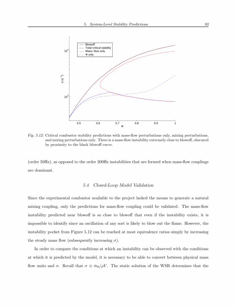
5. System-Level Stability Predictions 93
0.5 0.6 0.7 0.8 0.9 1
103
104
Φ
σ (s
−1 )
BlowoffTotal critical stabilityMass−flow onlyΦ only
Fig. 5.12: Critical combustor stability predictions with mass-flow perturbations only, mixing perturbations,and mixing perturbations only. There is a mass-flow instability extremely close to blowoff, obscuredby proximity to the black blowoff curve.
(order 50Hz), as opposed to the order 200Hz instabilities that are formed when mass-flow couplings
are dominant.
5.4 Closed-Loop Model Validation
Since the experimental combustor available to the project lacked the means to generate a natural
mixing coupling, only the predictions for mass-flow coupling could be validated. The mass-flow
instability predicted near blowoff is so close to blowoff that even if the instability exists, it is
impossible to identify since an oscillation of any sort is likely to blow out the flame. However, the
instability pocket from Figure 5.12 can be reached at most equivalence ratios simply by increasing
the steady mass flow (subsequently increasing σ).
In order to compare the conditions at which an instability can be observed with the conditions
at which it is predicted by the model, it is necessary to be able to convert between physical mass
flow units and σ. Recall that σ ≡ m0/ρV . The static solution of the WSR determines that the

5. System-Level Stability Predictions 94
density in the flame is on the order ρ ≈ 0.2 kgm3 . The flame can be optically measured to roughly on
the order V ≈ 10−3m3 in volume. So, for this particular experiment, the mass flow may crudely be
related to σ by
σ ≈ (5 × 10³kg−1)m0.
With this estimation, the lowest flow rate at which instability is predicted in Figure 5.12 is on the
order of 0.2kg/s, which was well above the capabilities of the experimental combustor. Therefore,
to the extent that no instability was observed in the operable conditions, the experiment failed to
contradict the model. It became apparent that if data were to be generated in support of the model
predictions, it would be necessary to modify the experiment.
Validation through Modified Combustor Acoustics
It is well understood that lengthening a combustor tends to encourage instabilities. In the light
of the above analysis, it becomes clear that doing so has the simultaneous affects of reducing the
resonant frequencies and increasing the open-loop gain, both of which encourage instability. In this
case, the objective was to increase the acoustic gain as to reduce the minimum gain in the flame
necessary for the induction of instability. To that end, a chimney was added to the combustor and
new acoustic transfer functions were produced using the procedure outlined in Chapter 4.
With the modification, at sufficiently high flow rates, the combustor exhibited an instability
well within sustainable operating conditions. Instability was experimentally identified by selecting
an air mass flow rate and gradually increasing fuel flow rate until a sustained tone was audible.
At most conditions the onset of instability introduced sufficiently violent acoustic oscillations as to
make identifying the instability trivial. At certain conditions, however, the onset of these violent
oscillations was preceded by a low-amplitude tone subtle enough to possibly be a lightly damped
resonance excited by flow noise rather than an actual instability. In these cases, the formal iden-
tification of instability was more difficult. Figure 5.13 shows individual data points that represent
recorded transitions between stability and instability overplotted against the curves predicted with
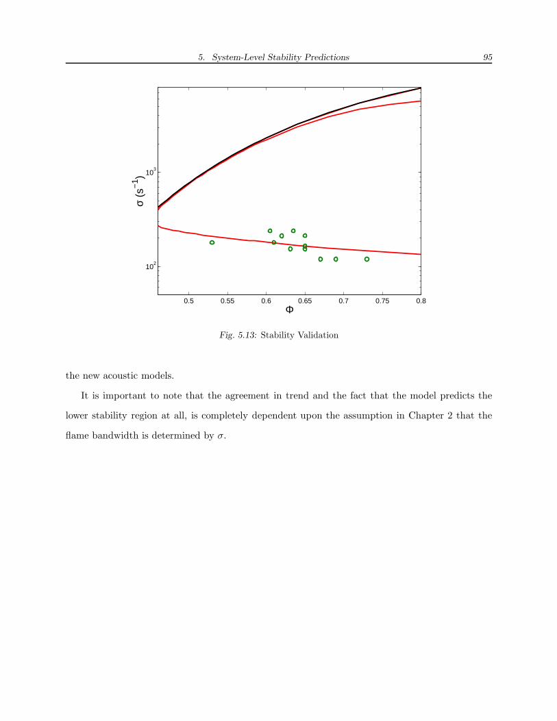
5. System-Level Stability Predictions 95
0.5 0.55 0.6 0.65 0.7 0.75 0.8
102
103
Φ
σ (s
−1 )
Fig. 5.13: Stability Validation
the new acoustic models.
It is important to note that the agreement in trend and the fact that the model predicts the
lower stability region at all, is completely dependent upon the assumption in Chapter 2 that the
flame bandwidth is determined by σ.
6. CONCLUSIONS
With Regards to the Flame
First and foremost among the implications of the work described herein is that the turbulent flame
exhibits a cutoff frequency corresponding to a time constant equal to the mean particle residence
time in the flame. Residence time may be expressed as it was in this work, τres = M/m0, or
as might be viewed as a more typical expression, τres = L/u, but certain important qualities are
consistent from realization to realization: that the residence time is a ratio between a measure of
flame size and fluid velocity. Consequently, accurately capturing dynamic changes in flame size is
paramount to the construction of an accurate dynamic flame model. Though these can be shown
not to influence the pole locations significantly if at all, such changes in flame size exhibit great
influence on the zeros and consequently the characteristics of the frequency response.
Well-Stirred Reactors are inherently under constrained to make to make the dynamic predictions
necessary to account for this fact. More specifically, the WSR is conceived such that the flame size
is an external constraint and the absence of spatial variations fundamental to the WSR eliminates
the potential to modify the model without some empirical knowledge or secondary flame size model
taking these effects into account.
With Regards to Turbulent Mixing
Linear, stochastic turbulent diffusion matches extremely well with experimental results, even in the
presence of certain complex geometries including area changes, swirlers, and center bodies. As a
result of the linear diffusion model,
Fcutoff σt = 0.13

6. Conclusions 97
is an excellent predictor of the mixing transfer function’s cutoff frequency for reasonable ratios of
U2/v2.
With Regards to the Stability of a Turbulent Premixed Combustor
The closed loop models indicate with limited experimental validation that velocity (mass flow)
perturbations are likely to influence combustion dynamics between two and four orders of magnitude
(40 to 80dB) more strongly than mixing perturbations. Since the flame and mixing DC gains are
determined mostly by geometry-independent parameters, unless combustor acoustics local to the
injection plane are engineered to exhibit unusually strong gains, the mixing perturbations described
herein are irrelevant to the occurrence of combustion instability.
It is evident in Figure 5.5 just how sensitive the stability bounds are to changes in the acoustic
transfer function. The mere addition of damping to existing peaks (much less the total removal
or addition of peaks) can drastically alter the characteristics of the stability map, even adding or
removing pockets of instability. This is not only due to the importance of the transfer function
magnitudes. Since the direct coupling between the flame and the acoustics does not involve any
significant delay, the only dynamics capable of causing the 360◦ phase crossings necessary for
instability are to be found in the acoustics.
For this reason, if combustor geometry is to be designed with its acoustic characteristics in
mind, the acoustic transfer function between the flame heat release rate and the velocity at the
dump plane should not have resonant peaks (pole pairs) that are not paired with resonant troughs
(zero pairs) at low frequencies. Consecutive resonant peaks result in exactly 360◦ of phase lag which
ensures a crossing. If crossings occur at low frequencies where the flame has a significant response,
then instability is likely.
Most importantly, the limited validation performed on the model seems to encourage the use
of system-level models to predict instabilities. The closed-loop model successfully made order
of magnitude and trend predictions for the occurrence of instability in the modified combustor
without any prior knowledge of the modified combustor’s stability characteristics. The results even
contradicted common knowledge regarding instabilities by occurring at higher equivalence ratios

6. Conclusions 98
rather than ultra-lean equivalence ratios, but were found to be accurate nonetheless.
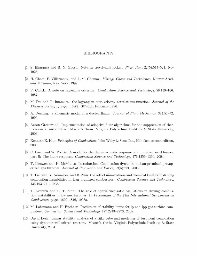
BIBLIOGRAPHY
[1] S. Bhargava and R. N. Ghosh. Note on trevelyan’s rocker. Phys. Rev., 22(5):517–521, Nov1923.
[2] H. Chate, E. Villermaux, and J.-M. Chomaz. Mixing: Chaos and Turbulence. Kluwer Acad-emic/Plenum, New York, 1999.
[3] F. Culick. A note on rayleigh’s criterion. Combustion Science and Technology, 56:159–166,1987.
[4] M. Doi and T. Imamura. the lagrangian auto-velocity correlations function. Journal of thePhysical Society of Japan, 55(2):507–511, February 1986.
[5] A. Dowling. a kinematic model of a ducted flame. Journal of Fluid Mechanics, 394:51–72,1999.
[6] Aaron Greenwood. Implementation of adaptive filter algorithms for the suppression of ther-moacoustic instabilities. Master’s thesis, Virginia Polytechnic Institute & State University,2003.
[7] Kenneth K. Kuo. Principles of Combustion. John Wiley & Sons, Inc., Hoboken, second edition,2005.
[8] C. Lawn and W. Polifke. A model for the thermoacoustic response of a premixed swirl burner,part ii: The flame response. Combustion Science and Technology, 176:1359–1390, 2004.
[9] T. Lieuwen and K. McManus. Introduction: Combustion dynamics in lean-premixed prevap-orized gas turbines. Journal of Propulsion and Power, 19(5):721, 2003.
[10] T. Lieuwen, Y. Neumeier, and B. Zinn. the role of unmixedness and chemical kinetics in drivingcombustion instabilities in lean premixed combustors. Combustion Science and Technology,135:193–211, 1998.
[11] T. Lieuwen and B. T. Zinn. The role of equivalence ratio oscillations in driving combus-tion instabilities in low nox turbines. In Proceedings of the 27th International Symposium onCombustion, pages 1809–1816, 1998a.
[12] M. Lohrmann and H. Buchner. Prediction of stability limits for lp and lpp gas turbine com-bustors. Combustion Science and Technology, 177:2243–2273, 2005.
[13] David Losh. Linear stability analysis of a rijke tube and modeling of turbulent combustionusing dynamic well-stirred reactors. Master’s thesis, Virginia Polytechnic Institute & StateUniversity, 2004.
Bibliography 100
[14] Rajendran Mohanraj, Yedidia Neumeier, and Ben Zinn. Combustor model for simulation ofcombustion instabilities and their active control. Journal of Propulsion and Power, 16(3):485–491, 2000.
[15] Ali Hasan Nayfeh. Introduction to Perturbation Techniques. John Wiley & Sons, New York,first edition, 1981.
[16] Lars Nord. A thermoacoustic characterization of a rijke-type tube combustor. Master’s thesis,Virginia Polytechnic Institute & State University, 2001.
[17] Ronald L. Panton. Incompressible Flow. John Wiley & Sons, Inc., New York, 1996.
[18] S. Park, A. Annasway, and A. Ghoniem. Heat release dynamics modeling of kinetically con-trolled burning. Combustion and Flame, 128:217–231, 2002.
[19] Preetham and T. Lieuwen. Nonlinear flame-flow transfer function calculations: Flow distur-bance celerity effects. In 40th AIAA/ASME/SAE/ASEE Joint Propulsion Conference andExhibit, 2004.
[20] Preetham and T. Lieuwen. Nonlinear flame-flow transfer function calculations: Flow distur-bance celerity effects part 2. In 43rd AIAA/ASME/SAE/ASEE Joint Propulsion Conferenceand Exhibit, 2004.
[21] A. Putnam and W. Dennis. Survey of organ-pipe oscillations in combustion systems. AcousticalSociety of America, 28(2), 1956.
[22] Abbott A. Putnam. Combustion-Driven Oscillations in Industry. American Elsevier Pub. Co.,New York, 1971.
[23] J. Rayleigh. The Theory of Sound. Dover Publications, New York, second edition, 1945.
[24] T. Scarinci and C. Freeman. the propogation of a fuel-air ratio disturbance in a simple premixerand its influence on pressure wave amplification. In Proceedings of the ASME Turbo Exo 2000,volume 2000-GT-0106, 2000.
[25] Stephen R. Turns. An Introduction to Combustion. McGraw Hill, New York, second edition,2000.
[26] J. Tyndal. Sound. D. Appleton & Co., New York, 1897.