Embed Size (px)
Citation preview

2
System Reliability Concepts
The analysis of the reliability of a system must be based on precisely defined concepts. Since it is readily accepted that a population of supposedly identical systems, operating under similar conditions, fall at different points in time, then a failure phenomenon can only be described in probabilistic terms. Thus, the fundamental definitions of reliability must depend on concepts from probability theory. This chapter describes the concepts of system reliability engineering. These concepts provide the basis for quantifying the reliability of a system. They allow precise comparisons between systems or provide a logical basis for improvement in a failure rate. Various examples reinforce the definitions as presented in Section 2.1. Section 2.2 examines common distribution functions useful in reliability engineering. Several distribution models are discussed and the resulting hazard functions are derived. Section 2.3 describes a new concept of systemability. Several systemability functions of various system configurations such as series, parallel, and k-out-of-n, are presented. Section 2.4 discusses various reliability aspects of systems with multiple failure modes. Stochastic processes including Markov process, Poisson process, renewal process, quasi-renewal process, and nonhomogeneous Poisson process are discussed in Sections 2.5 and 2.6.
In general, a system may be required to perform various functions, each of which may have a different reliability. In addition, at different times, the system may have a different probability of successfully performing the required function under stated conditions. The term failure means that the system is not capable of performing a function when required. The term capable used here is to define if the system is capable of performing the required function. However, the term capable is unclear and only various degrees of capability can be defined.

10 System Software Reliability
2.1 Reliability Measures
The reliability definitions given in the literature vary between different practition- ers as well as researchers. The generally accepted definition is as follows. Definition 2.1: Reliability is the probability of success or the probability that the system will perform its intended function under specified design limits.
More specific, reliability is the probability that a product or part will operate properly for a specified period of time (design life) under the design operating conditions (such as temperature, volt, etc.) without failure. In other words, reliability may be used as a measure of the system’s success in providing its function properly. Reliability is one of the quality characteristics that consumers require from the manufacturer of products. Mathematically, reliability R(t) is the probability that a system will be successful in the interval from time 0 to time t:
( ) ( ) 0= > ≥R t P T t t (2.1)
where T is a random variable denoting the time-to-failure or failure time. Unreliability F(t), a measure of failure, is defined as the probability that the sys-tem will fail by time t:
( ) ( ) for 0= ≤ ≥F t P T t t
In other words, F(t) is the failure distribution function. If the time-to-failure random variable T has a density function f(t), then
( ) ( )∞
= ∫t
R t f s ds
or, equivalently,
( ) [ ( )]= − df t R t
dt
The density function can be mathematically described in terms of T:
0
lim ( )Δ →
< ≤ + Δt
P t T t t
This can be interpreted as the probability that the failure time T will occur between the operating time t and the next interval of operation, t+Δt.
Consider a new and successfully tested system that operates well when put into service at time t = 0. The system becomes less likely to remain successful as the time interval increases. The probability of success for an infinite time interval, of course, is zero.
Thus, the system functions at a probability of one and eventually decreases to a probability of zero. Clearly, reliability is a function of mission time. For example, one can say that the reliability of the system is 0.995 for a mission time of 24 hours. However, a statement such as the reliability of the system is 0.995 is meaningless because the time interval is unknown.

System Reliability Concepts 11
Example 2.1: A computer system has an exponential failure time density function
9,0001( ) 0
9,000
−= ≥
t
f t e t
What is the probability that the system will fail after the warranty (six months or 4380 hours) and before the end of the first year (one year or 8760 hours)? Solution: From equation (2.1) we obtain
8760
9000
4380
1(4380 8760)
9000
0.237
−< ≤ =
=
∫t
P T e dt
This indicates that the probability of failure during the interval from six months to one year is 23.7%.
If the time to failure is described by an exponential failure time density function, then
1
( ) 0, 0θ θθ
−= ≥ >
t
f t e t (2.2)
and this will lead to the reliability function
1
( ) 0θ θ
θ
∞− −
= = ≥∫s t
t
R t e ds e t (2.3)
Consider the Weibull distribution where the failure time density function is given by
1
( ) 0, 0, 0
β
βθ
ββ θ βθ
⎛ ⎞⎜− − ⎟⎜ ⎠⎝= ≥ > >t
tf t e t
Then the reliability function is
( ) 0
β
θ⎛ ⎞⎜− ⎟⎜ ⎠⎝= ≥
t
R t e t
Thus, given a particular failure time density function or failure time distribution function, the reliability function can be obtained directly. Section 2.2 provides further insight for specific distributions. System Mean Time to Failure Suppose that the reliability function for a system is given by R(t). The expected failure time during which a component is expected to perform successfully, or the system mean time to failure (MTTF), is given by
0
( )∞
= ∫MTTF t f t dt (2.4)
Substituting
( ) [ ( )]= − df t R t
dt
into equation (2.4) and performing integration by parts, we obtain

12 System Software Reliability
0
00
[ ( )]
[ ( )] | ( )
MTTF td R t
tR t R t dt
∞
∞∞
= −
= − +
∫
∫ (2.5)
The first term on the right-hand side of equation (2.5) equals zero at both limits, since the system must fail after a finite amount of operating time. Therefore, we must have tR(t) → 0 as t → ∞ . This leaves the second term, which equals
0
( )∞
= ∫MTTF R t dt (2.6)
Thus, MTTF is the definite integral evaluation of the reliability function. In general, if ( )λ t is defined as the failure rate function, then, by definition, MTTF is not equal to 1/ ( )λ t .
The MTTF should be used when the failure time distribution function is specified because the reliability level implied by the MTTF depends on the underlying failure time distribution. Although the MTTF measure is one of the most widely used reliability calculations, it is also one of the most misused calculations. It has been misinterpreted as “guaranteed minimum lifetime”. Consider the results as given in Table 2.1 for a twelve-component life duration test.
Table 2.1. Results of a twelve-component life duration test
Component Time to failure (hours)
1 2 3 4 5 6 7 8 9
10 11 12
4510 3690 3550 5280 2595 3690 920 3890 4320 4770 3955 2750
Using a basic averaging technique, the component MTTF of 3660 hours was
estimated. However, one of the components failed after 920 hours. Therefore, it is important to note that the system MTTF denotes the average time to failure. It is neither the failure time that could be expected 50% of the time, nor is it the guaran-teed minimum time of system failure.
A careful examination of equation (2.6) will show that two failure distributions can have the same MTTF and yet produce different reliability levels. This is illustrated in a case where the MTTFs are equal, but with normal and exponential

System Reliability Concepts 13
failure distributions. The normal failure distribution is symmetrical about its mean, thus ( ) ( 0) 0.5= ≥ =R MTTF P Z
where Z is a standard normal random variable. When we compute for the exponential failure distribution using equation (2.3), recognizing that θ = MTTF, the reliability at the MTTF is
( ) 0.368−
= =MTTF
MTTFR MTTF e
Clearly, the reliability in the case of the exponential distribution is about 74% of that for the normal failure distribution with the same MTTF. Failure Rate Function The probability of a system failure in a given time interval [t1, t2] can be expressed in terms of the reliability function as
2
1 1 2
1 2
( ) ( ) ( )
( ) ( )
∞ ∞
= −
= −
∫ ∫ ∫t
t t t
f t dt f t dt f t dt
R t R t
or in terms of the failure distribution function (or the unreliability function) as
2 2 1
1
2 1
( ) ( ) ( )
( ) ( )
−∞ −∞
= −
= −
∫ ∫ ∫t t t
t
f t dt f t dt f t dt
F t F t
The rate at which failures occur in a certain time interval [t1, t2] is called the failure rate. It is defined as the probability that a failure per unit time occurs in the interval, given that a failure has not occurred prior to t1, the beginning of the interval. Thus, the failure rate is
1 2
2 1 1
( ) ( )
( ) ( )
−−
R t R t
t t R t
Note that the failure rate is a function of time. If we redefine the interval as [ , ],+ Δt t t the above expression becomes
( ) ( )
( )
− + ΔΔ
R t R t t
tR t
The rate in the above definitions is expressed as failures per unit time, when in reality, the time units might be in terms of miles, hours, etc. The hazard function is defined as the limit of the failure rate as the interval approaches zero. Thus, the hazard function h(t) is the instantaneous failure rate, and is defined by
0
( ) ( )( ) lim
( )
1 [ ( )]
( )
( )
( )
Δ →
− + Δ=Δ
= −
=
t
R t R t th t
tR t
dR t
R t dt
f t
R t
(2.7)

14 System Software Reliability
The quantity h(t)dt represents the probability that a device of age t will fail in the small interval of time t to (t+dt). The importance of the hazard function is that it indicates the change in the failure rate over the life of a population of components by plotting their hazard functions on a single axis. For example, two designs may provide the same reliability at a specific point in time, but the failure rates up to this point in time can differ.
The death rate, in statistical theory, is analogous to the failure rate as the force of mortality is analogous to the hazard function. Therefore, the hazard function or hazard rate or failure rate function is the ratio of the probability density function (pdf) to the reliability function. Maintainability When a system fails to perform satisfactorily, repair is normally carried out to locate and correct the fault. The system is restored to operational effectiveness by making an adjustment or by replacing a component.
Maintainability is defined as the probability that a failed system will be restored to specified conditions within a given period of time when maintenance is performed according to prescribed procedures and resources. In other words, maintainability is the probability of isolating and repairing a fault in a system within a given time. Maintainability engineers must work with system designers to ensure that the system product can be maintained by the customer efficiently and cost effectively. This function requires the analysis of part removal, replacement, tear-down, and build-up of the product in order to determine the required time to carry out the operation, the necessary skill, the type of support equipment and the documentation.
Let T denote the random variable of the time to repair or the total downtime. If the repair time T has a repair time density function g(t), then the maintainability, V(t), is defined as the probability that the failed system will be back in service by time t, i.e.,
0
( ) ( ) ( )= ≤ = ∫t
V t P T t g s ds
For example, if ( ) μμ −= tg t e where μ > 0 is a constant repair rate, then
( ) 1 μ−= − tV t e
which represents the exponential form of the maintainability function. An important measure often used in maintenance studies is the mean time to
repair (MTTR) or the mean downtime. MTTR is the expected value of the random variable repair time, not failure time, and is given by
0
( )∞
= ∫MTTR tg t dt
When the distribution has a repair time density given by ( ) μμ −= tg t e , then, from the above equation, MTTR = 1/ μ . When the repair time T has the log normal density function g(t), and the density function is given by

System Reliability Concepts 15
2
2
(ln )
21
( ) 02
μσ
π σ
−−= >
t
g t e tt
then it can be shown that
2
2
σ
=MTTR m e
where m denotes the median of the log normal distribution. In order to design and manufacture a maintainable system, it is necessary to
predict the MTTR for various fault conditions that could occur in the system. This is generally based on past experiences of designers and the expertise available to handle repair work.
The system repair time consists of two separate intervals: passive repair time and active repair time. Passive repair time is mainly determined by the time taken by service engineers to travel to the customer site. In many cases, the cost of travel time exceeds the cost of the actual repair. Active repair time is directly affected by the system design and is listed as follows:
1. The time between the occurrence of a failure and the system user becoming aware that it has occurred.
2. The time needed to detect a fault and isolate the replaceable component(s).
3. The time needed to replace the faulty component(s). 4. The time needed to verify that the fault has been corrected and the system
is fully operational. The active repair time can be improved significantly by designing the system in such a way that faults may be quickly detected and isolated. As more complex systems are designed, it becomes more difficult to isolate the faults. Availability Reliability is a measure that requires system success for an entire mission time. No failures or repairs are allowed. Space missions and aircraft flights are examples of systems where failures or repairs are not allowed. Availability is a measure that allows for a system to repair when failure occurs.
The availability of a system is defined as the probability that the system is successful at time t. Mathematically,
System up timeAvailability =
System up time + System down time
MTTF =
MTTF + MTTR
Availability is a measure of success used primarily for repairable systems. For non-repairable systems, availability, A(t), equals reliability, R(t). In repairable systems, A(t) will be equal to or greater than R(t).
The mean time between failures (MTBF) is an important measure in repairable systems. This implies that the system has failed and has been repaired. Like MTTF

16 System Software Reliability
and MTTR, MTBF is an expected value of the random variable time between failures. Mathematically, MTBF = MTTF + MTTR
The term MTBF has been widely misused. In practice, MTTR is much smaller than MTTF, which is approximately equal to MTBF. MTBF is often incorrectly substituted for MTTF, which applies to both repairable systems and non-repairable systems. If the MTTR can be reduced, availability will increase, and the system will be more economical.
A system where faults are rapidly diagnosed is more desirable than a system that has a lower failure rate but where the cause of a failure takes longer to detect, resulting in a lengthy system downtime. When the system being tested is renewed through maintenance and repairs, E(T) is also known as MTBF.
2.2 Common Distribution Functions
This section presents some of the common distribution functions and several hazard models that have applications in reliability engineering (Pham 2000a). Binomial Distribution The binomial distribution is one of the most widely used discrete random variable distributions in reliability and quality inspection. It has applications in reliability engineering, e.g., when one is dealing with a situation in which an event is either a success or a failure.
The pdf of the distribution is given by
( )
( )( ) (1 ) 0, 1, 2, ...,
!
!( )!
−= = − =
=−
x n xnP X x p p x nx
nnx x n x
where n = number of trials; x = number of successes; p = single trial probability of success.
The reliability function, R(k), (i.e., at least k out of n items are good) is given by
( )( ) (1 ) −
=
= −∑n
x n x
x k
nR k p px
Example 2.2: Suppose in the production of lightbulbs, 90% are good. In a random sample of 20 lightbulbs, what is the probability of obtaining at least 18 good lightbulbs? Solution: The probability of obtaining 18 or more good lightbulbs in the sample of 20 is

System Reliability Concepts 17
2020
18
20(18) (0.9) (0.1)
18
0.667
x x
x
R −
=
⎛ ⎞= ⎜ ⎟
⎝ ⎠
=
∑
Poisson Distribution Although the Poisson distribution can be used in a manner similar to the binomial distribution, it is used to deal with events in which the sample size is unknown. This is also a discrete random variable distribution whose pdf is given by
( )( ) for 0, 1, 2, ....
!
x tt eP X x x
x
λλ −
= = =
where λ = constant failure rate, x = is the number of events. In other words, P(X = x) is the probability of exactly x failures occurring in time t. Therefore, the reliability Poisson distribution, R(k) (the probability of k or fewer failures) is given by
0
( )( )
!
λλ −
=
=∑x tk
x
t eR k
x
This distribution can be used to determine the number of spares required for the reliability of standby redundant systems during a given mission. Exponential Distribution Exponential distribution plays an essential role in reliability engineering because it has a constant failure rate. This distribution has been used to model the lifetime of electronic and electrical components and systems. This distribution is appropriate when a used component that has not failed is as good as a new component - a rather restrictive assumption. Therefore, it must be used diplomatically since numerous applications exist where the restriction of the memoryless property may not apply. For this distribution, we have reproduced equations (2.2) and (2.3), respectively:
1
( ) , 0
( ) , 0
λθ
λθ
λθ
− −
− −
= = ≥
= = ≥
tt
tt
f t e e t
R t e e t
where θ = 1/λ > 0 is an MTTF’s parameter and λ ≥ 0 is a constant failure rate. The hazard function or failure rate for the exponential density function is
constant, i.e.,
11
( ) 1( )
1( )
θθ λ
θθ
−
= = = =−
ef t
h tR t
e
The failure rate for this distribution is λ, a constant, which is the main reason for this widely used distribution. Because of its constant failure rate property, the exponential is an excellent model for the long flat “intrinsic failure” portion of the
18 System Software Reliability
bathtub curve. Since most parts and systems spend most of their lifetimes in this portion of the bathtub curve, this justifies frequent use of the exponential (when early failures or wear out is not a concern). The exponential model works well for inter-arrival times. When these events trigger failures, the exponential lifetime model can be used.
We will now discuss some properties of the exponential distribution that are useful in understanding its characteristics, when and where it can be applied. Property 2.1: (Memoryless property) The exponential distribution is the only continuous distribution satisfying
{ } { | } for 0, 0≥ = ≥ + ≥ > >P T t P T t s T s t s (2.8)
This result indicates that the conditional reliability function for the lifetime of a component that has survived to time s is identical to that of a new component. This term is the so-called "used-as-good-as-new" assumption.
The lifetime of a fuse in an electrical distribution system may be assumed to have an exponential distribution. It will fail when there is a power surge causing the fuse to burn out. Assuming that the fuse does not undergo any degradation over time and that power surges that cause failure are likely to occur equally over time, then use of the exponential lifetime distribution is appropriate, and a used fuse that has not failed is as good as new. Property 2.2: If T1, T2, ..., Tn, are independently and identically distributed exponential random variables (RVs) with a constant failure rate λ, then
2
1
2 ~ (2 )λ χ=∑
n
ii
T n
where 2 (2 )χ n is a chi-squared distribution with degrees of freedom 2n. This result
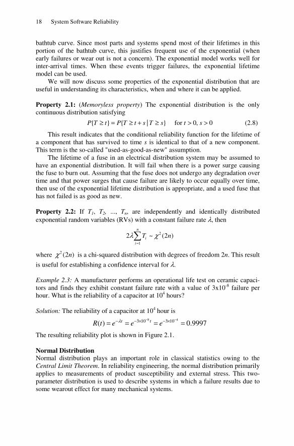
is useful for establishing a confidence interval for λ. Example 2.3: A manufacturer performs an operational life test on ceramic capaci-tors and finds they exhibit constant failure rate with a value of 3x10⁻⁸ failure per hour. What is the reliability of a capacitor at 104 hours? Solution: The reliability of a capacitor at 104 hour is
8 43 10 3 10( ) 0.9997λ − −− − × − ×= = = =t tR t e e e
The resulting reliability plot is shown in Figure 2.1. Normal Distribution Normal distribution plays an important role in classical statistics owing to the Central Limit Theorem. In reliability engineering, the normal distribution primarily applies to measurements of product susceptibility and external stress. This two- parameter distribution is used to describe systems in which a failure results due to some wearout effect for many mechanical systems.

System Reliability Concepts 19
0.6
0.7
0.8
0.9
1
0 2000000 4000000 6000000 8000000 10000000
Figure 2.1. Reliability function vs time
The normal distribution takes the well-known bell shape. This distribution is symmetrical about the mean and the spread is measured by variance. The larger the value, the flatter the distribution. The pdf is given by
21
( )21
( ) -2
μσ
σ π
−−= ∞ < < ∞
t
f t e t
where μ is the mean value and σ is the standard deviation. The cumulative distri- bution function (cdf) is
21
( )21
( )2
t s
F t e dsμ
σ
σ π
−−
−∞
= ∫
The reliability function is
21
( )21
( )2
s
t
R t e dsμ
σ
σ π
∞ −−= ∫
There is no closed form solution for the above equation. However, tables for the standard normal density function are readily available (see Table A1.1 in Appendix 1) and can be used to find probabilities for any normal distribution. If
μ
σ−= T
Z
is substituted into the normal pdf, we obtain
2
21
( ) -2π
−= ∞ < < ∞
z
f z e Z
This is a so-called standard normal pdf, with a mean value of 0 and a standard deviation of 1. The standardized cdf is given by
21
21( )
2π−
−∞
Φ = ∫t
st e ds (2.9)

20 System Software Reliability
where Φ is a standard normal distribution function. Thus, for a normal random variable T, with mean μ and standard deviation σ,
( )μ μ
σ σ− −⎛ ⎞ ⎛ ⎞≤ = ≤ = Φ⎜ ⎟ ⎜ ⎟
⎝ ⎠ ⎝ ⎠
t tP T t P Z
where Φ yields the relationship necessary if standard normal tables are to be used. The hazard function for a normal distribution is a monotonically increasing function of t. This can be easily shown by proving that h’(t) ≥ 0 for all t. Since
( )
( )( )
= f th t
R t
then (see Problem 15)
2
2
( ) '( ) ( )'( ) 0
( )
+= ≥R t f t f th t
R t (2.10)
One can try this proof by employing the basic definition of a normal density function f. Example 2.4: A component has a normal distribution of failure times with μ = 2000 hours and σ = 100 hours. Find the reliability of the component and the hazard function at 1900 hours. Solution: The reliability function is related to the standard normal deviate z by
( )μ
σ−⎛ ⎞= >⎜ ⎟
⎝ ⎠
tR t P Z
where the distribution function for Z is given by equation (2.9). For this particular application,
( )
1900 2000(1900)
100
1
−⎛ ⎞= >⎜ ⎟⎝ ⎠
= > −
R P Z
P z
From the standard normal table in Table A1.1 in Appendix 1, we obtain (1900) 1 ( 1) 0.8413.= − Φ − =R
The value of the hazard function is found from the relationship
( )
( )( ) ( )
μσ
σ
−⎛ ⎞Φ =⎜ ⎟⎝ ⎠= =
tz
f th t
R t R t
where φ is a pdf of standard normal density. Here
( 1.0) 0.1587(1900)
( ) 100(0.8413)
0.0019 failures/cycle
σΦ −= =
=
hR t
Example 2.5: A part has a normal distribution of failure times with μ = 40000 cycles and σ = 2000 cycles. Find the reliability of the part at 38000 cycles.

System Reliability Concepts 21
Solution: The reliability at 38000 cycles
38000 40000(38000)
2000
( 1.0)
(1.0) 0.8413
−⎛ ⎞= >⎜ ⎟⎝ ⎠
= > −= Φ =
R P z
P z
The resulting reliability plot is shown in Figure 2.2. The normal distribution is flexible enough to make it a very useful empirical model. It can be theoretically derived under assumptions matching many failure mechanisms. Some of these are corrosion, migration, crack growth, and in general, failures resulting from chemical reactions or processes. That does not mean that the normal is always the correct model for these mechanisms, but it does perhaps explain why it has been empirically successful in so many of these cases. Log Normal Distribution The log normal lifetime distribution is a very flexible model that can empirically fit many types of failure data. This distribution, with its applications in maintainability engineering, is able to model failure probabilities of repairable systems and to model the uncertainty in failure rate information. The log normal density function is given by
21 ln
21( ) 0
2
μσ
σ π
−⎛ ⎞− ⎜ ⎟⎝ ⎠= ≥
t
f t e tt
(2.11)
where μ and σ are parameters such that -∞ < μ < ∞, and σ > 0. Note that μ and σ are not the mean and standard deviations of the distribution.
Reliability Curve
00,10,20,30,40,50,60,70,80,9
1
35000 37000 39000 41000 43000 45000 47000 49000 51000 53000
Figure 2.2. Normal reliability plot vs time

22 System Software Reliability
The relationship to the normal (just take natural logarithms of all the data and time points and you have “normal” data) makes it easy to work with many good software analysis programs available to treat normal data.
Mathematically, if a random variable X is defined as X = lnT, then X is normally distributed with a mean of μ and a variance of σ 2. That is,
E(X) = E(lnT) = μ and
V(X) = V(lnT) = σ 2. Since T = eX, the mean of the log normal distribution can be found by using the
normal distribution. Consider that
21
21
( ) ( )2
μσ
σ π
⎡ ⎤−⎛ ⎞∞ −⎢ ⎥⎜ ⎟⎝ ⎠⎢ ⎥⎣ ⎦
−∞
= = ∫x
xXE T E e e dx
and by rearrangement of the exponent, this integral becomes
22 2
2
1[ ( )]
221
( )2
σ μ σμσ
σ π
∞ − − ++
−∞
= ∫x
E T e e dx
Thus, the mean of the log normal distribution is
2
2( )σμ +
=E T e
Proceeding in a similar manner,
22 2 2( )( ) ( ) μ σ+= =XE T E e e
thus, the variance for the log normal is
2 22( ) ( 1)μ σ σ+= −V T e e
The cumulative distribution function for the log normal is
21 ln
( )2
0
1( )
2
μσ
σ π
−−= ∫
t s
F t e dss
and this can be related to the standard normal deviate Z by
( ) [ ] (ln ln )
ln
μσ
= ≤ = ≤
− ⎤⎡= ≤ ⎥⎢⎣ ⎦
F t P T t P T t
tP Z
Therefore, the reliability function is given by
ln
( )μ
σ− ⎤⎡= > ⎥⎢⎣ ⎦
tR t P Z (2.12)
and the hazard function would be
( )ln
( )( )
( ) ( )
μσ
σ
−Φ= =
tf t
h tR t t R t
where Φ is a cdf of standard normal density.

System Reliability Concepts 23
Example 2.6: The failure time of a certain component is log normal distributed with μ = 5 and σ = 1. Find the reliability of the component and the hazard rate for a life of 50 time units. Solution: Substituting the numerical values of μ, σ, and t into equation (2.12), we compute
ln 50 5
(50) [ 1.09]1
0.8621
− ⎤⎡= > = > −⎥⎢⎣ ⎦=
R P Z P Z
Similarly, the hazard function is given by
( )ln 50 5
1(50) 0.032 failures/unit.50(1)(0.8621)
−Φ= =h
Thus, values for the log normal distribution are easily computed by using the standard normal tables. Example 2.7: The failure time of a part is log normal distributed with μ = 6 and σ = 2. Find the part reliability for a life of 200 time units. Solution: The reliability for the part of 200 time units is
ln 200 6
(200) ( 0.35)2
0.6368
−⎛ ⎞= > = > −⎜ ⎟⎝ ⎠
=
R P Z P Z
Reliability Curve
00.10.20.30.40.50.60.70.80.9
1
0 1000 2000 3000 4000 5000
Figure 2.3. Log normal reliability plot vs time
The log normal lifetime model, like the normal, is flexible enough to make it a very useful empirical model. Figure 2.3 shows the reliability of the log normal vs time. It can be theoretically derived under assumptions matching many failure

24 System Software Reliability
mechanisms. Some of these are: corrosion and crack growth, and in general, failures resulting from chemical reactions or processes.
Weibull Distribution The exponential distribution is often limited in applicability owing to the memoryless property. The Weibull distribution (Weibull 1951) is a generalization of the exponential distribution and is commonly used to represent fatigue life, ball bearing life, and vacuum tube life. The Weibull distribution is extremely flexible and appropriate for modeling component lifetimes with fluctuating hazard rate functions and for representing various types of engineering applications. The three-parameters probability density function is
1( )
( ) 0
βγβθ
ββ γ γ
θ
−⎛ ⎞− −⎜ ⎟⎝ ⎠−= ≥ ≥
tt
f t e t
where θ and β are known as the scale and shape parameters, respectively, and γ
is known as the location parameter. These parameters are always positive. By using different parameters, this distribution can follow the exponential distribution, the normal distribution, etc. It is clear that, for t ≥ γ, the reliability function R(t) is
( ) for 0, 0, 0
βγθ γ β θ−⎛ ⎞−⎜ ⎟
⎝ ⎠= > > > >t
R t e t (2.13)
hence,
1( )
( ) 0, 0, 0β
ββ γ γ β θ
θ
−−= > > > >th t t (2.14)
It can be shown that the hazard function is decreasing for β < 1, increasing for β > 1, and constant when β = 1. Example 2.8: The failure time of a certain component has a Weibull distribution with β = 4, θ = 2000, and γ = 1000. Find the reliability of the component and the hazard rate for an operating time of 1500 hours. Solution: A direct substitution into equation (2.13) yields
41500 1000
2000(1500) 0.996−⎛ ⎞
⎜ ⎟⎝ ⎠
−= =R e
Using equation (2.14), the desired hazard function is given by 4 1
4
-5
4(1500 1000)(1500)
(2000)
3.13 x 10 failures/hour
h−−=
=
Note that the Rayleigh and exponential distributions are special cases of the Weibull distribution at β = 2, γ = 0, and β = 1, γ = 0, respectively. For example, when β = 1 and γ = 0, the reliability of the Weibull distribution function in equation (2.13) reduces to
( ) θ−
=t
R t e

System Reliability Concepts 25
and the hazard function given in equation (2.14) reduces to 1/θ, a constant. Thus, the exponential is a special case of the Weibull distribution. Similarly, when γ = 0 and β = 2, the Weibull probability density function becomes the Rayleigh density function. That is
2
2( ) for 0, 0θ θ
θ−
= > ≥t
f t te t
Other Forms of Weibull Distributions The Weibull distribution again is widely used in engineering applications. It was originally proposed for representing the distribution of the breaking strength of materials. The Weibull model is very flexible and also has theoretical justification in many applications as a purely empirical model. Another form of Weibull probability density function is, for example,
1( ) γγ λλ γ − −= tf x x e (2.15)
When γ=2, the density function becomes a Rayleigh distribution. It can easily be shown that the mean, variance and reliability of the above
Weibull distribution are, respectively, as follows:
Mean = 1
1(1 )γλ
γΓ +
Variance = 22
2 11 1γλ
γ γ
⎛ ⎞⎛ ⎞⎛ ⎞ ⎛ ⎞⎜ ⎟Γ + − Γ +⎜ ⎟⎜ ⎟ ⎜ ⎟⎜ ⎟⎝ ⎠ ⎝ ⎠⎝ ⎠⎝ ⎠ (2.16)
Reliability = γλ− te
Example 2.9: The time to failure of a part has a Weibull distribution with 1
λ=250
(measured in 105 cycles ) and γ=2. Find the part reliability at 106 cycles. Solution: The part reliability at 106 cycles is
26 (10) / 250(10 ) 0.6703−= =R e
The resulting reliability function is shown in Figure 2.4.

26 System Software Reliability
0 1 0 2 0 3 0 4 0 5 0 6 0 7 0 8 0 9 0 1 0 00
0 . 1
0 . 2
0 . 3
0 . 4
0 . 5
0 . 6
0 . 7
0 . 8
0 . 9
1W e ib u l l R e l ia b i l i t y C u rve
Figure 2.4. Weibull reliability function vs time
Gamma Distribution Gamma distribution can be used as a failure probability function for components whose distribution is skewed. The failure density function for a gamma distribution is
1
( ) 0, , 0( )
αβ
α α ββ α
− −= ≥ >
Γ
tt
f t e t (2.17)
where α is the shape parameter and β is the scale parameter. Hence,
11( )
( )α β
αβ α
∞ −−=
Γ∫s
t
R t s e ds
If α is an integer, it can be shown by successive integration by parts that
1
0
( ) ( )
!
αββ
−−
== ∑
it t
i
R t ei
(2.18)
and
11( )
1
0
( )( )
( )
( )
!
βα
β
αβ α
αβ
−−Γ
−−
=
= =
∑
t
tit
i
f th t
R t
t e
ei
The gamma density function has shapes that are very similar to the Weibull distribution. At α = 1, the gamma distribution becomes the exponential distribu- tion with the constant failure rate 1/β. The gamma distribution can also be used to model the time to the nth failure of a system if the underlying failure distribution is exponential. Thus, if Xi is exponentially distributed with parameter θ = 1/β, then T = X1 + X2 +…+Xn, is gamma distributed with parameters β and n.

System Reliability Concepts 27
Example 2.10: The time to failure of a component has a gamma distribution with α = 3 and β = 5. Determine the reliability of the component and the hazard rate at 10 time-units. Solution: Using equation (2.18), we compute
( )10 102
55
0(10) 0.6767
!
i
iR e
i
−
== =∑
From equation (2.17), we obtain
(10) 0.054
(10) 0.798 failures/unit time(10) 0.6767
= = =fh
R
The other form of the gamma probability density function can be written as follows:
1
( ) for >0( )
ttf x e t
α αββ
α
−−=
Γ (2.19)
This pdf is characterized by two parameters: shape parameter α and scale parameter β. When 0<α<1, the failure rate monotonically decreases; when α>1, the failure rate monotonically increase; when α=1 the failure rate is constant.
The mean, variance and reliability of the density function in equation (2.19) are, respectively,
Mean( MTTF) = αβ
Variance = 2
αβ
Reliability = 1
( )x
t
xe dx
α αββ
α
−∞ −
Γ∫
Example 2.11: A mechanical system time to failure is gamma distribution with α=3 and 1/β=120. Find the system reliability at 280 hours.
Solution: The system reliability at 280 hours is given by
2
280 2120
0
280120
(280) 0.85119!k
R ek
−
=
⎛ ⎞⎜ ⎟⎝ ⎠= =∑
and the resulting reliability plot is shown in Figure 2.5. The gamma model is a flexible lifetime model that may offer a good fit to
some sets of failure data. It is not, however, widely used as a lifetime distribution model for common failure mechanisms. A common use of the gamma lifetime model occurs in Bayesian reliability applications.

28 System Software Reliability
0 200 400 600 800 1000 1200 1400 1600 1800 20000
0.1
0.2
0.3
0.4
0.5
0.6
0.7
0.8
0.9
1Reliability for Gamma Distribution
Figure 2.5. Gamma reliability function vs time
Beta Distribution The two-parameter Beta density function, f(t), is given by
( )
( ) (1 ) 0 1, 0, 0( ) ( )
α βα β α βα β
Γ += − < < > >Γ Γ
f t t t t
where α and β are the distribution parameters. This two-parameter distribution is commonly used in many reliability engineering applications. Pareto Distribution The Pareto distribution was originally developed to model income in a population. Phenomena such as city population size, stock price fluctuations, and personal incomes have distributions with very long right tails. The probability density function of the Pareto distribution is given by
1
( )α
αα
+= kf t
t ≤ ≤ ∞k t
The mean, variance and reliability of the Pareto distribution are, respectively, Mean = /( 1) for 1α α− >k
Variance = 2
2 for 2
( 1) ( 2)
α αα α
>− −
K
Reliability = α
⎛ ⎞⎜ ⎟⎝ ⎠
k
t
The Pareto and log normal distributions have been commonly used to model the population size and economical incomes. The Pareto is used to fit the tail of the distribution, and the log normal is used to fit the rest of the distribution.

System Reliability Concepts 29
Rayleigh Distribution The Rayleigh function is a flexible lifetime distribution that can apply to many degra- dation process failure modes. The Rayleigh probability density function is
2
22
2( ) σ
σ
⎛ ⎞−⎜ ⎟⎜ ⎟⎝ ⎠=
tt
f t e (2.20)
The mean, variance, and reliability of Rayleigh function are, respectively,
Mean =
1
2
2
πσ ⎛ ⎞⎜ ⎟⎝ ⎠
Variance = 222
π σ⎛ ⎞−⎜ ⎟⎝ ⎠
Reliability =
2
2σ− t
e Example 2.12: Rolling resistance is a measure of the energy lost by a tire under load when it resists the force opposing its direction of travel. In a typical car, traveling at 60 miles per hour, about 20% of the engine power is used to overcome the rolling resistance of the tires.
A tire manufacturer introduces a new material that, when added to the tire rubber compound, significantly improves the tire rolling resistance but increases the wear rate of the tire tread. Analysis of a laboratory test of 150 tires shows that the failure rate of the new tire linearly increases with time (hours). It is expressed as
8( ) 0.5 10−= ×h t t
Find the reliability of the tire at one year.
Solution: The reliability of the tire after one year (8760 hours) of use is
8 20.5
10 (8760)2(1 ) 0.8254
−− × ×= =yearR e
Figure 2.6 shows the resulting reliability function.

30 System Software Reliability
0 1 2 3 4 5 6 7 8 9 10 x 10 4
0
0.1 0.2
0.3 0.4
0.5
0.6
0.7 0.8
0.9
1 Reliability Curv e
Figure 2.6. Rayleigh reliability function vs time Vtub-shaped Hazard Rate Distribution Pham (2002a) recently developed a two-parameter lifetime distribution with a Vtub-shaped hazard rate, called Pham distribution - also known as Loglog distribution.
Note that the loglog distribution with Vtub-shaped and Weibull distribution with bathtub-shaped failure rates are not the same. As for the bathtub-shaped, after the infant mortality period, the useful life of the system begins. During its useful life, the system fails as a constant rate. This period is then followed by a wear out period during which the system starts slowly and increases with the onset of wear out. For the Vtub-shaped, after the infant mortality period, the system starts to experience at a relatively low increasing rate, but this is not constant, and then increases with failures due to aging.
The Pham probability density function is given as follows (Pham 2002a):
1 1( ) ln αααα − −=
tt af t a t a e for t>0, a>0, α >0. (2.21)
The Pham distribution and reliability functions are
1
0( ) ( ) 1
α−= = −∫
ttaF t f x dx e
and
1( )α
−=taR t e (2.22)
respectively. The corresponding failure rate of the Pham distribution is given by
1( ) ln( ) ααα −= th t a t a (2.23)
Figures 2.7 and 2.8 describe the density function and failure rate function for various values of a and α .

System Reliability Concepts 31
0
0.1
0.2
0.3
0.4
0.5
0.6
0.7
0.8
0.9
1
0 0.5 1 1.5 2 2.5 3 3.5 4
a=0.2
a=0.5
a=1
a=1.8a=1.4
a=1.2
a=1.1
Figure 2.7. Probability density function for various values α with a=2
Figure 2.8. Probability density function for various values a with 1.5α = Two-Parameter Hazard Rate Function This is a two-parameter function that can have increasing and decreasing hazard rates. The hazard rate, h(t), the reliability function, R(t), and the pdf are, respecti-vely, given as follows
1
( ) for 1, 0, 01
λ λλ
−
= ≥ > ≥+
n
n
n th t n t
t (2.24)
ln( 1)( ) λ− +=NtR t e (2.25)
and

32 System Software Reliability
1
ln( 1)( ) 1, 0, 01
λλ λλ
−− += ≥ > ≥
+n
nt
n
n tf t e n t
t (2.26)
where n = shape parameter; λ = scale parameter Three-Parameter Hazard Rate Function This is a three-parameter distribution that can have increasing and decreasing hazard rates. The hazard rate, h(t), is given as
( 1)[ln( )]
( ) 0, 0, 0, 0( )
λ λ α λ αλ α
+ += ≥ > ≥ ≥+
bb th t b t
t (2.27)
The reliability function R(t) for α = 1 is
( ) 1 ln ( ) ( ) λ α +− +=
btR t e
The probability density function f(t) is
1[ln( )] ( 1)[ln( )]
( )( )
λ α λ λ αλ α
+− + + +=+
bb
t b tf t e
t (2.28)
where b = shape parameter, λ = scale parameter, and α = location parameter.
2.3 A Generalized Systemability Function
The traditional reliability definitions and its calculations have commonly been carried out through the failure rate function within a controlled laboratory-test environment. In other words, such reliability functions are applied to the failure testing data and then utilized to make predictions on the reliability of the system used in the field. The underlying assumption for such calculation is that the field environments and the testing environments are the same. By defintion, a mathematical reliability function is the probability that a system will be successful in the interval from time 0 to time t, given by
0
( )
( ) ( )∞ −∫
= =∫t
h s ds
t
R t f s ds e (2.29)
where f(s) and h(s) are, respectively, the failure time density and failure rate function. The operating environments are, however, often unknown and yet different due to the uncertainties of environments in the field (Pham and Xie 2003). A new look at how reliability researchers can take account of the randomness of the field environments into mathematical reliability modeling covering system failure in the field is great interest. Pham (2005a) recently developed a new mathematical function called system- ability, considering the uncertainty of the operational environments in the function for predicting the reliability of systems.

System Reliability Concepts 33
Notation ( )ih t ith component hazard rate function
( )iR t ith component reliability function
λi Intensity parameter of Weibull distribution for ith component
λ ( )1 2 3, , ...,λ λ λ λ λ= n .
γ i Shape parameter of Weibull distribution for ith component
γ ( )1 2 3, , ...,γ γ γ γ γ= n .
η A common environment factor
( )ηG Cumulative distribution function of η
α Shape parameter of Gamma distribution β Scale parameter of Gamma distribution
2.3.1 Systemability Definition
This section discusses a definition of systemability function. Definition 2.2 (Pham 2005a): Systemability is defined as the probability that the system will perform its intended function for a specified mission time under the random operational environments.
In a mathematical form, the systemabililty function is given by
0
( )
( ) ( )η
η
η− ∫
= ∫t
h s ds
sR t e dG (2.30)
where η is a random variable that represents the system operational environments with a distribution function G.
This new function captures the uncertainty of complex operational environ- ments of systems in terms of the system failure rate. It also would reflect the reliability estimation of the system in the field.
If we assume that η has a gamma distribution with parameters α and β , i.e.,
~ ( , )η α βgamma where the pdf of η is given by
1
( ) for , >0; 0( )
α α β
ηβ α β
α
− −
= ≥Γ
xx ef x x (2.31)
then the systemability function of the system in equation (2.30), using the Laplace transform (see Appendix 2), is given by
0
( )
( )
α
β
β
⎡ ⎤⎢ ⎥⎢ ⎥= ⎢ ⎥⎢ ⎥+⎢ ⎥⎣ ⎦
∫s t
R t
h s ds
(2.32)

34 System Software Reliability
2.3.2 Systemability Calculations
This subsection presents several systemability results and variances of some system configurations such as series, parallel, and k-out-of-n systems (Pham 2005a). Consider the following assumptions: 1. A system consists of n independent components where the system is subject to a random operational environment η. 2. ith component lifetime is assumed to follow the Weibull density function, i.e.
Component hazard rate 1( ) γλ γ −= i
i i ih t t (2.33)
Component reliability ( )γλ−= i
i tiR t e t > 0 (2.34)
Given common environment factor ~ ( , )η α βgamma , the systemability functions for different system structures can be obtained as follows. Series System Configuration In a series system, all components must operate successfully if the system is to function. The conditional reliability function of series systems subject to an actual operational random environment η is given by
1
( | , , )γη λ
η λ γ =
⎛ ⎞−⎜ ⎟⎜ ⎟⎝ ⎠∑
=
ni
ii
t
SeriesR t e (2.35)
The series systemability is given as follows
1
1
( | , ) exp ( )
α
γ
γη
βλ γ η λ ηβ λ=
=
⎡ ⎤⎢ ⎥⎛ ⎞ ⎢ ⎥= − =⎜ ⎟ ⎢ ⎥⎝ ⎠ +⎢ ⎥⎣ ⎦
∑∫∑
i
i
n
Series i ni
ii
R t t dG
t
(2.36)
The variance of a general function R(t) is given by
[ ] [ ]( )22( ) ( ) ( )⎡ ⎤= −⎣ ⎦Var R t E R t E R t (2.37)
Given ~ ( , )η α βgamma , the variance of systemability for any system structure can be easily obtained. Therefore, the variance of series systemability is given by
1
2
1
( | , ) exp 2 ( )
exp ( )
γ
η
γ
η
λ γ η λ η
η λ η
=
=
⎛ ⎞⎛ ⎞⎡ ⎤ = − −⎜ ⎟⎜ ⎟⎣ ⎦ ⎜ ⎟⎝ ⎠⎝ ⎠
⎛ ⎞⎛ ⎞−⎜ ⎟⎜ ⎟⎜ ⎟⎝ ⎠⎝ ⎠
∑∫
∑∫
i
i
n
Series ii
n
ii
Var R t t dG
t dG
(2.38)
or
2
1 1
( | , )
2
α α
γ γ
β βλ γβ λ β λ
= =
⎡ ⎤ ⎡ ⎤⎢ ⎥ ⎢ ⎥⎢ ⎥ ⎢ ⎥⎡ ⎤ = −⎣ ⎦ ⎢ ⎥ ⎢ ⎥
+ +⎢ ⎥ ⎢ ⎥⎣ ⎦ ⎣ ⎦
∑ ∑i i
Series n n
i ii i
Var R t
t t
(2.39)

System Reliability Concepts 35
Parallel System Configuration A parallel system is a system that is not considered to have failed unless all components have failed. The conditional reliability function of parallel systems subject to the uncertainty operational environment η is given by
( ) ( )( )
( )( )
1 2
1 2
1 2
1 2
31 2
1 2 3
1 2 2
1 2 3
, 1
, , 1
1
1
( | , , ) exp exp
exp
.....
( 1) exp
γ γγ
γ γ γ
γ
η λ γ ηλ η λ λ
η λ λ λ
η λ
=≠
=≠ ≠
−
=
= − − − + +
− + + −
⎛ ⎞+ − −⎜ ⎟
⎝ ⎠
∑
∑
∑
i ii
i i i
i
n
Parallel i i ii ii i
n
i i ii i ii i i
nn
ii
R t t t t
t t t
t
(2.40)
Hence, the parallel systemability is given by
1 21 2 1 21 2
31 21 2 2 1 2 31 2 3
1 , 1
, , 1
1
1
( | , )
.....
( 1)
αα
γ γ γ
α
γ γ γ
α
γ
β βλ γβ λ β λ λ
ββ λ λ λ
β
β λ
= =≠
=≠ ≠
−
=
⎡ ⎤⎡ ⎤⎢ ⎥= − +⎢ ⎥+ ⎢ ⎥+ +⎣ ⎦ ⎣ ⎦
⎡ ⎤⎢ ⎥ −⎢ ⎥+ + +⎣ ⎦
⎡ ⎤⎢ ⎥⎢ ⎥+ −⎢ ⎥
+⎢ ⎥⎣ ⎦
∑ ∑
∑
∑
i i i
i i i
i
n n
paralleli i ii i i
i i
n
i i i i i ii i i
nn
ii
R tt t t
t t t
t
(2.41)
or
1 2
1 21
1
1 , ..., 1... ,...
R ( | , ) ( 1)
α
γβλ γ
β λ−
= =≠ ≠ =
⎡ ⎤⎢ ⎥
= − ⎢ ⎥+⎢ ⎥
⎢ ⎥⎣ ⎦
∑ ∑ ∑ j
k
kk
n nk
parallelk i i i j
i i i j i i
tt
(2.42)
To simplify the calculation of a general n-component parallel system, we only consider here a parallel system consisting of two components. It is easy to see that the second-order moments of the systemability function can be written as
21 1 22 11 2
1 2 1 2 211 2 1 2 1 2
2 2 ( )2 2 Parallel
( ) (2 ) ( 2 )
R ( | , ) ( + e
+ e e ) ( )
t t tt
t t t t t t
E t e e
e d G
γγ γ γ
γ γ γ γ γγ
η λ η λ λη λη
η λ λ η λ λ η λ λ
λ γ
η
− − +−
− + − + − +
⎡ ⎤ = +∫⎣ ⎦
− −

36 System Software Reliability
The variance of series systemability of a two-component parallel system is given by
1 2
1 2 1 2
1 2 1 2
1 2 1 2
1 2
1 2 1 2
1 2 1 2
1 2 1 2
( | , )2 2
2 2
2 2
ParallelVar R tt t
t t t t
t t t t
t t t t
α α
γ γ
α α
γ γ γ γ
α α
γ γ γ γ
α α
γ γ γ γ
β βλ γβ λ β λ
β ββ λ λ β λ λ
β ββ λ λ β λ λ
β β ββ λ β λ β λ λ
⎡ ⎤ ⎡ ⎤⎡ ⎤ = + +⎢ ⎥ ⎢ ⎥⎣ ⎦ + +⎣ ⎦ ⎣ ⎦
⎡ ⎤ ⎡ ⎤+ −⎢ ⎥ ⎢ ⎥+ + + +⎣ ⎦ ⎣ ⎦
⎡ ⎤ ⎡ ⎤− −⎢ ⎥ ⎢ ⎥+ + + +⎣ ⎦ ⎣ ⎦
⎡ ⎤ ⎡ ⎤ ⎡+ −⎢ ⎥ ⎢ ⎥+ + + +⎣ ⎦ ⎣ ⎦
2α⎡ ⎤⎤⎢ ⎥⎢ ⎥⎢ ⎥⎣ ⎦⎣ ⎦
(2.43)
k-out-of-n System Configuration In a k-out-of-n configuration, the system will operate if at least k out of n components are operating. To simplify the complexity of the systemability function, we assume that all the components in the k-out-of-n systems are identical. Therefore, for a given common environment η, the conditional reliability function of a component is given by
( | , , ) tR t eγηλη λ γ −= (2.44)
The conditional reliability function of k-out-of-n systems subject to the uncer-tainty operational environment η can be obtained as follows:
( ) ( | , , ) (1 )
nj t t n j
k out of nj k
nR t e e
j
γ γη λ ηλη λ γ − − −− − −
=
⎛ ⎞= −⎜ ⎟
⎝ ⎠∑ (2.45)
Note that
( )
0
(1 ) ( )n j
t n j t l
l
n je e
l
γ γηλ ηλ−
− − −
=
−⎛ ⎞− = −⎜ ⎟
⎝ ⎠∑
The conditional reliability function of k-out-of-n systems, from equation (2.45), can be rewritten as
( )
0
( | , , ) ( 1)n jn
l j l tk out of n
j k l
n n jR t e
j l
γη λη λ γ−
− +− − −
= =
−⎛ ⎞ ⎛ ⎞= −⎜ ⎟ ⎜ ⎟
⎝ ⎠ ⎝ ⎠∑ ∑ (2.46)
Then if ~ ( , )η α βgamma then the k-out-of-n systemability is given by
( ) ( ) ( ) ( )1 ,...,0
| , 1
α
γβλ γ
β λ
−
= =
⎡ ⎤−⎛ ⎞ ⎛ ⎞= − ⎢ ⎥⎜ ⎟ ⎜ ⎟ + +⎢ ⎥⎝ ⎠ ⎝ ⎠ ⎣ ⎦∑ ∑n
n jnl
T Tj k l
n n jR t
j l j l t (2.47)
It can be easily shown that
2 ( ) (2 )( | , , ) (1 )n n
i j t t n i jk out of n
i k j k
n nR t e e
i j
γ γη λ ηλη λ γ − + − − −− − −
= =
⎛ ⎞ ⎛ ⎞= −⎜ ⎟ ⎜ ⎟
⎝ ⎠ ⎝ ⎠∑ ∑ (2.48)

System Reliability Concepts 37
Since
2
(2 )
0
2(1 ) ( )
n i jt n i j t l
l
n i je e
l
γ γηλ ηλ− −
− − − −
=
− −⎛ ⎞− = −⎜ ⎟
⎝ ⎠∑ (2.49)
we can rewrite equation (2.48), after several simplifications, as follows 2
2 ( )
0
2( | , , ) ( 1)
n i jn nl i j l t
k out of ni k j k l
n n n i jR t e
i j l
γη λη λ γ− −
− + +− − −
= = =
− −⎛ ⎞ ⎛ ⎞ ⎛ ⎞= −⎜ ⎟ ⎜ ⎟ ⎜ ⎟
⎝ ⎠ ⎝ ⎠ ⎝ ⎠∑ ∑ ∑ (2.50)
Therefore, the variance of k-out-of-n system systemability function is given by 2
2/ / /
22
0
( ( | , ) ( | , , ) ( ) ( | , , ) ( )
2 = ( 1)
( )
-
η η
γ
λ γ η λ γ η η λ γ η
ββ λ
− −
= = =
=
⎡ ⎤= − ⎢ ⎥⎣ ⎦
− − ⎛ ⎞⎛ ⎞ ⎛ ⎞ ⎛ ⎞ − ⎜ ⎟⎜ ⎟ ⎜ ⎟ ⎜ ⎟ + + +⎝ ⎠ ⎝ ⎠ ⎝ ⎠ ⎝ ⎠
−⎛ ⎞ ⎛ ⎞⎜ ⎟ ⎜⎝ ⎠ ⎝ ⎠
∫ ∫
∑ ∑ ∑
∑
k n k n k n
n i jn nl
i k j k l
n
j k
Var R t R t dG R t dG
n n n i j
i j l i j l t
n n j
j l
22
0
( 1)( ) γ
ββ λ
−
=
⎛ ⎞⎛ ⎞⎜ ⎟− ⎜ ⎟⎟⎜ ⎟+ +⎝ ⎠⎝ ⎠∑n j
l
l j l t
(2.51)
Example 2.13: Consider a k-out-of-n system where λ = 0.0001, 1.5,γ = n = 5,
and ~ ( , )η α βgamma . Calculate the systemability of various k-out-of-n system
configurations. Solution: The systemability of generalized k-out-of-5 system configurations is given as follows:
55
0
5 5( | , ) ( 1)
( )
α
γβλ γ
β λ
−
− − −= =
− ⎡ ⎤⎛ ⎞ ⎛ ⎞= −⎜ ⎟ ⎜ ⎟ ⎢ ⎥+ +⎝ ⎠ ⎝ ⎠ ⎣ ⎦∑ ∑
jl
k out of nj k l
jR t
j l j l t (2.52)
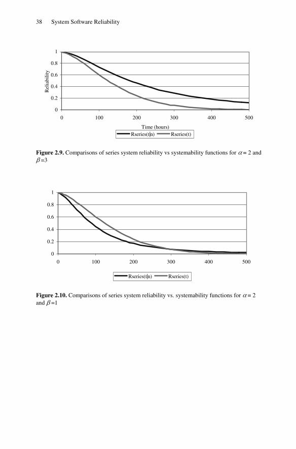
Figures 2.9 and 2.10 show the reliability function (conventional reliability function) and systemability function (equation 2.52) of a series system (here k=5) for 2, 3α β= = and for 2, 1α β= = , respectively.
Figures 2.11 and 2.12 show the reliability and systemability functions of a parallel system (here k=1) for 2, 3α β= = and for 2, 1α β= = , respectively.
Similarly, Figures 2.13 and 2.14 show the reliability and systemability functions of a 3-out-of-5 system for 2, 3α β= = and for 2, 1α β= = , respectively.
38 System Software Reliability
0
0.2
0.4
0.6
0.8
1
0 100 200 300 400 500
Time (hours)
Rel
iabi
lity
Rseries(t|n) Rseries(t)
Figure 2.9. Comparisons of series system reliability vs systemability functions for α = 2 and β =3
0
0.2
0.4
0.6
0.8
1
0 100 200 300 400 500
Rseries(t|n) Rseries(t)
Figure 2.10. Comparisons of series system reliability vs. systemability functions for α = 2 and β =1

System Reliability Concepts 39
0.8
0.84
0.88
0.92
0.96
1
0 100 200 300 400 500
Time (hours)
Rel
iab
ility
Rpara(t|n) Rpara(t)
Figure 2.11. Comparisons of parallel system reliability vs systemability function for α = 2 and β =3
0
0.2
0.4
0.6
0.8
1
0 100 200 300 400 500
Rpara(t|n) Rpara(t)
Figure 2.12. Comparisons of parallel system reliability vs Systemability functions for α = 2 and β =1

40 System Software Reliability
0
0.2
0.4
0.6
0.8
1
0 100 200 300 400 500
Time (hours)
Rel
iab
ility
Rkn(t|n) Rkn(t)
Figure 2.13. Comparisons of k-out-of-n system reliability vs. systemability functions for α = 2 and β =3
0
0.2
0.4
0.6
0.8
1
0 100 200 300 400 500
Rkn(t|n) Rkn(t)
Rkn(t)
Rkn(t|η)
Figure 2.14. Comparisons of k-out-of-n system reliability vs. systemability functions for α = 2 and β =1
Variance of Systemability Calculations Assume λ = 0.00001, γ = 1.5, n = 3, k = 2, and ~ ( , )η α βgamma , Figures 2.15
and 2.16 shows the systemability and its confidence intervals of a 2-out-of-3 system (Pham 1993) for 2, 1α β= = and 2, 2α β= = , respectively.

System Reliability Concepts 41
0.6
0.7
0.8
0.9
1
0 100 200 300 400 500Time (hours)
Rel
iabi
lity
Upper Bound
Lower Bound
RK -out-of-n (t )
Figure 2.15. A 2-out-of-3 systemability and its 95% confidence interval where α = 2, β = 1
0.8
0.85
0.9
0.95
1
0 100 200 300 400 500Time (hours)
Rel
iabi
lity
Lower Bound
Upper Bound
RK -out-of-n (t )
Figure 2.16. A 2-out-of-3 systemability and its 95% confidence interval (α = 2, β = 2)
2.4 System Reliability with Multiple Failure Modes
This section discusses various reliability and optimization aspects of systems subject to multiple types of failure. It is assumed that the system component states are statistically independent and identically distributed. Networks of relays, diode circuits, fluid flow valves, etc. are a few examples of systems having components subject to failure in either open or closed modes. The designations “closed mode” and “short mode” both appear in this section, and we will use the two terms interchangeably. Redundancy can be used to en-hance the reliability of a system without any change in the reliability of the

42 System Software Reliability
individual components that form the system. However, in a two-failure mode problem, redundancy may either increase or decrease the system's reliability. Therefore, adding components to the system may not increase the system reliability. The reliability of a system subject to two kinds of failure is calculated as follows (Malon 1989): System reliability = Pr{system works in both modes} (2.53) = Pr{system works in open mode} - Pr{system fails in closed mode}+ Pr{system fails in both modes) When the open- and closed-mode failure structures are dual of one another, i.e. Pr{system fails in both modes} = 0, then the system reliability given by equation (2.53) becomes System reliability = 1 - Pr{system fails in open mode} - Pr{system fails in closed mode} (2.54) Notation q0 The open-mode failure probability of each component (p0 = 1 - q0) qs The short-mode failure probability of each component (ps = 1 – qs) ⎢ ⎥⎣ ⎦x The largest integer not exceeding x
* Implies an optimal value
2.4.1 Reliability Calculations
The Series System Consider a series system consisting of n components. In this series system, any one component failing in an open mode causes system failure in open mode whereas all components of the system must malfunction in short mode for the system to fail in closed mode. The probabilities of system fails in open mode and fails in short mode are
0 0( ) 1 (1 )= − − nF n q
and
( ) = ns sF n q
respectively. From equation (2.54), the system reliability is
0( ) (1 )= − −n ns sR n q q (2.55)
where n is the number of identical and independent components. In a series arrangement, reliability with respect to closed system failure increases with the number of components, whereas reliability with respect to open system failure decreases.

System Reliability Concepts 43
Theorem 2.1: Let q0 and qs be fixed. There exists an optimum number of components, say n*, that maximizes the system reliability. If we define
0
0
0
log1
log1
⎛ ⎞⎜ ⎟−⎝ ⎠=⎛ ⎞⎜ ⎟−⎝ ⎠
s
s
q
qn
q
q
then the system reliability, Rs(n*), is maximum for
0 0
0 0 0
1 if is not an integer*
or 1 if is an integer
n nn
n n n
⎧ +⎢ ⎥⎪⎣ ⎦= ⎨+⎪⎩
(2.56)
Proof: The proof is left as an exercise for the reader (see Problem 2.17). Example 2.14: A switch has two failure modes: fail-open and fail-short. The probability of switch open-circuit failure and short-circuit failure are 0.1 and 0.2 respectively. A system consists of n switches wired in series. That is, given q0 = 0.1 and qs = 0.2. Then
0
0.1log
1 0.21.4
0.2log
1 0.1
⎛ ⎞⎜ ⎟−⎝ ⎠= =⎛ ⎞⎜ ⎟−⎝ ⎠
n
Thus, n* = 1.4⎢ ⎥⎣ ⎦ + 1 = 2. Therefore, when n* = 2 the system reliability Rs(n) =
0.77 is maximized. The Parallel System Consider a parallel system consisting of n components. For a parallel confi-guration, all the components must fail in open mode or at least one component must malfunction in short mode to cause the system to fail completely. The system reliability is given by
0( ) (1 )= − −n np sR n q q (2.57)
where n is the number of components connected in parallel. In this case, (1 – qs)n
represents the probability that no components fail in short mode, and q0n represents
the probability that all components fail in open mode. Theorem 2.2: If we define
00
0
log1
log1
⎛ ⎞⎜ ⎟−⎝ ⎠=⎛ ⎞⎜ ⎟−⎝ ⎠
s
s
q
qn
q
q
(2.58)

44 System Software Reliability
then the system reliability Rp(n*) is maximum for
0 0
0 0 0
1 if is not an integer*
or 1 if is an integer.
⎧ +⎢ ⎥⎪⎣ ⎦= ⎨+⎪⎩
n nn
n n n (2.59)
Proof: The proof is left as an exercise for the reader (see Problem 2.18). It is observed that, for any range of q0 and qs, the optimal number of parallel components that maximizes the system reliability is one, if qs > q0 (see Problem 2.19). For most other practical values of q0 and qs the optimal number turns out to be two. In general, the optimal value of parallel components can be easily obtained using equation (2.58). The Parallel-Series System Consider a system of components arranged so that there are m subsystems operating in parallel, each subsystem consisting of n identical components in series. Such an arrangement is called a parallel-series arrangement. The compo-nents are subject to two types of failure: failure in open mode and failure in short mode. The systems are characterized by the following properties: 1. The system consists of m subsystems, each subsystem containing n i.i.d. compo- nents. 2. A component is either good, failed open, or failed short. Failed components can never become good, and there are no transitions between the open and short failure modes. 3. The system can be (a) good, (b) failed open (at least one component in each subsystem fails open), or (c) failed short (all the components in any subsys-tem fail short). 4.The unconditional probabilities of component failure in open and short modes are known and are constrained: qo, qs > 0; qo + qs < 1. The probabilities of a system failing in open mode and failing in short mode are given by
0 0( ) [1 (1 ) ]= − − n mF m q (2.60)
and ( ) 1 (1 ( ) )= − − n ms sF m q (2.61)
respectively. The system reliability is
0( , ) (1 ) [1 (1 ) ]= − − − −n m n mps sR n m q q (2.62)
An interesting example in Barlow and Proschan (1965) shows that there exists no pair n, m maximizing system reliability, since Rps is made arbitrarily close to one by appropriate choice of m and n. To see this, let
/(1 )0
0
log log(1 )
log log(1 )− +− −
= = = ⎢ ⎥⎣ ⎦+ −n as
n s n ns
q qa M q m M
q q
System Reliability Concepts 45
For given n, take m = mn; then one can rewrite equation (2.62) as:
0( , ) (1 ) [1 (1 ) ]= − − − −n nm mn nps n sR n m q q
A straightforward computation yields
0lim ( , ) lim{(1 ) [1 (1 ) ] } 1→∞ →∞
= − − − − =n nm mn nps n s
n nR n m q q
For fixed n, q0, and qs, one can determine the value of m that maximizes Rps. Theorem 2.3 (Barlow and Proschan 1965): Let n, q0, and qs be fixed. The maximum value of Rps(m) is attained at 0* 1= +⎢ ⎥⎣ ⎦m m , where
00
0
(log log )
log(1 log(1 )
−=
− + −s
n ns
n p qm
q p (2.63)
If mo is an integer, then mo and mo+1 both maximize Rps(m). Proof: The proof is left as an exercise for the reader (see Problem 20). The Series-Parallel System The series-parallel structure is the dual of the parallel-series structure. We consider a system of components arranged so that there are m subsystems operating in series, each subsystem consisting of n identical components in parallel. Such an arrangement is called a series-parallel arrangement. Failure in open mode of all the components in any subsystem makes the system unresponsive. Failure in closed (short) mode of a single component in each subsystem also makes the system unresponsive. The probabilities of system failure in open and short mode are given by
0 0( ) 1 (1 )= − − n mF m q (2.64)
and
( ) [1 (1 ) ]= − − n ms sF m q (2.65)
respectively. The system reliability is
0( ) (1 ) [1 (1 ) ]= − − − −n m n msR m q q (2.66)
where m is the number of identical subsystems in series and n is the number of identical components in each parallel subsystem. Barlow and Proschan (1965) show that there exists no pair (m, n) maximizing system reliability. For fixed m, q0, and qs however, one can determine the value of n that maximizes the system reliability. Theorem 2.4 (Barlow and Proschan 1965): Let n, q0, and qs be fixed. The maximum value of R(m) is attained at 0* 1= +⎢ ⎥⎣ ⎦m m , where
00
0
(log log )
log(1 ) log(1 )
−=
− − −s
n ns
n p qm
q p (2.67)
If mo is an integer, then mo and mo + 1 both maximize R(m).

46 System Software Reliability
Proof: (see Problem 21). The k-out-of-n Systems Consider a k-out-of-n system consisting of n identical and independent components that can be either good or failed. The components are subject to two types of failure: failure in open mode and failure in closed mode. The k out of n system can fail when k or more components fail in closed mode or when (n - k + 1) or more components fail in open mode. Applications of k-out-of-n systems can be found in the areas of target detection, communication, and safety monitoring systems, and, particularly, in the area of human organizations. The following is an example in the area of human organizations (Nordmann and Pham 1999). Consider a committee with n members who must decide to accept or reject innovation-oriented projects. The projects are of two types: "good" and "bad". It is assumed that the communication among the members is limited, and each member will make a yes-no decision on each project. A committee member can make two types of error: the error of accepting a bad project and the error of rejecting a good project. The committee will accept a project when k or more members accept it, and will reject a project when (n - k + 1) or more members reject it. Thus, the two types of potential error of the committee are: (1) the acceptance of a bad project (which occurs when k or more members make the error of accepting a bad project); (2) the rejection of a good project (which occurs when (n - k + 1) or more members make the error of rejecting a good project). This section determines the optimal k or n that maximizes the system reliability. We also study the effect of the system's parameters on the optimal k or n. The system fails in closed mode if and only if at least k of its n components fail in closed mode, and we obtain
1
0
( , ) 1−
− −
= =
⎛ ⎞ ⎛ ⎞= = −⎜ ⎟ ⎜ ⎟
⎝ ⎠ ⎝ ⎠∑ ∑
n ki n i i n i
s s s s si k i
n nF k n q p q p
i i (2.68)
The system fails in open mode if and only if at least (n - k +1) of its n components fail in open mode, that is:
1
0 0 0 0 01 0
( , )−
− −
= − + =
⎛ ⎞ ⎛ ⎞= =⎜ ⎟ ⎜ ⎟
⎝ ⎠ ⎝ ⎠∑ ∑
n ki n i i n i
i n k i
n nF k n q p p q
i i (2.69)
The system reliability is given by
1 1
0 0 00 0
( , ) 1 ( , ) ( , )− −
− −
= =
⎛ ⎞ ⎛ ⎞= − − = −⎜ ⎟ ⎜ ⎟
⎝ ⎠ ⎝ ⎠∑ ∑k k
i n i i n is s s
i i
n nR k n F k n F k n q p p q
i i (2.70)
For a given k, we can find the optimum value of n, say n*, that maximizes the system reliability. Theorem 2.5 (Pham 1989a): For fixed k, q0, and qs, the maximum value of R(k, n) is attained at n* = 0⎢ ⎥⎣ ⎦n where

System Reliability Concepts 47
0
0
0
1log
11
log
⎡ ⎤⎛ ⎞−⎢ ⎥⎜ ⎟
⎝ ⎠⎢ ⎥= +⎢ ⎥⎛ ⎞−⎢ ⎥⎜ ⎟⎢ ⎥⎝ ⎠⎣ ⎦
s
s
q
qn k
q
q
(2.71)
If n0 is an integer, both n0 and n0 + 1 maximize R(k, n). Proof: The proof is left as an exercise for the reader (see Problem 22). This result shows that when n0 is an integer, both n*-1 and n* maximize the system reliability R(k, n). In such cases, the lower value will provide the more economical optimal configuration for the system. If q0 = qs the system reliability R(k, n) is maximized when n = 2k or 2k-1. In this case, the optimum value of n does not depend on the value of q0 and qs and the best choice for a decision voter is a majority voter; this system is also called a majority system (Pham,1989a).
From Theorem 2.5, we understand that the optimal system size n* depends on the various parameters q0 and qs. It can be shown the optimal value n* is an increasing function of q0 and a decreasing function of qs (see Problem 23). Intuitively, these results state that when qs increases it is desirable to reduce the number of components in the system as close to the value of threshold level k as possible. On the other hand, when q0 increases, the system reliability will be improved if the number of components increases. Theorem 2.6 (Ben-Dov 1980): For fixed n, q0, and qs, it is straightforward to see that the maximum value of R(k, n) is attained at k* = 0⎢ ⎥⎣ ⎦k +1, where
0
0
0
0
log
log
⎛ ⎞⎜ ⎟⎝ ⎠=⎛ ⎞⎜ ⎟⎝ ⎠
s
s
s
q
pk n
q q
p p
(2.72)
If k0 is an integer, both k0 and k0 + 1 maximize R(k, n). Proof: The proof is left as an exercise for the reader (see Problem 24).
We now discuss how these two values, k* and n*, are related to one another. Define α by
0
0
0
log
log
α
⎛ ⎞⎜ ⎟⎝ ⎠=⎛ ⎞⎜ ⎟⎝ ⎠
s
s
s
q
p
q q
p p
(2.73)
then, for a given n, the optimal threshold k is given by k* = nα⎡ ⎤⎢ ⎥ and for a given k the optimal n is n* = /α⎢ ⎥⎣ ⎦k . For any given q0 and qs, we can easily show that (see Problem 25)

48 System Software Reliability
0α< <sq p (2.74)
Therefore, we can obtain the following bounds for the optimal value of the threshold k:
0*< <snq k np (2.75)
This result shows that for given values of q0 and qs, an upper bound for the optimal threshold k* is the expected number of components working in open mode, and a lower bound for the optimal threshold k* is the expected number of components failing in closed mode.
2.4.2 An Application of Systems with Multiple Failure Modes
In many critical applications of digital systems, fault tolerance has been an essential architectural attribute for achieving high reliability. Several techniques can achieve fault tolerance using redundant hardware (Mathur and De Sousa 1975) or software (Pham 1985). Typical forms of redundant hardware structures for fault-tolerant systems are of two types: fault masking and standby. Masking redundancy is achieved by implementing the functions so that they are inherently error correcting, e.g. triple-modular redundancy (TMR), N-modular redundancy (NMR), and self-purging redundancy. In standby redundancy, spare units are switched into the system when working units break down. Mathur and De Sousa (1975) have analyzed, in detail, hardware redundancy in the design of fault-tolerant digital systems. Redundant software structures for fault-tolerant systems based on the acceptance tests have been proposed by Homing et al. (1974).
This section presents a fault-tolerant architecture to increase the reliability of a special class of digital systems in communication (Pham and Upadhyaya 1989b). In this system, a monitor and a switch are associated with each redundant unit. The switches and monitors can fail. The monitors have two failure modes: failure to accept a correct result, and failure to reject an incorrect result. The scheme can be used in communication systems to improve their reliability.
Consider a digital circuit module designed to process the incoming messages in a communication system. This module consists of two units: a converter to process the messages, and a monitor to analyze the messages for their accuracy. For example, the converter could be decoding or unpacking circuitry, whereas the monitor could be checker circuitry (Lala 1985).
To guarantee a high reliability of operation at the receiver end, n converters are arranged in "parallel". All, except converter n, have a monitor to determine if the output of the converter is correct. If the output of a converter is not correct, the output is cancelled and a switch is changed so that the original input message is sent to the next converter. The architecture of such a system has been proposed by Pham and Upadhyaya (1989b). Systems of this kind have useful applications in communication and network control systems and in the analysis of fault-tolerant software systems.
We assume that a switch is never connected to the next converter without a signal from the monitor, and the probability that it is connected when a signal arrives is ps. We next present a general expression for the reliability of the system

System Reliability Concepts 49
consisting of n non-identical converters arranged in "parallel". Let us define the following notation, events, and assumptions. Notation
cip Pr{converter i works} sip Pr{switch i is connected to converter (i + 1) when a signal arrives}
1mip Pr{monitor i works when converter i works} = Pr{not sending a signal to
the switch when converter i works} 2m
ip Pr{i monitor works when converter i has failed} = Pr{sending a signal to
the switch when converter i has failed}
−kn kR Reliability of the remaining system of size (n-k) given that the first k swit-
ches work
nR Reliability of the system consisting of n converters
The events are:
,w fi iC C Converter i works, fails
,w fi iM M Monitor i works, fails
,w fi iS S Switch i works, fails
W System works The assumptions are: 1. The system, the switches, and the converters are two-state: good or failed. 2. The module (converter, monitor, or switch) states are mutually statistically in- dependent. 3. The monitors have three states: good, failed in mode 1, failed in mode 2. 4. The modules are not identical.
The reliability of the system is defined as the probability of obtaining the correctly processed message at the output. To derive a general expression for the reliability of the system, we use an adapted form of the total probability theorem as translated into the language of reliability. Let A denote the event that a system performs as desired. Let Xi and Xj be the event that a component X (e.g. converter, monitor, or switch) is good or failed respectively. Then Pr{system works} = Pr{system works when unit X is good} x Pr{unit X is good}
+ Pr{system works when unit X fails} x Pr{unit X is failed} The above equation provides a convenient way of calculating the reliability of
complex systems. Notice that R1 = cip and for n ≥ 2, the reliability of the system
can be calculated as follows:
Rn = Pr{W | 1wC and 1
wM } Pr{ 1wC and 1
wM } + Pr{W | 1wC and 1
fM }
Pr{ 1wC and 1
fM } + Pr{W | 1fC and 1
wM } Pr{ 1fC and 1
wM }

50 System Software Reliability
+ Pr{W | 1fC and 1
fM } Pr{ 1fC and 1
fM }
In order for the system to operate when the first converter works and the first monitor fails, the first switch must work and the remaining system of size n-1 must work:
11 1 1 1Pr{ | and } −=w f s
nW C M p R
Similarly,
11 1 1 1Pr{ | and } −=f w s
nW C M p R
then
1 1 2 11 1 1 1 1 1 1 1[ (1 ) (1 ) ] −= + − + −m m mc c c s
n nR p p p p p p p R
The reliability of the system consisting of n non-identical converters can be rewritten as:
1
11 1
1
for 1π π−
− −=
= + >∑n
c m cn i i i n n
i
R p p p n (2.76)
and 1 1= cR p where
1
0
for 1
for all and 1
π
π π π=
= ≥
≡ =
∏k
jk i
i j
k k
A k
k
and
1 2[ (1 ) (1 ) ] for all 1, 2,....,≡ − + − =c m c mi i i i iA p p p p i n
Assume that all the converters, monitors, and switches have the same reliability, that is
1 1 2 2, , , for all = = = =c c m m m m s si i i ip p p p p p p p i
then we obtain a closed form expression for the reliability of system as follows:
1
1 1(1 )1
− −= − +−
c mn c n
n
p pR A p A
A (2.77)
where
1 2[ (1 ) (1 ) ]= − + −c m c m sA p p p p p
2.5 Markov Processes
Stochastic processes are used for the description of a systems operation over time. There are two main types of stochastic processes: continuous and discrete. The complex continuous process is a process describing a system transition from state to state. The simplest process that will be discussed here is a Markov process. Given the current state of the process, its future behavior does not depend on the past. In Section 2.6 we will discuss the discrete stochastic process. As an intro-duction to the Markov process, let us examine the following example.

System Reliability Concepts 51
Example 2.15: Consider a parallel system consisting of two components. From a reliability point of view, the states of the system can be described by
State 1: Full operation (both components operating) State 2: One component operating - one component failed State 3: Both components failed
Define
( ) [ ( ) ] [system is in state at time ]= = =iP t P X t i P i t
and
( ) [ ( ) ] [system is in state at time ].+ = + = = +iP t dt P X t dt i P i t dt
Define a random variable X(t) which can assume the values 1, 2, or 3 corresponding to the above-mentioned states. Since X(t) is a random variable, one can discuss P[X(t) = 1], P[X(t) = 2] or conditional probability, P[X(t1)= 2 | X(t0)= 1]. Again, X(t) is defined as a function of time t, the last stated conditional probability, P[X(t1)= 2 | X(t0)= 1], can be interpreted as the probability of being in state 2 at time t1, given that the system was in state 1 at time t0. In this example, the "stage space" is discrete, i.e., 1, 2, 3, etc., and the parameter space (time) is continuous. The simple process described above is called a stochastic process, i.e., a process which develops in time (or space) in accordance with some probabilistic (stochastic) laws. There are many types of stochastic processes. In this section, the emphasis will be on Markov processes which are a special type of stochastic process. Definition 2.3: Let t0 < t1 < ... < tn. If
1 1 2 2 0 0
1 1
[ ( ) | ( ) , ( ) ,...., ( ) ]
[ ( ) | ( ) ]− − − −
− −
= = = == = =
n n n n n n
n n n n
P X t A X t A X t A X t A
P X t A X t A
then the process is called a Markov process. Given the present state of the process, its future behavior does not depend on past information of the process. The essential characteristic of a Markov process is that it is a process that has no memory; its future is determined by the present and not the past. If, in addition to having no memory, the process is such that it depends only on the difference (t+dt)-t = dt and not the value of t, i.e., P[X(t + dt) = j | X(t) = i] is independent of t, then the process is Markov with stationary transition probabilities or homogeneous in time. This is the same property noted in exponential event times, and referring back to the graphical representation of X(t), the times between state changes would in fact be exponential if the process has stationary transition probabilities. Thus, a Markov process which is time homogeneous can be described as a process where events have exponential occurrence times. The random variable of the process is X(t), the state variable rather than the time to failure as in the exponential failure density. To see the types of processes that can be described, a review of the exponential distribution and its properties will be made. Recall that, if X1, X2,.…, Xn, are independent random variables, each with exponential density

52 System Software Reliability
and a mean equal to 1/λi then min { X1, X2, … , Xn} has an exponential density with
mean ( ) 1λ
−
∑ i .
The significance of the property is as follows: 1. The failure behavior of the simultaneous operation of components can be
characterized by an exponential density with a mean equal to the reciprocal of the sum of the failure rates.
2. The joint failure/repair behavior of a system where components are operating and/or undergoing repair can be characterized by an exponential density with a mean equal to the reciprocal of the sum of the failure and repair rates.
3. The failure/repair behavior of a system such as 2 above, but further complicated by active and dormant operating states and sensing and switching, can be characterized by an exponential density.
The above property means that almost all reliability and availability models can be characterized by a time homogeneous Markov process if the various failure times and repair times are exponential. The notation for the Markov process is {X(t), t>0}, where X(t) is discrete (state space) and t is continuous (parameter space). By convention, this type of Markov process is called a continuous parameter Markov chain. From a reliability/availability viewpoint, there are two types of Markov processes. These are defined as follows: 1. Absorbing Process: Contains what is called an "absorbing state" which is a
state from which the system can never leave once it has entered, e.g., a failure which aborts a flight or a mission.
2. Ergodic Process Contains no absorbing states such that X(t) can move around indefinitely, e.g., the operation of a ground power plant where failure only temporarily disrupts the operation. Pham (2000a) page 265, presents a summary of the processes to be considered
broken down by absorbing and ergodic categories. Both reliability and availability can be described in terms of the probability of the process or system being in defined "up" states, e.g., states 1 and 2 in the initial example. Likewise, the mean time between failures (MTBF) can be described as the total time in the “up” states before proceeding to the absorbing state or failure state. Define the incremental transition probability as
( ) [ ( ) | ( ) ]= + = =ijP dt P X t dt j X t i
This is the probability that the process (random variable X(t)) will go to state i during the increment t to (t+dt), given that it was in state i at time t. Since we are dealing with time homogeneous Markov processes, i.e., exponential failure and repair times, the incremental transition probabilities can be derived from an analy-sis of the exponential hazard function. In Section 2.1, it was shown that the hazard function for the exponential with mean 1/λ was just λ. This means that the limiting (as 0→dt ) conditional probability of an event occurrence between t and t + dt, given that an event had not occurred at time t, is just λ, i.e.,
System Reliability Concepts 53
0
[ | ]( ) lim λ
→
< < + >= =dt
P t X t dt X th t
dt
The equivalent statement for the random variable X(t) is
( ) [ ( ) | ( ) ] λ= + = = =h t dt P X t dt j X t i dt
Now, h(t)dt is in fact the incremental transition probability, thus the Pij(dt) can be stated in terms of the basic failure and/or repair rates.
Returning to Example 2.15, a state transition can be easily constructed showing the incremental transition probabilities for process between all possible states (see Figure.B.4, Pham 2000a)
State 1: Both components operating State 2: One component up - one component down State 3: Both components down (absorbing state)
The loops indicate the probability of remaining in the present state during the dt increment P11(dt) = 1 - 2λdt P12(dt) = 2λdt P13(dt) = 0 P21(dt) = 0 P22(dt) = 1 - λdt P23(dt) = λdt P31(dt) = 0 P32(dt) = 0 P33(dt) = 1 The zeros on Pij, i > j, denote that the process cannot go backwards, i.e., this is not a repair process. The zero on P13 denotes that in a process of this type, the probability of more than one event (e.g., failure, repair, etc.) in the incremental time period dt approaches zero as dt approaches zero. Except for the initial conditions of the process, i.e., the state in which the process starts, the process is completely specified by the incremental transition probabilities. The reason for the latter is that the assumption of exponential event (failure or repair) times allows the process to be characterized at any time t since it depends only on what happens between t and (t+dt). The incremental transition probabilities can be arranged into a matrix in a way which depicts all possible statewide movements. Thus, for the parallel configurations,
1 2 3
1 2 2 0[ ( )]
0 1
0 0 1
λ λλ λ
⎡ ⎤⎢ ⎥−⎢ ⎥=⎢ ⎥−⎢ ⎥⎣ ⎦
ij
dt dtp dt
dt dt
for i, j = 1, 2, or 3. The matrix [Pij(dt)] is called the incremental, one-step transition matrix. It is a stochastic matrix, i.e., the rows sum to 1.0. As mentioned earlier, this matrix along with the initial conditions completely describes the process. Now, [Pij(dt)] gives the probabilities for either remaining or moving to all the various states during the interval t to t + dt, hence,
P1(t + dt) = (1 - 2λdt)P1(t) P2(t + dt) = 2λdt P1(t)(1 - λdt)P2(t) P3(t + dt) = λdtP2(t) + P3(t)
By algebraic manipulation, we have

54 System Software Reliability
1 11
2 21 2
3 32
[ ( ) ( )]2 ( )
[ ( ) ( )]2 ( ) ( )
[ ( ) ( )]( )
λ
λ λ
λ
+ −= −
+ −= −
+ −=
P t dt P tP t
dtP t dt P t
P t P tdt
P t dt P tP t
dt
Taking limits of both sides as 0→dt , we obtain
P1’(t) = - 2λP1(t) P2’(t) = 2λP1(t) - 2λP2(t)
P3’(t) = λP2(t) The above system of linear first-order differential equations can be easily solved for P1(t) and P2(t), and therefore, the reliability of the configuration can be obtained:
2
1
( ) ( )=
=∑ ii
R t P t
Actually, there is no need to solve all three equations, but only the first two as P3(t) does not appear and also P3(t) = 1 – P1(t) – P2(t). The system of linear, first-order differential equations can be solved by various means including both manual and machine methods. For purposes here, the manual methods employing the Laplace transform (see Appendix 2) will be used.
0[ ( )] ( ) ( )
∞ −= =∫ sti i iL P t e P t dt f s
' '
0[ ( )] ( ) ( ) (0)
∞ −= = −∫ stii i iL P t e P t dt s f s P
The use of the Laplace transform will allow transformation of the system of linear, first-order differential equations into a system of linear algebraic equations which can easily be solved, and by means of the inverse transforms, solutions of Pi(t) can be determined. Returning to the example, the initial condition of the parallel configuration is assumed to be “full-up” such that P1(t = 0) = 1, P2(t = 0) = 0, P3(t = 0) = 0 transforming the equations for P’1(t) and P’2(t) gives
1 1 0 1
2 2 0 1 2
( ) ( ) | 2 ( )
( ) ( ) | 2 ( ) ( )
λλ λ
=
=
− = −− = −
t
t
sf s P t f s
sf s P t f s f s
Evaluating P1(t) and P2(t) at t = 0 gives
1 1
2 1 2
( ) 1 2 ( )
( ) 0 2 ( ) ( )
λλ λ
− = −− = −
sf s f s
sf s f s f s
from which we obtain
1
1 2
( 2 ) ( ) 1
2 ( ) ( ) ( ) 0
λλ λ+ =
− + + =s f s
f s s f s

System Reliability Concepts 55
Solving the above equations for f1(s) and f2(s), we have
1
2
1( )
( 2 )
2( )
[( 2 )( )]
λλ
λ λ
=+
=+ +
f ss
f ss s
From Appendix 2 of the inverse Laplace transforms,
21
22
21 2
( )
( ) 2 2
( ) ( ) ( ) 2
λ
λ λ
λ λ
−
− −
− −
=
= −
= + = −
t
t t
t t
P t e
P t e e
R t P t P t e e
The example given above is that of a simple absorbing process where we are concerned about reliability If repair capability in the form of a repair rate μ were added to the model, the methodology would remain the same with only the final result changing. With a repair rate μ added to the parallel configuration, the incremental transition matrix would be
1 2 2 0
[ ( )] 1 ( )
0 0 1
λ λμ λ μ λ
−⎡ ⎤⎢ ⎥= − +⎢ ⎥⎢ ⎥⎣ ⎦
ij
dt dt
P dt dt dt dt
The differential equations would become
P1’(t) = - 2λP1(t) + μP2(t) P2’(t) = 2λP1(t) – (λ +μ )P2(t)
and the transformed equations would become
1 2
1 2
( 2 ) ( ) ( ) 1
2 ( ) ( ) ( ) 0
λ μλ λ μ+ − =
− + + + =s f s f s
f s s f s
Hence, we obtain
1
1 2
21 2
( )( )
( )( )
2( )
( )( )
λ μ
λ
+ +=− −
=− −
sf s
s s s s
f ss s s s
where
2
1
2
2
(3 ) (3 )2 8
2
(3 ) (3 )2 8
2
λ μ λ μ λ
λ μ λ μ λ
− + + + −=
− + − + −=
s
s
From Appendix 2, we obtain
56 System Software Reliability
1 2
1 2
1 21
1 2 2 1
21 2 2 1
( ) ( )( )
( ) ( )
2 2( )
( ) ( )
λ μ λ μ
λ λ
− −
− −
+ + + += +
− −
= +− −
s t s t
s t s t
s e s eP t
s s s s
e eP t
s s s s
Thus, the reliability of two-component in a parallel system is given by
1 2
1 2
1 2
1 2
( ) ( ) ( )
( 3 ) ( 3 )
( )
λ μ λ μ− −
= +
+ + − + +=
−
s t s t
R t P t P t
s e s e
s s
(2.78)
System Mean Time Between Failures Another parameter of interest in absorbing Markov processes is the mean time between failures (MTBF). Recalling the previous example of a parallel configura-tion with repair, the differential equations P1'(t) and P2'(t) describing the process were
P1’(t) = - 2λP1(t) + μP2(t) P2’(t) = 2λP1(t) – (λ +μ )P2(t)
Integrating both sides of the above equations yields
1 1 2
0 0 0
' ( ) 2 ( ) ( )λ μ∞ ∞ ∞
= − +∫ ∫ ∫P t dt P t dt P t dt
'2 1 2
0 0 0
( ) 2 ( ) ( ) ( )λ λ μ∞ ∞ ∞
= − +∫ ∫ ∫P t dt P t dt P t dt
From Section 2.1,
0
( )∞
=∫ R t dt MTBF
Similarly,
1
0
2
0
( ) mean time spent in state 1, and
( ) mean time spent in state 2
∞
∞
=
=
∫
∫
P t dt
P t dt
Designating these mean times as T1 and T2, respectively, we have
1 0 1 2
2 0 1 2
( ) | 2
( ) | 2 ( )
λ μλ λ μ
∞
∞
= − +
= − +
P t dt T T
P t dt T T
But P1(t) = 0 as → ∞t and P1(t) = 1 for t = 0. Likewise, P2(t) = 0 as → ∞t and P2(t) = 0 for t = 0. Thus,

System Reliability Concepts 57
1 2
1 2
1 2
0 2 ( )
λ μλ λ μ
− = − += − +
T T
T T
or, equivalently,
1
2
1 2
0 2 ( )
λ μλ λ μ
− − ⎡ ⎤⎡ ⎤ ⎡ ⎤= ⎢ ⎥⎢ ⎥ ⎢ ⎥− +⎣ ⎦ ⎣ ⎦ ⎣ ⎦
T
T
Therefore,
1 22
1 2 2 2
( ) 1
2( ) 1 (3 )
2 2
λ μλλ
λ μ λ μλλ λ
+= =
+ += + = + =
T T
MTBF T T
The MTBF for non-maintenance processes is developed exactly the same way as just shown. What remains under absorbing processes is the case for availability for maintained systems. The difference between reliability and availability for absorbing processes is somewhat subtle. A good example is that of a communica-tion system where, if such a system failed temporarily, the mission would continue, but, if it failed permanently, the mission would be aborted. Consider the following cold-standby configuration consisting of two units: one main unit and one spare unit (Pham 2000a):
State 1: Main unit operating - spare OK State 2: Main unit out - restoration underway State 3: Spare unit installed and operating State 4: Permanent failure (no spare available)
The incremental transition matrix is given by (see Figure B.8 in Pham 2000a, for a detailed state transition diagram)
1 0 0
0 1 0[ ( )]
0 0 1
0 0 0 1
λ λμ μ
λ λ
−⎡ ⎤⎢ ⎥−⎢ ⎥=⎢ ⎥−⎢ ⎥⎣ ⎦
ij
dt dt
dt dtP dt
dt dt
We obtain
P1’(t) = - λP1(t) P2’(t) = λP1(t) - μP2(t)
P3’(t) = μP2(t) - λP3(t)
Using the Laplace transform, we obtain
1 1
2 1 2
3 2 3
( ) 1 ( )
( ) ( ) ( )
( ) ( ) ( )
λλ μμ λ
− = −= −= −
sf s f s
sf s f s f s
sf s f s f s
After simplifications,

58 System Software Reliability
1
2
3 2
1( )
( )
( )[( )( )]
( )[( ) ( )]
λλ
λ μλμ
λ μ
=+
=+ +
=+ +
f ss
f ss s
f ss s
Therefore, the probability of full-up performance, P1(t), is given by
1( ) λ−= tP t e
Similarly, the probability of the system being down and under repair, P2(t), is
( )2 ( )( )
μ λλλ μ
− −⎡ ⎤= −⎢ ⎥−⎣ ⎦
t tP t e e
and the probability of the system being full-up but no spare available, P3(t), is
3 2( ) [ ( ) ]
( )μ λ λλμ λ μ
λ μ− − −⎡ ⎤
= − − −⎢ ⎥−⎣ ⎦t t tP t e e te
Hence, the point availability, A(t), is given by
1 3( ) ( ) ( )= +A t P t P t
If average or interval availability is required, this is achieved by
1 3 0 0
1 1( ) [ ( ) ( )]
⎛ ⎞ ⎛ ⎞= +⎜ ⎟ ⎜ ⎟⎝ ⎠ ⎝ ⎠∫ ∫
T TA t dt P t P t dt
t t (2.79)
where T is the interval of concern. With the above example, cases of the absorbing process (both maintained and
non-maintained) have been covered insofar as "manual" methods are concerned. In general, the methodology for treatment of absorbing Markov processes can be “packaged” in a fairly simplified form by utilizing matrix notation. Thus, for exam-ple, if the incremental transition matrix is defined as follows:
1- 2 2 0
[ ( )] 1 ( )
0 0 1
λ λμ λ μ λ
⎡ ⎤⎢ ⎥= − +⎢ ⎥⎢ ⎥⎣ ⎦
ij
dt dt
P dt dt dt dt
then if the dts are dropped and the last row and the last column are deleted, the remainder is designated as the matrix T:
1- 2 2
[ ] 1 ( )
λ λμ λ μ
⎡ ⎤= ⎢ ⎥− +⎣ ⎦
T
Define [Q] = [T]' - [I], where [T]' is the transposition of [T] and [I] is the unity matrix:

System Reliability Concepts 59
1 2 1 0[ ]
2 1 ( ) 0 1
2
2 ( )
λ μλ λ μλ μλ λ μ
−⎡ ⎤ ⎡ ⎤= −⎢ ⎥ ⎢ ⎥− +⎣ ⎦ ⎣ ⎦
−⎡ ⎤= ⎢ ⎥− +⎣ ⎦
Q
Further define [P(t)] and [P’(t)] as column vectors such that
1 11
2 2
( ) '( )[ ( )] , [ '( )]
( ) '( )
⎡ ⎤ ⎡ ⎤= =⎢ ⎥ ⎢ ⎥⎣ ⎦ ⎣ ⎦
P t P tP t P t
P t P t
then
[ ] [ ][ ]'( ) ( )=P t Q P t
At the above point, solution of the system of differential equations will produce solutions to P1(t) and P2(t). If the MTBF is desired, integration of both sides of the system produces
1
2
1
2
11
2
1[ ]
0
1 2 or
0 2 ( )
1[ ]
0
λ μλ λ μ
−
− ⎡ ⎤⎡ ⎤= ⎢ ⎥⎢ ⎥
⎣ ⎦ ⎣ ⎦− − ⎡ ⎤⎡ ⎤ ⎡ ⎤
= ⎢ ⎥⎢ ⎥ ⎢ ⎥− +⎣ ⎦ ⎣ ⎦ ⎣ ⎦⎡ ⎤⎡ ⎤
= ⎢ ⎥⎢ ⎥⎣ ⎦ ⎣ ⎦
TQ
T
T
T
TQ
T
where [Q]-1 is the inverse of [Q] and the MTBF is given by
1 2 2
3MTBF
(2 )
λ μλ+= + =T T
In the more general MTBF case,
1
2
11
1
1
1
0
[ ] where MTBF
0
−−
=
−
− ⎡ ⎤⎡ ⎤⎢ ⎥⎢ ⎥⎢ ⎥⎢ ⎥⎢ ⎥⎢ ⎥⋅ ⋅
= =⎢ ⎥⎢ ⎥⋅ ⋅⎢ ⎥⎢ ⎥⎢ ⎥⎢ ⎥⋅ ⋅⎢ ⎥⎢ ⎥
⎢ ⎥ ⎢ ⎥⎣ ⎦ ⎣ ⎦
∑n
ii
n
T
T
Q T
T
and (n - 1) is the number of non-absorbing states. For the reliability/availability case, utilizing the Laplace transform, the system of linear, first-order differential equations is transformed to

60 System Software Reliability
1 1
2 2
1
2
1 1
2
11 1 1
2
1
2
( ) ( )1 [ ]
( ) 0 ( )
( ) 1[ ]
( ) 0
( ) 1 [ ]
( ) 0
( ) 1 {[ ] }
( ) 0
( )
( )
−
− − −
⎡ ⎤ ⎡ ⎤⎡ ⎤− =⎢ ⎥ ⎢ ⎥⎢ ⎥⎣ ⎦⎣ ⎦ ⎣ ⎦
⎡ ⎤ ⎡ ⎤− =⎢ ⎥ ⎢ ⎥
⎣ ⎦⎣ ⎦⎡ ⎤ ⎡ ⎤
= −⎢ ⎥ ⎢ ⎥⎣ ⎦⎣ ⎦
⎡ ⎤ ⎡ ⎤= −⎢ ⎥ ⎢ ⎥
⎣ ⎦⎣ ⎦⎡ ⎤⎢⎣ ⎦
f s f ss Q
f s f s
f ssI Q
f s
f ssI Q
f s
f sL L sI Q
f s
p s
p s1 1 1{[ ] }
0− − ⎡ ⎤= −⎥ ⎢ ⎥
⎣ ⎦L sI Q
Generalization of the latter to the case of (n-1) non-absorbing states is straightforward.
Ergodic processes, as opposed to absorbing processes, do not have any absorbing states, and hence, movement between states can go on indefinitely For the latter reason, availability (point, steady-state, or interval) is the only meaningful measure. As an example for ergodic processes, a ground-based power unit config-ured in parallel will be selected. The parallel units are identical, each with exponential failure and repair times with means 1/λ and 1/μ, respectively (Pham 2000a). Assume a two-repairmen capability if required (both units down), then
State 1: Full-up (both units operating) State 2: One unit down and under repair (other unit up) State 3: Both units down and under repair
It should be noted that, as in the case of failure events, two or more repairs cannot be made in the dt interval.
1 2 2 0
[ ( )] 1 ( )
0 2 1 2
λ λμ λ μ λ
μ μ
−⎡ ⎤⎢ ⎥= − +⎢ ⎥⎢ ⎥−⎣ ⎦
ij
dt dt
P dt dt dt dt
dt dt
Case I: Point Availability - Ergodic Process. For an ergodic process, as → ∞t the availability settles down to a constant level. Point availability gives a measure of things before the "settling down” and reflects the initial conditions on the process. Solution of the point availability is similar to the case for absorbing processes except that the last row and column of the transition matrix must be retained and entered into the system of equations. For example, the system of differential equations becomes
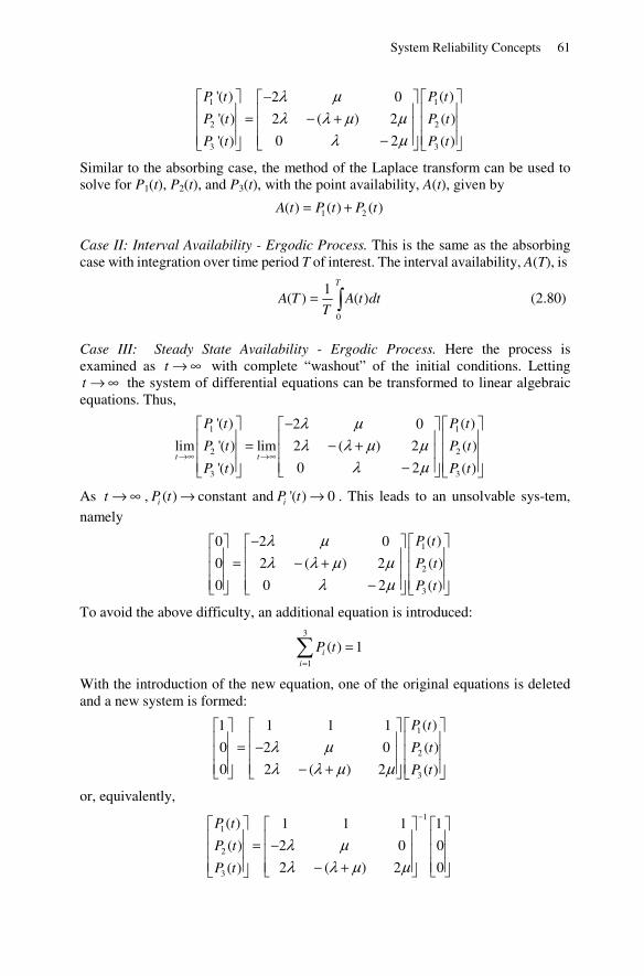
System Reliability Concepts 61
1 1
2 2
3 3
'( ) ( )2 0
'( ) 2 ( ) 2 ( )
0 2'( ) ( )
λ μλ λ μ μ
λ μ
−⎡ ⎤ ⎡ ⎤⎡ ⎤⎢ ⎥ ⎢ ⎥⎢ ⎥= − +⎢ ⎥ ⎢ ⎥⎢ ⎥⎢ ⎥ ⎢ ⎥⎢ ⎥−⎣ ⎦⎣ ⎦ ⎣ ⎦
P t P t
P t P t
P t P t
Similar to the absorbing case, the method of the Laplace transform can be used to solve for P1(t), P2(t), and P3(t), with the point availability, A(t), given by
1 2( ) ( ) ( )= +A t P t P t
Case II: Interval Availability - Ergodic Process. This is the same as the absorbing case with integration over time period T of interest. The interval availability, A(T), is
0
1( ) ( )= ∫
T
A T A t dtT
(2.80)
Case III: Steady State Availability - Ergodic Process. Here the process is examined as → ∞t with complete “washout” of the initial conditions. Letting
→ ∞t the system of differential equations can be transformed to linear algebraic equations. Thus,
1 1
2 2
3 3
'( ) ( )2 0
lim '( ) lim 2 ( ) 2 ( )
0 2'( ) ( )
λ μλ λ μ μ
λ μ→∞ →∞
−⎡ ⎤ ⎡ ⎤⎡ ⎤⎢ ⎥ ⎢ ⎥⎢ ⎥= − +⎢ ⎥ ⎢ ⎥⎢ ⎥⎢ ⎥ ⎢ ⎥⎢ ⎥−⎣ ⎦⎣ ⎦ ⎣ ⎦
t t
P t P t
P t P t
P t P t
As → ∞t , ( ) →iP t constant and '( ) 0→iP t . This leads to an unsolvable sys-tem,
namely
1
2
3
( )0 2 0
0 2 ( ) 2 ( )
0 0 2 ( )
λ μλ λ μ μ
λ μ
− ⎡ ⎤⎡ ⎤ ⎡ ⎤⎢ ⎥⎢ ⎥ ⎢ ⎥= − + ⎢ ⎥⎢ ⎥ ⎢ ⎥⎢ ⎥⎢ ⎥ ⎢ ⎥−⎣ ⎦ ⎣ ⎦ ⎣ ⎦
P t
P t
P t
To avoid the above difficulty, an additional equation is introduced:
3
1
( ) 1=
=∑ ii
P t
With the introduction of the new equation, one of the original equations is deleted and a new system is formed:
1
2
3
( )1 1 1 1
0 2 0 ( )
0 2 ( ) 2 ( )
λ μλ λ μ μ
⎡ ⎤⎡ ⎤ ⎡ ⎤⎢ ⎥⎢ ⎥ ⎢ ⎥= − ⎢ ⎥⎢ ⎥ ⎢ ⎥⎢ ⎥⎢ ⎥ ⎢ ⎥− +⎣ ⎦ ⎣ ⎦ ⎣ ⎦
P t
P t
P t
or, equivalently,
11
2
3
( ) 1 1 1 1
( ) 2 0 0
2 ( ) 2 0( )
λ μλ λ μ μ
−⎡ ⎤ ⎡ ⎤ ⎡ ⎤⎢ ⎥ ⎢ ⎥ ⎢ ⎥= −⎢ ⎥ ⎢ ⎥ ⎢ ⎥⎢ ⎥ ⎢ ⎥ ⎢ ⎥− +⎣ ⎦ ⎣ ⎦⎣ ⎦
P t
P t
P t
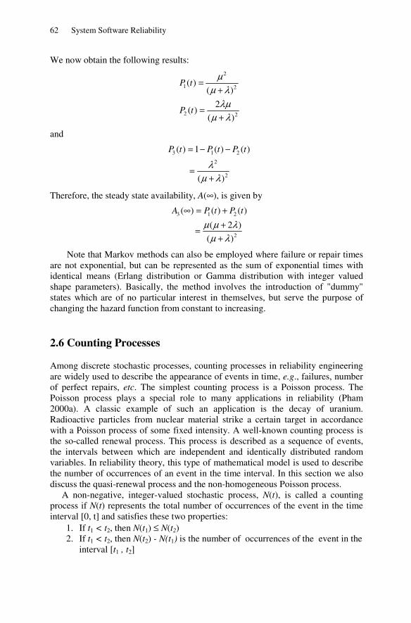
62 System Software Reliability
We now obtain the following results:
2
1 2
2 2
( )( )
2( )
( )
μμ λ
λμμ λ
=+
=+
P t
P t
and
3 1 2
2
2
( ) 1 ( ) ( )
( )
λμ λ
= − −
=+
P t P t P t
Therefore, the steady state availability, A(∞), is given by
3 1 2
2
( ) ( ) ( )
( 2 )
( )
μ μ λμ λ
∞ = ++=
+
A P t P t
Note that Markov methods can also be employed where failure or repair times are not exponential, but can be represented as the sum of exponential times with identical means (Erlang distribution or Gamma distribution with integer valued shape parameters). Basically, the method involves the introduction of "dummy" states which are of no particular interest in themselves, but serve the purpose of changing the hazard function from constant to increasing.
2.6 Counting Processes
Among discrete stochastic processes, counting processes in reliability engineering are widely used to describe the appearance of events in time, e.g., failures, number of perfect repairs, etc. The simplest counting process is a Poisson process. The Poisson process plays a special role to many applications in reliability (Pham 2000a). A classic example of such an application is the decay of uranium. Radioactive particles from nuclear material strike a certain target in accordance with a Poisson process of some fixed intensity. A well-known counting process is the so-called renewal process. This process is described as a sequence of events, the intervals between which are independent and identically distributed random variables. In reliability theory, this type of mathematical model is used to describe the number of occurrences of an event in the time interval. In this section we also discuss the quasi-renewal process and the non-homogeneous Poisson process. A non-negative, integer-valued stochastic process, N(t), is called a counting process if N(t) represents the total number of occurrences of the event in the time interval [0, t] and satisfies these two properties: 1. If t1 < t2, then N(t1) ≤ N(t2) 2. If t1 < t2, then N(t2) - N(t1) is the number of occurrences of the event in the interval [t1 , t2]
System Reliability Concepts 63
For example, if N(t) equals the number of persons who have entered a restaurant at or prior to time t, then N(t) is a counting process in which an event occurs whenever a person enters the restaurant.
2.6.1 Poisson Processes
One of the most important counting processes is the Poisson process. Definition 2.4: A counting process, N(t), is said to be a Poisson process with intensity λ if 1. The failure process, N(t), has stationary independent increments 2. The number of failures in any time interval of length s has a Poisson distribution with mean λs, that is,
( )
{ ( ) ( ) } 0,1, 2,...!
λ λ−
+ − = = =s ne s
P N t s N t n nn
(2.81)
3. The initial condition is N(0) = 0 This model is also called a homogeneous Poisson process indicating that the failure rate λ does not depend on time t. In other words, the number of failures occurring during the time interval (t, t + s] does not depend on the current time t but only the length of time interval s. A counting process is said to possess independent incre-ments if the number of events in disjoint time intervals are independent. For a stochastic process with independent increments, the auto-covariance function is
1 2 2 11 2
[ ( ) ( )] for 0[ ( ), ( )]
0 otherwise
+ − < − <⎧= ⎨⎩
Var N t s N t t t sCov X t X t
where
( ) ( ) ( ).= + −X t N t s N t
If X(t) is Poisson distributed, then the variance of the Poisson distribution is
2 1 2 11 2
[ ( )] for 0[ ( ), ( )]
0 otherwise
λ − − < − <⎧= ⎨⎩
s t t t t sCov X t X t
This result shows that the Poisson increment process is covariance stationary. We now present several properties of the Poisson process. Property 2.3: The sum of independent Poisson processes, N1(t), N2(t), …., Nk(t), with mean values λ1t, λ2t, …., λkt respectively, is also a Poisson process with mean
1
λ=
⎛ ⎞⎜ ⎟⎝ ⎠∑
k
ii
t . In other words, the sum of the independent Poisson processes is also a
Poisson process with a mean that is equal to the sum of the individual Poisson process' mean. Proof: The proof is left as an exercise for the reader (see Problem 26).

64 System Software Reliability
Property 2.4: The difference of two independent Poisson processes, N1(t), and N2(t), with mean λ1t and λ2t, respectively, is not a Poisson process. Instead, it has the probability mass function
1 2
2( ) 1
1 2 1 22
[ ( ) ( ) ] (2 )λ λ λ λ λλ
− + ⎛ ⎞− = = ⎜ ⎟
⎝ ⎠
k
tkP N t N t k e I t (2.82)
where Ik(.) is a modified Bessel function of order k (Handbook 1980). Proof: The proof is left as an exercise for the reader (see Problem 27). Property 2.5: If the Poisson process, N(t), with mean λt, is filtered such that every occurrence of the event is not completely counted, then the process has a constant probability p of being counted. The result of this process is a Poisson process with mean λpt [ ]. Property 2.6: Let N(t) be a Poisson process and Yn a family of independent and identically distributed random variables which are also independent of N(t). A stochastic process X(t) is said to be a compound Poisson process if it can be represented as
( )
1
( )=
= ∑N t
ii
X t Y
2.6.2 Renewal Processes
A renewal process is a more general case of the Poisson process in which the inter-arrival times of the process or the time between failures do not necessarily follow the exponential distribution. For convenience, we will call the occurrence of an event a renewal, the inter-arrival time the renewal period, and the waiting time the renewal time. Definition 2.5: A counting process N(t) that represents the total number of occurrences of an event in the time interval (0, t] is called a renewal process, if the time between failures are independent and identically distributed random variables. The probability that there are exactly n failures occurring by time t can be written as
{ ( ) } { ( ) } { ( ) }= = ≥ − >P N t n P N t n P N t n (2.83)
Note that the times between the failures are T1, T2, …, Tn so the failures occurring at time Wk are
1=
=∑k
k ii
W T
and
1−= −k k kT W W

System Reliability Concepts 65
Thus,
1
1
{ ( ) } { ( ) } { ( ) }
{ } { }
( ) ( )+
+
= = ≥ − >= ≤ − ≤= −
n n
n n
P N t n P N t n P N t n
P W t P W t
F t F t
where Fn(t) is the cumulative distribution function for the time of the nth failure and n = 0,1,2, ... . Example 2.16: Consider a software testing model for which the time to find an error during the testing phase has an exponential distribution with a failure rate of X. It can be shown that the time of the nth failure follows the gamma distribution with parameters k and n with probability density function. From equation (2.83) we obtain
1
0 0
{ ( ) } { ( ) } { ( ) 1}
( ) ( )
! !
( ) for 0,1,2,....
!
λ λ
λ
λ λ
λ
−− −
= =
−
= = ≤ − ≤ −
= −
= =
∑ ∑k kn n
t t
k k
nt
P N t n P N t n P N t n
t te e
k k
te n
n
Several important properties of the renewal function are given below. Property 2.7: The mean value function of the renewal process, denoted by m(t), is equal to the sum of the distribution function of all renewal times, that is,
1
( ) [ ( )]
( )∞
=
=
=∑ nn
m t E N t
F t
Proof: The renewal function can be obtained as
1
11
1
( ) [ ( )]
{ ( ) }
[ ( ) ( )]
( )
∞
=∞
+=∞
=
=
= =
= −
=
∑
∑
∑
n
n nn
nn
m t E N t
nP N t n
n F t F t
F t
The mean value function of the renewal process is also called the renewal function. Property 2.8: The renewal function, m(t), satisfies the following equation:

66 System Software Reliability
0
( ) ( ) ( ) ( )= + −∫t
a am t F t m t s dF s (2.84)
where Fa(t) is the distribution function of the inter-arrival time or the renewal period. The proof is left as an exercise for the reader (see Problem 28).
In general, let y(t) be an unknown function to be evaluated and x(t) be any non-negative and integrable function associated with the renewal process. Assume that Fa(t) is the distribution function of the renewal period. We can then obtain the following result. Property 2.9: Let the renewal equation be
0
( ) ( ) ( ) ( )= + −∫t
ay t x t y t s dF s (2.85)
then its solution is given by
0
( ) ( ) ( ) ( )= + −∫t
y t x t x t s dm s
where m(t) is the mean value function of the renewal process. The proof of the above property can be easily derived using the Laplace
transform. It is also noted that the integral equation given in Property 2.8 is a special case of Property 2.9. Example 2.17: Let x(t) = a. Thus, in Property 2.9, the solution y(t) is given by
0
0
( ) ( ) ( ) ( )
( )
(1 [ ( )])
= + −
= +
= +
∫
∫
t
t
y t x t x t s dm s
a a dm s
a E N t
2.6.3 Quasi-renewal Processes
In this section, a general renewal process, namely, the quasi-renewal process, is discussed. Let {N(t), t > 0} be a counting process and let Xn be the time between the (n-1)th and the nth event of this process, n ≥ 1. Definition 2.6 (Wang and Pham 1996a): If the sequence of non-negative random variables {X1, X2, ....} is independent and
1−=i iX aX (2.86)
for i ≥ 2 where α > 0 is a constant, then the counting process {N(t), t ≥ 0} is said to be a quasi-renewal process with parameter and the first inter-arrival time X1.

System Reliability Concepts 67
When α = 1, this process becomes the ordinary renewal process as discussed in Section 2.6.2. This quasi-renewal process can be used to model reliability growth processes in software testing phases and hardware burn-in stages for α > 1, and in hardware maintenance processes when α ≤ 1. Assume that the probability density function, cumulative distribution function, survival function, and failure rate of random variable X1 are f1(x), F1(x), s1(x), and r1(x), respectively. Then the pfd, cdf, survival function, failure rate of Xn for n = 1, 2, 3,... is respectively given below (Wang and Pham 1996a):
11 1
1 1
1 1
11 1
1 1( )
1( )
1( )
1 1( )
α α
α
α
α α
− −
−
−
− −
⎛ ⎞= ⎜ ⎟⎝ ⎠
⎛ ⎞= ⎜ ⎟⎝ ⎠⎛ ⎞= ⎜ ⎟⎝ ⎠
⎛ ⎞= ⎜ ⎟⎝ ⎠
n n n
n n
n n
n n n
f x f x
F x F x
s x s x
f x r x
Similarly, the mean and variance of Xn is given as
1
1
2 21
( ) ( )
( ) ( )
αα
−
−
=
=
nn
nn
E X E X
Var X Var X
Because of the non-negativity of X1 and the fact that X1 is not identically 0, we obtain
1 1( ) 0μ= ≠E X
Proposition 2.1 (Wang and Pham 1996a): The shape parameters of Xn are the same for n = 1, 2, 3, ... for a quasi-renewal process if X1 follows the gamma, Weibull, or log normal distribution.
This means that after "renewal", the shape parameters of the inter-arrival time will not change. In software reliability, the assumption that the software debugging process does not change the error-free distribution type seems reasonable. Thus, the error-free times of software during the debugging phase modeled by a quasi-renewal process will have the same shape parameters. In this sense, a quasi-renewal process is suitable to model the software reliability growth. It is worthwhile to note that
1 2 1( ... ) (1 )lim lim
(1 )
0 if 1
if 1
μ αα
αα
→∞ →∞
+ + + −=
−= <= ∞ >
nn
n n
E X X X
n n
68 System Software Reliability
Therefore, if the inter-arrival time represents the error-free time of a software system, then the average error-free time approaches infinity when its debugging process is occurring for a long debugging time. Distribution of N(t) Consider a quasi-renewal process with parameter α and the first inter-arrival time X1. Clearly, the total number of renewals, N(t), that has occurred up to time t and the arrival time of the nth renewal, SSn, has the following relationship:
N(t) ≥ n if and only if SSn ≤ t
that is, N(t) is at least n if and only if the nth renewal occurs prior to time t. It is easily seen that
11
1 1
for 1α −
= =
= = ≥∑ ∑n n
in i
i i
SS X X n (2.87)
Here, SS0 = 0. Thus, we have
1
1
{ ( ) } { ( ) } { ( ) 1}
{ } { }
( ) ( )+
+
= = = − ≥ += ≤ − ≤= −
n n
n n
P N t n P N t n P N t n
P SS t P SS t
G t G t
where Gn(t) is the convolution of the inter-arrival times F1, F2, F3, …, Fn. In other words,
1 2( ) { .... }= + + + ≤n nG t P F F F t
If the mean value of N(t) is defined as the renewal function m(t), then,
1
1
1
( ) [ ( )]
{ ( ) }
{ }
( )
∞
=∞
=∞
=
=
= ≥
= ≤
=
∑
∑
∑
n
nn
nn
m t E N t
P N t n
P SS t
G t
The derivative of m(t) is known as the renewal density
( ) '( )λ =t m t
In renewal theory, random variables representing the inter-arrival distributions only assume non-negative values, and the Laplace transform of its distribution F1(t) is defined by
1 1
0
{ ( )} ( )∞
−= ∫ sxF s e dF xL
Therefore,
a 1 11 1
0
( ) ( ) ( )α−
∞− −= =∫
n st nnF s e dF t F sL L

System Reliability Concepts 69
and
1
11 1 1
1
( ) ( )
( ) ( ) ( )α α
∞
=∞
−
=
=
= ⋅⋅ ⋅ ⋅
∑
∑
n nn
n
n
m s G s
F s F s F s
L L
L L L
Since there is a one-to-one correspondence between distribution functions and its Laplace transform, it follows that Proposition 2.2 (Wang and Pham 1996a): The first inter-arrival distribution of a quasi-renewal process uniquely determines its renewal function.
If the inter-arrival time represents the error-free time (time to first failure), a quasi-renewal process can be used to model reliability growth for both software and hardware.
Suppose that all faults of software have the same chance of being detected. If the inter-arrival time of a quasi-renewal process represents the error-free time of a software system, then the expected number of software faults in the time interval [0, t] can be defined by the renewal function, m(t), with parameter α > 1. Denoted by mr(t), the number of remaining software faults at time t, it follows that
( ) ( ) ( )= −r cm t m T m t
where m(Tc) is the number of faults that will eventually be detected through a software lifecycle Tc.
2.6.4 Non-homogeneous Poisson Processes
The non-homogeneous Poisson process model (NHPP) that represents the number of failures experienced up to time t is a non-homogeneous Poisson process {N(t), t ≥ 0}. The main issue in the NHPP model is to determine an appropriate mean value function to denote the expected number of failures experienced up to a certain time. With different assumptions, the model will end up with different functional forms of the mean value function. Note that in a renewal process, the exponential assumption for the inter-arrival time between failures is relaxed, and in the NHPP, the stationary assumption is relaxed.
The NHPP model is based on the following assumptions: • The failure process has an independent increment, i.e., the number of failures
during the time interval (t, t + s) depends on the current time t and the length of time interval s, and does not depend on the past history of the process.
• The failure rate of the process is given by
{exactly one failure in ( , )} { ( ) ( ) 1}
( ) ( )λ+ Δ = + Δ − =
= Δ + ΔP t t t P N t t N t
t t o t
where λ(t) is the intensity function. • During a small interval Δt, the probability of more than one failure is
negligible, that is,

70 System Software Reliability
{two or more failure in ( , )} ( )+ Δ = ΔP t t t o t
• The initial condition is N(0) = 0. On the basis of these assumptions, the probability of exactly n failures occurring during the time interval (0, t) for the NHPP is given by
( )[ ( )]Pr{ ( ) } 0,1, 2,...
!−= = =
nm tm t
N t n e nn
(2.88)
where 0
( ) [ ( )] ( )λ= = ∫t
m t E N t s ds and λ(t) is the intensity function. It can be easily
shown that the mean value function m(t) is non-decreasing. Reliability Function The reliability R(t), defined as the probability that there are no failures in the time interval (0, t), is given by
( )
( ) { ( ) 0}
−
= =
= m t
R t P N t
e
In general, the reliability R(x|t), the probability that there are no failures in the interval (t, t + x), is given by
[ ( ) ( )]
( | ) { ( ) ( ) 0}
− + −
= + − =
= m t x m t
R x t P N t x N t
e
and its density is given by
[ ( ) ( )]( ) ( )λ − + −= + m t x m tf x t x e
where
( ) [ ( )]λ ∂=∂
x m xx
The variance of the NHPP can be obtained as follows:
0
[ ( )] ( )λ= ∫t
Var N t s ds
and the auto-correlation function is given by
2
0 0 0
0 0
[ ] [ ( )] [ ( ) ( )] [ ( )]
( ) ( ) ( )
( ) 1 ( )
λ λ λ
λ λ
+
+
= + − +
= +
⎡ ⎤= +⎢ ⎥
⎢ ⎥⎣ ⎦
∫ ∫ ∫
∫ ∫
t t s t
t t s
Cor s E N t E N t s N t E N t
s ds s ds s ds
s ds s ds

System Reliability Concepts 71
Example 2.18: Assume that the intensity λ is a random variable with the pdf f(λ). Then the probability of exactly n failures occurring during the time interval (0, t) is given by
0
( ){ ( ) } ( )
!λ λ λ λ
∞−= = ∫
nt t
P N t n e f dn
It can be shown that if the pdf f(λ) is given as the following gamma density function with parameters k and m,
11( ) for 0
( )λλ λ λ− −= ≥
Γm m kf k e
m
then
1
{ ( ) } 0,1, 2,...+ −⎛ ⎞
= = =⎜ ⎟⎝ ⎠
m nn mP N t n p q n
n
is also called a negative binomial density function, where
and 1= = = −+ +k t
p q pt k t k
2.7 Further Reading
The reader interested in a deeper understanding of advanced probability theory and stochastic processes should note the following highly recommended books: Devore, J.L., Probability and Statistics for Engineering and the Sciences, 3rd edition, Brooks/Cole Pub. Co., Pacific Grove, 1991. Gnedenko, BV and I.A. Ushakov, Probabilistic Reliability Engineering, Wiley, New York, 1995. Feller, W., An Introduction to Probability Theory and Its Applications, 3rd edition, Wiley, New York, 1994.
2.8 Problems
1. Assume that the hazard rate, h(t), has a positive derivative. Show that the hazard distribution
0
( ) ( )= ∫t
H t h x dx
is strictly convex. 2. An operating unit is supported by (n-1) identical units on cold standby. When
it fails, a unit from standby takes its place. The system fails if all n units fail.

72 System Software Reliability
Assume that units on standby cannot fail and the lifetime of each unit follows the exponential distribution with failure rate λ . (a) What is the distribution of the system lifetime? (b) Determine the reliability of the standby system for a mission of 100
hours when λ = 0.0001 per hour and n = 5. 3. Assume that there is some latent deterioration process occurring in the
system. During the interval [0, a-h] the deterioration is comparatively small so that the shocks do not cause system failure. During a relatively short time interval [a-h, a], the deterioration progresses rapidly and makes the system susceptible to shocks. Assume that the appearance of each shock follows the exponential distribution with failure rate λ . What is the distribution of the system lifetime?
4. Consider a series system of n Weibull components. The corresponding
lifetimes T1, T2,..., Tn are assumed to be independent with pdf
( )1 for 0
( )0 otherwise
βλβ βλ β −−⎧ ≥⎪= ⎨⎪⎩
i ti t e t
f t
where λ > 0 and β > 0 are the scale and shape parameters, respectively.
(a) Show that the lifetime of a series system has the Weibull distribution
with pdf
11
1
for 0( )
0 otherwise
β βλβ βλ β =
⎛ ⎞−⎜ ⎟⎜ ⎟− ⎝ ⎠
=
⎧ ∑⎛ ⎞⎪ ≥⎜ ⎟= ⎨⎝ ⎠⎪⎩
∑n
ii
n t
is i
t e tf t
(b) Find the reliability of this series system. 5. Consider the pdf of a random variable that is equally likely to take on any value only in the interval from a to b. (a) Show that this pdf is given by
1
for 0( )
0 otherwise
⎧ < <⎪= −⎨⎪⎩
a tf t b a
(b) Derive the corresponding reliability function R(t) and failure rate h(t). (c) Think of an example where such a distribution function would be of
interest in reliability application. 6. The failure rate function, denoted by h(t), is defined as
( ) ln[ ( )]= − dh t R t
dt

System Reliability Concepts 73
Show that the constant failure rate function implies an exponential distribution.
7. One thousand new streetlights are installed in Saigon city. Assume that the
lifetimes of these streetlights follow the normal distribution. The average life of these lamps is estimated at 980 burning-hours with a standard deviation of 100 hours. (a) What is the expected number of lights that will fail during the first 800
burning-hours? (b) What is the expected number of lights that will fail between 900 and
1100 burning-hours? (c) After how many burning-hours would 10% of the lamps be expected to
fail? 8. A fax machine with constant failure rate λ will survive for a period of 720
hours without failure, with probability 0.80. (a) Determine the failure rate λ . (b) Determine the probability that the machine, which is functioning after
600 hours, will still function after 800 hours. (c) Find the probability that the machine will fail within 900 hours, given
that the machine was functioning at 720 hours. 9. The time to failure T of a unit is assumed to have a log normal distribution
with pdf
2
2
(ln )
21 1
( ) 02
μσ
σπ
−−= >
t
f t e tt
Show that the failure rate function is unimodal. 10. A diode may fail due to either open or short failure modes. Assume that the
time to failure T0 caused by open mode is exponentially distributed with pdf
0
0 0( ) 0λλ −= ≥tf t e t
and the time to failure T1 caused by short mode has the pdf
( ) 0λλ −= ≥sts sf t e t
The pdf for the time to failure T of the diode is given by
0( ) ( ) (1 ) ( ) 0= + − ≥sf t p f t p f t t
(a) Explain the meaning of p in the above pdf function. (b) Derive the reliability function R(t) and failure rate function h(t) for the
time to failure T of the diode. (c) Show that the diode with pdf f(t) has a decreasing failure rate (DFR).
11. A diesel is known to have an operating life (in hours) that fits the following pdf:
74 System Software Reliability
2
2( ) 0
( )= ≥
+a
f t tt b
The average operating life of the diesel has been estimated to be 8760 hours. (a) Determine a and b. (b) Determine the probability that the diesel will not fail during the first
6000 operating-hours. (c) If the manufacturer wants no more than 10% of the diesels returned for
warranty service, how long should the warranty be? 12. The failure rate for a hydraulic component
( ) 01
= >+t
h t tt
where t is in years. (a) Determine the reliability function R(t). (b) Determine the MTTF of the component.
13. A 18-month guarantee is given based on the assumption that no more than 5% of new cars will be returned.
(a) The time to failure T of a car has a constant failure rate. What is the maximum failure rate that can be tolerated?
(b) Determine the probability that a new car will fail within three years assuming that the car was functioning at 18 months.
14. Show that if
1 2( ) ( ) for all ≥R t R t t
where Ri(t) is the system reliability of the structure i, then MTTF of the system structure 1 is always ≥ MTTF of the system structure 2.
15. Prove equation (2.10) 16. Show that the reliability function of Pham distribution (see equation 2.21) is
given as in equation (2.22). 17. Prove Theorem 2.1. 18. Prove Theorem 2.2. 19. Show that for any range of q0 and qs, if qs > q0, the optimal number of parallel components that maximizes the system reliability is one. 20. Prove Theorem 2.3. 21. Prove Theorem 2.4. 22. Prove Theorem 2.5.

System Reliability Concepts 75
23. Show that the optimal value n* in Theorem 2.5 is an increasing function of q0 and a decreasing function of qs.
24. Prove Theorem 2.6. 25. For any given q0 and qs, show that 0α< <sq p whereα is given in equation
(2.73). 26. Prove Property 2.3. 27. Prove Property 2.4. 28. Prove Property 2.8. 29. Events occur according to an NHPP in which the mean value function is
m(t) = t3 + 3t2 + 6t t > 0.
What is the probability that n events occur between times t = 10 and t = 15?

http://www.springer.com/978-1-85233-950-0