General rights Copyright and moral rights for the publications made accessible in the public portal are retained by the authors and/or other copyright owners and it is a condition of accessing publications that users recognise and abide by the legal requirements associated with these rights.

• Users may download and print one copy of any publication from the public portal for the purpose of private study or research. • You may not further distribute the material or use it for any profit-making activity or commercial gain • You may freely distribute the URL identifying the publication in the public portal

If you believe that this document breaches copyright please contact us providing details, and we will remove access to the work immediately and investigate your claim.

Downloaded from orbit.dtu.dk on: Jun 24, 2018

System-Level Modeling and Synthesis Techniques for Flow-Based Microfluidic VeryLarge Scale Integration Biochips

Minhass, Wajid Hassan; Pop, Paul; Madsen, Jan

Publication date:2012

Document VersionPublisher's PDF, also known as Version of record

Link back to DTU Orbit

Citation (APA):Minhass, W. H., Pop, P., & Madsen, J. (2012). System-Level Modeling and Synthesis Techniques for Flow-Based Microfluidic Very Large Scale Integration Biochips. Kgs. Lyngby: Technical University of Denmark (DTU).(IMM-PhD-2012; No. 286).

System-Level Modeling andSynthesis Techniques for

Flow-Based Microfluidic Very LargeScale Integration Biochips

Wajid Hassan Minhass

Kongens Lyngby 2012

IMM-PHD-2012-286

Technical University of Denmark

Informatics and Mathematical Modelling

Building 321, DK-2800 Kongens Lyngby, Denmark

Phone +45 45253351, Fax +45 45882673

reception@imm.dtu.dk

www.imm.dtu.dk

IMM-PHD: ISSN 0909-3192

To My Parents

Summary

Microfluidic biochips integrate different biochemical analysis functionalities on-chip and offer several advantages over the conventional biochemical laboratories.In this thesis, we focus on the flow-based biochips. The basic building blockof such a chip is a valve which can be fabricated at very high densities, e.g.,1 million valves per cm2. By combining these valves, more complex units suchas mixers, switches, multiplexers can be built up and the technology is thereforereferred to as microfluidic Very Large Scale Integration (mVLSI).

The manufacturing technology for the mVLSI biochips has advanced faster thanMoore’s law. However, the design methodologies are still manual and bottom-up. Designers use drawing tools, e.g., AutoCAD, to manually design the chip. Inorder to run the experiments, applications are manually mapped onto the valvesof the chips (analogous to exposure of gate-level details in electronic integratedcircuits). Since mVLSI chips can easily have thousands of valves, the manualprocess can be very time-consuming, error-prone and result in inefficient designsand mappings.

We propose, for the first time to our knowledge, a top-down modeling andsynthesis methodology for the mVLSI biochips. We propose a modeling frame-work for the components and the biochip architecture. Using these models,we present an architectural synthesis methodology (covering steps from theschematic design to the physical synthesis), generating an application-specificmVLSI biochip. We also propose a framework for mapping the biochemicalapplications onto the mVLSI biochips, binding and scheduling the operationsand performing fluid routing. A control synthesis framework for determiningthe exact valve activation sequence required to execute the application is alsoproposed. In order to reduce the macro-assembly around the chip and enhancechip scalability, we propose an approach for the biochip pin count minimization.We also propose a throughput maximization scheme for the cell culture mVLSIbiochips, saving time and reducing costs. We have extensively evaluated the

ii

proposed approaches using real-life case studies and synthetic benchmarks. Theproposed framework is expected to facilitate programmability and automation,enabling the emergence of a large biochip market.

Resume

Mikrofluidiske biochips integrerer forskellige funktionaliteter til biokemiske anal-yser pa en chip og har adskillige fordele sammenlignet med konventionelle bioke-miske laboratorier. I denne afhandling fokuserer vi pa flow-baserede biochips.Den grundlæggende byggesten i sadan en chip er ventilen (størrelse: 6×6 µm2),der kan fremstilles med en densitet pa 1 million ventiler pr cm2. Ved at kom-binere disse ventiler kan man fremstille komplekse enheder som mixere, skiftereog multipleksere og teknologien bliver derfor kaldt mikrofluidisk Very LargeScale Integration (mVLSI).

Fremstillingsteknologien for mVLSI biochips har udviklet sig hurtigere end Moor-e’s lov. Dog er designmetodologierne stadig manuelle og bottom-up. Designerebruger tegneværktøjer, fx. AutoCAD, til manuelt at designe chippen. For atkøre eksperimenter bliver applikationen manuelt mapped pa chippens ventiler(sammenligneligt med gate-level design i elektroniske ICs). Da mVLSI chipsnemt kan have tusindvis af ventiler kan denne manuelle process være megettidskrævende, tilbøjelig til fejl og resultere i ineffektive designs og mappings.

Vi foreslar, for første gang sa vidt vi ved, en top-down modellerings og syntesemetodologi til mVLSI biochips. Vi foreslar et modellerings framework for kom-ponenterne og biochiparkitekturen. Ved brug af disse modeller præsenterer vien arkitektural syntesemetodologi (som dækker trinene fra det skematiske de-sign til den fysiske syntese), hvilket resulterer i en applikationsspecifik mVLSIbiochip. Vi foreslar ogsa et framework til at mappe den biokemiske applikationpa mVLSI biochips, hvor vi binder og planlægger operationerne og router flu-iderne. Et kontrolsynteseframework til at afgøre den præcise aktiveringssekvensaf ventilerne for at afvikle applikationen bliver ogsa foreslaet. For at reduc-ere macro-assembly omkring chippen og forbedre skalerbarheden foreslar vi enmetode til at minimisere pin count. Vi har evalueret de foreslaede metoder istor udstrækning ved brug af real-life case studies og syntetiske benchmarks.Det foreslaede framework forventes at lette programmerbarhed og automation.

iv

Preface

This thesis was prepared at the Department of Informatics and MathematicalModelling, the Technical University of Denmark in partial fulfilment of therequirements for acquiring the Ph.D. degree in engineering.

The thesis proposes a top-down synthesis methodology for the modeling andsynthesis of the flow-based microfluidic Very Large Scale Integration (mVLSI)biochips. The work has been supervised by Associate Professor Paul Pop andco-supervised by Professor Jan Madsen.

Kongens Lyngby, November 2012

Wajid Hassan Minhass

vi

Papers included in the thesis

• Wajid Hassan Minhass, Paul Pop and Jan Madsen. System-Level Model-ing and Synthesis of Flow-Based Microfluidic Biochips.Proceedings of theCompilers, Architecture, and Synthesis for Embedded Systems Conference(CASES), pp. 225–234, 2011. Published.

• Wajid Hassan Minhass, Paul Pop, Jan Madsen, Mette Hemmingsen, PederSkafte-Pedersen and Martin Dufva. Cell Culture Microfluidic Biochips:Experimental Throughput Maximization.Proceedings of the IEEE Inter-national Conference on Bioinformatics and Biomedical Engineering (iCB-BE), pp. 1–6, 2011. Published.

• Wajid Hassan Minhass, Paul Pop, Jan Madsen and Felician Stefan Blaga.Architectural Synthesis of Flow-Based Microfluidic Large-Scale Integra-tion Biochips. Proceedings of the Compilers, Architecture, and Synthesisfor Embedded Systems Conference (CASES), pp. 181–190, 2012. Pub-lished.

• Wajid Hassan Minhass, Paul Pop and Jan Madsen. Synthesis of Biochem-ical Applications on Flow-Based Microfluidic Biochips using ConstraintProgramming.Proceedings of the IEEE Symposium on Design, Test, In-tegration and Packaging of MEMS/MOEMS (DTIP), pp. 37–41, 2012.Published.

• Wajid Hassan Minhass, Paul Pop, Jan Madsen and Tsung-Yi Ho. Con-trol Synthesis for the Flow-Based Microfluidic Large-Scale IntegrationBiochips. Proceedings of the Asia and South Pacific Design AutomationConference (ASP-DAC), 2013. Published.

viii

• Wajid Hassan Minhass, Paul Pop and Jan Madsen.System-Level Modelingand Application Mapping for Flow-Based Microfluidic Very Large ScaleIntegration Biochips. In preparation for submission to IEEE Transactionson Computer-Aided Design of Integrated Circuits and Systems (TCAD).

• Wajid Hassan Minhass, Paul Pop and Jan Madsen. Application-SpecificArchitectural Synthesis for Flow-Based Microfluidic Very Large Scale In-tegration Biochips. In preparation for submission to IEEE Transactionson Very Large Scale Integration (VLSI) Systems.

• Wajid Hassan Minhass, Paul Pop, Jan Madsen and Tsung-Yi Ho.ControlSynthesis and Pin Count Minimization for Flow-Based Microfluidic VeryLarge Scale Integration Biochips. In preparation for submission to Journalon Emerging Technologies in Computing Systems (JETC).

Acknowledgements

I would like to start off by sending out a resounding thanks to my supervisorsPaul Pop and Jan Madsen for their exceptional guidance, invaluable close in-volvement with the work and seemingly boundless patience. Their ability toalways find time to discuss ideas and give feedback, and to do so in the mostamicable manner, contributed dearly in the completion of the thesis work.

I would also like to thank my colleagues at ESE for the pleasant and creativework environment. Special thanks to Elena Maftei, discussions with whomhelped me immensely in developing a much deeper understanding of the work.

Last but not least, I wish to extend my grand and deepest gratitude to myparents, to whom this thesis is dedicated, my lovely wife and my siblings fortheir love and continuous support, which served as a strong driving force.

x

Contents

Summary i

Resume iii

Preface v

Papers included in the thesis vii

Acknowledgements ix

1 Introduction 11.1 Microfluidic Biochips . . . . . . . . . . . . . . . . . . . . . . . . . 11.2 Flow-based mVLSI Biochips . . . . . . . . . . . . . . . . . . . . . 31.3 Motivation . . . . . . . . . . . . . . . . . . . . . . . . . . . . . . 71.4 Thesis Objectives and Contributions . . . . . . . . . . . . . . . . 111.5 Thesis Overview . . . . . . . . . . . . . . . . . . . . . . . . . . . 13

2 System Model 152.1 Biochip Architecture Model . . . . . . . . . . . . . . . . . . . . . 152.2 Biochemical Application Model . . . . . . . . . . . . . . . . . . . 242.3 Benchmarks . . . . . . . . . . . . . . . . . . . . . . . . . . . . . . 252.4 Summary . . . . . . . . . . . . . . . . . . . . . . . . . . . . . . . 32

3 Application Mapping 333.1 Related Work . . . . . . . . . . . . . . . . . . . . . . . . . . . . . 333.2 Contribution . . . . . . . . . . . . . . . . . . . . . . . . . . . . . 343.3 Application Mapping . . . . . . . . . . . . . . . . . . . . . . . . . 343.4 Constraint Programming-Based Strategy . . . . . . . . . . . . . . 373.5 List Scheduling-Based Strategy . . . . . . . . . . . . . . . . . . . 41

xii Contents

3.6 Experimental Evaluation . . . . . . . . . . . . . . . . . . . . . . . 453.7 Summary . . . . . . . . . . . . . . . . . . . . . . . . . . . . . . . 48

4 Architectural Synthesis 514.1 Related Work . . . . . . . . . . . . . . . . . . . . . . . . . . . . . 514.2 Contribution . . . . . . . . . . . . . . . . . . . . . . . . . . . . . 524.3 Problem Formulation . . . . . . . . . . . . . . . . . . . . . . . . . 524.4 Biochip Architectural Synthesis . . . . . . . . . . . . . . . . . . . 534.5 Synthesis Strategy . . . . . . . . . . . . . . . . . . . . . . . . . . 584.6 Experimental Evaluation . . . . . . . . . . . . . . . . . . . . . . . 654.7 Summary . . . . . . . . . . . . . . . . . . . . . . . . . . . . . . . 67

5 Control Synthesis 695.1 Related Work . . . . . . . . . . . . . . . . . . . . . . . . . . . . . 695.2 Contribution . . . . . . . . . . . . . . . . . . . . . . . . . . . . . 715.3 Biochip Control Synthesis . . . . . . . . . . . . . . . . . . . . . . 715.4 Synthesis Strategy . . . . . . . . . . . . . . . . . . . . . . . . . . 785.5 Experimental Evaluation . . . . . . . . . . . . . . . . . . . . . . . 825.6 Summary . . . . . . . . . . . . . . . . . . . . . . . . . . . . . . . 84

6 Experimental Throughput Maximization forCell Culture Biochips 856.1 System Model . . . . . . . . . . . . . . . . . . . . . . . . . . . . . 886.2 Problem Formulation . . . . . . . . . . . . . . . . . . . . . . . . . 946.3 Experimental Throughput Optimization . . . . . . . . . . . . . . 976.4 Experimental Evaluation . . . . . . . . . . . . . . . . . . . . . . . 996.5 Summary . . . . . . . . . . . . . . . . . . . . . . . . . . . . . . . 101

7 Conclusions and Future Work 1037.1 Conclusions . . . . . . . . . . . . . . . . . . . . . . . . . . . . . . 1037.2 Future Work . . . . . . . . . . . . . . . . . . . . . . . . . . . . . 105

A List of Notations 107

List of Figures

1.1 Publication Count Related to Microfluidics [11] . . . . . . . . . . 21.2 Microfluidic Biochips . . . . . . . . . . . . . . . . . . . . . . . . . 31.3 Flow-Based Valve and Switch . . . . . . . . . . . . . . . . . . . . 41.4 Flow-Based Biochip for HIV Detection [29] . . . . . . . . . . . . 61.5 VLSI vs mVLSI Design Cycles . . . . . . . . . . . . . . . . . . . 101.6 Design Methodology . . . . . . . . . . . . . . . . . . . . . . . . . 11

2.1 Flow-Based Biochip Architecture . . . . . . . . . . . . . . . . . . 162.2 Microfluidic Mixer . . . . . . . . . . . . . . . . . . . . . . . . . . 172.3 Biochip Architecture . . . . . . . . . . . . . . . . . . . . . . . . . 202.4 Biochip Architecture . . . . . . . . . . . . . . . . . . . . . . . . . 212.5 Application Model . . . . . . . . . . . . . . . . . . . . . . . . . . 252.6 Polymerase Chain Reaction (PCR) . . . . . . . . . . . . . . . . . 262.7 In-Vitro Diagnostics (IVD) . . . . . . . . . . . . . . . . . . . . . 262.8 Colorimetric Protein Assay (CPA) . . . . . . . . . . . . . . . . . 282.9 Synthetic Benchmark - 10 Operations . . . . . . . . . . . . . . . 282.10 Synthetic Benchmark - 20 Operations . . . . . . . . . . . . . . . 292.11 Synthetic Benchmark - 30 Operations . . . . . . . . . . . . . . . 292.12 Synthetic Benchmark - 40 Operations . . . . . . . . . . . . . . . 302.13 Synthetic Benchmark - 50 Operations . . . . . . . . . . . . . . . 31

3.1 Illustrative Example . . . . . . . . . . . . . . . . . . . . . . . . . 353.2 Schedule . . . . . . . . . . . . . . . . . . . . . . . . . . . . . . . . 363.3 Optimal Schedule . . . . . . . . . . . . . . . . . . . . . . . . . . . 383.4 Synthesis Algorithm for Flow-Based Biochips . . . . . . . . . . . 423.5 Edge and Operation Events . . . . . . . . . . . . . . . . . . . . . 44

4.1 Biochip Application and Architecture Example . . . . . . . . . . 54

xiv List of Figures

4.2 Placement and Routing . . . . . . . . . . . . . . . . . . . . . . . 584.3 Schedule . . . . . . . . . . . . . . . . . . . . . . . . . . . . . . . . 594.4 Allocation Example for Figure 4.1a . . . . . . . . . . . . . . . . . 604.5 Schematic . . . . . . . . . . . . . . . . . . . . . . . . . . . . . . . 614.6 Physical Synthesis Algorithm for the Flow Layer . . . . . . . . . 64

5.1 Microfluidic Multiplexer [55] . . . . . . . . . . . . . . . . . . . . . 705.2 Biochip Architecture Example . . . . . . . . . . . . . . . . . . . . 735.3 Schematic View and Application Example . . . . . . . . . . . . . 745.4 Example Schedule . . . . . . . . . . . . . . . . . . . . . . . . . . 765.5 Synthesis Algorithm . . . . . . . . . . . . . . . . . . . . . . . . . 795.6 Colored Graph . . . . . . . . . . . . . . . . . . . . . . . . . . . . 825.7 Complete Graph for Table 5.3 . . . . . . . . . . . . . . . . . . . . 83

6.1 Biochip Platform and Architecture . . . . . . . . . . . . . . . . . 876.2 PCR Biochip with AR = AC = 20 (Scale Bar 6.4 mm) [51] . . . 906.3 Cell Culture Chip: Schematic View . . . . . . . . . . . . . . . . . 906.4 Motivational Example . . . . . . . . . . . . . . . . . . . . . . . . 936.5 Optimization Strategy . . . . . . . . . . . . . . . . . . . . . . . . 976.6 Initial Solution . . . . . . . . . . . . . . . . . . . . . . . . . . . . 98

List of Tables

2.1 Mixer: Control Layer Model . . . . . . . . . . . . . . . . . . . . . 192.2 Component Library (L): Flow Layer Model . . . . . . . . . . . . 202.3 Flow Path Set (F) . . . . . . . . . . . . . . . . . . . . . . . . . . 222.4 Routing Constraints K . . . . . . . . . . . . . . . . . . . . . . . . 24

3.1 Allocated Components (M) . . . . . . . . . . . . . . . . . . . . . 353.2 Experimental Results: CP-Based Synthesis . . . . . . . . . . . . 463.3 Real-Life Assays: LS-Based Synthesis . . . . . . . . . . . . . . . 473.4 Synthetic Benchmarks: LS-Based Synthesis . . . . . . . . . . . . 48

4.1 Allocated Components (U) . . . . . . . . . . . . . . . . . . . . . 544.2 Flow Path Set (F) and the Source-Sink Set . . . . . . . . . . . . 554.3 Routing Constraints (K) . . . . . . . . . . . . . . . . . . . . . . . 574.4 Design Rules . . . . . . . . . . . . . . . . . . . . . . . . . . . . . 574.5 Real-Life Applications . . . . . . . . . . . . . . . . . . . . . . . . 654.6 Synthetic Benchmarks . . . . . . . . . . . . . . . . . . . . . . . . 66

5.1 Biochip Flow Path Set (F), Control Layer Model and RoutingConstraints (K) . . . . . . . . . . . . . . . . . . . . . . . . . . . . 72

5.2 Component Control Layer Model for Figure 5.2 . . . . . . . . . . 755.3 Control Logic (η) Table - For Valves in Figure 5.3a . . . . . . . . 775.4 Experimental Results . . . . . . . . . . . . . . . . . . . . . . . . . 84

6.1 Flow Path Set (F) and the Routing Constraints (K) . . . . . . . 916.2 Full Factorial Design . . . . . . . . . . . . . . . . . . . . . . . . . 1006.3 Fractionally Factorial Design . . . . . . . . . . . . . . . . . . . . 101

A.1 List of Notations . . . . . . . . . . . . . . . . . . . . . . . . . . . 107

xvi List of Tables

Chapter 1

Introduction

Microfluidics is the science of handling and manipulating very small volumes offluids that are in the sub-millimeter scale. It is a multidisciplinary field thatinvolves engineering, biotechnology, micro-technology and several others. Overthe last 10 years, more than 35,000 papers have been published on the topic ofmicrofluidics and the annual publication count is continuously on the rise [11](see Figure 1.1). According to the ISI Web of Science, these papers currentlyreceive over 65,000 citations per year (statistics for the citations in year 2011).In addition, over 1,500 patents referring to microfluidics have been issued only inUSA [17]. It is evident that, in recent years, microfluidics has become a rapidlyemerging and engaging topic for both academia and industry.

1.1 Microfluidic Biochips

Microfluidic biochips integrate different biochemical analysis functionalities (e.g.,dispensers, filters, mixers, separators, detectors) on-chip, miniaturizing the mac-roscopic chemical and biological processes to a sub-millimetre scale [82]. Thesemicrosystems offer several advantages over the conventional biochemical analyz-ers, e.g., reduced sample and reagent volumes, speeded up biochemical reactions,ultra-sensitive detection and higher system throughput, with several assays be-ing integrated on the same chip [87].

2 Introduction

Figure 1.1: Publication Count Related to Microfluidics [11]

The roots of microfluidic technology go as far back as 1950s when the firstefforts were made to dispense nanolitre and picolitre volumes of liquids [54].This later formed the basis of today’s ink-jet technology [46]. The year 1979 seta milestone in terms of fluid propulsion within microchannels of sub-millimetercross-section by realizing a miniaturized gas chromatograph [80] on a siliconwafer. By the early 1990s, several microfluidic structures, e.g., micropumps,microvalves, had been realized by silicon micro-machining [50, 72]. This laidthe foundation for automating biochemical protocols by integrating microfluidicstructures and resulted in the advent of “micro total analysis systems” (µTAS)[52], also called “lab-on-a-chip” [36] or simply “microfluidic biochips”.

There are several types of microfluidic biochip platforms, each having its ownadvantages and limitations [54]. Based on how the liquid is manipulated on thechip, biochips can be broadly divided into two types:

• Droplet-based biochips,

• Flow-based biochips.

In droplet-based biochips (also referred to as digital biochips) the liquid is ma-nipulated as discrete droplets on a two dimensional array of electrodes [24, 79],see Figure 1.2a. Several techniques have been proposed for on-chip droplet ma-nipulation [31]. Electrowetting-on-dielectric (EWOD) [67] is one of the mostcommonly used techniques. In EWOD, voltages are applied on the electrodesin a predefined way and the droplet movement is achieved by creating/ collaps-ing the electric field. The principle can be used to dispense droplets onto thechip and route them on the electrodes [67]. Adjacent set of electrodes can becombined together to form a virtual component, e.g., a mixer can be created by

1.2 Flow-based mVLSI Biochips 3

(a) Droplet-based Biochip [79] (b) Flow-based Biochip [16]

Figure 1.2: Microfluidic Biochips

grouping adjacent electrodes and moving the droplet around on these electrodesin order to achieve mixing. Any set of electrodes can be used for this purposeand therefore the chip is termed reconfigurable [24]. The same electrodes canlater be used for performing other operations as well, e.g., fluid transport, stor-age. More components, e.g., detectors (photo-diodes), can be added to the chipin order to achieve the desired functionality.

In this thesis, the focus is on the flow-based biochips, see Figure 1.2b. The fol-lowing subsections explain the flow-based technology and its application areas.

1.2 Flow-based mVLSI Biochips

Flow-based biochips are manufactured using multilayer soft lithography. Acheap, rubber-like elastomer (polydimethylsiloxane, PDMS) with good biocom-patibility and optical transparency is used as the fabrication substrate [55].Physically, the biochip can have multiple layers, but the layers are logically di-vided into two types: flow layer (depicted in blue in Figure 1.3a) and the controllayer (depicted in red). The liquid in the flow layer is manipulated using thecontrol layer [55].

The basic building block of such a biochip is a valve (see Figure 1.3a), whichis used to manipulate the fluid in the flow layer as the valves restrict/ permitthe fluid flow. The control layer (red) is connected to an external air pressure

4 Introduction

(a) Microfluidic Valve

(b) Switch Configurations

Figure 1.3: Flow-Based Valve and Switch

source through the punch hole (called a control pin) z1. The flow layer (blue)is connected to a fluid reservoir through a pump that generates the fluid flow.When the pressure source is not active, the fluid is permitted to flow freely (openvalve). When the pressure source is activated, high pressure causes the elasticcontrol layer to pinch the underlying flow layer (point a in Figure 1.3a) blockingthe fluid flow (closed valve). A very thin membrane (<1µm2) is sandwichedbetween the flow layer and the control layer providing flat geometry and hencemore stabilization to the valve. Because of their small size (6×6 µm2), thesevalves can be fabricated at densities approaching 1 million valves per cm2 [23].By combining several microvalves, more complex units such as switches, mixers,micropumps, multiplexers, etc., can be built up, with hundreds of units beingaccommodated on one single chip [54]. The technology is therefore referred toas “microfluidic Very Large Scale Integration” (mVLSI) [23].

1.2 Flow-based mVLSI Biochips 5

One example of the valves combining to form a component is that of a switch(a mixer formed by combining valves is shown in Section 2.1.1). As shown inFigure 1.3b, a switch may consist of one valve (restricting/ allowing flow in achannel) or may consist of more than one valve. Multiple valve switches arepresent at the channel junctions and are used to control the path of the fluidsentering the switch from different sides. The fluid flow can be generated usingoff-chip or on-chip pumps. The control layer can be placed both above and/ orbelow the flow layer, creating “push-down” or “push-up” valves, respectively.Connections to the external ports (fluidic ports and pressure sources) are madeby punching holes in the chip (gaining access to the flow and control layer bycreating flow pins and control pins) and placing external tubings (connectedto the external fluidic reservoirs through pumps or pressure sources) into thepunch holes [55]. All input ports are connected to the off-chip pumps.

The mVLSI technology allows integrating multiple varying complexity compo-nents together in a seamless fashion (similar to digital electronics) in order tocreate a highly complex design, without requiring the knowledge of detailedproperties of the manipulated liquids [55]. Using hundreds of thousands of mi-crovalves, the chip provides exquisite control over its biological contents.

1.2.1 Application Areas

Since the advent of this technology, the designed chips have been used for avariety of applications [35, 38, 40, 47, 53]. Some of these are discussed below:

• Drug Discovery: These chips allow massively-parallel, high throughputtesting of molecules, which is ideal for drug discovery. For example, inorder for the hepatitis C virus to proliferate, one of its proteins needs tointeract and bind with the RNA. The flow-based chip in [30] has beenused to screen over 1,200 small molecules to test if such a protein-RNAinteraction was inhibited and 14 such molecules were found. The resultswere later used to develop a drug which is now in clinical trials. The samestrategy can be used for drug discovery for other diseases.

• Diagnostic Testing: The biochip shown in Figure 1.4 has been designedfor testing HIV and syphilis [29]. The chip is cheap, easy to use, requiresonly micro-litres of the blood sample and it simultaneously tests for HIVand syphilis giving out the result within 20 minutes. The chip has beenutilized successfully in Rwanda to test hundreds of locally collected humansamples. In this chip, microfluidic procedures of fluid handling and signaldetection (test does not require user interpretation of the signal) have been

6 Introduction

(a) HIV biochip (b) Reagent delivery on the chip

Figure 1.4: Flow-Based Biochip for HIV Detection [29]

integrated into a single, easy to use, point-of-care device that replicatesall the steps of the current state-of-the-art, at a lower material cost [29].

• Prenatal Screening: In the chip in [32], proof of concept studies for a chipthat can be used for non-invasive prenatal test (to test for chromosomalabnormalities) has been reported. The mother’s blood is used to measurethe fetal DNA. This chip has been used to successfully identify cases oftrisomy 21 (Down syndrome), trisomy 18 (Edward syndrome) and trisomy13 (Patau syndrome) [32]. A company, Verinata Health [18], was launchedearlier this year to make this technology available to general public. Manyother similar examples exist.

Microfluidic biochips can readily facilitate clinical diagnostics, especially imme-diate point-of-care disease diagnosis. In addition, they also offer exciting appli-cation opportunities in the realm of preventive individualized health-care, mas-sively parallel DNA analysis, enzymatic and proteomic analysis, cancer and stemcell research, and automated drug discovery [33, 82]. Utilizing these biochipsto perform food control testing, environmental (e.g., air and water samples)monitoring and biological weapons detection are also interesting possibilities.

Medical industry is one of the primary beneficiaries of the advancements inmicrofluidic biochips. The International Technology Roadmap for Semiconduc-tors 2011 has listed “Medical” as a “Market Driver” for the future [10]. Manycompanies related to biochips have already emerged in recent years and have

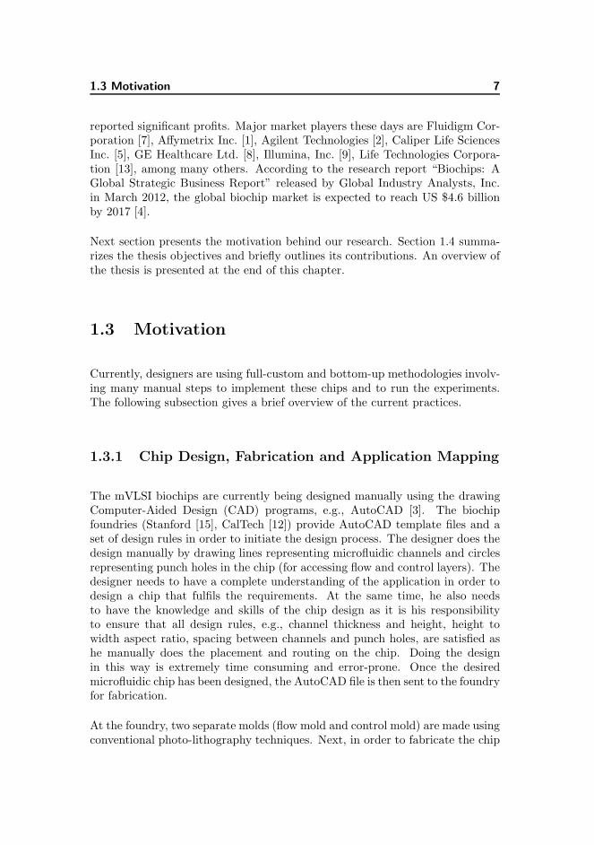
1.3 Motivation 7

reported significant profits. Major market players these days are Fluidigm Cor-poration [7], Affymetrix Inc. [1], Agilent Technologies [2], Caliper Life SciencesInc. [5], GE Healthcare Ltd. [8], Illumina, Inc. [9], Life Technologies Corpora-tion [13], among many others. According to the research report “Biochips: AGlobal Strategic Business Report” released by Global Industry Analysts, Inc.in March 2012, the global biochip market is expected to reach US $4.6 billionby 2017 [4].

Next section presents the motivation behind our research. Section 1.4 summa-rizes the thesis objectives and briefly outlines its contributions. An overview ofthe thesis is presented at the end of this chapter.

1.3 Motivation

Currently, designers are using full-custom and bottom-up methodologies involv-ing many manual steps to implement these chips and to run the experiments.The following subsection gives a brief overview of the current practices.

1.3.1 Chip Design, Fabrication and Application Mapping

The mVLSI biochips are currently being designed manually using the drawingComputer-Aided Design (CAD) programs, e.g., AutoCAD [3]. The biochipfoundries (Stanford [15], CalTech [12]) provide AutoCAD template files and aset of design rules in order to initiate the design process. The designer does thedesign manually by drawing lines representing microfluidic channels and circlesrepresenting punch holes in the chip (for accessing flow and control layers). Thedesigner needs to have a complete understanding of the application in order todesign a chip that fulfils the requirements. At the same time, he also needsto have the knowledge and skills of the chip design as it is his responsibilityto ensure that all design rules, e.g., channel thickness and height, height towidth aspect ratio, spacing between channels and punch holes, are satisfied ashe manually does the placement and routing on the chip. Doing the designin this way is extremely time consuming and error-prone. Once the desiredmicrofluidic chip has been designed, the AutoCAD file is then sent to the foundryfor fabrication.

At the foundry, two separate molds (flow mold and control mold) are made usingconventional photo-lithography techniques. Next, in order to fabricate the chip

8 Introduction

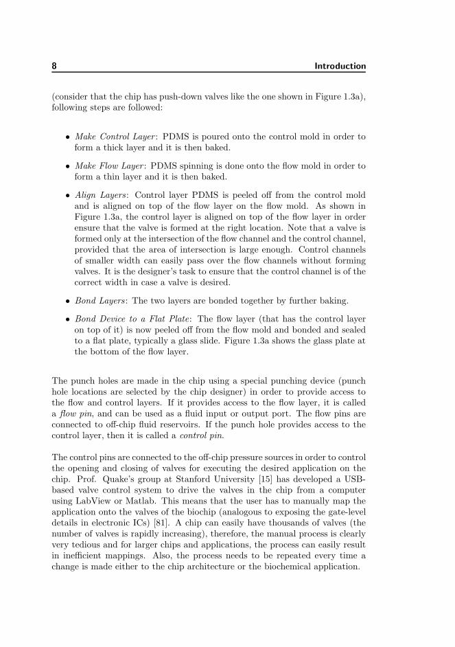
(consider that the chip has push-down valves like the one shown in Figure 1.3a),following steps are followed:

• Make Control Layer : PDMS is poured onto the control mold in order toform a thick layer and it is then baked.

• Make Flow Layer : PDMS spinning is done onto the flow mold in order toform a thin layer and it is then baked.

• Align Layers : Control layer PDMS is peeled off from the control moldand is aligned on top of the flow layer on the flow mold. As shown inFigure 1.3a, the control layer is aligned on top of the flow layer in orderensure that the valve is formed at the right location. Note that a valve isformed only at the intersection of the flow channel and the control channel,provided that the area of intersection is large enough. Control channelsof smaller width can easily pass over the flow channels without formingvalves. It is the designer’s task to ensure that the control channel is of thecorrect width in case a valve is desired.

• Bond Layers : The two layers are bonded together by further baking.

• Bond Device to a Flat Plate: The flow layer (that has the control layeron top of it) is now peeled off from the flow mold and bonded and sealedto a flat plate, typically a glass slide. Figure 1.3a shows the glass plate atthe bottom of the flow layer.

The punch holes are made in the chip using a special punching device (punchhole locations are selected by the chip designer) in order to provide access tothe flow and control layers. If it provides access to the flow layer, it is calleda flow pin, and can be used as a fluid input or output port. The flow pins areconnected to off-chip fluid reservoirs. If the punch hole provides access to thecontrol layer, then it is called a control pin.

The control pins are connected to the off-chip pressure sources in order to controlthe opening and closing of valves for executing the desired application on thechip. Prof. Quake’s group at Stanford University [15] has developed a USB-based valve control system to drive the valves in the chip from a computerusing LabView or Matlab. This means that the user has to manually map theapplication onto the valves of the biochip (analogous to exposing the gate-leveldetails in electronic ICs) [81]. A chip can easily have thousands of valves (thenumber of valves is rapidly increasing), therefore, the manual process is clearlyvery tedious and for larger chips and applications, the process can easily resultin inefficient mappings. Also, the process needs to be repeated every time achange is made either to the chip architecture or the biochemical application.

1.3 Motivation 9

As the chips grow more complex (commercial biochips are available which usemore than 25,000 valves and about a million features to run 9,216 polymerasechain reactions in parallel [66]) and the need of having multiple and concurrentassays on the chip becomes more significant, these manual, bottom-up method-ologies become highly inadequate. Therefore, new top-down design methodolo-gies and design tools are needed in order to successfully manage the increasein design complexity. The electronic VLSI circuits have benefited heavily fromdesign automation and the electronic designers today work as conveniently onthe billion transistor multi-core processors as they did on the Intel 4004 proces-sor with only 2,250 transistors in the early days. The CAD support for mVLSIbiochips is expected to enable the emergence of a large biochip market.

1.3.2 Related Work

In academia, significant amount of work has been carried out on the individualmicrofluidic components [49, 54]. The manufacturing technology, soft lithog-raphy, used for the flow-based biochips has advanced faster than Moore’s law[39]. Although biochips are becoming more complex everyday, Computer-AidedDesign (CAD) tools for these chips are still in their infancy. Most CAD researchhas been focussed on device-level physical modeling of components [43, 73].

Significant work on top-down synthesis methodologies for droplet-based biochipshas been proposed [24, 68]. However, the architecture of the droplet-basedchips differs significantly from the flow-based chips. In the flow-based biochips,components of different types (e.g., mixers, heaters) are physically designedon the chip and connected to each other using microfluidic channels. Oncefabricated, the number and type of the components, their placement schemeon the chip and the routing interconnections cannot be modified [55]. Droplet-based biochips (as discussed in Section 1.1), however, use the idea of virtualcomponents and are reconfigurable. Because of the architectural differences,the models and techniques proposed for the digital biochips are not applicableto their flow-based counterparts.

The industry has gotten around the limited CAD tools problem by limitingthe number of chips that they design and using them for multiple applications(Fluidigm Corporation has only 4 chip designs [6]). The soft lithography basedfabrication process is, however, cheap and has a fast turn around time [55],pointing to having application-specific chips capable of providing higher effi-ciency instead of doing a multi-purpose design.

Figure 1.5 shows the typical electronic VLSI and mVLSI design cycles. Giventhe system specifications (e.g., application requirements, chip area), the mVLSI

10 Introduction

Figure 1.5: VLSI vs mVLSI Design Cycles

design starts by designing the schematic of the required biochip. This is fol-lowed by the physical synthesis of the flow layer, i.e., placement of componentsand routing of flow channels while following the design rules. After the flowchannels have been routed, the channel lengths and therefore the routing la-tencies for the fluids that traverse these channels can now be calculated. Next,the given biochemical application is mapped onto this biochip architecture andthe optimized schedule for its execution is generated. Based on the schedule,the control information (which valves to open and close at what time and forhow long) can now be extracted. Optimization schemes can be used to sharecontrol pins between valves reducing the macro-assembly around the chip. Sincethe number of control pins and their sharing between valves is now known, thecontrol layer can now be routed. Once the routing is complete, the chip designis ready to be sent for fabrication.

The details of the related work, with respect to each of the design tasks describedabove, are discussed in the respective chapters.

1.4 Thesis Objectives and Contributions 11

1.4 Thesis Objectives and Contributions

In order to obtain a scalable, top-down approach for the design of mVLSIbiochips, the foremost step is to devise models for the biochip components,the biochip architecture as well as the biochemical applications that need to beexecuted on the chip. These models should be such that the design problems ofsynthesizing the biochip architectures, mapping of the biochemical applicationsto the mVLSI biochips and synthesizing the control for automatically executingthe application on the designed biochip can be easily formulated. These modelsand the design problem formulations are the primary contribution of this thesis.

Figure 1.6 shows our proposed design methodology. Our contributions are brieflyoutlined below:

• Modeling and Simulation

We propose a dual-layer modeling framework for the mVLSI components.The model captures the component operations at the flow layer as wellas the control layer valve activations that are needed in order to executethese operations [59, 58] (the box “Component Library” in Figure 1.6).We propose a topology graph-based model for the mVLSI biochips thatcaptures the chip components, their interconnections, the fluid flow pathson the chip and also the routing constraints. These models are used inall phases of the design methodology in Figure 1.6. For the biochemicalapplications we use a sequencing graph model (similar to the one used in

Figure 1.6: Design Methodology

12 Introduction

the digital biochips [78]), see box “Biochemical Application Model” inFigure 1.6. We have also developed simulators and editors based on thesemodels [62, 70].

• Application Mapping

Using our proposed models, we address the problem of mapping the bio-chemical application onto the mVLSI biochip [59, 58], see box “ApplicationMapping” in Figure 1.6. We propose a constraint programming (CP) [45]framework which, given a biochemical application and a biochip architec-ture, determines an optimal solution (in terms of application completiontime) for the binding and scheduling of the biochemical operations ontothe given biochip, without considering routing. We also propose a bind-ing and scheduling heuristic that takes the fluidic routing and channelcontention into account, while aiming to generate an optimized mapping.To the best of our knowledge, this is the first time that an applicationmapping framework is being proposed for the mVLSI biochips.

• Architectural Synthesis

We propose a top-down architectural synthesis methodology for the mVLSImicrofluidic biochips [61, 57]. Given a biochemical application, a microflu-idic component library and the chip area, the architectural synthesis (asshown in Figure 1.6) consists of the following three steps: (i) allocation ofcomponents from a given library, and performing the schematic design inorder to generate the netlist, the biochip (ii) flow layer physical synthesis,i.e., deciding the placement of the microfluidic components on the chipand performing routing of the microfluidic flow channels on the availablerouting layers creating component interconnections and the (iii) controllayer physical synthesis, i.e., deciding the placement of control pins androuting the control channels in order to connect the valves to the con-trol pins. To the best of our knowledge, this is the first time that thearchitectural synthesis framework for these chips is being proposed.

• Control Synthesis

We propose a top-down control synthesis framework for implementing bio-chemical applications on mVLSI biochips [65, 64]. As shown in Figure 1.6,given a biochip architecture and the mapping implementation of a bio-chemical application on the biochip architecture, control synthesis consistsof the following two steps: (i) control logic generation and, (ii) control pincount minimization. Control logic generation means determining whichvalves need to be opened or closed, in what sequence and for how long,in order to execute the application on the chip. We utilize the outputof control logic generation step and perform the control pin count mini-mization by sharing the control pins between multiple valves. To the best

1.5 Thesis Overview 13

of our knowledge, this is the first time an approach for the control logicgeneration for the mVLSI biochips is being proposed.

Different objective functions can be used for these design tasks. Minimizingthe application completion time is a useful objective function since it minimizesthe effects of environmental variations on the executing application and is alsodirectly relevant for the clinical diagnostics and environmental monitoring ap-plications. Minimizing the chip design area (e.g., to fit it under a microscope)or to minimize the number of control pins (to minimize the macro-assemblysurrounding the chip) are also realistic objective functions. Each chapter in thethesis mentions its targeted objective function.

In addition to the above mentioned design tasks, we also address the problemof maximizing the throughput of cell culture microfluidic biochips [63]. Thesechips can simultaneously perform multiple experiments and their throughput isdefined as the number of non-repeating experiments performed on the chip. Wepropose a strategy to maximize the number of experiments, saving cost both interms of time and money (the cell culture experiments are extremely expensiveto perform and it takes many days to complete one experiment).

The modeling and synthesis approach proposed is aimed at facilitating pro-grammability and automation, reducing human effort and minimizing the designcycle time. The target is also to decouple the development of complex bioassaysfrom the chip design and implementation process, allowing users to focus onapplications. The automated design flow is expected to be an enabler for thebiochip domain in the same manner as it has been for the electronic ICs in thelast three decades.

1.5 Thesis Overview

The thesis is organized in seven chapters. A brief summary of these chapters isas follows:

Chapter 2 presents the details of the proposed models. It starts off by pre-senting some basic concepts related to the mVLSI biochip architecture, followedup by the details of the proposed component and architecture models. Theapplication model used is also introduced in this chapter.

Chapter 3 describes the application mapping problem. It discusses the pre-vious state-of-the-art and our contribution to this design task. A constraintprogramming-based optimal solution approach as well as a List Scheduling-based

14 Introduction

binding and scheduling heuristic are described here in detail. The proposed al-gorithms are evaluated and the results are presented.

Chapter 4 provides the details of the mVLSI architectural synthesis problem.The problem is formulated after discussing the prior work at the start of thechapter. All the design tasks are explained in detail and then our synthesisstrategy is presented. The synthesis process involves component allocation,design schematic generation, and the physical synthesis (placement and routing)of the chip. The proposed strategy is experimentally evaluated using real-life aswell as synthetic benchmarks.

Chapter 5 presents the control synthesis problem in detail. Previous researchis discussed at the start followed by the problem formulation. Our algorithmgenerates the control logic needed to execute the application and uses a TabuSearch-based optimization in order to minimize the control pin count. Theapproach is evaluated and the results are presented.

Chapter 6 is dedicated to the cell culture microfluidic biochips. It starts byexplaining the architecture of the cell culture biochips and our modeling frame-work. The problem of throughput maximization for cell culture biochips is for-mulated using a detailed motivational example. This is followed by a discussionof our proposed solution strategy and the experimental evaluation.

The thesis is summed up by presenting the conclusions and the future workoptions in Chapter 7.

Chapter 2

System Model

We propose a topology graph-based system-level model of a biochip architecture,that is independent of the underlying biochip implementation technology. Wealso propose a dual-layer component model and have created a microfluidiccomponent library.

2.1 Biochip Architecture Model

Figure 2.1a shows the schematic view of a flow-based biochip with 4 input portsand 3 output ports, 1 mixer, 1 filter, 1 detector and 8 control pins (shown in red).Figure 2.1b shows the functional view of the same chip. All fluid samples insidethe chip occupy a fixed unit length (or a multiple of it) on the flow channel, i.e.,the fluid samples have discretized volumes. Unit length samples are obtained bya process called metering, carried out by transporting the sample between twovalves that are a fixed length apart [85]. In general, the chip is filled with a fillerfluid (e.g., immiscible oil) and the fluid samples are emulsified in the filler fluid.As emulsions, the samples do not touch the channel walls directly (preventingcross-contamination) and can be moved over long channel lengths of any shapewhile retaining their content [85].

16 System Model

(a) Biochip: Schematic View (b) Biochip: Functional View

Figure 2.1: Flow-Based Biochip Architecture

In order to make a fluid sample flow on the chip (e.g., Filter to the Mixer inFigure 2.1a):

• The point of fluid sample origin (Filter) needs to be connected to a pump(on-chip or off-chip) for generating the flow. All chip input ports aregenerally equipped with an off-chip pump and the filler fluid reservoirs.As shown in Figure 2.1a, the closest pump from the Filter is the off-chippump connected to the input port In1. We term the flow starting pointas the source (In1 in this case).

• The fluid sample destination point (Mixer) needs to be connected to afluidic output port (sink, e.g., Out1).

• A path for the fluid flow needs to be established from the source to thesink using the microfluidic valves.

• The desired flow (Filter to Mixer) can then be achieved by activatingthe pump.

For the Filter to Mixer flow in Figure 2.1a, the path is established by closingthe valve set v1, v3, v6 and v7, while the valve set v2, v4, v5 and v8 is kept open(the path is shown in black in Figure 2.1a). The entire path already containsthe filler fluid and the sample emulsified in the filler fluid is now present insidethe Filter. A pumping action at the source (In1) then creates a filler fluidflow towards the sink (Out1). The emulsified sample flows with the filler fluidfrom the Filter towards the Mixer. The pumping action is stopped once the

2.1 Biochip Architecture Model 17

Figure 2.2: Microfluidic Mixer

fluid sample reaches its destination (the green path in Figure 2.1a shows theflow of the sample). While the sample flows from the Filter to the Mixer, theestablished path (including the source, sink points) is reserved and cannot beused for any other flows.

2.1.1 Component Model

Consider the pneumatic mixer [25] in Figure 2.2a which is implemented usingnine microfluidic valves, v1 to v9. Figure 2.2b shows the conceptual view of thesame mixer. The valve set v4, v5, v6 acts as an on-chip pump. The valve setv1, v2, v3 is termed as switch S1 and the valve set v7, v8, v9 as switch S2.The two switches facilitate the inputs and outputs, and the pump is used toperform the mixing. The mixer output can either be sent to the waste or to theother components in the chip using the switch S3, as shown in Figure 2.2a.

The mixer has five operational phases. The first two phases represent the inputof two fluid samples that need to be mixed, followed by the mixing phase. The

18 System Model

mixed sample is then transported out of the mixer in the last two phases. Forthe first fluidic input (phase Ip1, depicted in Figure 2.2a), valves v1, v2, v7 andv8 are opened (together with v4, v5, v6), the pump at the Input is activated andthe liquid fills in the upper half of the mixer.

Note that the fluid samples that are to be mixed do not need to occupy thefull channel length from the Input to the upper half of the mixer. Rathereach sample occupies a certain length on the flow channel. As described inthe previous section, the process of measuring the length of each fluid sampleis called metering and is carried out by transporting the sample between twovalves that are a fixed length apart [85].

In Figure 2.2a, the mixer output is connected to a waste outlet making a closedloop (for the filler fluid to flow in) from the input to the waste outlet. The fillerfluid flows in from the input, goes through the mixer and into the waste outlet.The emulsified sample flows with the filler fluid and reaches the mixer. Oncethe top half is filled, the valves v7 and v2 close, stopping the filler fluid flow andblocking the fluid sample in the upper half of the mixer. Since we know theflow rate (mm/s) and the sample volume (in mm, measured in terms of lengththrough metering), the time until the mixer gets filled can be easily calculated.Therefore, an optical feedback is not necessary in order to activate the valves.

In the next phase Ip2, the second fluid sample fills the lower half of the mixer(Figure 2.2c(i)). Once both halves are filled, the mixer input and output valves(v1 and v8) are closed while valves v2, v3, v7, v9 are opened and the mixingoperation is initiated (Figure 2.2c(ii)). Valve set v4, v5, v6 acts as a peristalticpump. Closing valve v4 inserts some pressure on the fluid inside the mixer,closing valve v5 creates further pressure, then as valve v6 is closed valve v4 isopened again. This forces the liquid to rotate clockwise in the mixer. The valvesare closed and opened in a sequence such that the liquid rotates at a certainspeed accomplishing the mixing operation. Next, in phase Op1 (Figure 2.2c(iii)),half of the mixed sample is pushed out of the mixer towards the rest of the chipand in Op2 (Figure 2.2c(iv)), the other half is transported to the waste.

Using pressurized microfluidic valves in the control layer is the most commonlyutilized control method for the flow-based biochips. However, microfluidic com-ponents equipped with alternate control techniques (e.g., electro-osmotic, elec-trokinetic) have also been developed [49]. In order to have a unified designmethodology covering several underlying technologies, it is imperative to modelthe component implementation technology details separately from its opera-tional capabilities.

We propose a dual-layer component modeling framework, consisting of a flowlayer model and a control layer model. The flow layer model (P , C,H) of each

2.1 Biochip Architecture Model 19

Table 2.1: Mixer: Control Layer ModelPhase v1 v2 v3 v4 v5 v6 v7 v8 v91. Ip1 0 0 1 0 0 0 0 0 12. Ip2 0 1 0 0 0 0 1 0 03. Mix 1 0 0 Mix Mix Mix 0 1 04. Op1 0 0 1 0 0 0 0 0 15. Op2 0 1 0 0 0 0 1 0 0

component M is characterized by a set of operational phases P , execution timeC and the component geometrical dimensions H . The control layer model cap-tures the valve actuation details required for the on-chip execution of all op-erational phases of a component. For example, Table 2.1 presents the controllayer model of a pneumatic mixer, as presented in Figure 2.2, whose flow layermodel is characterized by the first row in Table 2.2. In Table 2.1, the valve ac-tivation for each phase is shown, ‘0’ representing an open and ‘1’ a closed valve.The status ‘Mix’ shown for the valve set v4, v5, v6 on line 4 of Table 2.1represents the mixing step in which these valves are opened and closed in aspecific sequence to achieve mixing. Microfluidic platforms are equipped with acontroller that manages all on-chip control, i.e., issuing signals to on-chip com-ponents for executing a biochemical application, performing data acquisitionand signal processing operations [49]. The control layer model of a componentcontains all the details required by the biochip controller.

Table 2.2 shows the component model library L = M(P , C. H) of eight com-monly utilized microfluidic components [49, 21]. The geometrical dimensionsH are given as length×width and are scaled, with a unit length being equalto 150µm, i.e., a length of 10 in Table 2.2 corresponds to 1500µm. Storageunit dimensions are for a storage with 8 reservoir channels and the multiplexerdimensions are for a 1-to-8 or 8-to-1 multiplexer. Multiplexers and their usageis discussed in detail in Chapter 6. The different operational phases listed fora component may or may not be executable in parallel depending on how thecomponent is implemented, e.g., the mixer presented here has only one inputport to receive both the input fluids, thus only one input phase can be activatedat a time.

2.1.2 Architecture Model

The research carried out for modeling the microfluidic architecture has beenfocused on the device-level physical models [43, 73]. We propose a system-levelmodel based on a topology graph in order to capture the biochip architecture.

20 System Model

Table 2.2: Component Library (L): Flow Layer ModelExec.

Component Phases (P ) Time (C) HMixer Ip1/ Ip2/ Mix/ Op1/ Op2 0.5 s 30×30Filter Ip/ Filter/ Op1/ Op2 20 s 120×30

Detector Ip/ Detect/ op 5 s 20×20Separator Ip1/ Ip2/ Separate/ Op1/ Op2 140 s 70×20Heater Ip/ Heat/ Op 20C/s 40×15

Metering Ip/ Met/ Op1/ Op2 - 30×15Multiplexer Ip or Op - 30×10Storage Ip or Op - 90×30

Figure 2.3: Biochip Architecture

Consider the biochip architecture shown in Figure 2.3. The chip has two in-puts, two outputs and is equipped with three mixers, one heater, one filter andeight storage reservoirs, i.e., the component ‘Storage-8’ contains eight reservoirs,Res1–Res8. The biochip architecture is modeled as a topology graph A = (N ,S, D, F , K, c), where N is a finite set of vertices, S is a subset of N , S ⊆ N , Dis a finite set of directed edges, F is a finite set of flow paths and K is a finite setof routing constraints. A vertex N ∈ N has two distinguished types: a vertexS ∈ S represents a switch (e.g., S1 in Figure 2.3), whereas a vertex M ∈ N ,/∈ S, represents a component or an input/output node (e.g., Mixer1 and In1,respectively, in Figure 2.3). A directed edge Di,j ∈ D represents a directed com-munication channel from the vertex Ni to vertex Nj , with Ni, Nj ∈ N (e.g.,DIn1,S1

represents a directed link from vertex In1 to vertex S1). A flow path, Fi

∈ F , is a subset of two or more directed edges of D, Fi ⊆ D, |Fi| > 1, represent-ing a directed communication link between any two vertices ∈ N using a chainof directed edges of D (e.g., FIn1,Mixer1 = (DIn1,S1

, DS1,Mixer1) represents a

2.1 Biochip Architecture Model 21

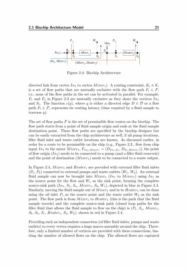
Figure 2.4: Biochip Architecture

directed link from vertex In1 to vertexMixer1). A routing constraint, Ki ∈ K,is a set of flow paths that are mutually exclusive with the flow path Fi ∈ F ,i.e., none of the flow paths in the set can be activated in parallel. For example,F1 and F3 in Figure 2.3 are mutually exclusive as they share the vertices In1

and S1. The function c(y), where y is either a directed edge D ∈ D or a flowpath Fi ∈ F , represents its routing latency (time required by a fluid sample totraverse y).

The set of flow paths F is the set of permissible flow routes on the biochip. Theflow path starts from a point of fluid sample origin and ends at the fluid sampledestination point. These flow paths are specified by the biochip designer butcan be easily extracted from the chip architecture as well, if all pump locations,filler fluid inlet and waste outlet locations are known. As discussed earlier, inorder for a route to be permissible on the chip (e.g., Figure 2.3., flow from chipinput In1 to the mixerMixer1, FIn1,Mixer1 = (DIn1,S1

, DS1,Mixer1)), the pointof flow origin (In1) needs to be connected to a pump (and a filler fluid reservoir)and the point of destination (Mixer1) needs to be connected to a waste output.

In Figure 2.4, Mixer1 and Heater1 are provided with external filler fluid inlets(P1, P2) connected to external pumps and waste outlets (W1, W2). An externalfluid sample can now be brought into Mixer1 (In1 to Mixer1) using In1 asthe source point for the flow and W1 as the sink point, forming the completesource-sink path (In1, S1, Sa, Mixer1, Sb, W1), depicted in blue in Figure 2.4.Similarly, moving the fluid sample out ofMixer1 and in to Heater1 can be doneusing the oil inlet P1 as the source point and the waste outlet W2 as the sinkpoint. The flow path is from Mixer1 to Heater1 (this is the path that the fluidsample travels) and the complete source-sink path (closed loop paths for thefiller fluid that allows the fluid sample to flow on the chip) is (P1, Sa, Mixer1,Sb, S5, Sc, Heater1, Sd, W2), shown in red in Figure 2.4.

Providing such an independent connection (of filler fluid inlets, pumps and wasteoutlets) to every vertex requires a huge macro-assembly around the chip. There-fore, only a limited number of vertices are provided with these connections, lim-iting the number of allowed flows on the chip. The allowed flows are captured

22 System Model

Table 2.3: Flow Path Set (F)F1 = (In1, S1, Mixer1), 2 sF2 = (In1, S1, S2, Mixer2), 2.5 sF3 = (In1, S1, S2, S3, Mixer3), 3 sF4 = (In2, S4, S3, S2, S1, Mixer1), 3.5 sF5 = (In2, S4, S3, S2, Mixer2), 3 sF6 = (In2, S4, S3, Mixer3), 2.5 sF7−x = (In1, S1, S2, S3, S4, Storage-8), 3.5 sF8−x = (In2, S4, Storage-8), 2 sF9 = (Mixer1, S5, Out2), 2 sF10 = (Mixer1, S5, Heater1), 2 sF11 = (Mixer1, S5, S6, S7, Filter1), 3 sF12−x = (Mixer1, S5, S6, S7, S8, Storage-8), 3.5 sF13 = (Mixer1, S5, S6, S7, S8, S10, Out1), 4 sF14 = (Mixer2, S6, S5, Out2), 2.5 sF15 = (Mixer2, S6, S5, Heater1), 2.5 sF16 = (Mixer2, S6, S7, Filter1), 2.5 sF17−x = (Mixer2, S6, S7, S8, Storage-8), 3 sF18 = (Mixer2, S6, S7, S8, S10, Out1), 3.5 sF19 = (Mixer3, S7, S6, S5, Out2, 3 sF20 = (Mixer3, S7, S6, S5, Heater1), 3 sF21 = (Mixer3, S7, Filter1), 2 sF22−x = (Mixer3, S7, S8, Storage-8), 2.5 sF23 = (Mixer3, S7, S8, S10, Out1), 3 sF24−x = (Storage-8, S4, S3, S2, S1, Mixer1), 3.5 sF25−x = (Storage-8, S4, S3, S2, Mixer2, 3 sF26−x = (Storage-8, S4, S3, Mixer3), 2.5 sF27−x = (Storage-8, S8, S7, S6, S5, Heater1), 3.5 sF28−x = (Storage-8, S8, S7, Filter1), 2.5 sF29−x = (Storage-8, S8, S10, Out1), 2.5 sF30−x = (Heater1, S9, S10, S8, Storage-8), 3 sF31 = (Heater1, S9, S10, Out1), 2.5 sF32−x = (Filter1, S9, S10, S8, Storage-8), 3 sF33 = (Filter1, S9, S10, Out1), 2.5 s

by the set of flow paths F . Table 2.3 shows a possible flow path set (permissibleroute set), F , for the biochip given in Figure 2.3. A shorter representation (us-ing the vertices traversed in the flow path) is chosen for clarity, for example, theflow path FIn1,Mixer1 = (DIn1,S1

, DS1,Mixer1) is represented as F1 = (In1, S1,Mixer1). Also, note that each flow path involving the storage reservoir (e.g.,F7−x) represents a set of eight flow paths (F7−1 to F7−8), i.e., one for each ofthe eight storage reservoirs. Each route (flow path) has an associated control

2.1 Biochip Architecture Model 23

layer model that contains the details required for its utilization, i.e., the switchsequence and the pump activation details.

The fluid transport latencies, c(F ), associated with each flow path are also listedin Table 2.3. For calculating the latencies, we abstract away from absolutefluid volumes and utilize the concept of a unit fluid volume instead (capturedby metering as explained in Section 2.1.1). Each fluidic I/O (input/outputphase of a component) is characterized by a volume weight wv, which is usedto calculate the transport latency of a certain flow path when utilized for thatspecific fluidic I/O. Similarly, each component also has an associated capacityweight wc, representing its volume capacity. For this example, we assume avolume weight of one for all fluidic I/Os. The capacity weight of all microfluidiccomponents is assumed to be the same as its number of input phases, e.g., amixer has two input phases, therefore it has a capacity weight equal to two.Also, a fluid with volume weight one occupies a fixed channel length wl on thechip. In the thesis, we assume this channel length to be equal to 10 mm.

The latencies for the flow paths have been calculated using a typical flow rateof 10 mm/s [49] and the chip dimensions of 5 mm between any two networkvertices, Ni and Nj (termed as a segment), with Ni, Nj ∈ N . For example,F1 = (In1, S1,Mixer1) traverses two segments, i.e., In1 to S1 and S1 toMixer1,thus a total channel length of 10 mm. With a flow rate of 10 mm/s, a fluid withvolume weight one (occupying a total channel length of 10 mm) would have atotal latency of 2 seconds from the time the fluid tip enters from In1 till thefluid tail disappears into the mixer Mixer1.

Analogous to a circuit-switched network, when a flow path gets activated, theentire route (from the source to the sink) is reserved until the completion ofthe fluid transfer. This imposes routing constraints on the chip. All those flowpaths in the set F that have a network vertex Ni in common in their source-sink paths are considered as mutually exclusive, i.e., the routes represented bythese flow paths can only be utilized in a serialized fashion. For example inFigure 2.3, FIn1,Mixer1 and FIn1,Mixer2 are mutually exclusive as they share thevertices In1 and S1. The routing constraints associated with the flow path setin Table 2.3 are shown in Table 2.4. The first row in the routing constraints(K1 : (F2, F3, F4, F7, F24)) shows that F1 cannot be executed in parallel withF2, F3, F4, F7 and F24.

Since fluid samples are expendable and cannot be reused limitless number oftimes (unlike the operands in computers), the fluid volumes need to be managedinside the chip. Researchers have proposed methods for carefully distributing theliquid volume, preventing overflow and underflow of the fluid samples [20]. Weassume that the designer does this beforehand while designing the biochemicalapplication, ensuring that both overflow and underflow are avoided.

24 System Model

Table 2.4: Routing Constraints KK1 : (F2, F3, F4, F7, F24)K2 : (F1, F3, F4, F5, F7, F24, F25)K3 : (F1, F2, F4, F5, F6, F7, F24, F25, F26)K4 : (F1, F2, F3, F5, F6, F7, F8, F24, F25, F26)K5 : (F2, F3, F4, F6, F7, F8, F24, F25, F26, F27)K6 : (F3, F4, F5, F7, F8, F24, F25, F26)K7−x : (F1, F2, F3, F4, F5, F6, F8 , F24, F25, F26)...K33 : (F13, F18, F23, F29, F30, F31, F32)

2.2 Biochemical Application Model

Biochemical applications have traditionally been described through a sequenceof steps given in free-flowing English-language text. Such descriptions are oftenambiguous and incomplete and are not adequate for automation of biochemicalprotocols. Researchers have proposed standardizing programming languages inorder to express biochemical applications [22].

We model a biochemical application using a sequencing graph [88]. Real-lifeassays can be converted to this model using [22]. The graph G(O, E) is directed,acyclic and polar (i.e., there is a source vertex that has no predecessors and asink vertex that has no successors). Each vertex Oi ∈ O represents an opera-tion that can be bound to a component using a binding function B : O → M.

Each vertex has an associated weight CMj

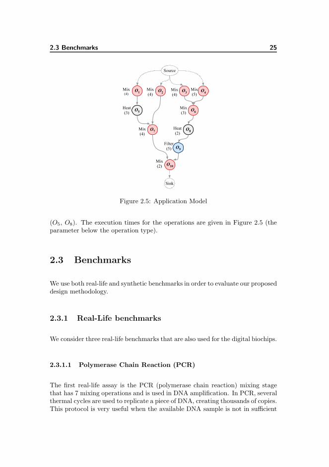
i , which denotes the execution timerequired for the operation Oi to be completed on componentMj . The executiontimes provided in Table 2.2 are of the actual functional phase (given in bold inthe table, e.g., Mix). These execution times are taken as the typical executiontimes for the said component types, i.e., typical mixing time is 0.5 s but a bio-chemical application description may specify a longer time (e.g., 5 s) if requiredfor a particular operation. This value does not include the time required tofetch the input fluids or to remove the output fluids from the component. Theinput/output (I/O) phases are dependent on the chip architecture and are thuscaptured by the set of flow paths F in the biochip architecture model A. Theedge set E models the dependency constraints in the assay, i.e., an edge ei,j ∈ Efrom Oi to Oj indicates that the output of Oi is the input of Oj . All inputs needto arrive before an operation can be activated. We assume that the biochem-ical application has been correctly designed, such that all operations will havethe correct volume of liquid available for their execution. Figure 2.5 shows anexample of a biochemical application model which has seven mixing operations(O1–O4, O6, O7, O10), one filtration operation (O9) and two heating operations

2.3 Benchmarks 25

Figure 2.5: Application Model

(O5, O8). The execution times for the operations are given in Figure 2.5 (theparameter below the operation type).

2.3 Benchmarks

We use both real-life and synthetic benchmarks in order to evaluate our proposeddesign methodology.

2.3.1 Real-Life benchmarks

We consider three real-life benchmarks that are also used for the digital biochips.

2.3.1.1 Polymerase Chain Reaction (PCR)

The first real-life assay is the PCR (polymerase chain reaction) mixing stagethat has 7 mixing operations and is used in DNA amplification. In PCR, severalthermal cycles are used to replicate a piece of DNA, creating thousands of copies.This protocol is very useful when the available DNA sample is not in sufficient

26 System Model

Figure 2.6: Polymerase Chain Reaction (PCR)

enough quantity for performing the analysis. The first step of the polymerasechain reaction consists of seven mixing operations, denoted in Figure 2.6 byO1 to O7. The output of this stage undergoes a series of thermal cycles forperforming DNA amplification [44].

2.3.1.2 In-vitro Diagnostics (IVD)

Multiplexed IVD (in-vitro diagnostics) has a total of 12 operations. Figure 2.7describes the protocol for an in-vitro diagnostics assay (IVD) in which the level

Figure 2.7: In-Vitro Diagnostics (IVD)

2.3 Benchmarks 27

of different metabolites in human physiological fluids are measured. The assaysrequires the input of samples (urine, plasma, and serum), reagents (glucoseoxidase, lactate oxidase) and buffer substance. The level of glucose and oxidaseare measured for each type of physiological fluid using the detection operations.

2.3.1.3 Colorimetric Protein Assay (CPA)

The application graph in Figure 2.8 describes a protein assay which is used fordetermining the concentration of a certain protein in a solution. The procedurecauses a reaction between the protein of interest and a dye. The concentra-tion of the protein is determined by measuring the absorbance of a particularwavelength in the resulted substance. The protocol consists of 55 microfluidicoperations and uses three types of liquids: physiological fluid (sample contain-ing the protein), Coomassie Brilliant Blue G-250 dye as reagent and NaOH asbuffer substance. Before being mixed with the dye, the sample is first dilutedwith the NaOH buffer. Dilution is represented as mixing in the applicationgraph. The protocol finishes with detection operations, in which the proteinconcentration for the resultant solution is measured. The letter “S” in the ap-plication graph represents the Source, which means that the input comes fromthe off-chip reservoirs.

2.3.2 Synthetic benchmarks

We consider five different synthetic benchmarks. The benchmark applicationsare composed of 10, 20, 30, 40 and 50 operations. Figure 2.9 – 2.13 present thesynthetic benchmarks.

28 System Model

Figure 2.8: Colorimetric Protein Assay (CPA)

Figure 2.9: Synthetic Benchmark - 10 Operations

2.3 Benchmarks 29

Figure 2.10: Synthetic Benchmark - 20 Operations

Figure 2.11: Synthetic Benchmark - 30 Operations

30

System

Model

Figure 2.12: Synthetic Benchmark - 40 Operations

2.3

Benchmarks

31

Figure 2.13: Synthetic Benchmark - 50 Operations

32 System Model

2.4 Summary

In this chapter we have presented our proposed biochip architecture and com-ponent models. The model used for the biochemical application has also beenintroduced. We have also given the details of the benchmarks considered in thisthesis. Using these models, in the next chapter, we propose our approach formapping the biochemical applications onto the mVLSI biochips and evaluatethe approach using the mentioned benchmark applications.

Chapter 3

Application Mapping

The block diagram of our proposed design methodology is shown in Figure 1.6.In this chapter, we focus on the “Application Mapping” block. It takes thebiochemical application model and the models of the biochip architecture andthe biochip components as input. As output, it generates the implementationΨ < B,X > which contains the binding and scheduling details of the operationsas well as the fluid routing information.

3.1 Related Work

Currently, researchers manually map the applications to the valves of the chipusing some custom interface (analogous to exposure of gate-level details) [81].The manual process is quite tedious and needs to be repeated every time achange is made either to the chip architecture or the biochemical application.For larger chips and applications, the process can easily result in inefficientapplication mappings.

Researchers have proposed significant work on top-down synthesis techniquesfor droplet-based biochips [24]. However, as discussed in Chapter 1, these tech-niques are not applicable to the flow-based chips and, to the best of our knowl-

34 Application Mapping

edge, no automated application mapping approach has been proposed so far forthe flow-based biochips.

3.2 Contribution

Using the models proposed in the previous chapter, we focus on the problem ofmapping a biochemical application, modeled as a sequencing graph (capturingthe operations and their dependency constraints), onto a given biochip architec-ture. We propose a constraint programming (CP) [45] framework which, givena biochemical application and a biochip architecture, determines an optimalsolution (in terms of application completion time) for the binding and schedul-ing of the biochemical operations onto the given biochip. CP makes it possibleto specify the resource and timing constraints, and to capture the applicationbinding and scheduling within the same framework. Using the CP formulation,a solver then searches for the optimal solution.

In microfluidic biochips, routing latencies are comparable to the operation execu-tion times, thus having a considerable influence on the schedule. The CP-basedsolutions, although optimal, require a large computation time when more com-plex chips are introduced and fluidic routing is included inside the implementa-tion. We propose a List Scheduling (LS)-based binding and scheduling heuristicthat also takes the fluidic routing and channel contention into account, whileaiming to generate an implementation that minimizes the application comple-tion time. The heuristic produces good quality solutions in small time. Weevaluate the proposed framework by synthesizing real-life case studies as well assynthetic benchmarks.

Next section discusses the design tasks involved in the biochip synthesis. Thetargeted problem is formulated at the end of this section. The proposed CP-based synthesis approach is presented in Section 3.4 and the LS-based approachin Section 3.5. We evaluate our framework in Section 3.6

3.3 Application Mapping

Mapping the application onto the architecture involves binding of operationsonto the allocated components, scheduling the operations and performing therequired fluidic routing. This section explains these design tasks using the bio-chemical application in Figure 3.1a and the biochip architecture given in Fig-ure 3.1b. The architecture is modeled as described in Section 2.1. Thus, the

3.3 Application Mapping 35

(a) Application Graph (b) Biochip Architecture

Figure 3.1: Illustrative Example

allocated components are captured by the vertex set M, M ∈ N , in the archi-tecture model A. Table 3.1 shows the set M for the biochip given in Figure 3.1b.The component placement and interconnections are also given, and are capturedby the remaining elements of the topology graph A modeling the architecture,as discussed in Section 2.1. Table 2.3 shows the flow path set (permissibleroute set), F , for the biochip given in Figure 3.1b. The routing constraints (asdiscussed in Section 2.1.2) extracted from the set are shown in Table 2.4.

Figure 3.2 shows the schedule for executing the biochemical application in Fig-ure 3.1a on the biochip architecture in Figure 3.1b. The schedule is representedas a Gantt chart, where, we represent the operations and fluid routing phases asrectangles, with their lengths corresponding to their execution duration. Eachoperation is placed in a separate row. During the binding step, each vertex Oi,Oi ∈ O, representing a biochemical operation in the application model in Fig-

Table 3.1: Allocated Components (M)Function Units NotationsInput port 2 In1, In2

Output port 2 Out1, Out2Mixer 3 Mixer1, Mixer2, Mixer3Heater 1 Heater1Filter 1 Filter1

Storage Reservoir 8 Res1–Res8

36 Application Mapping

Figure 3.2: Schedule

ure 3.1a is bound to an available componentMj , i.e., B(Oi) =Mj . For example,the mixing operation O1 in the application model in Figure 3.1a is bound tothe component Mixer1 as shown in Figure 3.2. Since the fluid transport laten-cies in microfluidic chips are comparable to the operation execution times, fluidrouting also needs to be considered during the synthesis phase. This means thatthe binding function must also capture the binding of the edge set E ∈ G to anavailable route. The available route can be a flow path, F ∈ F , or a collectionof flow paths called a composite route. A composite route is used if the sourceand destination components are such that no direct flow path exists betweenthem.

A scheduling strategy is needed to efficiently execute the biochemical operationson the chip components, while considering the dependency and resource con-straints captured by the biochemical application and the biochip architecturemodels, respectively. In Figure 3.2, operation O6 bound to Mixer2 starts im-mediately after all its predecessors (O3, O4) are complete and the input fluidshave been routed to Mixer2. It starts at t

startO6

= 20.5 s and takes 3 s, finishing

at time tfinishO6= 23.5 s.

Together with the set of operations O ∈ G given in the application model, theedge set E ∈ G also needs to be scheduled on the chip, while taking the rout-ing constraints into account. Before scheduling the edge, the implementationneeds to evaluate if a flow path F ∈ F is sufficient to bind the edge, or if acollection of flow paths (composite route) is needed. For example, the edge e6,8,modeling the transport of the output of O6(Mixer2) (operation O6 bound tocomponentMixer2) to O8(Heater1), can be directly bound to the flow path F15

(Table 2.3). The edge e5,7 models the output of O5(Heater1) being transportedto O7(Mixer3). However, there is no flow path F ∈ F that connects Heater1 to

3.4 Constraint Programming-Based Strategy 37

Mixer3. Therefore, a composite route (consisting of a collection of flow paths)needs to be generated. The edge e5,7 is bound to the composite route (F30−1,F26−1) as shown in Figure 3.2.

During the scheduling phase, the storage requirement analysis needs to be per-formed as well. This means that after completion of an operation, a decisionon whether the output fluid (analogous to the operand) should be moved to thestorage reservoir or not, needs to be made.

3.3.1 Problem Formulation

The problem addressed here can be formulated as follows: Given (1) a biochem-ical application modeled as a sequencing graph G, (2) a biochip architecturemodeled as a topology graph A, and (3) a characterized component library L,we are interested in synthesizing an implementation Ψ that minimizes the ap-plication completion time while satisfying the dependency, resource and routingconstraints. Synthesizing an implementation Ψ = < B, X > means deciding on(1) the binding B of each operation Oi ∈ O to a component Mj ∈ M, and eachedge ei,j ∈ E to a flow path Fi ∈ F (or to a composite flow path generated bythe implementation), and (2) the schedule X of the operations and the edges,which contains the start time tstart of each operation Oi and edge ei,j on itscorresponding component and (composite) flow path.

3.4 Constraint Programming-Based Strategy

The problem can be considered equivalent to the resource constrained schedulingproblem with non-uniform weights, which is NP-complete [83, 60]. CP offersvery good performance for such problems [45]. Typically, a problem defined inCP has three primary elements: (1) a set of variables capturing the system, (2) aset of finite domains of the values for these variables and (3) a set of constraintsimposed on these variables. The solution of such a problem is the assignmentof values to all variables from their respective domains such that all constraintsare satisfied. If an optimal solution is desired, then a cost function also needsto be defined in terms of the variables. The solver then tries to find the optimalsolution in terms of the cost function that satisfies all constraints.

Our CP-based implementation generates optimal solutions for the binding andscheduling of operations onto the biochip architecture. This approach ignoresthe fluidic routing, which we address in Section 3.5. Figure 3.3 shows the optimal

38 Application Mapping

schedule for executing the application in Figure 3.1a onto the architecture inFigure 3.1b. We have used the constraint programming environment Gecode[71] for our implementation.

3.4.1 Finite Domain Variables

We use the following primary finite domain variables (FDV) to model the bind-ing and scheduling of all biochemical operations:

• tstartOi:: 0..∞ defines the start time of operation Oi. For example, oper-

ation O5 in Figure 3.3 has the start time tstartO5= 4 s.

• Mi :: 0.. |M|−1 defines the resource (component) to which the operationOi is bound where |M| is the total number of components on the chip.For example, in Figure 3.3 |M| = 5. Each resource is assigned a uniquenumeric identifier (ID) and the range of the identifiers is 0.. |M|−1, i.e.,0..4 for the current example. For Figure 3.3, ID of Mixer1 is 0, Mixer2is 1, Mixer3 is 2, Heater1 is 3 and Filter1 is 4. So for operation O5,M5 = 3, which is the ID of Heater1.

• δG :: 0..∞ defines the cost function (application completion time). Ap-plication completion time is the end-to-end time taken by the applicationto complete its execution, i.e., from the start time of the first executedoperation to the finish time of the last executed operation. For examplein Figure 3.3, the application completion time is δG = 17 s, which is thefinish time of the last executed operation O10.

Figure 3.3: Optimal Schedule

3.4 Constraint Programming-Based Strategy 39

Secondary FDVs are introduced, where needed, in order to implement the con-straints.

3.4.2 Resource Binding Constraints

An operation can only be bound to a component which is capable of executingit, i.e., a mix operation must be bound to one of the mixers and not to any othercomponent, e.g., heaters. Based on the type of the operations, we constrain thedomain of the FDV Mi in order to exclude the forbidden components. Eachoperation is treated as a tuple (Oi, αi), where Oi ∈ O is an operation and αi

⊆ M is a set of available components capable of performing the operation. Abinding must respect,

Mi ∈ αi, ∀i ∈ 1.. |O| (3.1)

where |O| defines the total number of operations in the application graph G,e.g., application given in Figure 3.1a has 10 operations. For operation O1 (amix operation), α1 = 0, 1, 2 which represents the IDs of the three mixers.For O1 in Figure 3.3, M1 = 0 (ID for Mixer1) which is a member of the set α1,thus satisfying the resource binding constraint.

3.4.3 Resource Sharing Constraints

Operations bound to the same component (e.g., O3 and O6 are bound toMixer2in Figure 3.3) must not overlap in time. We use three disjunctive constraints inorder to implement this for all possible combinations of operations.

∀i, ∀(j > i)

(tstartOi+ Ci ≤ tstartOj

) ∨ (tstartOj+ Cj ≤ tstartOi

) ∨ (Mi 6=Mj),

∀(i, j) ∈ 1.. |O| (3.2)

where Ci represents the execution time of operation Oi. We consider two op-erations (Oi, Oj) at a time. At least, one of the three constraints given inthe above equation needs to be true in order to ensure that the resources arecorrectly shared.

The first constraint, (tstartOi+ Ci ≤ tstartOj

), means that the finish time of oper-ation Oi should be less than or equal to the start time of operation Oj . For

40 Application Mapping

example for (O1, O2) in Figure 3.3, the finish time for O1 (4 s) is equal to thestart time of O2, thus the constraint is satisfied. If the first constraint is notsatisfied (consider (O7, O2) in Figure 3.3, the finish time for O7 (12 s) is notless than or equal to the start time of O2 (4 s)), then the second constraint,(tstartOj

+ Cj ≤ tstartOi), is considered. For (O7, O2) in Figure 3.3, the finish time

for O2 (8 s) is equal to the start time of O7 (8 s), thus the constraint is satisfiedfor this pair of operations. The third constraint, Mi 6=Mj, is considered if boththe first and second constraint are not satisfied. Consider (O1, O3), the finishtime for O1 (4 s) is not less than or equal to the start time of O3 (0 s) and thefinish time for O3 (4 s) is also not less than or equal to the start time of O1 (0 s).In this case, the third constraint must be true. Here, M1 = 0 (Mixer1) andM3 = 1 (Mixer2), satisfying the resource sharing constraint.

3.4.4 Precedence Constraints

During scheduling, an operation must not start executing until its predecessorhas completed its execution, e.g., in Figure 3.1a, O6 must finish before O8 canstart. The following constraint is added for each required precedence:

tstartOi+ Ci ≤ tstartOj

(3.3)

where operation Oi is a predecessor of operation Oj .

3.4.5 Cost Function

We are interested in a solution that minimizes the application completion time(cost function δG). We constrain the cost function to be greater than or equalto the finish time of the operation Oi, i.e.,

tstartOi+ Ci ≤ δG , ∀i ∈ 1.. |O| (3.4)

minimize δG (3.5)

Minimization of the δG generates the optimal solution, which satisfies all theimposed constraints. In order to reduce the search space and speed up theresult generation, we place an upper and lower bound on δG . The upper boundis the sum of execution times of all operations as that is the largest possibleapplication completion time. For the example in Figure 3.1a, the upper boundis 36. The lower bound is equal to the duration of the critical path in the givenapplication graph G. Critical path is defined as the path in the application

3.5 List Scheduling-Based Strategy 41

graph, going from the source nodes to the sink nodes, that has the largestduration. For example in Figure 3.1a, the critical path consists of the nodesO4, O6, O8, O9, O10 and has the duration equal to 17 s. The lower boundvalue (lower bound) is provided as an input to our CP framework.

δG ≤∑

Ci, ∀i ∈ 1.. |O| (3.6)

δG ≥ lower bound (3.7)

3.5 List Scheduling-Based Strategy

The manufacturing technology for the flow-based chips has advanced fasterthan Moore’s law [39], resulting in ever increasing complexity for these chips.Although CP-based approach generates optimal solutions but as the problembecomes larger and more complex, the CP-based approach becomes computa-tionally too intensive.

We propose a heuristic approach to solve the problem in a computationally effi-cient manner. Together with the operation binding and scheduling, our heuristicapproach also considers the fluidic routing and channel contention.

The requirement of scheduling the routing together with the task operations,while satisfying the routing constraints, makes the problem analogous to thecommunication contention aware scheduling in parallel computing systems. Weutilize the well-known List Scheduling Algorithm (LS) [56] and extend it withcontention awareness [74] by also scheduling the edges (E in G) onto the com-munication channels during the synthesis process.

The schedule shown in Figure 3.2 has been generated using our LS-based synthe-sis algorithm shown in Figure 3.4. The operations of the biochemical applicationare topologically sorted based on the dependency constraints. At each controlstep, operations are evaluated and the ready ones are found (the operationswhose predecessor operations have been completed). Each new control stepmarks an operation event generation, with the operation event being defined asthe completion of a scheduled operation. The list of ready operations is prior-itized using the urgency criteria. The urgency of an operation is specified bythe length of the longest path from the operation to the sink, i.e., summing upthe execution weights of the vertices and the latency times for the edges. Anaverage latency of 3 s is considered per edge based on the biochip architecturegiven in Figure 3.1b. An average is used since it is unclear on which flow pathsthe edges would be bound, unless binding of all operations has been completed

42 Application Mapping

BiochipSynthesis(G, A, L)

1 Initialize < B, Bo, X > to φ2 while <all operations and edges are not scheduled> do3 // Phase I: Bind Operations and Edges4 while <all possible ready operations are not bound> do5 Bo = BindOperations(G, A)6 Bo = BindStorage(Bo, B, X )7 Bo = GenRouteAndBindEdges(Bo, A, L)8 end while9 B = Record(Bo)

10 // Phase II: Schedule Operations and Edges11 while <an operation event does not occur> do12 X = ScheduleOperationsAndEdges(B, X , A)13 Advance time to next event14 end while15 end while16 return Ψ = < B, X >

Figure 3.4: Synthesis Algorithm for Flow-Based Biochips

(defining the source and destination component for each edge). The urgencyvalue for O1 in Figure 3.1a is 25. If the number of ready operations exceedsthe number of available resources, the most urgent operations (having higherurgency value) are scheduled and the remaining ones are deferred.

We perform the implementation synthesis in two phases. In Phase-I, we startoff by binding the ready operations to the available resources (line 5). Thealgorithm tries all possible bindings and chooses the one that produces theshortest completion time for that operation. For example after control step 5,both Mixer1 and Mixer3 are available as the mixing operation O7 is released,i.e., both its predecessor operations O2 and O5 have been completed. As shownin Figure 3.2, O2 was bound to Mixer3 and its output is still inside the mixerunit when O7 is released (i.e., its output has not been moved to the storageunit). The algorithm binds O7 to Mixer3 preventing the routing delay thatwould have occurred had O7 been bound to Mixer1.

Next, we evaluate if a reservoir is required to store the output of the operationsthat finished in the previous control step (line 6) and if so, bind it to a particularreservoir. A storage reservoir is utilized only (1) if the component to which theprevious operation was bound is needed for performing another operation and(2) the successor of the previous operation is not scheduled during the currentcontrol step. For example in Figure 3.2, O4 (bound to Mixer3) was completedin control step 1. Its successor (O6) is not scheduled in control step 2 and

3.5 List Scheduling-Based Strategy 43

Mixer3 is needed to perform O2. Based on the above given criteria, output ofO4 is bound to the storage reservoir Res1 at the start of control step 2.

Next we generate the routes (single flow path or composite route) for performingthese operations and bind the edges to the generated routes (line 7). We startby fetching the phase information of the components (e.g., Mixer3 for O4) fromthe library L (Table 2.2) and bind the I/O phases (Ip1, Ip2, Op1, Op2) tothe corresponding generated routes (e.g., F3 for Ip1 of Mixer3). If a route isnot found, the operation is deferred. The algorithm jumps back to line 5 inorder to modify the binding for the current control step (Bo), by binding a lowpriority operation that was earlier deferred because of lack of resources. Oncethe binding has been finalized, it is recorded into the binding information B(line 9). More details about route generation are given in following subsection.

In Phase-II (lines 11–14), we generate the schedule for the operations and theedges bound in Phase-I. Starting from the input edges associated with the op-eration of the highest priority (based on the urgency criteria, O4 in this case),we start scheduling the edges one by one (here the first one is F3). In order toreduce the schedule length, we try to schedule as many bound edges as possiblein parallel. All the ready edges that do not violate the routing constraints (listedin Table 2.4 ) can be utilized in parallel. An edge is considered a ready edgeif it does not violate any inter- or intra-operation dependency constraints. Theinter-operation dependency constraints are given by the application model G(e.g., O3 and O4 need to complete before O6). The intra-operation dependencyconstraints means that the inputs of an operation and the operation itself needto be completed before its outputs can be issued (e.g., F3, F6 and the mixingoperation in Mixer3 need to complete before F22−1 and F19 can be scheduled).Multiple inputs/ outputs for the same operation (F3, F6 for Mixer3) are inde-pendent of each other and can be parallelized if the routing constraints permit.

Figure 3.5 shows the schedule for the first control step (Figure 3.2 shows thecomplete schedule). Since O4 (bound on Mixer3) has the highest priority, F3

is the first bound edge that is scheduled. None of the other edges (boundto flow paths) in the ready set < F6, F2, F5, F1, F4 > can be scheduled inparallel with F3 because of the routing constraints given in Table 2.4, thusF3 is scheduled alone as shown in Figure 3.5. Once all possible edges andoperations are scheduled (only F3 in this case), we advance time to the nextevent (operation event marking completion of an operation, or an edge eventrepresenting completion of an edge execution) (line 13). An operation eventtriggers a new control step and the algorithm switches back to Phase-I, whereasan edge event means that the next edge needs to be scheduled. Completion ofF3 thus triggers an edge event. We schedule F6 (next edge in the highest priorityoperation O4) and try to optimize the schedule again (F2 can be scheduled inparallel with F6). The operations are scheduled as soon as all their input edges

44 Application Mapping

Figure 3.5: Edge and Operation Events

have been executed (e.g., O4 after F3 and F6). When an operation finishes (e.g.,O4 onMixer3 in control step 1) it triggers an operation event and the algorithmjumps back to Phase-I.

The process is repeated until all operations/ edges are scheduled. The imple-mentation Ψ, consisting of binding B and scheduling X information, is thenreturned (line 16).

3.5.1 Route Generation

GenRouteAndBindEdges (line 7) is used to generate the fluid route from theselected source to the selected destination (e.g., from In1 to Mixer1). If a flowpath exists, then it binds the edge to that flow path and returns the bindinginformation. If the selected operation has the selected source and destinationsuch that no flow path exists to route the fluid from the source to the des-tination (e.g., Heater1 → Mixer3, control step 5–7 in Figure 3.2), then thealgorithm searches for a composite route, i.e., a route linking the desired sourceand destination using more than one flow path.

If multiple composite routes exist, the shortest one (in terms of cumulativelatencies) is selected. For (Heater1 → Mixer3), the composite route (Heater1→ Res1, Res1 → Mixer3) is selected. Note that this requires all intermediatedestinations (Res1 — reservoir 1 in the storage) to be available.

If no direct route is available and no composite route can be specified as well(e.g., intermediate destinations not available), then the operation is deferred.

3.6 Experimental Evaluation 45

Phase-I (lines 4–8) is repeated again to see if any of the other low priorityoperations (that were not scheduled earlier because of resource constraints) cannow be scheduled instead. Once all possible operations and edges are bound,the algorithm switches to Phase-II.

3.6 Experimental Evaluation

We evaluate our proposed CP- and LS-based approaches by synthesizing reallife assays as well as synthetic benchmarks onto different biochip architectures.The CP framework was implemented in Gecode constraint programming envi-ronment [71] and the LS-based algorithm was implemented in C++, running onLenovo T400s ThinkPad with Core 2 Duo Processors at 2.53 GHz and 4 GB ofRAM.

Table 3.2 shows our experimental results for the CP-based synthesis approach.Column 1 presents the application and column 2 shows the list of allocated com-ponents in the following format (Mixers, Heaters, Filters, Detectors). Column 3presents the optimal application completion time δG obtained using CP. Wecompare the results to our list scheduling based approach by ignoring the flu-idic routing in the LS-based approach as well. Column 4 shows the applicationcompletion time generated using the LS-based approach. Column 5 presents thetime taken by CP to generate the solution and column 6 gives the time takenby the LS-based approach.

The first real-life assay is the PCR (polymerase chain reaction) mixing stage.We synthesize the assay on three different biochip architectures varying thenumber of mixers. Each mixing operation is considered to have an executiontime of 4 s on the mixing units used in the biochips. As shown in Table 3.2,both CP and LS generate optimal solutions.

Next real-life assay is the multiplexed IVD (in-vitro diagnostics). As given inTable 3.2, IVD is synthesized onto three different biochip architectures. Eachmixing operation is considered to have an execution time of 4 s and the detectionoperation 7 s. Increasing the number of components reduces δG for IVD from25 s to 11 s.

The example application (EA) given in Figure 3.1a is used as a synthetic bench-mark. We vary the number of resources and generate optimal values of δG . TheCP framework facilitates design space exploration enabling biochip designers totake early design decisions. For example in Table 3.2, the result (row 8 androw 9) shows that increasing the number of mixers from 3 to 4 and the heaters

46 Application Mapping

Table 3.2: Experimental Results: CP-Based Synthesis

Appl. Allocated δG−CP δG−LS CP Exec. LS Exec.Components Time Time

(2, 0, 0, 0) 16 s 16 s 0.2 s < 0.1 sPCR (3, 0, 0, 0) 16 s 16 s 0.2 s < 0.1 s

(4, 0, 0, 0) 12 s 12 s 0.2 s < 0.1 s

(2, 0, 0, 2) 25 s 25 s 2.6 < 0.1 sIVD (5, 0, 0, 5) 18 s 18 s 38 min 28 s < 0.1 s

(6, 0, 0, 6) 11 s 11 s 1 min 38 s < 0.1 s

(2, 1, 1, 0) 19 s 19 s 0.3 s < 0.1 sEA (3, 1, 1, 0) 17 s 17 s 0.4 s < 0.1 s

(4, 2, 1, 0) 17 s 17 s 0.5 s < 0.1 s

from 1 to 2 does not result in any improvement in δG , allowing the designer touse lesser components and reduce chip area.

As given in Table 3.2, LS-based approach also generates the same solution asthe CP-based approach. The CP-based approach, however, takes longer thanthe LS-based approach as it spends time in ensuring the solution optimality.Even in these small example cases, the CP-based approach can take as muchas 38 minutes longer than the LS-based approach (row 5 in Table 3.2). Forlarger, more complex problems the CP-based approach is expected to take aneven longer computation time. Therefore, we switch to our LS-based approachfor generating good quality solutions in small time.

Table 3.3 shows our experimental results for the LS-based synthesis approach.These results are for the approach discussed in Section 3.5, which also considersfluidic routing and the number of chip I/O ports used to dispense or removefluid samples from the chip. Columns 2 and 3 give the number of input andoutput ports. Column 4 presents the details of the architectures considered, interms of (Mixers, Heaters, Filters, Detectors) and column 5 gives the numberof storage units utilized. The last column in the table presents the completiontime, in seconds.

We synthesize the PCR assay on three different biochip architectures varyingthe number of I/O ports and mixer units. As given in Table 3.3, increasingthe number of mixers and the I/O ports directly influences the applicationcompletion time δG−LS bringing it down to 27.5 s in the second architecture.Increasing the resources further only results in more routing constraints, takingthe completion time up to 28.2 s.

3.6 Experimental Evaluation 47

Table 3.3: Real-Life Assays: LS-Based Synthesis

Application I/p O/p Allocated Storage δG−LS

Ports Ports Components Units

2 2 (2, 0, 0, 0) 3 30.3 sPCR 3 3 (3, 0, 0, 0) 1 27.5 s

4 4 (4, 0, 0, 0) 3 28.2 s

IVD 2 2 (2, 0, 0, 2) 4 31.3 s6 6 (6, 0, 0, 6) 0 13 s

Multiplexed IVD is synthesized onto two different biochip architectures. As wecan see, increasing the number of mixers and detectors that can work in parallel,from 2 to 6, brings down δG−LS from 31.3 s to 13 s.

Varying the number of resources directly influences the chip area and also theschedule length. Chip area is an important parameter for the chips that needto be placed in small chambers, e.g., under microscopes for detection. Ourmethodology captures the design at the top level and can be utilized by thedesigner to evaluate their designed architectures and make design decisions atan early stage, minimizing the design cycle time and associated cost.

In a final set of experiments we have evaluated our proposed LS-based methodusing a set of different synthetic benchmarks. The benchmark applications arecomposed of 10 up to 50 operations. Table 3.4 shows the details of the architec-tures considered and the respective application completion times achieved. Nostorage units were utilized by the applications in these experiments.

As shown in Table 3.4, we only vary the number of input ports in the consideredarchitectures and note the impact on the application completion time δG−LS .For the 10 node application, reducing the number of input ports from 2 to1 has a minor influence (0.6 % increase) on δG−LS. However, for the 20 nodeapplication benchmark, the completion time increases by approximately 19.2 %,going from 28.1 s to 33.5 s. For the 30, 40 and 50 node applications, for the firstcase we consider only 2 input ports. In the second architecture, we consider theoptimal number of chip input ports, i.e., providing all the inputs required fromoff-chip reservoirs in parallel. For the 30 node application, increasing the inputports to the optimal number produces a reduction of approximately 8 % in thecompletion time. For the 40 and 50 node applications, the reduction is slightlymore significant, around 11.2 % and 11.5 % respectively.

There are many factors that influence the application completion time, e.g.,component interconnection scheme, application operation types and their se-

48 Application Mapping

Table 3.4: Synthetic Benchmarks: LS-Based Synthesis

Nodes Input Output Allocated Components δG−LS

Ports Ports

10 2 2 (4, 2, 2, 2) 31.3 s1 1 (4, 2, 2, 2) 31.5 s

20 2 2 (12, 4, 3, 1) 28.1 s1 1 (12, 4, 3, 1) 33.5 s

30 2 1 (17, 6, 4, 3) 39 s12 1 (17, 6, 4, 3) 35.9 s

40 2 1 (21, 9, 6, 4) 36.4 s15 1 (21, 9, 6, 4) 32.3 s

50 2 1 (26, 12, 7, 5) 39.8 s17 1 (26, 12, 7, 5) 35.2 s

EA 2 2 (3, 1, 1, 0) 56 s4 1 (7, 2, 1, 0) 21.7 s

quence, operation execution times. The last two rows in Table 3.4 show theresults for the example application (EA) given in Figure 3.1a. We vary the I/Oports as well as the number of components resulting in a new completion timeof 21.7 s (61 % less than the previous completion time of 56 s). The models canbe used to further explore the relationships between these parameters, resultingin aiding design of optimal application-specific biochip architectures.

All of the experiments presented in this section took less than 1 s of run timeto complete. All benchmarks can be found in Section 2.3.

3.7 Summary

We have proposed a constraint programming (CP)-based approach that opti-mally synthesizes a biochemical application onto the specified biochip architec-ture with the application completion time minimization as the target objective.The synthesis process involves performing binding and scheduling of operationswhile satisfying the dependency and resource constraints. Our CP approachignores fluid routing. We have also proposed a more computationally efficientheuristic approach that also takes into account fluidic routing (contention awareedge scheduling) together with the operation mapping. Real-life case studies anda set of synthetic benchmarks have been synthesized on different architecturesfor validating the proposed approach. The proposed approach is expected toreduce human effort, enabling designers to take early design decisions by being

3.7 Summary 49

able to evaluate their proposed architecture, minimizing the design cycle timeand also facilitating programmability and automation.

The next chapter presents our top-downmethodology for designing the application-specific architecture for the flow-based mVLSI biochips.

50 Application Mapping

Chapter 4

Architectural Synthesis

This chapter focuses on the “Architectural Synthesis” block of our proposeddesign methodology (see Figure 1.6). It takes the biochemical application andthe component library as input and synthesizes the application-specific biochiparchitecture. We start off by presenting the related work and describing ourcontributions. The problem is formulated in Section 4.3 and the tasks involvedin architectural synthesis are explained in Section 4.4. Our solution strategy ispresented in Section 4.5 and evaluated in Section 4.6.

4.1 Related Work

Designers are using manual and bottom-up methodologies to implement thesechips. Microfluidic components are designed and connected together to matchthe steps of the desired biochemical application using technical drawing toolssuch as AutoCAD [3]. The placement and routing is also done manually [15]and then the chip is fabricated using soft lithography. Recent work has proposedautomation techniques for the placement and routing of the control layer [21].

Manual design of application-specific mVLSI chips is very time-consuming andrequires significant design effort. In order to overcome this, a general-purpose

52 Architectural Synthesis

biochip architecture has been proposed [19]. The soft lithography based fabri-cation process is, however, cheap and has a fast turn around time [55], pointingto having application-specific chips capable of providing higher efficiency in-stead of doing a general-purpose design. No scheme for the application-specificarchitectural synthesis has been proposed.

4.2 Contribution

We propose a top-down architectural synthesis methodology for the flow-basedmVLSI biochips. Given a biochemical application modeled as a sequencinggraph, a microfluidic component library and the chip area, the architecturalsynthesis consists of the following two steps: (i) allocation of components froma given library and performing the schematic design in order to generate thenetlist, and the biochip (ii) physical synthesis, i.e., deciding the placement of themicrofluidic components on the chip and performing routing of the microfluidicchannels on the available routing layers creating component interconnections(for both flow and control layers).

The synthesis problem is NP-complete. We use an approach similar to High-Level Synthesis [26] for performing allocation and netlist generation. The com-ponent placement is done using Simulated Annealing and we tailor the Hadlock’salgorithm [69] from the Very Large-Scale Integrated (VLSI) circuits domain forperforming the microfluidic channel routing. Synthesis is done in such a waythat the application completion time is minimized and the imposed constraints(e.g., resource, dependency) are satisfied.

To the best of our knowledge, this is the first time an approach for the automaticsynthesis of a biochip architecture is being presented. The main contributionshere are the formulation of the architectural synthesis problem and the proposedsynthesis framework, which show how the well-known algorithms from the High-Level Synthesis of VLSI circuits can be tailored to tackle the mVLSI biochips.

4.3 Problem Formulation

The problem addressed here can be formulated as follows: Given a biochemicalapplication modeled as a sequencing graph G and a characterized componentlibrary L, we are interested in synthesizing a biochip architecture A, such thatthe application completion time is minimized and the imposed constraints are

4.4 Biochip Architectural Synthesis 53

satisfied. The synthesis approach can handle several constraints, such as overallchip area, maximum number of components of a certain type and the number ofexternal input and output ports. The number of external ports is also limitedby the maximum number of punch holes possible on the chip under the givendesign rules [15].

Synthesizing an architectureAmeans deciding on (1) the allocation U of compo-nents from the component library L, (2) the configuration for interconnectionof these components (netlist), (3) placement Zf of the components onto thechip layout area and interconnecting them by flow channel routing Rf , and (4)placement Zc of control valves and control pins on the chip and interconnectingthem by control channel routing Rc. The flow path set F , associated latenciesand the corresponding routing constraints K also need to be extracted from thesynthesized architecture.

As mentioned, the objective of the problem is to minimize the application com-pletion time under the given constraints. However, other objectives can also behandled, such as the minimization of the architecture cost under a given timingconstraint. Reliability of an mVLSI biochip depends directly on the reliabilityof the valves (the valves can operate reliably only up to a few thousand ac-tuations). Therefore, in order to achieve enhanced reliability, an optimizationstep can be added directed at balancing the load on the valves, i.e., each valvegoes through approximately the same number of valve actuations during theapplication execution.

4.4 Biochip Architectural Synthesis

The following subsections explain the design tasks involved in the biochip syn-thesis using Figure 4.1 as an illustrative example. Next section presents ourproposed synthesis framework for these tasks.

4.4.1 Allocation and Schematic Design

In this step, the microfluidic components required for implementing the givenbiochemical application G are allocated from the component library L, whiletaking into account the imposed resource constraints. Next, based on the givenapplication, a chip schematic is designed and the netlist is generated. For ex-ample, to implement the biochemical application from Figure 4.1a under theconstraints given in Table 4.1 columns 1 and 2, we could use an allocation U

54 Architectural Synthesis

(a) Application Graph (b) Biochip Architecture

Figure 4.1: Biochip Application and Architecture Example

as captured by the last two columns in Table 4.1. The schematic design corre-sponding to such an application and allocation is presented in Figure 4.1b. Notethat the storage units are needed in order to save the output of a componentso that it can be used at a later stage. The flow path set is also generatedin this step. A flow path, as discussed in Section 2.1.2, is the path startingfrom the point of fluid sample origin and ending at the fluid sample destinationpoint, e.g., Heater1 to Mixer2 in Figure 4.1b. Source-sink paths associatedwith each flow path are also defined, e.g., for the flow path Heater1 to Mixer2in Figure 4.1b, the source-sink path is (In4, S10, Heater1, S11, S5, Mixer2, S6,Out2). Routing constraints are also extracted at this stage. Two flow paths,whose corresponding source-sink paths have a common vertex are mutually ex-clusive and need to be listed under the routing constraints, e.g., F7 and F2 inFigure 4.1b are mutually exclusive since they share common vertices (e.g., S5)in their source-sink paths. Table 4.2 shows the flow path set, the source-sink setand Table 4.3 shows the routing constraints associated with the architecture in

Table 4.1: Allocated Components (U)Allocated

Function Constraints Units NotationsInput port 5 5 In1 ... In5

Output port 5 5 Out1 ... Out5Mixer 3 3 Mixer1 ... Mixer3Heater 2 1 Heater1Filter 1 1 Filter1

Metering Units 3 3 Met1 ... Met3Storage Units 4 4 Storagex

4.4

Biochip

Archite

cturalSynthesis

55

Table 4.2: Flow Path Set (F) and the Source-Sink SetFlow Path Set Source-Sink Set

F0 = (Mixer3, S9, S10, Heater1), 0.7 s F ′0 = (In3, Met3, S7, S8, Mixer3, S9, S10, Heater1, S11,

F1 = (Mixer2, S6, S2, Mixer1), 0.4 s Out2)F2 = (Heater1, S11, S5, Mixer2), 0.5 s F ′

1 = (In2, Met2, S4, S5, Mixer2, S6, S2, Mixer1, S3,F3 = (Mixer1, S3, S10, Heater1), 0.6 s Out1)F4 = (Heater1, S11, S12, Filter1), 2.1 s F ′

2 = (In4, S10, Heater1, S11, S5, Mixer2, S6, Out2)F5 = (Filter1, S13, S5, Mixer2), 0.8 s F ′

3 = (In1, S16, Met1. S1, S2, Mixer1, S3, S10, Heater1,F6 = (In1, S16, Met1, S1, S2, Mixer1), 1.3 s S11, Out2)F7 = (In2, Met2, S4, S5,Mixer2), 1.9 s F ′

4 = (In4, S10, Heater1, S11, S12, Filter1, Out3)F8 = (In3, Met3, S7, S8, Mixer3), 2.1 s F ′

5 = (In1, S16, S12, Filter1, S13, S5, Mixer2, S6, Out2)F9 = (Mixer1, S3, Out1), 1.2 s F ′

6 = (In1, S16, Met1, S1, S2, Mixer1, S3, Out1)F10 = (Mixer2, S6, Out2), 0.3 s F ′

7 = (In2, Met2, S4, S5,Mixer2, S6, Out2)F11 = (Mixer3, S9, Out3), 0.6 s ...... F ′

28−x = (In1, S16, S12, Filter1, S13, S14, Storage, S15,F28−x = (Filter1, S13, S14, Storage), 0.5 s Out5)

56 Architectural Synthesis

Figure 4.1b. Additional routing constraints may be imposed during the place-ment and routing phases, resulting in an updated routing constraints list.

4.4.2 Physical Synthesis

In this step, the allocated components are placed on a chip layout area and theinterconnections between components are routed as channels on the chip suchthat the application completion time is minimized. The placement and routingphases are governed by design rules (see Table 4.4) imposed by the fabricationprocess carried out in a standard microfluidic foundry [15, 21]. During place-ment, the components are treated as fixed size blocks, represented by rectangles,each having a fixed length and width (dimensions given in the component li-brary in Table 2.2). The placement is done in such a way that all design rulesare satisfied and no two components overlap on the chip.

For mVLSI-based biochips, the placement and routing phases can be dividedinto two stages, one for each logical layer in the chip: the flow layer and thecontrol layer.

4.4.2.1 Flow Layer

This stage involves determining the placement of microfluidic components andthe fluidic inlet/ outlet ports Zf on the chip layout area, and then routing theinterconnecting nets Rf as microfluidic flow channels. Only one layer is avail-able for performing the flow channel routing [55]. In VLSI chips, the intersectionof nets is considered a short-circuit and is thus not permitted. However, net in-tersection is possible in the biochip flow layer. A switch is placed at the locationof the intersection so that both nets (a net represents a microfluidic channel)can be used, at different points in time, without unintended fluid mixing. Con-sidering that only one layer is available for routing all flow channel nets, thepossibility of net intersection helps in achieving 100% routability. However, netintersections cause routing constraints, resulting in longer application comple-tion times. Figure 4.2 shows the placement and routing scheme for the flowlayer of the biochip architecture shown in Figure 4.1b. The entire placementand routing shown is done in one layer.

4.4 Biochip Architectural Synthesis 57

Table 4.3: Routing Constraints (K)K0 : (F1, F2, F3, F4, F5, F6, F7, F8, F9, F10, F11, F12, F13, F14

F15, F16, F17, F18, F19, F20, F21, F24, F25, F26, F27, F28)K1: (F0, F2, F3, F4, F5, F6, F7, F8, F9, F10, F12, F13, F14, F15,

F16, F17, F24, F25, F26)......K28−x: (F0, F3, F4, F5, F6, F7, F9, F11, F14, F15, F16, F17,

F18, F19, F20, F21, F22, F23, F25, F26, F27)

Table 4.4: Design RulesParameter Suggested ValueWidth of flow channel 100 µmMinimum spacing between flow channels 40 µmWidth of control channel 30 µmWidth of control valve 100 µmMinimum spacing between control channels 40 µmMinimum spacing between external ports 1500 µm

4.4.2.2 Control Layer

In this stage, the placement of the control valves and the control pins Zc isdecided, and then the valves are connected to the control pins through controlchannel routing Rc. In Figure 1b, the control layer is shown in red, with thecontrol valves labelled as vx and the control pins as zy. Positions of the valvesthat are used inside a microfluidic component can be obtained directly from thecomponent library. The positions of the valves that need to be placed on theflow channels are inferred from the flow routing information (e.g., valves needto be placed at all flow channel intersections). As explained in Chapter 2, onelogical control layer can have two physical layers that can be used for placementand routing (above and below the flow layer) [55]. Contrary to the flow channels,control channels are not allowed to intersect.

After the placement is complete, the next step is to connect the valves to theports using control channels. The control channels can be routed over/ underany flow channel/ component without forming a valve. The crossing of thecontrol channel over a flow channel forms a valve only if the control channel hasa large width (100 µm) [15]. The flow path channel lengths (used to calculatethe routing latencies) and any additional routing constraints (imposed becauseof net intersections in the flow layer) can now be extracted from the layout

58 Architectural Synthesis

Figure 4.2: Placement and Routing

and captured in the biochip architecture model A. Table 4.3 shows the routingconstraints and Table 4.2 shows the list of flow paths for the biochip architecturein Figure 4.1b together with their corresponding routing latencies.

Once the architecture is synthesized and the model is extracted, we can use theapproach given in Chapter 3 to map the given application onto the synthesizedarchitecture. Figure 4.3 shows the schedule when the application in Figure 4.1ais scheduled on the architecture in Figure 4.1b. The schedule is represented asa Gantt chart, where, we represent the operations and fluid routing phases asrectangles, with their lengths corresponding to their execution time.

4.5 Synthesis Strategy

The biochip synthesis problem presented in Section 4.3 is NP-complete [84].Our synthesis strategy is to solve each design task separately, by adapting well-known heuristic algorithms from VLSI domain. The heuristics do not guaranteeobtaining the optimal solution. Obtaining the optimal results (in terms of ap-plication completion time) is infeasible even for small examples. The following

4.5 Synthesis Strategy 59

Figure 4.3: Schedule

subsections present the chosen heuristics and describe our strategy using Figure4 as an illustrative example.

4.5.1 Allocation and Schematic Design

This stage receives the application graph G, component library L and the re-source constraints as input and determines the allocation U and generates thenetlist. All components of the architecture model A are captured here exceptthe routing latency c.

4.5.1.1 Allocation

The most common approach for allocation in High-Level Synthesis (HLS) [26]is to use resource-constrained List-Scheduling and binding. We start off bytopologically sorting the operations of the biochemical application based ontheir dependency constraints and then prioritizing them using an urgency cri-teria [26]. The urgency of an operation is specified by the length of the longestpath from the operation to the end node in the application graph. An operationis considered ready, if all of its predecessors have finished execution. All theoperations in the application are evaluated, the ready ones are found and areplaced in a ready list RL. For example in Figure 4.1a, operations O1 to O4 haveno predecessors and are thus considered ready, whereas O6 cannot be executeduntil O3 and O4 are complete. For each ready operation we allocate a compo-

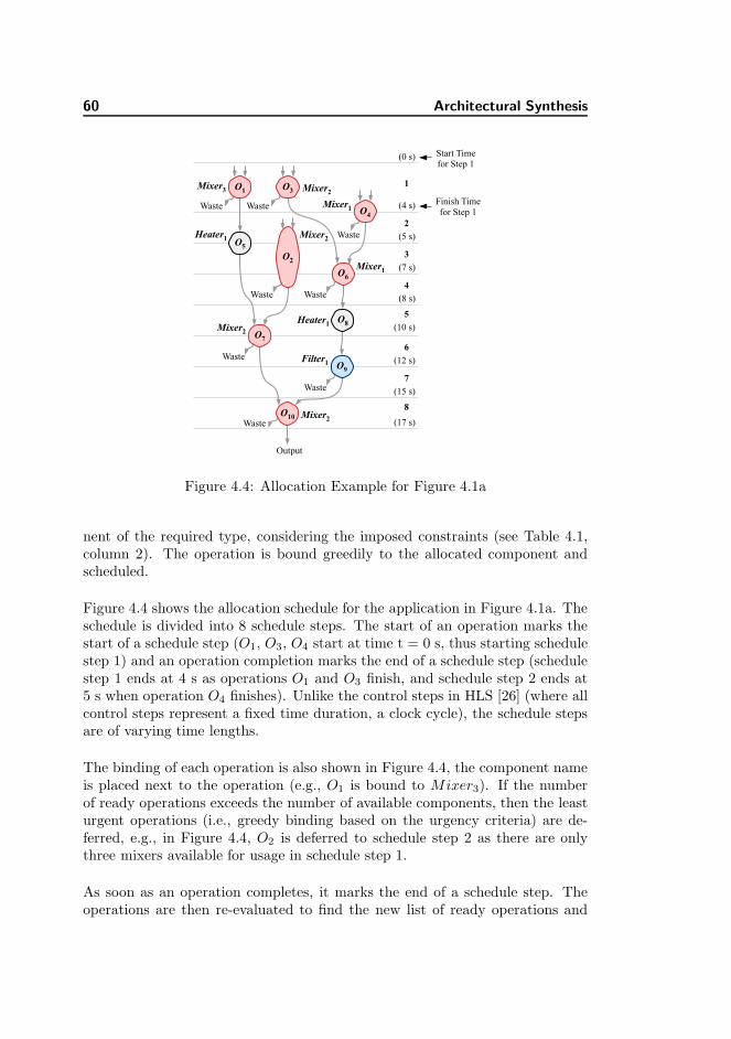
60 Architectural Synthesis

Figure 4.4: Allocation Example for Figure 4.1a

nent of the required type, considering the imposed constraints (see Table 4.1,column 2). The operation is bound greedily to the allocated component andscheduled.

Figure 4.4 shows the allocation schedule for the application in Figure 4.1a. Theschedule is divided into 8 schedule steps. The start of an operation marks thestart of a schedule step (O1, O3, O4 start at time t = 0 s, thus starting schedulestep 1) and an operation completion marks the end of a schedule step (schedulestep 1 ends at 4 s as operations O1 and O3 finish, and schedule step 2 ends at5 s when operation O4 finishes). Unlike the control steps in HLS [26] (where allcontrol steps represent a fixed time duration, a clock cycle), the schedule stepsare of varying time lengths.

The binding of each operation is also shown in Figure 4.4, the component nameis placed next to the operation (e.g., O1 is bound to Mixer3). If the numberof ready operations exceeds the number of available components, then the leasturgent operations (i.e., greedy binding based on the urgency criteria) are de-ferred, e.g., in Figure 4.4, O2 is deferred to schedule step 2 as there are onlythree mixers available for usage in schedule step 1.

As soon as an operation completes, it marks the end of a schedule step. Theoperations are then re-evaluated to find the new list of ready operations and

4.5 Synthesis Strategy 61

Figure 4.5: Schematic

the process is repeated. Table 4.1 shows the list of allocated components. Allimposed resource constraints have been fulfilled. All components have beenused in their maximum allowed number except the heater. Only one heaterhas been allocated considering the requirement, compared to the 2 heater unitsthat were allowed by the user. At this stage, the routing latencies are notyet known. The actual values of the routing latency are generated after theplacement and routing is complete. A set of input and output ports is allocatedfor each component in order to serve as the source and sink point during flowpath execution. Metering units are used to create discretized samples of unitvolume. The number of metering units allocated depends on the maximumpossible external inputs that can be executed in parallel. In the current case,a maximum of three external inputs are taken in parallel in schedule step 1(Figure 4.4) and thus three metering units have been allocated.

4.5.1.2 Schematic Design

In the next step, we extract the schematic design from the generated binding andscheduling information (analogous to data path generation in HLS [26]). Eachschedule step (Figure 4.4) is scanned to find the input source of the utilized com-ponents and a corresponding net is placed between the component and the inputsource. For example, Heater1 in schedule step 5 gets an input from Mixer1and gives an output to Filter1, therefore it is connected to both components.The extracted component interconnection scheme is shown in Figure 4.5.

Next we connect input and output ports to each component to serve as the sourceand sink point. Metering units are placed at the fluidic sample input ports.Storage units are needed to store intermediate results of operations [85]. Unlikein HLS (where registers are required at every control step [26]), biochips requirestorage only under special conditions. Consider an operation Ox bound to acomponentMy that finishes execution. If another operation gets bound toMy inthe next schedule step and the successor operation of Ox has not been scheduled

62 Architectural Synthesis

yet, then the output of Ox will need to be moved to the storage. Each storageunit is capable of storing multiple fluid unit samples, depending on the number ofstorage channels inside the unit. Since the routing latencies are not yet known, itis not possible to accurately assess which components would require the storageunit usage. For now, the storage unit is is connected to all components and thedesigner specifies the maximum capacity of the unit. Unnecessary connectionsand extra storage channels are removed after the application mapping step. Thefinal component interconnection configuration is shown in Figure 4.1b.

The flow path set F and the corresponding routing constraints K are also gen-erated in this step. The flow path set for the biochip architecture in Figure 4.1bis shown in Table 4.2. The source-sink path for each flow path and the routingconstraints are also shown.

4.5.2 Physical Synthesis

This stage takes the allocation U , the netlist, component library L and thedesired layout size as input and performs placement and routing (Zf , Rf , Zc,Rc), determining any additional constraints in the set K and the routing lengthsof the flow paths (that are used to calculate the routing latencies c). We use agrid-based approach to perform physical synthesis. The grid size is dictated bythe design rules and the component sizes on the grid are calculated accordinglyusing their dimensions given in the component library. The design rules imposedby the foundry and followed during the physical synthesis are summarized inTable 4.4. The placement and routing phases are divided into two stages:

4.5.2.1 Flow Layer

According to the problem formulation from Section 4.3, the placement and rout-ing should be done such that the application completion time is minimized.However, this would require using the mapping and scheduling (Section 4.5.3)as the cost function, which is too time-consuming. Instead, we use the to-tal channel length and the number of net intersections as the cost function.Minimizing the channel length minimizes the routing latencies, in turn mini-mizing the application completion time. Similarly, minimizing the number ofnet intersection minimizes the number of routing constraints, allowing more flowpaths to be executed in parallel. This will not lead to the optimal result, butwill reduce the application completion time. Furthermore, performing actualrouting to compare various placement solutions is impractical as routing is atime-consuming process. Therefore, we perform placement and routing in sepa-

4.5 Synthesis Strategy 63

rate steps and use an estimation method (Manhattan distance between two pinsis the estimated channel length needed to connect them) to estimate the totalchannel length in order to judge the quality of the placement solution.

The placement of components such that the total channel length is minimizedis an NP-complete problem, for which a number of good heuristic techniqueshave been developed [69]. Considering the problem at hand, we use SimulatedAnnealing (SA) (one of the most used methods for cell placement in VLSI [69])for performing component placement on the chip. Various algorithms have beenproposed for routing over the years. We use Hadlock’s Algorithm (HA) [69] andextend it for the flow layer routing. HA is suitable for the current problem sinceit also uses a grid model approach, finds the shortest path between two vertices(if such a path exists) and is faster than the other algorithms in this category[69]. We extend HA to also consider the possibility of net intersections, ensuringa 100% routability. The quality of the solution is judged by the number of netintersections and the total channel length. Since HA is sensitive to the order inwhich the nets are routed, we iterate on HA, providing it a re-ordered netlist forevery iteration in order to achieve a routing solution that minimizes the totalchannel length and net intersections.

The routing latency corresponding to each flow path is also generated in thisstep. Routing latencies are calculated by using the routing length of each flowpath extracted from the architecture and the flow rate used on the chip. Weconsider a flow rate of 10 mm/s for all experiments in this chapter. If the flowpath length is 10 mm and the flow rate is set at 10 mm/s, then a unit volume ofliquid (10 mm length on the channel) traverses this flow path in 2 s, i.e., fromthe time the tip of the 10 mm unit sample enters the flow path till the time thetail leaves from it. The latency values are required while performing applicationmapping. Latency values generated for each flow path are shown in Table 4.2.

Physical Synthesis Algorithm.

Figure4.6 shows our algorithm for the physical synthesis of the flow layer. Thealgorithm takes the allocated component set M , the generated netlist List andthe component library L as an input, and returns the placement and routinginformation of the flow layer. The objective is to place all the components onthe chip and minimize the total channel length in order to reduce the routinglatencies, while satisfying the design rules. Figure 4.2 shows the flow layerplacement and routing scheme that comes out of our algorithm.

Simulated Annealing [69] (lines 1−17 in Figure4.6) is used for generating theplacement scheme. SA is a metaheuristic, which, starting from a random initialplacement of components (line 3), iteratively obtains a better placement schemeby performing moves (line 6), i.e., design transformations, (swapping, rotating

64 Architectural Synthesis

FlowPlaceAndRoute(M , List, L)

1 // Phase I: Flow Layer Placement2 Initialize T3 Znow

f = InitialPlacement(M , L)4 repeat5 for i=1 to TL do6 Z ′

f = moves(Znowf )

7 δ = cost(Z ′f ) − cost(Znow

f )8 if δ < 0 then9 Znow

f = Z ′f

10 else11 if random(0,1) < e−δ/T then12 Znow

f = Z ′f

13 end if14 end if15 end for16 T = α × T17 until <stop criterion is met>18 // Placement returns the best solution Zf in terms of the cost function19 // Phase II: Flow Channel Routing20 Rnow

f = RouteFlowLayer(Zf , List)21 cnow = cost(Rnow

f )22 repeat23 List = Re-order(List)24 R′

f = RouteFlowLayer(Zf , List)25 c′ = cost(R′

f )26 if c′ < cnow then27 cnow = c′

28 Rnowf = R′

f

29 end if30 until <stop criterion is met>31 return < Zf , Rnow

f >

Figure 4.6: Physical Synthesis Algorithm for the Flow Layer

or randomly changing component location on the chip) to modify the currentsolution. SA also accepts deteriorations in cost (lines 11−13) to a limited extentin an effort to obtain global optimum, in terms of the cost function used. Theplacement generated by SA Zf is given as input to the Hadlock’s Algorithm[69] (lines 20−30) to iteratively generate the routing. A re-ordered netlist isgenerated (line 23) in every iteration in order to cater for HA’s sensitivity tothe order in which the nets are routed. The best solution for the placement Zf

and the routing Rnowf is then returned (line 31).

4.6 Experimental Evaluation 65

4.5.2.2 Control Layer

Control layer placement and routing can be done using the same algorithms asdescribed for the flow layer. We aim to target this step in our future research.Since the number of control valves on these chips can be extremely high (com-mercial chip having more than 25,000 valves [66]) and the number of punchholes that can be made on the chip for connecting the control pins is limitedby the design rules [15], each valve cannot be connected to a separate controlpin. In the next chapter, we propose an approach for sharing the control pinsbetween valves in order to minimize the number of control pins.

Next, we map the application onto the synthesized architecture using the ap-proach given in Chapter 3. We use the same binding as the one generated duringthe schematic design (Figure 4.4). As shown in Figure 4.3, the application re-quires only one storage reservoir. The output of operation O5 is moved to thestorage since the heater needs to be reused for operation O8 before the successoroperation of O5 (which is operation O7) is released. The application executionis completed in 32.2 s.

4.6 Experimental Evaluation

We evaluate our proposed approach by synthesizing biochip architectures forthree real life assays and a set of four synthetic benchmarks (all given in Ap-pendix B). We implement these applications onto the synthesized chips anddetermine the application completion time. The algorithm was implemented inC#, running on a Pavilion laptop (HP dv6-2155dx) with Core i3, Dual Proces-sors at 2.13 GHz and 4 GB of RAM.

Table 4.5 shows our experimental results for real-life case studies. Column 1presents the application and column 2 shows the list of allocated components,

Table 4.5: Real-Life Applications

Allocated Chip Net Total Total

Appl. Units Area Length Inters. Valves δG

PCR ( 3, 3, 3, 0, 0, 0) 250 × 250 198 4 67 19.7 s

IVD ( 5, 5, 3, 0, 0, 3) 250 × 250 393 10 101 20 s

CPA ( 5, 5, 5, 0, 0, 3) 250 × 250 1360 51 295 72.7 s

EA ( 5, 5, 3, 1, 1, 0) 150 × 150 1917 63 311 32.2 s

66 Architectural Synthesis

in the following format: (Input ports, Output ports, Mixers, Heaters, Filters,Detectors). Columns 3−6 present the desired chip area, total length of the flowchannels, total number of net intersections and the total number of valves onthe chip, respectively. Chip area represents the area given by the user as input.Chip area and total channel lengths are scaled, with a unit length being equalto 150 µm, i.e., a total length of 10 given in Table 4.5 corresponds to 1500 µm.The number of valves are calculated by considering 1 valve for each I/O port,4 valves for each intersection (switch), 9 valves for each mixer, 6 valves foreach metering unit and 2 valves each for all remaining components. The lastcolumn presents the completion time δG of the application, in seconds, on thesynthesized architecture.

The first real-life assay we use is the PCR (polymerase chain reaction) mixingstage. The architecture details and the corresponding application completiontime are shown in row 1 of Table 4.5. Row 2 shows the architecture generated forMultiplexed IVD (in-vitro diagnostics). The third row shows a larger real-lifeapplication, a colorimetric protein assay (CPA, 55 operations). It uses a chipequipped with 295 valves to complete its execution in 72.7 s. The architecturaldetails given in row 4 are for the example application (EA) given in Figure 4.1a.

In the second set of experiments we have evaluated our proposed method usinga set of four synthetic benchmarks. The benchmark applications are composedof 10, 30, 40 and 50 operations. Table 4.6 shows the details of the synthesizedarchitectures considered and the respective application completion times.

For each application in Table 4.6, two sets of architectures were synthesized. Thefirst row presents results for the architecture synthesized under designer-givenconstraints (maximum number of components of a certain type is constrained),whereas, the second row presents the results of an unconstrained architecture,

Table 4.6: Synthetic Benchmarks

Allocated Chip Net Total Total

|O| Units Area Length Inters. Valves δG

10 ( 2, 2, 1, 1, 1, 1) 150 × 150 1813 45 211 39.9 s( 5, 5, 2, 1, 1, 1) 150 × 150 1926 68 324 35.7 s

30 ( 6, 6, 3, 2, 2, 1) 250 × 250 3575 122 573 64.5 s( 15, 18, 6, 4, 3, 1) 350 × 350 5243 124 665 46.1 s

40 ( 8, 8, 4, 3, 1, 2) 350 × 350 4799 151 716 69.8 s( 18, 20, 7, 5, 2, 3) 350 × 350 7452 171 889 59.5 s

50 ( 10, 10, 5, 2, 2, 2) 350 × 350 6522 177 839 81.25 s( 21, 24, 10, 4, 3, 3) 400 × 400 9366 213 1109 60.1 s

4.7 Summary 67

i.e., no constraints were placed on the number of components to be used. Al-location step for the unconstrained architecture case can be considered similarto ASAP Scheduling [56]. For all applications, the unconstrained architectureproduces a completion time that is smaller than that of the constrained archi-tecture. All experiments presented in this section took between 3 to 30 minutesto complete, depending on the complexity of the application. All benchmarksand architecture details can be found here [14].

4.7 Summary

In this chapter we have presented a top-down architectural synthesis approachfor flow-based microfluidic biochips. The proposed approach synthesizes a biochiparchitecture for a given biochemical application, such that the application com-pletion time is minimized. The synthesis process involves component allocation,design schematic generation, and the physical synthesis (placement and rout-ing) of the chip. The approach has been evaluated by synthesizing biochiparchitectures for three real-life assays and a set of synthetic benchmarks. Theproposed approach is expected to facilitate programmability and automationin the microfluidics domain, reducing human effort and minimizing the designcycle time.

Once the biochip architecture has been synthesized and the application map-ping step has been completed, the output of the application mapping block canbe used to synthesize input for the biochip controller. This will enable auto-matic execution of the given biochemical application on the synthesized biochiparchitecture. The following chapter discusses this topic in detail.

68 Architectural Synthesis

Chapter 5

Control Synthesis

In this chapter we focus on the “Control Synthesis” block of our proposed designmethodology (see Figure 1.6). We start off by presenting the related workand describing our contributions. The tasks involved in control synthesis areexplained in Section 5.3 and our solution strategy is presented in Section 5.4.We experimentally evaluate our strategy in Section 5.5.

5.1 Related Work

There are two steps of control synthesis: (i) control logic generation and (ii)control pin count minimization. Control logic generation means determiningwhich valves need to be opened or closed, in what sequence and for how long,in order to execute the application on the chip [65]. Currently, this is donemanually by the designers [81]. Generating control logic manually is inefficientand error-prone (similar to exposing the gate-level details in microelectronics).Moreover, as the chips become more complex and the assays more concurrent,the manual process will not scale.

The second step is the control pin count minimization. As discussed in Sec-tion 1.3.1, a valve is connected to a pressure source through a control pin (e.g.,

70 Control Synthesis

Figure 5.1: Microfluidic Multiplexer [55]

in Figure 1.3a, valve va is connected to the pressure source through control pinz1). A valve is pressurized (closed valve) or de-pressurized (open valve) by thepressure source connected to the control pin. Having a separate control pin forevery valve directly translates to a large pin-count for the chip, resulting in (i)high consumption of the chip area, and (ii) requirement of large, expensive andcomplex macro-assembly around the chip (each valve requiring its own pressuresource). High pin-count is a bottleneck to the scalability of these chips andtherefore needs to be minimized.

Microfluidic multiplexers [55] have previously been used to minimize the controlpin count. Consider that there are N flow channels on the chip requiring Nvalves to close them. If every valve gets a separate pin and therefore a separatepressure source, N pressure sources will be required. However, if it is known thatonly one of the N flow channels needs to be open at a time (all others need tobe closed), then a microfluidic multiplexer can be used. Such a multiplexer willrequire only 2log2N control pins for controlling N such flow channels [21], e.g.,8 pins will be sufficient to control 16 such flow channels as shown in Figure 5.1.Valves are vreated only where a wide control channel (red) intersects with aflow channel (blue). Narrow intersections do not create valves. In Figure 5.1,control channels with status 1 have the associated valves closed and the oneswith status 0 have the associated valves open. For the case shown, the valvesare activated such that flow channel 14 is open and all others are closed.

In order to perform the multiplexer-based optimization, the user is asked tomanually specify which flows on the chip will be used and if they will be usedin parallel or not [21]. Once the flows have been specified, then the multiplexeris used for sharing the control pins between flow channels that satisfy the abovecriteria. Manual flow specification requires the user to have complete under-

5.2 Contribution 71

standing of the chip as well as the application requirements. The manual inputprovided by the user can also easily result in under or over-constrained specifi-cations, resulting in inefficient minimization. Moreover, the multiplexers-basedminimization is only applicable if the criteria of “only one out of N flow chan-nels needs to be open at a time” is fulfilled. The control pin count minimizationproblem has been reduced to the graph-coloring problem (which is NP-hard) [21]but no solution or experimental results have been presented.

5.2 Contribution

We propose a top-down control synthesis framework for implementing biochem-ical applications on flow-based biochips. Given a biochip architecture and themapping implementation of a biochemical application on the biochip architec-ture, control synthesis consists of the following two steps: (i) control logic gener-ation and, (ii) control pin count minimization. We utilize the output of controllogic generation step and perform the minimization by sharing the control pinsbetween multiple valves, provided that those valves operate in unison through-out the entire application execution. Pin count minimization using multiplexersand our proposed approach can be performed one after the other in order toreach a good solution. Here, we do not perform multiplexing but consider thatthis may already have been done in the given biochip architecture.

Considering the computational complexity of the problem, we propose a TabuSearch [48] based optimization in order to minimize the pin count. Our frame-work does not require manual flow specifications from the user, decoupling theapplication design from control synthesis. To the best of our knowledge, thisis the first time an approach for the control logic generation for the mVLSIbiochips is being presented.

5.3 Biochip Control Synthesis

The following subsections explain the tasks involved in the biochip control syn-thesis. Our proposed solution is discussed in Section 5.4.

We use the biochip architecture given in Figure 5.2 and the application givenin Figure 5.3b as an illustrative example. The biochip has 4 mixers, 2 heaters,2 filters and 2 detectors. Table 5.1 shows the list of flow paths, their routinglatencies and the routing constraints for the architecture in Figure 5.2. Each

72

ControlSynthesis

Table 5.1: Biochip Flow Path Set (F), Control Layer Model and Routing Constraints (K)Flow Paths Control Layer Model Routing

Flow Path Closed Valves Open Valves ConstraintsF0−x = (In1, Mixer1), 2 s F0−1 4, 7, 67 1, 2, 3, 5, 6, 8, 9, 10, 68 K3−x : F10−x

F1−x = (Mixer1, Filter1), 2 s F0−2 3, 5, 67 1, 2, 4, 6, 7, 68, 8, 9, 10 K8−x : F12−x

F2 = (Filter1, Heater2), 2 s ... K10−x : F3−x

... F6−1 30, 33, 71 27, 28, 29, 34, 35, 36, 31, 32, 72 K12−x : F8−x

F6−x = (In2, Mixer2), 2 s F6−2 29, 31, 71 27, 28, 30, 33, 32, 72, 34, 35, 36... ...F11 = (In3, Heater1), 2 s F11 64 42, 43, 44, 63F12−x = (Heater1, S1, Mixer3), 3 s ...

5.3 Biochip Control Synthesis 73

Figure 5.2: Biochip Architecture Example

flow path has an associated control layer model (given in Table 5.1) that containsthe details required for its utilization, i.e., the switch and the pump activationdetails. Figure 5.3a shows the schematic view for the area marked as Region Ain Figure 5.2. For the flow path F0−1 (1 for referring to the upper half of themixer) that goes from In1 to Mixer1 (as shown in Figure 5.3a), the valve set4, 7 needs to be closed and the valve set 1, 2, 3, 8, 9, 10, 5, 6 needs to beopened. The same is given as the control layer model of F0−1 in Table 5.1. Apumping action then moves the fluid from In1 to the Mixer1 upper half. Forthe biochip architecture in Figure 5.2, we consider that all the flow paths havetheir own dedicated off-chip pumps. The pumps can, however, be easily sharedbetween flow paths. In that case, the flow paths that share a pump will becomemutually exclusive and will be listed as such under the routing constraints.

The components in the architecture also have control layer models. For exam-ple, Mixer1 in Figure 5.3a is a pneumatic mixer (introduced in Section 2.1.1)implemented using nine microfluidic valves, numbered 2 to 10. The valve set8, 9, 10 acts as an on-chip pump. The valve set 2, 3, 4 and the valve set5, 6, 7 act as switches. The two switches facilitate the inputs and outputs,and the pump performs mixing.

The mixer has five operational phases. The first two phases represent the inputof two samples for mixing (filling the upper and lower half of the mixer), followedby the mixing phase (Mix). The mixed sample is then transported out of themixer in the last two phases, emptying the two halves.

In order to perform mixing (once both halves are filled), the mixer input andoutput valves 2, 6 are closed while valves 3, 4, 5, 7 (see Figure 5.3a) are

74 Control Synthesis

(a) Region A in Figure 5.2 (b) Application Graph

Figure 5.3: Schematic View and Application Example

opened and the mixing operation is initiated. Valve set 8, 9, 10 acts as aperistaltic pump. Closing valve 8 inserts some pressure on the fluid inside themixer, closing valve 9 creates further pressure, then as valve 10 is closed valve8 is opened again. This forces the liquid to rotate clockwise in the mixer. Thevalves are closed and opened in a sequence such that the liquid rotates at acertain speed accomplishing the mixing operation. The control layer of themixing phase is a part of the component model. Table 5.2 shows the controllayer model for all components in the biochip in Figure 5.2. The control layerdetails are only for the functional phase of the component. For example forMixer1, the control details are for the Mix operation for which the valve set2, 6 is closed, 3, 4, 5, 7 is opened and 8, 9, 10 is in the mixing state(opening and closing in a predefined sequence). Valve sequences for the heaters,filters and detectors are also given. In addition to these valve activations, therelevant component also needs to be activated, e.g., optical sensor present inthe detector needs to start operation as soon as the associated valves have beenactivated.

The input and output phases of the components are modeled using flow paths(and their associated control layers) in the architecture model. For example, theinput to Mixer1 from In1 in Figure 5.3a is modeled by the flow path F0−x (seeTable 5.1) and its activation is done using the associated control layer. Notethat the mix valves (e.g., valve set 8, 9, 10 for Mixer1) need to stay open forthe input and output phases of the mixer. Mix valves are active only when the

5.3 Biochip Control Synthesis 75

Table 5.2: Component Control Layer Model for Figure 5.2Component Open Closed Mixing

Valves Valves ValvesMixer1 3, 4, 5, 7 2, 6 8, 9, 10Mixer2 29, 30, 31, 33 28, 32 34, 35, 36Mixer3 49, 50, 51, 53 48, 52 54, 55, 56Mixer4 19, 20, 21, 23 18, 22 37, 38, 39Heater1 - 43, 44 -Heater2 - 13, 14 -Filter1 - 11, 12 -Filter2 - 57, 58 -Detector1 - 40, 41 -Detector2 - 24, 25 -

mixing is intended and need to be kept open after the mixing is done, until thedesired mixed fluid has been taken out emptying the mixer.

5.3.1 Control Logic Generation

Generating the control logic η means deciding which valves to close/ open, inwhat sequence, at what time and for how long, in order to implement a bio-chemical application G on the chip architecture A. A mapping ψ =< B,X >(binding and scheduling information) of the application on the biochip archi-tecture is given as input. Figure 5.4 shows the schedule X after mapping theapplication in Figure 5.3b on the biochip in Figure 5.2. The schedule is depictedas a Gantt chart, where we represent the operations and fluid routing phases asrectangles, with the lengths corresponding to their execution times. The starttime and the end time for the flow paths and operations in the schedule arecalled time steps, i.e., 0 s and 2 s in Figure 5.4 are considered time steps sincethey mark the start/ end time of the flow paths, whereas, 1 s is not a time step.

The control logic η is represented in a tabular form and contains the activationstatus of all valves on the chip, for all time steps of the schedule. The controllogic presented in Table 5.3 gives the activation status of the valves shown inFigure 5.3a for the schedule (given in Figure 5.4) duration 0 to 8 s.

Each row in the Table 5.3 represents the activation status of a valve. Firstcolumn contains the valve number and the remaining columns represent theactivation status of the valve for the time steps present in the schedule. Forexample, the first row in Table 5.3 represents the activation status of valve 1. A

76 Control Synthesis

Figure 5.4: Example Schedule

0 as activation status represents an open valve, 1 a closed valve and X representsa don’t-care, i.e., the valve may be opened or closed without having any influenceon the application execution. For example, valve 1 (row 1 in Table 5.3), isopened at time 0 s, stays open at 2 s and then its status changes to a don’t-careat 4 s. This is because from 0 to 4 s, F0−1 and F0−2 are executed, as shownin the schedule in Figure 5.4, filling the upper and lower halves of Mixer1 (seeTable 5.1). At 4 s, both fluid samples are inside the mixer, therefore valve 2closes in order to start the mixing operation (valve 2 status changes to 1 at4 s in Table 5.3). Once valve 2 is closed, the status of valve 1 switches to adon’t-care. This is because valve 1 and valve 2 are placed in series on the flowchannel (see Figure 5.3a) and once valve 2 is closed, opening or closing of valve1 has no impact on the application execution. The mix valves (e.g., valve 8, 9,10 in Mixer1) act as a pump in order to achieve mixing [55]. This pumping isalso included in η and for simplicity, it is shown as “Mix” in Table 5.3. The mixvalves are opened and closed at a certain frequency in order to achieve mixing,and this opening and closing continues even between time steps.

5.3.2 Pin Count Minimization

The biochip architecture may contain some valves that are never closed duringthe application execution. These valves are redundant and can be removed re-ducing the pin count, e.g., valve 1 in Table 5.3 is never closed and is thereforeredundant. Connecting each valve to a separate control pin results in too many

5.3 Biochip Control Synthesis 77

Table 5.3: Control Logic (η) Table - For Valves in Figure 5.3aValve Time Steps (s) ColorNo. 0 2 4 5 8 ...1 0 0 X X 0 ... -2 0 0 1 1 0 ... Color - 03 0 1 0 0 1 ... Color - 114 1 0 0 0 0 ... Color - 15 0 1 0 0 1 ... Color - 116 0 0 1 1 0 ... Color - 07 1 0 0 0 0 ... Color - 18 0 0 Mix Mix 0 ... Color - 149 0 0 Mix Mix 0 ... Color - 810 0 0 Mix Mix 0 ... Color - 2... ... ... ... ... ... ... ...27 0 0 X X X ... -28 0 0 1 1 1 ... Color - 329 0 1 0 0 0 ... Color - 630 1 0 0 0 0 ... Color - 131 0 1 0 0 0 ... Color - 632 0 0 1 1 1 ... Color - 333 1 0 0 0 0 ... Color - 134 0 0 Mix Mix Mix ... Color - 935 0 0 Mix Mix Mix ... Color - 436 0 0 Mix Mix Mix ... Color - 7... ... ... ... ... ... ... ...42 0 X X X X ... -43 0 1 1 X X ... Color - 1344 0 1 1 X X ... Color - 13... ... ... ... ... ... ... ...89 X X X X X ... Color - 4

pin-outs from the chip limiting the chip scalability. In order to minimize the pincount, a strategy is needed in order to share the control pins between differentvalves that perform in unison with each other throughout the application exe-cution schedule. For example in Table 5.3, valve 2 and valve 6 have identicalactivation sequence in all time steps and therefore, can share the same controlpin. Similarly, valve 1 and 2 also have the same sequence (X for valve 1 at timesteps 4 and 5 means that valve 1 can be switched to 1 or 0 without affecting theapplication execution) and can share the control pins.

78 Control Synthesis

5.3.3 Problem Formulation

Given (1) a biochip architecture modeled as a topology graph A, and (2) amapping ψ = < B,X > (binding and scheduling information) of an applicationG on the biochip architecture A, we are interested in performing the controlsynthesis for the given chip. Control synthesis consists of the following steps:(1) generating the control logic η needed to execute the application on the chip,and (2) minimizing the control pin count of the chip.

5.4 Synthesis Strategy

Figure 5.5 shows our algorithm which is explained in the following subsections.

5.4.1 Control Logic Generation

Control logic η is generated by fetching the control layer model of the biochipflow paths F and components M (part of the biochip architecture model A),and utilizing them to translate the mapping ψ into the valve activation sequence(line 2 in Figure 5.5). At every time step of the schedule X , we look at theactive flow paths and operations, fetch the associated control layer models andpopulate the table representing the control logic. The valves that need to beopened are given a status 0, the ones that need to be closed 1 and to the setof valves that are mixing the status “Mix” is allotted. All other valves are setas X (don’t-care) for this time step and then the algorithm moves on to thenext time step. For example at time step 2, operation O3 and flow paths F0−2,F6−2 are active, as shown in the schedule in Figure 5.4. Operation O3 is boundto Heater1, so we fetch the control layer model for Heater1 from Table 5.2according to which valves 43, 44 should be closed. The status for these valvesis therefore set to 1 at time step 2 in the control logic (Table 5.3). Similarlythe control layer models for the flow paths F0−2 and F6−2 are fetched fromTable 5.1 and the valves involved are set to either 1 or 0, depending on whetherthey needed to be closed or opened. All other valves (except the mix valves)are set to the status X for time step 2.

The mix valves are assigned a don’t care status X only when either both halvesof the mixer are empty, or when the mixed fluid in only one half of the mixerwas required for the application and that half has been emptied. When mixvalves (e.g., 8, 9, 10 for Mixer1) are set to X, the input and output valves ofthe respective mixer (2, 6 for Mixer1) need to be closed. This ensures that

5.4 Synthesis Strategy 79

ControlSynthesis(A, ψ, k, maxIter)

1 // Generate control logic2 η = GenCtrlLogic(F , M , ψ)3 // Algorithm for pin count minimization4 Gc = GenGraph(η)5 k = |Gc|, kIterate = 16 while f(s) > 0 and kIterate = 1 do7 // Generate initial solution8 s = Random(Gc)9 Initialize TL to φ, nrIter = 0, s∗ = s

10 while f(s) > 0 and nrIter < maxIter do11 BestMove(s′) = GenNbrSelectMove(s, TL)12 Update TL13 if f(s∗) > f(s′) then14 s∗ = s′, nrIter = 015 else16 nrIter++17 end if18 PerformMove s = s′19 end while20 (k, kIterate) = BSearch(f(s), k)21 end while22 return < η, GC , s∗, k>

Figure 5.5: Synthesis Algorithm

if these mix valves (e.g., 8, 9, 10 of Mixer1) share control pins with othermix valves (e.g., 34, 35, 36 for Mixer2) and a pumping action is performedbecause of this, the pumping affect is contained inside the mixer and does notaffect the rest of the chip operation.

5.4.2 Pin Count Minimization

The pin count minimization problem has previously been reduced to a graphcoloring problem (GCP) [21]. In GCP, the nodes in the graph need to becolored using minimum number of colors, in such a way that no two adjacentnodes have the same color. Finding the exact chromatic number (the minimumnumber of colors that can be used to color the graph nodes) is an NP-hardproblem [21]. Finding out if the graph can be covered with k colors is an NP-complete problem [48]. The problem has previously been reduced to a GCP,however, no solution or experimental results have been proposed.

80 Control Synthesis

5.4.2.1 Graph Generation

Before we generate the graph, we remove redundant valves, if any, from thebiochip architecture. Redundant valves are the ones that are never closed dur-ing the entire application execution, e.g., valve 1, 27 and 42 in Table 5.3 areredundant valves as their status is never set to 1. These valves can be removedfrom the biochip as their presence has no effect on the application execution.

Next, we create the graph GC(VC , EC) (line 4 of Figure 5.5) by considering eachvalve in Table 5.3 as a separate node V c in the graph (redundant valves arenot considered). An edge Ec is made between two nodes if a time step existsin the schedule for which the valves (represented by the nodes) have a differentactivation status. For example, the nodes representing valve 2 and valve 6will not have an edge between them as they operate in unison throughout theschedule as shown in Table 5.3, but an edge will be made between valve 2 and3 since their activation status vary at time step 2 (valve 2 is open and valve 3is closed). The graph is complete once all edges have been drawn. The graphfor Table 5.3 has 83 nodes (total valves were initially 89, 6 were found to beredundant and were removed) and 1312 edges.

5.4.2.2 Pin Count Minimization Algorithm

The problem for pin count minimization is now represented in the form of aclassical graph coloring problem (GCP). Once the colors have been assigned,the nodes that have the same color will share the same control pin.

GCP has been studied extensively and different approaches have been proposedto find a good quality solution. The simplest approach is the Greedy method [48]which takes the ordering of the nodes as input and colors them with the smallestcolor number, while satisfying the constraint that no two adjacent nodes shouldhave the same color. Greedy often performs poorly in practice since a good nodeordering is difficult to decide. DSATUR is another commonly utilized approachthat uses a heuristic to dynamically change the ordering of the nodes and thenuses the Greedy method for coloring [48]. Branch and bound algorithms [48]and semi-definite programming solutions for approximate graph coloring [41]have also been proposed. Considering the complexity of the problem, differentmetaheuristic techniques have also been used extensively for finding good graphcoloring solutions, especially when there is a large number of nodes [48]. Weuse a Tabu Search-based optimization scheme in order to perform the pin countminimization.

5.4 Synthesis Strategy 81

Tabu Search (TS) is a metaheuristic, based on the neighbourhood search, whichuses design transformations (moves) applied to the current solution in orderto generate a set of neighbouring solutions that can be further explored by thealgorithm [34, 37]. Our algorithm targets a k-GCP, i.e., finding a graph coloringusing k number of colors and then iterates to find the smallest value of k.

Given the graph GC(VC , EC) to be colored, the target of the algorithm is topartition the nodes into a fixed k number of subsets, such that no two adjacentnodes belong to the same subset. We start with a random solution s for thek-coloring (line 8 in Figure 5.5), which (typically) contains a high number ofedges in a conflict, i.e., the nodes connected by these edges have the same color.Using this as an initial solution the algorithm iterates to explore the solutionspace S, which is the set of all possible k-colorings of the graph.

In order to efficiently perform the search, TS uses memory to record moves thatare not allowed at the present iteration (called tabu list (TL)). The aim is toexclude moves that would cycle the search back to the local optima that hasalready been evaluated. A move remains tabu for a certain number of iterations(called the size of tabu list). Our algorithm starts with an empty TL and thebest known solution s∗ is initialized with the initial solution s (line 9).

Next, the algorithm generates neighbourhoods for the current solution s andpicks the best one from these based on a certain objective function (line 11). Aneighbour s′ is generated by selecting a random node x that is adjacent to anedge in conflict. Assuming x ∈ VCi, we choose a random color j 6= i and replacei with j to obtain s′. The objective function f(s) is given as:

f(s) =k∑

i=1

|ECi| (5.1)

(it measures the number of edges in conflict), where s ∈ S is the solution underevaluation, and ECi is the set of edges in conflict, having color i. The objectiveof the algorithm is to determine a k-coloring such that f(s) = 0. The best moveis the one that is not tabu and has the lowest f(s) value.

Our algorithm generates the tabu list as follows: whenever a node x is movedfrom VCi to VCj , the pair (x, i) becomes tabu, i.e., node x cannot be returnedto VCi for a certain number of iterations. However, in order to not prohibitattractive moves, our algorithm uses the aspiration criteria of allowing the tabumoves if they result in a solution s′ that is better than the currently known bestsolution s∗. The best move is selected and the tabu list is updated (line 11, 12).

The algorithm continues searching until it finds a solution for which f(s) = 0or until it reaches the maximum number of iterations without an improvement

82 Control Synthesis

Figure 5.6: Colored Graph

in the solution (number of iterations nrIter is reset and incremented in line 14and 16 respectively). Our algorithm uses binary search (half-interval search) toselect new value of k, as it iterates to find the minimum value of k for whichf(s) = 0 (line 20). When the minimum k is found, the algorithm stops andthe control logic η and the pin sharing information (Gc, s∗, k) is returned (line22). The graph generated for Table 5.3 has 83 nodes, i.e., 83 valves requiring83 control pins and therefore 83 off-chip pressure sources. After performingthe pin count minimization, only 15 control pins were found to be needed tocontrol these 83 valves and to execute the control logic given in Table 5.3. Lastcolumn in Table 5.3 shows the colors assigned to the valves (valves with thesame color share the control pin). A small section of the colored graph is shownin Figure 5.6 representing the pin sharing, e.g., valve 2 and valve 6 do not havean edge between them, hence they share the same color (and therefore the samecontrol pin). Complete graph is shown in Figure 5.7.

5.5 Experimental Evaluation

We evaluate our proposed approach by synthesizing real-life assays as well assynthetic benchmarks. The algorithm was implemented in C++, running onLenovo T400s ThinkPad with Core 2 Duo 2.53 GHz Processors and 4 GB RAM.

Table 5.4 shows the results. Column 1 shows the application name (for a real-life assay) or the number of operations in the application (in case of a syntheticbenchmark). The second column gives details of the biochip architecture in thefollowing format: (Mixers, Heaters, Filters, Detectors). The third column showsthe number of control pins originally needed and column 4 shows the numberof control pins needed once the redundant valves have been removed (the termNR in the table means Non-Redundant). Column 5 gives the final pin countafter the minimization has been performed.

The first real-life assay is PCR (polymerase chain reaction) mixing stage thathas 9 mix operations and is used in DNA amplification [14]. Next, real-life ass-

5.5

Experim

entalEvaluatio

n83

Figure 5.7: Complete Graph for Table 5.3

84 Control Synthesis

Table 5.4: Experimental ResultsAppl./ Allocated Total NR OptimizedNodes Units Pins Pins PinsPCR (4, 0, 0, 0) 73 52 12IVD (6, 0, 0, 6) 65 65 1210 (4, 2, 2, 2) 87 83 1520 (12, 4, 3, 1) 164 145 3830 (17, 6, 4, 3) 212 201 4740 (21, 9, 6, 4) 269 197 7450 (26, 12, 7, 5) 329 240 61

ay Multiplexed IVD (in-vitro diagnostics) has a total of 12 operations and isused to test fluid samples from the human body. The synthetic benchmarkapplications are composed of 10 up to 50 operations. In all cases, the pin countis reduced by more than 70%, e.g., for the 10 node application it goes down from87 to 15, an 82% reduction in pin count. The parameter values were determinedby tuning. Size of TL was set to 7 and the number of neighbours/ sample to 15.The algorithm execution time depends on the chosen value of k and the size ofthe problem. On average, for each value of k, the algorithm iterates for 2 to 4minutes. All architectures and benchmarks can be found here [14].

5.6 Summary

In this chapter, a top-down control synthesis framework for implementing thebiochemical applications on the flow-based biochips has been proposed. Ouralgorithm generates the control logic needed to execute the application and usesa Tabu Search-based optimization in order to minimize the control pin count.The minimization is targeted at efficiently utilizing the chip area and reducingthe macro-assembly around the chip. The framework has been evaluated usingreal-life applications as well as a set of synthetic benchmarks. The proposedapproach is expected to facilitate programmability and automation, and enhancescalability of the flow-based biochips.

Chapter 6

Experimental Throughput

Maximization for

Cell Culture Biochips

The term “cell culturing” refers to the process of growing cells outside theirnatural environment (in vitro). This allows the study of complex cellular mech-anisms without requiring the usage of laboratory animals. Cell culturing pro-vides biological insights into cells and tissues bringing exciting opportunities forstem cell research, drug discovery (e.g., for cancer) and a wide range of otherapplications in the biomedical and pharmaceutical industry.

In cell culturing, an experiment is defined as the exposure of a cell colony toa sequence of fluidic compounds and monitoring its response. For example,cancer cells can be exposed to a sequence of fluidic compounds (possible drugs)in order to monitor which compounds (or which sequence of compounds) hasthe most desired effect. Exposing cells to all possible sequences of the fluidiccompounds is called a full factorial experiment and exposing them to a fractionof all sequences is called a fractionally factorial experiment [63].

Drug discovery is one of the foremost applications of cell culturing. The firststep to drug discovery is to screen millions of compounds for effects on one tar-get (e.g., a cell colony). Since there are millions of compounds to screen for,

86

Experimental Throughput Maximization for

Cell Culture Biochips

only a fractional factorial design is utilized. Once the lead compounds havebeen identified, a full factorial design is initiated. Full factorial experimentsare expensive in terms of time and cost and hence need to be performed usinghigh throughput techniques to conserve resources [75]. Having high through-put means performing as many experiments as possible using the available cellcolonies and fluidic compounds, within the limited amount of time.

Biologists have traditionally used cell culture platforms equipped with microwellplates, where the cells are cultured inside the wells. Seeding, growing, feedingand analysing the cell cultures inside the wells manually, requires many hoursof repetitive and painstaking work. Therefore, cell culture platforms have beenautomated using robotics. Robotics-based automated cell culture systems arebeing used today to increase the throughput by using their ability to managea large number of experiments, e.g., a cell culture system featuring a CRS 465robotic arm can handle up to 504 microwell plates [42]. Flow-based biochips offera promising alternative to robotic microwell cell culture systems [27]. Biochipscan mimic both the complex biochemistries and the geometry of environmentsfound in organisms. At the same time, transport of fluids and soluble compoundsis regulated through the microfluidic channels creating new opportunities for thespatial and temporal control of cell growth and stimuli [28].

Our focus in this chapter is on modeling a cell culture biochip architecture andoptimizing how a biochemical application is executed on these biochips, suchthat the experimental throughput is maximized. The architecture modeling ispresented in Section 6.1.1 and the optimization problem in Section 6.1.2.

Several microfluidic cell culture platforms have been proposed. A large numberof cell culture platforms contain biochips that have been fabricated using PMMA(polymethyl methacrylate) as the substrate. PMMA is more suitable thanPDMS in culturing certain cell types. We start by considering PMMA-basedcell culture biochips and later explain the mVLSI-based ones. The techniquesproposed in this chapter are applicable to both PMMA and mVLSI biochips.

Consider the platform shown in Figure 6.1 [76]. It has a PMMA biochip onwhich the cells are cultured, inlet reservoirs containing compounds to which thecells are exposed, pumps that are used to push the compounds into the chip andoutlet reservoirs that collect the compounds when they come out after passingover the cells. The system is programmable, providing simultaneous softwarecontrol of the pumps and the microscope for automated image analysis.

The cell culture biochip architecture, shown in Figure 6.1b, provides the op-portunity for performing these high throughput experiments. The architectureshown in the figure can hold 64 cell colonies and therefore 64 experiments simul-taneously (8×8 matrix, see Section 6.1.1 for details). All the experiments being

87

(a) Biochip Platform [86]

(b) Laminar Flow Biochip

Figure 6.1: Biochip Platform and Architecture

carried out (64 in this case) in the chip are collectively considered as one experi-mental stage. An experiment is considered unique if it is not repeated anywhereon the chip. The biochip throughput depends on the number of unique experi-ments carried out on the chip. Note that several experimental stages might benecessary to achieve a certain target objective. A new chip (or the same chipmight be washed and reused) has to be used for the next experimental stage.

An experimental stage has two steps. (1) In the first step the cell colonies areinserted and placed on the chip. The placement is fixed for an entire experi-

88

Experimental Throughput Maximization for

Cell Culture Biochips

mental stage. For example, in Figure 6.1b, different cell colonies (Q) are placedon the chip. (2) In the second step, the soluble compounds are inserted usingeither the top-to-bottom route (insertion from the top inlets: In1 to In8 inFigure 6.1b, exit using the bottom outlets) or the left-to-right route. When acompound is inserted from an inlet (e.g., In2), it traverses through all coloniesin its way till it reaches the outlet (e.g., the colony set (Q−, Q9, Q7, Q1, Q6,Q1, Q6, Q

+) in the second column in Figure 6.1b), influencing all 8 experiments(every cell colony is a separate experiment). The soluble compounds are manu-ally placed in inlet reservoirs (see reservoirs in Figure 6.1a). However, they aretransported to the biochip automatically using pumps according to the insertionschedule determined offline, i.e., the schedule is decided before the experimentis performed. The pump can fetch from any desired inlet reservoir. The pumpsare controlled using a programmable custom-made electrical controller. The cellplacement pattern (1) and the compound insertion schedule (2) determine thenumber of unique experiments in an experimental stage. The serialized insertionof compounds (i.e., a compound inserted from an inlet affects all colonies placedbetween that inlet and the designated outlet) reduces the probability of havinga high number of unique experiments.

Today the experimental design, i.e., deciding the placement pattern of the cellcolonies on the biochip and the schedule of the stimuli insertion (which com-pounds to insert, in what sequence, and from which inlets), is done manuallyresulting in undesired repetitions of experiments on the chip, reducing the overallthroughput. We propose an optimization approach to automate the cell culturebiochip experimental design such that the experimental throughput is maxi-mized. Maximizing the throughput increases system productivity, saving time(one cell culture experiment can take days to complete) and reducing costs; thepurified proteins and compounds used in the experiments are highly expensive.

6.1 System Model

6.1.1 Biochip Architecture

Figure 6.1b gives a high-level representation of a biochip architecture [76] for cellculturing. The biochip itself is one big chamber (imagine a very wide microfluidicchannel) with 8 inlets at the left and 8 at the top, and 8 outlets at the rightand 8 at the bottom. The biochip uses the laminar flow property [86] which isdefined as the flow of fluids in parallel layers without any disruption between thelayers. This means that when different compounds are pushed in from differentinlets (e.g., from In1 to In8), because of the microscale volumes they flow in

6.1 System Model 89

parallel without mixing thus creating 8 parallel flows. Similar effect is obtainedwhen inlets on the left (In9 to In16) are used. Only one set of inlets can beused at a time. The biochip is represented as an AR×AC matrix (AR rows andAC columns, e.g., for the chip in Figure 6.1b, AR = AC = 8). Each element ofthe AR ×AC matrix hosts a cell colony. The off-chip valves V1 and V2 controlthe flow to the outlets.

Before starting an experiment, the locations on the chamber where the cellcolonies are to be placed are tagged using DNA spotting technique. Then, tocarry out the experiment, first, valve V2 is opened and valve V1 is closed, allow-ing different cell types to be pumped into the large chamber. Due to laminarflows, eight corresponding stripes of cells are produced. After sedimentation,cells adhere to the bottom of the chip according to the DNA spotting. Then,valve V2 is closed and valve V1 is opened, allowing eight soluble compoundsto perfuse over the cells in the perpendicular direction creating simultaneousexperiments in the chip. It is also possible to insert soluble compounds usingthe same inlets from which the cells were initially inserted (valve V1 closed, V2open), but only one type of inlets can be open at a time.

Two special types of cell colonies, positive (Q+) and negative (Q−) controls(selected based on the application being executed on the chip, i.e., dependingon the cell colonies and the input compounds), are used to ensure the quality ofcompounds being inserted into the chamber and to guarantee that the conditionsin the chamber are uniform [77]. The actual size of the chip here is 8×8, butsince the controls need to be placed at the boundary locations, therefore theactive area (on which the cell colonies under test are placed) is reduced to 6×6.

As mentioned, the biochip shown in Figure 6.1b has one large chamber and relieson the laminar flow properties of the liquids for ensuring that the inserted cellsand compounds do not mix with each other. This is prone to different faults,e.g., if an air bubble enters the chip from one of the inlets, it will not just affectthe cell colonies in front of the inlet it entered from but instead all cell colonieson the chip can become enclosed in the air bubble. This will result in the failureof of all experiments on the chip.

Another option would be to isolate the rows and columns in the chip, i.e., haveindependent chambers instead of one large chamber. The mVLSI technologyprovides such an option offering more control, as is the case with the biochipshown in Figure 6.2. The biochip shown in the figure is shaped in the form ofa 20×20 matrix and is used to perform 400 distinct PCR reactions (i.e., it isnot used for cell culturing) [51]. Each vertex in the matrix contains a reactor,so there are 400 reactors (20×20) in total. Each row of reactors is connected toa separate input port through which primers may be loaded. Each column cansimilarly load the reactors with different DNA templates [51].

90

Experimental Throughput Maximization for

Cell Culture Biochips

Figure 6.2: PCR Biochip with AR = AC = 20 (Scale Bar 6.4 mm) [51]

Figure 6.3: Cell Culture Chip: Schematic View

6.1 System Model 91

Table 6.1: Flow Path Set (F) and the Routing Constraints (K)Flow Path Set Routing ConstraintsF1 = (In1, S1, Ch1, S9, Ch2, S17, Ch3, S25, Ch4, ) K1: (K9 to K16)S33, Ch5, S41, Ch6, S49, Ch7, S57, Ch8, S65, Out1) ...F2 = (In2, ..., Out2) K8: (K9 to K16)... K9: (K1 to K8)F15 = (In15, ..., Out15) ...F16 = (In16, ..., Out16) K16: (K1 to K8)

The chip has 2,680 valves in total, placed horizontally and vertically. Since theflows are activated either vertically (top to bottom) or horizontally (right toleft) therefore all these valves are controlled by only two control pins connectedto two independent pressure sources, i.e., all valves required to be closed forvertical flows are controlled by one pressure source since they are always closedat the same time. Same applies to the valve activation for horizontal flows [51].

Figure 6.3 shows the schematic view of the mVLSI architecture that we considerfor a cell culture biochip, based on the architecture discussed above (Figure 6.2).The architecture shown has 64 chambers (8×8) for placing 64 cell colonies (samenumber of cell colonies as for the chip in Figure 6.1b). This architecture offersisolated chambers and more control. The chip uses a network of 144 switchesto control 64 cell culture chambers. The flow paths and the associated routingconstraints are shown in Table 6.1. Switch set S73 to S144 is closed for ex-ecuting flow paths F1 to F8 and switch set S1 to S72 is closed for executingflow paths F9 to F16. Therefore all 144 switches can be controlled using only 2control pins, i.e., only 2 external pressure sources are needed. We consider thatthe chip shown in Figure 6.3 is used in the platform in Figure 6.1b.

6.1.2 Experimental Design

As stated earlier, exposure of a cell colony to a sequence of soluble compoundsand monitoring its reaction is termed as an experiment. All the experimentsbeing carried out in a chip are collectively considered as one experimental stage.In order to explain the experimental design process, we consider a 6×6 cellculture biochip that has an active area of 4×4. The chip is used to carry outexperiments in n = 3 experimental stages, Figure 6.4 (a) to (c).We consider aset Q of two cell colonies (Q1 and Q2) and a set J of three compounds to beinserted (J1 to J3). We would like to expose the cells to the compounds, in anyorder. The exposure time per compound is fixed. However, since we allow thecompound to be repeated in an exposure sequence, we can thus increase the

92

Experimental Throughput Maximization for

Cell Culture Biochips

exposure time for the same compound. The maximum number of experimentalstages to be used is generally decided based on the available budget (experimentsare highly expensive).

The placement of cell colonies on the biochip is given by the matrix Z; seefor example Z1 in Figure 6.4a. The sequence of compounds is captured by theschedule Y, composed of < YR, YC , YZ >. The compounds can be insertedeither from left to right (row-wise) or from top to bottom (column-wise). Twomatrices YR and YC represent the compound placement at the insertion point,row-wise and column-wise, respectively. The set YZ represents the sequence inwhich the compounds are inserted. A “1” in YZ marks a column-wise insertionwhereas a “0” represents a row-wise insertion, see for example Y1 = < Y 1

R, Y1C ,

Y 1Z > in Figure 6.4a.

Through experiments, we have to find out the sequence of compounds thatprovide the desired result for a specific cell colony. To maximize the number ofcombinations applied to a cell colony, it is important to perform as many uniqueexperiments on the chip as possible. A unique experiment is one which is notrepeated (in another part of the chip, or during another experimental stage).

Consider the cell colony Q2 placed in the top left corner in Figure 6.4a. Thenumber of compounds to which the colonies are to be exposed is consideredto be fixed to 3 by the biologist. Y 1

Z in Figure 6.4a is 1, 0, 1. This meansthat the first compound insertion will be made from YC , the second from YRand the third again from YC . Therefore, Q2 placed at the top left corner willbe exposed to the following compounds: J1 (from YC), J3 (from YR), J2 (fromYC), denoted as “132”. There are 16 colonies placement location on the chip,8 are filled with Q1 and 8 with Q2. Based on the schedule Y1 = < Y 1

R, Y1C ,

Y 1Z > given in Figure 6.4a, following experiments are performed (sequence of

the experiments listed below is a row by row listing from the matrix):

Q1 : 233, 331, 122, 122, 112, 112, 233, 331

Q2 : 132, 132, 223, 321, 213, 311, 132, 132 (6.1)

where we have underlined the experiments that have been repeated. Repeti-tion of experiments results in inefficient utilization of the chip. This results indiminished system productivity and increased expenses, both in terms of timeand cost. Therefore, efficient experimental design is essential. Note that al-though our model uses two matrices, YR and YC to capture the compounds,only one such matrix is used in the implementation. The set YZ will determineif a particular row in this matrix is fed row-wise or column-wise.

Considering an AR ×AC biochip, the maximum number of unique experimentsthat can be carried out in one experimental stage is given by the active chip

6.1

Syste

mModel

93Figure 6.4: Motivational Example

94

Experimental Throughput Maximization for

Cell Culture Biochips

area: A′R × A′

C , where A′R = (AR − 2) and A′

C = (AC − 2). Therefore, forFigure 6.4a, the maximum utilization Umax of the biochip is: Umax = 4×4 =16. The maximum number of combinations possible for a given colony dependson the experimental specifications, captured by the set of compounds J andthe number of compounds I in an exposure sequence and is equal to (|J |I),where |J | is the number of elements in the set J . For the experiments inFigure 6.4a, (|J |I) = 27, the total number of combinations of I = 3 itemstaken from a set of three elements J = J1, J2, J3. The number of possiblecompound combinations (|J |I) for a certain cell colony is typically larger thanthe maximum chip capacity Umax, which has to be divided among several cellcolonies. For the placement in Figure 6.4a, colony Q1 can use only half of thetotal capacity, Umax / 2 = 8. Therefore, to achieve a wider coverage from the setof 27 unique experiments per colony, it is imperative to have more experimentalstages even if the chip is fully utilized for the first stage, i.e., all 16 experiments(8 per colony) carried out in the first stage are unique. In the current case, thebiologist has specified 3 experimental stages. This means that in the ideal case,24 out of the 27 unique experiments can be achieved for each colony. The samebiochip may be washed and manually reloaded with cell colonies for reuse inmultiple experimental stages.

6.2 Problem Formulation

The problem we are addressing in this chapter can be formulated as follows.Given (1) a cell culture biochip architecture model consisting of an AR × AC

matrix representing the cell culture chip chambers, (2) a set of compounds Jthat are to be inserted from the inlets, (3) a set of cell colonies Q that are to beplaced on the cell culture chambers, (4) the number of compounds per exposuresequence I, and (5) the total number of experimental stages n to be performed,we are interested in designing each experimental stage Ωi, i = 1...n, such thatthe experimental throughput γ is maximized.

Designing an experimental stage Ωi < Zi, Yi > means deciding for each stagei on: (1) the placement Zi of the cell colonies from the set Q and (2) thecompound exposure schedule Yi = < Y i

R, YiC , Y

iZ >. The throughput of a cell

culture biochip is defined as:

γ =|EU |

min(n× Umax, (|J |)I × |Q|)(6.2)

where |EU | is the number of elements in the set EU of unique experiments over nstages, considering the synthesized design Ω. The maximum number of uniqueexperiments is bounded by (i) the chip capacity, n × Umax, and by (ii) the total

6.2 Problem Formulation 95

number of possible combinations, considering all cell colonies Q, (|J |I) × |Q|,whichever of the two values is smaller. Therefore, γ represents a percentage ofunique experiments obtained through our design Ω to the maximum possible,given the chip capacity or the number of combinations. Note that a 100%throughput might not be possible to obtain, and we have no way of knowingmaximum possible throughput unless we obtain the optimal design.

Let us use the example in Figure 6.4 to illustrate our problem. In Figure 6.4,we have A′

R = A′C = 6 − 2 = 4, Q = Q1, Q2, J = J1, J2, J3, I = 3 and n = 3.

Let us suppose we start from the configuration shown in Figure 6.4a, where weassume that the placement Z1 and schedule Y1 have been decided as depictedin the figure. All the experiments obtained in this first stage Ω1 = < Z1, Y1 >have been listed in eq. 6.1. As shown, for Q2 5 out of the total 8 experimentscarried out are unique and for Q1 only 4 experiments are unique. The remainingexperiments (underlined) are repetitions. Therefore, the chip capacity for thisstage is poorly utilized.

In order to increase to number of unique experiments we have to carefully designthe second stage Ω2 = < Z2, Y2 >. For the second stage, the same biochip canbe used but, as stated earlier, it needs to be washed and reloaded with cellcolonies at the decided placements. A simple way to generate a stage Ωi isto modify a previous stage Ωi−1 using a certain set of rules. We have decidedto roll over the placement Zi−1 and the contents of the schedule Yi−1 in thehope to increase the number of unique combinations. Thus, we obtain the stagedesign Ω2 given in Figure 6.4b, where Z1, Y

1R, Y

1C and Y 1

Z from Figure 6.4a areall rolled to the right, i.e., all the contents are shifted right and the ones in theright most position are moved to the first entries on the left. The experiment isrun again and the following experiments are generated:

Q1 : 232, 312, 121, 121, 123, 123, 232, 312

Q2 : 122, 122, 231,311, 233, 313, 122, 122 (6.3)

The experiments underlined are repeated in the same stage and the ones markedin bold have already been covered in the previously conducted experimentalstage listed in eq. 6.1. Each cell colony, Q1 and Q2, now has 4 more uniqueexperiments, whereas ideally, 8 unique experiments could have been achieved inthis experimental stage. Again, the chip capacity has been utilized poorly forthis stage as well and needs to be improved.

More variations are now required in the experimental settings in order to in-crease the probability of covering more unique experiments. Thus, for the thirdexperimental stage, a top-to-bottom roll is performed on the settings in Fig-ure 6.4b, i.e., all the contents are shifted one step towards the bottom and theones at the bottom position are moved to the first entries on the top. Since the

96

Experimental Throughput Maximization for

Cell Culture Biochips

top-to-bottom roll cannot be performed on the Y 2Z (1-D array), it is rolled to

the right instead. The new settings are shown in Figure 6.4c. The generatedexperiments for these new settings are:

Q1 : 231, 212, 231, 212,123,123, 323, 323

Q2 : 223,223,223,223, 131, 112, 331, 312 (6.4)

As shown above, only 3 new unique experiments for Q1 and 4 for Q2 have beengenerated and the remaining experiments are repetitions.

For all three experimental stages listed above, the joint experimental throughputγ can be calculated using eq. 6.2. For the cell colony Q1, the number of uniqueexperiments in Stage1 (eq. 6.1), Stage2 (eq. 6.3) and Stage3 (eq. 6.4) are 4,4 and 3 respectively. For Q2, these are 5, 4 and 4. Sum of all these uniqueexperiments,(4+5+4+4+3+4)= 24, is the numerator of eq. 6.2 when calculatingthe throughput. For the denominator, n = 3, Umax = 16, |J | = 3, I = 3, and|Q| = 2. The throughput, therefore, is equal to (4+5+4+4+3+4)/ min(3×16,33×2) = 24/ 48 = 50%. Therefore, only half of the system experimental capacityis being utilized.

A lower chip throughput translates into reduced system productivity and wastageof resources. We are interested in designing an optimized experimental designΩ such that the throughput γ is maximized. Such an optimized Ω is presentedin Figure 6.4(d–f), where the throughput obtained is 91.6% instead of 50%.Figure 6.4(d–f) show the settings for the three experimental stages designed forhigher throughput. The experiments generated using these settings are:

Stage1 Q1 : 233, 131, 122, 322, 132, 332, 213, 111

Q2 : 132, 332, 223, 121, 233, 131, 112, 312

Stage2 Q1 : 311, 212, 313, 211, 323, 221, 321, 222

Q2 : 313, 211, 311, 212, 321, 222, 323, 221

Stage3 Q1 : 113, 112, 123, 121, 223,221, 333,332

Q2 : 113, 111, 123, 122,223,222, 333, 331 (6.5)

resulting in γ = (8+8+8+8+6+6) / 48 = 91.6%.

Finding such a solution, even for this simple case, can be quite tedious andcomplex. The next section presents our optimization strategy for automaticallyderiving the experimental design Ω which maximizes the throughput γ.

6.3 Experimental Throughput Optimization 97

6.3 Experimental Throughput Optimization

The problem presented in the previous section is NP-complete. To maximize thethroughput γ over all the n stages, we would have to simultaneously optimizeall the matrices Ωi = < Zi, Yi > for all stages i = 1...n, since the uniqueness ofan experiment is defined across all stages. Instead, our Experimental Through-put Optimization (ETO) strategy, presented in Figure 6.5, is to optimize thestages incrementally, one stage at a time. Therefore, when optimizing a stageΩi, we aim to maximize the number of unique experiments considering all theexperiments generated in stages Ω1 to Ωi. This approach does not guaranteeto find the optimal experimental design, but as the evaluation in Section 6.4shows, it can obtain very good results in a short time.

The initial solution is generated using a heuristic presented in Section 6.3.1(line 1 in Figure 6.5). The final stages are generated iteratively (lines 3–6 inFigure 6.5) using an approach based on the Simulated Annealing (SA) meta-heuristic (presented in detail in Section 6.3.2). SA takes as input the configu-ration of the previous stage < Zi−1, Yi−1 > and the set of unique experimentsEU generated so far, and determines the configuration Ωi = < Zi, Yi > suchthat the number of unique experiments generated are maximized. The set EUcontains all the unique experiments generated, from Ω1 to Ωi−1.

6.3.1 Initial Solution

The initial configuration is created using a Descend-Ascend scheme. Figure 6.6shows the initial solution for a 4×4 chip hosting 6 colonies, to be inserted witha total of 4 compounds and having 3 compounds per exposure sequence. Theconfiguration starts by placing the colony/ compound with the highest valueidentifier at the top left location. Then, the second highest identifier (descend)

ETO(AR, AC , Q, J , I, n)

1 < Y0 , Z0 > = InitialSolution(AR, AC , Q, J , I)2 EU = Ø3 for i = 1 → n do4 < Zi, Yi, EUi > = SimulatedAnnealing (Zi−1, Yi−1, EU )5 EU = EU U EUi

6 end for7 return Ω = < Z, Y >

Figure 6.5: Optimization Strategy

98

Experimental Throughput Maximization for

Cell Culture Biochips

Figure 6.6: Initial Solution

is placed at the next row position and so on. At the end of each row, thesequence moves to the start of the next row. On reaching the smallest valueidentifier, the scheme switches to ascend, i.e., the identifier placement is nowmade in the ascending order.

6.3.2 Simulated Annealing

Simulated Annealing (SA) (introduced in Section 4.5.2.1) is an optimizationmetaheuristic inspired from the annealing process in metallurgy and is a variantof the neighborhood search technique. This is our first attempt to solve theproblem of optimizing the experimental throughput, therefore we have decidedto use SA because of its simplicity. The right choice of optimization approachdepends on the particular problem and we plan to investigate which is the bestapproach in our future work.

SA uses design transformations (“moves”) to transform the current solution(Znow, Ynow) in order to explore the design space. There are three types ofmoves: (i) moves that change the inputs YR and YC , (ii) moves that change YZ ,i.e., whether to give input from YR or YC , and (iii) moves that change placementZ of the colonies on the chamber. The moves are explained in more detail below:

• For changing the matrix YC of I × A′R elements, we randomly select two

elements (compounds Ji and Jj) and swap them. These are the typeof moves performed most often, since they have a large impact on thegeneration of new combinations of compounds applied to the cell colonies.Similar moves are performed on YR.

6.4 Experimental Evaluation 99

• Moves that transform YZ are applied when the value of the temperaturegoes below 1, significantly reducing the acceptance probability of the de-teriorated cost solutions. The temperature is then reset and a randommove in YZ is made. Since YZ has only 0 or 1 as member elements, themaximum number of unique moves is limited.

• Moves in Z are applied the least often, only when moves in YZ have beenexhausted. A move in the A′

R × A′C matrix Z is performed by randomly

selecting the elements (Qi 6= Qj) and swapping them with each other.

The algorithm stops if either the maximum number of unique experiments ob-tained in one stage considering the biochip capacity is found or the terminationtime is reached.

6.4 Experimental Evaluation

In order to evaluate our Experimental Throughput Optimization (ETO) ap-proach, we have performed two sets of experiments. The algorithms were im-plemented in C++, running on Lenovo T400s ThinkPad with Core 2 Duo Pro-cessors at 2.53 GHz and 4 GB of RAM.

For comparison purposes during evaluation, we have also implemented a straight-forward (SF) approach. This is an approach that a good engineer may use whenno optimization tools are available. SF starts from an initial solution obtainedwith the Descend-Ascend scheme given in Section 6.3.1 and then performs aleft-to-right roll on the placement Z and the contents of the schedule Y in thehope to increase the number of unique combinations, e.g., in Figure 6.4b weobtain the stage design Ω2 by rolling over the settings in Figure 6.4a. Next, atop-to-bottom roll is performed. Since the top-to-bottom roll cannot be per-formed on YZ , it is rolled to the right instead, as shown in the transition fromthe settings in Figure 6.4b to Figure 6.4c. For each experimental stage, SF alter-nately performs a left-to-right and top-to-bottom roll, until termination criteriais reached. On termination, SF returns the best solution found, i.e., the onethat maximized the system throughput.

In the first set of experiments shown in Table 6.2, we are interested in evalu-ating the quality of ETO in terms of its ability to maximize the experimentalthroughput across all desired stages. We have used a total of 9 experimentalsettings as presented in column 1 to 4 in Table 6.2 ranging the experimentalchip area from 6×6 to 14×14, the number of compounds from 2 to 8, the num-ber of cell colonies from 2 to 9 and the number of experimental stages from 2

100

Experimental Throughput Maximization for

Cell Culture Biochips

Table 6.2: Full Factorial DesignSF Best Average

ETO ETOγ γ γ Standard

A′R ×A′

C |J | |Q| n (%) (%) (%) Deviation2 9 2 50 83.3 78.7 3.46

6×6 3 7 6 43.9 88.4 84.2 3.044 5 9 27.8 82.8 77.8 3.434 3 2 12.5 78.1 74.3 2.89

10×10 5 2 3 42.4 85.2 78.4 2.576 3 7 48.3 74.8 71.8 2.176 3 4 44.9 76.2 73.5 1.72

14×14 7 4 7 22.4 68.9 66.8 1.368 4 11 46.5 69.8 68.3 1.12

to 11. The number of compounds per exposure sequence I was set to 3 for allcases. We have determined the combinations of parameters (each row in thetable) such that all possible combinations of compounds for each cell colonymay be achievable within the imposed chip area and the number of stages. It isimportant to note here that even if the chip capacity is equal to (or more than)the maximum possible combinations of compounds for all cell colonies placedon the chip, 100% throughput might still not be achievable. This is because thecompounds that we feed into the chip affect an entire row (or column), thereforethere might be situations where a schedule and placement that would guarantee100% throughput across all stages may not exist.

Table 6.2 gives the throughput γ achieved by SF and ETO. ETO generatedsolutions provide experimental throughput as high as 88% and it does not gobelow 65% in any of the cases. As shown, ETO performs significantly betterthan SF. Together with the best solution, Table 6.2 also presents the average andthe standard deviation obtained after 10 runs of ETO, exploring the solutionspace differently in every run. As presented, the standard deviation is quitesmall indicating that ETO consistently finds solutions that are close to the bestsolution. We have used a time limit of 10 minutes for ETO.

We have also evaluated our proposed approach for the case when the maximumpossible number of combinations exceeds the capacity of the available numberof chips. A real world example would be that of the fractionally factorial exper-imental design performed in the first phase of drug discovery. Table 6.3 presentsthe results. We have considered an active biochip area of 6×6 with n = 3 stagesand have progressively increased the number of combinations by varying thenumber of compounds |J | and the number of cell colonies |Q|. I was set to 5

6.5 Summary 101

Table 6.3: Fractionally Factorial DesignSF ETO

|J | |Q| |EU | γ (%) |EU | γ (%)A′

R ×A′C = 6×6, n = 3, I = 5

2 5 30 27.7 89 82.42 6 36 33.3 97 89.82 7 36 33.3 102 94.42 8 36 33.3 104 96.22 9 54 50 106 98.12 10 60 55.5 106 98.13 2 36 33.3 108 1003 3 36 33.3 108 100

for all cases. As we can see from Table 6.3, ETO can get close to the 100%throughput in most of the cases, which means that the biochip is utilized to itsfull capacity over all the n stages.

In order to determine the quality of our SA-based ETO strategy, we have used anexhaustive search to determine the optimal solutions. Since the runtime of theexhaustive search is prohibitively large, we were only able to run it for smallerexamples, lines 1, 4 and 7 in Table 6.2. In these cases, our ETO approachis capable of obtaining solutions which are very close to the optimum. Forthe experimental setups in lines 1, 4 and 7, the difference in terms of the costfunction is only 1.4%, 2.1% and 2.3%, respectively.

6.5 Summary

In this chapter, we have presented a Simulated Annealing based approach in or-der to design high throughput experiments for cell culture microfluidic biochips.The proposed approach considers multiple parameters (e.g., chip size, numberof cell colonies, and number of soluble compounds) as inputs and generates de-sign settings (placements and schedules) for the desired number of experimentalstages such that the system throughput is maximized. Multiple experimentalsetups have been used for evaluating the effectiveness of the proposed approach.We have shown that by optimizing the experimental design, significant improve-ments in the experimental throughput (and chip utilization) can be achieved,increasing the system productivity, saving time and reducing costs.

102

Experimental Throughput Maximization for

Cell Culture Biochips

Chapter 7

Conclusions and Future Work

This chapter presents the conclusions and possible future extensions of the workpresented in this thesis.

7.1 Conclusions

In this thesis we have proposed, for the first time to our knowledge, a top-downdesign methodology for the flow-based mVLSI biochips. The current designpractice for these chips is primarily manual. With the fabrication technologyfor the mVLSI biochips, soft lithography, advancing faster than Moore’s law(densities approaching 1 million valves per cm2), top-down methodologies anddesign automation tools are absolutely essential in order to manage the designcomplexity and exploit full potential of these devices.

We have proposed models for the biochip architecture as well as the microflu-idic components. Using these models, we have proposed the framework forthe application-specific architectural synthesis of these chips, mapping of bio-chemical applications onto the mVLSI architectures and generation of optimizedschedules as well as control synthesis for these chips in order to automatically ex-ecute the applications on mVLSI architectures. We have also proposed pin countminimization schemes to enhance chip scalability and throughput maximization

104 Conclusions and Future Work

techniques to increase chip productivity. We have extensively evaluated ourapproach using real-life assays as well as synthetic benchmarks.

The primary conclusion of this thesis is that by using the proposed models, top-down design automation methods for the mVLSI biochips can be successfullyformulated. This has been shown using the proposed synthesis frameworks. Theproposed methods are expected to facilitate programmability and automation,resulting in full utilization of the mVLSI potential and emergence of a largebiochip market. The conclusions of the individual chapters are summarizedbelow:

• In Chapter 2, we have proposed a dual-layer modeling framework for themVLSI components. We have shown how the model captures the compo-nent operational phases at the flow layer as well as the control layer valveactivations needed to execute these operational phases. We have proposeda topology graph-based model for the mVLSI biochips and shown how itcan capture the chip components, their interconnections, the fluid flowpaths on the chip and also the routing constraints.

• In Chapter 3, we have formulated the problem of mapping the biochemi-cal application onto the mVLSI architectures using the models proposedin Chapter 2. First, we have shown how the problem of mapping thebiochemical operations onto the mVLSI biochips can be solved optimally(in terms of application completion time) using a constraint programming(CP) framework. Since the CP approach turns out to be computationallyvery intensive, we have then proposed a binding and scheduling heuris-tic (based on List Scheduling) that performs the operation binding andscheduling as well as fluidic routing. We have shown that the heuristic ap-proach produces good results in short time. This is the first time that anapplication mapping approach has been proposed for the mVLSI biochips.

• In Chapter 4, a new problem of application-specific architectural synthesishas been formulated. Our proposed solution strategy starts by allocatingthe required components from the library, then generates the schematicand finally, performs the physical synthesis (placement and routing) of thechip. We have shown how the algorithms from the VLSI domain can betailored and applied to the mVLSI biochips. This is the first time that anapplication-specific architectural synthesis framework has been proposedfor the mVLSI architectures.

• We have proposed a top-down control synthesis approach for implementingthe biochemical applications on the mVLSI architecture in Chapter 5. Wehave shown how, using the proposed models, control logic (valve activationsequence for executing the application) can be automatically synthesized.

7.2 Future Work 105

The high pin count of mVLSI chips is a bottleneck to the chip scalability.We have shown how optimization schemes can be used to minimize thepin count, enhancing scalability and reducing the macro-assembly aroundthe chip.

• Chapter 6 deals with the cell culture biochips. These chips perform ex-periments that take weeks to complete and are highly expensive. We haveproposed models for the cell culture chips and have shown how the experi-mental design can be optimized, such that the number of experiments canbe maximized enhancing the chip productivity.

7.2 Future Work

The thesis has presented top-down design methods for the mVLSI biochips. Thework can be extended in many ways in order to address the remaining challengesin the mVLSI domain. Some possible extensions are as follows:

• As discussed in Section 1.4, the primary design objective of this thesis hasbeen the application completion time minimization. Further research canbe carried out using other objectives, e.g., pin-constrained mVLSi design.

• The control pin minimization (presented in Chapter 5) is done by sharingthe control pins between multiple valves. The minimization scheme re-duces the pin count but does not guarantee a routable control layer. Thisis because only two layers are available for performing the control layerrouting and the control channels are not allowed to intersect, limiting theroutability. A feedback system can be used between the pin count mini-mization and the control layer physical synthesis, in order to guarantee aroutable control layer.

• Since the synthesis strategies are designed based on the requirements cap-tured by the application model, more research can be carried out on theapplication model itself in order to ensure that it accurately captures theapplication requirements. For example, an application may impose a tim-ing constraint that two fluids must be mixed within x number of secondsafter being heated. This kind of constraint is not captured by the currentapplication model.

106 Conclusions and Future Work

Appendix A

List of Notations

Table A.1: List of Notations

Notation Descriptionψ Mapping implementationη Control logicδG Application completion timeγ Biochip throughputEU Unique experimentsUmax Maximum chip capacityGC Control coloring graphVC Vertices in GC

EC Edges in GC

A Biochip architecture modelB Binding functionC Execution timeD Set of directed edgesE Set of edges in GF Set of flow pathsG Biochemical application modelH Geometrical dimensions of a componentI Number of compounds/ exposure sequence

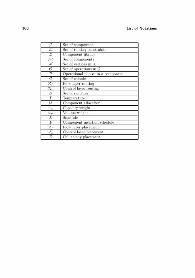
108 List of Notations

J Set of compoundsK Set of routing constraintsL Component libraryM Set of componentsN Set of vertices in AO Set of operations in GP Operational phases in a componentQ Set of coloniesRf Flow layer routingRc Control layer routingS Set of switchesT TemperatureU Component allocationwc Capacity weightwv Volume weightX ScheduleY Component insertion scheduleZf Flow layer placementZc Control layer placementZ Cell colony placement

Bibliography

[1] Affymetrix Inc. http://www.affymetrix.com/.

[2] Agilent Technologies. http://www.home.agilent.com/.

[3] AutoCAD Products. http://usa.autodesk.com/autocad-products/.

[4] Biochips: A Global Strategic Business Report.http://www.strategyr.com/Biochips_Market_Report.asp.

[5] Caliper Life Sciences Inc. http://www.caliperls.com/.

[6] Fluidigm: Chips and Kits. http://www.fluidigm.com/chips-kits.html.

[7] Fluidigm Corporation. http://www.fluidigm.com/.

[8] GE Healthcare Ltd. http://www.gehealthcare.com/.

[9] Illumina, Inc. http://www.illumina.com/.

[10] International Technology Roadmap for Semiconductors 2011 Edition.http://www.itrs.net/Links/2011ITRS/2011Chapters/2011SysDrivers.pdf.

[11] ISI Web of Science, search for topic “microfluidic”.http://www.isiknowledge.com.

[12] KNI Microfluidic Foundry - CalTech. http://www.kni.caltech.edu/foundry/.

[13] Life Technologies Corporation. http://www.lifetechnologies.com/.

[14] mLSI Biochips. https://sites.google.com/site/mlsibiochips/.

[15] Stanford Microfluidic Foundry. http://www.stanford.edu/group/foundry/.

110 BIBLIOGRAPHY

[16] Stephen Quake’s Group at Stanford University.http://thebigone.stanford.edu/.

[17] United States Patent and Trademark office, search issued patents for “mi-crofluidic” in title or abstract. http://patft.uspto.gov.

[18] Verinata Health. http://www.verinata.com/.

[19] A. M. Amin, M. Thottethodi, T. N. Vijaykumar, S. Wereley, and S. C.Jacobson. Aquacore: A programmable architecture for microfluidics. InProceedings of the 34th annual international symposium on Computer ar-chitecture, pages 254–265, 2007.

[20] A. M. Amin, M. Thottethodi, T. N. Vijaykumar, S. Wereley, and S. C.Jacobson. Automatic volume management for programmable microfluidics.In Proceedings of the 2008 ACM SIGPLAN conference on Programminglanguage design and implementation, 2008.

[21] N. Amin, W. Thies, and S. Amarasinghe. Computer-aided design for mi-crofluidic chips based on multilayer soft lithography. In Proceedings of theIEEE International Conference on Computer Design, 2009.

[22] V. Ananthanarayanan and W. Thies. Biocoder: A programming languagefor standardizing and automating biology protocols. Journal of BiologicalEngineering, 4(13), 2010.

[23] I. E. Araci and S. R. Quake. Microfluidic very large scale integration (mvlsi)with integrated micromechanical valves. Lab Chip, 12:2830–2806, 2012.

[24] K. Chakrabarty and T. Xu. Digital Microfluidic Biochips: Design Automa-tion and Optimization. CRC Press, Boca Raton, FL, 2010.

[25] H. Chou, M. Unger, and S.R. Quake. A microfabricated rotary pump.Biomedical Microdevices, 3, 2001.

[26] P. Coussy and A. Morawiec. High-level synthesis: From algorithm to digitalcircuit. Springer, 2008.

[27] P. S. Dittrich and A. Manz. Lab-on-a-chip: microfluidics in drug discovery.Nature Reviews, Drug Discovery, 5:210–218, 2006.

[28] J. El-Ali, P. K. Sorger, and K. F. Jensen. Cells on chips. Nature, 442:403–411, 2006.

[29] C. D. Chin et. al. Microfluidics-based diagnostics of infectious diseases inthe developing world. Nature Medicine, 17:1015–1019, 2011.

BIBLIOGRAPHY 111

[30] S. Einav et. al. Discovery of a hepatitis c target and its pharmacologicalinhibitors by microfluidic affinity analysis. Nature Biotechnology, 12:1019–1027, 2008.

[31] R. B. Fair. Digital microfluidics: is a true lab-on-a-chip possible? Microflu-idics and Nanofluidics, 3(3):245–281, 2007.

[32] H. C. Fan, Y. J. Blumenfeld, U. Chitkara, L. Hudgins, and S. R. Quake.Noninvasive diagnosis of fetal aneuploidy by shotgun sequencing dna frommaternal blood. Proceedings of the National Academy of Sciences USA,105(42):16266–16271, 2008.

[33] C. Fang, Y. Wang, N. T. Vu, W. Lin, Y. Hsieh, L. Rubbi, M. E. Phelps,M. Mueschen, Y. Kim, A. F. Chatziioannou, H. Tseng, and T. G. Grae-ber. Integrated microfluidic and imaging platform for a kinase activityradioassay to analyze minute patient cancer samples. Cancer Research,70(21):8299–8308, November 2010.

[34] F. Glover and M.Laguna. Tabu Search. Kluwer Academic Publishers, 1997.

[35] C. L. Hansen, M. O. A. Sommer, and S. R. Quake. Systematic investigationof protein phase behavior with a microfluidic formulator. Proceedings of theNational Academy of Sciences USA, 101(40):14431–14436, 2004.

[36] D. J. Harrison, K. Fluri, K. Seiler, Z. Fan, C. S. Effenhauser, and A. Manz.Micromachining a miniaturized capillary electrophoresis-based chemicalanalysis system on a chip. Science, 261:895–897, 1993.

[37] A. Hertz and D. Werra. Using Tabu search techniques for graph coloring.Journal of Computing, 39:345–351, 1987.

[38] J. W. Hong, Y. Chen, W. F. Anderson, and S. R. Quake. Molecular biologyon a microfluidic chip. Journal of Physics: Condensed Matter, 18(18):691–701, 2006.

[39] J. W. Hong and S. R. Quake. Integrated nanoliter systems. Nature Biotech-nology, 21:1179–1183, 2003.

[40] J. W. Hong, V. Studer, G. Hang, W. F. Anderson, and S. R. Quake. Ananoliter-scale nucleic acid processor with parallel architecture. NatureBiotechnology, 22(4):435–439, 2004.

[41] D. Karger, R. Motwani, and M. Sudan. Approximate graph coloring bysemidefinite programming. Journal of the ACM (JACM), 45:246–265, 1998.

[42] M. E. Kempner and R. A. Felder. A review of cell culture automation. TheJournal of the Association for Laboratory Automation (JALA), 7(2):56–62,2002.

112 BIBLIOGRAPHY

[43] I. Klammer, A. Buchenauer, H. Fassbender, R. Schlierf, G. Dura,W. Mokwa, and U. Schnakenberg. Numerical analysis and characterizationof bionic valves for microfluidic pdms-based systems. Journal of Microme-chanics and Microengineering, 17(7):S122–S127, 2007.

[44] M. F. Kramer and D. M. Coen. Enzymatic amplification of dna by pcr:Standard procedures and optimization. Current Protocols in MolecularBiology), pages 15.1.1–15.1.14, 2001.

[45] K. Kuchcinski. Constraints-driven scheduling and resource assignment.ACM Transactions on Design Automation of Electronic Systems (TO-DAES), 8(3):355–383, 2003.

[46] H. P. Le. Progress and trends in ink-jet printing technology. Journal ofImaging Science and Technology, 42:49–62, 1998.

[47] C. C. Lee, A. Elizarov, C. J. Shu, Y. S. Shin, and A. N. Dooley. Multistepsynthesis of a radiolabeled imaging probe using integrated microfluidics.Science, 310:1793–1796, 2005.

[48] A. Lim, Y. Zhu, and Q. Lou. Heuristic methods for graph coloring problems.In ACM symposium on Applied Computing, pages 933–939, 2005.

[49] Y. C. Lim, A. Z. Kouzani, and W. Duan. Lab-on-a-chip: a componentview. Journal of microsystems technology, 16(12), December 2010.

[50] H. T. G. Lintel. A piezoelectric micropump based on micromachining ofsilicon. Sensors and Actuators, 15(2):153–167, 1988.

[51] J. Liu, C. Hansen, and S. R. Quake. Solving the “world-to-chip” interfaceproblem with a microfluidic matrix. Analytical Chemistry, 75(18):4718–4723, 2003.

[52] A. Manz, N. Graber, and H. M. Widmerl. Miniaturized total chemical anal-ysis systems: A novel concept for chemical sensing. Sensors and ActuatorsB: Chemical, 1:244–248, 1990.

[53] J. S. Marcus, W. F. Anderson, and S. R. Quake. Microfluidic single-cellmrna isolation and analysis. Analytical Chemistry, 78(9):3084–3089, 2006.

[54] D. Mark, S. Haeberle, G. Roth, F. Stetten, and R. Zengerle. Microflu-idic lab-on-a-chip platforms: requirements, characteristics and applications.Chem. Soc. Rev., 39:1153–1182, 2010.

[55] J. Melin and S. Quake. Microfluidic large-scale integration: The evolutionof design rules for biological automation. Annual Reviews in Biophysicsand Biomolecular Structure, 36:213–231, 2007.

BIBLIOGRAPHY 113

[56] G. D. Micheli. Synthesis and optimization of digital circuits. McGraw-Hill,New York, 1994.

[57] W. H. Minhass, P. Pop, and J. Madsen. Application-specific architecturalsynthesis for the flow-based microfluidic large-scale integration biochips.IEEE Transactions on Computer-Aided Design of Integrated Circuits andSystems (preparing for submission).

[58] W. H. Minhass, P. Pop, and J. Madsen. System-level modeling and appli-cation mapping on the flow-based microfluidic very large scale integrationbiochips. IEEE Transactions on Very Large Scale Integration (VLSI) Sys-tems (preparing for submission).

[59] W. H. Minhass, P. Pop, and J. Madsen. System-level modeling and syn-thesis of flow-based microfluidic biochips. In Proc. of the InternationalConference on Compilers, Architectures and Synthesis of Embedded Sys-tems (CASES), 2011.

[60] W. H. Minhass, P. Pop, and J. Madsen. Synthesis of Biochemical Applica-tions on Flow-Based Microfluidic Biochips using Constraint Programming.In Proc. of the IEEE Symposium on Design, Test, Integration and Packag-ing of MEMS/MOEMS (DTIP), pages 37–41, 2012.

[61] W. H. Minhass, P. Pop, J. Madsen, and F. S. Blaga. Architectural synthesisof flow-based microfluidic large-scale integration biochips. In Proceedingsof the International Conference on Compilers, Architectures and Synthesisof Embedded Systems (CASES), pages 181–190, 2012.

[62] W. H. Minhass, P. Pop, J. Madsen, M. Hemmingsen, and M. Dufva.System-level modeling and simulation of the cell culture microfluidicbiochip ProCell. In Proc. of the IEEE Symposium on Design, Test, In-tegration and Packaging of MEMS/MOEMS (DTIP), pages 91–98, 2010.

[63] W. H. Minhass, P. Pop, J. Madsen, M. Hemmingsen, P. Skafte-Pedersen,and M. Dufva. Cell Culture Microfluidic Biochips: Experimental Through-put Maximization. In Proc. of the IEEE International Conference on Bioin-formatics and Biomedical Engineering (iCBBE), 2011.

[64] W. H. Minhass, P. Pop, J. Madsen, and T. Ho. Control synthesis andpin count minimization for the flow-based microfluidic large-scale integra-tion biochips. Journal on Emerging Technologies in Computing Systems(preparing for submission).

[65] W. H. Minhass, P. Pop, J. Madsen, and T. Ho. Control Synthesis for theFlow-Based Microfluidic Large-Scale Integration Biochips. In Proc. of theAsia and South Pacific Design Automation Conference (ASP-DAC), 2013.

114 BIBLIOGRAPHY

[66] J. M. Perkel. Microfluidics - bringing new things to life science. Science,November 2008.

[67] M. G. Pollack, A. D. Shenderov, and R. B. Fair. Electrowetting-basedactuation of droplets for integrated microfluidics. Lab Chip Journal, 2:96–101, 2002.

[68] P. Pop, E. Maftei, and J. Madsen. Recent research and emerging challengesin the system-level design of digital microfluidic biochips. In Proc. of theIEEE International SOC Conference (SOCC), 2011.

[69] S. M. Sait and H. Youssef. VLSI physical design automation: theory andpractice. World Scientific Publishing Co. Pte. Ltd., 1999.

[70] M. F. Schmidt, W. H. Minhass, P. Pop, and J. Madsen. Modeling and simu-lation framework for flow-based microfluidic biochips. In Proc. of the IEEESymposium on Design, Test, Integration and Packaging of MEMS/MOEMS(DTIP), 2013.

[71] C. Schulte, G. Tack, and M. Z. Lagerkvist. Modeling and programmingwith gecode. http://www.gecode.org/.

[72] S. Shoji, M. Esashi, and T. Matsuo. Prototype miniature blood gas analyserfabricated on a silicon wafer. Sensors and Actuators, 14(2):101–107, 1988.

[73] J. Siegrist, M. Amasia, N. Singh, D. Banerjee, and M. Madou. Numericalmodeling and experimental validation of uniform microchamber filling incentrifugal microfluidics. Lab Chip, 10:876–886, 2010.

[74] O. Sinnen. Task Scheduling for Parallel Systems. John Wiley & Sons Inc.,Hoboken, New Jersey, 2007.

[75] G. Sittampalam, S. Kahl, and W. Janzen. High-throughput screening:advances in assay technologies. Curr Opin Chem Biology, 1(3):384–391,1997.

[76] P. Skafte-Pedersen, M. Hemmingsen, D. Sabourin, F. S. Blaga, H. Bruus,and M. Dufva. A self-contained, programmable microfluidic cell culturesystem with real-time microscopy access. Biomed Microdevices, 14(2):385–399, 2012.

[77] A. Stacey and G. Stacey. Routine quality control testing of cell cultures,Antiviral Methods and Protocols (3). Springer, 2000.

[78] F. Su and K. Chakrabarty. High-level synthesis of digital microfluidicbiochips. Journal on Emerging Technologies in Computing Systems, 3(4),January 2008.

BIBLIOGRAPHY 115

[79] F. Su, S. Ozev, and K. Chakrabarty. Concurrent testing of droplet-basedmicrofluidic systems for multiplexed biomedical assays. In Proceedings ofthe International Test Conference (ITC), pages 883–892, 2004.

[80] S. C. Terry, J. H. Jerman, and J. B. Angell. A gas chromatographic airanalyzer fabricated on a silicon wafer. IEEE Transactions on ElectronDevices, 26(12):1880–1886, 1979.

[81] W. B. Thies. Programmable microfluidics. presented at Stanford University,October 2007.

[82] T. Thorsen, S. J. Maerki, and S. R. Quake. Microfluidic large-scale inte-gration. Science, 298(5593):580–584, October 2002.

[83] D. Ullman. Np-complete scheduling problems. Journal of Computing Sys-tem Science, 10:384–393, 1975.

[84] D. Ullman. NP-complete scheduling problems. Journal of Computing Sys-tem Science, 10:384–393, 1975.

[85] J. P. Urbanski, W. Thies, C. Rhodes, S. Amarasinghe, and T. Thorsen.Digital microfluidics using soft lithography. Lab Chip, 6:96–104, 2006.

[86] V. T. Vanchikov. Special form of laminar liquid flow in hydraulic devices.Russian Engineering Research, 28(9):854–855, 2008.

[87] G. M. Whitesides. The origins and the future of microfluidics. Nature,442:368–373, July 2006.

[88] Y. Zhao and K. Chakrabarty. Cross-contamination avoidance for dropletrouting in digital microfluidic biochips. IEEE Transactions on Computer-Aided Design of Integrated Circuits and Systems, 31:817–830, June 2012.