System Identification on Alstom ECO100 Wind Turbine

Carlo E. Carcangiu Alstom Wind

78, Roc Boronat 08005-Barcelona, Spain carlo-enrico.carcangiu @power.alstom.com

Stoyan Kanev ECN Wind Energy

P.O. Box 1, 1175LE Petten, the Netherlands

kanev@ecn.nl

Michele Rossetti Alstom Wind

78, Roc Boronat 08005-Barcelona, Spain

michele.rossetti @power.alstom.com

Iciar Font Balaguer Alstom Wind

78, Roc Boronat 08005-Barcelona, Spain

iciar.font @power.alstom.com

ABSTRACT

Control algorithms for wind turbines are traditionally designed on the basis of

(linearized) dynamic models. On the accuracy of such models depends hence the

performance of the control, and validating the dynamic models is an essential

requirement for achieving the optimum design. The aim of this work is to identify, at

different wind speeds, the dynamic model of a wind turbine in operation.

Experimental modal analysis is the selected technique for system identification, and

band-limited pseudo-random excitation signals are summed to the controlled inputs

of the wind turbine system.

Fairly good match is found in frequency and damping ratio for a frequency range up

to 1 Hz. The time domain validation indicates in all cases reasonable model quality.

The frequency domain comparison carried out for selected wind speeds shows close

overlap around the first tower fore-aft and side-to-side frequencies, even though

some discrepancies are found at first drive train frequencies.

Keywords: System Identification, Experimental Modal Analysis, PRBS, Wind

Turbine Control.

1 INTRODUCTION

Control algorithms for wind turbines are traditionally designed on the basis of

(linearized) dynamic models. On the accuracy of such models depends hence the

performance of the control, and validating the dynamic models is an essential

requirement for achieving the optimum design. The aim of this work is to identify, at

different wind speeds, the dynamic model of a wind turbine.

Experimental modal analysis (EMA) system identification has been applied on the

Alstom Eco100 Wind turbine in order to extract modal information at different

operational conditions. Proper band-limited pseudo-random binary excitation signals

(PRBS) have been carefully arranged to avoid the induction of undesired significant

loads on the tower and rotor, taking also into account the constraints of the

actuators. Experimental modeling is an orthogonal approach to “first principles”

physical modeling, where the phenomena observed in reality are modeled by using

measured data from the operational wind turbine. To this end, system identification

techniques are used to fit the parameters of a suitable mathematical model to the

measured data as good as possible.

For wind turbine applications, experimental modeling has only received limited

attention in the literature. The application of “exciter methods”, where rather

unrealistic direct and measurable excitation on several points on the blades is

assumed, was investigated by Bialasiewicz [1]. Recently, research on modal

analysis was performed within the framework of the European research project

“STABCON” - Stability and control of large wind turbines'', where both simulation

studies and experimental results were included [2][3]. The simulation studies are

based on blade excitations that are difficult to perform in practice. More realistic

excitation signals were investigated at Risø National Laboratory, by using the blade

pitch and generator to excite with harmonic signals the first two tower bending

modes, even though the measurement of the decaying response was proved to be

unsuitable for an accurate estimation of the damping [3]. The identification of open-

loop drive train dynamics from closed-loop experimental measurements on a fixed-

pitch variable-speed wind turbine is presented in [4], for control algorithm design

purposes.

Because the experimental modeling is based on data collected from a wind turbine

during operation, i.e. with the controller operating, closed-loop system identification

must be applied. Prior to the current work, a detailed review has been hence carried

out of the available closed-loop identification (CLID) approaches to wind turbine

model identification, listed below:

Direct method [5],

Indirect method [5],

Joint Input/output method [5],

Closed-loop instrumental variable method [6],

Tailor made instrumental variable method [7],

Closed-loop N4SID subspace identification [8],

Parsimonious subspace identification method (PARSIM) [9],

Subspace identification based on output predictions (SSARX) [10].

Initial studies using simulation data from both linear and nonlinear aeroelastic

simulations have indicated the methods Direct, SSARX and PARSIM as most

promising for wind turbine applications, with the Direct method often outperforming

the other methods. For that reason, and for the sake of space limitation, only the

Direct method is summarized in Section 2.1.

In order to identify accurate (i.e. unbiased) input-output models using the above-

mentioned system identification methods, it is necessary that the inputs are

additionally excited by signals that are uncorrelated with the wind. How this can be

achieved without introducing unacceptable additional loads will be discussed in

Section 2.2. Moreover, special attention has also been paid on data-driven model

validation, for which purpose several techniques have been developed and

summarized in Section 2.3. A number of model validation methods are presented in

Section 2.4. The experimental tests results are included Section 3, splitting tower

and drive train modes.

2 METHODOLOGY

2.1 Direct method for closed-loop identification

In the direct method [5], a so-called prediction error model identification is applied to

the data, collected while the wind turbine operates in closed-loop. The starting point

of the method is the selection of a suitable model structure. For wind turbine

applications, a simple auto-regressive-with-exogenous-input (ARX) model is proved

to be sufficient. The ARX model has the following form

)()().()(.)( kekupBkypA += (1)

where lRky ∈)( is a generalized output vector, mRku ∈)( is the input vector,

lRke ∈)( is some unknown generalized disturbance signal representing the influence

of the wind on the output measurements, k is the moment of time, and lxlRPA ∈)(

and lxmRPB ∈)( are matrix polynomials dependent on the unknown parameter P

[ ]nbna

nb

nb

na

na

BBAAP

qBqBqBBPB

qAqAqAIPA

,,,

,)(

,)(

,0,1

2

2

1

10

2

2

1

1

KK

L

L

=

++++=

++++=−−−

−−−

(2)

Above, 1−q denotes the backward time shift operator, i.e. )1()(1 −=− kykyq .

The goal is to estimate the model parameters p given input/output data N

kkyku

1)(),( = .

This is achieved in the following way. Given the ARX model structure, the one step

ahead predictor for the output vector is formed

)])(,),(),(),1(([)(

),(.)(ˆ

nbkukunakykyveck

kPky

−−−−−=

=

KKϕ

ϕ (3)

where )(Mvec is the “vectorization” operator which stacks the columns of a matrix

into one vector. This predictor model is used for constructing the prediction error

)()()(ˆ)()( kPkykykyk ϕε −=−= (4)

To estimate the unknown parameter matrix P , the following prediction error criterion

is minimized with respect to P

∑

=

=N

k

kN

PV1

2

2)(

2

11)( ε

(5)

An analytical expression can be obtained for the parameter matrix P that minimizes

the prediction error criterion by using the fact that for given matrices of appropriate

dimensions, the following expression holds

).().(.. YvecXZZYX T ⊗= (6)

hence

( )∑

∑

=

=

⊗−⊗=

⊗−∂

∂=

∂

∂

N

k

TTT

N

k

T

PvecIkkyIkN

PvecIkkyNPvec

Pvec

PV

1

1

2

2

)())(()())((2

11

)())(()(2

11

)(

)(

)(

ϕϕ

ϕ (7)

giving

⊗

⊗⊗

=

∑∑=

−

=

N

k

TTN

k

TTT kyIkN

IkIkN

Pvec

1

1

1

)())((1

))(())((1

)(

ϕϕϕ (8)

The identified ARX model is then parameterized by this optimal parameter matrix P .

It can be theoretically shown that the identified model is unbiased under reasonable

assumptions [5].

2.2 Excitation signal design

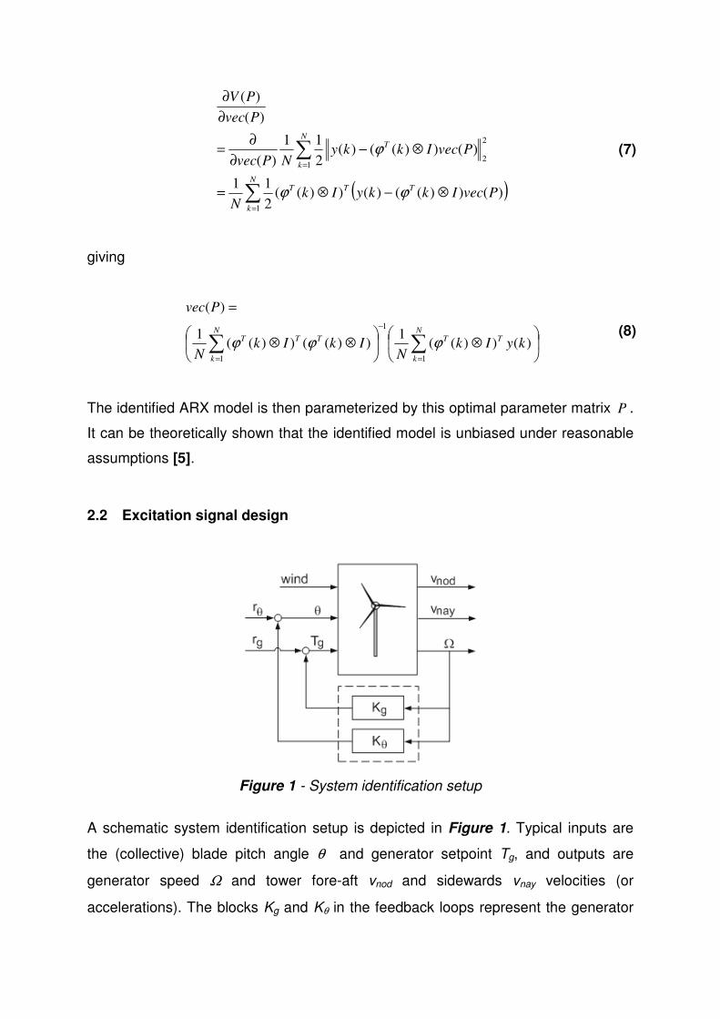
Figure 1 - System identification setup

A schematic system identification setup is depicted in Figure 1. Typical inputs are

the (collective) blade pitch angle θ and generator setpoint Tg, and outputs are

generator speed Ω and tower fore-aft vnod and sidewards vnay velocities (or

accelerations). The blocks Kg and Kθ in the feedback loops represent the generator

and the pitch controllers, respectively, which are not required in the Direct

identification methods, presented in Section 2.1. Time series of these typical inputs

and outputs allow the identification of the transfer functions from θ to vnod, from Tg to

Ω, and from Tg to vnay, from which the tower fore-aft, tower side-to-side and drive

train dynamics can be analyzed.

The frequency range where the models can be accurately identified depends on the

bandwidth of the excitation signals: rθ (on the blade pitch) and/or rg (on the

generator). When the frequency and damping of the first tower mode need to be

identified, the bandwidth should at least include the expected first tower frequency.

When the first drive-train mode is needed, the excitation bandwidth must at least

include the first drive-train frequency. Hence, the proper choice of excitation signals

is key-important for achieving informative experiment under reasonable amount of

excitation.

Two opposite objectives exist indeed, and a trade-off should be made. On the one

hand, a good excitation for system identification can be achieved by choosing a high

energy excitation signal with wide flat spectrum. On the other hand, the system

limitations (such as hardware limits, loads, etc.) impose the use of low-energy,

narrow bandwidth excitation. The design of excitation signals should therefore

prescribe that (a) the signals remain within the hardware limits, (b) the additional

loads are as small as possible, and (c) the dynamic models are still accurately

identified.

For the considered wind turbine specifically, the excitation signals rθ and rg have

been designed in such a way, that no unacceptable loads are induced, the excited

pitch demand has acceptable speed and acceleration, and the electric power

remains within acceptable limits. To this end,

the pitch excitation signal rθ is designed as a pseudo-random binary signal

(PRBS) with amplitude of 0.5 degrees, filtered with a low-pass FIR filter with

cutoff frequency of 1 Hz, and an elliptic bandstop filter with 20 dB reduction, 1 dB

ripple, and stop-band of 30% around the expected first tower frequency (0.32

Hz). In this way, the pitch excitation does not excite the region around the

expected first tower frequency, as well as frequencies above 1 Hz.

the generator excitation signal rg is also designed as PRBS signal, but

uncorrelated with the one used for pitch excitation, and with an amplitude of 3%

of the rated signal, filtered with a lowpass FIR filter with cutoff frequency of 2 Hz,

so that the excitation is concentrated in the frequency region up to 2 Hz.

Simulations made with an aeroelastic code have demonstrated that these excitations

do not introduce significant increment in loads.

2.3 Modal parameters estimation

Once a model of the wind turbine is identified, there are different ways to extract

modal parameters, such as the first tower and drive-train frequencies and damping.

One way to do that is by performing model reduction on the identified mode, to

reduce the model order, such as there is only one mode in a specified interval of

interest where the frequency is expected to lie. For the considered wind turbine, the

selected interval is [0.25, 0.40] Hz for the tower, and [0.7, 1] Hz for the drive train.

The retained mode is the mode with the largest participation factor. The frequency

and damping of this mode are then selected from the reduced system.

2.4 Model validation methods

Model validation is the process of deciding whether an identified model is reliable

and suitable for the purposes for which it has been created.

The following model validation methods have been used to check the accuracy of

the identified model:

Variance-accounted-for (VAF): this is a model validation index often used with

subspace identification methods. Given the measured output )(ky and the output

predicted by the one step ahead predictor )(ˆ ky , the VAF criterion is defied as

u

yyVAFσ

σ ε−= 1)ˆ,(

(9)

Where yσ is the variance of the signal )(ky , and εσ the variance of the

prediction error ε . It is expressed in percentage. A VAF above the 95% is usually

considered to represent a very accurate model.

Prediction error cost (PEC): this is the value of the prediction error cost function,

defined above. The smaller the value, the better the model accuracy.

Auto-correlation index ( εixR ): when a consistent model estimate is made, the

prediction error ε should be a white process, so that its auto-correlation function

)(τεR should be small for non-zero τ , whereτ denotes the discrete time step.

For a given confidence level α (e.g. %99=α ), a bound )(αεbnd

R can be derived

such that for an accurate model the inequality )()( ατ εεbndRR ≤ should hold for all

1≥τ . The index εixR is then computed as the square sum of the distance between

each value of the correlation function )(τεR and the bound )(αεbnd

R , where only

the values outside the bound are used.

Cross-correlation index ( u

ixRε ): in the closed-loop situation the prediction error will

be correlated with future values of the input, but should be uncorrelated with past

inputs when the model is consistent. The cross-correlation function )(τεuR should

then be limited in absolute value for 1≥τ . The index u

ixRε is computed similarly to

εixR .

It is important to point out that the data set used for validating the models should be

different from the data used for obtaining the model, as otherwise wrong conclusions

could be drawn. When the data length is short, a rule of thumb is to use two thirds of

the data for identification, and the remaining one third for validation.

3 RESULTS

3.1 Preliminary simulations

Time domain closed-loop system identification methods (CLID) are applied to both

simulations, used to verify loads and to check identification methodologies, as well

as to measurement data from an Alstom ECO100 wind turbine using PRBS signals

as defined in Section 2.2.

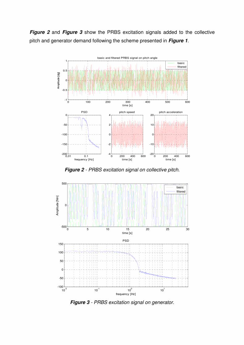
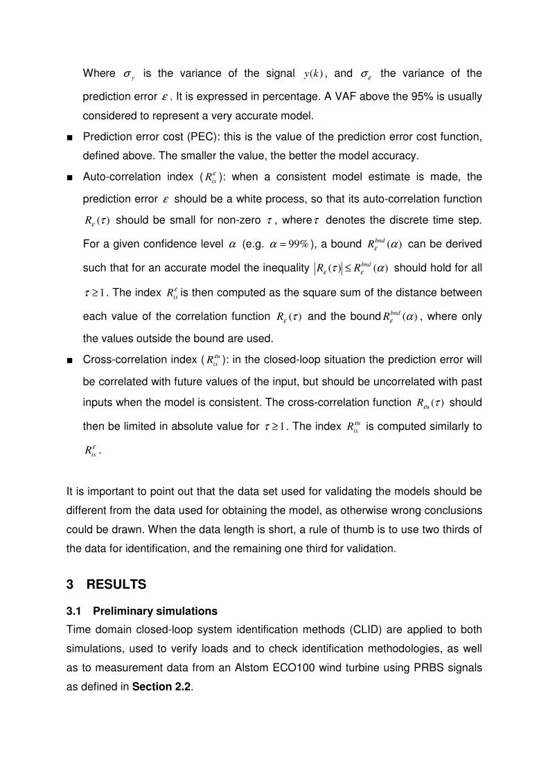
Figure 2 and Figure 3 show the PRBS excitation signals added to the collective

pitch and generator demand following the scheme presented in Figure 1.

0 100 200 300 400 500 600-1

-0.5

0

0.5

1basic and filtered PRBS signal on pitch angle

Am

plitu

de [dg

]

time [s]

0,01 0.1-200

-150

-100

-50

0PSD

frequency [Hz]0 200 400 600

-4

-2

0

2

4pitch speed

time [s]0 200 400 600

-20

-10

0

10

20pitch acceleration

time [s]

basic

filtered

Figure 2 - PRBS excitation signal on collective pitch.

0 5 10 15 20 25 30-500

0

500

Am

plitu

de [

Nm

]

time [s]

basic

filtered

10

-210

-110

010

1-100

-50

0

50

100

150PSD

frequency [Hz]

Figure 3 - PRBS excitation signal on generator.

As explained in Section 2, closed-loop identification techniques are used to identify

open loop models. Given the identified models, the corresponding frequency and

damping of the first tower fore-aft and side-to-side mode and the first drive train

mode of the open-loop wind turbine can be computed at different wind speeds. Time

and frequency validation methods are used to evaluate each method.

As first step, closed-loop identification techniques are applied to (excited)

input/output data from aeroelastic simulations. Simulations show that no significant

loads were induced on the turbine, the excited pitch demand had acceptable speed

and acceleration, and the electric power remained within acceptable limits.

As second step, studies on the closed-loop identification methods are carried out

using simulation data. Since no information about the controller and the exact

excitation signals used (rө and rg) is provided, the Direct, SSARX and PARSIM

appear to be the most promising methods for wind turbine applications.

3.2 The measurement campaign

The same closed-loop identification techniques are applied using real (excited)

input/output data collected from measurements on Alstom ECO100 3MW wind

turbine. The measurement campaign was performed at below rated wind speeds,

varying between 4 and 8 m/s. The control inputs, collective pitch demand and

generator demand, have been simultaneously excited with the PRBS signals in order

to obtain the transfer functions from these inputs to the outputs generator speed and

tower top fore-aft and sideward velocities. The input/output measurement data

collected are summarized in Table 1.

Table 1 - Signals stored from the real wind turbine

Generator speed Ω rpm

Tower top fore-aft acceleration vfa m/s2

Tower top fore-aft acceleration vsd m/s2

Excited blade pitch angle demand ө deg

Excited generator torque Tg Nm

Wind speed at nacelle Vnac m/s

Experience shows that working with tower top velocities improves the quality of the

identified models around the first tower modes. Hence, for the estimation of the

tower modes, the outputs vfa and vsd are integrated to velocities vnod and vnay.

Four measurement time series are selected, each taken during partial load

operation. Due to the fact that each of these four measurements cases contains

some irrelevant information from the identification point of view, they have been

concatenated. As indicated in the Table 2, Test 1 and 2 have the same mean wind

speed. Hence, Test 1 data can be used for model identification, while Test 2 can be

used as validation data at 4.5 m/s. The same holds for Test 3 and 4, where the mean

wind speed is 6.3 m/s.

Table 2 - Measurement time series from the real wind turbine

Test case Data length Mean (Vnac) Purpose

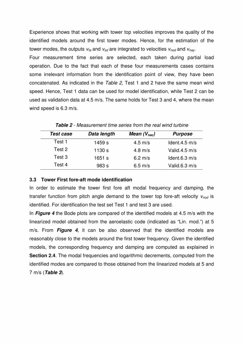
Test 1 1459 s 4.5 m/s Ident.4.5 m/s Test 2 1130 s 4.8 m/s Valid.4.5 m/s Test 3 1651 s 6.2 m/s Ident.6.3 m/s Test 4 983 s 6.5 m/s Valid.6.3 m/s

3.3 Tower First fore-aft mode identification

In order to estimate the tower first fore aft modal frequency and damping, the

transfer function from pitch angle demand to the tower top fore-aft velocity vnod is

identified. For identification the test set Test 1 and test 3 are used.

In Figure 4 the Bode plots are compared of the identified models at 4.5 m/s with the

linearized model obtained from the aeroelastic code (indicated as “Lin. mod.”) at 5

m/s. From Figure 4, it can be also observed that the identified models are

reasonably close to the models around the first tower frequency. Given the identified

models, the corresponding frequency and damping are computed as explained in

Section 2.4. The modal frequencies and logarithmic decrements, computed from the

identified modes are compared to those obtained from the linearized models at 5 and

7 m/s (Table 3).

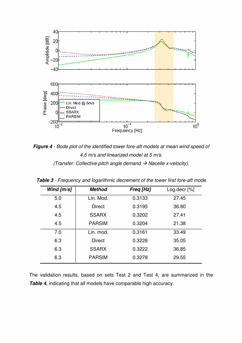
Figure 4 - Bode plot of the identified tower fore-aft models at mean wind speed of

4.5 m/s and linearized model at 5 m/s.

(Transfer: Collective pitch angle demand Nacelle x-velocity).

Table 3 - Frequency and logarithmic decrement of the tower first fore-aft mode

Wind [m/s] Method Freq [Hz] Log.decr [%]

5.0

4.5

4.5

4.5

Lin. Mod.

Direct

SSARX

PARSIM

0.3133

0.3195

0.3202

0.3204

27.45

36.80

27.41

21.38

7.0

6.3

6.3

6.3

Lin. mod.

Direct

SSARX

PARSIM

0.3161

0.3228

0.3222

0.3278

33.49

35.05

36.85

29.55

The validation results, based on sets Test 2 and Test 4, are summarized in the

Table 4, indicating that all models have comparable high accuracy.

Table 4 - Validation results for identified models of the tower first fore-aft.

Wind

[m/s]

Method VAF PEC

(x10-5)

εixR u

ixRε (x10-2)

4.5

4.5

4.5

Direct

SSARX

PARSIM

97.43

97.26

95.99

3.592

3.706

4.487

0.7129

2.744

2.517

1.2

1.344

6.346

6.3

6.3

6.3

Direct

SSARX

PARSIM

97.36

97.36

97.18

4.684

4.68

4.841

0.7638

0.6674

0.8528

3.59

3.843

4.164

3.4 Tower First side to side mode identification

Similarly, to estimate the tower first side to side modal frequency and damping, the

transfer function from generator demand Tg to the tower top side to side velocity vnay

is identified. In Figure 5 the bode plots of the identified models at 6.3 m/s with

linearized model at 7 m/s are shown.

Figure 5 - Bode plot of the identified tower side to side models at mean wind speed

of 6.3 m/s and linearized model at 7 m/s.

(Transfer: Generator torque Nacelle y-velocity).

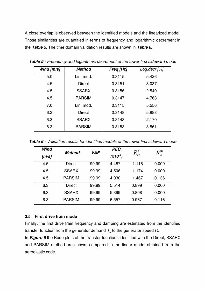
A close overlap is observed between the identified models and the linearized model.

Those similarities are quantified in terms of frequency and logarithmic decrement in

the Table 5. The time domain validation results are shown in Table 6.

Table 5 - Frequency and logarithmic decrement of the tower first sideward mode

Wind [m/s] Method Freq [Hz] Log.decr [%]

5.0

4.5

4.5

4.5

Lin. mod.

Direct

SSARX

PARSIM

0.3115

0.3151

0.3156

0.3147

5.426

3.037

2.549

4.763

7.0

6.3

6.3

6.3

Lin. mod.

Direct

SSARX

PARSIM

0.3115

0.3148

0.3143

0.3153

5.556

5.883

2.170

3.861

Table 6 - Validation results for identified models of the tower first sideward mode

Wind

[m/s] Method VAF

PEC

(x10-5)

εixR

u

ixRε

4.5

4.5

4.5

Direct

SSARX

PARSIM

99.99

99.99

99.99

4.487

4.506

4.030

1.118

1.174

1.467

0.009

0.000

0.136

6.3

6.3

6.3

Direct

SSARX

PARSIM

99.99

99.99

99.99

5.514

5.399

6.557

0.899

0.808

0.967

0.000

0.000

0.116

3.5 First drive train mode

Finally, the first drive train frequency and damping are estimated from the identified

transfer function from the generator demand Tg to the generator speed Ω.

In Figure 6 the Bode plots of the transfer functions identified with the Direct, SSARX

and PARSIM method are shown, compared to the linear model obtained from the

aeroelastic code.

Figure 6 - Bode plot of identified first drive train models at mean wind speed of 6.3

m/s and linearized model at 7 m/s. (Transfer: Generator torque Generator speed)

As reported in Table 7, the identified drive-train frequency is about 10% higher than

the linearized model. Comparing the linearized model obtained with the aeroelastic

code to the identified model using PARSIM method, a better estimation is obtained.

In any case, the drive train frequency is not clearly evident in the input-output data.

Table 7 - Frequency and logarithmic decrement of the first drive train mode.

Wind

[m/s]

Method Freq [Hz] Log.decr [%]

5.0

4.5

4.5

4.5

Lin. mod.

Direct

SSARX

PARSIM

0.7777

0.8773

0.8780

0.8261

1.304

14.120

16.610

6.877

7.0

6.3

6.3

6.3

Lin. mod.

Direct

SSARX

PARSIM

0.7780

0.8496

0.8534

0.8305

1.642

1.499

1.822

3.857

In contrast with the frequency domain results showed in Table 7, the Time domain

validation methods shows excellent results (Table 8).

Table 8 - Validation results for identified models of the first drive train mode

Wind [m/s]

Method VAF PEC

(x10-3) εixR

u

ixRε

4.5

4.5

4.5

Direct

SSARX

PARSIM

99.98

99.98

99.96

6.797

6.731

10.040

0.070

0.051

0.847

0.732

0.670

0.856

6.3

6.3

6.3

Direct

SSARX

PARSIM

100

100

100

5.970

5.962

6.908

0.240

0.181

0.130

0.100

0.256

0.421

An explanation for those differences could be either that the drive-train frequency is

not well represented in the data due to the presence of a drive-train damping filter

existing in the control or that in reality, the drive train is less flexible than in the

linearized model obtained from the aeroelastic code. Further experiments needs to

be performed to clarify the reasons of such discrepancies.

4 CONCLUSIONS

Theory and results of an innovative experimental system identification method for

estimating modal parameters of a wind turbine in operation is presented.

In the mentioned method, additional excitation signals on the controllable inputs of

the turbine (pitch and/or generator) are needed. These signals are designed in such

a way that accurate models are identified, but preventing the occurrence of extra

loads on the wind turbine. In order to validate the identified open-loop models, both

time-domain validation methods and frequency-domain comparisons to linearized

aeroelastic models are made. After preliminary simulations with aeroelastic models,

an experimental campaign has been carried out on the ECO100 3 MW wind turbine

for different below-rated operational conditions.

Fairly good match is found in frequency and damping ratio for a frequency range up

to 1 Hz. The time domain validation indicates in all cases reasonable model quality.

The frequency domain comparison carried out for selected wind speeds shows close

overlap around the first tower fore-aft and side-to-side frequencies, even though

some discrepancies are found at first drive train frequencies. Further experiments

need to be performed to clarify the exact reason of this divergence by either

increasing the generator excitation amplitude or by de-activating the drive-train filter

in the controller.

The estimated modal parameters can be used for either improving the existing

control loops, for achieving additional functionality by designing new control

strategies for fatigue reduction or for updating the existing FEM and multibody

models.

ACKNOWLEDGEMENTS

This work has been partially performed by ECN Wind Energy within the

SenternNovem long-term research project “SusCon: a new approach to control wind

turbines” (EOSLT02013), and partially within the InVent project-ACC1Ó (CIDEM |

COPCA).

REFERENCES

[1] Bialasiewicz, J. (1995): Advanced System Identification Techniques for Wind

Turbine Structures. Report NREL/TP-442-6930, NREL. Prepared for the 1995

SEM Spring Conference, Grand Rapids, Michigan, USA.

[2] Marrant, B. and T. van Holten (2004): System Identification for the analysis of

aeroelastic stability of wind turbine blades. Proceedings of the European Wind

Conference & Exhibition, pp. 101--105.

[3] Hansen, M.H., K. Thomsen, P. Fuglsang and T. Knudsen (2006): Two methods

for estimating aeroelastic damping of operational wind turbine modes from

experiments. Wind Energy, 9(1--2):179--191.

[4] Novak, P., T. Ekelund, I. Jovik and B. Schmidtbauer (1995): Modeling and

control of variable-speed wind-turbine drive-system dynamics. IEEE Control

Systems, 15(4):28--38.

[5] Ljung, L. (1999): System Identification. Theory for the User. Prentice Hall.

[6] Van den Hof, P. and X. Bombois (2004): System Identification for Control.

Delft Center for Systems and Control, TU-Delft. Lecture notes, Dutch Institute

for Systems and Control (DISC)

[7] Van den Hof, P. and M. Gilson (2001): Closed-loop system identification via a

tailor-made IV method. Proceedings of the 40th Conference on Decision and

Control. Orlando, Florida, pp. 4314--4319

[8] Van Overschee, P. and B. De Moor (1997): Closed-loop Subspace System

Identification. Proceedings of the 36th Conference on Decision and Control.

San Diago, California, USA.

[9] Qin, S. and L. Ljung (2003): Closed-Loop Subspace Identification with

Innovation Estimation. Proceedings of the 13th IFAC Symposium on System

Identification, pp. 887-892.

[10] Ljung, L. and T. McKelvey (1996): Subspace identification from closed loop

data. Signal Processing, 52:209-215.