NASA / TM-2001-211243

System Identification and Pod Method

Applied to Unsteady Aerodynamics

Deman Tang and Denis KholodarDuke University, Durham, North Carolina

Jer-Nan JuangLangley Research Center, Hampton, Virginia

Earl H. Dowell

Duke University, Durham, North Carolina

December 2001

https://ntrs.nasa.gov/search.jsp?R=20020015800 2018-07-15T14:21:23+00:00Z

The NASA STI Program Office ... in Profile

Since its founding, NASA has been dedicated tothe advancement of aeronautics and spacescience. The NASA Scientific and Technical

Information (STI) Program Office plays a keypart in helping NASA maintain this importantrole.

The NASA STI Program Office is operated byLangley Research Center, the lead center forNASA's scientific and technical information. The

NASA STI Program Office provides access to theNASA STI Database, the largest collection ofaeronautical and space science STI in the world.The Program Office is also NASA's institutionalmechanism for disseminating the results of itsresearch and development activities. Theseresults are published by NASA in the NASA STI

Report Series, which includes the followingreport types:

TECHNICAL PUBLICATION. Reports ofcompleted research or a major significantphase of research that present the results ofNASA programs and include extensivedata or theoretical analysis. Includescompilations of significant scientific andtechnical data and information deemed to

be of continuing reference value. NASAcounterpart of peer-reviewed formalprofessional papers, but having lessstringent limitations on manuscript lengthand extent of graphic presentations.

TECHNICAL MEMORANDUM. Scientific

and technical findings that are preliminaryor of specialized interest, e.g., quick releasereports, working papers, andbibliographies that contain minimalannotation. Does not contain extensive

analysis.

CONTRACTOR REPORT. Scientific and

technical findings by NASA-sponsoredcontractors and grantees.

CONFERENCE PUBLICATION. Collected

papers from scientific and technicalconferences, symposia, seminars, or othermeetings sponsored or co-sponsored byNASA.

SPECIAL PUBLICATION. Scientific,

technical, or historical information from

NASA programs, projects, and missions,often concerned with subjects havingsubstantial public interest.

TECHNICAL TRANSLATION. English-language translations of foreign scientificand technical material pertinent to NASA'smission.

Specialized services that complement the STIProgram Office's diverse offerings includecreating custom thesauri, building customizeddatabases, organizing and publishing researchresults ... even providing videos.

For more information about the NASA STI

Program Office, see the following:

• Access the NASA STI Program Home Pageat http://www.sti.nasa.gov

• E-mail your question via the Internet to

help@sti.nasa.gov

• Fax your question to the NASA STI HelpDesk at (301) 621-0134

• Phone the NASA STI Help Desk at(301) 621-0390

Write to:

NASA STI Help Desk

NASA Center for AeroSpace Information7121 Standard Drive

Hanover, MD 21076-1320

NASA / TM-2001-211243

System Identification and Pod MethodApplied to Unsteady Aerodynamics

Deman Tang and Denis KholodarDuke University, Durham, North Carolina

Jer-Nan JuangLangley Research Center, Hampton, Virginia

Earl H. Dowell

Duke University, Durham, North Carolina

National Aeronautics and

Space Administration

Langley Research CenterHampton, Virginia 23681-2199

December 2001

Available from:

NASA Center for AeroSpace Information (CASI)7121 Standard Drive

Hanover, MD 21076-1320

(301) 621-0390

National Technical Information Service (NTIS)

5285 Port Royal Road

Springfield, VA 22161-2171

(703) 605-6000

SYSTEM IDENTIFICATION AND POD METHOD

APPLIED TO UNSTEADY AERODYNAMICS

Deman Tang * and Denis t(holodar t

D%l_;e U%i_J_;.rsif:_j, D'_._,'_'haTr_,,No<[:h Ca,<oS'_m. 27708-0300

Jer-Nan Juang ;

ArASA L¢.t'r_gl_<g _esea,rch C_m,f:e'r', H(1.'mi)f:or?_, _(4 23651

Earl H. Dowell

D%ke Ur:,ive'_+si_:g, D,_l,vha'm,, North Ca?+oS'rm 27708-0300

ABSTRACT

The representation of unsteady aerodynamic flow fields in t.erms of global aerodynamic modes

has proven t,o be a usdhl met.hod for reducing the size of the aerodynamic model over those

represeutations that use local variables at discrete grid points in the flow field. Eigemnodes

and Proper Ort.hogonal Decomposition (POD) modes have been used [br this purpose wit.h

good el_ect. This suggests that system identification models may also be used to represent

t,he aerodynamic flow field. Implicit. in the use of a systems identification t,echnique is the

notion that a relative small state space model cart be useful in describing a dy_mruical system.

The POD model is first used to show that. indeed a reduced order model can be obt.ained

from a much larger mmlerical aerody_mmica] model [the vortex lattice method is used fbr

i]lust, radve purposes I and t.he results from the POD and the system ident.ificat.ion methods are

*Research Associate Prof_,ssor, Dept. of Mechanical Engirieedrig and Maierials Scierice. Member AIAA

tHesearch Assistant, Dept. of Mechanical Engirieeriug and Materials Science.

;Principal Sciex_tist, Structural Dynamics Branch. Eellow AIAA

_J. A. Jones Prof_'ssor, Dept. of Mechanical Eugineering and Materials Science. l%qlow AIAA

then compared. For the example considered, the two methods are shown to give comparable

results in terms of accuracy and reduced model size. The advantages and linfitations of

each approach are briefly discussed. Both appear promising and complementary in their

characteristics.

INTRODUCTION

In recent work it has been shown that the use of a modal representation of unsteady aero-

dynamic flow fields has maw advantages []-4]. Aruon K these is the ability to reduce the

order of a computational fluid dynamics (CFD) code from many thousands of degrees of

freedom to several tens of degrees of freedom while retainin K essentially the same accuracy

of representation of fluid forces act, in K on a wing. Recognizing that the aerodynamic forces

may be expressed in terms o{ aerodynamic modes_ this suggests that in some cases it may be

advantageous to use a system identificatio_ method to determine a modal representation of

the aerodynamic fbrces. For example_ this could be done using either numerical data [rom a

CFD code or experimental data, Dora a wind tmme] test. Here we explore this possibility and

compare the results obtained from a system ide_ti[ication procedure and those obtained by a

direct determination of the aerodynamic modes fiom a theoretical fluid dynamics model. In

the present study, a three-dimensional time domain vortex lattice aerodynamic mode] and

the Proper Orthogonal Decoruposition(POD) method are used to investigate the unsteady

flow about an oscillating delta win K. The POD modes and the eigenruodes of the vortex

lattice mode] are determined startin K froru a time history of the flow field computed for

a step change in ankle of attack (or plunge velocity). This same set of time histories is

then provided as the input data [or a systeru identification technique as discussed in [5] to

determine a dynamic mode] of the aerodynamic system. The eigenva]ues of this identified

system are then corupared to those determined using; the POD method and the vortex lattice

ruodel. Excellent agreement is found between the two resu]ts_ thus confirmin K the ability

of system identification ruethods to extract use{h] infbrmation froru numerically determined

time histories based upon a theoretical computational ruodel. This also suggests that a sim-

ilar procedure might be success{hi that employs numerical data from ruore complex CFD

ruodels or if'ore measured experime_ta] data. In the [o]]owin K sections, discussed in order

are the AerodynamicModel, the Proper Orthogona]DecompositionMethod, the System

IdentificationMethodand an Exampleusingmm_erica]data from a sinmlatedtime history°

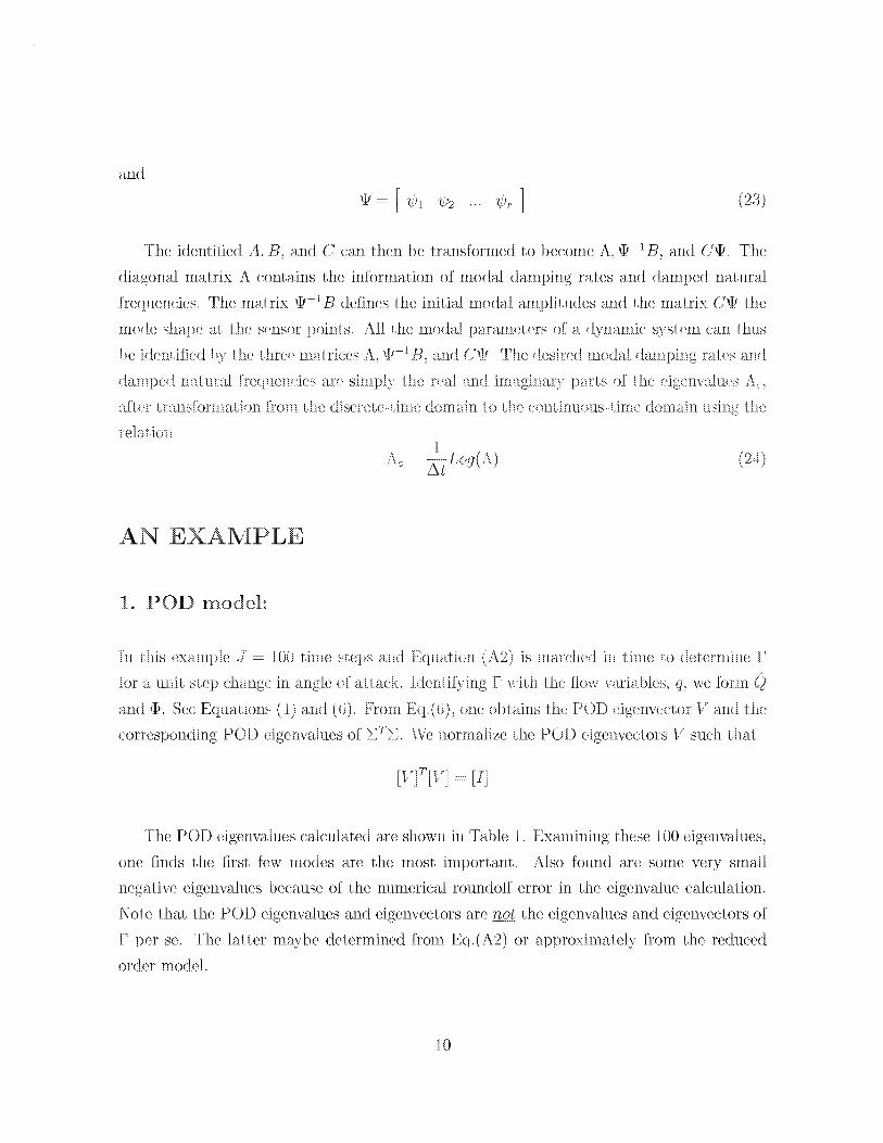
AERODYNAMIC MODEL

The flow about a cantilevered halt-span delta wing is assumed t.o be incompressible, inviscid

and irrotationa]. Here an unsteady vortex lattice method is used to model this flow. |<hn [4]

has also used a similar flow model in his study of the POD or Narhunen-Loevc method lbr a

wing of rectangular p]anform. A typical planar vortex lattice mesh for the three-dimensional

flow over a deha wing is shown in Figure 1. The plate and wak_ are divided into a number

of elements. In tile wake and on the wing all the elements are of equal size, As_ in the

streamwise direction° For the present calculations, the spanwise element size_ A!/, is chosen

to be equal to A¢. Point vortices are placed on the plate and in the wake at the quarter

chord of the elements. At the three-quarter chord of each plate element a collocation point

is placed for the downwash_ the velocity induced by the discrete vortices is set equal to

tile downwash arising fl'om the step angle of attack of the delta wing. Thus one has the

re]ationship_

where w_ +_ is the downwash at the ith collocation point, at time step t } 1, F j is the strength

of [,he jth vortex. F is normalized by cU and w by U where U is the freestream vdocity, k.; 5

is an aerodynamic kernel function. An aerodymanlic matrix equation to determine 1? can be

expressed as,

[A]{N }[B]{r}'. (A2)

when_ [i] and [B] ar(_ a{_rodynamic coefficient matrices and [T] is a transt%r matrix tbr

deternfining the relationship between [,he global vortex lattice mesh and the local vortex

lattice mesh on the delta wing itsel£ Expressions for/k i_ and T are given in Ref.[1]o

From the fundamental aerodynamic theory, the pressure distribution on the wing can be

obtained at the jth poi_t i_ terms of the vortex strengths. The pressure d.il[ere_ce between

the wing plat,e upper and lower surfacesat _; ;_j_y y/is given by

(A3)

The local tot.al lift at. y yj is obtained by integrating the pressure diffi_rence along the

local chord-line

:,;,:,_:t lq¢,', A 'f __:,yj ) ,icIO

where c:o<:,_: cy//l and I is span length and c is the rook chord. The total lift is obtained

by int.egrating the local t,oi.a] lifg along the span.

f

Lt_l / ,_4:t( ._.. "X-" _._:t ,, .=.L':oc,Z,.V:aY cz__Lb:._.z(9.j)A_I.ol/

j J

where A_ 1/k,,. and k_ is the number of spanwise discrete elements. The t,ot,a] aerodynamic

lift coefficient, C:. is defined by

_t_' L.t+l It_rifT2 g(;L - (:\4)/ 2 V_.' _zm , .

:Iwhere A_,, is t,he t,ot,al wing area. In the present, example, A_, _c_ and A_• iG

The numerical mode] is a simple delta wing ......confi_ura.tion vdth a leading e,--l_:,o..._o..._x_.(.""_e:.pof

45 degrees. We use an aerodynamic vort, ex lattice model with 120 vortex elements on the

delta wing (kin kn 15) and 525 vort.ex element.s in _he wake (kmm 50)° The total number

of vort.ex elements is N 645.

SINGULAR VALUE DECOMPOSITION, PROPER OR-

THOGONAL DECOMPOSITION AND BALANCED

MODES: A GENERIC DISCUSSION

[,et q(j) be the nth flow variable at some spatial point at some time j where 'I_ 1, ...,N

and j 1, ...., d. Now [brm the matrix, (D, as

d(1) .......d(J)

N x .I

¢"(i).......¢"(,])

Again note the total nunJ)er of time steps is Y and the total nunJ)er of flow variables is A<

tk)r a typical CFD calculation, d might be 1000 and Ar might be 10000 or more. Hence Az

is much greater than ./.

Now assume a singular value decomposition of <) i.e.

[©] [U][E][N T (2)

where U is a unitary matrix o[ dimension A: x _!,and _r is also a m_itary matrix of dime_sion

,l x }'_,.Olle ma:y select 'ts and b'pioally _'_,will be less than J. Note thai

,

and E is a diagonal matrix of singular values, i.e.

(Ti

cv2

[v]"'[v] (s)

(4)

One may also compute U if'ore Equation i,"'_ and further one ma_ _ compute (_) from a., \ J / .,

knowledge of U, V and the sb_gular values usb_g Equatim_ (2). Usually it is easier So compute

Now order these singular values such that

Form (F, the correlation matrix for the POD method.

[_']------[©F[©i [V][_]'_[f,'_i'_[Ul[_l[vF [VI[EF[E][VF (6)

Equation (6) implies that V is the eigenvector of the correlation matri× and the corresponding

eigem:alues are the squares of the singular values. From Equation (2), one may compute

(assuming that V is normalized so that the magnitude of each eigenvector is unity)

[©][V] [UI[EI[Vi'_[Vi if/Jill (7)

f} directly from Equation (1). Howeverthe representationof Equation (2) maybe usefulif

onechoosesto decomposeQ such that

[0] [v]% (s)

With this decompositio_ the POD modes are said. to be _'balanced. '_ and these are often put

forth as an optinmm choice for mode selection.

If there is a truncation in the singular values, i.e. one chooses <_ to be less than J

which is much less than N, then Equation (2) may be written in a reduced form. The

corresponding reduced [brm for 0 approaches the original <) if the neglected singular values

or POD eigenvalues are su[ficient]y small compared to those retained.

Denoting V as the eigenvector matrix [or the correlation matrix of d.imensio_ J x ',,<

noting that () is a matrix of A; x J, and d.efi_fing, _., as the new tmknow_s to be determined

which are the n modal amplitudes of the POD modes, then o_e may write the original flow

variables, _/, as

Substit.uting this expression into a generic form of the flow equations of motion, i.e.

{d l}

and pre-mu]tip]yingby the transposeof (_)givesa reduced order mode] in terms of the new

unknowns, a ,where the dimension of the vectorc._is'nx ] with 'izchosen to be ]essthan J.

Pbr simplicity, in Equation (10) only a single scalar input., _, is showm The generalization

to multiple inputs is dea> if Q(q) in Equation (10) is expanded in a Taylor Series about a

steady flow solution (the time linearized model corresponds t.o retaining only linear terms in

q in the Taylor Series), then a particuhrly simple and at.t.ractive ibrm of the reduced order

model is obtained.

There is another interesting case to consider which may arise when experimental data

rather than numerical data from a CFD code are used to construct a reduced order model.

In this case the number of flow variables that are observed or mea.sured_ j\r will be relatively

small and typically/V will be less than J, the total number o{ time steps fbr which data are

obtained. I'brrnally the calculationstill goesthrough, but now the numberof flow variables

modeledis muchsmallerthan [br a CFD code.Ideally theseflow variableswouldbe related

to the amplitudesof thedominantmodesof the flowo

SYSTEM IDENTIFICATION

To confbrm to the usual formalisnl of system identification theory, we consider a discrete

time state space model [4]. Note the vortex lattice flow model naturally appears in this

tbrm. l_or continuous time models, the relationship between discrete and continuous time

representations must be carefiflly considered. ['brmally the procedure is similar, however.

Assume that the flow field can be described, by the discrete-time s/a/e-space model,

where ¢(]c) is a state vector of 'r_x 1 ('r_ order of the system), u.(_:) is an input force vector

of 1" x ] (? number of input), ?q(_) is an output measurement vector of f'm. x ] (m number

of output). The matrices A, B, (/, and D, are the state matrix, input matrix, output matrix,

and direct transmission matrix, respectively.

Let v<(0) 1(.i 1, 2,.. ",,,",and 'u,_(,{:) 0(k: 1,_,'_ .) be su.bst.itu.ted into F..q.(11).,

When the substitution is per[brined tbr each input element '_(0) 1(_; 1, 2, ..... 2/), the

results can be assembled into a pulse response matrix Y with dimension _'_zby v as [b]lows:

K, D,_.] CB, t:2 CAB, ...... ,E (TA _ _B (_2)

The constant matrices in the sequence art known as Markov parameters (See [4]).

Assume that the scalar quantity qi(k) in the matrix (_) in Eq.(l) is the pulse response of

the Rh flow variable at the time step k corresponding to a pulse input. A colunm vector Y

can be formed by

(s-,(1)

(s2(1)

(s,,(l)

_,)<2 CA B

?,(2)

_u(2)

.,7,._(2)

, .... _: (17A_ :lB

cs:l(i:)

q2(,_:)+

System idel:ltJficatJon begins by [ormino; the generalized Hankd matrix H(0)_ composed

of t,he Mm'kov parameters

H(0)

This matrix is ident, ioal t.o the mat, l:ix () in Eq.(]) with the absence of the last column. He_:'e

as assumptioz_ has been made; i.e., 'm, > l > 'n. _br the other cases where the munber of

measurement sensors is sul]icient]y less than the order of the sysOem, i.e.; l > 'n, > 'm,; a

diflL'rent Hm_kel matrix can be fbrmed (br s.ystem ident, ificat, ion (see Chapt, er 5 in [4]). The

fundamenca] ru]e is that Che Hanke] matrix musc be R)rmed such Chgt its rank is ]after 1,ha,_

_he order of the s.ystem to be identified.

in t,heorv, the tlankel mat, fix _.,. Ht0_ and the state-space model are related by

H(o)

CB CAB

C[ B AB

t'7, 1]

.... CA _ 2I__]

(15)

'Ib determine A_ B, (7 first decompose the matrix H (0) by using sb_gulam value decomposition

t,o yield

H(0). U)3V"" [U:,. U t] [ 0,__ ,, O'" " ] [I'? Vt]T}',.,_:

..;.,,-,,-TUi:_tvif{-J f L l' li ,f t

r,,..:,,,'._[_i.<.]Lm"7 _ T j

.;omparJson of t_q_.(] o) al:_d (i6) est, ablished the followin_ equalities

(16)

T 'q

_;./'21r A _ 2

The cqua]i ties are not unique_ but t}w.y are ba]a_ced because both share t}w matrix )] equally.

The matrix B is then determined by

L_ The first column of [E_!./2V_.] (18)

rib determine the state matri× A; another Hankel matrix must be tbrmed, i.e°,

This matrix is formed by deleting the first column of H(O) and adding a new column at the

end of the matrix° "\s a result° _, fi t l] has the tbl]owin_ relationship with the system matrices

,4, B_ and (/

[ _",_ _ .... _-i ]

c A B .......A B

(/A [ B AB ....A _ 2B ]

SubstittLtin_ E',q.(17) into Eq.(2(}) thus yields

(20)

The symbol.... ¢ means pseudo-inverse.. The orthonorma] property of U and V showl:_ in Eq.' t_'_oj

has been used to derive Eq(2])

Assume that. the state matrix A of order < has a comp]ete set of ]inear]y independent

eigenvectors t,(h :. 'd'2, ..... :.'d', with corresponding eigenvalues I , .A2,. .... :. l,. which are not. nec-

essarily distinct. Define % as the diagonal matrix of eigel:lvalues and qJ as the matrix of

A

ei_envectors, i.e.,

,'< < • 22)

and

The identified A, B, and C can then be transfbrrned to become A, • _B, and Cq. r. The

diagonal matrix A contains the in[ormation of modal damping rates and damped natural

[requencies. The matrix qJ _B defines the initial modal amplitudes and the matrix (/_[, the

mode shape at the sensor points. All /,he modal parameters of a @namic system can thus

be identified by the three matrices A, • I/_, and (/_[,. Tile desired modal damping rates and

damped natural [requencies are simply the real and. hnaginary parts of the eigem,,ah.l.es A:,

after transJbrmation from the discrete-time domain to the continuous-time domain using the

rehtion

A,, _ I.,,_X.,'X) (2,0

AN EXAMPLE

1. POD model:

In t,his example 3 100 t.ime steps and Equation (A2) is marched in time t.o determine F

for a unit step change in angle of attack. IdentifN,ing [-' with the flow variables, g, we {brm ()

and _. See EquaUons (1) and (6). t_¥om Eq.(6), one obt.ains the POD eigenvector V and the

corresponding POD eigeuvalues of ETE. We normalize the POD eigenvectors V such that

] [i]

Tile POD eigenvalues calculated are shown in Table 1. Examining these 100 eigenvalues,

one finds the fh"st ti-w modes are the most important. Also found are some very small

negative eigenvalues because of the mm_erical roundoff error in t,he eigenvahte calculat, ion.

Note that t,he POD eigenvalues and eigenvect, ors are ','so/t,he eigenvalues and eigenvect.ors of

F per se. The latter mwbe deternfined from Eq.(A2) or approximately from the reduced

order model.

]0

From Eq°(2), we can determine the unitary matrix [,"_

[U] [0][V][Z] _

with a normalization such that [U]'r[U] [1]° i¥om Eq.(A2), we have

{l:}_÷_'+[A] _[B]{F}_ [A] _[T]{,_,}_÷_

I_rom E__t.vig"_j,We have

(2_)

(26)

{_'} [©],,,,x.:[v].,_,,{_},,

Substituting Eq.(25) into Eq.(9), we have

{r} [u][>:]{_.,.} ,_.,j'"_'

Substituting Eq.(27) into Eq°(26), we have

[u][_]{,_}'+:'t[_4] '[L_][U][_]{,_}" [A] _[_"]{_,.,}" (2S)

Pre-multip]yiug by the trauspose of [U][E] gives a reduced order model iu terms of the uew

unki_o_,vns,{_0.

([u][_])"[u][s]{,_,}'÷' +([u][s])"'[_A] '[Bi[u][_]{_0" ([U][_])T[A]_['T]{_,'_,}'*:' (29)

by

\',/]i] eli'e

aD d

Thus a new three-dimensional time domain vortex lattice aerodynamic equation is given

. _ i ._'[t ] toO)

(Y, _ E) I(U E) _ 4 B U "_It1 [:]"_[_] [ I[_ ]_'[_] '[ ][-;]b]

Cenerally, ?_<< N_ and thus a reduced order time domain equation is obtained, ibr the

present example. N 645 and _. < '_(). Once {__} is d_.U.rmm_A from Eq°(30), the {F} _ and

{I"} _ _ can be determined from Equation (26) and _he total lift. coefficiem of the delta wing

is calculated usin_ Eq.(A4).

]]

Figure 2 showsthe tot.a]lift, coefficientof the delta wingvs nondimensiona]time, <, as

determinedfrom thefll]l vort,ex]at.t.ieemodeli.e , usingEq.(A2)with N 645°

Figure S shows the total lift coef[]cieut of the delta, wing vs nondimensiona] time, r, as

determined from the reduced order model for various sizes of the reduced order mode], i.e.

'I_ ], 5 and _. 20, using Eq.(30).

The reduced order model results are very close to the result using the fil.]l vortex lattice

model [or the steady state, r ----+co even fbr 't_ 1. These results are consistent with those of

Table 1_ As seen from t.his table, the POD eigenvalue of the first mode is signiflcant, ly larger

t,han the others. So there is a single dominant, mode and all others have a relatively small

cont, ribut, ion t,o the t,ota] lift. coefficient° However more POD modes are required t,o capture

t,he dynamics of the flow model for shorter times, say 7- < 1, as shown in [_"igure 3_

The aerodynamic eigenvalues of tile vortex lattice model may be determined fi_om Eq.(26)

and an approximation to these eigenvalues may be determined if'ore Eq.(30) by setting the

right h_md sides to zero and determining the condition for non-trivial] solutions in tile usual

way. Results []'om these calculations will be compared to those obtained fiom the system

identification method in tile following discussion.

2. System identification:

Using the time history [br the vort, ex strengths of tile vortex lattice modal at, each grid point,

the system identification procedure described earlier was used to construct a dynamical model

of this system. By using all the in[ormation of tile original modal we can be sure Chat we will

reproduce these same time histories Co some specified accuracy and Chat is indeed, the case.

Within plotting error, the results for t,het, irne hist, ory of tile original vort, ex ]att, ice model

and tha_ of the ident, ified model are identical.

More interesting is t.he number of states required in the system identification model to

achieve this accuracy and how well the eigenvalues of t.he identified model agree wit.h those

of the original model. It turns out that the mmfl)er of states in the identified model is about

,10, i.e. of the same order as the number of stat, es required in t,he POE) model to reproduce

12

the essentialdynamicsof the originalvortex lattice model.

It hasbeenshownin previouswork that the dominanteigenvaluesof the vortex lattice

modelmay be representedby the POD modes.In Figure4 we show a comparison between

tile eigenvalues determined from the fh]l vortex model and those determined from the system

identification model. As is seen the agreement between the two results is excellent for the

corresponding eigenvalues. The identified model in fact has represented the eigenmodes ill

the dominant branch of tile eigenva]ue distribution of the original vortex lattice model and

done so with a high degree of accuracy.

The dominant branch of the eigenvalue distribution corresponds t.o the eigenmodes with

a spanwise pressure distribution similar to that tbr the life on a wing at steady angle of

attack. Other branches of the eigenvalue distribution correspond to higher spanwise modal

fornlso

A system identification (SID) model fbr an unsteady aerodynamic flow has been created

fbr several wing motions or gust excitations and corresponding aerodynamic responses. These

models were derived fi'om numerical simulations using a vortex lattice (VL) mode] for the

delta wing with 55 vortex elements on the wing and 300 vortex elements in the wake (e.g.

km kn 10, kmm 40 as shown in Fig. 1). Ill each case, the flow about the wing is excited

by a certain type of prescribed downwash at the wing grid points, tu(t). The numerical VL

model produced vortex strengths at the grid points of tile wing and in tile wake, F(t), and

the corresponding pressure distribution on the wing, l)(t). These data were then used as

input for the SID code.

Tile excRadons to the ftow that have been considered are

1) step angle of attack, _,(t) cor_t for t > O,

2) sha } c dgegust, ..... rot ...... > o,

3) frozen gust of changing tYequency,

such a gust is sometimes called a swept gust, and finally

13

4) random downwash ('_u at each grid point and at. evory time step is a random mmlber).

First, the SID mode] was used to reproduce the tirue histories of the vortex strength

(on the wing and in the wake) [or 100 time steps. Results obtained [rom tile SID model

were almost identical to those of tile original VL model. Tile plots of such time histories are

not provided here, because one would not be able to see the diffbrence in the time series of

the original data and the time series obtained via SID+ However, to quantif); the differences

between VL and SID outputs a.n error, 5_ def]ned as 8 ]00%[({? - .VI/[(_)[ was used, where

the norm [-<YI]s defined to be the largest sin_;u]ar value of X. In this case, both (_? (VL) and

7/(SID) are ]00 x 35,5 rectangular matrices (]00 time steps and 3,5,5degrees of freedom). Eor

1,he above menl, ioned aerodynamic problems, a_d givon the vorl, ex sl,rengths evorywhere, the

error was less than 0.05%. Moreover, using; the VL time series fbr the vortex strengths only

on the wing, the SID model reproduced them with alruost the same accurac), the largest

(among the aforementioned cases) error was 0+] _,_[:.The nmnber of singular values retained in

1,he identified model varied [7om 60 1,o !)0 tbr/he cases when vor/,ex s/re_gths were provided

onl), on the wing and from 60 to 160 for the cases when the SID used vortex strengths both

on 1,he wing and in the wako. (The number of singub, r values kept, w_,s such that 1,he ratio

of the lar_;est singular value to the smallest one kept was _0 -,2)

Next, t,he ability of such a SID model to capture 1,he eigenmodes of 1,he original VL system

and especiall), the dominant eigenmodes was st.udied. Here again, all t,he infbnnal,ion on the

wing and wako was used initially, and t,hen the infbnnat.ion only on 1,he wing was used to

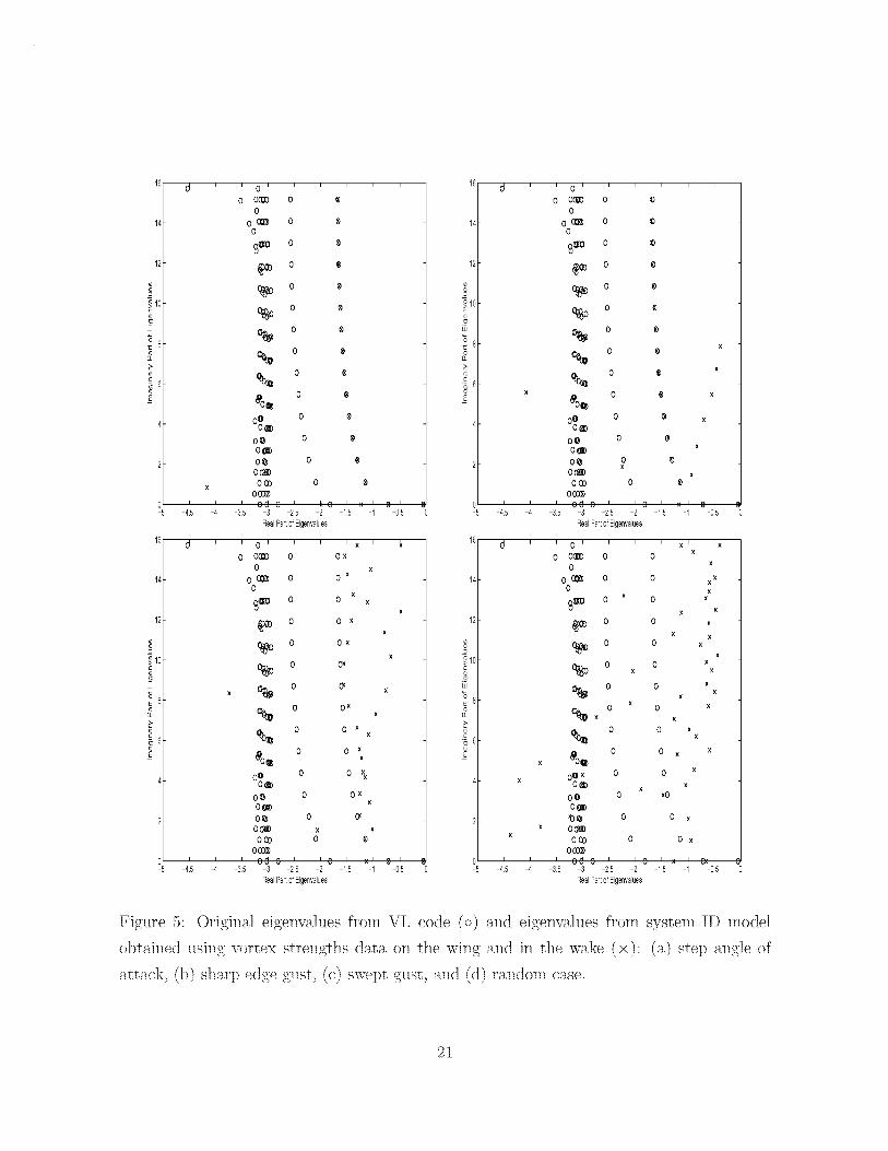
obt.ain the eigenvalues. The fbrn_er case is shown in t'_igures [J and 6 and t,he latter in ["igure 7°

Here the original VL eigenvalues are shown as circles and 1,he eigenvalues obtained ifore the

SID model are indical, ed by crosses_ In 1,he case of fifll information_ the dominam eigenvalue

branch for t.he case of a st,ep angle of attack (Wig. [Ja) and also a sharp edge gust (_'_ig. 5b)

is captured nicely (36 singular values and 5Y singular values were used respect.ivoly in the

SID model), bbr t.he case of a swept, gust (["ig. 5c) and random downwash (_ig. [Jd), the

SID model produced set.s of eigenvalues t,hat do no_, agree well with t,he original ones fTom

1,he VL code (164 singular values and 99 singular values were used respectivoly in the SID

model). Howevor, fbr t,he problem of 1,he random downwash, increasing the length of the

1,ime him, ory that was used as input, t.o the SID model code from 100 steps to 1000 st,eps lead

t,o a set of eigenvalues that, is in vory good agreement wil, h the dominant branch as shown

]4

in Wigure 6 (%0 singular values were used).

When tile vortex strengths only on the wing were used fbr sorue initial selection of

parameters in the SID model (see FIg. 7): interestingly the dominant branch of eigenvalues

is recovered not only for the step angle of attack (Fig. 7a) and the sharp edge gust (Fig.

7b): but also for the case of the swept gust (Fig. Tc) and random downwash (Fig. Td),

even though ]n the last case the dominant branch ide_ttifled by the SID mode] is somewhat

_'off target '_. By looking at the Figure 7 one ru]ght conclude that providing vortex strength

infbrmation only on the wing in these cases is sufficien¢ for finding the distinct domimmr

eigenvalue branch. However: one should not conclude that using vortex strength in[ormation

on t,he wing only is ac6ually bet, t,ert, han using intbrmation about vort, ex strengths both on

the wing and in the wake.

By running t,he SID code tor various parameter choices and [or a cert, ain number of

retained singular values_ diffbren_ lengl, hs of t,ime series_ using in[bnnal, ion on _he wing only

vs intbrmat,ion everywhere, et,c_ the authors have found, flrsl, ly, t,hat the se_ of eigenvalues

iT"ore t,he SID model could either include 1,he _'correc_ '_ dominant eigenvalue branch or could

be a diflbrent set of eignvalues (which_ by _he wa_.', does nol, prevent, _he SID model iTore

reproducing the original time series wit, h excelle_t _,greeme_t); secondl3.'-, i¢ was concluded

1,hat if there is a distinct, branch of eigenvalues tbund iT"ore the SID model, it, is mosl, likely

t,o be similar to t,he dominant branch in 1,he original VL model.

Now another case will be considered. In the co_ttext of wing tunnel or flight experiments:

one is also interested in what can be identified fi'om the measured data such as pressure.

So using mxruerica]]y obtained pressure values over the wing, the SID model was used to

reproduce pressure time histories. Just as in the case of vortex strength data on the wing

only_ ,55 pressure time histories of _00 time steps were input to the SID code. Using 30 to

40 singular values, the error between the original and identified time histories of pressure

remained less than ]%.

One could argue that it, may be impract, ica] t,o use such a large amount of sensors on the

wing to apply SID models. Thus, next only a portion of 1,he pressure data on t,he wing was

used. Diffbrent, sensor positions wore considered. A discussion of t,he various downwash and

sensor local, ions on such a wing is ommit, t,ed here. For 1,he currem discussiom leading edge

15

elenlents from the root. to the tip of the wing were taken, as t.hey appear to be a very good

choice for system identification purposes. In Figure 8, results tbr the pressure time history at

the tip elemem of the wing are shown for the case when 10 measurements (still numerically

simulat, ed, of course) of the downwash and pressure dine history (100 time steps) along the

leading edge were supplied t.o create the SID model. Using from 50 to 90 singular values for

t,he four aerodynamic loading problems, t,he previously defined error ranged 9ore 0.002% to

.8%.

However, using pressure data only, no success has yet been realized in approximating the

eigenva]ues of the original VL model. This is a subject of continuing investigation.

CONCLUDING REMARKS

it. has been shown that a modal representation of the aerodynamic fbrces acting on an

oscillating wing has several attractive f(_a/ures /hat n_y be exploited. As has been shown

earlier, st.art.ing from a numerical model of the fluid, here tahm t.o be a vort, ex lattice model,

the fluid model may be efficiem]y represented, in/,erms of Proper Orthogo_a] Decomposition

(POE)) modes° ][tow<_ver it was also shown that, using st,andard system idemiflcadon t.ech-

niques tbr linear dynamical systems, an idemJfied system model may also be constructed

using data Kern the numerical model. Bot, h the POD modes and the syst, em identification

me/hod lead t,o substamJally reduced order models of the flow field of comparable dime_-

sions. And therefore both provide highly efficient computational models relat.iv{_ to the

original vortex lattice] numerical model.

In principle the POD method may also be used %r nonlinear dynamical systems. [_ow-

ever much work has yet to be done to implement this capability in the context of unsteady

aerodynamic models. The system identification ruethodo]ogy for nonlinear dynamical sys-

tems is still a research ff'ontier and no general methods are yet available. On the other hand

the systems identification approadl may be useful when only partial flow field data are avail-

able, e.g. from a wind tunnel experiment, and this aspect is currently under investigation

by the authors.

Finally it is noted that although a particular numerical model of the fluid was used i_ the

]6

present,paper,i.e. a vortex]at.ricemodel,noespecialdifficulty is expectedin extendingthese

met,hodsto other Comput.at.iom_lFluid Dynamics(CFD) models°indeedthe beneficialuse

of PODfor a varietyof CFDmodelshasbeenshownin [1-3].Sincethesystemidentification

modelonly requirestime historiesor Fourier Series(frequencydomain)dat.afk'omsuchaCFD model, the extensiont.oany t,imelinearizedCFD model is st,raight.tbrward.Indeed

evenif the original CFL)model is not,time ]inearizedper se,the codecanbe run for snm]l

wing motionsto simulat,e mmlerically dine ]inearized conditions°

ACKNO_,VLEDGMENTS

This work was supported under AFOSR Grant, "Limit Cycle Oscillations and Nonlinear

Aeroelastic Wing Response". Dr. Daniel Sega]man is the grant program officer. All numeri-

cal calculations were done on a supercompuBer; Tg](i, in t,he North Carolff]a Supercomputing

Cemer (NCSC).

REFERENCES

1. Hall, K.C., " Eige_mnalysis of Unsteady F'lows About Airfoils, Cascades, and Wings;"

AL'IA ,Io'_,rr_ai, Vol.32, No.12, 1994, pp. 2426-2432.

. Dowell, E.t£, Hall, K.C., and Romanowski, M.C., " Eigenmode Analysis in Unsteady

Aerodynamics: Reduced Order Models," .,lpplied /Mec/,.,ar,,'ics Rev_et,';.< Vol.50, No.6,

June ] 997, pp. o ¢1-3,8o.

3. Dowell, E.t£ and Hall, N.C., _' Modeling of Fluid-Structure Interaction," Invited Chap-

ter in the A_'r,,,_,al f{e'_;{eu,s of FI._i4 mecl',,o,r,ic< Vol. 3_< 200], pp. 445-490.

4. Kim, T., _'PYequency-Domain Karhunen-Loeve Method and Its Application t.o Linear

Dynamic System," 414A Jo'u,,,'_m.l, Vo]. 36, No.ll, November 1999, pp.2117-2123.

5. Juang, J.-N., Applied S:qstc'm ]dentificat'ion, Prentice Hall, Inc., Englewood Cliffs, New

J<]_.{,.,_'< _v (}7632, i994, [SBN. 0-1,-)-0'_¢c},).... 1]-X._

17

Iable ]: Eigenvalues; q,

c_1 2_ cv2_ s0 ,7sl 7s CrT,,._iooi

0.31168E" 03 0.a16odF_ t O0 [ 0.82697F..-05 -0.33688E-05

0.33737E+02 0 50.582E+00. -t._.04a0E-0o, -0.30680E-05

0.3918dF].l 0] 0.d90oOE} 00 -u._ _{_]]E-0a -0.200,8E-0oT

0.31482Ei 0l 0.d8854E I00 -0.72553E-05 -0.27129E-05

0.25025E'01 0.48179El 00 i 0._ooaOE.-0a -0.22659E-05

0.20812E+0] 0.47621E+00 ! 0.72555E-05 , -0.16534E-05

0.17607El 0] 0.4/1,1E, 4 00 -0.69035E-05 0.32531E-ua

" _ 0.29655E-050.15281El 01 0.d6827E t 00 -0.65890E-0a ..

0.]3464E'01 0.4658dEt O0 i -0.62088E-05 0.28340E-05[ •

0.1205lEf 0l 0,46439El O0 i -0.64251E-05 0.25623E-05

0.10909Ei 0] 0.]a028E4 00 -U.o_]dlE,-0a 0.24380E-05

0,99799Ei 00 0._o_IE-02 0.65583E-05 -0.13306E-05

0.92088E+00 t.._.4(.4_E-04 [ 0.64960E-05 -0.]]599E-05[ •

0.85612Ef00 -0.17071E-0d [ 0.60496E-05 -0.84823E-05

0.80130E+00 0.13413E-04 0.57069E-05 -0.46961E-05........................................................................................................ t ......................................................................................................

0.75427Ei 00 0.12234E-0d -0.52226E-05 -0.3d102E-06

" }' ,R ...... ' ' _ }"0.71385E+00 -0.]0651E-(4[-0.4_-20]E-0a -0.122b0E-(Vr •

0.678(i7EfO0 -0.I0369E-O'I[ -0.42629E-05 0.18361E-05

• ) _] 4 I "]0.64_]aEm0t 0.1]27]E-04 0.49989E-05 0.17704E-05........................................................................................................t......................................................................................................

0.62129E i 0(} 0.]0661E-(}d 0.:l, , _Sg-0,.. 0 ]4_15E-(}5

] -o , <;_ :0.59783E+00 -0.90705E-05 [ 0.4738]E-05 t..l_]4tE-0o........................................................................................................ [....................................................................................................

_vv ,__' _ 0 90622E-050.o I_E, 00 .... [ 0..I3455E-05 0.10583E-05

0.55896E+00 0.96568E-05 0.,99.9, E-0__ 0.4438]E-06........................................................................................................ t ......................................................................................................

0.54293Ei 00 0.90_64E-ua -{L37350E-05 0.49844E-u0

0.,52889E+00 -0.85099E-05i-0.35918E-05 0.60061E-06

18

air flow

Figure 1: Numerical grid %r delta wing-plate using vortex lattice aerodynamic ]-node]

¢)

000

5o

11

10

9

8

7

6

5

4

3

2

10

I I I I I I

I I I I I I

1 2 3 4 5 6 7

nondimensional time

Figure 2: The total liR coefficient of the delta wing vs nondirnensiona] t,ime, T, %r all modes

]9

3.5

3©eO

•- 25

22

1.5

I I I I I I

'n=all''n=l' - .......,n=5 ..........

'n=20' o

0 1 2 3 4 5 6 7

nondimensional time

Figure _'' ",-o. The t.ot.al lift, coetlident, of t,he delta wing vs nondimensional t.ime, ,, [br r_, 1,5

and 'n 20

.,=

0

-10

-20

-30

-40

-50

-60

-70

-80

-90

-100

I I I I I

®®®®®®® O • O_ilI

® • • -ires, iNkY _

o,l'J

°'1

d_._.._am,._ I I I I_ww w

0 2 4 6 8

Frequency,Hz

Figure 4: Eigenvahie so]ut, ions oI vort, ex lat, t,ice model of unst, eady tM :._-d.]]mm_lona] flow

about, a delta wing. Eigenva] ues dot,ermined direct, ly from the vorl, ex lat, t,ice model: o Dom-

es?; .... _,_, All or,her eigenvahies; Eigenvalues from system i&,ntificationinant, branch of (,l_cn\,alu_. • . .,

model: x.

20

12

LJ

_8

b

E

i i O i i i i i

0 0(]00 0 g

0

00_ 0 ®0

8_ o

% o ®

_0_ 0 ®

00@ 0 ®

O_ 0 ®O_O@ 0 ®

000 0 ®

OOU_

12

LU

_8

c

) 6E

0 ' ' ' 8d C ' _ O ' :: ' @ '-5 -45 -4 -35 -3 -25 -2 -15 -1 -05

RealPartof Eigenvalues

16 d ' ' o' ' ' 'x ' k0 O(gO 0 0 x

0 x14 00_ 0 0 x

0X

Q_ o o xu

×

0 0 xv_

X

(_ 0 Ox×

I:_ 0 _ xX

_1_ 0 0 x x

0 0 x x

0 0 x_o_ x

4 Oo0 0 0 xx

00 0 0 xO_ x

2 O@ 0O@]m) x x

OCO 0 gOlIg)

O ' ' ' C_ C ' ' O ' ::' _ '-5 -45 -4 -35 -3 -25 -2 -15 -1 -05

RealPartof Eigenvalues

710_gLJ

=8

b

E

12

W

_8

_c_6E

i i 0 i i i i i i

0 O_ 00

OO_ OO

8_ o

X

O g x

x 0 ® x

O0 0 @ xO_

O@ 0O_ x

O@ 0 _gx

O_lg xOCO 0 g

O_0 i i i odo i i o i _ i ® i ,-5 -45 -4 -35 -3 -25 -2 -15 -1 -05

RealPartof Eigenvalues

16 d ' ' 0 ' ' ' ' x' 'x

0 OQ]O 0 0 x0 x

14 0 _ 0 0 x x0 xo_I_ 0 x 0 x

x x

_0 0 0 x,r#

X×

0 0 xX

O_ 0 × 0 ×x

0 0 x xx0 x 0 x

_× x0 0 x%

_0 0 0 x xx

o_X 0 0 x4 X

O_X X

0 @ 0 xOO_

2 _0@ 0 0 xx 0(_

XOCO 0 0 x

0(_

0 ' ' ' oO o ' 'o ' ;(' _(' ,-5 -45 -4 -35 -3 -25 -2 -15 -1 -05

RealPartof Eigenvalues

Figure 5: Origina,] eigenvalues from VL code (o) a_nd eigenva]ues from system ID model

obta,i_ed usi_g vortex strengths da,ta_ on the \vi_g _ud in the wake (/): (a,) step a,_z_gleof.

attack, (b) sharp edge gust; (c) swept gust, _¢ud (d) random case.

2]

16

14

12

c0

_1oE_JO)

L.U

_8

0_

c

E

d I

0 I I _

-5 -4,5 -4

t xO ix _ i i t i

0 O(lO0 x_xx ®

o x _00_ _xx ®

o _xn_l_ x (_xx ®

x_x ®

q_ x_xx ®_xx

X_x ®X X

O_D x _xx ®X XX X

X

%X xxX

_ ®

_o_x x_x_ ®O0 x x._X ®

O_ x x ®O_

o_ Xxx_C_ ®

o_ _OCO x x_ O_ ®

000_i 0d 0 _l _,, i _ i i _ i

-3,5 -3 -2,5 -2 -1,5 -1 -0,5

RealPartofEigenvalues

Fig_lre 6: O_:'i_i]:_aJ eigel:walues item V[,, code (o) a,nd eigenva,hles h:'om system ID model

obt, ai_ed ush_g vorl_ex sn:e_gths d.at, a o_ t,he wing ._¢nd in [,he wa,ke (x) re1: l_}_e ra_ndom cause

when time sezJes lengt, h is incze_msed 10 _,imes t,o 1000 dine steps.

22

12

2

LU

b

E

d

x

x

X

X

12

U

_8

>,

c

) 6E

i x i 0 i i i i i

x 0 0(]00 0 ®

0

OQ_ 0 ®0

8_m o ®

_0_ 0 ®

0_ 0 ®

O_ 0 gO_O@ 0 ®

000 0 ®

OOCGD

0 I I I O0 0 I I Ox I I ® I

-5 -45 -4 -35 -3 -25 -2 -15 -1 -05

RealPartof Eigenvalues

16 d ' _ o ' ' ' ' x' '0 OODO 0 @

x 0 x×

14 0 (_ O @x 0

8_ o×

_0 0 (_x

oX

0_ 0 (_x

0 (_X

X

X

0X

X

oo o _4 x 0 _}

O@ xO @

2 O@ 0 @

OCO 0 @x OOC_

0 ' :: ' ' O _ C ' ' O 'x ' _ '-5 -45 -4 -35 -3 -25 -2 -15 -1 -05

RealPartof Eigenvalues

2

U

o ,

_8

E

d

X

X

X

xl X I 0 i i i i i i

0 OQSO 0 @

0

O0_ 0O

8_ o

ol_ o •

_0_ 0 @

OO 0 @O_

O@ 0 @

O_

O@ 0 @

O_

OCO 0 @

O_

0 i i i Od O i i 0 )_ i g i i-5 -45 -4 -35 -3 -25 -2 -15 -1 -05

RealPartof Eigenvalues

16 d× ' xx' 0 '

0 OQIO 0x 0

14 0 _1_ 0x 0

x 8_ o

12 x _ 0

x

°m 0

_8

>,

_ o

_E @Om o

4 08 OO_

O@O_

2 O@O(_

XOCO

Og]@

-5 -45 -35

I I I I I

x O

x O

x O

x O

x O

x O

x O

x O

x O

x O

O

O

O

'C-4 -3 -25 -2

RealPartof Eigenvalues

x O

xO

xO

@

-15 -1 -05

Figm:'e 7: Origina,l eigenvalues from VL code (o) a_nd eigenvalues from system ID model

obtaJned using vorte× sti:'engths data on the wing only (x) _ (a,) step a,ngle of attack, (b)

sharp edge gust, (c) swept gust, a_ud (d) random case.

23

0031

¢

002c¢

o.

E

0027

z

002C

00240 2 4 6 8 10 12

Nondimesional time

-00_

0 2 4 6 8 10 12 14 16 18 20

Nondimesional time

0035

003

0025

¢

002

E 0015

001

0005

d,2

002

O0

o.

ool

O0

000

i i 1'01'2 1'41'6 1'820NondimesionalUme

®

i i i i i i i i i

2 4 6 8 10 12 14 16 18 20

NondimesionalUme

Figm'e 8: Time series of the pi'essm'e at the tip element. Original VL code data (solid line

with o's) and resulted time series from system ID model obtained using pI-essm-e on only 10

leading edge element.s as input (dotted line wit.h x%): (a) step angle of attack, (b) sharp

edge gust, (c) swept gust, and (d) Iandom case.

24

REPORT DOCUMENTATION PAGE Form ApprovedOMB No. 0704-0188

Public reporting burden for this collection of information is estimated to average 1 hour per response, including the time for reviewing instructions, searching existing datasources, gathering end maintaining the data needed, end completing end reviewing the collection of information. Send comments regarding this burden estimate or eny otheraspect of this collection of information, including suggestions for reducing this burden, to Washington Headquarters Services, Directorate for Information Operations endReports, 1215Jefferson Devis Highwey, Suite 1204, A#ington, VA 22202-4302, end to the Office of Menegement end Budget, Peperwork Reduction Project (0704-O188),Weshin_Iton, DC 20503.1. AGENCY USE ONLY (Leave b/an/0 2. REPORT DATE 3. REPORT TYPE AND DATES COVERED

December 2001 Technical Memorandum

4. TITLE AND SUBTITLE 5. FUNDING NUMBERS

System Identification and Pod Method Applied to Unsteady Aerodynamics

6. AUTHOR(S)

Deman Tang, Denis Kholodar, Jer-Nan Juang, and Earl H. Dowell

7. PERFORMING ORGANIZATION NAME(S) AND ADDRESS(ES)

NASA Langley Research Center

Hampton, VA 23681-2199

9. SPONSORING/MONITORING AGENCY NAME(S) AND ADDRESS(ES)

National Aeronautics and Space Administration

Washington, DC 20546-0001

WU 706-32-21-01

8. PERFORMING ORGANIZATIONREPORT NUMBER

L-18119

10. SPONSORING/MONITORINGAGENCY REPORT NUMBER

NASA/TM-2001-211243

11. SUPPLEMENTARY NOTES

Tang, Kholodar, and Dowell: Duke University, Durham, NC; Juang: NASA Langley Research Center,

Hampton, VA.

12a. DISTRIBUTION/AVAILABILITY STATEMENT

Unclassified-Unlimited

Subject Category 05 Distribution: Nonstandard

Availability: NASA CASI (301) 621-0390

12b. DISTRIBUTION CODE

13. ABSTRACT (Max/mum 200 words)

The representation of unsteady aerodynamic flow fields in terms of global aerodynamic modes has proven to be

a useful method for reducing the size of the aerodynamic model over those representations that use local

variables at discrete grid points in the flow field. Eigenmodes and Proper Orthogonal Decomposition (POD)

modes have been used for this purpose with good effect. This suggests that system identification models may

also be used to represent the aerodynamic flow field. Implicit in the use of a systems identification technique is

the notion that a relative small state space model can be useful in describing a dynamical system. The POD

model is first used to show that indeed a reduced order model can be obtained from a much larger numerical

aerodynamical model (the vortex lattice method is used for illustrative purposes) and the results from the POD

and the system identification methods are then compared. For the example considered, the two methods are

shown to give comparable results in terms of accuracy and reduced model size. The advantages and limitations

of each approach are briefly discussed. Both appear promising and complementary in their characteristics.

14. SUBJECT TERMS

System Identification, Unsteady Aerodynamics, Proper Orthogonal Decomposition,

State-Space Model Reduction.

17. SECURITY CLASSIFICATION 18. SECURITY CLASSIFICATION 19. SECURITY CLASSIFICATIONOF REPORT OF THIS PAGE OF ABSTRACT

Unclassified Unclassified Unclassified

NSN 7540-01-280-5500

15. NUMBER OF PAGES

2916. PRICE CODE

A0320. LIMITATION

OF ABSTRACT

UL

Standard Form 298 (Rev. 2-89)Prescribed by ANSI Std. Z-39-18298-102