System Dynamics II

Core module in Fall Semester

Dr. Albert Tan

1

The Manufacturing Supply Chain

• This chapter adapts the stock management structure of the previous chapter to represent the supply chain in manufacturing firms

The stock management structure…

• Is broken up into– An order fulfillment structure– A production starts structure– A demand forecasting component

• Download the Vensim models at – http://www.mhhe.com/business/opsci/sterman/

models.mhtml– Chapter 18 -

Stock S

Adjustment forStock AS

Desired Stock S*

Stock AdjustmentTime SAT

Loss Rate

Desired AcquisitionRate DAR

Supply Line SLAcquisition Rate

AROrder Rate OR

Acquisition LagAL

Expected LossRate EL

IndicatedOrders IO

Adjustment forSupply Line ASL

Desired SupplyLine SL*

Supply Line Adjustmenttime SLAT

AverageLifetime L

Expected AcquisitionLag EAL

An order fulfillment structure

Policy Structure of Inventory Management

Work in ProcessInventory

InventoryProduction Rate Shipment RateProduction Start

Rate

Customer OrderRate

Order Fulfillment

demandForecasting

ProductionScheduling

B

WIP Control

B

Inventory Control

B

Stockout

Figure 18-1

Three Balancing Loops

• Stockout loop regulates shipments as inventory varies

• Inventory and WIP Control Loops adjust production starts to move the levels of inventory and WIP toward their desired levels

In this initial model there are…

• No capacity constraints (from either labor or capital)

• No stocks of materials

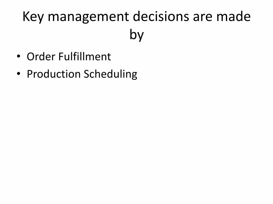
Key management decisions are made by

• Order Fulfillment• Production Scheduling

InventoryShipment Rate

InventoryCoverage

Customer OrderRate

Desired ShipmentRate

Order FulfillmentRatio

MaximumShipment Rate

Table for OrderFulfillment

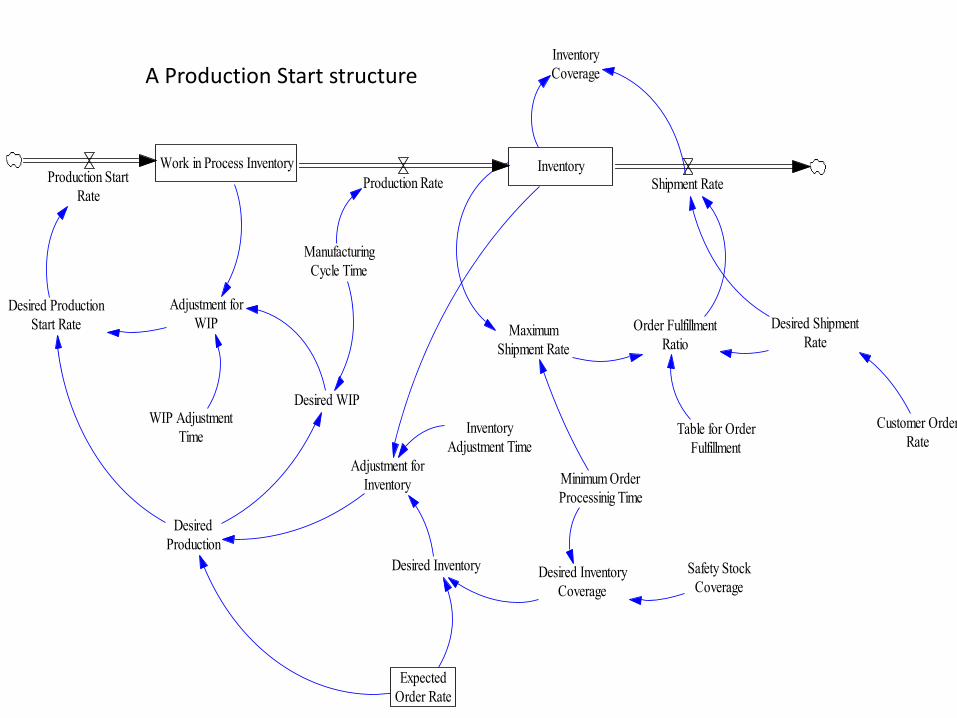
Work in Process InventoryProduction RateProduction Start

Rate

Adjustment forWIP

Desired ProductionStart Rate

ManufacturingCycle Time

Desired WIPWIP Adjustment

Time

DesiredProduction

ExpectedOrder Rate

Desired Inventory Desired InventoryCoverage

Safety StockCoverage

Minimum OrderProcessinig Time

Adjustment forInventory

InventoryAdjustment Time

A Production Start structure

Production Structure

InventoryWork in Process

InventoryProduction StartRate

Production Rate

ManufacturingCycle Time

Production

Production Rate =

• DELAY3(Production Start Rate, Manufacturing Cycle time)

Terms

• Manufacturing Cycle Time—the average transit time for all items aggregated together in the model

• Manufacturing delay is being modeled as a fourth-order material (flow) delay

An Order Fulfillment Structure

InventoryShipment Rate

InventoryCoverage

Customer OrderRate

Desired ShipmentRate

Order FulfillmentRatio

MaximumShipment Rate

Table for OrderFulfillment

Desired InventoryCoverage

Safety StockCoverage

Minimum OrderProcessinig Time

InventoryAdjustment Time

Table for Order Fulfillment

• From Fig. 18-3

Desired Shipment Rate =

• Customer Order Rate

Order Fulfillment Ratio =

• Table for Order Fulfillment(Maximum Shipment Rate/Desired Shipment Rate)

Maximum Shipment Rate =

• Inventory/Minimum Order Processinig Time

Other constants

• Minimum order processing time = 2 wks• Safety Stock Coverage = 2 wks• Manufacturing Cycle Time = 8 wks• Inventory Adjustment Time = 8 wks• WIP Adjustment Time = 2 wks

Adjustment for Inventory =

• Difference between desired inventory and actual inventory, all divided by the Inventory Adjustment Time

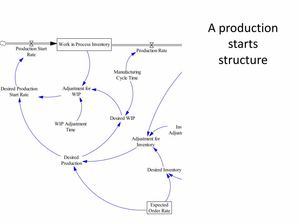
A production starts

structureWork in Process Inventory

Production RateProduction StartRate

Adjustment forWIP

Desired ProductionStart Rate

ManufacturingCycle Time

Desired WIPWIP Adjustment

Time

DesiredProduction

ExpectedOrder Rate

Desired Inventory

Adjustment forInventory

InventoryAdjustment Time

Desired WIP =

• Manufacturing Cycle Time * Desired Production

• This is an implementation of Little’s Law– Inventory =Throughput × Flow Time

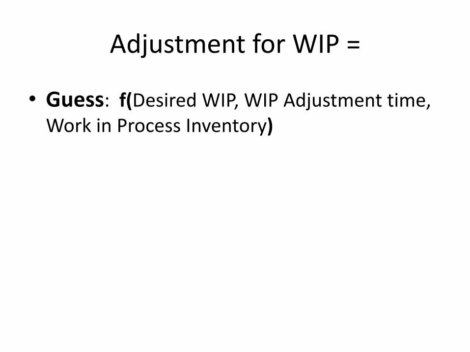
Adjustment for WIP =

• Guess: f(Desired WIP, WIP Adjustment time, Work in Process Inventory)

Desired Production =

• MAX(0, Expected Order Rate + Adjustment for Inventory)

Desired Production Start Rate =

• Adjustment for WIP + Desired Production

Production Start Rate =

• MAX(0, Desired Production Start Rate)

A demand forecasting component

• This structure simply smoothes the customer order rate, much like exponential smoothing would do to provide a realistic model of the forecasting process used in many firms

The demand forecasting structure

Customer OrderRate

ExpectedOrder Rate Change in Exp

Orders

Time to AverageOrder Rate

– What is the equation for Change in Exp Orders?

Typical constants

• Minimum order processing time = 2 wks• Safety Stock Coverage = 2 wks• Manufacturing Cycle Time = 8 wks• Inventory Adjustment Time = 8 wks• WIP Adjustment Time = 2 wks

Initial Stocks for Equilibrium

• Initial Inventory = Desired Inventory• Initial WIP = Desired WIP• Initial Expected Order Rate = Customer Order

Rate

• These are all the initial conditions needed to create an initial equilibrium

Behavior—Inventory

• Inventory drops below desired inventory

Inventory vs. Desired Inventory60,000

50,000

40,000

30,000

20,0000 5 10 15 20 25 30 35 40 45 50

Time (Week)

Inventory : run2Desired Inventory : run2

Behavior—The Rates

The Rates15,000

13,250

11,500

9,750

8,0000 5 10 15 20 25 30 35 40 45 50

Time (Week)

Customer Order Rate : run2Production Rate : run2Shipment Rate : run2Production Start Rate : run2

What the rate Behavior Over Time (BOT) charts tell us?

• Amplification of the customer order rates by the production starts rate is unavoidable– This is what causes the bull whip effect in supply

chains, especially when suppliers are linked to the manufacturer by JIT Kanban or signaling systems

• There is a phase lag between receipt of the order and its fulfillment

• There is no significant oscillation

What about backlogs?

• Boeing, like not other manufacturer, carries backlogs stretching out years.

• Boeing is a make to order manufacturer• Consideration of backlogs modifies the order

fulfillment structure

The backlog

structure

InventoryShipmentRate

B

-

+

DesiredShipmentRate

+

BacklogOrderRate

OrderFulfillment

Rate

+

++

TargetDeliveryDelay

-

B

OrderFulfillment

DeliveryDelay+ -

Backlog equations

• What is the equation for backlog?• The equation for delivery delay is formulated

from one of the most important principles in Operations Management—Little’s Law:– Delivery delay = backlog/order fulfillment rate– Desired Shipment Rate = Backlog/Target Delivery

Delay

More Backlog Equations

• Order fulfillment rate = shipment rate• These are, however, totally different entities• Shipment rate is a physical flow• Order fulfillment rate is an information

accounting that reduces the amount of backlog within the computer’s database

ProductionStart Rate

DesiredProductionStart Rate

B

WIP Control

+

+

+

<ShipmentRate>

-

MaterialsInventoryMaterial

DeliveryRate

MaterialUsage Rate

MaterialUsageRatio

Table forMaterialUsage

MaximumMaterial

Usage Rate

MinimumMaterial

InventoryCoverage

+-

+

+B

MaterialsStockout

DesiredMaterial

Delivery Rate

Adjustmentfor MaterialInventory

DesiredMaterial

Inventory

MaterialSafety Stock

Coverage

+

+

-

+

B

MaterialsControl

MaterialsInventoryCoverage

<MaterialUsageRate>

<MaterialsInventory>

+-

MaterialUsage per

Unit

DesiredMaterial

Usage Rate

+

+

FeasibleProductionStarts fromMaterials

-

++

+

+

+

+

MaterialInventory

AdjustmentTime

- DesiredMaterial

InventoryCoverage

+

+

+

InventoryProduction

RateShipment

Rate

DesiredProduction

Adjustmentfrom Inventory

DesiredInventory

ExpectedOrder Rate

Change inExp Orders

InventoryAdjustment

Time

DesiredInventoryCoverage

Time to AverageOrder Rate

OrderFulfillment

Ratio

Table forOrder

Fulfillment

Work inProcess

InventoryProductionStart Rate

ManufacturingCycle Time

Adjustmentfor WIP

Desired WIP

DesiredProductionStart Rate

WIPAdjustment

Time

B

Stockout

B

Inv entoryControlB

WIP Control

-

-

+

+

+

++

--

+

+

-

-+

+

+

+

+

-

DesiredShipment

Rate

MaximumShipment

Rate

MinimumOrder

ProcessingTime

+

+

-

+ SafetyStock

Coverage

+

BacklogOrderRate

OrderFulfillment

Rate

+

++Target

DeliveryDelay

-

<Customer OrderRate>

+

B

OrderFulfillment

DeliveryDelay+ -

<DesiredShipment

Rate>-

InventoryCoverage

<Inventory>

+

<ShipmentRate>

-

MaterialsInventoryMaterial

DeliveryRate

MaterialUsage Rate

MaterialUsageRatio

Table forMaterialUsage

MaximumMaterial

Usage Rate

MinimumMaterial

InventoryCoverage

+-

+

+B

MaterialsStockout

DesiredMaterial

Delivery Rate

Adjustmentfor MaterialInventory

DesiredMaterial

Inventory

MaterialSafety Stock

Coverage

+

+

-

+

B

MaterialsControl

MaterialsInventoryCoverage

<MaterialUsageRate>

<MaterialsInventory>

+-

MaterialUsage per

Unit

DesiredMaterial

Usage Rate

+

+

FeasibleProductionStarts fromMaterials

-

++

+

+

+

+

MaterialInventory

AdjustmentTime

- DesiredMaterial

InventoryCoverage

+

+

+

Business Dynamics

Business Dynamics

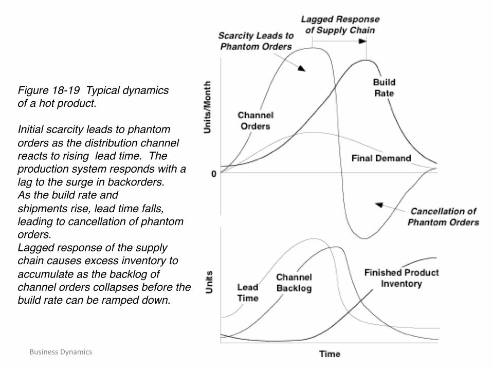
Figure 18-19 Typical dynamicsof a hot product.

Initial scarcity leads to phantom orders as the distribution channel reacts to rising lead time. The production system responds with a lag to the surge in backorders. As the build rate and shipments rise, lead time falls, leading to cancellation of phantom orders.Lagged response of the supply chain causes excess inventory to accumulate as the backlog of channel orders collapses before the build rate can be ramped down.

Business Dynamics

Figure 18-20 Causal loop diagram showing how hot products generatesurplus inventory.

Business Dynamics

Figure 18-21 Simulations of the full model compared to history for slow-moving and hot products.

TOP: Simulation of a slow-movingproduct. Sales fall short of initial projections; backlog is rapidly depletedand excess inventory accumulates.

BOTTOM: Simulation of a hot product.Strong sales lead to huge backlog, logdelays, and phantom orders by distribution channel.

When restaged production eventually shrinks delivery times, channel orders arecanceled, leading to excess inventory.

Time periods and vertical scales disguised.

Business Dynamics

Figure 18-22 Causal diagram showing Sources of synergy among lead timereduction policies.

Business Dynamics

Figure 18-23 Buildup of surplus inventory was self-reinforcing.Financial pressure to reduce inventory buildup let to more conservative Initial materials staging, increasing the chance of shortages that lead to phantom orders, aggressive late restaging of materials, and buildup of even more surplus stock, in a vicious cycle.

Business Dynamics

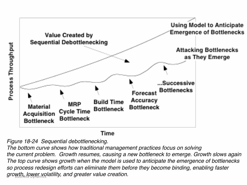
Figure 18-24 Sequential debottlenecking.The bottom curve shows how traditional management practices focus on solvingthe current problem. Growth resumes, causing a new bottleneck to emerge. Growth slows again The top curve shows growth when the model is used to anticipate the emergence of bottlenecks so process redesign efforts can eliminate them before they become binding, enabling faster growth, lower volatility, and greater value creation.

46

The End