Synthetic Aperture Radar Imaging and Motion Estimation

via Robust Principal Component Analysis

Liliana Borcea†, Thomas Callaghan†, and George Papanicolaou‡

Abstract

We consider the problem of synthetic aperture radar (SAR) imaging and motion estimation of complex

scenes. By complex we mean scenes with multiple targets, stationary and in motion. We use the

usual setup with one moving antenna emitting and receiving signals. We address two challenges: (1)

the detection of moving targets in the complex scene and (2) the separation of the echoes from the

stationary targets and those from the moving targets. Such separation allows high resolution imaging

of the stationary scene and motion estimation with the echoes from the moving targets alone. We show

that the robust principal component analysis (PCA) method which decomposes a matrix in two parts,

one low rank and one sparse, can be used for motion detection and data separation. The matrix that

is decomposed is the pulse and range compressed SAR data indexed by two discrete time variables: the

slow time, which parametrizes the location of the antenna, and the fast time, which parametrizes the

echoes received between successive emissions from the antenna. We present an analysis of the rank of the

data matrix to motivate the use of the robust PCA method. We also show with numerical simulations

that successful data separation with robust PCA requires proper data windowing. Results of motion

estimation and imaging with the separated data are presented, as well.

1 Introduction

In synthetic aperture radar (SAR), the basic problem [6, 16, 7] is to image the reflectivity supported in aset J I on the ground surface using measurements obtained with an antenna system mounted on a platformflying above it, as illustrated in Figure 1. The antenna emits periodically a probing signal f(t) and recordsthe echos D(s, t), indexed by the slow time s of the SAR platform displacement and the fast time t. Theslow time parametrizes the location ~r(s) of the platform at the instant it emits the signal, and the fast timet parametrizes the echoes received between two consecutive illuminations (0 < t < ∆s). The echoes D(s, t)are approximately, and up to a multiplicative factor, a superposition of the emitted signals f(t) time-delayedby the round-trip travel-time between the platform ~r(s) and the locations ~ρ of scatterers on the ground

τ (s, ~ρ) = 2 |~r(s)− ~ρ| /c. (1.1)

Here c is the wave speed, assumed constant and equal to the speed of light.†Computational and Applied Mathematics, Rice University, MS 134, Houston, TX 77005-1892. (borcea@caam.rice.edu and

tscallaghan@rice.edu)‡Department of Mathematics, Stanford University, Stanford, CA 94305. (papanicolalou@stanford.edu)

1

~r(s)

~ρ

J Ix

y

z

|~r(s)− ~ρ|

Figure 1: Setup for synthetic aperture imaging.

A SAR image is formed by superposing over a platform trajectory of length (aperture) a the data D(s, t)convolved with the time reversed emitted signal (matched filtered), and then backpropagated to points inthe imaging domain J I using travel times. With high bandwidth probing signals and large flight apertures,SAR is capable of generating images with roughly ten centimeter resolution at ranges of ten kilometers awayfrom the platform. Such resolution cannot be achieved for complex scenes because moving targets appearblurred and displaced in the images. Image formation should therefore be done in conjunction with targetmotion estimation. In fact, in applications such as persistent surveillance SAR, tracking and imaging themoving targets is one of the primary objectives.

Because targets may have complicated motion over lengthy data acquisition trajectories, the targets aretracked over successive small sub-apertures. Each sub-aperture corresponds to a short time interval overwhich the target is in approximate uniform translational motion. The problem is to estimate this motionfor each time interval in order to bring the small aperture images of the moving targets into focus. Then,the images are superposed to form high resolution images over larger apertures.

The existing algorithms for motion estimation fall roughly into two categories: The first is for the usualSAR setup with a single moving antenna, and the target motion is estimated from the phase modulations ofthe return echoes [2, 9, 8, 1, 21, 25, 13, 15, 18, 20, 10]. These algorithms assume that all the targets are inthe same motion, and are sensitive to the presence of strong stationary targets. The second class of methodsuses more complex antenna systems [14, 24, 23], with multiple receiver and/or transmitter antennas. Theyform a collection of images with the echoes measured by each receiver-transmitter pair, and then they usethe phase variation of the images with respect to the receiver/transmitter offsets, pixel by pixel, to extractthe target velocity.

In this paper we consider imaging and motion estimation of complex scenes with the usual SAR setup,using a single antenna. We address two challenges: (1) the detection of moving targets in the scene and (2)the separation of data in subsets of echoes from the stationary scene and echoes from the moving targets.The stationary scene can be imaged by itself after such separation, and the motion estimation can be carried

2

out on the echoes from the moving targets alone. We propose and analyze a detection and data separationapproach based on the robust principle component analysis (robust PCA) method [4]. Robust PCA isdesigned to decompose a matrix into a low rank one plus a sparse one. The main contribution of this paperis to show with analysis and numerical simulations that by appropriately pre-processing and windowing theSAR data we can decompose it into a low rank part, corresponding to the stationary scene, and a sparsepart, corresponding to the moving targets. Our theoretical and numerical study describes the rank of thepre-processed SAR data as a function of the velocity, location, and density of the scatterers. It specifiesin particular how slowly a target can move and still be distinguishable from the stationary scene. It alsoaddresses the question of proper windowing of the data for the separation with robust PCA to work.

The paper is organized as follows: We begin in section 2 with a brief description of basic SAR dataprocessing and image formation. There are two processing steps that are key to the data decomposition:pulse compression and range compression. We illustrate with numerical simulations in section 3 that robustPCA can be used for motion detection and data separation if it is complemented with proper data windowing.The analysis is in section 4. Additional numerical results on data separation, motion estimation and imagingare in section 5. We end with a summary in section 6.

2 Basic SAR data processing and image formation

The antenna emits signals that consist of a base-band waveform fB(t) modulated by a carrier frequencyνo = ωo/(2π),

f(t) = cos(ωot)fB(t). (2.2)

Its Fourier transform is

f(ω) =∫dt f(t)eiωt =

12

[fB(ω + ωo) + fB(ω − ωo)

], (2.3)

with fB(ω) supported in the interval [−πB, πB], where B is the bandwidth. The support of f(ω) is thesame interval with center shifted at ωo, and its mirror image in the negative frequencies.

Imaging relies on accurate estimation of travel times. Recall that the echoes are approximately, up tosome amplitude factors, superpositions of the emitted signals delayed by the round trip travel times betweenthe antenna and the targets in the scene. Suppose that

fB(t) = ϕ(Bt),

with ϕ a function of a dimensionless argument and compact support in the unit interval [0, 1]. Then fB(t)has the form of a pulse, and the travel times can be estimated with precision 1/B, the pulse support. Butsuch pulses are almost never used in SAR because of power limitations at the antenna [16]. The SAR echoesshould be above the antenna’s noise level, so the emitted signals should carry large power. However, theinstantaneous power at the antenna is limited, while large net power can be delivered by longer signals, suchas chirps. The problem is that the received scattered energy is spread out over the long time support ofsuch signals, making it impossible to resolve the time of arrival of different echoes. This is overcome bycompressing the long echoes, as if they were created by an incident pulse. This pulse compression amounts

3

Fast time (seconds)

Slow

tim

e (s

econ

ds)

6.7875 6.788 6.7885 6.789 6.7895 6.79x 10 5

2.5

2

1.5

1

0.5

0

0.5

1

1.5

2

2.5

Fast time (seconds)

Slow

tim

e (s

econ

ds)

1.5 1 0.5 0 0.5 1 1.5x 10 8

2.5

2

1.5

1

0.5

0

0.5

1

1.5

2

2.5

4 2 0 2 41

0.8

0.6

0.4

0.2

0

0.2

0.4

0.6

0.8

1

Slow time (seconds)

Dr(s

,0)

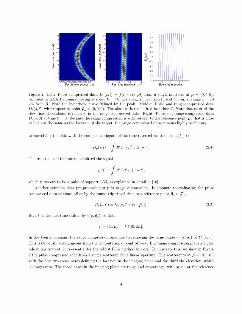
Figure 2: Left: Pulse compressed data Dp(s, t) = f(t − τ(s, ~ρ)) from a single scatterer at ~ρ = (0, 5, 0),recorded by a SAR antenna moving at speed V = 70 m/s along a linear aperture of 400 m, at range L = 10km from ~ρ. Note the hyperbolic curve defined by the peak. Middle: Pulse and range-compressed dataDr(s, t′) with respect to point ~ρo = (0, 0, 0). The abscissa is the shifted fast time t′. Note that most of theslow time dependence is removed in the range-compressed data. Right: Pulse and range-compressed dataDr(s, 0) at time t′ = 0. Because the range compression is with respect to the reference point ~ρo that is closeto but not the same as the location of the target, the range compressed data remains highly oscillatory.

to convolving the data with the complex conjugate of the time reversed emitted signal f(−t)

Dp(s, t) =∫dt′D(s, t′)f (t′ − t). (2.4)

The result is as if the antenna emitted the signal

fp(t) =∫dt′ f(t′)f (t′ − t),

which turns out to be a pulse of support 1/B, as explained in detail in [16].Another common data pre-processing step is range compression. It amounts to evaluating the pulse

compressed data at times offset by the round trip travel time to a reference point ~ρo ∈ JI,

Dr(s, t′) = Dp(s, t′ + τ(s, ~ρo)). (2.5)

Here t′ is the fast time shifted by τ(s, ~ρo), so that

t′ + τ(s, ~ρo) = t ∈ [0,∆s].

In the Fourier domain, the range compression amounts to removing the large phase ωτ(s, ~ρo) of Dp(s, ω).This is obviously advantageous from the computational point of view. But range compression plays a biggerrole in our context. It is essential for the robust PCA method to work. To illustrate this, we show in Figure2 the pulse compressed echo from a single scatterer, for a linear aperture. The scatterer is at ~ρ = (0, 5, 0),with the first two coordinates defining the location in the imaging plane and the third the elevation, whichis always zero. The coordinates in the imaging plane are range and cross-range, with origin at the reference

4

point. The range is the coordinate of ~ρ along the direction pointing from the SAR platform (at the centerof the aperture) to ~ρo. The cross-range is the coordinate of ~ρ in the direction orthogonal to the range.

We plot in Figure 2 the amplitude of Dp(s, t) as a function of s and t, and note that the location of thepeak, defined by equation (

ct

2

)2

= |~r(s)− ~ρ|2,

is a hyperbola for the linear aperture. The peak lies on some other curve in the (s, t) plane for otherapertures. The amplitude of the range compressed data is shown in the middle plot of Figure 2. Wenote that the dependence on the slow time s has been approximately removed by the range compression.Explicitly, it lies on the curve in the (s, t′) plane defined by equation

ct′

2= |~r(s)− ~ρ| − |~r(s)− ~ρo|.

This curve is close to the vertical axis t′ = 0 because ~ρ and ~ρo are close to each other,

|~ρ− ~ρo| � |~r(s)− ~ρ|, ∀s.

Consequently, the matrix with entries Dr(s, t), sampled at discrete s and t, appears to be of low rank whichsuggests that robust PCA method may be applicable. However, when we look closer at the data (right plotof Figure 2) we see that it has fast oscillations, so the rank may be higher than expected.

We work with the pulse and range compressed data from now on, and to simplify notation, we drop theprime from the shifted fast time t′. We borrow terminology from the geophysics literature and call the pulseand range compressed echoes data traces. The image is formed by superposing the traces over the aperture,and backpropagating them to the imaging points ~ρ I ∈ J I using travel times

I(~ρI)

=n/2∑

j=−n/2

Dr(sj , τ(sj , ~ρI)− τ(sj , ~ρo))

≈ 1∆s

∫ S(a)

−S(a)

dsDr(s, τ(s, ~ρ I)− τ(s, ~ρo)). (2.6)

Here sj are the discrete slow time samples in the interval [−S(a), S(a)] defining the aperture a along theflight track. The sampling is uniform, at intervals ∆s, and

2S(a) = n∆s, with n even.

Assuming a large n, that is a small ∆s, we approximate the sum in (2.6) by an integral over the aperture.When the aperture is very large, the data in (2.6) is weighted by a factor that compensates for geometrical

spreading effects over the long flight track, and thus improves the focus of the image. Here we work withsmall apertures where geometrical spreading plays no role, which is why there are no weights in the imagingfunction (2.6).

5

3 Robust PCA for motion detection and SAR data separation

We begin in section 3.1 with a brief discussion of the robust PCA method. Then, we give in section 3.2a heuristic explanation of why it makes sense to use it for motion detection and data separation. We alsoillustrate in section 3.3 the difficulties arising in the separation, and the improvements achieved by properdata windowing.

3.1 Robust PCA

The robust PCA method, introduced and analyzed in [4], applies to matrices M ∈ Rn1×n2 that are sumsof a low rank matrix Lo and a sparse matrix So. It solves a convex optimization problem called principlecomponent pursuit:

minL,S∈Rn1×n2

||L||∗ + η||S||1 (3.1)

subject to L+ S = M, (3.2)

withη =

1√max{n1, n2}

. (3.3)

Here ||L||∗ is the nuclear norm, i.e. the sum of the singular values of L, and ||S||1 is the matrix 1-norm of S.The optimization can be done for any matrix, but the point is that if M = Lo+So, with Lo low rank and Sosparse and high rank, then the principle component pursuit recovers exactly Lo and So. The analysis in [4]gives sufficient conditions under which the decomposition is exact. These conditions are bounds on the rankof Lo and the number of non-zero entries in the high rank matrix So. They are not necessary conditions,meaning that the decomposition can be achieved for a much larger class of matrices than those fulfilling theassumptions of the theorems in [4]. This is already pointed out in [4].

3.2 The structure of the matrix of range compressed SAR data

We illustrate in this section the pulse and range compressed echoes (the traces) from a complex scene. Thepoint of the illustration is to show that typically, the sampled traces from the stationary scene form a lowrank matrix, whereas those from moving targets give a high rank but sparse matrix. We refer to section 5for the description of the setup of the numerical simulations used to produce the results presented here andin the next section.

Let M be the matrix with entries given by the data traces sampled at the discrete slow and fast times

Mjl = Dr(sj , tl), (3.4)

wheresj = j∆s, j = −n/2, . . . , n/2, (3.5)

andtl = l∆t, l = −m/2, . . . ,m/2. (3.6)

6

Fast time (seconds)

Slow

time

(sec

onds

)

4 2 0 2 4x 10 7

2

1.5

1

0.5

0

0.5

1

1.5

2

Fast time (seconds)Sl

owtim

e (s

econ

ds)

4 2 0 2 4x 10 7

2

1.5

1

0.5

0

0.5

1

1.5

2

Fast time (seconds)

Slow

time

(sec

onds

)

4 2 0 2 4x 10 7

2

1.5

1

0.5

0

0.5

1

1.5

2

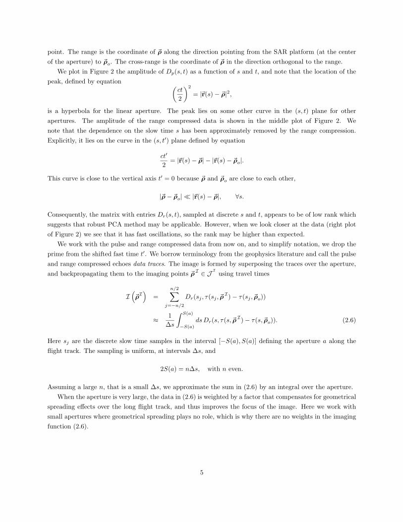
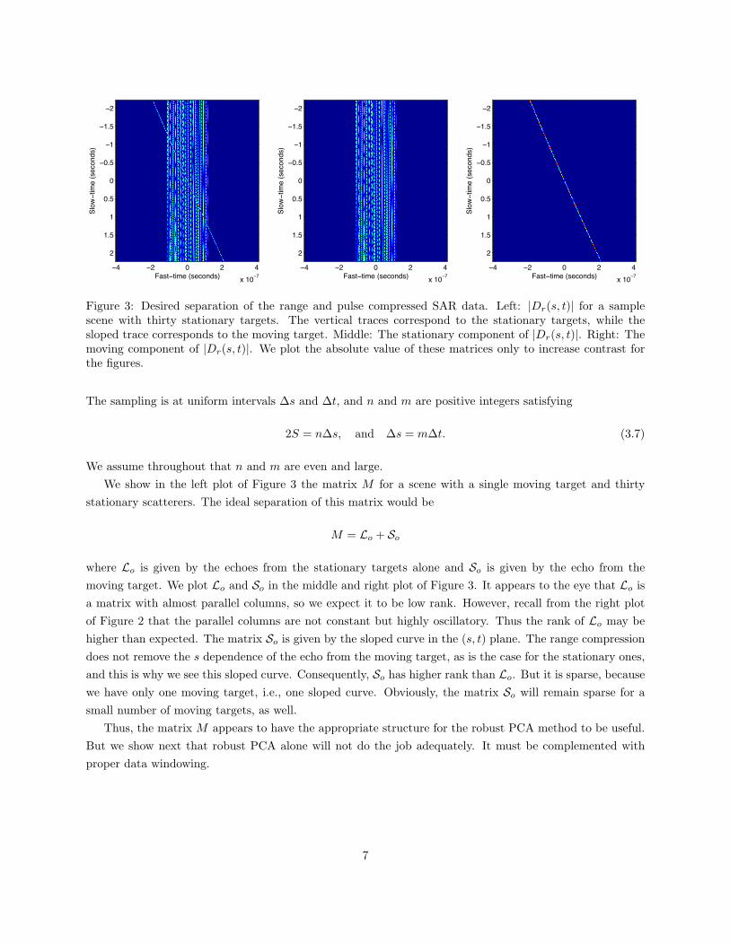
Figure 3: Desired separation of the range and pulse compressed SAR data. Left: |Dr(s, t)| for a samplescene with thirty stationary targets. The vertical traces correspond to the stationary targets, while thesloped trace corresponds to the moving target. Middle: The stationary component of |Dr(s, t)|. Right: Themoving component of |Dr(s, t)|. We plot the absolute value of these matrices only to increase contrast forthe figures.

The sampling is at uniform intervals ∆s and ∆t, and n and m are positive integers satisfying

2S = n∆s, and ∆s = m∆t. (3.7)

We assume throughout that n and m are even and large.We show in the left plot of Figure 3 the matrix M for a scene with a single moving target and thirty

stationary scatterers. The ideal separation of this matrix would be

M = Lo + So

where Lo is given by the echoes from the stationary targets alone and So is given by the echo from themoving target. We plot Lo and So in the middle and right plot of Figure 3. It appears to the eye that Lo isa matrix with almost parallel columns, so we expect it to be low rank. However, recall from the right plotof Figure 2 that the parallel columns are not constant but highly oscillatory. Thus the rank of Lo may behigher than expected. The matrix So is given by the sloped curve in the (s, t) plane. The range compressiondoes not remove the s dependence of the echo from the moving target, as is the case for the stationary ones,and this is why we see this sloped curve. Consequently, So has higher rank than Lo. But it is sparse, becausewe have only one moving target, i.e., one sloped curve. Obviously, the matrix So will remain sparse for asmall number of moving targets, as well.

Thus, the matrix M appears to have the appropriate structure for the robust PCA method to be useful.But we show next that robust PCA alone will not do the job adequately. It must be complemented withproper data windowing.

7

Fast time (seconds)

Slow

tim

e (s

econ

ds)

4 3 2 1 0 1 2 3 4x 10 7

2

1.5

1

0.5

0

0.5

1

1.5

20

0.1

0.2

0.3

0.4

0.5

0.6

0.7

0.8

0.9

1

Fast time (seconds)

Slow

tim

e (s

econ

ds)

4 3 2 1 0 1 2 3 4x 10 7

2

1.5

1

0.5

0

0.5

1

1.5

20

0.1

0.2

0.3

0.4

0.5

0.6

0.7

0.8

0.9

1

Fast time (seconds)

Slow

tim

e (s

econ

ds)

4 3 2 1 0 1 2 3 4x 10 7

2

1.5

1

0.5

0

0.5

1

1.5

250

45

40

35

30

25

20

15

10

5

0

Fast time (seconds)

Slow

tim

e (s

econ

ds)

6 4 2 0 2 4 6x 10 8

2

1.5

1

0.5

0

0.5

1

1.5

20

0.1

0.2

0.3

0.4

0.5

0.6

0.7

0.8

0.9

1

Fast time (seconds)

Slow

tim

e (s

econ

ds)

6 4 2 0 2 4 6x 10 8

2

1.5

1

0.5

0

0.5

1

1.5

20

0.1

0.2

0.3

0.4

0.5

0.6

0.7

0.8

0.9

1

Fast time (seconds)

Slow

tim

e (s

econ

ds)

6 4 2 0 2 4 6x 10 8

2

1.5

1

0.5

0

0.5

1

1.5

250

45

40

35

30

25

20

15

10

5

0

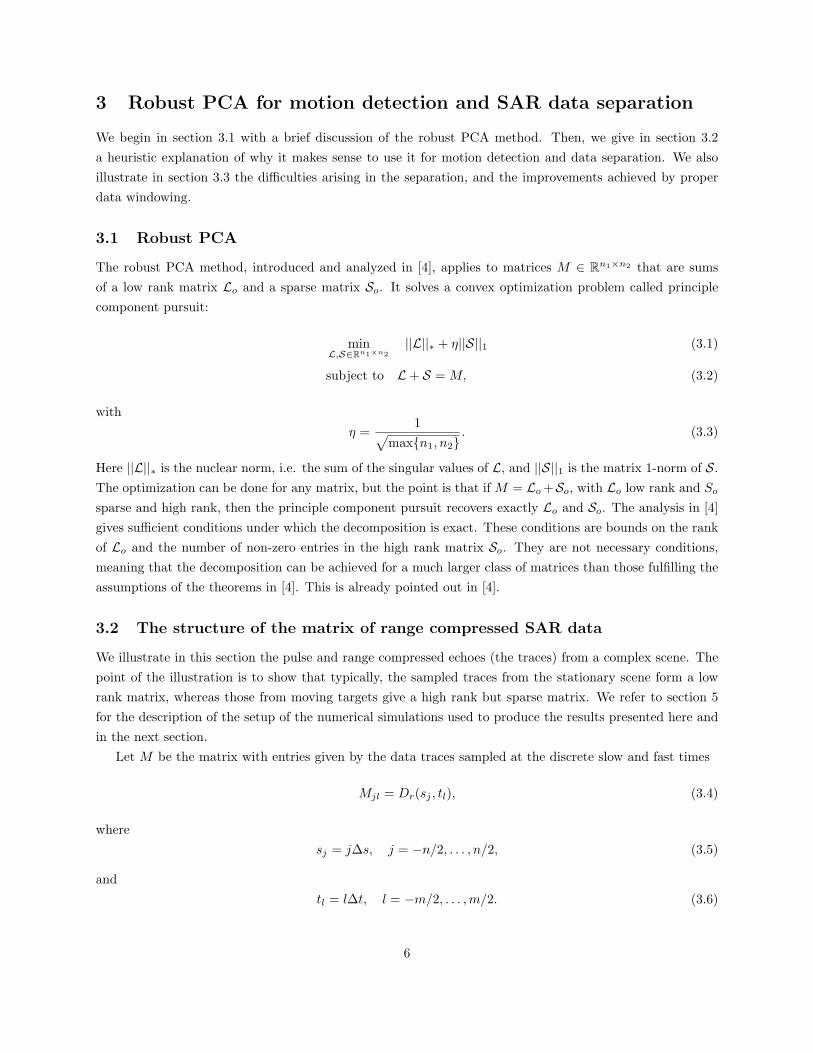
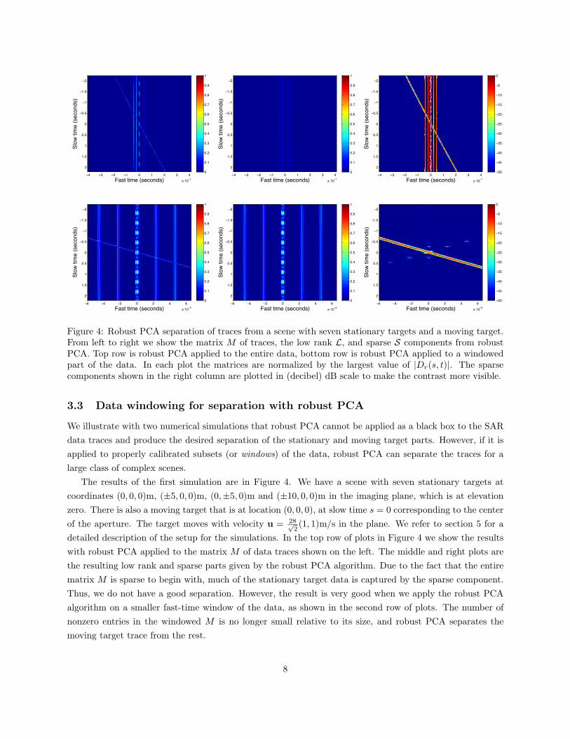
Figure 4: Robust PCA separation of traces from a scene with seven stationary targets and a moving target.From left to right we show the matrix M of traces, the low rank L, and sparse S components from robustPCA. Top row is robust PCA applied to the entire data, bottom row is robust PCA applied to a windowedpart of the data. In each plot the matrices are normalized by the largest value of |Dr(s, t)|. The sparsecomponents shown in the right column are plotted in (decibel) dB scale to make the contrast more visible.

3.3 Data windowing for separation with robust PCA

We illustrate with two numerical simulations that robust PCA cannot be applied as a black box to the SARdata traces and produce the desired separation of the stationary and moving target parts. However, if it isapplied to properly calibrated subsets (or windows) of the data, robust PCA can separate the traces for alarge class of complex scenes.

The results of the first simulation are in Figure 4. We have a scene with seven stationary targets atcoordinates (0, 0, 0)m, (±5, 0, 0)m, (0,±5, 0)m and (±10, 0, 0)m in the imaging plane, which is at elevationzero. There is also a moving target that is at location (0, 0, 0), at slow time s = 0 corresponding to the centerof the aperture. The target moves with velocity u = 28√

2(1, 1)m/s in the plane. We refer to section 5 for a

detailed description of the setup for the simulations. In the top row of plots in Figure 4 we show the resultswith robust PCA applied to the matrix M of data traces shown on the left. The middle and right plots arethe resulting low rank and sparse parts given by the robust PCA algorithm. Due to the fact that the entirematrix M is sparse to begin with, much of the stationary target data is captured by the sparse component.Thus, we do not have a good separation. However, the result is very good when we apply the robust PCAalgorithm on a smaller fast-time window of the data, as shown in the second row of plots. The number ofnonzero entries in the windowed M is no longer small relative to its size, and robust PCA separates themoving target trace from the rest.

8

Fast time (seconds)

Slow

tim

e (s

econ

ds)

4 3 2 1 0 1 2 3 4x 10 7

2

1.5

1

0.5

0

0.5

1

1.5

20

0.1

0.2

0.3

0.4

0.5

0.6

0.7

0.8

0.9

1

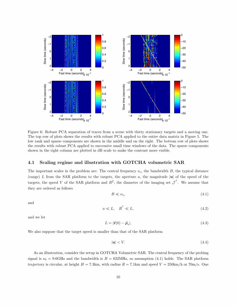
Figure 5: SAR scene with thirty stationary targets and a moving one.

In Figure 6 we show the results for a scene with thirty stationary targets and a moving one. The datatraces from this scene are displayed in Figure 5. The moving target is as in the previous example. Thepoint of the simulation is to show that when we work in a large fast time window the traces from all thestationary targets may no longer form a low rank matrix. The top row of plots in Figure 6 shows that thesparse component of the matrix M , as returned by the robust PCA algorithm, has a large residual part fromthe stationary targets. The much improved results in the bottom are obtained by applying robust PCAon successive small fast time windows of the data, and then reassembling the separated traces. To give anidea of the size of the windows, the matrix M has dimensions n = 296 by m = 16, 384. The matrices arewindowed in fast-time and are of size 296× 450.

The two examples given above show that data windowing plays an important role in achieving a successfuldata separation with robust PCA. The last simulation also illustrates the role of robust PCA in the detectionof the moving target. While the trace from this target is faint and difficult to distinguish from the othersover most of the fast time interval in Figure 5, it is clearly visible in Figure 6 after the processing of thetraces with robust PCA.

4 Analysis of rank of the matrix of SAR data traces

We present here an analysis of the rank of the matrix of SAR data traces for simple scenes with one or twotargets. The goal is to understand how the rank depends on the position of the targets and their velocity.We limit the analysis to at most two targets to get a simple structure of the matrix MMT , for which we cancalculate the rank almost explicitly. The numerical results presented above and in section 5 show that thedata separation works for complex scenes, with many stationary targets.

We begin in section 4.1 with the scaling regime used in the analysis. We illustrate it with the GOTCHAVolumetric SAR data set [5] for X-band surveillance SAR. The model of the matrix M is given in section4.2. We analyze its rank in section 4.3 for a single target, and in section 4.4 for two targets. We end with abrief discussion in section 4.5.

9

Fast time (seconds)

Slow

tim

e (s

econ

ds)

4 2 0 2 4x 10 7

2

1

0

1

2

Fast time (seconds)

Slow

tim

e (s

econ

ds)

4 2 0 2 4x 10 7

2

1

0

1

2

Fast time (seconds)

Slow

tim

e (s

econ

ds)

4 2 0 2 4x 10 7

2

1

0

1

2

Fast time (seconds)Sl

ow ti

me

(sec

onds

)

4 2 0 2 4x 10 7

2

1

0

1

2 50

40

30

20

10

0

50

40

30

20

10

0

0

0.2

0.4

0.6

0.8

1

0

0.2

0.4

0.6

0.8

1

Figure 6: Robust PCA separation of traces from a scene with thirty stationary targets and a moving one.The top row of plots shows the results with robust PCA applied to the entire data matrix in Figure 5. Thelow rank and sparse components are shown in the middle and on the right. The bottom row of plots showsthe results with robust PCA applied to successive small time windows of the data. The sparse componentsshown in the right column are plotted in dB scale to make the contrast more visible.

4.1 Scaling regime and illustration with GOTCHA volumetric SAR

The important scales in the problem are: The central frequency νo, the bandwidth B, the typical distance(range) L from the SAR platform to the targets, the aperture a, the magnitude |u| of the speed of thetargets, the speed V of the SAR platform and RI , the diameter of the imaging set J I . We assume thatthey are ordered as follows

B � νo, (4.1)

anda� L, R

I� L, (4.2)

and we letL = |~r(0)− ~ρo|. (4.3)

We also suppose that the target speed is smaller than that of the SAR platform

|u| < V. (4.4)

As an illustration, consider the setup in GOTCHA Volumetric SAR. The central frequency of the probingsignal is ν0 = 9.6GHz and the bandwidth is B = 622MHz, so assumption (4.1) holds. The SAR platformtrajectory is circular, at height H = 7.3km, with radius R = 7.1km and speed V = 250km/h or 70m/s. One

10

circular degree of trajectory is 124m. The pulse repetition rate is 117 per degree, which means that a pulseis sent every 1.05m, and ∆s = 0.015s. A typical distance to a target is L = 10km and we consider imagingdomains of radius R

Iof at most 50m, so assumptions (4.2) hold. The target speed is |u| ∼ 100km/h or

28m/s, so it satisfies (4.4).For a stationary target we obtain from basic resolution theory (for single small aperture imaging) that

the range can be estimated with precision c/B = 48cm, and the cross range resolution is λ0L/a = 2.5m,with one degree aperture a and central wavelength λ0 = 3cm. The image of a moving target is out of focusunless we estimate its velocity and compensate for the motion in the imaging function.

4.2 Data model

Our model of the data assumes that the scatterers lying on the imaging surface behave like point targets.We neglect any interaction between the scatterers, meaning that we make the single scattering, Born ap-proximation. The pulse and range compressed data is approximated by

Dr(s, t) ≈N∑q=1

σq(ωo)(4π|~r(s)− ~ρq(s)|)2

fp(t− (τ(s, ~ρq(s))− τ(s, ~ρo))), (4.5)

in the case of N targets at locations

~ρq(s) = (ρq(s), 0), q = 1, . . . , N,

with reflectivity σq(ωo). Here we used the so-called stop-start approximation which neglects the displacementof the targets during the round trip travel time. This is justified in radar because the waves travel at thespeed of light that is many orders of magnitude larger than the speed of the targets. We refer to [2] for aderivation of the model (4.5) in the scaling regime described above.

Because of our scaling assumptions (4.2), we can approximate the amplitude factors as

14π|~r(s)− ~ρq(s)|

≈ 14πL

,

and obtain the simpler model

Dr(s, t) =(

14πL

)2 N∑q=1

σqfp(t−∆τ(s, ~ρq(s))), (4.6)

where we let∆τ(s, ~ρ(s)) = τ(s, ~ρ(s))− τ(s, ~ρ0). (4.7)

We assume henceforth, for simplicity, that the targets are identical

σq = σ, q = 1, . . . , N,

11

and writeDr(s, t) ≈

σ(ωo)(4πL)2

M(s, t), (4.8)

with

M(s, t) =N∑q=1

fp(t−∆τ(s, ~ρq(s))). (4.9)

The matrix of traces analyzed below is given by discrete samples of (4.9),

Mjl =M(sj−n2−1, tl−1

), j = 1, . . . , n+ 1, l = 1, . . . ,m+ 1, (4.10)

with slow times sj and fast times tl defined in (3.5) and (3.6). We also take for convenience a compressedpulse given by a Gaussian modulated by a cosine at the central frequency,

fp(t) = cos(ωot)e−B2t2/2. (4.11)

4.3 Analysis of rank of the data traces for one target

In the case of one target at location ~ρ(s) = (ρ(s), 0), the entries of matrix (4.10) are given by

Mjl = cos [ωo(t−∆τ(s, ~ρ(s)))] exp[−B

2

2(t−∆τ(s, ~ρ(s)))2

], (4.12)

with ∆τ defined by (4.7). The target is moving at speed ~u = (u, 0), so we have that

~ρ(s) = ~ρ + s ~u, |s| ≤ S(a), (4.13)

where we let~ρ := ~ρ(0)

be the location of the target at the time s = 0, corresponding to the center of the aperture.We study the rank of M , which is equivalent to studying the rank of the symmetric, square matrix

C ∈ R(n+1)×(n+1), with entries given by

Cj,l = C(sj−n2−1, sl−n2−1

), j, l = 1, . . . , n+ 1, (4.14)

in terms of the function

C(s, s′) =m/2∑

q=−m/2

Dr(s, tq)Dr(s′, tq) ≈1

∆t

∫ ∞−∞

dt Dr(s, t)Dr(s, t). (4.15)

Here we used the assumption that ∆t is small enough to approximate the Riemann sum over q by the integralover t. Because the traces Dr(s, t) vanish for |t| > ∆s/2, we extended the integral to the whole real line.

We obtain after a calculation given in appendix A that if the aperture a is small enough, the matrix Chas a Toeplitz structure.

12

Proposition 1 Assuming that the Fresnel number a2

λoLis bounded by

a2

λoL� min

{L

RI,V

|~u|

}, (4.16)

the matrix C is approximately Toeplitz, with entries given by

C(s, s′) ≈√π

2B∆tcos [ωoα(s− s′)] exp

[− (Bα)2(s− s′)2

4

]. (4.17)

The dimensionless parameter α depends linearly on the velocity in the range direction and the cross-rangeoffset of the target with respect to the reference point ~ρo. It is given by

α =2~u · ~mo

c− 2V~t · Po(~ρ− ~ρo)

cL+

2~u · Po(~ρ− ~ρo)cL

, (4.18)

with ~mo the unit vector pointing in the range direction from the center ~r(0) of the aperture

~mo =~r(0)− ~ρo|~r(0)− ~ρo|

, (4.19)

and Po the orthogonal projectionPo = I − ~mo ~mT

o . (4.20)

The unit vector ~t is defined byd~r(0)ds

= V~t. (4.21)

It is tangential to the flight track, at the center of the aperture.

Slow time (seconds)

Slow

tim

e (s

econ

ds)

0 0.5 1 1.5 2 2.5 3 3.5 4

0

0.5

1

1.5

2

2.5

3

3.5

4

Figure 7: The matrix C for one stationary target at ~ρ = (0, 15, 0)m. The reference point is ~ρo = ~0. Theaperture is 310m, the range L = 10km and the central wavelength is λo = 3cm. The plot shows that thematrix is essentially constant along the diagonals, it is approximately Toeplitz.

As an illustration, we plot in Figure 7 the matrix C for an aperture a = 310m, in the GOTCHA regimewith central wavelength λo = 3cm and range L = 10km. We have a stationary target at ~ρ = (0, 15, 0)m, and

13

Fast time (seconds)

Slow

tim

e (s

econ

ds)

5 0 5x 10 9

2

1.5

1

0.5

0

0.5

1

1.5

2

Fast time (seconds)

Slow

tim

e (s

econ

ds)

6 5.5 5 4.5 4 3.5x 10 8

2

1.5

1

0.5

0

0.5

1

1.5

2

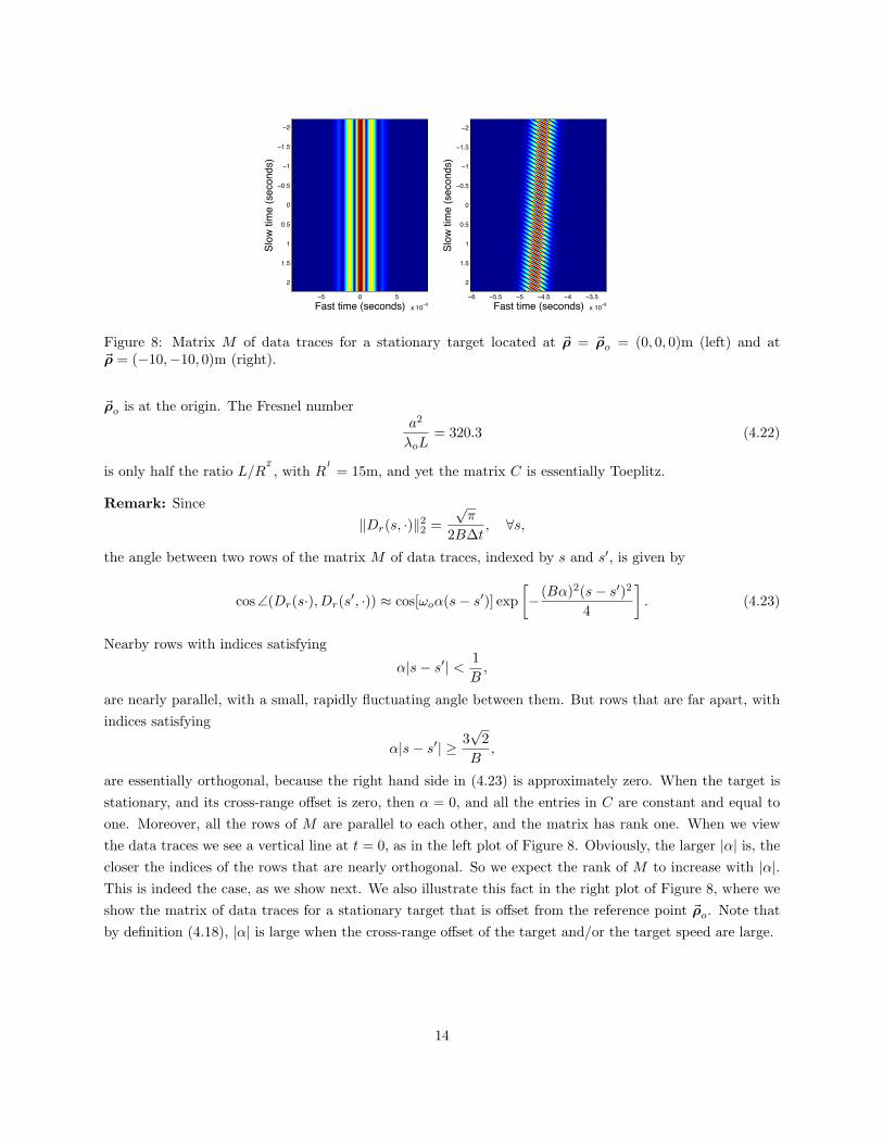
Figure 8: Matrix M of data traces for a stationary target located at ~ρ = ~ρo = (0, 0, 0)m (left) and at~ρ = (−10,−10, 0)m (right).

~ρo is at the origin. The Fresnel numbera2

λoL= 320.3 (4.22)

is only half the ratio L/RI, with R

I

= 15m, and yet the matrix C is essentially Toeplitz.

Remark: Since‖Dr(s, ·)‖22 =

√π

2B∆t, ∀s,

the angle between two rows of the matrix M of data traces, indexed by s and s′, is given by

cos ∠(Dr(s·), Dr(s′, ·)) ≈ cos[ωoα(s− s′)] exp[− (Bα)2(s− s′)2

4

]. (4.23)

Nearby rows with indices satisfying

α|s− s′| < 1B,

are nearly parallel, with a small, rapidly fluctuating angle between them. But rows that are far apart, withindices satisfying

α|s− s′| ≥ 3√

2B

,

are essentially orthogonal, because the right hand side in (4.23) is approximately zero. When the target isstationary, and its cross-range offset is zero, then α = 0, and all the entries in C are constant and equal toone. Moreover, all the rows of M are parallel to each other, and the matrix has rank one. When we viewthe data traces we see a vertical line at t = 0, as in the left plot of Figure 8. Obviously, the larger |α| is, thecloser the indices of the rows that are nearly orthogonal. So we expect the rank of M to increase with |α|.This is indeed the case, as we show next. We also illustrate this fact in the right plot of Figure 8, where weshow the matrix of data traces for a stationary target that is offset from the reference point ~ρo. Note thatby definition (4.18), |α| is large when the cross-range offset of the target and/or the target speed are large.

14

4.3.1 Asymptotic characterization of the rank

Because matrix C is Toeplitz and large, we can use the asymptotic Szego theory [17, 3] to estimate its rank.To do so, let us define the sequence {cj}j∈Z with entries

cj =√π

2B∆te−

(ξj)2

4 cos(γj), ξ = B|α|∆s, (4.24)

and where γ ∈ (−π, π) is defined by

γ = [(ω0α∆s+ π) mod 2π]− π. (4.25)

A finite set of this sequence, for indices |j| ≤ n, defines approximately the diagonals of the matrix C,

Cj,l ≈ cj−l, j, l = 1, . . . , n+ 1. (4.26)

Since multiplication of a large Toeplitz matrix with a vector is approximately a convolution, and sinceconvolutions are diagonalized by the Fourier transform, it is not surprising that the spectrum of C is definedin terms of the symbol Q(θ), the coefficients of the Fourier series of (4.24),

Q(θ) =∞∑

j=−∞cje

ijθ, θ ∈ (−π, π). (4.27)

With this symbol, we can characterize asymptotically in the limit n→∞ the rank of C, using Szego’s firstlimit theorem [3], that gives

limn→∞

N (n;β1, β2)n+ 1

=1

2π

∫ π

−π1[β1,β2](Q(θ))dθ. (4.28)

Here 1[β1,β2] is the indicator function of the interval [β1, β2] and N (n;β1, β2) is the number of eigenvalues ofC that lie in this interval.

We show in appendix B that the symbol is given approximately by

Q(θ) ≈ π

2B∆tξ

{exp

[− (θ − γ)2

ξ2

]+ exp

[− (θ + γ)2

ξ2

]}. (4.29)

We use this result and (4.28) to obtain an asymptotic estimate of the essential rank, defined by

rank [C] := N (n; ε‖Q‖∞,∞) , ‖Q‖∞ = supθ∈(−π,π)

|Q(θ)|. (4.30)

Here 0 < ε � 1 is a small threshold parameter, and ‖Q‖∞ is of the order of the largest singular value ofC. It follows from the Szego theory [17, 3] that this singular value is given by the maximum of the symbol,

15

0 5 10 15 20 25 300

5

10

15

20

25

Cross Range

Ran

k

Estimated RankComputed Rank

(a) Stationary

0 5 10 150

50

100

150

200

250

300

Range Velocity

Ran

k

Estimated RankComputed Rank

(b) Moving

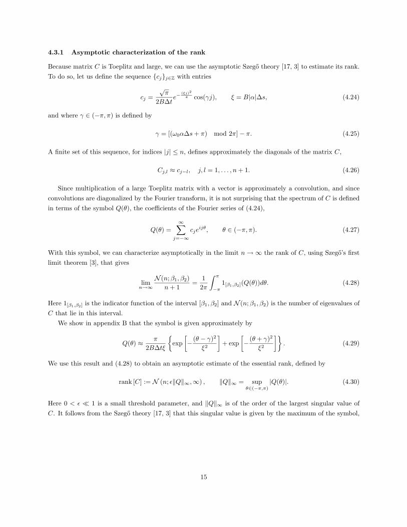
Figure 9: Comparison of the computed and estimated rank of C for a single target. Left: Stationary targetat various cross-range positions. Right: Moving target with various velocities.

which is of the order of π/(2B∆tξ). We obtain that for n� 1,

rank [C]n+ 1

≈ 12π

∫ π

−π1[ε‖Q‖∞,∞)(Q(θ))dθ

= min

(2|α|B∆s

√log 1/ε

π, 1

), (4.31)

where the last equality follows from direct calculation.As an illustration, we show with green in Figure 9a the computed rank of the matrix C for a single

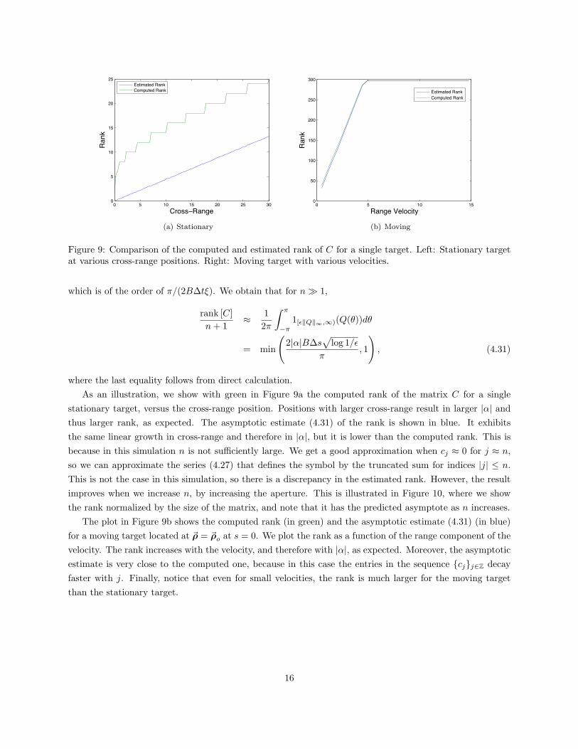
stationary target, versus the cross-range position. Positions with larger cross-range result in larger |α| andthus larger rank, as expected. The asymptotic estimate (4.31) of the rank is shown in blue. It exhibitsthe same linear growth in cross-range and therefore in |α|, but it is lower than the computed rank. This isbecause in this simulation n is not sufficiently large. We get a good approximation when cj ≈ 0 for j ≈ n,so we can approximate the series (4.27) that defines the symbol by the truncated sum for indices |j| ≤ n.This is not the case in this simulation, so there is a discrepancy in the estimated rank. However, the resultimproves when we increase n, by increasing the aperture. This is illustrated in Figure 10, where we showthe rank normalized by the size of the matrix, and note that it has the predicted asymptote as n increases.

The plot in Figure 9b shows the computed rank (in green) and the asymptotic estimate (4.31) (in blue)for a moving target located at ~ρ = ~ρo at s = 0. We plot the rank as a function of the range component of thevelocity. The rank increases with the velocity, and therefore with |α|, as expected. Moreover, the asymptoticestimate is very close to the computed one, because in this case the entries in the sequence {cj}j∈Z decayfaster with j. Finally, notice that even for small velocities, the rank is much larger for the moving targetthan the stationary target.

16

0 20 40 60 80 100 1200.02

0.025

0.03

0.035

0.04

0.045

0.05

0.055

0.06

0.065

Aperture Length (seconds)

Ran

k/(n

+1)

Figure 10: Convergence of the rank of C normalized by the size (n+ 1). The blue line is the computed valueand the green line is the asymptotic estimate.

4.4 Analysis of the rank of the data traces for two targets

In the case of two targets at locations ~ρj(s) for j = 1, 2, the entries of the matrix M follow from equations(4.9) and (4.10),

Mjl =2∑j=1

cos[ωo(t−∆τ(s, ~ρj(s)))

]exp

[−B

2

2(t−∆τ(s, ~ρj(s)))

2

]. (4.32)

We take for simplicity the case of two stationary targets

~ρj(s) = ~ρj := ~ρj(0), j = 1, 2.

Extensions to moving targets with speeds ~u1 and ~u2 are straightforward. They amount to redefining theparameters α1 and α2 defined below by adding two linear terms in the target velocity, as in equation (4.18).

The expression of matrix C = MMT is given in the following proposition. It is obtained with a calculationthat is similar to that in appendix A, using the same assumption on the Fresnel number as in Proposition 1.

Proposition 2 Assume that the Fresnel number satisfies the bound (4.16), with ~u = 0 since the targets arestationary. The matrix C has entries defined by the function

C(s, s′) ≈√π

2B∆t

2∑j=1

cos[ωoαj(s− s′)] exp[− (Bαj)2(s− s′)2

4

]

+ cos[ωo(α1s− α2s′ + β)] exp

[−B

2(α1s− α2s′ + β)2

4

](4.33)

+ cos[ωo(α1s′ − α2s+ β)] exp

[−B

2(α1s′ − α2s+ β)2

4

]},

17

sampled at the discrete slow times. Here we let

αj = −2V~t · Po(~ρj − ~ρo)

cL, (4.34)

and

β =2c

2∑j=1

(−1)j{~mo · (~ρj − ~ρo) +

[ ~mo · (~ρj − ~ρo)]2

2L

}. (4.35)

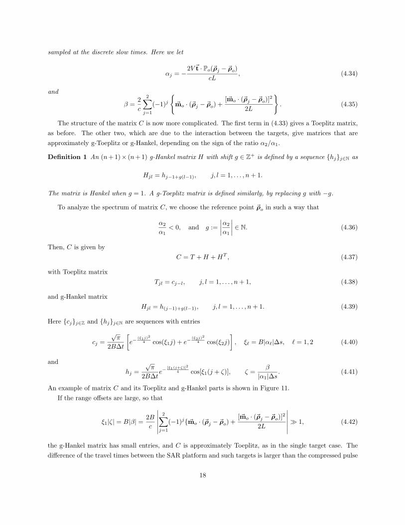
The structure of the matrix C is now more complicated. The first term in (4.33) gives a Toeplitz matrix,as before. The other two, which are due to the interaction between the targets, give matrices that areapproximately g-Toeplitz or g-Hankel, depending on the sign of the ratio α2/α1.

Definition 1 An (n+ 1)× (n+ 1) g-Hankel matrix H with shift g ∈ Z+ is defined by a sequence {hj}j∈N as

Hjl = hj−1+g(l−1), j, l = 1, . . . , n+ 1.

The matrix is Hankel when g = 1. A g-Toeplitz matrix is defined similarly, by replacing g with −g.

To analyze the spectrum of matrix C, we choose the reference point ~ρo in such a way that

α2

α1< 0, and g :=

∣∣∣∣α2

α1

∣∣∣∣ ∈ N. (4.36)

Then, C is given byC = T +H +HT , (4.37)

with Toeplitz matrixTjl = cj−l, j, l = 1, . . . , n+ 1, (4.38)

and g-Hankel matrixHjl = h(j−1)+g(l−1), j, l = 1, . . . , n+ 1. (4.39)

Here {cj}j∈Z and {hj}j∈N are sequences with entries

cj =√π

2B∆t

[e−

(ξ1j)2

4 cos(ξ1j) + e−(ξ2j)

2

4 cos(ξ2j)], ξ` = B|α`|∆s, ` = 1, 2 (4.40)

andhj =

√π

2B∆te−

[ξ1(j+ζ)]2

4 cos[ξ1(j + ζ)], ζ =β

|α1|∆s. (4.41)

An example of matrix C and its Toeplitz and g-Hankel parts is shown in Figure 11.If the range offsets are large, so that

ξ1|ζ| = B|β| = 2Bc

∣∣∣∣∣∣2∑j=1

(−1)j{ ~mo · (~ρj − ~ρo) +[ ~mo · (~ρj − ~ρo)]2

2L

∣∣∣∣∣∣� 1, (4.42)

the g-Hankel matrix has small entries, and C is approximately Toeplitz, as in the single target case. Thedifference of the travel times between the SAR platform and such targets is larger than the compressed pulse

18

Toeplitz Component

Slow time (seconds)

Slow

tim

e (s

econ

ds)

0 1 2 3 4

0

0.5

1

1.5

2

2.5

3

3.5

4

g Hankel Component

Slow time (seconds)Sl

ow ti

me

(sec

onds

)0 1 2 3 4

0

0.5

1

1.5

2

2.5

3

3.5

4

g Hankel Transpose

Slow time (seconds)

Slow

tim

e (s

econ

ds)

0 1 2 3 4

0

0.5

1

1.5

2

2.5

3

3.5

4

Matrix C

Slow time (seconds)

Slow

tim

e (s

econ

ds)

0 1 2 3 4

0

0.5

1

1.5

2

2.5

3

3.5

4

Figure 11: Components of matrix C for two stationary targets located at ~ρ1 = (0.15, 15, 0)m and ~ρ2 =(−0.15,−5, 0)m. On the left we show the Toeplitz part T . The next two plots show the g-Hankel part Hand its transpose HT . The right plot shows the sum, i.e., the matrix C.

width, and their interaction in (4.33) is negligible. If the range offsets are small, the structure of the matrixC is as in equation (4.37), and the estimate of its rank follows from the recent results in [19, 11, 12]. Theysay that the g-Hankel terms H +HT have a negligible effect on the rank in the limit n→∞. See appendixC for more details. Thus, in either case, the rank estimate of C is given by equation (4.28), in terms of thesymbol Q(θ) defined by (4.27), using the sequence {cj}j∈Z with entries (4.40).

Explicitly, the symbol is given by

Q(θ) ≈ π

2B∆tξ1

[e− (θ−γ1)2

ξ21 + e− (θ+γ1)2

ξ21

]+

π

2B∆tξ2

[e− (θ−γ2)2

ξ22 + e− (θ+γ2)2

ξ22

], (4.43)

with γj ∈ (−π, π) defined byγj = [(ω0αj∆s+ π) mod 2π]− π, (4.44)

for j = 1, 2, and the rank is given by

rank [C] ≈ (n+ 1)2π

∫ π

−π1[ε‖Q‖∞,∞)(Q(θ))dθ. (4.45)

Let us remark that we can always bound the rank of the matrix C using the sub-additivity property ofrank. The analysis presented above gives asymptotic estimates of the rank for simple scenes with one ortwo targets. The analysis extends directly to scenes with N > 2 targets that are pairwise well separated inrange, as defined in (4.42), because the matrix C is approximately Toeplitz. Its rank is as in (4.45), withsymbol Q(θ) defined by an equation similar to (4.43 ), with N terms. The sub-additivity bound becomes anasymptotic estimate of the rank in such cases, as long as the targets are at similar cross-ranges. When thetargets are close in cross-range, the rank is smaller than the sum of the ranks of the matrices correspondingto each scatterer, as explained in the next section.

19

Fast time (seconds)

Slow

tim

e (s

econ

ds)

2 1 0 1 2x 10 8

2

1.5

1

0.5

0

0.5

1

1.5

2

Fast time (seconds)

Slow

tim

e (s

econ

ds)

2 1 0 1 2x 10 8

2

1.5

1

0.5

0

0.5

1

1.5

2

Fast time (seconds)

Slow

tim

e (s

econ

ds)

5 0 5 10x 10 9

2

1.5

1

0.5

0

0.5

1

1.5

2

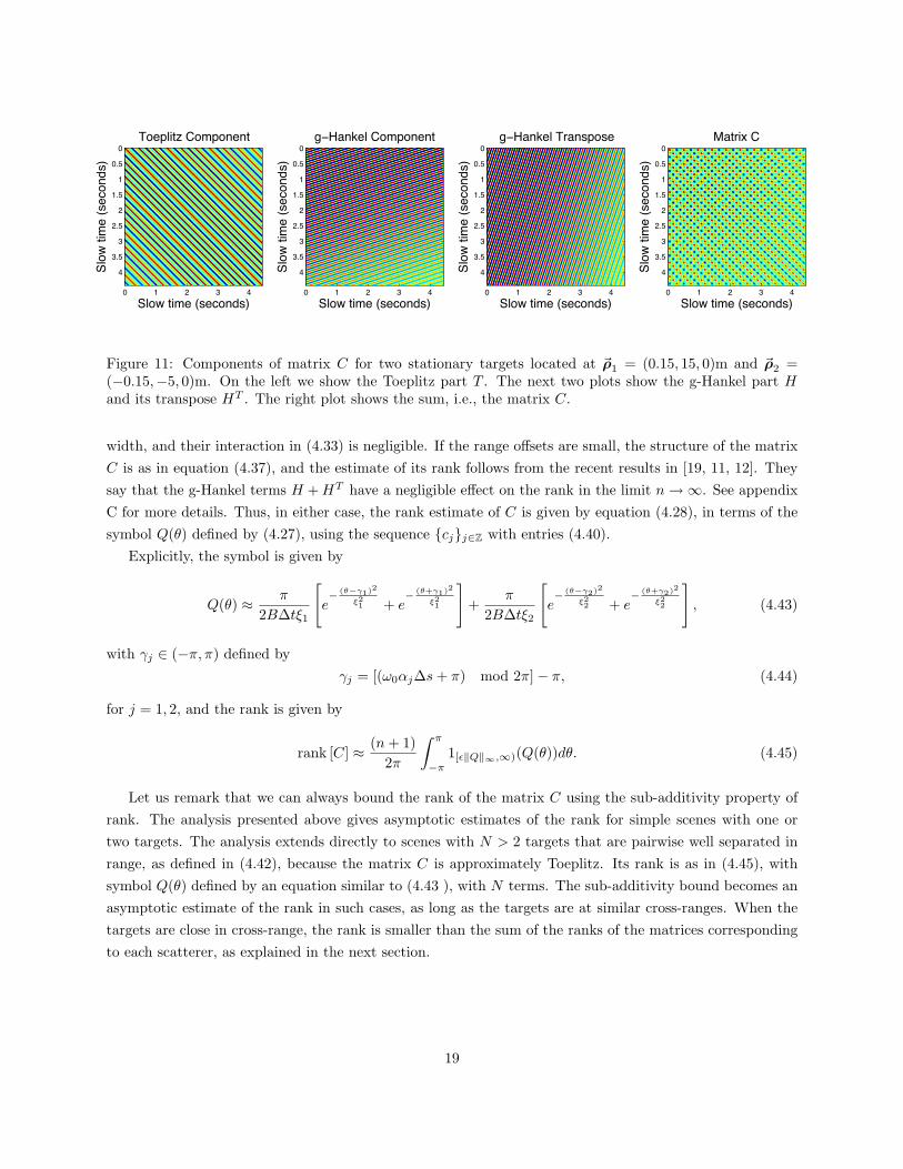
Figure 12: Data traces from two stationary targets. Left: the targets are at positions ~ρ1 = (2, 5, 0)mand ~ρ2 = (−2, 15, 0)m. Middle: ~ρ1 = (2, 5, 0)m and ~ρ2 = (−2, 5, 0)m. Right: ~ρ1 = (0.15, 5, 0)m and~ρ2 = (−0.15, 15, 0)m.

4.4.1 Illustration

We compare in Figure 13 the computed and estimated rank for two stationary targets. The results on theleft are for one target fixed at location ~ρ1 = (5, 5, 0)m. We vary the location of the other target between(−5, 0.01, 0)m and (−5, 30, 0)m. The range separation is 10m, so that B|β| = 41.47, and the g-Hankel matrixH has negligible entries. The results on the right are for one target at ~ρ1 = (0.15, 5, 0)m and the locationof the other varying between (−0.15, 0.01, 0)m to (−0.15, 30, 0)m. The range separation is 0.3m, so thatB|β| = 1.24, and the g-Hankel matrix H is no longer negligible. We see that in spite of H being neglible ornot, the rank of matrix C behaves essentially the same, as predicted by the asymptotic theory. This wouldbe difficult to guess by just looking at the data traces displayed in Figure 12.

The computed and the estimated ranks grow at the same rate with the cross range of the second target,i.e., with |α2|. The growth is monotone except in the vicinity of the local minimum corresponding to thetargets having exactly the same cross-range. In this special configuration α1 = α2, and therefore ξ1 = ξ2.The symbol (4.43) simplifies to

Q(θ) ≈ π

B∆tξ1

[e− (θ−γ1)2

ξ21 + e− (θ+γ1)2

ξ21

],

and it exceeds the threshold ε‖Q‖∞ for θ in a smaller subset of (−π, π), than in the general case with ξ1 6= ξ2.The rank is defined by the size of this set, so it should have a minimum as observed in Figure ??.

Similar to the result in Figure 9 for a single stationary target, there is a discrepancy between the computedand estimated rank, due to the aperture not being large enough. This discrepancy diminishes as we increasen and therefore the aperture.

4.5 Discussion

The analysis above shows that the matrix of data traces from a moving target has much higher rank thanthat from a stationary target. The larger the speed, the higher the rank. The rank of the matrix of traces

20

0 5 10 15 20 25 300

5

10

15

20

25

Cross Range Offset

Rank

0 5 10 15 20 25 300

5

10

15

20

25

30

35

Cross Range Offset

Rank

Estimated RankComputed Rank

Estimated RankComputed Rank

Figure 13: Computed and estimated rank of matrix C for two stationary targets. On the left, one targetis fixed at location ~ρ1 = (5, 5, 0) m and the location of the other varies on the line segment between(−5, 0.01, 0)m and (−5, 30, 0)m. On the right, one target is fixed at location ~ρ1 = (0.15, 5, 0) m and thelocation of the other varies on the line segment between (−0.15, 0.01, 0) m and (−0.15, 30, 0) m.

from a stationary target is smallest, equal to one, when the target is at the same cross-range as the referencepoint ~ρo. The rank increases at a linear rate with the cross-range offset from ~ρo.

Comparing the results for one and two stationary targets, we see that the rank increases. The rankdepends strongly on the cross-range offset of the targets. There is a small effect due to the separation of thetargets in range, but it becomes negligible in the asymptotic limit n→∞.

Although we have not presented an analysis for more than two targets, we observe numerically that therank increases as we add more and more stationary targets. The implication is that the matrix of tracesfrom a stationary scene with many targets is not in general low rank. This is why the data separation withrobust PCA should be done in successive small time windows, with each window containing the traces fromonly a few stationary targets. These traces give a matrix that is low rank, and thus can be separated fromthe traces due to moving targets. The simulation results shown in Figure 6 illustrate this point.

5 Numerical simulations

We begin with the setup for the numerical simulations. Then we present three sets of results.

5.1 Setup

We use the GOTCHA Volumetric SAR setup described in section (4.1). The data traces are generatedwith the model (4.5). In all the simulations but the last one, the point targets are assumed identical, withreflectivity σq = 1. The images are obtained by computing the function (2.6) at points in the square imagingregion of area 70× 70 m2 centered at ~ρo. The motion estimation results are obtained with the phase spacealgorithm introduced in [2]. This algorithm requires that we know the location of the target at one instant.

21

We choose it at the center of the aperture, which is why there is no error in the target trajectory at s = 0.The principle component pursuit optimization in the robust PCA is solved using the alternating splitting

augmented Lagrangian method (ASALM) described in [22]. It requires the computation of the top fewsingular values and corresponding singular vectors of large and sparse matrices, which we do with thesoftware package PROPACK. Note that we choose the parameter η as in equation 3.3.

5.2 Simulation 1

The first simulation is for a collection of 30 stationary targets placed randomly in the imaging region, and asingle moving target located at (0, 0, 0)m at s = 0, and moving in the plane with velocity u = 28√

2(1, 1)m/s.

The data traces are shown in Figure 5.The estimated moving target trajectory is shown in the left plot in Figure 14. The blue line corresponds

to the true trajectory. The red and green lines are the estimated trajectories with the sparse component ofthe matrix of traces, as returned by robust PCA with and without windowing. These sparse componentsare shown in the right plots in Figure 6. The separation with robust PCA is better for the windowed traces,and so is the estimate of the target trajectory. This is more clear in the right plot of Figure 14, where weshow the error of the trajectory.

20 10 0 10 2020

15

10

5

0

5

10

15

20

x in meters

y in

met

ers

Motion Estimation Path in Imaging Plane

1 0.5 0 0.5 10

0.1

0.2

0.3

0.4

0.5

0.6

0.7

0.8

0.9

1

Slow Time

Dis

tanc

e fro

m T

rue

Traj

ecto

ry (m

eter

s)

Pointwise Error in Motion Estimation

True MotionEst. from Big WindowEst. from Small Windows

Est. from Big WindowEst. from Small Windows

Figure 14: Estimation of the trajectory of a moving target in a complex scene with 30 stationary scatterers,placed at random in a 50× 50 m2 imaging region. We compare the results obtained with the sparse part ofthe data traces returned by robust PCA with and without windowing. These sparse parts are shown in thetop right and bottom right plots in 6.

In the left plot of Figure 15 we show the image obtained with the data traces, and with exact compensationof the motion of the target. The image is focused at the initial location (0, 0, 0)m of the moving target, asexpected. However, the stationary targets are out of focus, and the image appears noisy. The right plotof Figure 15 shows the image obtained with the sparse component of the traces, separated successfully byrobust PCA with data windowing. The motion compensation is with the estimated velocity. We note that

22

the artifacts due to the stationary targets are now removed, and the image peaks at the expected location(0, 0, 0)m. There are two ghost peaks, due to the error in the estimated target velocity, but they are muchsmaller than the peak at the correct location.

Cross Range (meters)

Ran

ge (m

eter

s)

Unseparated Moving Scene

30 20 10 0 10 20 30

30

20

10

0

10

20

30

10

9

8

7

6

5

4

3

2

1

0

Cross Range (meters)

Ran

ge (m

eter

s)

Separated Moving Scene

30 20 10 0 10 20 30

30

20

10

0

10

20

30

10

9

8

7

6

5

4

3

2

1

0

Figure 15: Images of a scene with 30 randomly placed stationary scatterers and one moving target withvelocity 28 m/s. Left: the image given by the original data with exact compensation of the motion of thetarget. Right: the image given by the sparse component of the data, separated from the other traces byrobust PCA with time windowing. The images are normalized by the largest pixel value and plotted in dB.

5.3 Simulation 2

The second simulation is for a scene with 20 stationary targets and two moving targets. The first movingtarget is as in the first simulation, The second one is located at (−5, 5, 0)m at s = 0 and moves in the planewith velocity u = 14√

3

(−1,√

2)m/s.

The data traces Dr(s, t) are plotted on the left in Figure 16. The separation with robust PCA is shown inthe middle and right plots of Figure 16. Each is normalized by the maximum of |Dr(s, t)|, and then plottedon the same color scale. Note how the traces from the two moving targets are separated from the othertraces. This simplifies the motion estimation.

5.4 Simulation 3

Our last simulation considers again a scene with 30 stationary targets and a single moving target. Thistarget is like that in simulation one, except that its reflectivity is ten times larger than that of the stationarytargets.

The data separation results are in Figure 17. We show in Figure 18 the estimated target trajectory withthe original data traces (left plot in Figure 17), and the sparse component (right plot in Figure 17). Weobtain as before that the estimation is better after the data separation.

The left plot in Figure 19 shows the image computed with the original SAR data traces. The image isfocused at the stationary targets, but there is a strong artifact (streak), due to the moving target. The middle

23

Fast time (seconds)

Slow

tim

e (s

econ

ds)

4 3 2 1 0 1 2 3 4x 10 7

2

1.5

1

0.5

0

0.5

1

1.5

20

0.1

0.2

0.3

0.4

0.5

0.6

0.7

0.8

0.9

1

Fast time (seconds)

Slow

tim

e (s

econ

ds)

4 3 2 1 0 1 2 3 4x 10 7

2

1.5

1

0.5

0

0.5

1

1.5

20

0.1

0.2

0.3

0.4

0.5

0.6

0.7

0.8

0.9

1

Fast time (seconds)

Slow

tim

e (s

econ

ds)

4 3 2 1 0 1 2 3 4x 10 7

2

1.5

1

0.5

0

0.5

1

1.5

250

45

40

35

30

25

20

15

10

5

0

Figure 16: Data trace separation with robust PCA for a scene with 20 stationary targets and two movingtargets. From left to right we show the matrix M of data traces, the low rank L, and the sparse S parts.In each plot we show absolute values normalized by the largest value of |Dr(s, t)|. The sparse component isplotted in dB scale to emphasize the contrast.

Fast time (seconds)

Slow

tim

e (s

econ

ds)

4 3 2 1 0 1 2 3 4x 10 7

2

1.5

1

0.5

0

0.5

1

1.5

20

0.1

0.2

0.3

0.4

0.5

0.6

0.7

0.8

0.9

1

Fast time (seconds)

Slow

tim

e (s

econ

ds)

4 3 2 1 0 1 2 3 4x 10 7

2

1.5

1

0.5

0

0.5

1

1.5

20

0.1

0.2

0.3

0.4

0.5

0.6

0.7

0.8

0.9

1

Fast time (seconds)Sl

ow ti

me

(sec

onds

)

4 3 2 1 0 1 2 3 4x 10 7

2

1.5

1

0.5

0

0.5

1

1.5

250

45

40

35

30

25

20

15

10

5

0

Figure 17: Data trace separation with robust PCA for a scene with 30 stationary targets and a moving onewith reflectivity that is ten times stronger than the others. From left to right we show the matrix M ofdata traces, the low rank L, and the sparse S parts. In each plot we show absolute values normalized by thelargest value of |Dr(s, t)|. The sparse component is plotted in dB scale to emphasize the contrast.

plot in Figure 19 shows the image computed with the low rank component of the data traces, displayed in themiddle in Figure 17. The effect of the moving target is now considerably smaller. The right plot in Figure19 shows the image obtained with the sparse component of the traces, with motion compensation using theestimated target velocity. There is no artifact due to the stationary targets and the image is focused at thelocation (0, 0, 0)m, as expected.

6 Summary

In this paper we consider the problem of synthetic aperture radar (SAR) imaging of complex scenes consistingof a few moving and many stationary targets. The SAR setup is the usual one with a single antenna mountedon a platform flying above the region to be imaged. With large bandwidth probing signals and long dataacquisition trajectories, SAR can produce high resolution images of stationary scenes. However, the presenceof moving targets may cause serious degradation of the images. When the targets have moderate speed, theyappear displaced and blurred in the images. Fast moving targets create significant artifacts such as prominent

24

−20 −10 0 10 20−20

−15

−10

−5

0

5

10

15

20

x in meters

y in

met

ers

Motion Estimation Path in Imaging Plane

True MotionEstimated from Dr(s,t)

Estimated from RPCA

−1 −0.5 0 0.5 10

0.2

0.4

0.6

0.8

1

1.2

1.4

1.6

1.8

2

Slow Time

Dis

tanc

e fro

m T

rue

Traj

ecto

ry (m

eter

s)

Pointwise Error in Motion Estimation

Estimated from Dr(s,t)

Estimated from RPCA

Figure 18: Estimation of the trajectory of a moving target in a complex scene with 30 stationary scatterers,placed at random in a 50× 50 m2 imaging region. The reflectivity of the moving target is ten times strongerthan that of the stationary ones. Left: estimated target trajectory using the original traces (green) and theseparated traces (red). The true trajectory is in blue. Right: errors of the estimated trajectories.

Cross Range (meters)

Ran

ge (m

eter

s)

Unseparated Stationary Scene

30 20 10 0 10 20 30

30

20

10

0

10

20

30

10

9

8

7

6

5

4

3

2

1

0

Cross Range (meters)

Ran

ge (m

eter

s)

Separated Stationary Scene

30 20 10 0 10 20 30

30

20

10

0

10

20

30

10

9

8

7

6

5

4

3

2

1

0

Cross Range (meters)

Ran

ge (m

eter

s)

Separated Moving Scene

30 20 10 0 10 20 30

30

20

10

0

10

20

30

10

9

8

7

6

5

4

3

2

1

0

Figure 19: Images of a scene with 30 stationary targets and a moving one with reflectivity that is ten timesstronger than the others. Left: image obtained with the original data traces. Middle: image obtained withthe low rank component of the data traces, returned by robust PCA. Right: image obtained with the sparsecomponent of the data traces, returned by robust PCA. The motion compensation is with the estimatedtarget velocity.

streaks.To bring the images of the moving targets in focus we need to estimate their motion. This is necessarily

done with small successive sub-apertures, corresponding to short acquisition times over which the targetmotion can be approximated by uniform translation. Imaging with motion estimation is difficult for at leastthe following reasons: First, the echoes from the moving targets may be overwhelmed by those from thestationary scenes, so the targets may be difficult to detect. Second, even if we can detect the presence of amoving target in a complex scene, it is difficult to estimate its motion with the existing algorithms, unless we

25

use multiple receiver or transmitter antennas. The algorithms that work with the usual SAR setup assumethat all the targets move the same way and are sensitive to the presence of strong stationary targets. Third,even if we detect and estimate well the target motion, when we compensate for it in the image formationprocess we may bring the stationary targets out of focus, and thus still get images with significant artifacts.

To address these challenges, we propose a pre-processing step of the SAR data designed to separate thestationary target echoes from those due to the moving targets. The main result of the paper is to showthat this can be accomplished with the robust principal component analysis (PCA) algorithm complementedwith appropriate data windowing. The robust PCA algorithm decomposes a matrix M into a low rank partL and a sparse part S. In our context, the matrix M is given by the pulse and range compressed echoesreceived at the SAR platform. We show with analysis and numerical simulations that the contribution of thestationary targets to M is a low rank matrix when we observe it in a small enough time window. Thus, wemay think of it as the component L of M . The contribution of a few moving targets to M is a sparse matrixthat has higher rank, depending on the target velocity. Therefore, we expect that robust PCA separates itfrom the low rank part L, due to the stationary targets.

We show with numerical simulations that indeed, robust PCA can accomplish such data separation. Butthe algorithm cannot be applied as a black box. It must be complemented with proper windowing of thepulse and range compressed SAR data in order to achieve a good separation. We present results for variousimaging scenes containing multiple stationary targets, and one or two moving targets that may be strongeror weaker than the stationary ones. For weaker targets, we demonstrate that robust PCA can detect theirfaint echoes and it separates them from those due to the stationary targets. We also show motion estimationand imaging results with and without the data separation step, in order to demonstrate its importance inachieving good results.

Acknowledgement

The work of L. Borcea was partially supported by the AFSOR Grant FA9550-12-1-0117, by Air Force-SBIR FA8650-09-M-1523, the ONR Grant N00014-12-1-0256, and by the NSF Grants DMS-0907746, DMS-0934594. The work of T. Callaghan was partially supported by Air Force-SBIR FA8650-09-M-1523 and theNSF VIGRE grant DMS-0739420. The work of G. Papanicolaou was supported in part by AFOSR grantFA9550-11-1-0266.

26

Appendices

A Single target covariance matrix

We approximate here the function

C(s, s′) ≈ 1∆t

∫ ∞−∞

dtDr(s, t)Dr(s′, t)

=1

∆t

∫ ∞−∞

dt cos(ωo(t−∆τ(s, ~ρ(s)))) exp[−B

2

2(t−∆τ(s, ~ρ(s)))2

]× cos(ωo(t−∆τ(s′, ~ρ(s′)))) exp

[−B

2

2(t−∆τ(s′, ~ρ(s′)))2

],

and simplify notation as

∆τ−(s, s′) := ∆τ(s, ~ρ(s))−∆τ(s′, ~ρ(s′))

∆τ+(s, s′) := ∆τ(s, ~ρ(s)) + ∆τ(s′, ~ρ(s′))

We rewrite the integrand using a trigonometric identity, and completing the square

cos[ωo(t−∆τ(s, ~ρ(s)))] cos[ωo(t−∆τ(s′, ~ρ(s)))] exp[−B

2

2(t−∆τ(s, ~ρ(s)))2 − B2

2(t−∆τ(s, ~ρ(s)))2

]=

12

exp

[−B

2 (∆τ−(s, s′))2

4

]{cos[ω0∆τ−(s, s′)] + cos

[2ωo

(t+

∆τ+(s, s′)2

)]}

× exp

[−B2

(t+

∆τ+(s, s′)2

)2],

and obtain that

C(s, s′) =1

2∆tcos[ω0∆τ−(s, s′)] exp

[−B

2 (∆τ−(s, s′))2

4

]∫ ∞−∞

dt exp

[−B2

(t+

∆τ+(s, s′)2

)2]

+1

2∆texp

[−B

2 (∆τ−(s, s′))2

4

]∫ ∞−∞

dt cos[2ωo

(t+

∆τ+(s, s′)2

)]exp

[−B2

(t+

∆τ+(s, s′)2

)2]

=√π

2B∆tcos[ω0∆τ−(s, s′)] exp

[−B

2 (∆τ−(s, s′))2

4

]−√π

2B∆texp

[−B

2 (∆τ−(s, s′))2

4− ω2

o

B2

]

≈√π

2B∆tcos[ω0∆τ−(s, s′)] exp

[−B

2 (∆τ−(s, s′))2

4

].

The last approximation is because in our regime ωo � B.Our assumption (4.16) on the Fresnel number, and therefore on the aperture, allows us to linearize

∆τ−(s, s′) and obtain the Toeplitz structure stated in Proposition 1. We have by the mean value theoremthat

∆τ−(s, s′) = (s− s′) dds

∆τ(s, ~ρ(s)) (A.1)

27

for some s between s and s′. The derivative is given by

d

ds∆τ(s, ~ρ(s)) =

2co

[V~t(s) · ( ~m(s)− ~mo(s))− ~u · ~m(s)

], (A.2)

in terms of the unit vectors

~m(s) =~r(s)− ~ρ(s)|~r(s)− ~ρ(s)|

, ~mo(s) =~r(s)− ~ρo|~r(s)− ~ρo|

,

and the unit vector ~t(s) tangential to the flight path at ~r(s). We use that

~m(s)− ~mo(s) =[I − ~mo(s) ~mo(s)T

] (~ρ(s)− ~ρo)|~r(s)− ~ρo|

+O

(RIL

)2 ,

and expand the right hand side in (A.2) around s = 0 and obtain

d

ds∆τ(s, ~ρ(s)) =

2co

[V~t · Po(

~ρ− ~ρo)|~r(0)− ~ρo|

− ~u · ~mo − ~u ·Po(~ρ− ~ρo)|~r(0)− ~ρo|

]+O

(a~t · Po~ucoL

)+O

(V aR

I

coL2

). (A.3)

Therefore,

ωo∆τ−(s, s′) =2(s− s′)

co

[V~t · Po(

~ρ− ~ρo)|~r(0)− ~ρo|

− ~u · ~mo − ~u ·Po(~ρ− ~ρo)|~r(0)− ~ρo|

]+ E , (A.4)

with negligible error by assumption (4.16)

E = O

(a2~t · Po~uλoLV

)+O

(a2R

I

λoL2

)� 1.

This is the result stated in Proposition 1.

B Computation of the symbol

The symbol is given by

Q(θ) =∞∑

j=−∞cje

ijθ, θ ∈ (−π, π) (B.1)

with cj defined by (4.24). Thus

Q(θ) =√π

2B∆t

∞∑j=−∞

e−(ξj)2

4 cos(γj)eijθ

=√π

2B∆t

∞∑j=−∞

[cos(jθ) cos(γj)e−

(ξj)2

4

]+ i

∞∑j=−∞

[sin(nθ) cos(γj)e−

(ξj)2

4

]=√π

4B∆t

∞∑j=−∞

[cos(n(θ − γ)) + cos(n(θ + γ))] e−(ξj)2

4 ,

28

where we recall thatξ = B|α|∆s.

Define ∆x = ξ/2 and xj = j∆x. Then

Q(θ) =√π

4B∆t1

∆x

∞∑j=−∞

[cos(

2(θ − γ)ξ

xj

)+ cos

(2(θ + γ)

ξxj

)]e−x

2j∆x

For θ ∈ (−π, π) and ξ (i.e., ∆s) small enough, we can approximate the sum with an integral

Q(θ) ≈√π

2B∆tξ

∫ ∞−∞

[cos(

2(θ − γ)ξ

x

)+ cos

(2(θ + γ)

ξx

)]e−x

2dx

=π

2B∆tξ

[e− (θ−γ)2

ξ2 + e− (θ+γ)2

ξ2

].

C Rank estimate of large Toeplitz plus g-Hankel matrices

We use the results from [19] to obtain the asymptotic estimate of the rank of matrix C given by equation(4.37) as the sum of a Toeplitz matrix T , a g-Hankel matrix H and its transpose. We need the followingdefinition:

Definition 2 Let Q be a complex valued, measurable function defined on the interval U = (−π, π). Letalso {An}n∈N be a sequence of of matrices. Each matrix An ∈ R(n+1)×(n+1), and we denote by σj(An) itssingular values, in descending order, for j = 1, . . . , n + 1. We say that the sequence is distributed (in thesense of singular values) as the pair (Q,U), and write in short {An} ∼σ (Q,U), if

limn→∞

1n+ 1

n+1∑j=1

F (σj(An)) =1

2π

∫ π

−πF (|Q(θ)|)dθ, (C.1)

for every F ∈ Co(R+). Here Co(R+) is the set of continuous functions with bounded support over thenonnegative real numbers.

It is shown in [19, section 4.2.2] that if {Hn}n∈N is a sequence of g-Hankel matrices Hn ∈ R(n+1)×(n+1),then

{Hn} ∼σ (0, U). (C.2)

Moreover, [19, Proposition 4.3] states that if {An}n∈N and {Hn}n∈N are two sequences of matrices satisfying{An} ∼σ (Q,U) and {Hn} ∼σ (0, U) then

{An +Hn} ∼σ (Q,U). (C.3)

In our context, An = Tn are Toeplitz matrices defined by the sequence {cj}j∈Z, and Q is the symbol definedby (4.27). We are interested in the distribution (in the sense of singular values) of the sequence {Cn}n∈N

defined byCn = Tn +Hn +HT

n . (C.4)

29

Because the singular values of the transpose HTn are the same as the singular values of Hn, we obtain using

(C.2) and Definition (2) that{HT

n } ∼σ (0, U). (C.5)

Thus, {(Tn +Hn) +HTn } has the same distribution as {Tn +Hn} and by (C.3),

{Tn +Hn} ∼σ (Q,U). (C.6)

More explicitly,

limn→∞

1n+ 1

n+1∑j=1

F (σj(Tn +Hn +HTn )) =

12π

∫ π

−πF (|Q(θ)|)dθ, ∀F ∈ C0(R+). (C.7)

We cannot apply directly this result to the computation of rank, because the indicator function 1[ε‖Q‖∞,∞)

does not have bounded support and it is not continuous. However, the result extends to such functions aswe shown next.

First, let us show that the sigular values of matrices Tn +Hn are bounded uniformly in n. Because thelargest singular value of a matrix is equal to its 2-norm, we obtain by the triangle inequality that

σ1(Tn +Hn +HTn ) = ‖Tn +Hn +HT

n ‖2 ≤ ‖Tn‖2 + 2‖Hn‖2 = σ1(Tn) + 2σ1(Hn).

One of the results of the Szego theory for large Toeplitz matrices [17, 3] is that the sequence of largestsingular values {σ1(Tn)}n∈N converges to the limit ‖Q‖∞. Thus, the sequence is bounded above, and wedenote the bound by ΣT . For the g-Hankel matrix we can use the matrix norm inequality

σ1(Hn) = ‖Hn‖2 ≤√‖Hn‖1‖Hn‖∞,

where ‖Hn‖1 and ‖Hn‖∞ are equal to the maximum of the 1-norm of the columns and rows of Hn, re-spectively. They are defined by equation (4.39), in terms of the sequence {hj} given in equation (4.41).Obviously, the 1-norm of the columns and rows of Hn are bounded above by the series

ΣH =∞∑j=0

|hj | <∞,

which is convergent because hj decays exponentially with j. Therefore,

‖Hn‖1 ≤ ΣH and ‖Hn‖∞ ≤ ΣH

and gathering the results above, we have that

σ1(Tn +Hn) ≤ ΣT + 2ΣH . (C.8)

30

Since the singular values are bounded by (C.8), in our calculation of rank we can replace the indicatorfunction 1[ε‖Q‖∞,∞)(x) with a new function χ(x) of bounded support, satisfying

χ(x) =

0 x < δ,

1 x ∈ [δ,D],(C.9)

and decaying to zero in a continuum manner for x > D. Here we simplified notation as

δ := ε‖Q‖∞ and D = ΣT + 2ΣH .

It remains to show that result (C.7) extends to the function χ, which has bounded support but is discontin-uous at x = δ.

Let us introduce the sequence of continuous functions {χm(x)}m∈Z+ , defined by

χm(x) =

0 x < δ − 1

m

m(x− δ) + 1 δ − 1m ≤ x ≤ δ

χ(x) x > δ.

(C.10)

This sequence converges pointwise to χ(x), as m → ∞. We know that (C.7) holds for F = χm. To extendthe result to F = χ, we show next that we can interchange the limits as in

limm→∞

limn→∞

1n+ 1

n+1∑j=1

χm(σj(Tn +Hn +HT

n ))

= limn→∞

limm→∞

1n+ 1

n+1∑j=1

χm(σj(Tn +Hn +HT

n ))

= limn→∞

1n+ 1

n+1∑j=1

χ(σj(Tn +Hn +HT

n )).

We have that

limm→∞

limn→∞

1n+ 1

n+1∑j=1

χm(σj(Tn +Hn +HT

n ))− limn→∞

1n+ 1

n+1∑j=1

χ(σj(Tn +Hn +HT

n ))

= limm→∞

limn→∞

1n+ 1

n+1∑j=1

[χm(σj(Tn +Hn +HT

n ))− χ

(σj(Tn +Hn +HT

n ))]

= limm→∞

limn→∞

1n+ 1

n+1∑j=1

[gm(σj(Tn +Hn +HT

n ))] (C.11)

with residual gm := χm − χ that satisfies by construction

gm(x) ≥ 0, ∀x ∈ R,

31

and is bounded above by the continous function

Gm(x) =

0 x < δ − 1m

m(x− δ) + 1 δ − 1m ≤ x ≤ δ

−m(x− δ) + 1 δ < x ≤ δ + 1m

0 x > δ + 1m .

This gives

0 ≤ limm→∞

limn→∞

1n+ 1

n+1∑j=1

[gm(σj(Tn +Hn +HT

n ))] ≤ lim

m→∞

limn→∞

1n+ 1

n+1∑j=1

[Gm(σj(Tn +Hn +HT

n ))]

= limm→∞

12π

∫ π

−πGm (Q(θ)) dθ,

and we can bring the limit inside the integral using the dominated convergence theorem

limm→∞

12π

∫ π

−πGm (Q(θ)) dθ =

12π

∫ π

−πlimm→∞

Gm (Q(θ)) dθ = 0.

The last equality is because Gm → 0 almost everywhere. Thus, the limit (C.11) is equal to zero, and theresult follows.

References

[1] S. Barbarossa and A. Farina. Detection and imaging of moving objects with synthetic aperture radar.IEE Proceedings-F, 139(1):79–88, 1992.

[2] L. Borcea, T. Callaghan, and G. Papanicolaou. Synthetic Aperture Radar Imaging with Motion Esti-mation and Autofocus. Inverse Problems, 28:045006, 2012.

[3] A. Bottcher and B. Silbermann. Introduction to Large Truncated Toeplitz Matrices. Springer, 1999.

[4] E. J. Candes, X. Li, Y. Ma, and J. Wright. Robust Principal Component Analysis? Journal of ACM,58(1):1–37, 2009.

[5] C.H. Casteel Jr, L.R.A. Gorham, M.J. Minardi, S.M. Scarborough, K.D. Naidu, and U.K. Majumder.A challenge problem for 2d/3d imaging of targets from a volumetric data set in an urban environment.In Proceedings of SPIE, volume 6568, page 65680D, 2007.

[6] M. Cheney. A mathematical tutorial on synthetic aperture radar. SIAM review, 43(2):301–312, 2001.

[7] John C. Curlander and Robert N. McDonough. Synthetic Aperture Radar: Systems and Signal Process-ing. Wiley-Interscience, 1991.

32

[8] Y. Ding and DC Munson Jr. Time-frequency methods in SAR imaging of moving targets. In IEEEInternational Conference on Acoustics, Speech, and Signal Processing, 2002. Proceedings.(ICASSP’02),volume 3, pages 2881–2884, 2002.

[9] Y. Ding, N. Xue, and DC Munson Jr. An analysis of time-frequency methods in SAR imaging of movingtargets. In Sensor Array and Multichannel Signal Processing Workshop. 2000. Proceedings of the 2000IEEE, pages 221–225, 2000.

[10] J. Ender. Detectability of slowly moving targets using a multi-channel SAR with an along-track antennaarray. In Proceedings of SEE/IEE Conference (SAR93), Paris, pages 19–22, 1993.

[11] D. Fasino. Spectral properties of Toeplitz-plus-Hankel matrices. Calcolo, 33:87–98, 1996.

[12] D. Fasino and P. Tilli. Spectral clustering properties of block multilevel Hankel matrices. Linear Algebraand its Applications, 306:155–163, 2000.

[13] J. R. Fienup. Detecting Moving Targets in SAR Imagery by Focusing. IEEE Transactions on Aerospaceand Electronic Systems, 37(3):794–809, 2001.

[14] B. Friedlander and B. Porat. VSAR: a high resolution radar system for detection of moving targets.IEE Proc.-Radar, Sonar Navig., 144(4):205–218, 1997.

[15] J. K. Jao. Theory of Synthetic Aperture Radar Imaging of a Moving Target. IEEE Transactions onGeoscience and Remote Sensing, 39(9):1984–1992, 2001.

[16] Charles V. Jakowatz Jr., Daniel E. Wahl, Paul H. Eichel, Dennis C. Ghiglia, and Paul A. Thompson.Spotlight-mode synthetic aperture radar: A signal processing approach. Springer, New York, NY, 1996.

[17] M. Kac, W. L. Murdock, and G. Szego. On the eigenvalues of certain Hermitian forms. J. RationalMech. Anal., (1):767–800, 1953.

[18] M. Kirscht. Detection and imaging of arbitrarily moving targets with single-channel SAR. IEE Proc.-Radar Sonar Navig., 150(1):1984–1992, 2003.

[19] E. Ngondiep, S Serra-Capizzano, and D. Sesana. Spectral Features and Asymptotic Properties forg-Circulants and g-Toeplitz Sequences. SIAM J. Matrix Anal. Appl., 31(4):1663–1687, 2010.

[20] R. P. Perry, R. C. DiPietro, and R. L. Fante. SAR Imaging of Moving Targets. IEEE Transactions onAerospace and Electronic Systems, 35(1):188–200, 1999.

[21] T. Sparr. Time-Frequency Signatures of a Moving Target in SAR Images. Paper presented at the RTOSET Symposium on Target Identification and Recognition Using RF Systems, Oslo, Norway, 11-13October, 2004. Published in RTO-MP-SET-080.

[22] Min Tao and Xiaoming Yuan. Recovering low-rank and sparse components of matrices from incompleteand noisy observations. SIAM J. Optim, 21(1):57–81, 2011.

[23] G. Wang, X. Xia, and V. Chen. Dual-Speed SAR Imaging of Moving Targets. IEEE Transactions onAerospace and Electronic Systems, 42(1):368–379, 2006.

33

[24] G. Wang, X. Xia, V. Chen, and R. Fiedler. Detection, Location, and Imaging of Fast Moving TargetsUsing Multifrequency Antenna Array SAR. IEEE Transactions on Aerospace and Electronic Systems,40(1):345–355, 2004.

[25] S. Zhu, G. Liao, Y. Qu, Z. Zhou, and X. Liu. Ground Moving Targets Imaging Algorithm for SyntheticAperture Radar. IEEE Transactions on Geoscience and Remote Sensing, 49(1):462–477, 2011.

34