Synthesis of robust PID controller for controlling a ...scientiairanica.sharif.edu/article_3580_65a77f92acd77c94e509f4bccd... · single input single output system using quantitative

Scientia Iranica B (2014) 21(6), 1861{1869

Sharif University of TechnologyScientia Iranica

Transactions B: Mechanical Engineeringwww.scientiairanica.com

Synthesis of robust PID controller for controlling asingle input single output system using quantitativefeedback theory technique

M.R. Gharib� and M. Moavenian

Department of Mechanical Engineering, Ferdowsi University of Mashhad, Mashhad, Iran.

Received 27 December 2011; received in revised form 22 January 2014; accepted 17 March 2014

KEYWORDSQuantitative FeedbackTheory (QFT);Rotary missile;Nonlinear equations;Robust PID.

Abstract. In this paper, the modeling and control of a rotary missile that uses theproportional navigation law is proposed, applying the Quantitative Feedback Theory (QFT)technique. The dynamics of a missile are highly uncertain; thus, application of robustcontrol methods for high precise control of missiles is inevitable. In the modeling section,a new coordinate system has been introduced, which simpli�es analysis of rotary missiledynamics equations. In the controlling part, application of the QFT method leads to thedesign of a robust PID controller for the highly uncertain dynamics of a missile. Sincemissile dynamics have multivariable nonlinear transfer functions, in order to apply theQFT technique, these functions are converted to a family of linear time invariant processeswith uncertainty. Next, in the loop shaping phase, an optimal robust PID controller for thelinear process is designed. Lastly, analysis of the design procedure shows that the robustPID controller is superior to the commonly used PID scheme and multiple sliding surfaceschemes, in terms of both tracking accuracy and robustness.

© 2014 Sharif University of Technology. All rights reserved.

1. Introduction

Closed loop controlled missiles are designed, takinginto consideration that they do not rotate aroundthe longitudinal axis [1-8]. In order to control thesemissiles, we must control yaw and pitch channelsindependently. For analyzing the dynamics of a mis-sile, both earth-�xed and body coordinate systemsare normally employed. But, in this paper, a newcoordinate system has been introduced which resultsin simpli�cation of the dynamic modeling analysis,and obtains a linear uncertain SISO dynamic modelfor the missile. The main di�erence between con-trolling a Multiple-Input Multiple-Output (MIMO)system and a Single-Input Single-Output (SISO) sys-

*. Corresponding author. Tel.: +98 915 322 8499E-mail address: Mech [email protected] (M.R. Gharib)

tem is in the process of assessing and compensat-ing the interactions in the system degrees of free-dom [9,10].

In summary, one can say that it is a complicatedissue to implement an established SISO system controlmodel on a MIMO system, because of extensive com-putational load.

The advantage of QFT, with respect to otherrobust control techniques such as H1 [11-16], is thattheir design is based on the magnitude of transferfunction in the frequency domain. However, design ofQFT [17-26] is not only concerned with the aforemen-tioned subject, but is also able to take into accountphase information. The unique feature of QFT isthat the performance speci�cations are expressed asbounds on frequency-response loop shapes in sucha way that the satisfaction of these bounds impliesa corresponding approximate closed-loop satisfaction

1862 M.R. Gharib and M. Moavenian/Scientia Iranica, Transactions B: Mechanical Engineering 21 (2014) 1861{1869

Figure 1. Two-degree-of-freedom feedback system.

of time-domain response bounds for given classes ofinputs and for all uncertainty in a given compactset.

Consider the feedback system shown in diagramof Figure 1. This system has a two-degree-of-freedomstructure. In this diagram, p(s) is an uncertain plantbelonging to a set that is p(s) 2 fp(s; �);� 2 pg, where� is the vector of uncertain parameters. P (s) andG(s) are plants with an uncertainty structure and a�xed structure feedback controller, respectively. F (s)is the pre-�lter and D(s) is the disturbance at the plantoutput.

2. Missile's model

To obtain the missile's dynamic model, three coordi-nate systems are de�ned.

The origin of the earth-�xed coordinate system islocated at the missile's launch point [1,3].

The origin of the body coordinate system isassumed to be at the missile center of gravity. TheXB-axis of the body coordinate system points in thedirection of the missile nose, the YB-axis points inthe starboard direction, and the ZB-axis completes theright-handed triad [3].

A new method for dynamic modeling of a rotarymissile, based on suggesting a new irrotational bodycoordinate system, has been introduced, which elimi-nates the interaction between pitch and yaw channels.This coordinates system is de�ned as below:

The body irrotational coordinates system is as-sumed to be at the missile's center of gravity. TheXS-axis system points in the direction of the missilenose, the YS-axis in the yaw channel, and the ZS-axisin the pitch channel.

The body coordinate system and the inertialcoordinate systems are used to derive the equationsof motion. These coordinate systems are illustrated inFigure 2.

Based on Newton's second rule, we know thatthe force is equal to changes in the vector of momen-tum [1]:

F = FS =�FX FY FZ

�T ; (1)

! = !SIS =�p q r

�T ; (2)

V = V s =�u v w

�T ; (3)

Figure 2. Missile's coordinate systems [3].8>>><>>>:Fx = _Mu+M( _u+ qw � rv)

Fy = _Mv +M( _v + ru� pw)

Fz = _Mw +M( _w + pv � qu)

(4)

where u, v and w are the speed components measuredin the missile body axes system, and p, q and r arethe components of the body angular velocity [1,3].

Consider that HS = I!SIB and I is the momentof inertia of the missile in the body irrotational coordi-nates system. By reason of symmetry around the mis-sile longitudinal axis, I matrix is I = diagfIxx; IzzIzzg.Also, !SIB is the angular velocity vector (that rotateswith the body coordinate system), which is expressedin terms of frame fSg.

If the angular velocity around the longitudinalaxis is s, then:

!SIB = !SIS +�s 0 0

�T =�s+ p q r

�T : (5)

So, by applying Eq. (5) and the de�nition of HS :

HS = I!SIB =�Ixxp+ Ixxs Izzq Izzr

�: (6)

Using Eq. (6), Coriolis and Newton's rules, and assum-ing �2 =

�l m n

�T (where � is a vector of moment),yields [1]:8>>><>>>:

l = _Ixx(p+ s) + Ixx( _p+ _s)

m = _Ixxq + Izz _q + (Ixx � Izz)qr + Ixxsr

n = _Ixxr + Izz _r � (Izz � Ixx)pq � Ixxsq(7)

2.1. Linearization of modelThe state vector is de�ned as [1,5]:

x =�u v w p q r

�T :Angle of attack (�) and angle of sideslip (�) can bede�ned as follows:

� = tan�1� vu

�; � = tan�1

�wu

�: (8)

M.R. Gharib and M. Moavenian/Scientia Iranica, Transactions B: Mechanical Engineering 21 (2014) 1861{1869 1863

Figure 3. Motion variable notations.

Aerodynamics force and moment are functions of theangles of attack (�), sideslip, �ns (�p; �d) and angularvelocity (p; q; r) (Figure 3) [1].

Since the missile has one movable �n, as a resultof rotation, it can be supposed that the missile has twomovable �ns, separately, in y, z directions in the bodyirrotational coordinate system.

The equivalent �n in the Y -axis direction isnamed the lifter �n, and �p is a small deviation of it.The second �n is named the rotating �n and �d is asmall deviation of that.

For linearization, aerodynamics force and momentare assumed linear functions.

The translational and rotational dynamics of themissile are described by the following six nonlineardi�erential equations:

_x1 =� � _M0=M0

�x1 � x2x6 � x3x5

+ (1=M0)n

tan�1(x3=x1)Cx�

+ tan�1(x2=x1)Cx� + Cx�p�p+ Cx�d�d

+ Cyqx5 + Fxprop;

_x2 =� � _M0=M0

�x2 � x1x6 � x3x4

+ (1=M0)�

tan�1(x3=x1)Cy�

+ tan�1(x2=x1)Cy� + Cy�p�p+ Cy�d�d

+ Cyqx5 + Fyprop;

_x3 =� � _M0=M0

�x3 � x1x5 � x2x4

+ (1=M0)�

tan�1(x3=x1)Cz�

+ tan�1(x3=x1)Cz� + Cz�p�p

+ Cz�d�d+ Czqx5 + Fzprop;

_x4 = �� _Ixx0=Ixx0

�x4 � � _Ixx0=Ixx0

�s

+ (1=Ixx0)�

tan�1(x3=x1)Cl� + Cl�p�p

+ Cl�d�d+ Clpx4 + lprop;

_x5 =� � _Izz0=Izz0�x5 + I 0x4x6 � (Ixx0s=Izz0)x6

+ (1=Izz0)�

tan�1(x3=x1)Cm�

+ tan�1(x2=x1)Cm� + Cm�p�p+ Cm�d�d

+ Cmrx5 +mprop;

_x6 =� � _Izz0=Izz0�x6 + I 0x4x5 � (Ixx0s=Izz0)x5

+ (1=Izz0)�

tan�1(x3=x1)Cn�

+ tan�1(x2=x1)Cn� + Cn�p�p+ Cn�d�d

+ Cnrx6 + nprop; (9)

where I 0 = (Izz0�Ixx0)=Izz0 and prop index are relatedto forces and moments produced from combustion ofthe missile, and C coe�cients are aerodynamic factorsof the missile. The result of linearizing Eq. (9) in theoperating point (V0; !0), when u = u0 + �u, is givenby [4], as follows:

��X =

26666664A1 A2 A3 0 0 00 A4 0 0 0 A50 0 A6 0 A7 00 0 0 A8 0 00 0 A9 0 A10 A110 A12 0 0 A13 A14

37777775 �X

+

26666664B1 B10 B1B1 00 0B1 00 B1

37777775 �u; (10)

A1 A2 A3� _M0M0

Cx�u0M0

Cx�u0M0

A4 A5 A6� _M0M0

+ Cy�u0M0

u0 + Cyr � _M0M0

+ Cz�u0M0

A7 A8 A9u0 + Czq

� _Ixx0+ClpIxx0

Cm�u0Izz0

A10 A11 A12� _Izz0+Cmq

Izz0

Ixx0sIzz0

Cn�u0Izz0

A13 A14 B1Ixx0sIzz0

� _Izz0+CnrIzz0

CX�p

The system outputs are (r; q).


According to the state space model, x2 is relatedto x6, x3 is related to x5. x2 and x6 states representthe yaw channel, while x3 and x5 states express thepitch channel in common missiles. The main systemcan be divided into two subsystems; yaw and pitchchannels. x1 and x4 states have no e�ect on pitchand yaw channels, but the stability of these channelscauses the stability of x1 and x4 states. The outputsof the system are the angular velocities of the missile(in the normal direction of the longitudinal axis).Theseangular velocities are related to pitch and yaw channels.By controlling the missile in these channels, a goodperformance will be resulted. In the irrotational bodycoordinate system, the only interaction between thesechannels is the term (Ixx0s=Izz0). According to thephysical shape of the missile, Izz0 is approximately 100times greater than Ixx0 . By ignoring the interactionbetween these channels, the state space of the pitchchannel is:

y =�0 1

� �x2x6

�;

�_x2_x6

�=

264� _M0M0

+ Cy�u0M0

u0 + cyr

cn�u0Izz0

� _Izz0+cnrIzz0

375�x2x6

�+�cy�dcn�d

��d:

(11)

From state equations to transfer function. Con-sider the system described by state Eq. (11). Thesystem's transfer function, G(s), is G(s) = C(sI �A)�1B +D.

According to the relation between aerodynamiccoe�cients in yaw and pitch channels, in these chan-nels, transfer functions between output (angle of �n)and input (angular velocity) are identical and onlydi�er in the sign. So, the designed controller for onechannel can be used for another channel by changingits sign.

A missile is a guidable ying machine with vari-able transfer functions. This means that by changingthe speed, ying height and mass, and the parametersof ying, the transfer function will change. Variation ofspeed is especially important, which causes variation inthe aerodynamic coe�cients. So, by applying Eq. (12),shown in Box I, and using a servo motor at fourdi�erent Machspeeds, the missile transfer functions willbe obtained.

For the model of the pitch channel missile:

P (s) =as+ b

cs3 + ds2 + es+ 1;

a =�0:27 1:7

�; b =

�0:41 1:7

�;

c =�1:4� 10�6 1:47� 10�5� ;

d =�0:0016 0:0073

�; e =

�0:31 0:91

�: (13)

3. Quantitative Feedback Theory (QFT)

There are many practical systems that have high un-certainty in open-loop transfer functions, which makesit very di�cult to have suitable stability margins andproper performance in command following problemsin the closed-loop system. Therefore, a single �xedcontroller in such systems is found amongst the \robustcontrol" family.

Quantitative Feedback Theory (QFT) is a robustfeedback control-system design technique initially in-troduced by Horowitz (1963, 1979), which allows directdesign to closed-loop robust performance and stabilityspeci�cations. Since then, this technique has beenfurther developed by him and others [9-21].

Simply, the QFT controller design method can besummarized as follows.

In parametric uncertain systems, we must �rstgenerate plant templates prior to the QFT design(at a �xed frequency, the plant's frequency responseset is called a template). Given the plant templates,QFT converts closed loop magnitude speci�cations intomagnitude constraints on a nominal open-loop function(these are called QFT bounds). A nominal open loopfunction is then designed to simultaneously satisfy itsconstraints, as well as to achieve nominal closed loopstability. In a two-degree-of-freedom design, a pre-�lterwill be designed after the loop is closed (i.e., after thecontroller has been designed) [12].

4. Optimal controller design

QFT tunes the G controller with the objective ofreducing control bandwidth while maintaining robustperformance. A desired modi�cation in small frequencybands is transparent using QFT's open-loop tuning.The bandwidth control point of view was introduced

�r�d

=Cn�ds+

�Cn�d _M0M0

+ Cn�Cy�du0Izzo � Cn�dCy�

u0M0

�s2 +

�_M0M0� Cy�

u0M0+ _Izzo

Izzo � CnrIzzo

�s+

�_M0 _IzzoM0Izzo + Cy�Cnr

u0MoIzzo � Cy� _Izzou0MoIzzo � _M0Cnr

M0Izzo + Cn�Izzo � Cn�Cyr

u0Izzo

� : (12)

Box I


by Chait and Hollot (1990) [22-26]. A key limitationof the mentioned procedure is that the poles of Tare �xed with only the zeros taken as optimizationvariables. So, in the second step, we optimize thedenominator coe�cients, where the cost function is thequadratic sum of Euclidean distance between the open-loop response and the bounds in the Nichols plane.This minimization tries to reach the optimal loop-shaping de�ned by Zhang et al. [27] and Horowitz andSidi [31].

In the design stage (loop-shaping), the controller,GC(s), is synthesized by adding poles and zeros untilthe nominal loop, de�ned as L0 = G0GC , lies near itsbounds. An optimal controller will be obtained if itmeets its bounds while it has minimum high frequencygain. So, application of this method to obtain the min-imum gain of the controller is employed here. Hence,there is no need to be concerned about saturation. Asa comprehensive optimal QFT controller design is notthe main contribution of this paper, it will be dealtwith in future research.

5. PID controller

A realistic de�nition of optimum in LTI systems is min-imization of the high-frequency loop gain, k, while sat-isfying performance bounds. This gain a�ects the high-frequency response, since lim

!!1[L(j!)] = K(j!)��,where � is the excess of poles over zeros assigned toL(j!). Thus, only the gain, K, has a signi�cant e�ecton the high-frequency response, and the e�ect of theother parameter uncertainty is negligible. It has beenshown that if the optimum, L0(j!) exists, then, itlies on the performance bounds at all !i, and it isunique [14]. In this part, we will introduce a simplealgorithm for designing an optimal PID controller. APID controller has a transfer function;

Gpid(s) = kp +kis

+ kds: (14)

Three used terms in Eq. (14) are de�ned as: kp (propor-tional gain), ki (integral gain) and kd (derivative gain).Our method for designing an optimal PID controlleris based on designing a speci�c lead-lag compensator,which transforms into a PID controller under specialconditions.

Consider the closed-loop system in Figure 1 inwhich G(s) is a below lag-lead compensator:

G(s) = Ka� s+ 1T1

s+ aT1

� s+ 1T2

s+ 1aT2

: (15)

In order to achieve a PID controller, let us move atowards in�nity value, so, we will have:

lima!1G(s) =

KT1

s

��s+

1T1

��s+

1T2

��; (16)

) G(s) = KT1

�1T1

+1T2

�+�KT2

�1s

+KT1s:(17)

So, we have a PID controller which is de�ned by:

kp = K�T1 + T2

T2

�; ki =

KT2; kd = KT1:

(18)

Up to now, two real poles of the lag-lead compensatorhave been speci�ed: one located in in�nity and theother in the origin. In order to de�ne the PID controllerin the next step of this algorithm, we must specifythe gain, K, and the situation of two zeros of G(s).But, as mentioned before, the optimum, L0(j!), mustlie exactly on its performance bounds at all frequencyvalues (!i). Therefore, in the last phase of thisalgorithm, the suitable location of these two zeros canbe achieved by a trial and error procedure using theInteractive Design Environment (IDE) of QFT [21].

Under special circumstances, using only one zeroin the loop shaping phase will result in the PI con-troller (considering the lag-compensator), and the PDcontroller will be resulted by elimination of the pole inthe origin.

6. Design of robust controller for the missile

The objective of this part is to synthesize a suitablecontroller and pre-�lter, such that, �rst, the closed loopsystem is stable and, second, it can track the desiredinputs.

1. Stability margin:�� P (j!)G(j!)1 + P (j!)G(j!)

�� < 1:2: (19)

2. The tracking speci�cation is overshoot (= 5%)and the settling time (= 0:005 s) for all plantuncertainty, which can be described with a secondorder system:

j�(j!i)j � jT (j!i)j � j�(j!i)j ; (20)

where �(j!i) and �(j!i) are lower bound andupper bounds, respectively, and T (j!i) is the input-output relation from input R(s) to output Y (s).

At the �rst step, the plant uncertainty mustbe de�ned (template). Thus, the boundaries of theplant templates have been computed and are shown inFigure 4. Next, having plant templates and requiredperformance speci�cations, we can compute robustperformance bounds, which are shown in Figure 5.Then, by having robust performance bounds in theloop-shaping phase of the design, by applying thealgorithm developed in part 4, we can design a suitable


Figure 4. Plant uncertainty templates.

Figure 5. Intersection bounds.

PID controller. Figures 6 and 7 depict the loop andpre�lter shaping of the open loop transfer function.In the loop shaping design, one can observe thatthe nominal plants lie on their performance bounds,which con�rms the optimal design of robust controllers.According to the loop shaping phase, optimal robustPID controllers are as follows:

G(s)PID = 169 + 0:17s+2:15� 104

s; (21)

F (s) =� s

3596+ 1��1 � s

4782+ 1��1

: (22)

7. Analysis of design

In this part, the robust stability of the closed-loopsystem and, also, tracking speci�cations in both timeand frequency domains is investigated for all considereduncertainty of the missile dynamics. Frequency domainstability is shown in Figure 8.

Figure 6. Loop shaping of open-loop system.

Figure 7. Pre�lter shaping of open-loop system.

Figure 8. Robust stability of closed-loop system.

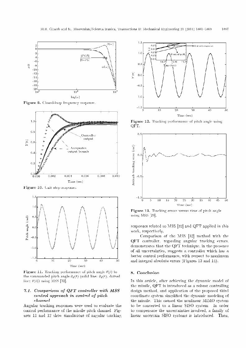
The frequency-domain closed-loop response isshown in Figure 9 and, consequently, the time-domainclosed-loop response is shown in Figure 10. Hence,according to linear simulation, the missile has ro-bust stability and can also satisfy tracking speci�ca-tions.


Figure 9. Closed-loop frequency response.

Figure 10. Unit step response.

Figure 11. Tracking performance of pitch angle �(t) tothe commanded pitch angle �d(t) (solid line: �d(t), dottedline: �(t)) using MSS [32].

7.1. Comparison of QFT controller with MSScontrol approach in control of pitchchannel

Angular tracking responses were used to evaluate thecontrol performance of the missile pitch channel. Fig-ures 11 and 12 show simulations of angular tracking

Figure 12. Tracking performance of pitch angle usingQFT.

Figure 13. Tracking errors versus time of pitch angleusing MSS [29].

responses related to MSS [32] and QFT applied in thiswork, respectively.

Comparison of the MSS [32] method with theQFT controller, regarding angular tracking errors,demonstrates that the QFT technique, in the presenceof all uncertainties, suggests a controller which has abetter control performance, with respect to maximumand integral absolute errors (Figures 13 and 14).

8. Conclusion

In this article, after achieving the dynamic model ofthe missile, QFT is introduced as a robust controllingdesign method, and application of the proposed thirdcoordinate system simpli�ed the dynamic modeling ofthe missile. This caused the nonlinear MIMO systemto be converted to a linear SISO system. In orderto compensate the uncertainties involved, a family oflinear uncertain SISO systems is introduced. Then,


Figure 14. Tracking errors versus time of pitch angleusing QFT.

an optimal robust PID controller for the linear processis designed. Finally, the results obtained from thecontroller output designed using the QFT method arecompared with reported results of a multiple slidingsurface controller designed by \Lu, Zhao. et al." [32]. Itis shown that the QFT technique suggests a controllerwith a better control performance.

Nomenclature

� Angle of attack (�)� Angle of sideslip (�)�p Small deviation of lift �n�d Small deviation of rotating �n�(S) Uncertain parameters vector!x; !y; !z Angular velocity components (rad/s)�� De ection angle in the pitch plane (�)�� De ection angle in the yaw plane (�)kd Derivative gain� Fractional derivative� Fractional integrationP (s; �) Uncertain plantXb; Yb; Zb Body coordinateG(s) CompensatorFx; Fy; Fz Components of total forces acting on

missile (N)Mx;My;Mz Components of total moments acting

on missile (N m)D(s) DisturbanceCx Drag coe�cientXg; Yg; Zg Ground coordinateki Integral gainu; v; w Velocity components (m/s)

S Laplace variableCz Lateral coe�cientCy Lift coe�cientIx; Iy; Iz Moment of inertia components (kg

m2/s)F (s) Pre-�lterkp Proportional gainr Reference signalM The mass of missile (kg)

References

1. Blacklock, J.H., Automatic Control of Aircraft andMissile, 2nd Ed., John Wiley & Sons Publition, NewYork, Chaps. 1, 4, 7, 8 (1991).

2. Zarchan, P. \Proportional navigation and weavingtargets", Journal of Guidance, Control and Dynamics,18(5), pp. 969-974 (1995).

3. Menona, P.K. and Ohlmeyer, E.J. \Integrated designof agile missile guidance and autopilot systems", Con-trol Engineering Practice Journal, 9(10), pp. 1095-1106 (2001).

4. Seraj, H. and Masominya, M.A. \Modeling and controlof a rotational missile", ICEE Conference, Isfahan, pp.10- 17, Printed in Farsi (2000).

5. Faruqi, F.A. and Lan Vu, T., Mathematical Models fora Missile Autopilot Design, 1st Ed., DSTO SystemsSciences Laboratory Publication, Edinburgh, SouthAustralia (2002).

6. Lidan, X., Ke'nan, Z., Wanchun, Ch. and Xingliang, Y.\Optimal control and output feedback considerationsfor missile with blended aero-�n and lateral impulsivethrust", Chinese Journal of Aeronautics, 23, pp. 401-408 (2010).

7. Ahmeda, W.M. and Quan, Q. \Robust hybrid controlfor ballistic missile longitudinal autopilot", ChineseJournal of Aeronautics, 24, pp. 777-788 (2011).

8. Mingzhe, H., Xiaoling, L. and Guangren, D. \Adaptiveblock dynamic surface control for integrated missileguidance and autopilot", Chinese Journal of Aeronau-tics, 26(3), pp. 741-750 (2013).

9. Gharib, M., Amiri Moghadam, A.A. and Moavenian,M. \Optimal controller design for two arm manipula-tors using quantitative feedback theory method", 24thInternational Symposium on Automation and Roboticsin Construction, India (2007).

10. Yaniv, O. \Automatic loop shaping of MIMO con-trollers satisfying sensitivity speci�cations", ASMEJournal of Dynamic Systems, Measurement, and Con-trol, 128, pp. 463-471 (2006).

11. Kim, C.S. and Lee, K.W. \Robust control of robotmanipulators using dynamic under parametric uncer-tainty", International Journal of Innovative Compen-sators Computing, Information and Control, 7(7(B)),pp. 4129-4139 (2011).


12. Bi, Sh., Deng, M. and Inoue, A. \Operator basedrobust stability and tracking performance of MIMOnonlinear systems", International Journal of Innova-tive Computing, Information and Control, 5(10(B)),pp. 3351-3358 (2009).

13. Tootoonchi, A.A., Gharib, M.R. and Farzaneh, Y. \Anew approach to control of robot", IEEE RAM, pp.649-654 (2008).

14. Fateh, M.M. \Robust control of electrical manipulatorsby joint acceleration", International Journal of Inno-vative Computing, Information and Control, 6(12), pp.5501-5511 (2010).

15. Moghadam, A., Gharib, M.R., Moavenian, M. andTorabi, K. \Modeling and control of a SCARA robotusing quantitative feedback theory", Proc. IMechEPart I: J. Systems and Control Engineering, 223(17),pp. 901-918 (2009).

16. Isidori, A., Nonlinear Control Systems, Berlin,Springer (1989).

17. Horowitz, I.M. \Survey of quantitative feedback the-ory", Int. J. Control Journal, 53(2), pp. 255- 261(1991).

18. Golubev, B. and Horowitz, I.M. \Plant rational trans-fer function approximation from input-output data",International Journal of Control, 36(4), pp. 711-723(1982).

19. Jayasuriya, S., Nwokah, O., Chait, Y. and Yaniv, O.\Quantitative feedback (QFT) design: Theory andapplications", American Control Conference TutorialWorkshop, Seattle, Washington (June 19-20, 1995).

20. Yaniv, O. and Horowitz, I.M. \Quantitative feedbacktheory for uncertain MIMO plants", InternationalJournal of Control, 43, pp. 401-421 (1986).

21. Kerr, M.L., Jayasuriya, S. and Asokanthan, S.F. \Ro-bust stability of sequential multi-input multi-outputquantitative feedback theory designs", ASME Journalof Dynamic Systems, Measurement, and Control, 127,pp. 250-256 (2005).

22. Zoloas, A.C. and Halikias, G.D. \Optimal design ofPID controllers using the QFT method", IEE Proc-Control Theory Appl, 146(6), pp. 585-589 (1999).

23. Lin, T.C., Kuo, M.J. and Hsu, C.H. \Robust adaptivetracking control of multivariable nonlinear systemsbased on interval type-2 fuzzy approach", Interna-tional Journal of Innovative Computing, Informationand Control, 6(3(A)), pp. 941-963 (2010).

24. Garc��a-Sanz, M., Ega~na, I. and Barreras, M. \De-sign of quantitative feedback theory non-diagonal con-trollers for use in uncertain multiple-input multiple-output systems", IEEE Proceedings-Control Theoryand Applications, 152(2), pp. 177-187 (2005).

25. Yang, S.H. \An improvement of QFT plant templategeneration for systems with a�nely dependent para-metric uncertainties", Journal of the Franklin Insti-tute, 346(7), pp. 663-675 (2009).

26. Wang, Y.F., Wang, D.H., Chai T.Y. and Zhang,Y.M. \Robust adaptive fuzzy tracking control with twoerrors of uncertain nonlinear systems", InternationalJournal of Innovative Computing, Information andControl, 6(12), pp. 5587-5597 (2010).

27. Zhang, Y., Liang, X., Yang, P., Chen, A. and Yuan,Z. \Modeling and control of nonlinear discrete-timesystems based on compound neural networks", ChineseJournal of Chemical Engineering, 17(3), pp. 454-459(2009).

28. Yanou, A., Deng, M. and I.A. \A design method ofextended generalized minimum variance control basedon state space approach by using a genetic algorithm",International Journal of Innovative Computing, Infor-mation and Control, 7(7(B)), pp. 4183-4195 (2011).

29. Chait, Y. and Hollot, C.V. \A comparison betweenH-in�nity methods and QFT for a SISO plant withboth parametric uncertainty and performance speci�-cations", O.D.I Nwokah, Ed., Recent Development inQuantitative Feedback Theory, pp. 33-40 (1990).

30. Horowitz, I.M. \Optimum loop transfer function insingle-loop minimum-phase feedback systems", Int. J.Control, 1, pp. 97-113 (1973).

31. Horowitz, I.M. and Sidi, M. \Optimum synthesis ofnon-minimum phase feedback systems with plant un-certainty", Int. J. Control, 27(3), pp. 361-384 (1978).

32. Lu, Zhao, Lin, Feng and Ying, Hao \Multiple slidingsurface control for systems in nonlinear block control-lable form", Cybernetics and Systems: An Interna-tional Journal, 36, pp. 513-526 (2005).

Biographies

Mohammad Reza Gharib was born in Mashhad,Iran, in 1981. He received BS and MS degreesin Mechanical Engineering, in 2004 and 2006, fromFerdowsi University of Mashhad, Iran, where he is cur-rently pursuing his PhD degree. His current researchinterests include control theories, mainly focusing onQuantitative Feedback Theory and the dynamics ofquadrotors.

Majid Moavenian received his Bachelor of Science inMechanical Engineering from the University of Tabriz,Iran. He also earned his MSc and PhD Degrees inMechanical Engineering from Aston University andUniversity of Wales College Cardi�, respectively. Cur-rently he is an associate professor at Ferdowsi Univer-sity of Mashhad while his research interests are in theareas of system design and fault detection.

Documents

Synthesis of robust PID controller for controlling a ...scientiairanica.sharif.edu/article_3580_65a77f92acd77c94e509f4bccd... · single input single output system using quantitative