SYNTAX AND SEMANTICS IN HIGHER-TYPE … · transactions of the american mathematical society Volume 276, Number I, March 1983 SYNTAX AND SEMANTICS IN HIGHER-TYPE RECURSION THEORY1

transactions of theamerican mathematical societyVolume 276, Number I, March 1983

SYNTAX AND SEMANTICS

IN HIGHER-TYPE RECURSION THEORY1

BY

DAVID P. KIERSTEAD

Abstract. Recursion in higher types was introduced by S. C. Kleene in 1959. Since

that time, it has come to be recognized as a natural and important generalization of

ordinary recursion theory. Unfortunately, the theory contains certain apparent

anomalies, which stem from the fact that higher type computations deal with the

intensions of their arguments, rather than the extensions. This causes the failure of

the substitution principle (that if <p(aJ+\ 31) and 0(ß', 91) are recursive, then there

should be a recursive «/(SI) such that <|/(Si) — <P(^ßj9(ßJ, 31), St) at least whenever

\ßj6(ßJ, 31) is total), and of the first recursion principle (that if F(f; 31) is a

recursive functional, then the minimal solution r of the equation F(f; 31) — f(3l)

should be recursive as well). In an effort to remove—or at least explain—these

anomalies, Kleene, in 1978, developed a system for computation in higher types

which was based entirely on the syntactic manipulation of formal expressions, called

y-expressions. As Kleene pointed out, no adequate semantics for these expressions

can be based on the classical (total) type structure Tp over N. In a paper to appear in

77ie Kleene Symposium (North-Holland), we showed that an appropriate semantics

could be based on the type structure Tp, which is obtained by adding a new object u

at level 0 and, at level (j + 1), allowing all monotone, partial functions from type y

into N. Over Tp, both of the principles mentioned above do hold. There is a natural

embedding to Tp into Tp.

In this paper, we complement the syntactic structure with a syntax-free definition

of recursion over Tp, and show that the two notions are equivalent. This system

admits an enumeration theorem, in spite of the fact that the presence of partial

objects complicates the coding of finite sequences. Indeed, it is not possible to code

all finite sequences from type j as type-y objects. We use the combination of the

syntactic and semantic systems to prove that, for any <p: Tp'-"'' -> N, the followingp

are equivalent:

A. <p is recursive in the sense of Kleene [1959],

B. <p is recursive in the sense of Kleene [1978], and

C. <p is the pull-back in Tp of some recursive ip: Tp(a) -» N.p

Using these equivalences, we give a necessary and sufficient condition on

9: Tp(o) -» N, under which the substitution principle mentioned above will hold forp

any recursive qp: 7p(T> -» N. With one trivial exception, the condition is that if y > 1,

then 31 must contain a variable of type greater thany. We feel that this result is

particularly natural in the current setting.

0. Introduction. The study of recursion in higher types was introduced by Kleene

[1959]. In this theory, rather than restricting one's attention to number-theoretic

Received by the editors March 16, 1981.

1980 Mathematics Subject Classification. Primary 03D65.

'This paper is a revised version of the author's doctoral dissertation at the University of Wisconsin,

Madison, 1979.

©1983 American Mathematical Society

0002-9947/82/0000-0328/$! 1.50

67

License or copyright restrictions may apply to redistribution; see http://www.ams.org/journal-terms-of-use

68 D. P. KIERSTEAD

functions, one considers functions taking their values in N (the natural numbers),

but whose arguments are taken from the collection Tp of objects of finite type over N.

Tp is defined recursively by

7><°> = N,

TpU+l~> = NTpU) = the set of total functions from Tpu) into N,

Tp = U Tpu\

One generally uses variables aj,ßj,..., to range over Tpu\ and 91,93,..., for

strings of such variables.

From the outset, this theory was recognized as a natural and important extension

of ordinary recursion theory. Unfortunately, two important principles fail in this

theory. The first is the substitution principle: If m(a", 9Í ) and 9(ß"~x, 91) are partial

recursive, then certainly X9I<p(\/3n~1ô(/3"~1, 91), 91) should be partial recursive.

Indeed, this principle seems so basic that its failure serves, at best, to dismay the

novice, and, at worst, to suggest that there may be something fundamentally amiss

with the theory. The second principle is the analogue of the First Recursion Theorem

of ordinary recursion theory: If F(f; 9Í) is a partial recursive functional, then the

minimal solution Ç of the equation F(f ; 9Í ) - f( 91 ) should also be partial recursive.

This second failure seems even more anomalous when one considers that the

analogue of the Second Recursion Theorem does hold.2

The problem underlying both of these failures is demonstrated by an example of

Kleene [1963, p. 110]. Here T(e, a, x) is Kleene's /"-predicate (see Kleene [1952, p.

281]).

0.1 Example (Kleene). Define

, JO if^T(e,e,x),

x(e'x'~ [undefined if Tie, e, x),

cp{o2,e) â2{Xxxie,x)),

0(a)-0,

«//(e) ^q>{\a0{a),e).

<p is partial recursive and <p(o2, e) is defined if and only if \/x-,T(e, e, x) (since

\xx(e, x) is total, hence a type-1 object, if and only if \/x-,T(e, e, x)). Were «//

partial recursive, then «// would be partial recursive in the sense of ordinary recursion

theory (Kleene [1959, XVII]). This is impossible since «//(e) is defined if and only if

Vx-,T(e, e, x), and the latter is not recursively enumerable. □

Perhaps one feels cheated by this example. One could easily argue that 6(a) is

defined without using any values of a(x), and therefore <p(\a0(a), e) should be

2Kleene [1959, 1963] did obtain restricted versions of both of these principles, but the basic anomalous

nature of their failures remained.


HIGHER-TYPE RECURSION THEORY 69

defined for all e. It is easy to construct more complicated 6 where it is not so clear

for what values of x the corresponding values of a(x) are used by 0 in determining

0(a); but there is still the feeling that if \xx(e, x) is (correctly) defined for all of

these x then <p(\a6(a), e) should be defined. Kleene seems to have shared these

misgivings and made a suggestion for remedying the situation (Kleene [1963, p.

111]). Kleene [1978] resurrected this idea. He argued that there was no need to

attempt a computation of xie> x) unul its value was called for in the course of

computing 0(\xx(e, x)). Thus we might simply carry x(e, x) along as a formal

expression until such a value is called for. Of course we might soon find ourselves

considering formal expressions within formal expressions ad nauseam, and it would

be no small task to keep all of the syntax straight. Having taken this approach,

Kleene was able to include analogues of the substitution and first recursion

principles as primitive operations and produce an emiently workable theory.

Kleene [1978] developed a system for computation in higher types which was

based entirely on the syntactic manipulation of formal expressions called "y-expres-

sions". Under a given assignment ß to the free variables of the language, each

O-expression is either undefined or defined with some natural number as its value;

each (j + l)-expression B naturally represents a partial function [B]a from T¿J) into

the natural numbers. [B]a need not be total, and thus need not be a type-(y + 1)

object. In the course of proving certain theorems in §3 of Kleene [1978], it was

necessary to know that oney-expression B could be substituted (freely) for another B

in a O-expression E without affecting the value of E under fi. Kleene [1978, p. 208]

used an example similar to Example 0.2 below to show that the condition [B]Q = [B]ü

is insufficient to justify these substitutions—even when [B]a is total. Kleene

postponed the justification of these substitutions pending the development of an

appropriate semantics for his system. The following example should be comprehensi-

ble, even to the reader unfamiliar with Kleene [1978].

0.2 Example. Let B be the 1-expression \a • cs(a, 0,0). (cs(a, b, c) — b if a — 0, c

if a > 0.) Let B be \a ■ 0. Clearly, for any assignment Q, [B]a = [B]ü. It is easy to

construct a O-expression A which is undefined under any assignment (see §3 of

Kleene [1978]). Let E be the 0-expression B(A). Then, under any ß, E is undefined,

but B(A) — 0. Thus B may not be substituted for B in E—even though [B]a = [B]a

for any il. The problem is that the "obvious" interpretation [B]ü of B does not take

into account whether B "uses" its argument or not. Although [B]a and [B]a are

extensionally the same, their intensions are different. D

These two examples indicate that an appropriate semantics for Kleene's system

must be based on a type structure somewhat different from Tp. In order to avoid

intentional considerations, we must allow a new object at level 0 which will

distinguish between the [B]a and [B]Q of Example 0.2. In order to avoid the

problem of Example 0.1, we must allow our functions to be defined even when their

arguments are incompletely defined. Finally, since we will only be computing values

of arguments when it is absolutely necessary, we must insure that the value of

aj+2(ßi+x) depends only on those values of ßJ+x(yJ) which are defined. That is,

aJ+1 must be monotone. In Kierstead [1980] we considered such an extension of the


70 D. P. KIERSTEAD

type structure and showed that an appropriate semantics for Kleene's 1978 system

could be based on this type structure in a natural way.3

We use the notations <p(9I)i and <p(9i) Î for "<p(9I) is defined" and "<p(9I) is

undefined" respectively.

0.3 The extended types. We define TpU) (the set of extended type-j objects,

henceforth denoted by typej) by recursion ony.

7><°>={u,0,l,2,...}=NU {u}.

(u is a new object suggesting " undefined".) Define a° C /3° <-> [a0 = u or a0 = ß0].

fpU+1) — (¿g set 0f au monotone, partial functions from Tp(j) into N.

tp = U fpu\y<co

(aj+x is monotone if, whenever aj+x(ßj)l and ßJ C yJ, then aJ+x(yJ)l and is equal

to aj+x(ßJ)—where " C " is the relation defined above at type Ô and has the usual,

set-theoretical meaning at all higher levels.) Let us write uj for the totally undefined

type-y object. Monotonicity requires (among other things) that if aJ+x(uJ) = w then

aJ+x =\ßj-w.* D

The computations of Kleene [1978] were based on a list of schemata (SO—SI 1).

These schemata were not to be thought of as actually defining functions, but merely

as rules to guide computations. While investigating the relationship between the

systems of Kleene [1978] and Kleene [1959], it became clear that it would be

convenient if SO-SI 1 actually did define functions in a natural way. This is the case

if one considers them as defining functions on Tp, rather than Tp. There is a natural

embedding # : Tp -* Tp of the classical type structure into the extended type

structure. This embedding extends to include partial functions on Tp. We will

describe # in §4.1. For the moment, it suffices to know that # exists.

In §1, we present the syntactic system of Kierstead [1980], which is obtained by

carrying out the computations of Kleene [1978] over Tp. In §2, we give a syntax-free

definition of the class of (partial) recursive functionals on Tp which directly mirrors

the syntactic system of §1. In §3, we compare these systems. In §4 we use the

combination of the syntax and the semantics to derive some results about the

original system of Kleene [1959]. §5 contains some additional properties of recursion

over Tp. §6 contains some general discussion of the relationship between this paper

and some other work in higher-type recursion theory.

Along the way, we will show that the following are equivalent for any partial

functions is partial recursive in 0 in the sense of Kleene [1978];

3 Kleene [1980, to appear] has developed a somewhat different semantics for his system.

4 That some semantics for Kleene's 1978 system was necessary, and that such a semantics would have to

be based on an extension of the type structure along the lines described above, were suggested by Kleene

[1978 and private communications]. Kleene [1980, to appear] has also pursued this idea and arrived at a

semantics significantly different from ours. Our type structure agrees with his at the 0 and 1 levels, but

differs from there on.



(iii) there is a «// (over Tp), partial recursive in #0 in the sense of this paper, such

that for all (a{\ ...,aJ„-)E TpUl) X •■■ X Tp(i»\

*(#<*,%..., #<»)=* <p(«í',...,<«).

In the preparation of this paper, we were strongly influenced by the ideas of

Kechris and Moschovakis [1977] and, of course, by Kleene [1959, 1963, 1978, and

1980].

The reader familiar with Platek [1966] will notice that our system is quite similar

to his—although we arrive at it from a very different direction. We will return to this

similarity in §6. For the moment, suffice it to say that we feel our system is

conceptually much simpler, and corresponds more closely to the actual process of

computation. It seems that the firm connection between the syntax and the semantics

of computations is an important aid to understanding a traditionally difficult

subject.

0.4 Notation and terminology. Our notion is, for the most part, standard in the

literature. All unexplained notation and terminology are from Kleene [1952 and

1959]. We use variables aJ, ßj, yJ,..., to range over Tp(J) or TpiJ\ depending on the

context. When it becomes necessary to make the distinction explicit we will use

àJ, ßJ, yj,..., to range over Tpu\ We may omit the superscript occasionally when

there is no danger of confusion—e.g., we may write aj(ß) or a(ßj~x) for aj(ßJ~x),

or \aJ0(a, 91) for Xajd(aJ, 91). We use 91,93, ©,..., for finite strings of such

variables. If 91 is (a{\...,a{") and 93 is (ß{\... ,ßi"), we write 91 C 95 to mean that

a{1 C ß{',.. ,,aJn" C ßj". lía = (y,,... ,j„) is a finite sequence from N, we write Tp(a)

for TpUi) X ■ ■ ■ X Tpu"\ and similarly for Tp(a). We say that the character of 9t is a

(ch(9i) = a) if 91 ranges over Tp(a) or Tp(a). By maxtp(9I), we mean the maximum

type of any variable in 91. Similarly, if ch( 91 ) = a, then max tp( a ) = max tp( 91 ). We

use a, b, c,..., as variables whose intended range is N, but do not exclude the

possibility that a — u E Tp(0\ 0 will always stand for a list (6X,.. .,6,) of function

variables whose arguments are from various (specified) 7/>(o) or Tp^. We have the

usual meanings for = , ¥^ , — , ^ . In particular, <p( 91 ) ¥" «//( Ê ) means that both

are defined and with different values, while <p(9i) ¥ «//(93) means that it is not the

case that <p(9t) ̂ «//( 93 ).5

Function will always mean: monotone, partial function taking values in N.

("Monotone" is superfluous when working over Tp.) We shall frequently abuse

notation slightly by writing: <p(9I) C «//(93) to mean [<f>(91) Î or <p(91 )-«//(93)],

<p(9l) =* a0 to mean [<p(9t) | and a0 — u, or <p(9t)| and <p(9t) = a0], etc. (This is an

abuse of notation since (¡p(9I) has no value if <p(9I) î .) By X-* Y(X -» Y) we mean

the collection of monotone, partial (total) functions from X into Y. As usual, we

write <jp : X -» Y to mean q> E X ^>Y.p p

We will also be dealing with monotone (partial) functionals (henceforth referred

to as functionals) q>(0x,.. .,$,; 91), where each 0, ranges over some 7/7(0,)-»N (or

5Thus, qp(9I) ¥=ip(m) is not the same as -,(<p(3I) = «//(SB)).


72 D. P. KIERSTEAD

7yo.) _» ¡vT) an(j gt ranges over some 7¡r7(o) (or fpia)). By monotone we mean that <p isp

monotone both in its function arguments and in its object arguments. That is to say:

If 0X C f),,... ,0, C 0, and 91 C 9Î then <p(0; 91) C m(0; 9t). We do not exclude the

possibility that / = 0 (so <p is a function) or that 91 is empty.

We write dom(tp) for the domain of <p.

We use arbitrary Greek letters for ordinals. We trust that the reader will forgive us

and sympathize with us for having run out of alphabets. In any event, there should

be no cause for confusion.

1. The syntactic system. We describe briefly the schemata S0-S11, and the

definition of j-expression, from Kleene [1978]. The reader desiring more details is

referred to that paper.

1.1 7716° schemata. For the moment, the following schemata should be viewed as

merely formal expressions. In particular, one should not worry about the " meaning"

of S4.y or SI 1. (The numbering comes from Kleene [1978] and is designed to

correspond, where possible, to that of S0-S9 from Kleene [1959].) In S6.y, 91 is the

sequence which results from 91, by moving the (A: + l)st type-y variable to the front

of the list (so it should really be called S6.y, k). We will explain the schemata more

fully below:

(SO) <p(0; 93, S) -0,(93).

(S1.0) m(0;a,93)-a-r- 1.

(SU) <p(e;a,V)â-ll^(a0-1 j£>£

(S2.0) m(0;9i)-O.

(S3) m(0;a,93)-a.

(54.0) q,(0; 91)-«//(©; x(0; 91), 91).

(S4.y) (y > 1) m(0; 91) - «//(©; Xß^xiî ßJ~\ 9í), 9í).

(55.1) <p(0; a, b,c, 93) - cs{a, b, c) = { * jj¡¡ > J

(S6.y)(y3*0) <p(0; 9t) - ^(0; 9Í,).

(S7.y) ij> 1) <p(0; «>,«>"', 93) - «V')-(Sil) (p(0; 91) - «//(A9T(p(0; 91'), 0; 9Í). [=* «//(<p, 0; 9Í) briefly].

The schemata are to be applied under the convention (adopted in Kleene [1959, p.

3]) that only the order of the variables within each type is significant,

While S0-S11 do not actually define functionals by themselves, we will often

speak of them as though they did. The «// and x on the right sides of some of the

schemata are to be symbols for functionals previously generated via S0-S11. In SI 1,

«// must have one more function argument than does <p, and this argument must range

over fp(a) ^N, where ch(9l) = a.p

A derivation of (p (via SO-SI 1) is a sequence <p,,... ,x — <p, , via one of S0-S11, (ii) each <¡p, except cpp



is used as a «// or a x in a later application of one of S0-S11, and (iii) if <p. follows

from «// (or «// and x) via one of S0-S11, then <p,,...,<p, is «//,,.. .,\pr, <p, (or

"rV-••>>/',-, Xi»---»X?» <P,), where «/-,,.. .,«//r and Xi.-»Xfl are derivations of «// and x

respectively. (Kleene called these "canonical derivations", but we will never consider

any other kind, so we drop the adjective.)

It should be noticed that: If <p,,... ,<pp = <p in a derivation of <p(0; 91), then each

tp, is of the form ^(tT,, 0; 93) for some (possibly empty) list if, of function variables.

This is because the list of function variables only changes at applications of SI 1,

where the first function variable is phased out. Thus, if <p, is <p,(tj,, t/2, t/3, 0; 93), we

have a notion of r\2 having been phased out by identification with A©<pA(7}3, 0; K)

(here h > i). Of course, t)3 will also be phased out by some \d(pk(@; i?) with k> h.

Clearly one may devise an indexing scheme to code up every detail of a given

derivation (including the number and type of each of the variables of each <p,). We

are trying to avoid such details, so we suppose that this has been done in some

reasonable manner.

1.2 The j-expressions. We will work with a formal language, the terms of which are

called j-expressions. We write A = B to mean that A and B are the same formal

expression. The language is given relative to a fixed list 0 = (0,,.. .,0,) of (typed)

"assumed function" symbols.

The language consists of:

(i) the function symbols 0,

(ii) for each a E u<a, the function symbols <p°^°, ç>2^°> • • • >

(iii) for each y > 0, the object variables y¿, y{,... (using aj, ßj, etc. as "metavari-

ables" to represent arbitrary formal variables),

(iv) the symbols X, +1, — 1,0, and cs,

(v) commas, parentheses, and braces. D

The class of j-expressions is defined inductively by the clauses:

El. A type-y variable y/ is ay-expression.

E2. If Ax,... ,An are, respectively, y',-,... ,yn-expressions and a = (jx,...,j„), then

for each i, <p°"° (Ax,... ,An) is a O-expression. (The tp,'s will correspond to the <p¿'s of

some particular derivation.)

E3. If A is a O-expression, then \ajA is a (j + l)-expression.

E4. If A is a (y + l)-expression and B is ay-expression, then {^4} (B) (often

abbreviated A(B)) is a O-expression.

E5. 0 is a O-expression.

E6. If A, B,C are 0-expressions, then so are (A) + I, (A) — I and cs(A, B, C).

El.lfAi,...,A„ are, respectively, y',-,... ,y„-expressions and 0, ranges over

fpu.■'"»^N,p

then 0l(Ax,... ,An) is a O-expression. D

Computations will always be conducted with some fixed derivation q>,,...,<p in

mind, and the derivation will determine completely the a for the formal symbol

(jpf^0. Therefore we may safely drop the annoying superscript. We have ignored the

list of function arguments in the E2 clause because 0 remains fixed throughout, and


74 D. P. KIERSTEAD

any additional function arguments r¡ (as in (p¡(r¡, 0; 91)) are associated with the

unique function symbols <pk which phase them out in the given derivation—as will

become clear.

1.3 Computations. We now take ß to be an assignment of objects from Tp to the

object variables of the language, and of monotone, partial functions on these objects

to the function symbols 0. E will always represent a O-expression. We will only

compute values of O-expressions (although this will yield a notion of "value" [B]a

for ay-expression B). We give an inductive definition of [E]a = w (E has value

w E N under ß). Formally, we define K — {(E, ß, w): [E]a = w} by stages K*,

indexed by ordinals, taking K = UiÄ'i. In §1.4 we will show how this may be

viewed as a computation procedure. We will use the following notations:

ß[yVxy] is tne assignment obtained from ß by assigning xj to yJ,

JT« = U Ks,

«<f

[aJ]a — the object (in fpu)) assigned to aj by ß,

[0,]a = the function assigned to 0, by ß,

[ u if there is no such w,

and, for any (j + l)-expression B,

[B]? = XxiBiyJ)]%yJ/xJ]

(so [B]^ is a partial function from fp(j) into N). ([B]^ is the part of [B]a built up

before stage £.) Note: we really do mean to use " = " (not " — ") in the definition of

[E]qK Thus [E]q* may be u; but in the definition of [B]^, we are really defining a

function—so its values are restricted to N, with [B]q((xj) undefined if

Wï'M&vx/] = u.We will need to know that [B]q( E fp(J+X), i.e., that it is monotone, so we prove

the following lemma simultaneously with the definition of K.

1.3.1. Lemma. If, for each free variable aj ofE, [aj]ü C [aj]Q„ then [E]^( C [£]„!

In particular, [B]^ is monotone.

The definition of (E, ß, w) E K* is by cases, according to the form of £ as a

O-expression. The E4 case splits into two subcases according to the form of the "A "

in {A} (B) as a (y + l)-expression. In each case the lemma follows easily from the

inductive hypothesis.

1.3.2. Definition. In each of the nine cases, we specify the condition which must

be met in order to have (E, ß, w) E KK

El. E is a0 and [a°]a = w.

E2. E is tp¡iA{*,... ,A{") and (E*, ß, w) E K^, where E* is the result of making

the same substitutions (with proper attention to bound variables) on the right side of

the schema introducing <p,. as yields E on the left side. One point deserves some

clarification: If tp, is introduced via SO with the "0," actually an tj to be phased out



later via SI 1, say <p,(tj, 0; 91) - tj(91) and <pk phases out r; by <pk(@; 91) -

<p„(<pk, 0; 91), then E* is to be <pk(A), not i\(A).

E4.X. E is {XaU} (B) and (S$A | , ß, w) E K^. (S%JA | is the result of substitut-

ing B for each free occurrence of aJ in A, after changing bound variables ap-

propriately.)

E4.y. E is aJ(B) and aJ(ßJ~x) = w, where a¡ = [aJ]a and /3^~' = [B]^(. (Note

that the inductive hypothesis assures us that ßj~x E fpu~X).)

E5. £ is 0 and w — 0.

E6 + . E is A + 1 and (j4, ß, w0> E K<(, where w = w0 + 1.

E6 — . E is ,4 — 1 and (A, ß, w0) E K<i, where w = w0 — 1.

E6c5. E is cs(./4, 2?, C) and either:

(i) (A, ß, 0> E #<* and <5, ß, w) E K^, or

(Ü) (A, ß, 77 + 1> E tV<î for some 77, and (C, ß, w> E K<è.

El. E is 0,(—) and the condition similar to that of E4.y holds.

This completes the definition of K. □

1.3.3. Definition. Let B be ay-expression and E a O-expression.

(i) [B]a = Uî?]^. (This agrees with the previous definition for the case

B = a>.)

(ü)

.c-1 [the least £ such that (E, Q,w)E Ki for some w if such a ¿exists,I In 1

[ 00 otherwise. □

We will generally use induction on \E\a in situations where Kleene (in Kleene

[1978]) used "induction on computation trees."

1.4 Computation trees. For each E, ß, we describe the construction of a computa-

tion tree based on E, ß. If [E]ü I the tree will be well founded (in the sense that all

paths are finite) and the base node will have rank \E\Q. Each completed tree will

have a value associated with it and this value will be [E]Q. These trees are essentially

the same as those in §2.4 of Kleene [1978], except that we must alter the El, E4.y

and E7 steps (which correspond to the evaluation of a variable) to account for the

fact that we are dealing with a different set of objects. We picture our trees as lying

on their sides and growing from left to right. The principal branch issuing from a

vertex is the branch proceeding horizontally to the right. When a tree is completed,

we will tag the principal branch with the value of the tree. (In order to make our

claim about the rank of the tree hold, we must not consider the tag to be a part of

the tree.) Each vertex of the tree is occupied by a O-expression. With each vertex,

there is associated an assignment in force at that vertex.

Consider a vertex occupied by E with ß as the assignment in force. By cases on E,

we describe the next level of growth beyond this vertex.

El. E is a0. If [a°]a = u there is no growth and the tree cannot be completed. If

[a°]a = w E N then the tree is completed by tagging it with the value w.

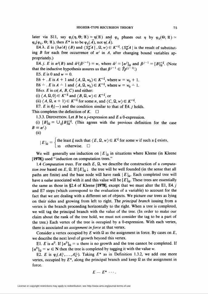
E2. E is cp¡(AJx',.. .,AJn"). Taking E* as in Definition 1.3.2, we add one more

vertex, occupied by E*, along the principal branch and keep ß as the assignment in

force.

E — E* ■■■ .


76 D. P. KIERSTEAD

E4.X. E is {XaJA}(B). We add one more vertex, occupied by S%JA | , with ß the

assignment in force.

{\aJA}(B)-S£A\---.

EA.l. E is ax(B). Take â1 = [al]0.

Case 1. â'(u)|. The tree is completed by tagging it with the value â'(u).

Case 2. Otherwise. We place B (under ß) at the lower, next vertex and begin a

computation tree for B. If this tree is completed at some stage with value w and

âx(w)l, then the tree for E is completed by tagging it with àx(w).

ax(B)-âx(w)

~~~^~~~-B ■ ■ ■ w

Otherwise, the tree for E cannot be completed.

E4.y (y > 1). E is a>(5). Take A* = [a%.

Case 1. âj(uJ~x)l. The tree is completed by tagging it with the value «•'(u-'-1).

Case 2. Otherwise. We begin simultaneous computations of B(yj~2) (for some

new variable yj~2) under each assignment ß[y-/'_2/X7'-2] f°r XJ~2 e Tpj~2. As

these computations proceed, one step at a time, some of them may become

completed with values wxj-i E N. As computations become completed, we add them,

at lower, next vertices, to the computation tree for a\B). In this way, we build up in

i steps, partial functions ß(~x: Tpu~2) -*N by taking

/TV"2)-

WxJ-s if the computation of

B(yj~2) under Q[yJ~2/xJ~2]

was completed in < £ steps,

undefined otherwise.

Notice that ß[ is just [B]^. When and if at some stage £, we have aJ(ß{ x){, the

tree for aJ(B) is tagged with this value.

aJ(B)— —aJ(ßi~x)

B{yJ-2)---Q[yj-2/xi'2] w„

B{y

B(y~2)-

ß[7;"Vxi"2]

®[yJ~2/xi-2]

Xi

E5. E is 0. The tree is tagged with 0.

E6 + . E is A + I. We place A at a lower, next vertex and begin computing A

under ß. When and if this computation is completed, say with value tv, the tree for

A + I is tagged with w + 1.

A + 1^—-w + 1

^^~~~^^l ■ ■ ■ w



E6 — . E is A — 1. Similarly.

A-I.

E6 cs. E is cs(A, B, C). We compute A (under ß) at a lower, next vertex. When

and if this computation is completed, we place either B or C at the next vertex along

the principal branch from E, according as the value for A was 0 or > 0.

B ■■■ ifw = 0,

<*(A>B>C^ ifw>0,

• • w.

E7. E is 6,(A{', ...,AJn-). Similarly to E4.y, we build up partial functions â{\ ...,âJn-

until we have sufficiently large arguments for [0,]n(â{\.. .,âJn") to be defined, at

which point we tag the tree for E.

This completes the procedure for constructing computation trees. We shall seldom

make actual use of the trees, but they serve well to guide the intuition. If

(E, ß, w)E K( then the next vertices after E include all those expressions whose

values were required in the determination that (E, ß, w)E K(. The entire tree

contains precisely the information that was " used" in determining that (E, ß, w) E

K.

1.5 Discussion. In this section, we attempt to justify aspects of our computations

which may appear to violate the spirit of computability.

At the E4.y step, we are, in general, obliged to attempt computations of B(yj~2)

(under assignments ß[yJ_2/xJ 2]) which cannot be completed. This is a significant

deviation from the traditional approach, where a single uncompletable subcomputa-

tion will frustrate the entire computation. The next example will show that, under

any reasonable semantics for Kleene's formal system, such computations will have to

be begun.

If, at step E4.y, we are only allowed to begin computations of B(yJ~2) under

ß* = ß[y^"2/xJ'"2]forvaluesofxj'"2suchthat[73(y^-2)]na,andif[a>]ß(uj'-1) î ,

there will have to be a xJ~2 such that

vßJ-x{[«JUßj-x)^ßj-\xJ-2)i).

This is because the assignment to yy~2 for the first subcomputation would have to be

chosen with no a priori knowledge of [B]a, and will have to be in the domain of

[B]a.If every y'-expression is to represent an object in 7¡p(7), and if semantically

equivalent y'-expressions are to yield the same value when substituted (freely) in any

0-expression, then the same will have to hold with anyy-expression A in place of aJ.

That is, given A, ß with [ A]a(uJ ~ ' ) Î , there must be a xJ ~2 such that

W-yiAMßJ-î-ßJ-w-î)-We now present an example of a 3-expression A for which no such x may be

chosen.6 There are simpler examples, but they make use of specific derivations

6 This situation does not occur at types 0, 1, or 2.


7 S D. P. KIERSTEAD

(including SU). This example shows that the situation is basic to the definition of a

y-expression and independent of the specific schemata allowed.

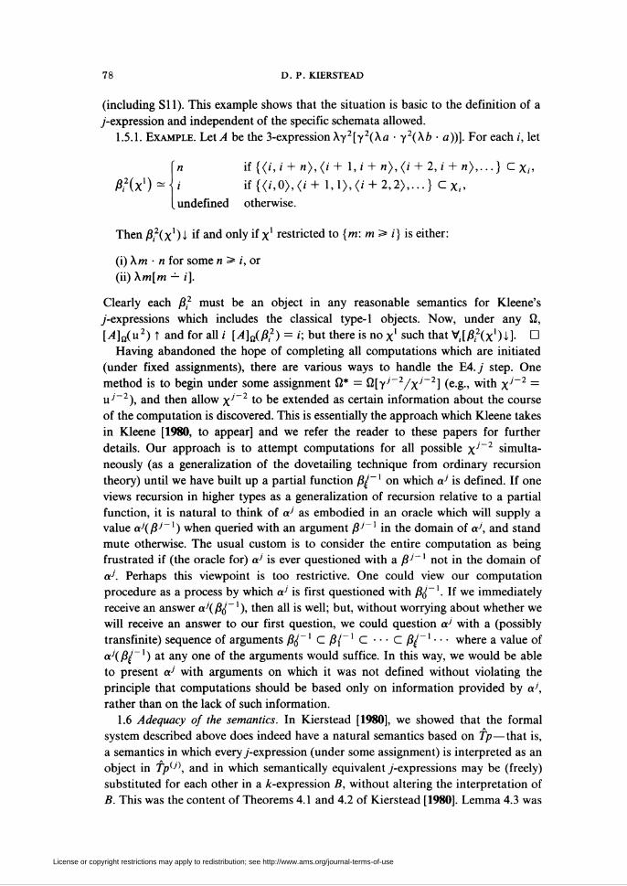
1.5.1. Example. Let A be the 3-expression Xy2[y2(Xa • y 2(Xb ■ a))]. For each i, let

Aa(x')n if {</,/+ /7>, (/+ l,i + n),(i + 2,i + n),...} C X/>

i if{</,0>,(z+l,l>,<7 + 2,2>,...) CX„


Then /32(x')l if and only if x1 restricted to {777: m > 1} is either:

(i) Xm • n for some 77 > i, or

(ii) Xm[m — /].

Clearly each ßf must be an object in any reasonable semantics for Kleene's

y'-expressions which includes the classical type-1 objects. Now, under any ß,

[A]a(u2) î and for all i [A]a(ß2) = i; but there is no x1 such that V,[/3,2(x')i]. □

Having abandoned the hope of completing all computations which are initiated

(under fixed assignments), there are various ways to handle the E4.y step. One

method is to begin under some assignment ß* = ß[Yy~2/xy~2] (e.g., with xJ~2 =

uJ~2), and then allow x'1 to be extended as certain information about the course

of the computation is discovered. This is essentially the approach which Kleene takes

in Kleene [1980, to appear] and we refer the reader to these papers for further

details. Our approach is to attempt computations for all possible xj2 simulta-

neously (as a generalization of the dovetailing technique from ordinary recursion

theory) until we have built up a partial function ß£~ ' on which aJ is defined. If one

views recursion in higher types as a generalization of recursion relative to a partial

function, it is natural to think of aJ as embodied in an oracle which will supply a

value aJ(ßJ~x) when queried with an argument /3y_1 in the domain of aJ, and stand

mute otherwise. The usual custom is to consider the entire computation as being

frustrated if (the oracle for) aj is ever questioned with a ßJ~x not in the domain of

aJ. Perhaps this viewpoint is too restrictive. One could view our computation

procedure as a process by which aJ is first questioned with ß£~x. If we immediately

receive an answer aj(ß&~x), then all is well; but, without worrying about whether we

will receive an answer to our first question, we could question aJ with a (possibly

transfinite) sequence of arguments /3¿_1 C ß{~x C • • • C ß£~x ■ ■ ■ where a value of

aj(ß£~x) at any one of the arguments would suffice. In this way, we would be able

to present aj with arguments on which it was not defined without violating the

principle that computations should be based only on information provided by aJ,

rather than on the lack of such information.

1.6 Adequacy of the semantics. In Kierstead [1980], we showed that the formal

system described above does indeed have a natural semantics based on Tp—that is,

a semantics in which every y-expression (under some assignment) is interpreted as an

object in Tp(J\ and in which semantically equivalent y-expressions may be (freely)

substituted for each other in a ^-expression B, without altering the interpretation of

B. This was the content of Theorems 4.1 and 4.2 of Kierstead [1980]. Lemma 4.3 was



a technical lemma which proves to be useful. We restate these here as 1.6.1, 1.6.2,

and 1.6.3 respectively.7

1.6.1. Theorem. Let B be aj-expression. Then [B]a E fpU). D

1.6.2. Theorem. Let E be a O-expression. Let D, D be j-expressions not containing

the variable ßj. Let ED = SÊ \,E^ = S$E \ . Then, for any ß

[D]a{Ç}[D]a-*[Ej>]u{Q}[EE]a. D

1.6.3. Lemma. Let B be aj-expression and A a (j + l)-expression, where neither A

nor B contains the variable yJ. Suppose [A(B)]a 1, say \ A(B) \a = £. Then

[A(B)]Q=[A(yJ)]ü[yJ/{Brat]

and

\AiB)\Q>\AiyJ)\QlyJ/m<(]. O

Finally, we obtain the notion of a (partial) recursive functional over Tp by

considering a fixed derivation <p,,...,<p = tp, and associating with the O-expression

<p(9I) the functional

Xr¡, 93[<p(9í)]o,[e/í;5[/a9]-

In Kierstead [1980] we showed that, when this notion is pulled back to Tp (via the

embedding #), the theory of Kleene [1978] is obtained. We shall return to this in §4.

2. The syntax-free system. In this section, we develop a syntax-free character-

ization of the class of recursive functionals over Tp. As in other such systems (e.g.,

Platek [1966], and Kechris and Moschovakis [1977]), the basic operation is the

process of taking the least fixed point of a given functional.

2.1 Fixed points. Following Kechris and Moschovakis [1977], we call a (monotone,

partial) functional <jp(tj, 0; 91 ) operative if -q ranges over Tp(a) -* N, where a = ch(91 )p

(i.e., if 7)(9t) makes sense). If cp(rj, 0; 91) is operative, we may define a monotone

partial functional tp°°(0; 2t), by recursion on ordinals |, via the equations:

<?*(©; 9!) ̂ <p( U X9lV(0;9i'),0;9l),

(p°°(0; 9Í) = w «(3^)^(0; 91) = w.

For convenience, we write

<p<í = U «p».

We write

\çx. w \ Ítrie least £ such that ^(0; 91 ) i if such exists,

^ L oo otherwise.

Actually, 1.6.3 is a special case of Lemma 4.3. Lemma 4.3 was stated in a rather complicated manner in

order to provide a sufficiently strong inductive hypothesis.


80 D. P. KIERSTEAD

When there is no danger of confusion, we may write | 0; 9Í \v as | 9Í |^, or | 0; 911 , or

even | 911 .

It is trivial to show (by induction on £) that these equations do indeed define a

monotone partial functional tp00. By a simple cardinality argument, there is a £ such

that

(Vfi>|)<p8 = <p* = <p°°.

We call tp00 the least fixed point of <p (as is justified by the following lemma).

2.1.1. Lemma. Let <p(tj, 0; 91) be operative. Then:

(i) (V9I, 0)[<p(X9ty°(0; 91'), 0; 9t) * <p«=(0; 91)].

(ii) (V0) ifé; fp^ ^N satisfies X9l<p(.//, 0; 9Í) C «//, then X9I<p°°(0; 9Í) C «//.p

Proof, (i) is immediate from the fact that <p°° = m* = <pi+1 for some £. (ii) follows

by an easy induction on £, using the monotonicity of <p (i.e., one proves that

V£[X9iy(0; 91) C «//]). D

2.2 TTie recursive functional. We use S0-S7 exactly as they are written in §1.1; but

as we are now viewing them as actually defining functionals (in §1 and Kleene

[1978], they were merely rules for computation), we refer to them as S'O-S'7. The

only schema which is different is ST 1, which we state as:

STl.<p(0;9I)-='/'''o(0;9t).

We will show in §3 that S0-S11 are really the same as S'0-ST 1. After that, we will

drop the distinction.

Since we are now defining functionals, we must say something about the meanings

of the various schemata. In ST.O, S'l.l, and S'3, 0 and c = u; however, <p will be defined if say

a— X, c — I, and b = u. Thus cs(a, b, c) is "strong definition by cases".8 In order

for S'4 and ST 1 to make sense, we must known that the x and «// on the right sides of

these schemata are monotone. It follows by an easy induction that only monotone

functionals may be obtained via S'0-STI. Notice that, since we are working over

Tp, there is no problem if XßJ~'x(0; ßj~x, 91) in S'4.y is incompletely defined. If,

inS'4.O,x(0; 2t) Î , then <p(0;9i) is to be .//(©; u, 31).

We call tp(0; 91) recursive if <p is definable via S'0-ST 1. (p(r¡; 91) is recursive in 0

if there is a recursive «// such that (Vrf, 9í)[(p(7f; 9Í) = «//(if, 0; 91)]. Recursive func-

tionals need not be total.

As in §1.1, we have the notion of a (canonical) derivation of <p.

An operator D: Tp(a) -> Tpu+X) is recursive (in 0) if there is a recursive (in 0)

function tp: fp(J) X fp(a) ->N such that, for all 9Í E fp(a),

I>(91) = XßJ<p(ßJ,%).

There seems to be some question in the literature as to whether this should be called "strong" or

"weak". We are using the word as established by Kleene [1952, p. 337].



Notice that a recursive operator is monotone, in the sense that

9Í C «'=>/>(31) C£>(9T).

The value of a recursive operator at some list of arguments may be substituted for an

object variable via S'4. y + 1.

Since we allow unlimited use of S'4, it is entirely possible that a given derivation

of say <p(a°, /?', y2) involves functions of say type-4 variables. We will see in §5 that

this need not be the case, i.e., if max 7/7(91) < r > 0 and each of 0 has only

arguments of types < r — 1, then <p(0; 91) has a derivation in which S4.y is only

used withy < r — 1.

The class of recursive functionals has several obvious closure properties which we

shall use in the sequel without comment. Among these are: permutation and

addition of variables of both sorts, definition by cases, identification of variables

(i.e., if \p(aJ, ßJ, 93) is recursive, then so is q>(aj, 93) - \p(aJ, aJ, 93)), and explicit

definition using +1, — 1, cs and the X operator. The proofs of all these are routine.

The details may be found in Kleene [1978]. (His proofs were carried out in a

different system, but they remain formally the same in the present context.) As an

example, we prove the functional substitution lemma. It should be noted that this

lemma was not so easy in the system of Kechris and Moschovakis [1977]. This is

because they did not allow iterations of STL

2.2.1. Lemma (Functional substitution). Let

<p(Px,...,P„,®;%), xA9;%i, »),.-• ,X„(e;3ía,93)

be recursive. Then so is «// where

«//(©; 93) -<p(A9i, • x,(0; 91,, 93),...,X9I„ • x„(0; 9I„, 93), 0; 93).

Proof. For notational convenience, we write X91x(0; 91, 93) for

X9ilXl(0;Si1,93),...,X9I„xn(©;9I„,93).

We first prove the more general statement, that there is a recursive 4> such that

>¿ (0; 93, 93*) ̂ <p(X9Ix(0; 91, 93*),0; 93).

The proof is by induction on the length of a given derivation of <p. Throughout the

induction, ch(93*) must, of course, remain fixed, but ch(93) will be determined by

the function to which the inductive hypothesis is to be applied. Thus, for example, if

<p was introduced by S4.0 as

<p{p,Q; 93) - (po(p,0; tp,(p,0; 93), 93)

we would assume the existence of a \p0 such that

«¿o(0; a, 93, 93*) =* <po(X9lx(0; 9Í, 93*), 0; a, 93).

We take cases according to the schema used to introduce «p. The only nontrivial case

is STL

Suppose <p was introduced by

<p(p,0; 93H <p-(p,0; 93)


82 D. P. KIERSTEAD

(so <p0 is <p0(tj, p, 0; 93)). By the inductive hypothesis (and the simple closure

properties mentioned above), we may find a recursive, operative «//0 such that

«¿oa, 0; 93, 93*) - <p0(X93' ■ f(93', 93*), X9Í ■ x(0; 91, 93*), 0; 93).

We show, by induction on £, that (for all 0, 93, 93*)

$(0; 93, 93*) - ró(A9íx(0; 91, 93*), 0; 93).

By simple calculation,

$(0; 93, 93*) - «¿0(X93'93*' • ̂ «(0; 93', 93*'), 0; 93, %*)

« (po(X93'^(0; »'. »*), *2tx(<=>; 91, 93*), 0; 93)

- «p^'tp^Xä • x(0; 31, 93*), 0; 93'), X9Í • x(0; 91, 93*), 0; 93)

(by the ind. hyp.)

-<pí(A9l-x(0;9í,93*),0;93),

as desired. In particular,

«/¿°(0; 93, 93*) - <p%(X9I • x(0; 9Í, 93*), 0; 93).

Thus, we may take «// = «//J0.

Finally, we use identification of variables to obtain

,//(©; 23)^(0; 93, 93) ̂ <p(X9i • x(3I, »),e; »). □

2.2.2. Lemma (Primitive recursion). // «// and x are recursive, then so is the

functional (®;a + l,93)-x(0;ö,<p(0;a,5B),93),

<p(0;u,93)î .

(Note. We are working over Tp, so it is entirely possible that <p(0; a, 93) Î and

<p(0; a + 1, 93H —as is the case ifxi®; a, u, 93)4 and «//(0; 93) Î .)

Proof. Define (using cs(—, —, — ))

>K0;93) ifa = 0,<Po(t},0;í7, 93)

' x(0; a - 1,77(0 - 1, 93), 93) ifa>0.

It is easy to check, by induction on a, that <p0(Xa'93' • <Pq(@; a', 93'), 0; a, 93) =*

<p(0; a, 93). Thus, by Lemma 2.1.1, tp^(0; a, 93) « tp(0; fl> 23). D

By

«4^(0; x, at) *o],

we mean: the least x E N such that «//(©; 0, 9t),... ,«//(©; x, 91) are all defined and

«//(©; x, 9Í) = 0, if such an x exists—otherwise px[\p(@; x, 9t) =* 0] is undefined.

2.2.3. Lemma (Least-number operator). //«// « recursive, then so is

<p(0; 91) =ujc[^(0;x, 9Í) =0].



Proof. Define

\x if«//(0;x, 9Í) = 0,

It is easy to check that

X°°(0; x, 91) - py[y > x and «//(©; v, 91) - 0].

Thus

Xoo(0;O,9I)-ux[^(0;x, 9t)-0]. D

2.2.4. Lemma. // <p: Tp®'0, •,0) ->N is partial recursive in the sense of ordinary

recursion theory, then <p is recursive in the present sense ( when tp is viewed as a function

on Tp(0'- ,0) whose domain happens to be a subset of Tp(0' ,0)).

Proof. In view of the preceding lemmas, the proof is a trivial induction on the

definition of (p. The only problem is that we must make sure that, if any of 93 is u,

then <p(93) î . This is easily handled using cs( —,—,—). For instance, if we set

«/-0(x, y) - cs(x, «//(*, y), «//(*, y)),

«//,(*, y) « cs(y, xp0ix, y), «//0(x, y)),

then

[undefined otherwise. D

3. The connection between syntax and semantics. In this section, we show that the

recursive functionals on Tp are precisely those obtained via the computations of §1,

and that the same functional is produced by a given derivation—whether via

SO-SllorS'0-STl.

Consider a derivation <p,,...,<p via SO—SI 1. By the corresponding derivation via

S'0-STI, we mean the derivation \px,...,\pp where «//, is introduced via S'0-STI in

exactly the same way that tp, was introduced via SO-SI 1. For example, if

(Sil) <p,(0;9í)-(p,._,(<p„0;9í)

then

(S'il) «//,(©; 91)-^,(0; 91).

Of course, we require that the variables of \p¡ be of the same number and types as

those of <p,.

3.1. Theorem. Let <px,... ,<pp be a derivation ofcp = <pp via S0-S11. Let «//,,... ,\pp =

«// be the corresponding derivation via S'0-S' 11. 77¡e7z, for all 0 and 91,

,//(©; 91)-<p(0; 91),

in the sense that for all assignments ß

<M[0]ß;[3i]ö)-k(2i)]o,( Recall that 0-expressions never show 0 explicitly.)


84 D. P. KIERSTEAD

Proof. The lists of function arguments of the various <p, (and «//,) will vary with t,

but will always be of the form (tj/+1,. .. ,tj„, 0), where 77 is the number of applica-

tions of Sll (see §1.1). For notational convenience, we will write (j\„ ©) to mean

(n(+1,...,T}„,0) where <p, has n — i function arguments in addition to 0. In

particular, ï\p is an empty list. We should really write 91, as well, since the list of

object variables changes also; but it is not quite as important to keep track of these,

so we avoid the additional subscript.

Let ß be an assignment. We will generally use the same symbols, 0 and 9Í, for the

formal variables 0 and 91, and for the functions [0]ß and objects [9t]n assigned to

them by ß. However, we must be careful to distinguish between the O-expression

<p,(9t) and the (mythical) function <p;.. As yet, SO-SI 1 still do not define functions.

Suppose that the n applications of SI 1 introduce <pq¡,... ,yq . So <p9 is introduced

by

%,(*?,+1,••-i?*>0; 3t) - %,-.(%,,iji+i,•••,')„,©; 21),

Wv8;")^.-^»»?.'8:1)]-We are now ready to give the proof, which we split into two parts ( C and D ).

(C) Let x, = A9l[<p?(9i)]a[91/âi (f°r 1 < 1 < n). We use the notation x\ in the

same way as if,. That is, x, — (x(+i>-- • >X„)- We show, by induction on k, that

«^,(x„©;9t)c[<p/t(9l)]n.

In particular, «//,(©; 91) C [^(91 )]D.

The inductive hypothesis applies to all i, ß* where i < k and ß* agrees with ß and

0. We take cases according to the schema used to introduce <pk.

SO. Case 1. <pk(r]k, 0; 93, 6) * 0,(93). Then

Mxk,Q; ». 6) - «,(93) -[0,(93)]0 -[<p,(93, «)]„.

Case 2. <pkÍT¡k, 0; 93, ß) - tj,(93). (17, is later phased out by <pq via Sll.) Then

MU&, ». «) - X,(93) -K,(33)]0 -[**(», «)]0.

SI-S3. Trivial.

S4.0. <p,(rî„ ©; 91) - <phtfk, 0; Vi(i¡k, 0; 9Í), 9t). (Here i, h < k and rf, = r¡„ =

i)k.) Let /3° = [<p,(9l)]ß (either u or an element of N). By the inductive hypothesis,

«//,(Xa, ©; 91 ) C /3°; so, again by the inductive hypothesis,

^(x*.e.;«.)*+,(jt*,ö;+i(x*.ö;«).*)

c^(x*:.0;^0, 91 ) («//^ being monotone)

<=My°, SOW/*»]-[<P„(<p,(9I),9l)L (by 1.6.2)

-M«)]B.

S4.y (y ^ 1). <p,(^, 0; 31) - <p„(t7„ 0; X/tV" V*. 0; /B'"1, 9t), 31). (Here i, h< k and if, = rfA = if^..) Let /37 = [X/3-/-l<p,-(/3'/~1> 9i)]n. By the inductive hypothesis,

\ßJ-%(xk,B;ßJ-x,*)cßJ;



so, again by the inductive hypothesis,

h(xk,e;*)~Uxk,Q;Wj-%(xk,®,ßj-\&),%)

c ¡PhiXk, 0; ßJ> 31 ) Ua beinS monotone)

t[<ph(yJ,%)UyVßJ]

-[<p,(X^-y(/3^',3í),3í)]n (by 1.6.2)

Ki>*(*)]q-S5-S7. Trivial.SU- <p*(Ía,0;2O-<P*-i(<P*,'»Í*,©;31). Here k = q¡ for some i < n, if* s

(»»,+„...,iiB), and ífc_, =(iji,...,i}B).Nbw^(Xfc,0;St)Ä>i'r_,(X7£,©;9t); so, by

Lemma 2.1.1, it will suffice to show that

x**fc_,(x«'[9*(|i)]oc«/««].x*,ö;*)cxi[[ct(*)]0,M,,

i.e., (since [<pt(91 )]0[3t/â] = K-iWW/a]) that for all 91

tk-Áx» X*,0;3í) E[tpk_x{%)]mA].

But this is exactly what the inductive hypothesis says.

(D) Let x„ = X2I «//„(©; 31) (= X3I «/£_,(©; 91)), and, for I < i < n, let

x, = X9i<Mx,+1,---,x„,0;2i)

(=X3iC,(x,+ ..---.x„,0;3t)).

We retain the notation x* for (x,+1,- ■ • ,X„), where «//, is ̂ kini+i,...,%, 0; 21).

We prove, by induction on £ = | <p¿.(21) \Q that, for all k <p,

[<p,(9l)]ßC«//,(x„0;91).

The desired result is the case where k = p. We take cases according to the schema

introducing tp^..

SO. Case 1. <pk(i¡k, 0; 93, S) - 0,(93). As before.

Case 2. <pk(rik,®; 93, (£) - tj,(93). (tj, is later identified with <pq via Sll.) Now

[<P*(93, <£)]„ - [<P?,(93)]n and | 9,(93) |0 <| <p,(93, 6) |0. Thus the inductive hypothe-

sis yields that

[?„(»)] 0 c ^(x,,, e; ») « X((») * **(**. 0; 31).

SI-S3. Trivial.

S4.0. <p,(tT„ 0; 31) - <pa(tT„ 0; <p,(%, 0; 31), 31). Here vk=i{h= r¡,. Let ß° =

[<p.(9í )]ß£. By the inductive hypothesis, ß° C 4>¡(xk, ©; 91). By Lemma 1.6.3,

[v*(ç<(*),*)]B*[ç*(y°,IC)]0lT./M

and

I<P*(y°, 21) |n[Yoô, <| 9/.M30, 21) |0 <| 9,(31) |0.

Thus the inductive hypothesis applies to yield (using the monotonicity of «//,,)

[9*(Y°,«)]oiTvrtc**(x*.e;/50,«)

C <r7,(x*,8; *,(x*,8; 21), «) «+k(x*,B; 21).


86 D. P. KIERSTEAD

So we have

[<P*(2I)L -k(<P,(2I), H)]a C Uxk, 0; 31).

S4.y (j s* 1). ykivk,®; 21) - <Pa(tÎ„0; X^-Vífc.8; ^"', 3Í), 31). This case ishandled similarly to S4.0, by using Lemma 1.6.3 again and the fact that the inductive

hypothesis yields

[XßJ-îßJ-1, 91)]^ C XßJ-%{xk,Q; ßJ~x, 9í).

S5-S7. Trivial.

Sll. <pk(r)k, ©; 3Í) - <pk-\i<pk, Î,' 0; 21). Here k = qi for some i, if, =

(77/+!,...,ti„), and^_, = i%,...,-nn) = (%,%)•

| q^-^Si) |a <| <p¿(2í) la. so the inductive hypothesis yields

[^(2l)]a-[<P,-,(2í)]aC^_1(x,-„0;2í)-^_1(x„X„0;2t)

-^-.(X2i^r-,(x*,0;2i'),x.,0;3i)

-^-.(X„0;3i) (by 2.1.1)

-MX*, ©in-

putting the two parts ( C and D ) together, we have proven Theorem 3.1. □

In view of Theorem 3.1, we need no longer maintain the distinction between

S0-S11 and S'O-ST 1. They both define the same functionals.

Let z be the index of a derivation <p,,... ,<p from 0. Then we take z as an index of

the functional <pp as well, and write

{z}(0;9i)-<p„(0;3O

or, alternatively, {z}8(91).

4. Connections with the classical theory. In this chapter, we will prove the

equivalence of the following:

(A) The theory of Kleene [1959].

(B) The theory of Kleene [1978].

(C) The pull-back in Tp of the theory of §§1 and 2.

We will also derive some results about the theory of Kleene [1959].

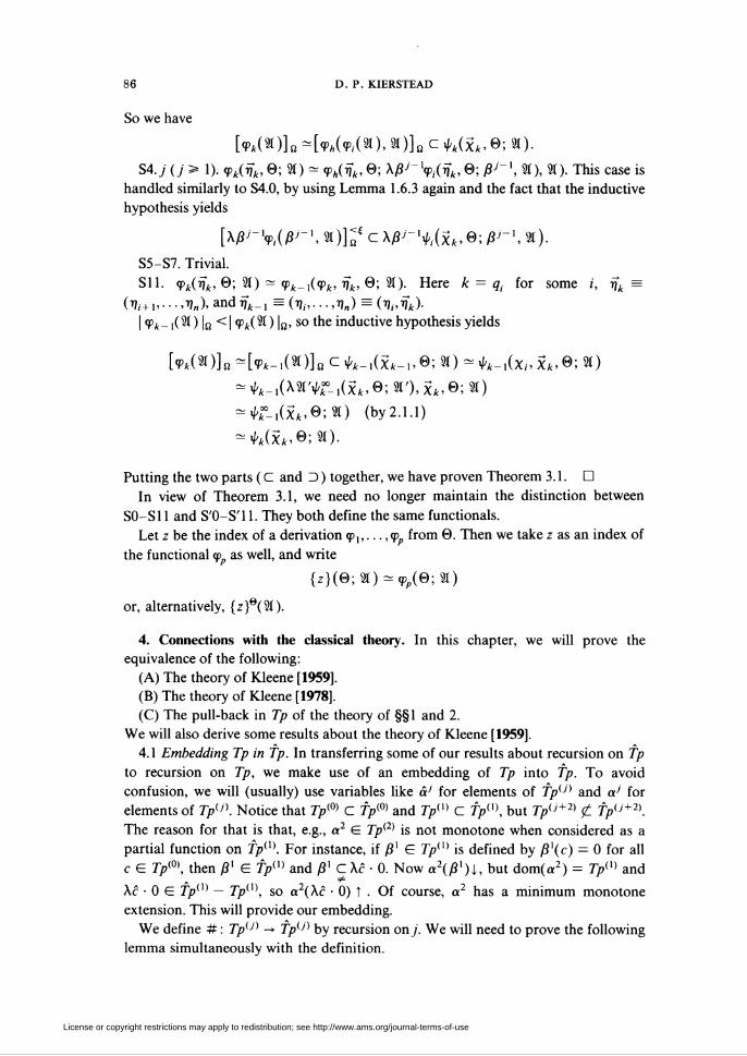
4.1 Embedding Tp in Tp. In transferring some of our results about recursion on Tp

to recursion on Tp, we make use of an embedding of Tp into Tp. To avoid

confusion, we will (usually) use variables like âJ for elements of Tp(J) and aJ for

elements of TpU). Notice that 7><0) C 7><0) and 7>(1 > C 7>(1), but Tp(J+2> j£ fpu+2).

The reason for that is that, e.g., a2 E Tp(2) is not monotone when considered as a

partial function on fp(X). For instance, if /?' E Tp(X) is defined by ß](c) - 0 for all

c E Tp(0), then ßx E fpiX) and ßx C Xc ■ 0. Now a\ßx)l, but dom(a2) = Tp(X) and

Xc ■ 0 E Tp(X) — Tpw, so a2(Xc • 0) î . Of course, a2 has a minimum monotone

extension. This will provide our embedding.

We define # : Tp(J) -» Tp<-') by recursion ony. We will need to prove the following

lemma simultaneously with the definition.


HIGHER-TYPE RECURSION THEORY y?

4.1.1. Lemma, (i) # is one-to-one.

(ii) If j 2* 1, then every #aj has the same domain, namely

{0J~X E Tp(J-X): {3ßJ~x E Tp(J~X))(#ßJ-x C /3^')}.

(iii) // âJ E TpU) then there is at most one aJ E Tp(J) such that #aJ C à1. D

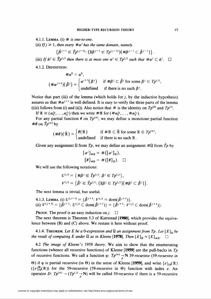
4.1.2. Definition.

#a° = a0,

, ...x/..v \aj+HßJ) if #/3> C/3^ for some/3^'e Tpu\(#aJ+x)(ßJ) <=*\ V ' F

[ undefined if there is no such ßj.

Notice that part (iii) of the lemma (which holds fory, by the inductive hypothesis)

assures us that #aJ+x is well defined. It is easy to verify the three parts of the lemma

((iii) follows from (i) and (ii)). Also notice that # is the identity on Tp<0) and Tp{X).

If 91 = (a¿°,... ,aJ„") then we write #91 for (#a¿°,..., #aJn»).

For any partial function 0 on Tpâ), we may define a monotone partial function

#0 on fp(a) by

(#0)(t)^{ö(3i) if #2t C3Í for some 31 E Tp(°\

{undefined if there is no such 91.

Given any assignment ß from Tp, we may define an assignment #ß from Tp by

[«y]#o = #([«ylo).

M#o=#([«]0)- n

We will use the following notations:

U(J) = {#ßJ E fp(J): ßJ E TpU)},

yU) = |/jy G fpU). /3ßj e TpU))(#ßJ C 0J)}.

The next lemma is trivial, but useful.

4.1.3. Lemma, (i) Uu+X) = {ßJ+x: VU) = dom(/3>+1)}.

(ii) Vu+X) = {ßJ+x: UU) C dom(ßJ+x)} = {ßJ + x: V^ C dom(/3>+1)}.

Proof. The proof is an easy induction ony. D

The next theorem is Theorem 5.3 of Kierstead [1980], which provides the equiva-

lence between (B) and (C) above. We restate it here without proof.

4.1.4. Theorem. Let E be a 0-expression and ß an assignment from Tp. Let [E]a be

the result of computing E under ß as in Kleene [1978]. Then [E]a - [E]#a. D

4.2 The image of Kleene's 1959 theory. We aim to show that the enumerating

functions (whence all recursive functions) of Kleene [1959] are the pull-backs in Tp

of recursive functions. We call a function <p: Tp(a) -^N 59-recursive (59-recursive inp

0) if N) will be called 59-recursive if there is a 59-recursive


88 D. P. kierstead

<p: Tpu) X Tp(a) -» N such that for all 91 E 7><0)p

D(%) = XßJ(p(ßJ,%).

We will see in §5 that we cannot code arbitrary finite sequences from 7p(7) as

elements of TpU) (we will have to move up to fpu+X)); but there is sufficient coding

capability for our immediate needs. The following definitions should be thought of

as being carried out over Tp (although they are formally the same as the correspond-

ing definitions over Tp from Kleene [1959]).

pt - the (/' + l)st prime,

(a0,. ..,a„_,)^ [] PÎ' (undefined if any a, is u ),;>Sn- i

« >*1).

(a),: — the largest n such thatp" divides a.

For y > 1 :

<aá,...,a>_1>-X^-,<a¿(^-,),...,<-1(i8J-,)>.

(ai)^\ßJ-l-{at(ßJ-l))r

These operators should really carry superscripts to indicate the type of their

arguments, but this seems to be entirely too pedantic. Clearly (via Lemma 2.2.4) all

of these functions and operators are recursive.

As we remarked above, these definitions may be used in either type structure. We

shall do so and use the same notation in both cases, relying on context to make the

distinction.

We do not, in general, have that ((âJ0,.. .,aJn))¡ = âj (e.g., ((0, u»0î). For-

tunately, we will only need to worry about these coding functions at arguments from

UU), and we do have the following:

4.2.1. Lemma. For aj, aJ0,...,aJnE Tp(J):

(i) <#<...,#<>=#<<...,«/,).

in) (#«;),.= #(«'),.

(m) «#<..., #<», = #«/.

Proof, (i) and (ii) are easily verified using Lemma 4.1.3 and the definitions, (iii)

follows from (i) and (ii) and the similar result from the classical theory. D

There is a good reason that we did not simply define these operators on Tp and

then look at their images under #. The image of a 59-recursive operator is not

usually recursive—it is defined too often. Fortunately, for "nice" operators (like

(—), etc.), the image is sufficiently close to being recursive. This is the motivation

for the next definition.

4.2.2. Definition. A 59-recursive operator D: Tp(a) -» (Tpu) ->N) is embeddablep

if there is a recursive operator D: fp(a) -* fp(J+ ° such that for all 91 E Tp(a)

/3(#3I) = #(Z)(3I)),



i.e., if the following diagram commutes:

Tp(o) " Í7>0)-»n)

l# i#

fp(a) 5. fpu+X)

(Recall that # is defined on all of (7>0)^N)—not just on Tpu+X)—and ifp

N) then #<p E Tpu+X).) If ¿ is associated with an embeddable opera-p

tor D (as above), then D is called an embedded operator. D

The operators (—,—,—) and ( — )¡ are embedded. While there will, in general, be

an infinity of embedded operators D associated with a particular embeddable D,

they will all agree on [/(o) and it is only there that we shall be concerned about their

values. Thus, there should be no ambiguity if we use the same notation for both D

and D (as we do with (— , —, — ) and ( — ),-). If the reader is bothered by this, he

may console himself by the fact that there will always be a natural choice of a

specific D.

For notational convenience, we define three more embeddable operators

Ins( — ,—,—), Del( —, — ) and Con( — ,—,—) which allow us to insert and delete

elements of coded sequences, and form concatenations.

4.2.3. Definition.

ímia,b,k)^l][pía)')-pÍ-( n />(a)-),i<k k<i<a

Dd(«,*)«(nfH-( n p\a)'A,i<k k<i<a

Cton(*. *,*)-( II/H'i n ¿H"V i<k ' V kî<b + a '

Con(a, b, k) codes the concatenation of the first k elements of (the sequence coded

by) a with (the sequence coded by) b. The extra parameter k is needed because this

particular coding scheme does not recognize a terminal string of zeros in a, which we

may wish to preserve.

Fory > 1 :

lns(aJ,ßJ, k) = XyJ-xlns(aJ{yJ-x), ßJ(yJX), k),

Deny, it) = Xy^Dehy^-1), it),

Con(aJ,ßJ, k) = XyJ-xCon(aJ(yJ-x), ßJ{yJ~x), k).

Clearly, these operators behave as desired on iy<y-7,0) (though not on all of

fpu'm). For example,

Ins(<#a¿, #a{, #a{), #ßj, l) = (#aJ0, #ßJ, #a{, #aJ2)

and

Del((#a¿, #a{, #aJ2), l) = (#aJ0, #a{).


90 D. P. KIERSTEAD

As usual, we will need operators u", d" which raise and lower the types of objects.

Both definitions may be applied in either type structure (and are standard on Tp),

but only d" will be embeddable.

4.2.4. Definition. uj+x and dj+x are defined by recursion ony.

Mo(«0)=Xy°[«0],

¿0(«') = «'(0).

For y > 1 :

uj+\^) = Xy\aJ(dj_liyJ))],

dj+x{a^x)=Xr-x[a^x{uj_x{y^x))].

We define uJj+k and dj+k by iteration.

uj(aJ) = dj{aJ) = aJ,

«/+*+V) = <í+1(^í-i(-«V)>-)).¿/+ft+lfy+*+1) = rfy+r(¿y«(... (¿y+*+i(a,+*+i))...)).

We will write simply u(aJ) and <¿(a>+1) for wj + 1(ay) and dj+x(aJ+x). D

The next lemma summarizes the basic properties of u and d. Clearly u and d are

recursive; they are also 59-recursive, but we do not need this fact.

4.2.5. Lemma. For all ßJ E Tp andßJ, yJ E Tp:

(i)d(u(ßJ)) = ßJandd(u(ßi)) = ß\

(ii) (forj ï* 1) ßJ C r ~ ¿(fr) C dir),(iii) ßJ C yJ « u(ßJ) C u(yJ).

Proof, (i) is proven by an easy induction on j. (ii) and the " =» " part of (iii)

follow from the monotonicity of recursive operators (see p. 80). The " <= " part of

(iii) follows by applying (ii) and then (i). D

In the next lemma, we are really interested in parts (i) and (iii). The other parts

make the proof go smoothly. Part (i) says that d is embeddable.

4.2.6. Lemma. For all ßJ, ßJ+ ' E Tp and all ßJ, ßJ+x ETp:

(i)#d(ßJ+x) = d(#ßJ+x),

(ii) #u(ßJ) C u(#ßJ),

(iii) ßJ+x E Uu+X)^d(ßJ+x) E Uij),

(i\)ßJ+x E Vu+X) =» difiJ+l) E V('\

(v)ßJ E VU)~u(ßJ) E V{J+X\

Proof. The proof is simultaneous, by induction ony. They = 0 case is trivial, so

lety^ 1.

(i) We first note that

dom(d(#ßJ+x)) = {yJ~x:u(yJ-x) E V(J)} (Lemma4.1.3)

^r'if'eK^") (ind, (v))

= dom(#d(ßJ + x)) (Lemma4.1.3).


HIGHER-TYPE recursion THEORY 91

Thus, it suffices to show that #d(ßJ+x) and d(#ßJ+x) agree on UU~X) (since

their values on F<7_1) are determined by their values on U(J~X\ by monotonicity).

Now

{#diß^)}i#yJ-*)={dißJ+1)}iyJ->)

= ßJ^(u(r-x)) = {#ß;+x}(#uiyJ-1))

= {#ßJ+x}(u(#r-x)) (ind,(ü))

= {d(#ßJ+x)}(#yJ-x).

(ii) By Lemma 4.1.3, dom(#u(ßJ)) = VU). Again, the values of u(#ßj) and

#u(ßj) on VU) are determined by their values on UU). Now

{#u{ßJ)}(#yJ) = HßJ)}(yj)

= ßid(yJ)) = {#ßJ}(#d(yJ))

= {#ßJ)idi#y')) (ind,(i))

= [ui#ßJ))i#yJ).

(iii) This is immediate from (i).

(iv) Let #yJ+x C ßJ+x. Then #d(yJ+x) = d(#yJ+x) C d(ßJ+x). (The contain-

ment is given by Lemma 4.2.5.)

(v) Suppose #yj C ßJ. Then #u(yj) C u(#yJ) C u(ßj). Conversely, u(ßJ) E

Vu+X) -> d(u(ßJ)) E VU) =* jS> E F0). D

Kleene [1959, p. 22] defined {z}59[a, a1,.. .,ar] to be

{*}s9((a)o>---> (ß)»„-i>(«%•••> (a,)*I-i,...>(a,')*,-i)

if z is the 59-index of a function of nj type-y arguments (for each y < r) and no

arguments of type > r; otherwise {z}59[a, a1,... ,ar] is undefined.

4.2.7. Lemma. Lei 0 = (0,,...,0,) oe a list of functions with 0,: 7>(0') -»N. Then,

for each r>0, there is a recursive functional x r such that for all z, a, a1,... ,ar E Tp,

Xr(#0; z,a,#ax,...,#ar) = {z}%[a, ax,... ,ar].

Proof. Let s = max{max tp(a,): t < /}. For each z, let rz be the maximum type of

any argument of {z}f9 (if z is an index for a function 59-recursive in 0). It will

suffice to define, for each r s» s — 1, xr(l>®; z> °> <*'>••■><*'') such that for all

z, a,ax,...,ar E Tp

X?(#®;z,a,#ax,...,#ar<,ur> + X,...,ur)^{z}%[a,ax,...,ar],

since we may then take, for r < s — 1,

xT-t{z,a,âx,...,âr,ur+x,...,us-x)

r/ô., . ii Ar\ ~ ] if z is a 59-index for a function

whose arguments have types < r,



92 D. P. KIERSTEAD

In what follows, we assume that r > s — I. We write 91 for (a, a1,.. .,ar), and

suppress the variables 0, which remain fixed throughout. We also omit the subscript

ronx-

X is defined by cases on z; but, as we are avoiding explicit use of indices whenever

possible, we state the case hypothesis in terms of the form of (z}59(93). Cases 0-9

correspond to the schemata S0-S9 of Kleene [1959].

Case -1. z or a is u, or z E N but z is not a 59-index for a function whose

arguments are of types < r. Take x(tj; z, Si) î .

Case 0. {z}59( — ) is obtained via SO.i, say with

{z}59(c, d, 93) - 0,(c, d, Xßi{e}59{ßJ, 93), Xßk{f}59(ßk, 93))

where y < rz and rz < k < s — 1. (There are really / separate cases here—one for

each 0,.) Clearly t, e, f, etc., may be extracted from z. Take

x(t,;z, à) ^ 0t[(a)o,(a)x,XßJ ■ V[e,Del(Del(a,0),0),ax,...,

&-x,Con((0J),âJ,l),âJ+x,...,âr],

X$k-Ti[f,Del(Del(a,0),0),âx,...,âr*,

dk + x(ßk),...,dk_x(ßk),ßk,ak+x,...,a'}].

The reason that y and k must be handled differently is that k = rf > rz, so when we

come to prove that x works, some of the a, with rz< i < rf may be u', but we will

need elements of t7(,) in these positions. These elements will be produced by

dk(#ßJ). All of this should become clear shortly.

Case 1. {z}59(c, 93) * c + l.TakeX(r/; z, 31) s* (a)0 + 1.

Case 2,3. Similarly.

Case 4. {z}59(93) - {g}59({h}59(%), 93). Take

xiw.z, â)-T)(g,Con«7,(/t,3i)>,a,l),â',...,âr).

Cose 5.

(z}59(0,93)-{g}59(93),

{z}59(c + 1, 93) - {/7}59(c, {z}59{c, 93), 93).

Take

X(T,;z,â)-

7,(g,Del(a,0),â,,...,âr) if(fl)0 = 0,

î,[/i,Con(((fl)0-- 1,t,(z, a -h 2, â1,...,«')>,

Del(a,0),2),â1,...,â'] if(a)0>0.

Caíe 6. (z}59(93) = {g}59i^8x) where 93 comes from 93, by moving the (A: + l)st

type-y variable to the front of the list. Take

xir, z, %) ^ v{g, a, âx,.. .,V~X ,lns(Del{âJ,0),{âJ)0, k), âJ+x,... ,âr).

Case 7. {z}59(y', c, 93) - y'(c). Take XiV, z, %) - {(âx)0}((a)0).



Case 8. {z}59(y>, 93) - yW^Wy7"2, yJ, 93)). Take

x(ti; z, t) « (a>)0[Xy>-2 ■ i,(A, a, a1,... ,âJ~\

Con(<y>-2>,â>-2,l),a'-1,...,<*')]•

Case 9. {z}59(a\ 93, 6) « {¿}59(93). Take

x(7};z,3l)-T)((a)0,Del(a,0),«1,...,âr).

This completes the definition of x- We now show that for all (z, 3Í) E Tp(0AX-■■■•r)

X"(#e;r,'a, #«',...,#«,«,u'»+,,...,n,,)'ai{x}»[*].

(C) We cannot use Lemma 2.1.1 since, in general, #(Xz31 ■ {z}f9[3I]) will not be

a fixed point of x (but the differences will be at arguments outside of rj(°Ai,. ,/■))

Instead, we show by induction on £ that for all (z, 3Í ) E Tp(0AX- -r)

x«(#0; z, #81) = w E N => {z)f9[3l] = w.

This is a slightly stronger statement than we need, since

X*(#8;z, a,#a\...,#ar-,ur-+\...,vir) = w ^X*i#®; ?,#%) = w,

but it is notationally more convenient. Again, we frequently suppress the variables

0. Suppose

xi(#0;^,#9i) = w.

We take cases on z. Let us consider four representative cases; the others are similar.

Case 0. {z}59(—) is as in the exemplary case treated in the definition of x- Here

(*) {z}i9[X]^0,((a)o,(a)x,XßJ-{e}59[Del(Del(a,0),0),ax,...,

*>-\ Con((ßJ),aJ,l),aJ+x,...,ar],

Xßk- {/}59[Del(Deu>,0),0), <*',...,«'%

dki+x(ßk),...,dk_x{ßk),ßk,ak+x,...,a]).

The reason that we may use dk+i(ßk) instead of ar'+i is that the value of {/}59[—]

is independent of the arguments of types between rz and k, since {/}59(—) has no

such arguments.

Now

w = xH#0; z, #31) = x(x<f, #0; *, #») = #*,(-)

where (—) is obtained by substituting x<£, #21 for tj, 31 in the definition of x (we

prefer not to rewrite it here). But #0, is only defined when its arguments come from

T/(0,o,y+i,*+o so there are yy+is yk+\ e Tp such that

»ti(")oÁah,yj+\yk+l) = ^,

#yJ+x C X0J • x<4(«. Del(Del(a,0),0), #ax,..., #a>_1,

Con((ßJ),#aJ,l),#aJ+x,...,#ar),


94 D. P. KIERSTEAD

and

#y*+1 C Xßk • x<£( /, Del(Del(a,0), 0), #«',..., #«r%

d!z+x(ßk),...,dk_x(ßk),ßk,#ak+x,...,#a').

By the inductive hypothesis and the fact that Con(-) and (— ) are embed-

dable (so Con«#/3>>, #«>, 1) = #Con«/^>, aJ, I)), we have that, for all ßJ E Tpu),

yJîßJ) = {#yJ^}i#ßJ) = x<ii-)

= {e}59[Del(Del(a,0),0),a1,...,a>-1,Con«/3Ô,^,l),a>+1,...,ar].

Further, using the fact that dk+j(—) is embeddable, we have that, for all ßk E Tp(k),

yfc+,(i8*) = {#Y*+.}(#i8*) = x<f(_)

= {f}59[Del(Delia,0),0),ax,...,ar',dk!+x(ßk),...,dk_x(ßk),

ßk,ak+x,...,ar].

Putting these last two equations into (*), we obtain

{z}59[%]^0t{{a)o,{a)x,yJ+x,yk+x) = w.

Case 4. Here {z}59[31] - {g}59[Con(({A}59[9i]>, a, 1), a',...,ar]. w = x(iz, #31)

= X<í(g,Con«x<í(/i, #2Í)>, a, 1), #ax,...,#ar). x<£ is undefined if either of its

type-0 arguments is u, so x<f('1> #21)1. By the inductive hypothesis

XÂ, #*) = {*}»[*]■

Using this, and the inductive hypothesis again, we have

X<£(g,Con(<x<f(/7, #3I)>, a, l), #«',..., #ar)

-{g}59[Con«{/7}59[3I]>,a,l),a,,...,^]-{z}59[31].

Case 6. Here

{z}59[%]^{g}59[a,ax,...,aJ-x,lns(Del{aJ,0),{aJ)o,k),aJ+x,...,ar].

Since (-)0, Ins(-) and Del(-) are embeddable (i.e., #(Ins(Del(a^,0),(«>)0, k)) =

Ins(Del(#a7,0), (#aJ)0, k)), the inductive hypothesis yields the result.

Case 8. This is just like Case 0, except that we do not have the problem of ry being

greater than rz to complicate things.

(D) One may now show, by induction on (z}59(—) (see Kleene [1959, p. 14]), that

for all (z, 3i)E Tp^°-X-•■■•r>

{*}»[»] =w =*xK(#®; z, a, #ax,...,#ar% ur<+1,...,ur) = w.

Again, we take cases on z. The cases are just the reverses of the corresponding cases

for "C ". The only place where the arguments ur*+' (instead of #ar* + i) could

possibly cause trouble is at Case 0. We sketch this case.

Case 0. {z}59(—) is as in the exemplary case treated in the definition of x- Since

{z}59(c, d, 93)1, we have that, for some yJ+x,

y'+l=X&- {e}59(/3>,93) = X/3^{e}59[Del(Del(a,0),0),a1,...,a>-1,

Con(</3y>, aJ,l),a'+',..., ar]



is total. Now re = rz (sincey «S rz), so the inductive hypothesis yields that, for each

ßJ E TpU),

Xxie,Del(Del{a,0),0), #ax,... ,#aJ~x, #Con{(ßJ), aJ,l),

#aJ+x,...,#ar*,ur'+x,...,ur)=yJ+x(ßJ).

Notice that j < rz is necessary in order for the left side of the last equation to be

meaningful.

Similarly, for some y*+1,

yk+x=Xßk-{f}59(ßk,%)

= W' {/}59[Del(Del(a,0),0),«',...,ar%

dk!+x(ßk),...,dk_x{ßk),ßk,ak+x,...,«']

is total. Now rf—k (since k > rz), so the inductive hypothesis yields that, for all

ßk E Tp(k\

X°°( /, Del(Del(a, 0)0), #«',..., #ar',

#dk2+x(ßk),...,#dk_x{ßk),#ßk,uk+x,...,ur)=yk+x{ßk).

Putting these facts together with the embeddability of Con( — ), ( — ) and dk+i( — ),

and substituting into the definition of x, we have that

x(xc°;#®;z,a,#OLX,...,#ar>,vtr*+x,...,ur) = w.

Finally, we apply Lemma2.1.1 to obtainx°°(#©;-) = was desired.

Why did we treat y and k differently in the definition of x? If we had not, we

would have needed to known that for all ßk

X°°(f,Del(Del(a,0),0),#ax,...,#ar',ur*+x,...,ur)=yk+x{ßk).

But this would not have followed from the inductive hypothesis. We needed #ßk in

the kth position, and we needed elements of U0) in the 7th position, for each i < k.

These elements were produced by dk(#ßk). D

4.2.8. Theorem. Let <p(31) be 59-recursive in 0. 77ie77 there is a recursive «//(©; 31)

such that for all 91 E Tp

«//(#©; #9t) ^<p(3I).

Proof. Say <p(31) is <p(a, ax, ßx, a4, /34). Let z be a 59-index of tp. With x4 as in

Lemma 4.2.7, set

«//(©; a, âlJ\ â\ ß4) - x4(0; z, a, <«', ßx), d\(à"), d\{à*), (à\ ß*)).

The result now follows from Lemma 4.2.7 and the embeddability of (— ) and

dk(-). U

Remark. Our ability to define xr, even when © might have arguments of types

> r, hinged on our use of ur+l. We had to be able to produce some type-r + i object

to be an argument for xf-\\ and we had to be able to use objects which were not in

U(r+,) since elements of U(-r+,) could only be produced if an element of U<-r+l+J)


96 D. P. KIERSTEAD

were available (for some y). If each of 0 were total, then we could have used 0 to

produce an element of i/(î+1). Thus the only reason for the added confusion of the

ur+1 is that we wanted the full generality of relativization of partial 0.

4.3 The 59-recursiveness of the pull-backs of recursive functionals. The proof of the

next lemma could be simplified somewhat by using Theorem LXI of Kleene [1963],

which provides for restricted substitution in 59-recursive functions. But there was a

great deal of machinery used to prove this result, and with very little extra work we

can avoid this machinery—all of the machinery is already a part of the computa-

tions of §1. The most general form of substitution (Theorem 4.4.3) will come out of

our work in this section and in Theorem 4.2.8.

Let us suppose that some reasonable Gödel numbering of y'-expressions has been

chosen. We denote the Gödel number of A by TA 1 .

For any O-expression E, let TE be the list of (formal) free variables of E in the

order in which they occur. Let 9i£ be a list of "informal" variables of the same

number and types as TE.

4.3.1. Lemma. For each list 0, there is a primitive recursive function i¡(z, e) such

that: if z is the index of a derivation from 0 and e is the Gödel number of a

O-expression E based on this derivation, then tr(z,e) is a 59-index for a function (rec.

in 0) of the variables 31 £ and for all 91 £ E 7>(a) (where a = ch(9I£))

{<n(z, e)}%(91£) « [£]a[r£/#*£]

(where ß is any assignment which assigns the functions #0 to the function variables of

E).

Proof.9 We will choose a 59-index p for w via the Second Recursion Theorem

(Kleene [1959, XIV]). For clarity, we will simply state what m(z,e) must be in terms

of p—which is only chosen after the fact.

We take cases on e. As always, we suppress 0.

Case — 1. z is not the index of a derivation or e is not the index of a O-expression

based on this derivation. Take 7r(z, e) to be 0.

From now on, assume that Case -1 does not hold. We state the rest of the case

hypotheses in terms of the form of E, where rE~* = e.

El. E is y°. Take -n(z, e) to be a 59-index of Xa[a].

E2. E is <Pj(A). Let E* be as in Definition 1.3.2, E2. Take ir(z, e) to be a 59-index

of X3I£ • {it(z, r£*n)}59(9í£). Let us spell this out a little more carefully (this once

only). First pick/such that {f}S9(d, 9i£) =* {d}59(%E). Now, using the 59-index/?

to be chosen for tt, choose h such that

{h}59{Ê)^{f}s9{{p}s9Íz,rE*"),%E),

and then take it(z, e) = h. We do not simply take ir(z, e) =¡ m(z, TE*^), because -n

would no longer be primitive recursive, nor even total.

9The proof consists of imitating the construction of the computation tree for E under S2[rt/#3I].

Since, under such an assignment, the construction of the tree is completely deterministic, we are able to

embody it in a 59-recursive function.



E4.X. E is {XßjA}(B). Similarly, take ir(z,e) to be a 59-index for X3I£-

(77(z,r5^n}59(3l£).

E4.1. E is yx(B). Take m(z, e) to be a 59-index for

X3t£-«,({W(z,r^)}59(3iB));

where ax is the first variable in 9i£.

E4-7 (y > !)• ̂ is y\B). Take tt(z, e) to be a 59-index for

X^^Xa^-^fz/^-2)1))^,^-2));

where aj is the first variable in 91E and aJ"2 is a new variable. (Notice that

2W-) = (2Í77, «;~2)-)

E5. E is 0. Take ir(z, e) to be a 59-index for 0 (as a function of no arguments—see

Kleene [1959, p. 3]).

E6 + , E6 — . Similar.

E6cs. E is cs(A, B, C). We use the fact that an index for strong definition by cases

may be obtained from indices of the fucntions and predicates involved (see Kleene

[1959, XVIII]). Take it(z, e) to be a 59-index for

>(z,r¿r)}59(9íB) if{w(z,^1)}59(3tj=0,

W^/Cyic) if{77(z,M1)}59(3iJ>0.X3I£

(Of course, e.g., by 91 ̂ we mean those arguments from 31E which, in 3t£, correspond

to the variables of A.)

El. Similarly to E4. y.

Now, once the 59-index p for m(z, e) (which was used throughout) has been

chosen via the Second Recursion Theorem, each value of ir(z, e) is specified in terms

of primitive recursive functions of p, z and e. Thus, 7r is primitive recursive.

It remains to show that tr does what was claimed.

(C) We show by induction on {z}(—) (see Kleene [1959, p. 14]) that, if z and e

are as in the statement of the lemma and {tr(z, e)}59(21£) = w, then [E]Q[Te/#%¡;] =

w. We take cases on the form of E. Let us consider only the case E4.y (y > 1).

E4.y (j > 1). The inductive hypothesis yields that for each aj~2 E Tp^J~2)

{v(z,r B(r-2y)}59{KB,aJ-2) =[B{yJ-2)]a[yJ-i/#aJ-,jB/#vB].

Thus

¿(XaJ-2 ■ {.{z,rB(r-2+y)}jKB,a;-2))

- {#aJ}([B]a[rB/#KB)) ~[E]a[TE/#%E].

(D) We show by induction on £ =| E\q,Te//#%eX that for all 31 £ E Tp^\ if

[£]a[r£/#wE] = w> tnen {î2, e))59(2l£) = w. Again, we consider only one case.

E4.y (j > 1). Since #aj is only defined on VU~X), we have some aj~x E Tpu~X)

such that #aJ~x C [B]^T /#a x and aj(a'~x) = w. That is to say, for all aj~2 E

TpU-*>,

[B(yJ~2)]afyJ-i/#aJ->,rB/**B] = «;-V"2).


98 D. P. KIERSTEAD

Now the inductive hypothesis applies to yield

a>-l = )*l-2-{w(z,rB(y'-*y)}jiXB,«'-*).

Thus

{v(z,e)}59(%E) = a\aJ-x) = w. D

4.3.2. Theorem. Let 0 be a fixed list of functions on Tp. If <p(®; 91) is a recursive

functional, then there is a function «//(3Í), 59-recursive (uniformly) in 0, such that for

all 91 E Tp(a)

^(3i) ~ <p(#e-, #3i).

Proof. Consider a derivation <p,,... ,(0) ->N. Let 0 be a list of functions on Tp. Then the

following are equivalent:

(i) (a),

^(#0;#3i)^«p(3t). D

We call such a «// a recursive functional corresponding to <p.

4.4 Some results in Kleene's 1959 theory. While we have never seen the theorems of

this section in print, the facts are undoubtedly known to any researcher in the field.

It is our belief that the development above makes them particularly natural. For

simplicity, we consider only the unrelativized versions.

The import of the next theorem is: If <p(9l) is 59-recursive with 3Í = (a/1,... ,aJn")

and r — maxtp(3I) > 1, then for each 31 E 7/7(o) for which <p(3I)l, the value of

<p(9t) is determined by the type-0 arguments and the value of the higher type

arguments at certain minimum subsets of their domains; moreover, if j¡ = r then the

subset of dom(a/') has strictly smaller cardinality than dom(a/')-

Recall that {z}( —) is the recursive function whose derivation has index z and

(z}59( —) is the 59-recursive function with 59-index z.

4.4.1. Theorem (Use lemma). Let 93 E Tp(0A ■•0) and 31 = (a{\...,aJ„") E 7>(o)

with r — max tp(%) > 1 and each j¡ > 1. Suppose that (e}59(93, 91)1. Let (z}( —) be a

recursive function corresponding to {e}59( — ). Then there are minimum partial subfunc-

tions X = (xi1,.. • ,XJ„*) c 3Í such that {z}(93, #£)!, whence, for all 91* E 7>(o),

I C 31* =» {e}59(93, 91*) = (z}(93, #3E) « {e}59(93, 31).

Moreover, Card(dom(x/')) * ^r-2 (finite if r = 1).

Proof. Let <p,,...,<p = (z}( —) be the derivation indexed by z. We prove by

induction on £ = | E \Q that, if £ is a O-expression all of whose free variables have

type < r, and ß assigns #a/' to y/' and makes all of its other assignments from

various i/(7)'s, and [E]a 1, then there are S, as in the statement of the theorem, such



that

[Ë]Qlyp/#x{<,...,yi«/#x',»] ~ [E]si-

The theorem will follow by applying this to the O-expression <ppC¡8, y/1,.. .,y¿").

We take cases on the form of E, considering only the E4.y (y > 1) case (the others

are trivial).

E4.y (y > 1). E is ßJ(D). Note that y < r. Since ß makes its assignments from U,

there is a ßj~ ' E Tpu~X) such that #ßj~ ' C [D]q£. Let y^"2 be a new variable. For

eachSJ'2 E Tp^~2\

[D(yJ-2)]^/#s^n-

Associated with each oj~2 E Tpu~2\ we have (via the inductive hypothesis) sub-

functions xJi's as in tne theorem.

If ßj is not one of y/< we may take x/' = U {x/>: o E Tpu~2)}. Then

#/3^"1 C [Z>]aï>/*x/<]

so

[/3^fl)]0[Y/V#x/i]l(and^[£]a).

Clearly any choice for x/' which did not contain all of the x/>'s would cause one of

the subcomputations to diverge, whence the entire computation would also diverge.

Thus, our choices x/' were minimum.

Finally,

Card(Dom(x/')) < 2 Card(Dom(x/;6)) < Sy-2 ■ lr_2 < 2r_2.Í6J><'"2)

If /S7 is y/' for some /', then we must include the additional value xJi'ißJl) —

a{'(ßJ~1)- □

Remark. The proof of Theorem 4.4.1 is no more than the formalization of the fact

that the computation tree for [E]ü has cardinality < 2r_2 and the value of [E]ü is

determined by the values of a/' at vertices of the form y/'(B) on the tree.

4.4.2. Lemma (In the unextended theory). Let j 3= 1 and maxtp(a) <j. The

predicate

R(aJ) » VßJ-xi<xJißJ-x) = O)

is not 59-semirecursive in any 93 E Tp(a).

Proof. Suppose that, for some 59-recursive <p and some © E Tp(a),

R(aj) ~<p{aj, 93)1.

Then <p(Xßj~x • 0, 93)1 and (by the use lemma) this fact is determined by the values

of XßjX ■ 0 on at most 1_2 arguments (finitely many if y = 1). Now Card(Tp(J~X))

= !■_, so there is a 8j E TpU) which is 0 at these arguments and 1 at some other

element of Tpu~ ". Then (p(SJ, 93)1 and -,R(8J), which is a contradiction. D

One direction of the next theorem is Theorem 16.4 of Kechris and Moschovakis

[1977], where it is attributed to Kleene. Both directions become trivialities in the

current setting.


100 D. P. KIERSTEAD

4.4.3. Theorem (y > 1). Let d(ßj, 93) be 59-recursive, a — ch(93), and suppose

there is some 930 E 7jP(o) such that Xßj6(ßJ, 930) is total. Then the following are

equivalent:

(i) For each 59-recursive ^0(yj+l, 93, Ê) there is a 59-recursive «//(93, 6) such that,

for values o/93 and S with Xßj6(ßJ, 93) roía/,10

«//(93,e)-ô(X/3>0(/3^,93),93,6).

(ii) maxtp(93)>y + 1.

Proof, ((ii) => (i)) Let a* be one of the variables in 93 of type k>j+ 1. Choose

recursive «//0 and ^corresponding to «//0 and 0 respectively. Set

0O(/K 93) - 0"(/3>, 93) + cs{{dk+x(ak)}(ßJ),0,0).

Now, for all 93 E 7>(0) with XßJ6(ßj, 93) total and all j8'' G Tpu),

60(#ßj, #93) * 0(#/3', #93) « 0(/3>, 93).

Thus, F0) C Dom(X/3'0o(/K #93)). On the other hand, since rff+l is embeddable,

Dom(dk+ ,(#o*)) = F<A Thus Dom(X/3'0o(/K #93)) = F°>.We have shown (via Lemma 4.1.3) that, for values of 93 E Tp(a) with XßJ6(ßJ, 93)

total,

Xß%(ßJ, #93) = #iXßj6{ßJ, 93)).

Thus, taking

«R93, Ê) - j0{Xß%(ßJ, 93), 93, 6),

we have, for all 93 E r/>(0) and © E 7><T> with XßJß(ßJ, 93) total,

¿(#33, #©) - t0(XßJ6{ßJ, 93), 93, g).

By Theorem 4.3.3,

«¿(93, 6) = *(#»,#©)

is the desired 59-recursive function.

((i) =» (ü)) Suppose max i/>(93) <y and 93 0 E 7>(o) is such that XßJ0(ßJ, 930) is

total. By Lemma 4.4.2, the predicate V8J~x(ßJ(8j~x) = 0) is not 59-semirecursive in

So-Let

*o(yJ+\ßJ,*)~yj+i{™j-i0 ifW-') = o|\ [undefined otherwise /

Then %(yJ+\ ßJ, 93)1 « V8j-x(ßJ(8J~x) = 0). Now suppose that for all ßJ

tißJ, 930) « ^{XßJOifi, 930), /3>, 930).

Where «// 59-recursive, then V8J~x(ßJ(8J~x) = 0) would be 59-semirecursive in 930,

which cannot be.

l0If we did not require the existence of some 390 for which \ßJB(ßJ, 390) is total, this condition would

be trivially satisfied by any «|/(33, @).



Remark. The previous theorem formalizes the fact that: the substitution principle

breaks down if the object being substituted for is used to test the totality of some

computed function, and this problem may be circumvented if another object, of

sufficiently high type, is available to perform this test.

5. Enumeration, s — m — n and second recursion theorems on Tp. We now leave

Tp behind and work entirely within Tp. In order to prove the Enumeration

Theorem, we will need some coding apparatus. As we now mentioned in §4.2, we

cannot code sequences from TpU) as elements of Tp(j\ The problem is that the

recursive functions are all monotone. For example, (u, u), (u, 1) and (1, u) would

all have to receive different codes in Tp(0), whence at least two of them would receive

different codes a, b E N; but then monotonicity would require that (1,1) = a and

(1,1)= o, which cannot be. In order to have acceptable codes for sequences from

Tpu\ we must move up to Tpu+X).

5.1 Definition. We define the coding and decoding operators (a{,...,aJn) and

(a7),- by recursion ony.

(«0,..,«°>=Xy°

n ify° = 0,

a0 ify° = i,\<i<n,

0 ify°>7i,

(«')-«'(,),

U > 1)

<a/,...,a/,>=XyJ

ifd¿-x((r)x) = o,

«i{(yJ)2)

0

ifd¿- '((y^),) =/,!</<„,

itdi (aV),)>«,«J+l«H-lii),yJ-% D(a7+1),. = Xy7-

5.2 Lemma. If I < / < n then

««/,...,<», = «/.

Proof. Induct ony. D

We need one operator to alter coded sequences. Alt(a7+1, ßj, i) will replace the

/th entry in the sequence (coded by) aj+x by ßJ.

5.3 Definition.

max{i,ax{0)} ify° = 0,

Ait(a\i8°,i)=XY0- ax{n)

ß°

if 1 < y°

if 1 < y°

nî,

0">1)

Alt(aJ+x,ßJ, i) = AyJ

max{7,a7+1«M¿-'(0)»}

aJ+x(yJ)

ßJ((yJ)2)

ifd¿~xi(yJ)x)=0,

ifl<d¿-x{(yJ)x) = n*i,

ifl<d¿~x({yJ)x) = i, D


102 D. P. KIERSTEAD

Clearly Alt is recursive and behaves as desired; e.g.,

Alt(<«>, a{, a¡), ßJ, 2) = (a{, ßJ, a{)

and

Alt(<a|, «i, a&, ßJ, 5) = (a{, a{, a{, XyJ~x ■ 0, ßJ).

We now come to the Enumeration Theorem. We ask the reader to notice that, in

defining the enumerating functional for functions tp of arguments having types < r

(r > 0) recursive in 0 where each of 0 has arguments only of types < r — 1, S4.y is

only used withy *£ r — 1. (We will need this fact in the proof of Theorem 5.5.)

It is convenient to use a combination of the syntactic system of §1 and the

semantic system of §2.

5.4 Lemma. Let r > 0 and 0 = (0,,... ,0,), where each 0, has only arguments of

types < r — 1. For each q ands, there is a recursive functional

sp{®;z,e,ax,...,ar-x,a[-x,...,aq-x,arx,...,ars)

such that, if

(i) z is the index of a derivation <px,... ,<p from 0, and

(ii) e is the Godel number of a O-expression E based on tp,,...,tp whose free

variables of types r — 1 and r are among y[~x,..., yl~l, y(,..., y¡, and

(iii) ß is the assignment obtained from ax,...,ar~x, arx~x,...,aq~x, a[,...,ars by

assigning: ar~x to the formal variable y[~ ', ar¡ to y[, and, for j < r — 1, (aJ+ ' ). to y/,

then

t{[G]Q;z,e,a\...,a'-\a[-\...,aq-l,a[,...x)~[E]Q-,

and «//([0]n; z,e,...) Î if z and e are not as above.

Proof. For simplicity, we suppress 0 and write

%=(a\...,a'-\ar{-\...,aq-x,<x[,. ..,<).

We define xiv, z, e, 31) and show that «// = x°° has the required properties. The

definition is by cases on the form of E (where T ET — e).

Case 0. z and e are not as specified in (i) and (ii) above. Take x(rç; z, e, 91) to be

undefined.

El. E is y,°. If r = 1 (so 1 < i < q) take x(i; z, e, 31) - a0. Otherwise, take

x(T,;z,e,3I)-(a1),.

E2. E is <PjiA). Let E* be as in Definition 1.3.2, E2. Take xiv, z,e, 31) -

t,(z, r£*\3I).

E4.X. E is {XßJA}iB). Takex(T); z, e, 31) a t,(z, r SÂ |n , 31).

E4.y. E is y/(t3). We supposey > 1 (y = 1 is almost identical).

If y = r (and similarly if y = r — 1) take

x(T,;z,e,3t)-<(xr-2-7,(z, r73(Yr2)n ,ax,...,ar-2,

Alt(a^x,Sr'2,k),arX,...,ar-\otrx,...,al))

where y¿"2 is the first type-(r — 2) variable not free in B.



If 1 <j < r - 1, take

x(r/; z,e, 91)

îaJ+x)[x8J-2 -V(z,rBÍy¿~2Y ,ax,...,aJ-2,Altia^-x,8J-2,k),

aJ,...,ar~x, arx~x,... ,aq~x, arx,... ,arJ\

where y/~2 is the first type-(y — 2) variable not free in B.

E5, E6. Obvious.

E7. Similarly to E4.y. (If 0, has a type-(r — 1) argument, then 0, is "essentially" a

type-r object.)

This completes the definition of x-

Now let «/<(z, e, 3Í) have all of the properties claimed for «// except, possibly,

recursiveness. It will suffice to show that, for all z,e, 91,

«Mz,e,9i)-x°°(2,e,3r).

(D) It is easy to see that XzeSI • xiñ z, e, 91) C «p, whence, by Lemma 2.1.1,

x°°c£( C) We show, by induction on£=\E\a, that, if z and e = r E1 are as specified in

(i) and (ii) above and ß is the asignment obtained from 9Í, and [E]a 1 then

x°°(z,e, 91)-[£]a(-«Hz, e,3i)).

We consider only the case E4.y (1 <j<r— 1), the others being similar or trivial.

E4.y (1 <j < r — 1). E is y/(v3). Now [y/]a = (aJ+x)¡, so it suffices to show that

(•) [B]t( CX8J-2 ■ xM(z,TBÍy¿-2y ,a\-..,«j-2,AltiaJ-\8J-\k),

aJ,...,ar-x,arx-x,...,aq-x,arx,...,a¡).

Now [B]t( = XS7"2 ■ [5(Yr_2)Ja\Vv*'-2] and ^k'2/^'2] is the assignmentobtained from (a1,... ,Alt(aJ~', 8J~2, k),.. .,ars), so (*) follows from the inductive

hypothesis. D

5.5 Theorem (Enumeration Theorem). For each a and each 0 = (0,,...,0,),

there is a recursive functional «//(©; z, 31) (where ch(3i) = a) such that, if z is the

index of a functional tp(0; 31), then for all 0 and 3Í

«//(©; z, 9t)-<p(0;3I)-{z}e(Si).

Moreover, if max tp( 91 ) < r and each argument of each of 0 has type < r — 1, then «//

may be defined entirely in the theory of types < r with S4. j used only with j < r — 1.

( In particular, no functional in the derivation of «// will have type-r arguments other

than those of «//, and none of type > r.)

Proof. We have only to code up the type-y arguments of «// (for j < r — 2) as

type-(y + 1) objects and substitute them into the enumerating function of Lemma

5.4. This uses S4.k with k<j + 1 < r — 1. The construction in Lemma 5.4 also

used S4. k only for k *£ r — 1. D


104 D. P. KIERSTEAD

As usual (see Kleene [1959, XIII, XIV]) we have:

5.6 Theorem (s — m — n Theorem). For each m > 0, there is a primitive recursive

function sm(z,ax,...,am) such that, if z is the index of a recursive function

{z}(ax,.. .,am, 93) and ax,...,am E N, then for all 93

{sm{z,ax,...,am)}{%)^{z}{ax,...,am,S8). □

5.7 Theorem (Second Recursion Theorem). Let «//(*, 21) be recursive. Then

there is an e EN such that for all 91

{e}(3I)-,//(e,3I).

Beyond this point, it is not clear whether Tp possesses an interesting recursion

theory. In particular, monotonicity requires that all recursive (total) predicates be

constant. There may be some interesting results about the semirecursive predicates

on Tp, but the principal value of recursion over Tp is the setting that it provides for

studying 59-recursion over Tp.

6. The relationship with some other theories. As we mentioned in §0, the system

which we have developed here is very similar to that of Platek [1966]. Platek wished

to develop a recursion theory on a (nearly) arbitrary collection Ob of "objects" (i.e.,

basic elements). His basic operation was that of taking the least fixed point of a

recursive functional F(tj; x). This required him to consider functionals whose

function arguments might not be total. Perhaps, he suggested, a larger class of

functions on Ob could be obtained if one also allowed these F to be defined as the

least fixed points of type-3 functionals Í>(F, tj; x). This required functionals 5> whose

type-2 arguments F were partial, and moreover, F might be defined on some partial

type-1 arguments. Continuing in this manner, he arrived at his hereditarily consistent

functionals HC. Platek's Reduction Theorem shows that there is no need to go up

through the entire structure of HC—the same recursive functions of objects are

obtained if one stops at level 2 (i.e., F(tj; xj) and performs recursions at that level.

Platek obtained an image of Kleene's 1959 theory by considering recursion on

Ob = N and associating 7/>(n) with a certain subset of the unary functions at the «th

level of HC. Thus the partial functionals entered the picture as arguments with

which to perform recursions—not as the basic objects of the theory.

Kechris and Moschovakis [1977] obtained Kleene's 1959 theory by taking Ob = Tp

and only going up to level 2 in HC (which the Reduction Theorem tells us is far

enough). For this reason, "partial objects" do not occur in their system.

We arrived at Tp in an attempt to provide a semantics for Kleene's 1978

computations. Essentially, it became clear that recursive functions of higher type are

not naturally limited to total arguments—even at the lowest level. This accounts for

the presence of u in Tp^0); u has no counterpart in HC.

Thus, while HC and Tp may appear to be very similar, the role of HC in Platek's

theory is significantly different (at least conceptually) from that of Tp in our theory.

Conceptually, our system is much closer to that of Kechris and Moschovakis [1977]

than to that of Platek [1966].



Within all of these theories is that of Kleene [1959]. That this theory may be

obtained by such varied means says something about the soundness of the original

system.

References

A. S. Kechris and Y. N. Moschovakis

[1977] Recursion in higher types, Handbook of Mathematical Logic, K. J. Barwise, Editor,

North-Holland, Amsterdam, pp. 681-737.

S. C. Kleene

[ 1952] Introduction to metamathematics, North-Holland, Amsterdam.

[1959] Recursive functionals and quantifiers of finite types. I, Trans. Amer. Math. Soc. 91, 1-52.

[1963] Recursive functionals and quantifiers of finite types. II, Trans. Amer. Math. Soc. 108,

106-142.

[1978] Recursive functionals and quantifiers of finite types revisited. I, Generalized Recursion

Theory. II, J. E. Fenstad, R. O. Gandy and G. E. Sacks, Editors, North-Holland,

Amsterdam, pp. 185-222.

[1980] Recursive functionals and quantifiers of finite types revisited. II, The Kleene Symposium,

K. J. Barwise, H. J. Keisler and K. Kunen, Editors, North-Holland, Amsterdam, pp.

1-29.

[to appear] Recursive functionals and quantifiers of finite types revisited. III.

D. P. Kierstead

[1980] A semantics for Kleene's j-expressions, The Kleene Symposium, K. J. Barwise, H. J.

Keisler and K. Kunen, Editors, North-Holland, Amsterdam, pp. 253-366.

R. A. Platek

[1966] Foundations of recursion theory, Ph.D. Thesis, Stanford University, Stanford, Calif.

Daniel Wagner Associates, Station Square One, Paoli, Pennsylvania 19301

Documents

SYNTAX AND SEMANTICS IN HIGHER-TYPE … · transactions of the american mathematical society Volume 276, Number I, March 1983 SYNTAX AND SEMANTICS IN HIGHER-TYPE RECURSION THEORY1