Synchronous Machine Excitation System, Vision · PDF file162 -036 CW 3 SYNCHRONOUS MACHINE TURBINE-GOVERNING SYSTEMS The conventional primary energy sources used for electrical

Phase to Phase BV

Utrechtseweg 310

Postbus 100

6800 AC Arnhem

The Netherlands

T: +31 (0)26 352 3700

F: +31 (0)26 352 3709

www.phasetophase.nl

Synchronous Machine Turbine-Governing Systems Vision Dynamical Analysis

Manual

16-036 CW

May 11, 2016

i 16-036 CW

Copyright Phase to Phase BV, Arnhem, the Netherlands. All rights reserved.

The contents of this report may only be transmitted to third parties in its entirety. Application of the copyright notice

and disclaimer is compulsory.

Phase to Phase BV disclaims liability for any direct, indirect, consequential or incidental damages that may result

from the use of the information or data, or from the inability to use the information or data.

ii 16-036 CW

CONTENTS

1 Introduction ............................................................................................................................ 1

2 Abbreviations .......................................................................................................................... 1

3 Synchronous Machine Turbine-Governing Systems ............................................................ 2 3.1 Speed Governing ........................................................................................................................... 2 3.2 Turbine and Governing System Implementation ......................................................................... 4 3.3 Per Unit System ............................................................................................................................. 4

4 Steam Turbine Models ........................................................................................................... 5 4.1 Type TGOV1 SMTGS ...................................................................................................................... 5

4.1.1 TGOV1 - Parameters ............................................................................................................... 5 4.1.2 Parameter Restrictions ........................................................................................................... 5

4.2 Type IEESGO 1973 SMTGS ........................................................................................................... 6 4.2.1 IEESGO 1973 - Parameters .................................................................................................... 6 4.2.2 Parameter Restrictions .......................................................................................................... 6

4.3 Type IEESGO 2003 SMTGS ........................................................................................................... 7 4.3.1 IEESGO 2013 - Parameters ..................................................................................................... 7

4.4 Type IEEEG1 SMTGS ..................................................................................................................... 8 4.4.1 IEEEG1- Parameters ............................................................................................................... 8 4.4.2 Parameter Restrictions .......................................................................................................... 9

4.5 Type LCFB1 Outer-Loop MW Controller ....................................................................................... 9 4.5.1 LCFB1- Parameters ................................................................................................................. 9

5 Gas Turbine Models ............................................................................................................. 10 5.1 Type GAST SMTGS ...................................................................................................................... 10

5.1.1 GAST - Parameters................................................................................................................ 10

6 Example ................................................................................................................................. 11 6.1 System description ....................................................................................................................... 11 6.2 Dynamic study ............................................................................................................................. 14

6.2.1 Dynamic case ........................................................................................................................ 14 6.2.2 Expected behaviour ............................................................................................................... 15 6.2.3 Simulation ............................................................................................................................. 15 6.2.4 Simulation results ................................................................................................................. 16

7 Bibliography .......................................................................................................................... 19

1 16-036 CW

1 INTRODUCTION

The Dynamic module of the Vision Network Analysis software is developed for the analysis of

electromagnetic transients. For a correct representation of synchronous generators both the excitation

system and the prime mover including its governing system need to be modelled. This document

provides a description of the turbine and governing system models implemented in the Vision Network

Analysis software. Those models are selected to be suitable for use in large-scale system stability studies.

The parameters provided as default must be considered as sample data only, the default parameters are

neither typical nor representative.

The outline of this report is as follows: first, a general description of the turbine and governing systems

is provided in Chapter 3. The implemented steam turbine models are presented in Chapter 4 together

with their default parameters and possible parameter restrictions. The implemented gas turbine is

treated in Chapter 5. Finally, an example of a dynamic study for a small industrial network is provided.

This manual is applicable to the Vision Network Analysis version 8.7.1 or higher.

2 ABBREVIATIONS

AGC Automatic Generation Control

ESM Excitation System Model

SMTGS Synchronous Machine Turbine Governing System

pu per unit

RMS Root Mean Square

AVR Automatic Voltage Regulator

2 16-036 CW

3 SYNCHRONOUS MACHINE TURBINE-GOVERNING SYSTEMS

The conventional primary energy sources used for electrical power generation are typically of hydro or

thermal nature. The prime mover converts these sources of energy into mechanical energy, which is

then used to drive the synchronous generator. Thermal energy can be obtained from nuclear or fossil

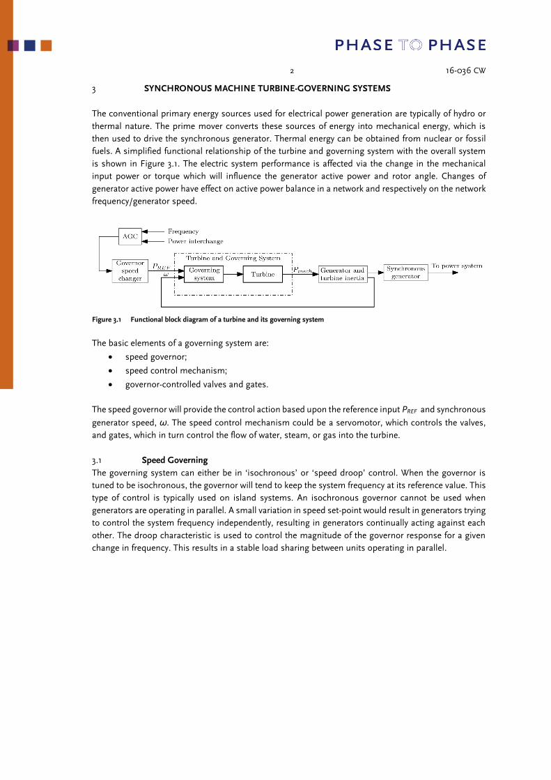
fuels. A simplified functional relationship of the turbine and governing system with the overall system

is shown in Figure 3.1. The electric system performance is affected via the change in the mechanical

input power or torque which will influence the generator active power and rotor angle. Changes of

generator active power have effect on active power balance in a network and respectively on the network

frequency/generator speed.

Figure 3.1 Functional block diagram of a turbine and its governing system

The basic elements of a governing system are:

speed governor;

speed control mechanism;

governor-controlled valves and gates.

The speed governor will provide the control action based upon the reference input PREF and synchronous

generator speed, ω. The speed control mechanism could be a servomotor, which controls the valves,

and gates, which in turn control the flow of water, steam, or gas into the turbine.

3.1 Speed Governing

The governing system can either be in ‘isochronous’ or ‘speed droop’ control. When the governor is

tuned to be isochronous, the governor will tend to keep the system frequency at its reference value. This

type of control is typically used on island systems. An isochronous governor cannot be used when

generators are operating in parallel. A small variation in speed set-point would result in generators trying

to control the system frequency independently, resulting in generators continually acting against each

other. The droop characteristic is used to control the magnitude of the governor response for a given

change in frequency. This results in a stable load sharing between units operating in parallel.

3 16-036 CW

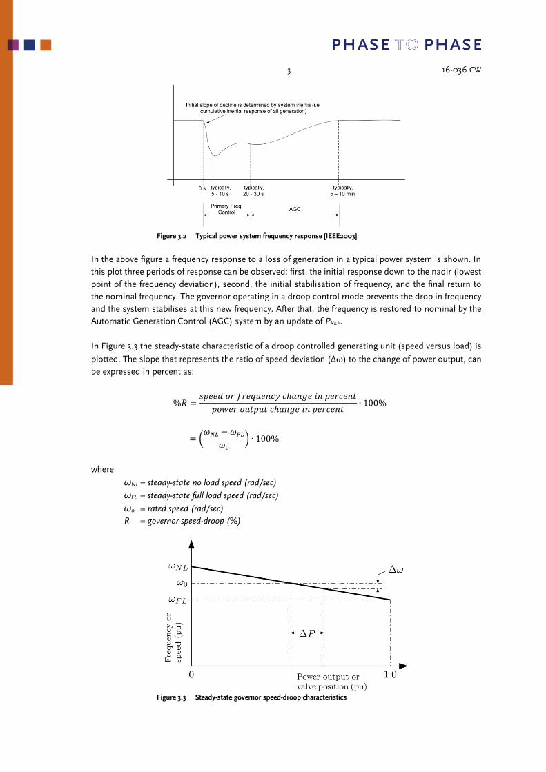
Figure 3.2 Typical power system frequency response [IEEE2003]

In the above figure a frequency response to a loss of generation in a typical power system is shown. In

this plot three periods of response can be observed: first, the initial response down to the nadir (lowest

point of the frequency deviation), second, the initial stabilisation of frequency, and the final return to

the nominal frequency. The governor operating in a droop control mode prevents the drop in frequency

and the system stabilises at this new frequency. After that, the frequency is restored to nominal by the

Automatic Generation Control (AGC) system by an update of PREF.

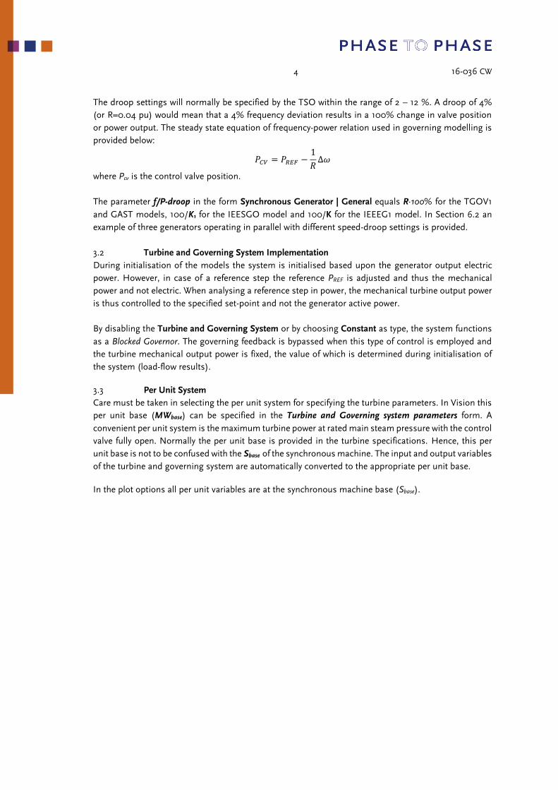
In Figure 3.3 the steady-state characteristic of a droop controlled generating unit (speed versus load) is

plotted. The slope that represents the ratio of speed deviation (Δω) to the change of power output, can

be expressed in percent as:

%𝑅 =𝑠𝑝𝑒𝑒𝑑 𝑜𝑟 𝑓𝑟𝑒𝑞𝑢𝑒𝑛𝑐𝑦 𝑐ℎ𝑎𝑛𝑔𝑒 𝑖𝑛 𝑝𝑒𝑟𝑐𝑒𝑛𝑡

𝑝𝑜𝑤𝑒𝑟 𝑜𝑢𝑡𝑝𝑢𝑡 𝑐ℎ𝑎𝑛𝑔𝑒 𝑖𝑛 𝑝𝑒𝑟𝑐𝑒𝑛𝑡∙ 100%

= (𝜔𝑁𝐿 − 𝜔𝐹𝐿

𝜔0) ∙ 100%

where

ωNL = steady-state no load speed (rad/sec)

ωFL = steady-state full load speed (rad/sec)

ω0 = rated speed (rad/sec)

R = governor speed-droop (%)

Figure 3.3 Steady-state governor speed-droop characteristics

4 16-036 CW

The droop settings will normally be specified by the TSO within the range of 2 – 12 %. A droop of 4%

(or R=0.04 pu) would mean that a 4% frequency deviation results in a 100% change in valve position

or power output. The steady state equation of frequency-power relation used in governing modelling is

provided below:

𝑃𝐶𝑉 = 𝑃𝑅𝐸𝐹 −1

𝑅∆𝜔

where Pcv is the control valve position.

The parameter f/P-droop in the form Synchronous Generator | General equals R∙100% for the TGOV1

and GAST models, 100/K1 for the IEESGO model and 100/K for the IEEEG1 model. In Section 6.2 an

example of three generators operating in parallel with different speed-droop settings is provided.

3.2 Turbine and Governing System Implementation

During initialisation of the models the system is initialised based upon the generator output electric

power. However, in case of a reference step the reference PREF is adjusted and thus the mechanical

power and not electric. When analysing a reference step in power, the mechanical turbine output power

is thus controlled to the specified set-point and not the generator active power.

By disabling the Turbine and Governing System or by choosing Constant as type, the system functions

as a Blocked Governor. The governing feedback is bypassed when this type of control is employed and

the turbine mechanical output power is fixed, the value of which is determined during initialisation of

the system (load-flow results).

3.3 Per Unit System

Care must be taken in selecting the per unit system for specifying the turbine parameters. In Vision this

per unit base (MWbase) can be specified in the Turbine and Governing system parameters form. A

convenient per unit system is the maximum turbine power at rated main steam pressure with the control

valve fully open. Normally the per unit base is provided in the turbine specifications. Hence, this per

unit base is not to be confused with the Sbase of the synchronous machine. The input and output variables

of the turbine and governing system are automatically converted to the appropriate per unit base.

In the plot options all per unit variables are at the synchronous machine base (Sbase).

5 16-036 CW

4 STEAM TURBINE MODELS

Large steam turbines are commonly used in the large fossil fuelled power plants. The steam turbine

converts stored energy (boiler) of high pressure and high temperature steam into rotating energy, which

in used to drive the generator. In the models described below the boiler is treated as an infinite and

constant source of steam, boiler dynamics are thus neglected.

Steam turbines normally consist of two or more turbine sections coupled in series. Currently only

tandem compound turbines are modelled, i.e. all turbine sections are on the same shaft.

4.1 Type TGOV1 SMTGS

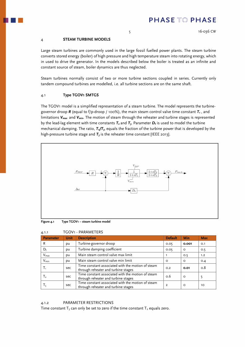
The TGOV1 model is a simplified representation of a steam turbine. The model represents the turbine-

governor droop R (equal to f/p-droop / 100%), the main steam control valve time constant T1 , and

limitations Vmax and Vmin. The motion of steam through the reheater and turbine stages is represented

by the lead-lag element with time constants T2 and T3. Parameter Dt is used to model the turbine

mechanical damping. The ratio, T2/T3, equals the fraction of the turbine power that is developed by the

high-pressure turbine stage and T3 is the reheater time constant [IEEE 2013].

Figure 4.1 Type TGOV1 – steam turbine model

4.1.1 TGOV1 - PARAMETERS

Parameter Unit Description Default Min Max

R pu Turbine-governor droop 0.05 0.001 0.1

Dt pu Turbine damping coefficient 0.05 0 0.5

Vmax pu Main steam control valve max limit 1 0.5 1.2

Vmin pu Main steam control valve min limit 0 0 0.4

T1 sec Time constant associated with the motion of steam through reheater and turbine stages

0.2 0.01 0.8


0.6 0 5


2 0 10

4.1.2 PARAMETER RESTRICTIONS

Time constant T3 can only be set to zero if the time constant T2 equals zero.

6 16-036 CW

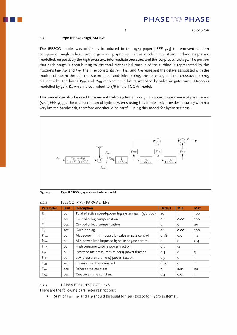
4.2 Type IEESGO 1973 SMTGS

The IEESGO model was originally introduced in the 1973 paper [IEEE1973] to represent tandem

compound, single reheat turbine governing systems. In this model three steam turbine stages are

modelled, respectively the high pressure, intermediate pressure, and the low pressure stage. The portion

that each stage is contributing to the total mechanical output of the turbine is represented by the

fractions FHP, FIP, and FLP. The time constants TCH, TRH, and TCO represent the delays associated with the

motion of steam through the steam chest and inlet piping, the reheater, and the crossover piping,

respectively. The limits Pmin and Pmax represent the limits imposed by valve or gate travel. Droop is

modelled by gain K1, which is equivalent to 1/R in the TGOV1 model.

This model can also be used to represent hydro systems through an appropriate choice of parameters

(see [IEEE1973]). The representation of hydro systems using this model only provides accuracy within a

very limited bandwidth, therefore one should be careful using this model for hydro systems.

Figure 4.2 Type IEESGO 1973 – steam turbine model

4.2.1 IEESGO 1973 - PARAMETERS


K1 pu Total effective speed-governing system gain (1/droop) 20 1 100

T1 sec Controller lag compensation 0.2 0.001 100

T2 sec Controller lead compensation 0 0 20

T3 sec Governor lag 0.1 0.001 100

Pmax pu Max power limit imposed by valve or gate control 0.98 0.5 1.2

Pmin pu Min power limit imposed by valve or gate control 0 0 0.4

FHP pu High pressure turbine power fraction 0.3 -2 1

FIP pu Intermediate pressure turbine(s) power fraction 0.4 0 3

FLP pu Low pressure turbine(s) power fraction 0.3 0 1

TCH sec Steam chest time constant 0.25 0 1

TRH sec Reheat time constant 7 0.01 20

TCO sec Crossover time constant 0.4 0.01 1


There are the following parameter restrictions:

Sum of FHP, FIP, and FLP should be equal to 1 pu (except for hydro systems).

7 16-036 CW

4.3 Type IEESGO 2003 SMTGS

The steam turbine model previously described is used in another form in the IEEE report [IEEE2013] and

presented here as IEESGO 2013. In this model three different turbine stages are represented by the

fractions K2 and K3. The relation to the IEESGO 1973 model is as follows:

𝐹𝐻𝑃 = 1 − 𝐾2

𝐹𝐿𝑃 = 𝐾2(1 − 𝐾3)

𝐹𝐿𝑃 = (𝐾2. 𝐾3)

𝑇𝐶𝐻 = 𝑇4, 𝑇𝑅𝐻 = 𝑇5, 𝑇𝐶𝑂 = 𝑇6

Figure 4.3 Type IEESGO 2013 – steam turbine model

4.3.1 IEESGO 2013 - PARAMETERS


K1 pu Total effective speed-governing system gain (1/droop) 20 1 100



T3 sec Governor lag 0.1 0.001 100



K2 pu Gain used to compute HP, IP and LP fraction 0.7 0 1

K3 pu Gain used to compute HP, IP and LP fraction 0.4 -1 1

T4 sec Low pressure turbine(s) power fraction 0.25 0.01 1

T5 sec Reheat time constant 7 0.01 20

T6 sec Steam chest time constant 0.4 0.01 1

8 16-036 CW

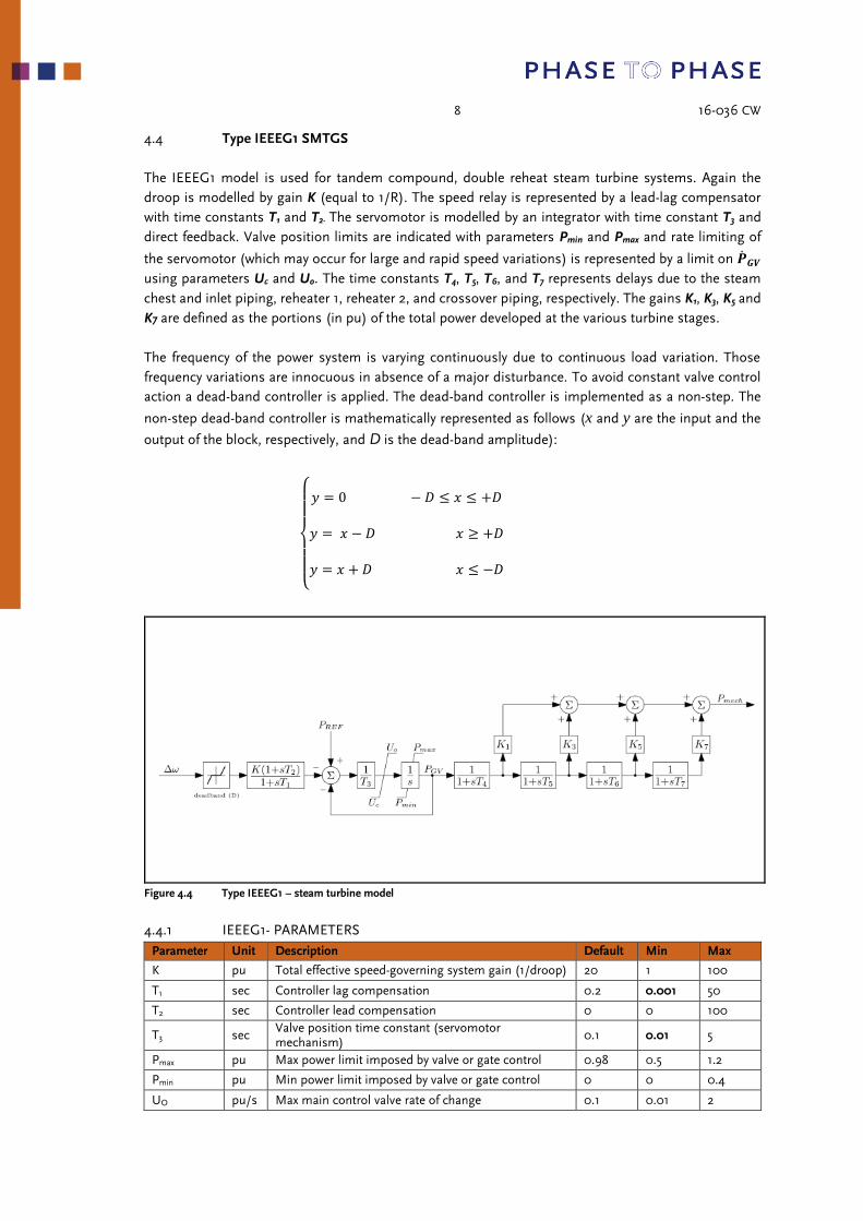
4.4 Type IEEEG1 SMTGS

The IEEEG1 model is used for tandem compound, double reheat steam turbine systems. Again the

droop is modelled by gain K (equal to 1/R). The speed relay is represented by a lead-lag compensator

with time constants T1 and T2. The servomotor is modelled by an integrator with time constant T3 and

direct feedback. Valve position limits are indicated with parameters Pmin and Pmax and rate limiting of

the servomotor (which may occur for large and rapid speed variations) is represented by a limit on 𝑮𝑽

using parameters Uc and Uo. The time constants T4, T5, T6, and T7 represents delays due to the steam

chest and inlet piping, reheater 1, reheater 2, and crossover piping, respectively. The gains K1, K3, K5 and

K7 are defined as the portions (in pu) of the total power developed at the various turbine stages.

The frequency of the power system is varying continuously due to continuous load variation. Those

frequency variations are innocuous in absence of a major disturbance. To avoid constant valve control

action a dead-band controller is applied. The dead-band controller is implemented as a non-step. The

non-step dead-band controller is mathematically represented as follows (x and y are the input and the

output of the block, respectively, and D is the dead-band amplitude):

𝑦 = 0 − 𝐷 ≤ 𝑥 ≤ +𝐷

𝑦 = 𝑥 − 𝐷 𝑥 ≥ +𝐷

𝑦 = 𝑥 + 𝐷 𝑥 ≤ −𝐷

Figure 4.4 Type IEEEG1 – steam turbine model

4.4.1 IEEEG1- PARAMETERS


K pu Total effective speed-governing system gain (1/droop) 20 1 100



T3 sec Valve position time constant (servomotor mechanism)

0.1 0.01 5



UO pu/s Max main control valve rate of change 0.1 0.01 2

9 16-036 CW

UC pu/s Min main control valve rate of change -0.1 -2 -0.01

D Hz Dead-band amplitude 0.02 0 0.06

K1 pu Fvhp, very high pressure turbine power fraction 0.22 0 1

K3 pu Fhp, high pressure turbine power fraction 0.22 0 1

K5 pu Fip, intermediate pressure turbine power fraction 0.3 0 1

K7 pu Flp, low pressure turbine power fraction 0.26 0 1

T4 sec Tch, steam chest time constant 0.25 0.01 1

T5 sec Trh1, reheat time constant 4 0.01 20

T6 sec Trh2, reheat time constant 4 0.01 20

T7 sec Tco, crossover time constant 0.4 0.01 1


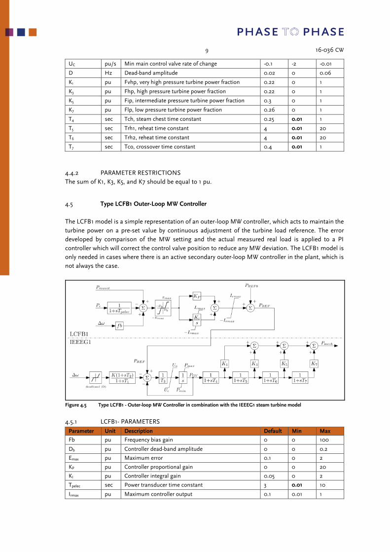
The sum of K1, K3, K5, and K7 should be equal to 1 pu. 4.5 Type LCFB1 Outer-Loop MW Controller

The LCFB1 model is a simple representation of an outer-loop MW controller, which acts to maintain the

turbine power on a pre-set value by continuous adjustment of the turbine load reference. The error

developed by comparison of the MW setting and the actual measured real load is applied to a PI

controller which will correct the control valve position to reduce any MW deviation. The LCFB1 model is

only needed in cases where there is an active secondary outer-loop MW controller in the plant, which is

not always the case.

Figure 4.5 Type LCFB1 - Outer-loop MW Controller in combination with the IEEEG1 steam turbine model

4.5.1 LCFB1- PARAMETERS


Fb pu Frequency bias gain 0 0 100

Db pu Controller dead-band amplitude 0 0 0.2

Emax pu Maximum error 0.1 0 2

KP pu Controller proportional gain 0 0 20

KI pu Controller integral gain 0.05 0 2

Tpelec sec Power transducer time constant 3 0.01 10

Irmax pu Maximum controller output 0.1 0.01 1

10 16-036 CW

5 GAS TURBINE MODELS

Currently only the GAST gas turbine model is implemented, in the near future more models (e.g. the

GGOV1 and the GT1) will be added. On request special or preferably standardised models can be

implemented.

5.1 Type GAST SMTGS

The GAST model represents the basics of a gas turbine. Parameter T1 characterizes the fuel valve

positioning time constant, the output of which is limited by Vmin and Vmax. The turbine response is

represented by a single lag time constant, T2. Turbine damping is taken into account by setting

parameter Dturb.

The temperature of the hot gasses entering the turbine need to be kept below a certain limit in order to

preserve life of the hot gas-parts of the turbine. However, it is extremely difficult to measure the gas

temperature directly. Therefore, the temperature of the exhaust is measured. Its measuring time

constant is represented by parameter T3. The ambient temperature load limit is indicated by AT and the

temperature control loop gain by KT.

Figure 5.1 Type GAST – gas turbine model

5.1.1 GAST - PARAMETERS


R pu Governor speed droop 0.05 0.001 0.1

T1 sec Governor mechanism time constant (fuel valve response)

0.1 0.01 1

T2 sec Turbine time constant 0.2 0.01 1

T3 sec Turbine exhaust temperature time constant 3 0.01 5

Vmax pu Main steam control valve max limit 1 0.5 1.2

Vmin pu Main steam control valve min limit 0 0 0.4

Dturb pu Turbine damping factor 0.3 0 1

AT pu Ambient temperature load limit 1 0 1

KT pu Temperature control loop gain 2 0 10

11 16-036 CW

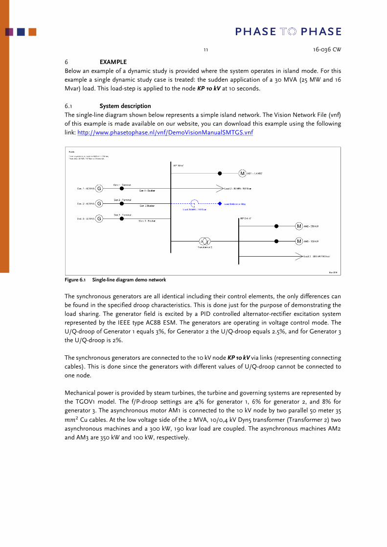
6 EXAMPLE

Below an example of a dynamic study is provided where the system operates in island mode. For this

example a single dynamic study case is treated: the sudden application of a 30 MVA (25 MW and 16

Mvar) load. This load-step is applied to the node KP 10 kV at 10 seconds.

6.1 System description

The single-line diagram shown below represents a simple island network. The Vision Network File (vnf)

of this example is made available on our website, you can download this example using the following

link: http://www.phasetophase.nl/vnf/DemoVisionManualSMTGS.vnf

Figure 6.1 Single-line diagram demo network

The synchronous generators are all identical including their control elements, the only differences can

be found in the specified droop characteristics. This is done just for the purpose of demonstrating the

load sharing. The generator field is excited by a PID controlled alternator-rectifier excitation system

represented by the IEEE type AC8B ESM. The generators are operating in voltage control mode. The

U/Q-droop of Generator 1 equals 3%, for Generator 2 the U/Q-droop equals 2.5%, and for Generator 3

the U/Q-droop is 2%.

The synchronous generators are connected to the 10 kV node KP 10 kV via links (representing connecting

cables). This is done since the generators with different values of U/Q-droop cannot be connected to

one node.

Mechanical power is provided by steam turbines, the turbine and governing systems are represented by

the TGOV1 model. The f/P-droop settings are 4% for generator 1, 6% for generator 2, and 8% for

generator 3. The asynchronous motor AM1 is connected to the 10 kV node by two parallel 50 meter 35

𝑚𝑚2 Cu cables. At the low voltage side of the 2 MVA, 10/0,4 kV Dyn5 transformer (Transformer 2) two

asynchronous machines and a 300 kW, 190 kvar load are coupled. The asynchronous machines AM2

and AM3 are 350 kW and 100 kW, respectively.

http://www.phasetophase.nl/vnf/DemoVisionManualSMTGS.vnf

12 16-036 CW

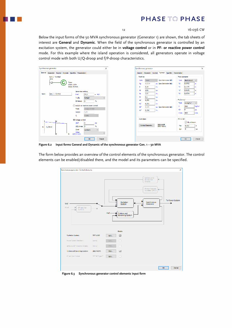
Below the input forms of the 50 MVA synchronous generator (Generator 1) are shown, the tab sheets of

interest are General and Dynamic. When the field of the synchronous generator is controlled by an

excitation system, the generator could either be in voltage control or in PF- or reactive power control

mode. For this example where the island operation is considered, all generators operate in voltage

control mode with both U/Q-droop and f/P-droop characteristics.

Figure 6.2 Input forms General and Dynamic of the synchronous generator Gen. 1 – 50 MVA

The form below provides an overview of the control elements of the synchronous generator. The control

elements can be enabled/disabled there, and the model and its parameters can be specified.

Figure 6.3 Synchronous generator control elements input form

13 16-036 CW

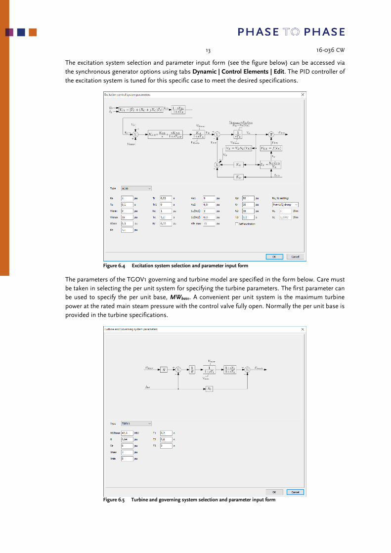
The excitation system selection and parameter input form (see the figure below) can be accessed via

the synchronous generator options using tabs Dynamic | Control Elements | Edit. The PID controller of

the excitation system is tuned for this specific case to meet the desired specifications.

Figure 6.4 Excitation system selection and parameter input form

The parameters of the TGOV1 governing and turbine model are specified in the form below. Care must

be taken in selecting the per unit system for specifying the turbine parameters. The first parameter can

be used to specify the per unit base, MWbase. A convenient per unit system is the maximum turbine

power at the rated main steam pressure with the control valve fully open. Normally the per unit base is

provided in the turbine specifications.

Figure 6.5 Turbine and governing system selection and parameter input form

14 16-036 CW

In this case the maximum turbine power is 42,5 MW, which is used as the per unit system base by the

turbine manufacturer to provide the above parameters. Hence, the synchronous machine per unit base

is Snom which is equal to 50 MVA. In the plot options all per unit variables are at the synchronous machine

base.

6.2 Dynamic study

Using this example the effect of droop control on a system operating in island mode will be illustrated.

The system is subjected to a sudden application of a 25 MW / 16 Mvar load. The response of the system,

and, in particular, the response of the generators, are to be studied in this example.

6.2.1 DYNAMIC CASE

The load-step is simulated using a workaround, since it is at this point not possible to change the system

topology during a dynamic simulation. It is however possible to apply a three phase short circuit. By

connecting a reactance coil between the node, on which the load step is to be employed, and a fictitious

node, which is used to apply the short-circuit to create a star connected load. The amplitude of both the

active- and the reactive-power step can be set by an appropriate choice of parameters R and X of the

reactor. The reactor can been seen on Figure 6.1, where it is dotted, since it is not a part of the physical

network. Below the actual dynamic event is shown, a short circuit at Node Load Reference Step.

Figure 6.6 Load step by applying a short circuit behind a reactor

To simulate a reference step of 30 MVA with a power factor of 0.85 the parameters for R and X are

determined to be 2.8574 Ω and 1.7708 Ω respectively.

15 16-036 CW

6.2.2 EXPECTED BEHAVIOUR

The initial reference active power output of the three generators equals 60 % (25.5 MW). To match the

load demand each generator will contribute based upon the user specified f/P-droop characteristic. The

system will initially be at the nominal frequency, ω0. By applying the short-circuit after the reactance coil

at 10 seconds, the system load demand increases. This increase is responsible for a decrease in both

system frequency and voltage. The governors will increase the mechanical output until they reach a new

common operating frequency, ω’. The active power output of each generator depends on the droop

characteristic, which is illustrated in Figure 6.7.

Figure 6.7 Load sharing parallel generators with drooping governor characteristics

It can been seen that Generator 1, with a f/P-droop of 4% contributes more to the load sharing than the

other two generators. From the specified f/P-droop the contributions of each generator can be

computed. They are as follows: 46.15 % (Generator 1), 30.77 % (Generator 2) and 23.08 % (Generator

3). The system will find its equilibrium at ω’ with generator outputs P1’, P2’, and P3’.

The voltage drop in response to the change in reactive power demand, will cause the AVRs to respond.

The amount of reactive load picked up by each generator depends on the U/Q-droop characteristics.

Since Generator 3 has the smallest U/Q-droop setting we can expect that this generator is going to

deliver the most reactive power. For more details on excitation systems and the U/Q-droop see:

http://www.phasetophase.nl/pdf/SynchronousMachineExcitationSystems.pdf

6.2.3 SIMULATION

A dynamic simulation can be started using Calculate | Dynamic analysis. For this example some

advanced settings are used: (1) for the initialisation of the system, where time domain initialisation is

employed, and (2) for the resistance of the short circuit, which is set to 1e-6 pu. Time domain

initialisation is used in case if a dynamic simulation does not start in steady-state. This might occur due

to the differences between models used for the loadflow and the dynamic calculation. With this

initialisation method an “empty” dynamic simulation (without selected dynamic case) is performed first.

After that, the states obtained at the specified end time (100 seconds in the example below) are used to

initialise the actual dynamic simulation (with the selected dynamic case). Below the windows with

calculation parameters are shown, the end time of the simulation of the selected dynamic case is 200

seconds.

Figure 6.8 Dynamic calculation settings

http://www.phasetophase.nl/pdf/SynchronousMachineExcitationSystems.pdf

16 16-036 CW

6.2.4 SIMULATION RESULTS

The frequency of the system in response to the load step is shown below in Figure 6.9. Since all generators

are identical, the system frequency can be obtained by observing the speed of one of the generators. The

system is initialised at the nominal frequency (50 Hz), after applying the load step the frequency stabilizes at

0.9904 pu or 49.52 Hz.

Figure 6.9 System frequency in response to a 25 MW / 16 Mvar load step

To stabilise the system the three governors will increase the turbine mechanical power output based

upon the frequency drop and the specified f/P-droop. The mechanical outputs of the three turbine

governing systems are shown below in Figure 6.10

Figure 6.10 Mechanical turbine output in MW

17 16-036 CW

The mechanical power input of Generator 1 after the application of the 30 MVA load equals 38.2 MW,

which can be validated as follows:

Δ𝑃1 =Δ𝜔

𝑅1=1.000789 − 0.99038

0.04= 0.260225 𝑝𝑢

The total turbine mechanical power output should be equal to:

𝑃1′ = 𝑃1 + Δ𝑃1

= 27.14 + (0.260225 ∗ 42.5)

= 38.2 𝑀𝑊

This corresponds to the obtained simulation results. The steam control valve position (governor output)

of the three units is plotted in Figure 6.11, where at 11.4 seconds (1.4 seconds after applying the load

step) the control valve position of Generator 1 is limited at 1 pu. This limitation can also be observed in

Figure 6.10, where the slope of the blue curve changes around 35 MW.

Figure 6.11 Steam control valve position

18 16-036 CW

Since the 30 MVA load step also includes a step of reactive power of 16 Mvar, the system terminal

voltage will drop. All generators are operating in voltage control mode with U/Q-droop characteristics.

Below the terminal RMS voltage of Generator 1 is shown in pu.

Figure 6.12 Terminal RMS per unit voltage generator 1

The influence of the U/Q-droop can be observed in the excitation system response. The droop setting

of Generator 3 is smaller than that for the other two generators and this can be directly seen in the plot

below. The contribution of Generator 3 to the reactive power demand is therefore larger than the

contribution of the other two generators.

Figure 6.13 Excitation system output voltage, EFD

19 16-036 CW

Below the actual reactive power output of the three generators is shown. The steep slopes that can be

observed at 10 seconds are the results of the computation method of the instantaneous reactive power.

Figure 6.14 Reactive power output of Generators 1, 2, and 3

In order to stabilise the perturbed system both the excitation control, and the turbine and governing

systems become active. This is a logical consequence since the dynamic case implies both a step of

active and reactive power. It is however difficult (in this example) to perform a separate analysis of

excitation and governor-turbine system behaviour. A step of the active power influences active power

balance and the system frequency, but besides that also the terminal voltage (although to a less extent).

Both controllers are acting at the same moment, which has an effect on the dynamic behaviour and the

final steady-state values of active and reactive powers of generators. To analyse those effects separately

one can easily change the dynamic case to a purely active or purely reactive load step.

7 BIBLIOGRAPHY

[IEEE1973] I. C. Report, “Dynamic Models for Steam and Hydro Turbines in Power System Studies,”

in IEEE Transactions on Power Apparatus and Systems, vol. PAS-92, no. 6, pp. 1904-1915,

Nov. 1973. doi: 10.1109/TPAS.1973.293570

[IEEE2013] I.C. Report, “Dynamic Models for Turbine-Governors in Power System Studies,” IEEE PES-

TR1, 2013.

Documents

Synchronous Machine Excitation System, Vision · PDF file162 -036 CW 3 SYNCHRONOUS MACHINE TURBINE-GOVERNING SYSTEMS The conventional primary energy sources used for electrical