Synchronization of terrestrial processes with frequencies

Astronomical and Astrophysical Transactions (AApTr), 2017, Vol. 30, Issue 2, pp. 249–260,ISSN 1055-6796, Photocopying permitted by license only, c©Cambridge Scientific Publishers

Synchronization of terrestrial processes withfrequencies of the Earth–Moon–Sun system

N.S. Sidorenkov∗

Hydrometcenter of Russia, 11–13 Bolshoi Predtechensky Pereulok, Moscow123242, Russia

Received 1 March, 2017

It is proposed that the frequencies of the quasi-biennial oscillation (QBO) of atmo-spheric winds and the Chandler wobble (CW) of the Earth’s poles are synchronizedwith each other and with the fundamental frequencies of the Earth–Moon–Sun system.The QBO and CW frequencies are resonance combinations of the frequencies of theEarth–Moon system’s yearly rotation around the Sun, precessions of the lunar orbit,and the motion of its perigee. The QBO and CW frequencies are in a ratio of 1:2.The synchronizations between Mul’tanovskii’s natural synoptic periods and tidal os-cillations of the Earth’s daily rotation rate, as well as between variations in climaticcharacteristics and long-time fluctuations of the Earth’s rotation rate are described.

Keywords: Chandler wobble, quasi-biennial oscillations of winds, cosmic effects, weatherforecast, climate change

1 Introduction

Three hundred and fifty years ago, Christian Huygens discovered the self-synchroni-zation of a pendulum clock. By now it has been established that synchronization is,according to I.I. Blekhman (1988), the property of material objects of various natureto generate a unified rhythm of joint motion despite the difference in their individ-ual rhythms and their sometimes rather weak coupling. Synchronization phenomenahave been found in acoustic and electromechanical systems, electrical circuits, radioengineering, radio physical, mechanical, and engineering devices, and living systems.

The synchronization (comparability) of the orbital and spin frequencies of planetsand moons in the solar system is widely known. By the synchronization, comparabil-ity, or resonance of a system in which the bodies rotate with orbital angular velocitiesωi, we mean linear expressions of the form

n1ω1 + n2ω2 + ..........+ nkωk = 0, (1)

where the coefficients ni are small integers.

∗Email: [email protected]

250 SIDORENKOV

2 Orbital motion of planets

To date numerous comparability relations have been found for the orbital and spinangular velocities of bodies in the solar system. Following A.M. Molchanov (1973),for illustrative purposes, we present comparability relations between the mean orbitalangular velocities of all planets in the solar system (Table 1). Here, the up-to-dateorbital periods of the planets are presented in line 1 ; the coefficients ni from expression(1) for each of the planets are given in lines 2–9; and the actual and theoretical ratios ofthe planets’ angular velocities ωi to Jupiter’s ω5, in lines 10 and 11, respectively. Thelast line (line 12) gives the relative deviations of the theoretical values ωT (calculatedusing formula (1)) from the actual values ωO. It can be seen that they are small.So, given the orbital angular velocity ωk of one planet, we can fit the values of ωi forthe other seven planets of the solar system. For example, Venus’ angular velocity ω2

is equal to the sum of Saturn’s velocity ω6 and three times Mars’ velocity ω4. Therelative error of the result is 0.2 %.

3 Earth’s monthly motion

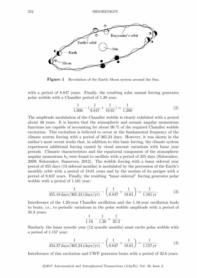
It is well known that the Earth and the Moon rotate around their center of mass(barycenter) with a sidereal period of 27.3 days. The orbit of the Earth’s centerof mass (geocenter) is geometrically similar to the Moon’s orbit, but the orbit size isroughly 1/81 as large as that of the latter. The geocenter is, on average, 4671 km awayfrom the barycenter. In the Earth’s rotationless revolution around the barycenter, allits constituent particles trace the same nonconcentric orbits and undergo the samecentrifugal accelerations as the orbit and acceleration of the geocenter (Murray andDermott, 1999, Section 4.2). The Moon attracts different particles of the Earth witha different force. The difference between the attractive and centrifugal forces actingon a particle is called the tidal force. The generation of the lunar tidal force is a majorgeophysical effect of the Earth’s monthly motion. The rotation of the Earth–Moonsystem around the Sun (Fig. 1) leads to solar tides. The total lunisolar tides varywith a period of 355 days (13 sidereal or 12 synodic months). This period is knownas the lunar or tidal year.

The plane of the Earth and Moon’s monthly orbit precesses with a period of 18.613years. Therefore, the lunar nodes precess westward around the ecliptic, completing arevolution in 18.613 years. The lunar perigee moves eastward, completing a revolutionin 8.847 years. Because of these opposite motions, a node meets a perigee in exactlyin 6 years.

4 Polar wobble

It was indicated by Sidorenkov (2009) that the Chandler period is synchronized withthe frequencies of the Earth–Moon–Sun system. The atmospheric forcing of the polarwobble with a solar year period of 365.24 days is modulated by the precession of theEarth’s monthly orbit with a period of 18.613 years and by the motion of its perigee

c©2017 Astronomical and Astrophysical Transactions (AApTr), Vol. 30, Issue 2

SYNCHRONIZATION OF TERRESTRIAL PROCESSES 251

Table

1N

ewSB

SQ

SO

candid

ate

sfo

und

by

WIS

Eco

lors

.

Pla

net

Mer

cury

Ven

us

Eart

hM

ars

Jupit

erSatu

rnU

ranus

Nep

tune

Orb

ital

per

iod

87.9

693

224.7

008

365.2

5636

686.9

796

4332.8

201

10755.6

99

30687.1

560190.0

3n1

10

00

00

00

n2

–1

10

00

00

0n3

–2

01

00

00

0n4

–1

–3

–2

10

00

0n5

00

1–6

2–2

–1

0n6

0–1

–1

0-5

50

0n7

00

1–2

00

7-1

n8

00

00

00

02

ωO/ω5

obse

rved

49.2

538

19.2

826

11.8

624

6.3

0706

10.4

0284

0.1

4119

0.0

7199

ωT/ω5

theo

ry49.2

425

19.3

240

11.7

58

6.2

824

10.4

000

0.1

4286

0.0

706

ωT−ωO

ωO

0.0

002

0.0

021

0.0

011

–0.0

039

00.0

071

0.0

117

–0.0

19

Note

:n1

ton8

are

the

coeffi

cien

tsin

Eq.

(1).


252 SIDORENKOV

Figure 1 Revolution of the Earth–Moon system around the Sun.

with a period of 8.847 years. Finally, the resulting solar annual forcing generatespolar wobble with a Chandler period of 1.20 year:

1

1.000− (

1

8.847+

1

18.61) =

1

1.200. (2)

The amplitude modulation of the Chandler wobble is clearly exhibited with a periodabout 40 years. It is known that the atmospheric and oceanic angular momentumfunctions are capable of accounting for about 90 % of the required Chandler wobbleexcitation. This excitation is believed to occur at the fundamental frequency of theclimate system forcing with a period of 365.24 days. However, it was shown in theauthor’s most recent works that, in addition to this basic forcing, the climate systemexperiences additional forcing caused by cloud amount variations with lunar yearperiods. Climatic characteristics and the equatorial component of the atmosphericangular momentum h2 were found to oscillate with a period of 355 days (Sidorenkov,2009; Sidorenkov, Sumerova, 2012). The wobble forcing with a lunar sidereal yearperiod of 355 days (13 sidereal months) is modulated by the precession of the Earth’smonthly orbit with a period of 18.61 years and by the motion of its perigee with aperiod of 8.847 years. Finally, the resulting “lunar sidereal” forcing generates polarwobble with a period of 1.161 year:

1

355.18 days/365.24 (days/yr)−(

1

8.847+

1

18.61

)=

1

1.161 yr. (3)

Interference of the 1.20-year Chandler oscillation and the 1.16-year oscillation leadsto beats, i.e., to periodic variations in the polar wobble amplitude with a period of35.3 years:

1

1.16− 1

1.20=

1

35.3.

Similarly, the lunar synodic year (12 synodic months) must excite polar wobble witha period of 1.157 year:

1

354.37 days/365.24 (days/yr)−(

1

8.847+

1

18.61

)=

1

1.157 yr. (4)

Interference of this excitation and CWP generates beats with a period of 32.6 years.



The “lunar” annual (13 anomalistic months) excitation can generate polar wobblewith a period of 1.172 year:

1

358.21 days/365.24 (days/yr)−(

1

8.847+

1

18.61

)=

1

1.172 yr. (5)

Interference of this wobble with CWP can generate beats with a period of 51.2 years:

1

1.172− 1

1.200=

1

51.17.

Thus, interference of the CW (1.20-year period) with these moon-caused oscillationsgives rise to beats, i.e., to slow periodic variations in the CW amplitude with periodsof 32 to 51 years. They are observed in reality.

Expressions (2–5) correspond to (1) with coefficients |nk| =1. They describe four-frequency synchronization or resonance. In this sense, we can say that the frequencyof Chandler polar wobble is synchronized with the fundamental frequencies of theEarth–Moon–Sun system.

5 Quasi-biennial oscillation of zonal wind

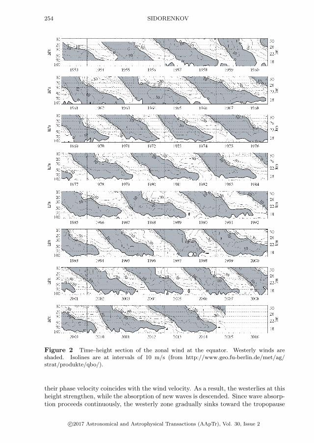
The quasi-biennial oscillation (QBO) of the atmosphere was discovered in the early1960s in the study of the equatorial stratospheric circulation. It was found that thedirection of the equatorial zonal wind reverses with a period of about 26 months inthe layer 18 to 35 km. A change from westerlies to easterlies in QBO does not happensimultaneously at all altitudes, but propagates downward at about 1 km per month.An instantaneous vertical profile of zonal wind in the layer 18–31 km has the form ofa wave with easterlies following westerlies. This wave always propagates downwardand disappears near the tropopause (at a height of ≈17 km) (Fig. 2).

At present, there is a 60-year monthly time series of mass-average zonal windvelocity u in the equatorial stratosphere (layer of 19–31 km) (Sidorenkov, 2009, TableD.2). Figure 3 shows power spectra of the pole coordinate x (top) and the QBOindices u (bottom). A surprising feature is that the spectrum of QBO indices u issimilar with a factor of 2 to that of the pole’s coordinates x and y. If the horizontal-axis scale in the spectrum of the pole’s coordinates is doubled as shown in Fig. 3,then all the details in the spectrum of QBO indices u coincide with those in thepolar motion spectrum; that is the oscillation in the polar motion is reflected as thedoubled-period QBO in the atmosphere. In the equatorial stratosphere, the durationof all the Earth’s polar motion cycles is doubled.

The QBO of the equatorial zonal wind is explained by the interaction of Kelvinwaves and mixed Rossby-gravity waves with the zonal wind in the equatorial strato-sphere (Lindzen, Holton, 1968). The nature of Kelvin and mixed Rossby-gravitywaves is not clear. In the author’s view, mixed Rossby-gravity waves are manifesta-tions of the lunar tidal waves 2Q1 (6.86 days) and σ1 (7.095 days) in the atmosphere(Sidorenkov, 2010). They account for an intense wide peak at a frequency of about0.85 (day)−1 in the spectrum of the atmospheric angular momentum (Sidorenkov,2009, see Section 6.5). It is believed that Kelvin waves propagate into the strato-sphere, where they meet a westerly shear zone and are absorbed at the height where


254 SIDORENKOV

Figure 2 Time–height section of the zonal wind at the equator. Westerly winds areshaded. Isolines are at intervals of 10 m/s (from http://www.geo.fu-berlin.de/met/ag/strat/produkte/qbo/).

their phase velocity coincides with the wind velocity. As a result, the westerlies at thisheight strengthen, while the absorption of new waves is descended. Since wave absorp-tion proceeds continuously, the westerly zone gradually sinks toward the tropopause



Figure 3 Power spectra of the pole coordinate (top) and the QBO indices (bottom). Todemonstrate the curves’ similarity, the pole’s curve was transformed as follows: T = 2T0

and, S = 30S0 + 2600, where T0 and S0 are the actual values of the periods T and spectraldensities S, respectively.

at a velocity of about 1 km/month. When the westerly zone stretches down to thetropopause, the Kelvin waves have low frequencies due to the Doppler shift, while themixed Rossby-gravity waves have high frequencies. That is why the latter propagateupward. At the height of semiannual oscillations (≈35 km), they can meet an easterlyshear zone, where they are absorbed. As a result, the easterly velocity increases andthe easterly zone descends permanently from 35 km to the tropopause, where thecycle is completed. At the same time, Kelvin wave absorption begins at the heightof semiannual oscillations and a new cycle starts. In this model, the QBO periodfor wind depends only on the intensity of atmospheric waves and on the distancebetween the equatorial tropopause and the height of semi-annual oscillations in thestratosphere.

A generalization of experimental and theoretical studies has revealed that theQBO period is a linear combination of the frequencies corresponding to the doubledperiods of the tidal year (0.972 year), precession (18.61 years), and perigee (8.847years) of the Earth monthly orbit:

1

2

(1

0.972− 1

8.847− 1

18.61

)=

1

2.32. (6)

The tidal year frequency is taken in (6) because the mechanism of QBO excitationis associated with the absorption of Kelvin and mixed Rossby-gravity waves in theequatorial stratosphere. However our observations of variations in pressure, geopo-tential height, temperature, and cloudiness anomaly fields suggest that planetaryatmospheric waves known as Rossby and Kelvin waves behave as lunar tidal wavesand have the same characteristics (Sidorenkov, 2010).


256 SIDORENKOV

The study of the equatorial angular momentum of atmospheric winds has alsoshown that their spectrum is dominated by semimonthly and quasi-weekly lunarwaves, which are treated in meteorology as Yanai waves. In 1960 C. Eckart (p.319) showed that Rossby waves are, in fact, oscillations described by Laplace’s tidalequation. Taking into account all these findings, we believe that Rossby, Kelvin, andYanai waves are visual manifestations of tidal waves in the atmosphere. From yearto year, they repeat not with a tropical year period of 365.24 days, but with a periodof 13 tropical months, which is equal to 355.16 days or 0.97 yr. It is called the tidalor lunar year.

In contrast to resonance expression (2), all the frequencies in (6) have doubled pe-riods. This means that expression (6) corresponds not to the fundamental resonance,but rather to a resonance of the n-th kind, i.e., to a subharmonic oscillation (having afrequency that is a fraction of a fundamental frequency), whose existence follows fromMandelstam and Papaleksi’s theory (Mandelstam, 1947). Thus, the quasi-biennialoscillation of zonal wind in the equatorial stratosphere is a combination oscillationdriven by three periodic processes affecting the atmosphere: (a) lunar-solar tides,(b) the precession of the Earth’s monthly orbit around the barycenter of the Earth–Moon system, and (c) the motion of the pericenter of this orbit. In the QBO case,synchronization occurs at the combination frequencies of the n-th kind.

6 Mul’tanovskii’s natural synoptic periods

The lunar–solar tides deform the Earth’s shape and change the Earth’s moment ofinertia. As a result, they have a noticeable effect on the velocity of the Earth’s dailyrotation. The tidal oscillations of the Earth’s rotation rate over any time intervalcan be calculated theoretically (Sidorenkov, 2009). For illustration, Fig. 4 shows thetidal deviations of the Earth’s daily angular velocity ν in 2016. The Earth’s rotationvelocity is characterized by the relative value (Sidorenkov, 2009)

ν =δω

Ω=ω − Ω

Ω≈ −ΠE − T

T,

where ΠE is the length of Earth’s day; T is the length of the standard (atomic) day,which is equal to 86400 s; and ω = (2 · π)/ΠE and Ω = (2 · π)/86400 rad/s are theangular velocities corresponding to the Earth’s and standard days.

It can be seen that, during a tropical month, ν undergoes two semimonthly os-cillations with maxima occurring at the maximum distance of the Moon from thecelestial equator in both Northern and Southern hemispheres (i.e., at “stations of theMoon”) and with minima occurring when the Moon intersects the equator (i.e., at“lunar equinoxes”).

The monitoring of tidal oscillations of ν, the evolution of atmospheric synopticprocesses, atmospheric circulation patterns, and time variations in hydrometeorologi-cal characteristics has shown that most types of atmospheric synoptic processes varysynchronously with the tidal oscillations of the Earth’s angular velocity (Sidorenkov,2009). Using retrospective data, we verified how frequently the extrema (minima ormaxima) of ν coincide in time with changes in elementary synoptic processes (ESP) interms of the Vangengeim classification. A statistical analysis showed that 76 % of the



Figure 4 Tidal oscillations of the Earth’s rotation velocity ν in 2016. The vertical axisrepresents the relative deviations of ν multiplied by 1010. Numerals indicate the dates whenmaxima and minima occurred.

extrema of ν coincide in time (up to 1 day) with ESP changes. In the other 24 % ofthe cases, the extrema of ν are two and more days away from the nearest ESP change(Sidorenkov, 2009). The long-time comparative monitoring of tidal oscillations of νand variations in meteorological characteristics in Moscow, Vladivostok, and othersites clearly suggests that variations in meteorological characteristics agree in timewith quasi-weekly extrema of ν (http://geoastro.ru).

Variations in weather elements at other sites of the world have been monitored byS.P. Perov and L.V. Zotov. Their results also confirm that variations in meteorologicalcharacteristics are synchronized with oscillations of the Earth’s angular velocity.

The tidal oscillations in the Earth’s rotation velocity represent a perfect index forthe features of the Earth’s monthly rotation around the barycenter and time varia-tions in the lunisolar tidal forces. They correlate with quasi-weekly and semimonthlyvariations in atmospheric processes and with local anomalies in the air temperature,pressure, cloudiness, and precipitation amounts depending on those variations.

Changes in weather patterns coincide with extrema of tidal oscillations of ν, whichcorrespond to lunar solstices and lunar equinoxes. By analogy with three-monthseasons of the year, which are associated with the Earth’s rotation around the Sun,some kind of quasi-weekly weather “seasons” can be identified in weather patterns.

Quantized weather patterns were first described by B.P. Mul’tanovskii (1933) 100years ago. He called them natural synoptic periods (NSPs). The above observationssuggest that Mul’tanovskii’s NSPs are possibly caused by the monthly rotation ofEarth and Moon around their barycenter. Weather is synchronized with the times oflunar equinoxes and solstices. In contrast to solar seasons, the lunar NSPs are notconstant: they vary from 4 to 9 days with a mean of 6.8 days. These variations arecaused by the frequency modulation of the tidal force oscillations due to the motion


258 SIDORENKOV

of the lunar perigee. Plots of tidal oscillations of ν provide a kind of NSP timetable,demonstrating that variations in NSP lengths are not random. Unfortunately, thereare still works appearing in which the dynamics of NSPs is erroneously treated interms of Brownian motion.

Note that synchronization does not determine the formation mechanisms of ther-mobaric structures due to the baroclinic instability of the atmosphere, but ratherimposes evolution rhythms close to tidal force oscillations (more precisely, to rhythmsin the Earth–Moon–Sun system) on atmospheric processes.

7 Antarctic circumpolar wave

In the Southern Ocean, large-scale anomalies of the atmospheric sea level pressure,meridional wind stress, sea surface temperature, sea surface height, and ice edge ex-tent propagate eastward around Antarctica, circling the globe every 8–10 years. Thisphenomenon was discovered by White and Peterson (1996) and Jacobs and Mitchell(1996) and was called the Antarctic Circumpolar Wave (ACW). Over the entire obser-vation span, all anomalies appear quasi-periodic with a dominant 4-year period (seeFig. 1 by White and Peterson (1996) http://circulaciongeneral.at.fcen.uba.ar/materi-al/White-Peterson.1996.pdf) and a 180 longitude wavelength.

Thus, the ACW appears as two anomalies on opposite sides of Antarctica, prop-agating eastward at about 10 cm/s. The ACW is generated by the ENSO (Turner,2004). ACW revolutions with periods of 8 and 4 years suggest that the ACW issynchronized with the frequencies of the Earth–Moon system. Indeed, the Moon’srotation involves a Full Moon Cycle (FMC) of 412 days and its subharmonic witha period of 206 days (Sidorenkov et al., 2014). The 412-day period is one of beatsgenerated by the frequencies of the synodic and anomalistic months:

1

27.5546− 1

29.5306=

1

411.793.

Three and a half FMCs take 4 years, while seven FMCs continue 8 years. There-fore, the interaction of 412- and 206-day cycles with the annual solar period (365.24day) generates beats with periods of 4 and 8 years. Accordingly, tidal geophysical,meteorological, oceanological, and other terrestrial processes exhibit 4-year cycles. Itis with these cycles of the Earth–Moon–Sun system that the ACW is synchronized.

8 Decadal climate changes

The synchronization of variations in meteorological characteristics with variations inthe Earth’s angular velocity ν and the motion of bodies in the Earth–Moon–Sunsystem can be observed not only on intramonthly time scales, but also on interannualand decadal scales.

Hot summers and cold winters over European Russia were observed in years closeto 2002/2010, 1972, 1936/1938, and 1901 (Sidorenkov, Sumerova 2012). It is close tothese years that we could observe changes in the Northern Hemisphere decadal tem-perature tendencies, atmospheric circulation epochs, the Indian monsoon intensity,



Figure 5 Synchronous changes in the Earth’s rotation velocity ν×108 (solid lines) and offive year running anomalies of the Northern Hemisphere’s air temperature after eliminationof parabolic trend (dashed lines). Original data from HadCRUT3.

the mass of the Antarctic and Greenland ice sheets, and Earth’s rotation rate regimes(Fig. 11.5) (Sidorenkov, 2009).

The renewed results presented in Fig. 5 show that the temperature T grows whenthe Earth’s rotation speeds up and decreases when the Earth’s rotation slows down.The curve of ν correlates with variations in T with correlation coefficient r = 0.67.

Singular spectrum analysis (expansion in terms of empirical orthogonal functionsof time) applied to series of the Earth’s angular velocity and global air temperatureand sea level anomalies suggests the presence of periods close to lunar periods of 18.6and 8.85 years (Zotov et al., 2014).

According to observations, the values of ν and T reached their maxima in 2003. In2004 a new epoch started in the atmospheric circulation, with Earth’s rotation rateν slowing down and T reducing.

A more detailed presentation can be found in Sidorenkov’s publications (see http://geoastro.ru), where variations in meteorological elements are compared with ex-trema of ν over the years 2012–2015.

References

Blekhman I.I. (1988) Synchronization in Science and Technology. New York, ASMEPress.


260 SIDORENKOV

Eckart, C. (1960) Hydrodynamics of Oceans and Atmospheres. New York, PergamonPress.

Jacobs G.A., J.L. Mitchell (1966) Geophys. Res. Letters, 23(21): 2947–2950.Lindzen, R.S., Holton, J.R. (1968) J. Atmos. Sci., 25: 1095–1107.Mandelstam L.I. (1947) Complete Collection of Works, USSR Acad. Sci., Moscow,

Vol. 2 (n Russian).Molchanov A.M. (1973) Modern Problems in Celestial Mechanics and Astrodynamics,

Nauka, Moscow (in Russian).Mul’tanovskii B.P. (1933) Basic Principles of the Synoptic Method for Long-Term

Weather Forecast. TsUEGMS, Moscow (in Russian).Murray, C.D., Dermott S.F. (1999) Solar System Dynamics. Cambridge University

Press. London.Sidorenkov N.S. (2009) The interaction between Earth’s rotation and geophysical

processes. Weinheim, WILEY-VCH Verlag, 317 pp.Sidorenkov N.S. (2010) Geofiz. Issled., special issue, 11: 119–128 (in Russian).Sidorenkov N.S., V.V. Chazov, and J. Wilson (2014) “On the separation of solar and

lunar cycles”, Processes in Geomedia: Collection of Scientific Papers, Moscow:IPMech RAS, pp. 118–123 (ISBN 978-5-91741-129-3).

Sidorenkov N.S., Sumerova K.A. (2012) Russian Meteorol. Hydrol., 37(6): 411–420.Turner J. (2004) Review the El Nino Southern Oscillation and Antarctica. Int. J.

Climatol., 24: 1–31.White W.B., R.G. Peterson (1996) Nature, 380: 699–702.http://circulaciongeneral.at.fcen.uba.ar/material/White-Peterson.1996.pdf.Zotov L.V., Bizouard Ch., Sidorenkov N.S. (2014) Common oscillations in global

Earth temperature, sea level, and Earth rotation, Poster at the EGU GeneralAssembly 2014: Geoph. Res. Abstr. 16. EGU2014-5683.


Documents

Synchronization of terrestrial processes with frequencies