Embed Size (px)
Citation preview

Symmetries of Quantum Mechanics
Roman Zwicky, University of Edinburgh
March 26, 2015

Contents
1 Preliminaries 11.1 Introduction . . . . . . . . . . . . . . . . . . . . . . . . . . . . . . . . . . . . . . . . . . 11.2 Basic mathematical notions . . . . . . . . . . . . . . . . . . . . . . . . . . . . . . . . . 2
1.2.1 Notation . . . . . . . . . . . . . . . . . . . . . . . . . . . . . . . . . . . . . . . . 21.2.2 Definitions . . . . . . . . . . . . . . . . . . . . . . . . . . . . . . . . . . . . . . 3
1.3 Mini-revision of linear algebra . . . . . . . . . . . . . . . . . . . . . . . . . . . . . . . . 41.3.1 Some properties of matrices . . . . . . . . . . . . . . . . . . . . . . . . . . . . . 6
2 Group theory 102.1 Basics of group theory . . . . . . . . . . . . . . . . . . . . . . . . . . . . . . . . . . . . 10
2.1.1 Group presentation . . . . . . . . . . . . . . . . . . . . . . . . . . . . . . . . . . 142.2 Notions of group theory . . . . . . . . . . . . . . . . . . . . . . . . . . . . . . . . . . . 14
2.2.1 Cosets . . . . . . . . . . . . . . . . . . . . . . . . . . . . . . . . . . . . . . . . . 142.2.2 Group action . . . . . . . . . . . . . . . . . . . . . . . . . . . . . . . . . . . . . 162.2.3 Normal subgroups . . . . . . . . . . . . . . . . . . . . . . . . . . . . . . . . . . 192.2.4 Direct and semidirect products of groups . . . . . . . . . . . . . . . . . . . . . 21
2.3 Permutation groups . . . . . . . . . . . . . . . . . . . . . . . . . . . . . . . . . . . . . 232.3.1 The symmetric permutation group Sn . . . . . . . . . . . . . . . . . . . . . . . 232.3.2 The alternating group An . . . . . . . . . . . . . . . . . . . . . . . . . . . . . . 25
2.4 Platonic solids . . . . . . . . . . . . . . . . . . . . . . . . . . . . . . . . . . . . . . . . 252.5 Applications . . . . . . . . . . . . . . . . . . . . . . . . . . . . . . . . . . . . . . . . . . 27
3 Representation theory 293.1 Representations the pedestrian way . . . . . . . . . . . . . . . . . . . . . . . . . . . . . 303.2 Basic definitions of representation theory . . . . . . . . . . . . . . . . . . . . . . . . . 303.3 Basics of representation theory Maschke’s thm, Schur’s Lemma and decomposability . 32
4 Representation theory of finite groups 344.1 Character theory for finite groups . . . . . . . . . . . . . . . . . . . . . . . . . . . . . . 344.2 Character tables . . . . . . . . . . . . . . . . . . . . . . . . . . . . . . . . . . . . . . . 38
4.2.1 Character table of S3 as an illustration . . . . . . . . . . . . . . . . . . . . . . . 414.3 Restriction to a subgroup – branching rules . . . . . . . . . . . . . . . . . . . . . . . . 43
4.3.1 Complex and real representations . . . . . . . . . . . . . . . . . . . . . . . . . . 434.3.2 Branching rules . . . . . . . . . . . . . . . . . . . . . . . . . . . . . . . . . . . . 44
i
CONTENTS ii
4.4 Constructing representations . . . . . . . . . . . . . . . . . . . . . . . . . . . . . . . . 464.4.1 A short notice on the irreducible representations of Sn . . . . . . . . . . . . . . 474.4.2 Direct product representations – Kronecker product . . . . . . . . . . . . . . . 49
4.5 A few sample applications . . . . . . . . . . . . . . . . . . . . . . . . . . . . . . . . . . 514.5.1 Distortion of lattices . . . . . . . . . . . . . . . . . . . . . . . . . . . . . . . . . 514.5.2 Fermi and bose statistics . . . . . . . . . . . . . . . . . . . . . . . . . . . . . . 51
5 Lie groups: U(1) ' SO(2), SO(3) ' SU(2)/Z2 565.1 Basic definitions . . . . . . . . . . . . . . . . . . . . . . . . . . . . . . . . . . . . . . . 565.2 The two abelian groups: U(1) and SO(2) . . . . . . . . . . . . . . . . . . . . . . . . . 605.3 Some generalities of (non-abelian) simple compact Lie groups . . . . . . . . . . . . . . 635.4 The two non abelian groups: SU(2) and SO(3) . . . . . . . . . . . . . . . . . . . . . . 66
5.4.1 Lie Algebras of SO(3) and SU(2) . . . . . . . . . . . . . . . . . . . . . . . . . . 665.4.2 Irreducible representations of SU(2) (and hence SO(3)) . . . . . . . . . . . . . 685.4.3 Clebsch-Gordan series of SU(2) . . . . . . . . . . . . . . . . . . . . . . . . . . . 71
6 Applications to quantum mechanics 746.1 A short synopsis of quantum mechanics . . . . . . . . . . . . . . . . . . . . . . . . . . 746.2 SU(2)-group theory and the physics of angular momentum . . . . . . . . . . . . . . . 776.3 Selection rules I: Wigner-Eckart theorem for SU(2) (and SO(3)) . . . . . . . . . . . . 806.4 Wigner-Eckart applied: the Lande g-factor . . . . . . . . . . . . . . . . . . . . . . . . . 846.5 Spherical harmonics . . . . . . . . . . . . . . . . . . . . . . . . . . . . . . . . . . . . . 876.6 Selection rules II: parity and superselection . . . . . . . . . . . . . . . . . . . . . . . . 906.7 Wigner-Eckart applied: electric dipole selection rules . . . . . . . . . . . . . . . . . . . 916.8 Pauli’s Hydrogen atom and SU(2)⊗ SU(2)-symmetry . . . . . . . . . . . . . . . . . . 92

Bibliography
[Arm88] M.A. Armstrong. Groups and Symmetry. Springer Verlag, New York, USA, 1988.
Undergraduate text on groups theory with focus in finite groups.
[Ful91] W.Fulton and J.Harris Representation theory - A first course. Springer Verlag, Graduate textin mathematics, New York, USA, 1991.
Graduate text. More advanced. Pedagogical text, especially beginning of the book has a nicediscussion on representation theory of finite groups. For the student who wants to know more.
[Gil08] R.Gilmore Lie Groups, Physics, and Geometry: An Introduction for Physicists, Engineersand Chemists. Cambdridge University Press 2008
An inspiring book with lots of good examples.
[Tun85] Wu-Ki Tung. Group theory in physics. World Scientific, Singapore, 1985.
A widely used textbook for the subject.
[Atk08] Peter Atkins and Julio de Paula Atkins’ Physics Chemistry. Oxford University Press, ninthedition , 2010
Efficient use of group theory.
[Ham62] Morton Hammermesh Group Theory and its Application to Physical Problems. Dover Pub-lications Inc. New York, 1962
A readable classic on the subject.
[Corn97] J.F. Cornwell Group Theory in Physics. Academic Press, 1997
A widely used textbook.
[Ell79] J.P.Elliott and P.G.Dawber Symmetry in Physics. MacMillan press LTD, 1979
Very well known among particle physicists.
[Geo99] H.Georgi Lie Algebras in Particle Physics. Frontiers in Physics 2nd ed, 1999
Idem.
[Gre97] W.Greiner and B.Muller Quantum Mechanics: Symmetries Greiner’s book are usually ap-preciated for their explicitly working out many examples. Springer 1997

Chapter 1
Preliminaries
1.1 Introduction
The theory of finite groups has historically arisen as an effort (by Galois) to classify different solutionsof algebraic equations. The theory of Lie Groups was founded by Lie in an attempt to classify solutionsof differential equations. Lie groups turned out to be continuous groups with a natural manifoldstructure. Both types will be discussed in this course.
Generally group theory is a standard algebraic structure which applies in many fields of mathe-matics and applied sciences. In physics, symmetries are naturally described by groups. The powerof symmetries relies on the fact that they, partially, solve the dynamics; the symmetry restricts thesolutions. This happens at the more sophisticated level of the celebrated Wigner-Eckart theorem (tobe discussed in these lectures) as well as in simple integrals where the symmetries of the integrandrestrict the form of the solutions.
An example is the following integral
Iij =
∫d3kf(k · p, k2, p2)kikj = A(p2)δij +B(p2)pipj , (1.1)
where ki, pi are vectors in three dimensional space and δij is the Kronecker symbol. The integral of atype Iij is an integral that describes quantum correction, be it in quantum field theory or statisticalmechanics. No matter how complicated the function f is, the solution has the form on the right handside since the integrand is covariant under the three dimensional euclidian rotation group. If thesymmetry is not assumed then one ought to write 3 · 3 = 9 coefficients instead of the two coefficientsA and B above.
At the level of equations of motion, or more precisely the Lagrangian, symmetries are relatedto conservation laws by virtue of the famous Noether theorem. Most famously: time symmetry⇔ energy conservation, space translation symmetry ⇔ momentum conservation, rotational symmetry⇔ spatial angular momentum conservation. The result can often be turned around in the sense that anunexpected symmetry in the result suggests that a symmetry in the Lagrangian has been overlooked.
Groups are abstract objects in principle. When realised on vector spaces they are referred toas representations. As quantum theory is described by Hilbert spaces which are specific, at times
1

CHAPTER 1. PRELIMINARIES 2
infinite dimensional, vector spaces representation theory plays a special role.1 An example, that youshould have seen in a course on quantum mechanics, is the Hydrogen atom for which the potentialV ∼ 1/r has spherical symmetry (symmetry under the rotation group). The energy solutions aregiven by En ∼ 1/n2 which are in particular independent of the so-called third quantum numbers m(z-projection of the angular momentum) which singles out a direction in the physical space. Once anexternal magnetic field (an example of hyperfine splitting) is applied to the hydrogen atom, a directionis singled out. In this case, as expected, the energy depends on the magnetic quantum number m.
The course consists essentially of four parts.2 An introduction into abstract group theory withfocus on finite groups in chapter 2, generic remarks on representation theory 3, representation theoryof finite groups and of continuous groups in chapters 4 and 5 respectively followed by applicationsto quantum mechanics in chapter 6. On the subject of continuous groups special focus is given onU(1) (the symmetry group of quantum electrodynamics which is associated with charge conservation),SO(3) (the rotation group) and SU(2) (the rotation group of half integer spin objects e.g. the electronif spin 1/2).
Proofs are usually given or at least sketched. The proofs aim to give you insight about thetheorems. More elaborate proofs which give only limited insight are not given but can looked up intextbooks on group theory. Throughout the text there are plenty of footnotes. Almost all of themcould be omitted but they, hopefully, provide the reader with more insight on alternative views or abroader scope on the topic. In my personal experience this leads to higher appreciation of the topicin general. Comments on possible applications in physics, of the underlying mathematical topic, aregiven in italics. Please do not hesitate to give me comments on these notes either in person or viae-mail. Your effort is much appreciated, also by future students attending this course.
1.2 Basic mathematical notions
The aim of this section is to introduce the basic notions of mathematics used throughout the text.
1.2.1 Notation
Basic notation used throughout the course:
- The integer numbers Z ≡ ..,−2,−1, 0, 1, 2, ..
- The rational numbers Q ≡ p/q | p, q ∈ Z
- The unit circle in n+ 1 dimensions is denoted by Sn = ~x ∈ Rn+1 | x21 + x2
2 + ..+ x2n+1 = 1.
- Mn(F ) corresponds to the n × n-matrices over the set F which is most often R or C in thiscourse. In denotes the unit n× n matrix.
- GL(n,C) = A ∈ Mn(C) | det(A) 6= 0 sometimes also denoted by GL(V ) where dim(V ) = nis an n-dimensional vector space.
1Also for mathematics according to this quote: “all of mathematics is a form a representation theory ” (IsraelGelfand (1913-2009)).
2The section on basic mathematical notions 1.2 will only be briefly discussed and mainly serves the purpose ofhaving a common language. The basic revision of linear algebra will be discussed before starting with the chapter onrepresentation theory 3 where it is really needed. Abstract group theory as presented in chapter 2 is independent oflinear algebra.
CHAPTER 1. PRELIMINARIES 3
- Einstein summation convention: when two identical indices (on the same side of the equation)are left ”open”, then they are meant to be summed over unless otherwise stated. For examplex∗i yi →
∑i x∗i yi.
1.2.2 Definitions
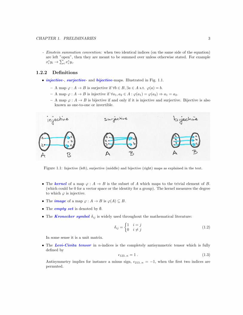
• injective-, surjective- and bijective-maps. Illustrated in Fig. 1.1.
– A map ϕ : A→ B is surjective if ∀b ∈ B, ∃a ∈ A s.t. ϕ(a) = b.
– A map ϕ : A→ B is injective if ∀a1, a2 ∈ A : ϕ(a1) = ϕ(a2)⇒ a1 = a2.
– A map ϕ : A → B is bijective if and only if it is injective and surjective. Bijective is alsoknown as one-to-one or invertible.
Figure 1.1: Injective (left), surjective (middle) and bijective (right) maps as explained in the text.
• The kernel of a map ϕ : A → B is the subset of A which maps to the trivial element of B.(which could be 0 for a vector space or the identity for a group). The kernel measures the degreeto which ϕ is injective.
• The image of a map ϕ : A→ B is ϕ(A) ⊆ B.
• The empty set is denoted by ∅.
• The Kronecker symbol δij is widely used throughout the mathematical literature:
δij =
1 i = j0 i 6= j
(1.2)
In some sense it is a unit matrix.
• The Levi-Civita tensor in n-indices is the completely antisymmetric tensor which is fullydefined by
ε123..n = 1 . (1.3)
Antisymmetry implies for instance a minus sign, ε213..n = −1, when the first two indices arepermuted.

CHAPTER 1. PRELIMINARIES 4
• An equivalence relation : is a relation between two elements, say a and b denoted by a ∼ bwhich satisfies the following three properties
1. a ∼ a (reflexivity)
2. a ∼ b implies b ∼ a (symmetry)
3. a ∼ b and b ∼ c implies a ∼ c (transitivity)
The equivalence class of an element, say a, is the set of all elements which are equivalent toa. It is denoted by [a] = x | a ∼ x. Any element of [a] is said to be a representative of theequivalence class. An example for an equivalence relation is: two vectors being parallel.
1.3 Mini-revision of linear algebra
In this section we revise some notions from linear algebra which are particularly useful for the course.
• Vector space is a collection of elements (vectors) which add and are multiplied with objects ofa field. A field is an algebraic body with certain properties. For the purpose of the course it issufficient to think of the field either as the real numbers or the complex numbers. Let ~u, ~v and~w be such vectors (think of them as vectors in Cn for example) and k and k′ complex numbersthen the following properties define a vector space:
(1) (~u+ v) + ~w = ~u+ (~v + ~w) , (5) k(~u+ ~v) = k~u+ k~v ,
(2) (~u+ 0) = ~u , (6) (k + k′)~u = k~u+ k′~u ,
(3) ~u+ (−~u) = 0 , (7) (kk′)~u = k(k′~u) ,
(4) ~u+ ~v = ~v + ~u , (8) 1~u = ~u . (1.4)
In particular the collection of vectors has a neutral element 0 (axiom (2)) and the field has aunit operators 1 (axiom (8)).
• Hilbert space is a vector space (see above) with a scalar or inner product, denoted here by (, ),from V × V → C which satisfies the following axioms:
(1) (~u, k~v + k′ ~w) = k(~u,~v) + k′(~u, ~w) , linearity ,
(2) (~u,~v) = (~v, ~u)∗ , conjugation ,
(3) (~u, ~u) ≥ 0 , positivity , (1.5)
where the equality (3) holds ⇔ ~u = 0. As an example we mention the vector space Cn over Cwith scalar product: (~u,~v) =
∑ni=1 u
∗i vi.
We ought to mention the bra and ket notation (introduced by P.A.M. Dirac and widely usedin physics) which amounts to the notational identification,
u↔ |u〉 , (u, v)↔ 〈u|v〉 , (1.6)
which we shall use at times when illustrating examples.

CHAPTER 1. PRELIMINARIES 5
• A linear operator is an operator which is compatible with linearity:
A(k|u〉+ k′|v〉) = kA|u〉+ k′A|v〉 . (1.7)
In a finite dimensional vector space all linear operators can be represented by matrices. Thiswill be of importance when discussing finite representation theory.
In order to illustrate the remaining notations we will consider a finite dimensional complex vectorspace, denoted by V = CN where N = dimV . Then there are N linearly independent vectors|ε1〉, |ε2〉, ..., |εN 〉3 which form a basis in the sense that each |v〉 ∈ V can be written as
|v〉 =
N∑i=1
vi|εi〉 , vi ∈ C . (1.8)
The inner product (, ) : V × V → C is written in the Dirac notation as follows: 〈v|w〉 ≡ (|v〉, |w〉).The combination of a vector space and an inner product are also known as a Hilbert space.4 A basis|e1〉, |e2〉, ..., |eN 〉 orthonormal to the inner product can be chosen:
〈ei|ej〉 = δij . (1.9)
The scalar product of two vectors |v〉 =∑Ni=1 vi|ei〉 and |w〉 =
∑Ni=1 wi|ei〉 is given by:
〈v|w〉 =
N∑i=1
v∗iwi . (1.10)
An orthonormal set provides a decomposition of the identity
1N =
N∑i=1
|ei〉〈ei| . (1.11)
A partition of the identity is a collection of projectors Pj ≡∑Nji=1 |ei〉〈ei| satisfying:
PiPj = δijPi , P †j = Pj , 1N =
NP∑j=1
Pj . (1.12)
Note: N =∑NPj=1Nj . A linear operator A : V → V (A(a|v〉+ b|w〉) = a(A|v〉)+ b(B|w〉) for a, b ∈ C)5
can be represented as a matrix 6 and its matrix elements are given by
Aij = 〈ei|Aej〉 ≡ 〈ei|A|ej〉 , (1.13)
3We shall use Dirac’s bra and ket notation throughout this section.4Subtleties arise in the case of infinite dimensional vector spaces which are beyond the scope of this course.5An operator is anti-linear if A(a|v〉+ b|w〉) = a∗(A|v〉) + b∗(B|w〉). The operator that changes t→ −t, denoted by
T (with t being the time), is an example of an anti-linear operator.6In this section matrix stands for a square matrix.
CHAPTER 1. PRELIMINARIES 6
where the notation on the right hand side is the one used in quantum mechanics (it is understoodthat A acts on the right i.e. |ej〉). Hence a matrix A may be written as:
A =
N∑i,j=1
Aij |ei〉〈ej | . (1.14)
A fundamental fact is that the eigenvalue equation:
A|vi〉 = λi|vi〉 , (1.15)
admits N solutions since the characteristic polynomial P (t) = det(A− t1) = 0 admits N solutions byvirtue of the fundamental theorem of algebra. The λi are said to be eigenvalues and the |vi〉 are thecorresponding eigenvectors.
1.3.1 Some properties of matrices
• The transpose of a matrix is (AT )ij = Aji. A matrix is (anti)symmetric ⇔ AT = ±A (withsymmetric for plus sign).
• The hermitian conjugate of a matrix is (A†)ij = A∗ji. A matrix is hermitian ⇔ A† = A.
• The inverse of a matrix A−1 is a matrix that satisfies: A−1A = AA−1 = 1N .
• A unitary matrix is a matrix whose hermitian conjugate is its inverse A† = A−1 ⇔ AA† =A†A = 1N .
• The trace of matrix is Tr[A] =∑〈ei|A|ei〉 where |ei〉 is an orthonormal basis.
• The determinant of a matrix is detA = εi1....iNA1i1 ....ANiN where summation over the indicesix is implied and ε123..N = 1 is the completely antisymmetric Levi-Civita tensor. The definition,which is not as simple as other definitions in this list, is given for completeness only. You shouldbe familiar with its basic properties given in section 1.3.1.
• A matrix is diagonal ⇔ Aij = 0 for i 6= j.
• A matrix A is block diagonal if it can be written as:
A =
(A1 0m×n
0n×m A2
)(1.16)
where A1 and A2 are n × n and m ×m matrices. The symbol 0i×j stands for a i × j matrixwith entries equal to zero.
• The direct sum of two vector spaces V ⊕W has the following meaning: To each |vi〉 ∈ V and|wa〉 ∈W we associate a state |vi〉⊕|wa〉 ≡ |vi⊕wa〉 (the last equality is non-standard notation)and the inner product is extended to:
〈vi ⊕ wa|vj ⊕ wb〉V⊕W = 〈vi|vj〉V + 〈wa|wb〉W (1.17)

CHAPTER 1. PRELIMINARIES 7
The dimension is dim(V ⊕W ) = v + w (v ≡ dim(V ) and w ≡ dim(W )) Given A ∈ GL(V ) andB ∈ GL(W ) then
(A⊕B)|vi〉 ⊕ |wa〉 = (A|vi〉)⊕ (B|wa〉) . (1.18)
Hence the direct sum may be thought of as a v + w-dimensional vector space where operatorsare represented as (v + w)× (v + w) matrices in block diagonal form:
A⊕B =
(A 0v×w
0w×v B
)(1.19)
The inverse problem, can a vector space be written as a direct sum, plays an important role indiscussing the irreducibility of a representation.
• The direct product of two vector spaces V ⊗W has the following meaning: To each |vi〉 ∈ Vand |wa〉 ∈W we associate a state a state |vi〉⊗|wa〉 ≡ |vi⊗wa〉 (the last equality is non-standardnotation) and the inner product is extended to:
〈vi ⊗ wa|vj ⊗ wb〉V⊗W = 〈vi|vj〉V · 〈wa|wb〉W (1.20)
The dimension is dim(V ⊗ W ) = v · w. The direct product of the two operators from theproceeding item acts on the space as follows:
(A⊗B)|vi〉 ⊗ |wa〉 = A|vi〉 ⊗B|wa〉 . (1.21)
An example in quantum mechanics is the spatial wave function of the electron Ψ(x) times (⊗)its spin 1/2 part. Direct products play a role in representation theory in terms of, what we shallcall, Kronecker products. They are widely used in physics. For example by taking Kroneckerproducts (tensor products of representations to be defined throughout the course) the so-calledfundamental representations all other representations of the group can be obtained.
Properties associated with definitions above:
1. For a hermitian matrix the eigenvalues are real (λi ∈ R) and the eigenvectors can be chosen tobe orthonormal. In this basis the matrix A is diagonal. For a two 2× 2 hermitian matrix in theorthonormal eigenbasis reads:
A =
(λ1 00 λ2
)≡ diag(λ1, λ2) , (1.22)
with obvious generalisation to n× n-matrices.
It is straightforward to construct the explicit transformation matrix. Suppose A is a hermitianand a non-diagonal matrix and λi and |vi〉 are its orthonormal eigenvectors, then
A =
N∑l=1
λl|vl〉〈vl| (1.23)

CHAPTER 1. PRELIMINARIES 8
is diagonalised by the following unitary basis transformation7
diag(λ1, ..., λN ) = V †AV , V =
N∑l=1
|vl〉〈el| . (1.24)
2. The inverse of a matrix A exists ⇔ A has no zero eigenvalues. For a hermitian matrix, theinverse in the orthonormal eigenbasis reads:
A−1 =
(λ−1
1 00 λ−1
2
). (1.25)
3. The trace of a matrix is the sum of its eigenvalues Tr[A] =∑Ni=1 λi.
4. The trace is cyclic Tr[AB] = Tr[BA].8
5. The determinant of a matrix is the product of its eigenvalues det(A) =∏Ni=1 λi.
6. The determinant of a product of matrices is the product of its determinants.
det(AB) = det(A) · det(B)(= det(BA)) . (1.26)
7. The following relation holds:〈v|Aw〉 = 〈A†v|w〉 (1.27)
This implies that for a unitary matrix U :
〈Uv|Uw〉 = 〈v|w〉 . (1.28)
Hence unitary transformations are the natural objects to implement symmetry transformationson Hilbert spaces since they preserve the inner product (probability measure).
Exercise 1.3.1 Basic linear algebra:
a) Make sure you understand all the definitions in the list given in this section and that theproperties 1) to 7) are familiar to you.
b) Show that SL(V ) = A ∈ GL(V ) | det(A) = 1 is a group. The letter “S” stands forspecial since SL(V ) is a special linear group.
c) Verify that the determinant is a group homomorphism: det : GL(V )→ C∗.
7In the case where A is not hermitian it can happen that the eigenvectors, because of linear dependence, cannot bebrought into a orthonormal form. In such cases a so-called Jordan normal form can be obtained with eigenvalues onthe diagonal and entries equal to one for A(i+1)(i−1)-elements on subspaces of degenerate eigenvalues. For more detailsconsider textbooks as this topic is beyond the scope of this course.
8The trace is also linear and 〈A|B〉 = Tr[A†B] is an inner product on the vector space of matrices.

CHAPTER 1. PRELIMINARIES 9
d) Show that〈v|Aw〉∗ = 〈w|A†v〉 . (1.29)
e) As additional exercises you might want to show that:
– det(A−1) = det(A)−1, det(aA) = aN det(A) where a ∈ C.
– Tr[AT ] = Tr[A], Tr[An] =∑Ni=1 λ
ni .
– The trace and the determinant are invariants under similarity transformations.
– Properties of hermitian conjugation (aA)† = a∗A† for a ∈ C, (A + B)† = A† + B†,(AB)† = B†A†, (A†)† = A, (a|α〉〈β|)† = a∗|β〉〈α|.

Chapter 2
Group theory
This chapter aims to familiarise the student with the basic notions of group theory. This part resemblesan undergraduate course on group theory in algebra except that the proofs are not as detailed andthat comments on applications in physics are inserted here and there. Most proofs are straightforwardfrom the viewpoint of the mathematician. The exceptions are Cauchy’s theorem and the theorem onthe alternating groups. In those cases previous results (isomorphism and orbit-stabiliser theorem)give rise to more elegant proofs.
2.1 Basics of group theory
Let us start from the formal definition of a group .
Definition 2.1.1 Group:
Let G be a set on which a binary operation G×G→ G is defined. G is called a group if and only if
(g1 · g2) · g3 = g1 · (g2 · g3) ∀g1, g2, g3 ∈ G , product rule is associative
e · g = g · e = g , ∃e ∈ G : ∀g ∈ G , there is an identity element in G.
g · g−1 = g−1 · g = e , ∀g ∈ G,∃g−1 ∈ G , every element of G has an inverse in G.
Exercise 2.1.1 To be discussed in the workshop
a) Show that (a · b)−1 = b−1 · a−1.
Examples 2.1.1 (basic ones)
- The integers Z form a group with respect to the binary operation of addition, denoted by (Z,+).The unit element is given by 0. The inverse of n is −n.
10

CHAPTER 2. GROUP THEORY 11
- The integers Z are not a group with respect to the binary operation of multiplication. First the0 element 0 · Z = 0 does not comply with the group axioms. Taking Z∗ ≡ Z\0 is not a groupeither since the inverse of say 2, which is 1/2, is not contained in the set.
- The rational numbers Q∗ (with notation understood as above), the real numbers R∗ or thecomplex numbers C∗ form a group with respect to the binary operation of multiplication, whichwe denote by (Q∗, ·) and so on.
- The group of permutation of n elements, denoted by Sn, forms a group.1 The permutationgroups will be discussed in a separate section 2.3.
- The group Zn (cyclic group of order n) with n elements e2πi(m/n) (0 ≤ m < n integer) forms agroup under multiplication.
- The rotation group of three dimensional space O(3) = O ∈M3(R) | OTO = I3. More preciselythis corresponds to the so-called fundamental representation of O(3). This viewpoint will bediscussed at length in chapter 3 on representation theory.
The examples are concrete examples of structures that you might already have known. Below wegive a few basic definitions that help to characterise a group. This can be helpful for example asspecific statements, e.g. theorems, might only be valid for certain classes of groups.
Definition 2.1.2 Basic defintions:
• A group is called finite , discrete or continuous depending on whether the set G is finite,discrete (isomorphic to Z) or uncountable.
• The order of a group G (denoted by |G|) is the number of elements of the group. Thus theorder of a group is a sensible concept for a finite group.
• The order of a group element g ∈ G is the smallest integer n for which gn = e.
• A group G is called abelian ⇔ ∀g1, g2 ∈ G : g1 · g2 = g2 · g1.2 The elements g1 and g2 aresaid to commute with each other.
• A group H is called subgroup of G (denoted by H ⊂ G) ⇔ H is a group and its elements area subset of the elements of G. A proper subgroup is a subgroup which is not the group itselfnor the group with one element (often called the trivial subgroup).
• Two elements g1, g2 ∈ G are conjugate to each other ⇔ ∃g ∈ G s.t. g1 = g · g2 · g−1.
• The generators of a group are a set of elements from which all other elements can be generatedthrough the group multiplication law. A set of generators is not unique in general. In particularthe number of elements of a generating set might differ. The minimal number of elements thatgenerate a certain group is called the rank of a group.3 It is a fact that all groups which are ofrank 1 are isomorphic to the cyclic group Zn mentioned above.
1You may think of rearranging n objects with different colours which are placed on one line. The group conceptseems very natural for investigating this object.
2In honour of the Norwegian mathematician Niels Henrik Abel (1802-1829).3For Lie groups this notion is extended to the Lie Algebra which is often finite dimensional unlike the group itself.

CHAPTER 2. GROUP THEORY 12
• The center of a group is the subset of elements which commute with all elements of the group:Z(G) = z ∈ G | ∀g ∈ G : z · g = g · z
Exercise 2.1.2 To be discussed in the workshop
a) Which groups in examples 2.1 are finite, discrete or continuous?
b) Give an element in O(3) (c.f. example 2.1 last one) which is of order 2. That is to say writedown a 3× 3 matrix in O(3), other than the identity, which squares to one.
c) Give one example of a proper and continuous subgroup of O(3). Give an example of aproper subgroup of Z4.
d) Give all minimal set of generators of Z4 and Z7 using the representation e2πi(n/4) ande2πi(n/7)
e) Show that conjugation within a group forms an equivalence relation. This fact will becomeparticularly important when discussing the representation theory of finite groups.
f) Show that for a group where each element, except the identity, is of order 2 is abelian.
Theorem 2.1.1 subgroup criteriaA subset H of a group G is a subgroup ⇔ g1 · g−1
2 ∈ H for g1, g2 ∈ H.
The proof of theorem 2.1.1 does not provide any insight and so we shall skip it.Finite groups can be represented in terms of so-called multiplication tables which simply list
all possible multiplications of the groups in terms of a rows and columns system.
G e a b ..e e a b ..a a a2 a · b .... .. .. ..
(2.1)
Examples of the cyclic group Z2 and the permutation group S3 are given in tables 2.1 and 2.2respectively. The multiplications are such that column multiplies the row which is relevant in the casewhere the two elements do not commute. One may therefore envisage the program of writing down allmultiplication tables at any finite order and verify that the result satisfies the group axioms. Whereasin principle possible you might guess that this is not the most efficient nor elegant way to characterisegroups. In essence this amounts to finding the subset of permutations which is compatible with thegroup axioms. In addition in each row and column one find each elements exactly once as otherwisethe inverse would not be unique. For example in the table if a2 = a · b then by the uniqueness of theinverse of a we would conclude a = b which is clearly wrong. This simple fact is sometimes referredto as the rearrangement theorem throughout the literature. This insight makes the following theoremobvious:
Theorem 2.1.2 Cayley’s thm:Any finite group is isomorphic (to be defined below) to a subgroup of the symmetric group Sn.
CHAPTER 2. GROUP THEORY 13
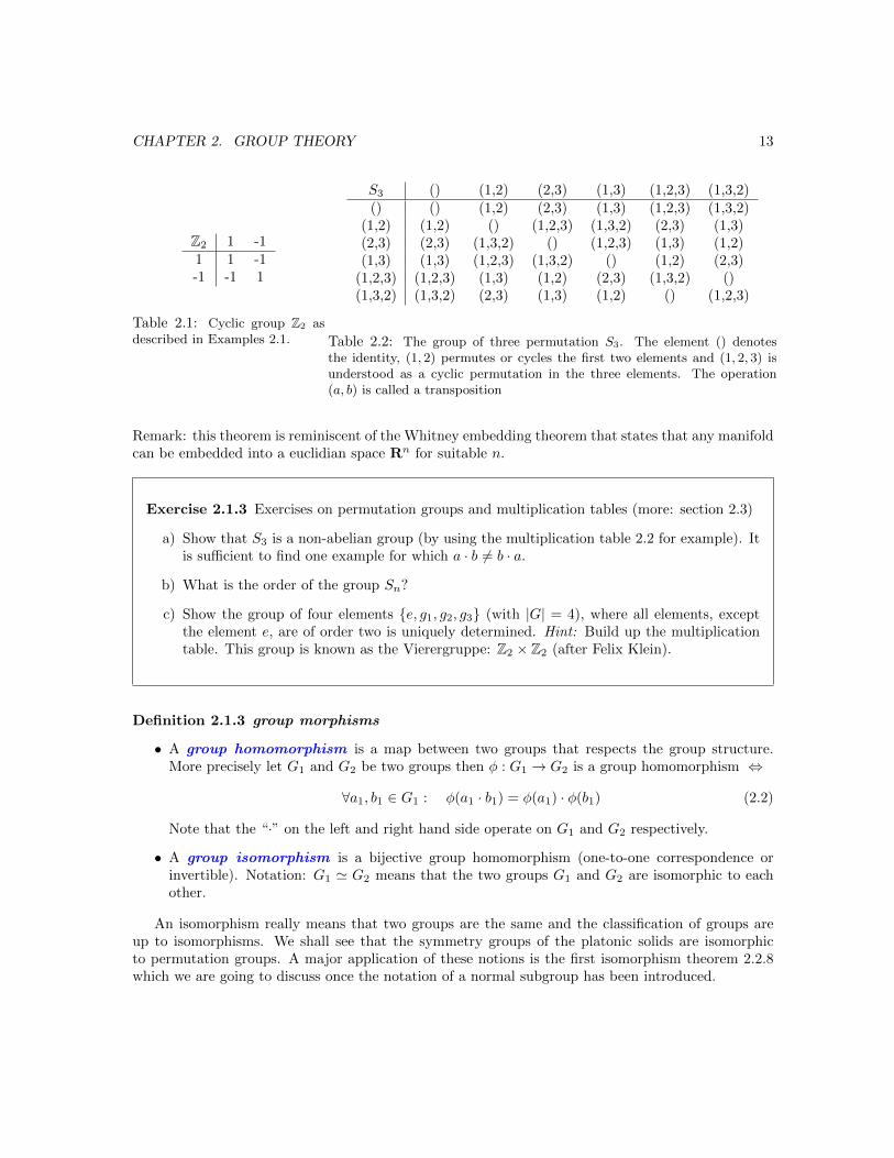
Z2 1 -11 1 -1-1 -1 1
Table 2.1: Cyclic group Z2 asdescribed in Examples 2.1.
S3 () (1,2) (2,3) (1,3) (1,2,3) (1,3,2)() () (1,2) (2,3) (1,3) (1,2,3) (1,3,2)
(1,2) (1,2) () (1,2,3) (1,3,2) (2,3) (1,3)(2,3) (2,3) (1,3,2) () (1,2,3) (1,3) (1,2)(1,3) (1,3) (1,2,3) (1,3,2) () (1,2) (2,3)
(1,2,3) (1,2,3) (1,3) (1,2) (2,3) (1,3,2) ()(1,3,2) (1,3,2) (2,3) (1,3) (1,2) () (1,2,3)
Table 2.2: The group of three permutation S3. The element () denotesthe identity, (1, 2) permutes or cycles the first two elements and (1, 2, 3) isunderstood as a cyclic permutation in the three elements. The operation(a, b) is called a transposition
Remark: this theorem is reminiscent of the Whitney embedding theorem that states that any manifoldcan be embedded into a euclidian space Rn for suitable n.
Exercise 2.1.3 Exercises on permutation groups and multiplication tables (more: section 2.3)
a) Show that S3 is a non-abelian group (by using the multiplication table 2.2 for example). Itis sufficient to find one example for which a · b 6= b · a.
b) What is the order of the group Sn?
c) Show the group of four elements e, g1, g2, g3 (with |G| = 4), where all elements, exceptthe element e, are of order two is uniquely determined. Hint: Build up the multiplicationtable. This group is known as the Vierergruppe: Z2 × Z2 (after Felix Klein).
Definition 2.1.3 group morphisms
• A group homomorphism is a map between two groups that respects the group structure.More precisely let G1 and G2 be two groups then φ : G1 → G2 is a group homomorphism ⇔
∀a1, b1 ∈ G1 : φ(a1 · b1) = φ(a1) · φ(b1) (2.2)
Note that the “·” on the left and right hand side operate on G1 and G2 respectively.
• A group isomorphism is a bijective group homomorphism (one-to-one correspondence orinvertible). Notation: G1 ' G2 means that the two groups G1 and G2 are isomorphic to eachother.
An isomorphism really means that two groups are the same and the classification of groups areup to isomorphisms. We shall see that the symmetry groups of the platonic solids are isomorphicto permutation groups. A major application of these notions is the first isomorphism theorem 2.2.8which we are going to discuss once the notation of a normal subgroup has been introduced.

CHAPTER 2. GROUP THEORY 14
Exercise 2.1.4 To be discussed in the workshop
a) Two finite groups which admit an isomorphism, obviously, have the same number of ele-ments. For continuous groups the issue is more subtle as is often the case. Can you give anisomorphism between the integer number Z and the even integers 2Z?
b) Show that for g ∈ G, g → g−1 (inversion) defines an isomorphism ⇔ G is abelian.
2.1.1 Group presentation
One may define groups from generators and their relation in a completely algebraic way. Moreprecisely consider a set of generators a, b, c, .., then the group is defined as all words (arrangementof letters) that can be formed modulo certain constraints e.g. a2 = e, b3 = e, abc = e, ... This wayof defining a group is called the group presentation . The presentation, for a given group, is notunique. For example S3 can be defined as:
S3 = < a, b, c | a2 = b2 = c3 = abc = e > (2.3)
orS3 = < A,B | A2 = B2 = (AB)3 = e > (2.4)
Presentations, at least for finite groups, will not play a major part in this course. Yet it seems goodpractice to do the following exercise:
Exercise 2.1.5 To be discussed in the workshop
a) Identify candidates for generators a, b, c and A,B in Eqs. (2.3) and (2.4) (by using themultiplication table 2.2) respectively.
2.2 Notions of group theory
2.2.1 Cosets
Definition 2.2.1 (left)-coset:Given a subgroup H ⊂ G one can associate to each g ∈ G a left-coset gH = g · h | h ∈ H
Remarks and properties:
• one can define in completely analogous manner a right-coset . Below we shall continue toreference left cosets only.

CHAPTER 2. GROUP THEORY 15
• Only for a certain subclass of groups, called normal (to be defined), one can define a groupmultiplication on cosets. Hence cosets do in general not admit a group structure and aretherefore called cosets rather than “cogroups”.
Definition 2.2.2 partitionA partition of a set is a decomposition into (non-empty) subsets which do not intersect. In terms of
symbols: Pi ⊂ X form a partition of X if X = P1 ∪ P2 ∪ .. and Pi ∩ Pj = ∅ for i 6= j.
Theorem 2.2.1 (a) The left- gH and also the right-cosets Hg partition G. (b) the partition sets areof equal size: |giH| = |gjH| = |H|.
Proof: (a) We need to show that for g1 /∈ g2H, g1H∩g2H = ∅. Ad absurdum: suppose g1H∩g2H 6= ∅then there ∃h1, h2 ∈ H s.t. g1 · h1 = g2 · h2, but then g1 = g2 · h2 · h−1
1 ∈ g2H which contradicts ouroriginal assumption. Therefore giH partition G. (b) The map g1H → g2H: g1 · h→ g2 · h for h ∈ His clearly invertible and thus |g1H| = |g2H|. The assertion for the right cosets is obviously true as allsteps in the proof follow in complete analogy. q.e.d.
Thus gH partition G in sets of equal size as illustrated in Fig. 2.1. From this observation follows the
Figure 2.1: The partition of G into its left-cosets giH as written symbolically in Eq. (2.5).
famous Lagrange theorem:
Theorem 2.2.2 Lagrange’s thm:If H is a subgroup of G (H ⊂ G) ⇒ |G|/|H| is an integer.
According to theorem 2.2.1 the integer corresponds to the number of non-identical set gH whichpartition G. Summarising the most important content of this section in terms of a formula:
G = ∪|G|/|H|i=1 gniH , (2.5)
with ni an appropriate map from integers to integers.4
The collection of all giH is called the coset space and often denoted by G/H. We will see in section2.2.3 that this space has a group structure ⇔ the group H has a property which is called normal. In
4Note the converse problem of theorem 2.2.2: Is there a subgroup of order p if |G|/p is integer is related to theso-called Sylow theorems and are one of the tools used to classify finite groups. The study thereof is beyond the scopeof this course.
CHAPTER 2. GROUP THEORY 16
particle physics and statistical mechanics cosets naturally arise when a continuous global symmetry Gis broken by the vacuum state to a subgroup H. Then one can formulate an effective theory of the lowlying spectrum on the coset space.
Exercise 2.2.1 Exercises on Cosets and Lagrange’s thm.
a) Why can Z7 not be a subgroup of S6? (you need a result from exercises 2.1.3).
b) Consider H = e, (2, 3) subgroup of S3. Find the other partitions by choosing elementswhich are not in H and then form the left and right cosets.(Observe in particular that the right and left cosets are not equal to each other. This willbe relevant in a forthcoming exercise.)
2.2.2 Group action
Definition 2.2.3 Group action:A group action is a map of the group on a set compatible with the group structure.
More precisely, let G be a group and X a set then φ : G × X → X, denoted by φ(g, x) → g.x forshort5 (with g ∈ G and x ∈ X), is a group action6 ⇔
(1) e.x = x , identity
(2) (g1 · g2).x = g1.(g2.x) ,compatibility (g1, g2 ∈ G) .
Let us illustrate this concept with a few examples:
Examples 2.2.1 (basic ones)
• Trivial action g.x = x.
• Group acts on itself (X = G) by:
– left(right) multiplication g.x = g · x (g.x = x · g).
– conjugation g.x = g · x · g−1.
• The group action on a linear space is called representation and plays a distinct role in physics.For example the Hilbert space of quantum mechanics and quantum field theories are linear spaces.In mathematical language particles corresponds to representations of the Lorentz groups andinternal symmetry groups.
• The permutation group Sn acts on the set 1, ..., n by permutation.7
5You must pay attention to distinguish the group multiplication ”·” from the group action ”.”.6An alternative definition (for finite groups): A group action is a group homomorphism of G into S|X|.7Or one may work in Rn and associate permutations of unit vectors e1 = (1, 0.., 0) ∈ Rn with the permutation group.
One would be tempted to think that this is a good start for the representation theory of Sn. We will see in chapter 3that this representation is not the smallest building block (irreducible) of the representations of Sn.

CHAPTER 2. GROUP THEORY 17
• The group (Z,+) acts on the set R as follows: m ∈ Z and r ∈ R : m.r → (−1)mr.
In gauge theories such as electrodynamics the gauge symmetry, which is U(1) (its elements are eiφ(x)
and the binary operation is just the ordinary multiplication) for electrodynamics, acts on the gaugepotential Aµ(x) → Aµ(x) + ∂
∂xµφ(x). All the terminology in this section can be found in the physicsliterature. Some further definitions are useful for group actions:
Figure 2.2: Group acting on a point x ∈ X defines thecorresponding orbit denoted by G(x) ⊆ X.
Figure 2.3: The orbit-stabiliser theorem 2.2.3 statesthat there is a one-to-one correspondence between eachpoint on the orbit (c.f. Fig. 2.2) and the left (right)cosets gGx (Gxg) of the stabiliser subgroup.
Definition 2.2.4 further terminologyThe orbit of x ∈ X, illustrated in Fig. 2.2, is the set of elements that are reached by the group
acting on x: G(x) = g.x | g ∈ G ⊂ X.89 The stabiliser (subgroup)10 of x ∈ X is the subset in Gwhich leaves x invariant under the group action Gx = g ∈ G | g.x = x.
Examples 2.2.2 orbit of O(2)
• Let us consider the action of the two dimensional group O(2) = O ∈ M2(R) | OTO = I2(analogous to O(3) in examples 2.1) on a two dimensional plane around a point a. Then theorbit of a point b in the plane is the circle of radius |a− b| centred around a. The point a is afixed point of the orbit.
Theorem 2.2.3 Orbit-Stabilizer thm:The map g.x→ gGx defines a bijection (one-to-one correspondence).
The theorem states that each point in the orbit corresponds to a coset gGx of the stabiliser subgroup.
Proof: The map is surjective by definition since gGx partitions G by virtue of theorem 2.2.1. Toshow that the map is injective, and therefore bijective, we need to show that g1Gx = g2Gx impliesg1.x = g2.x. If g1Gx = g2Gx then ∃g ∈ Gx s.t. g1 = g2g. But then g1.x = (g2 · g).x = g2.(g.x) = g2.xand therefore the map is also injective. q.e.d.
8A group action is transitive if there is only a single orbit.9Note that the orbit corresponds to an equivalence class under the group action.
10The stabiliser subgroup is also known as the isotropy group.

CHAPTER 2. GROUP THEORY 18
Corollary 2.2.1 If G is a finite group then the size of each orbit is a divisor of the order of the group.I.e. |Gx| = |G|/|G(x)| is an integer.
Proof: By theorem 2.2.3 there is a one-to-one correspondence between the size of the orbit and thenumber of left (right) cosets i.e. |G(x)| = |G|/|gGx|. Hence |G|/|G(x)| = |Gx| is an integer and |G(x)|a divisor of the order of the group. q.e.d.
As one application we shall consider the proof of the famous Cauchy theorem which reads:
Theorem 2.2.4 Cauchy’s thm:If |G|/p is an integer and p is prime then there exists an element of order p. (∃g ∈ G s.t. gp = e.)
Proof: Let (x1, x2, ....xp) ∈ X (with xi ∈ G) be the set of ordered strings for which x1 · x2.. · xp = e.Note that the number of such strings is |G|p−1 since we may freely choose p−1 elements out of Gand then fix the last one to be the inverse. In particular |X|/p is an integer since |G|/p is. Next,we define a group action of Zp on X; m ∈ Zp acts on X by cyclic translation: m.(x1, x2, .., xp) =(xm+1, .., xp, x1, x2, .., xm). Since the size of the orbit divides the order of the group which is |Zp| = pin the case at hand, the size of each orbit is either 1 (all elements are equal) or p (not all elementsare equal). An example of the former is (e, .., e). But it cannot be the only example as otherwise |X|is not divisible by p (that is to say np + 1 for n integer is not divisible by p). Hence there exists aconfiguration for which x1 = .. = xp 6= e. This implies that x1( 6= e) ∈ G with xp1 = e and ends theproof. q.e.d.
This is proof is elegant and short and provides an example of the power of the notions introducedpreviously in this section. Trying to understand is rewarding!
Corollary 2.2.2 A group G of prime order |G| = p (p is prime) is isomorphic to the cyclic group Zp.
Before presenting the proof let us refine the notion of the cyclic group Zp by stating its presentationand representations. The latter notion will be discussed throughout this lecture in more detail forgeneric groups for which it is more complicated. The cyclic group has the group presentation,
Zp = 〈a | ap = e〉 . (2.6)
The element a can be represented by any of the p− 1: a = e2πim/p for 0 ≤ m < p.
Proof: By Cauchy’s thm a group of order p has an element of order p i.e. ∃a ∈ G s.t. ap = e. (Andsince p is prime am = e for m < p cannot exist since m does not divide p.) Hence the group, i.e. allmultiplication rules, are completely determined by ap = e c.f. (2.6) q.e.d.
Let us summarise to this end some of the notions introduced. Let there be a group G a set X anda group action ”.” then the orbit of a an element x ∈ X is G(x) = g.x | g ∈ G ⊂ X a subset of X,Gx = g ∈ G | g.x = x is as subgroup called the stabiliser subgroup. c.f. definition 2.2.4. The orbitstabiliser thm states that to each element g.x there corresponds one and only one left coset gGx (orright coset Gxg).
Exercise 2.2.2 Cauchy’s thm and orbits

CHAPTER 2. GROUP THEORY 19
a) The cyclic group Z6 is a subgroup of O(2) in example 2.2.2. Consider Z6 acting on pointson the two dimensional plane by rotation centred at a point a. Draw the two characteristicorbits and give the corresponding stabiliser subgroups. Give the size of the orbits and checkthat they satisfy corollary 2.2.1.
b) Find the order of a proper subgroup H of a group G (|G| = 100) given the following hints:1) H is not cyclic 2) H has got no element which is its own inverse.
c) Following up on a previous exercise 2.1.3, show that the order of a group of four elementse, g1, g2, g3 admits only four different multiplication tables. Argue (or show) that three ofthose are isomorphic to each other. Hence there are two inequivalent groups of order four.They are isomorphic to Z4 and Z2 × Z2 where the latter is the Vierergruppe from exercise2.1.3 as introduced by Felix Klein.
d) Given a group G of order 52, what is the order of the proper non-abelian subgroup? Theclaim is that the order is unique. Hint: you will need to use exercise c).
2.2.3 Normal subgroups
Definition 2.2.5 Normal subgroup = invariant subgroup:A normal subgroup N is a subgroup of a group G, denoted by N CG, which is invariant under the
group action of conjugation. I.e.
N = ni ∈ G | g · ni · g−1 = nj ,∀g ∈ G . (2.7)
Theorem 2.2.5 Left- and right-cosets of subgroup H are identical ⇔ H is normal in G.
We shall omit the proof of this theorem. Comment: To some extent a normal subgroup is a subgroupwhich is invariant under relabelling (conjugation is a kind of relabelling of the group when it comesto representations at least). For the permutation groups this is most obvious. Having this in mind itis not surprising that a normal subgroup can be factored retaining a group structure:
Theorem 2.2.6 left (right) cosets of normal subgroup allow a group structure.Given N C G one can define a so-called quotient group (factor group) G/N of order |G|/|N | byimposing the following binary operation (group multiplication):
g1N · g2N = g1 · g2N . (2.8)
Another way of writing (2.8) is g1N ·G/N g2N := (g1 ·G g2)N where ·G emphases in which group theproduct is to be understood. In other words it is the group product in G that is used to define thegroup product in G/N .
Proof: G/N is a group: Since g1N, g2N ∈ G/N ⇒ (g1N) · (g−12 N)
(2.8)= (g1g
−12 )N ∈ G/N and
thus G/N is a subgroup by virtue of theorem 2.1.1. It remains to be shown that (2.8) is well definedmultiplication law. Step 1: show that g1N · g2N ⊇ g1 · g2N : g1 · g2N 3 g1 · g2 · n for n ∈ N . The

CHAPTER 2. GROUP THEORY 20
latter may be written as (g1 · e) · (g2 ·n) which is clearly contained in (g1N) · (g2N). Step 2: show thatg1N · g2N ⊆ g1 · g2N : Let g1 · n1 · g2 · n2 be an element of g1N · g2N . This element can be written as
(g1 · g2) · (g−12 · n1 · g2) · n2
(2.7)= g1 · g2 · (nj · n2) for some nj ∈ N . This proves the assertion that (2.8)
is a well-defined multipilciation law and ends the proof. q.e.d.
In essence in the quotient group the group elements are the cosets, the sets shown Fig. 2.1, and agroup multiplication is defined by (2.8). The identity corresponds to N (which is H is Fig. 2.1).
Definition 2.2.6 Simple group = no normal subgroupsA group which has no other normal subgroups other than the identity and the group itself is called a
simple group.11 The term simple is appropriate, in view of theorem 2.2.6. The simple groups are tothe classification of groups what the prime numbers are to the integer numbers. Namely a structurethat cannot be divided any further.
Theorem 2.2.7 If H is a subgroup of G and |G|/|H| = 2 then H is a normal subgroup.
Proof: Left and right cosets partition the group (theorem 2.2.1) ,
G = H ∪ gH = H ∪Hg , (2.9)
see also (2.5). Hence left and right cosets are the same and theorem 2.2.5 implies that H is normalin G. Note that this implies that the quotient group G/H is isomorphic to Z2 since the latter is theonly group of order two.
Theorem 2.2.8 First isomorphism thm:12 Let there be homomorphism ϕ : G → G then thefollowing statements are true:
a) (the image) Im(ϕ) is a subgroup of G.
b) (the kernel) K = Ker(ϕ)13 is a normal subgroup of G
c) G/K is isomorphic to Im(ϕ)
Proof: We shall content ourselves in proving b) from which a) at least is obvious. b) Show that K isa subgroup. Assume k1, k2 ∈ K then k1 · k−1
2 ∈ K since ϕ(k1 · k−12 ) = ϕ(k1) ·ϕ(k−1
2 ) = e · e = e.14 Bytheorem 2.1.1 K is a subgroup. Show that K is normal: For k1 ∈ K and g ∈ G, then ϕ(g · k1 · g−1) =ϕ(g) · ϕ(k1) · ϕ(g−1) = ϕ(g) · e · ϕ(g−1) = ϕ(g · g−1) = e and hence K is normal. q.e.d.
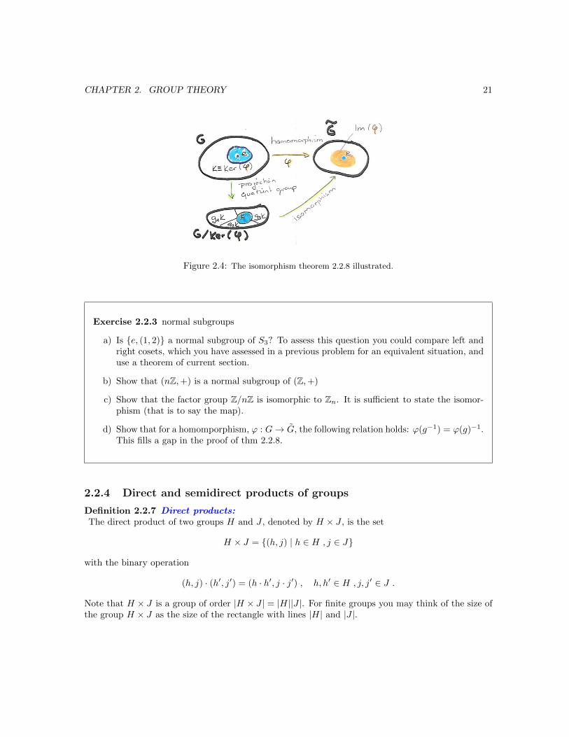
The isomorphism theorem is illustrated in Fig. 2.4. The essence of the first isomorphism theorem isthat to show that a group, say Ni is a normal subgroup, it is often simplest to find the homomor-phism where the kernel corresponds to Ni. The theorem will be applied to show that even and offpermutations are well defined (c.f. section 2.3.2).
11An interesting fact that emerged from the classification of finite groups is that all simple finite groups admit a setof generators which consists of at most two elements. From the simple groups all other finite groups can be built.
12There are two further isomorphism theorems frequently stated in textbook which we do not discuss in this course.13For a group homomorphism the Ker = g ∈ G|φ(g) = eG.14In the last step we, silently, used ϕ(k−1
2 ) = ϕ(k2)−1. You are going to fill in this step in exercise 2.2.3.
CHAPTER 2. GROUP THEORY 21
Figure 2.4: The isomorphism theorem 2.2.8 illustrated.
Exercise 2.2.3 normal subgroups
a) Is e, (1, 2) a normal subgroup of S3? To assess this question you could compare left andright cosets, which you have assessed in a previous problem for an equivalent situation, anduse a theorem of current section.
b) Show that (nZ,+) is a normal subgroup of (Z,+)
c) Show that the factor group Z/nZ is isomorphic to Zn. It is sufficient to state the isomor-phism (that is to say the map).
d) Show that for a homomporphism, ϕ : G→ G, the following relation holds: ϕ(g−1) = ϕ(g)−1.This fills a gap in the proof of thm 2.2.8.
2.2.4 Direct and semidirect products of groups
Definition 2.2.7 Direct products:The direct product of two groups H and J , denoted by H × J , is the set
H × J = (h, j) | h ∈ H , j ∈ J
with the binary operation
(h, j) · (h′, j′) = (h · h′, j · j′) , h, h′ ∈ H , j, j′ ∈ J .
Note that H × J is a group of order |H × J | = |H||J |. For finite groups you may think of the size ofthe group H × J as the size of the rectangle with lines |H| and |J |.

CHAPTER 2. GROUP THEORY 22
Definition 2.2.8 Semidirect products:Let φ be a group action of a group H on J then one can define a semi-direct product denoted byH n J . H n J is the set H × J with the following binary operation:
(h, j) · (h′, j′) = (h · h′, j · φ(h, j′)) ≡ (h · h′, j · (h.j′)) , h, h′ ∈ H , j, j′ ∈ J .
The order of H n J is |H| · |J | in close analogy to order of the direct product groups.
Examples 2.2.3 of semidirect products
- An example of the semidirect product is the group of euclidian isometries which consist of arotation R and a translation ~a which act on some vector space. Two consecutive applicationsgive rise to
((R′,~a′) · (R,~a)) ~x = (R′,~a′) ((R,~a) ~x) = (R′,~a′) (R~x+ ~a) = R′R~x+R′~a+ ~a′ (2.10)
and hence (R′,~a′) · (R,~a) = (R′R,R′~a + ~a′) 6= (R′R,~a + ~a′) is not equal to a direct productstructure. One writes ISO(n) = O(n) n Rn. In physics rotation and boosts plus space-timetranslations correspond to the so-called Poincare group whose invariants, the mass and the spin,characterise a particle. When the translations are omitted the group is referred to as the Lorentzgroup which is obviously a subgroup of the Poincare group. Hence the Poincare group is thesemidirect product of the Lorentz and the time-space translation group.
Figure 2.5: C2H6-molecule with D3-dihedral symme-try. Taken from [Ham62].
Figure 2.6: Triangle with D3-dihedral symmetry. Thedihedral symmetry Dn can be understood as the sym-metry of the regular n-polygon.
• Another important example comes from chemistry where many molecules (c.f. Fig. 2.5) arecharacterised by what is called the dihedral group, denoted by Dn, of order 2n which is a

CHAPTER 2. GROUP THEORY 23
semidirect product Zn o Z2.15 The group homomorphism of Z2 on Zn is given by inversion.16
In Fig. 2.5 the inversion is literally the inversion through the centre point of the molecule.Alternatively the dihedral group Dn is the symmetry group of a regular n-polygon as illustratedfor the triangle in Fig.2.6. The inversion (operation s in Fig. 2.6) corresponds to rotatingthe polygon by 180 around a straight line from a vertex through its centre. Examples for(ri, si) ∈ Zn o Z2 are
(e2πi3/n, 1) · (e2πi1/n, 1) = (e2πi4/n, 1)
(e2πi3/n,−1) · (e2πi1/n, 1) = (e2πi3/ne2πi(−1/n),−1) = (e2πi2/n,−1) , (2.11)
and hopefully clarify the text above. A presentation is given by,
Dn = < r, s | rn = s2 = s−1rsr = e > . (2.12)
The group element r corresponds to a rotation of 360/n around the axis of the molecule ands corresponds to the rotation around 180 of the centre of the molecule. For D3 the operationsare illustrated in Fig. 2.6. As already mentioned the dihedral group is the symmetry group ofmolecules. As another example we shall mention the symmetry of a snowflake which correspondsto D6 (hexagon).
Exercise 2.2.4 Products of groups.
a) Show that S3 is isomorphic to D3 by finding the elements of S3 (from the multiplicationtables) that satisfy the presentation 2.12. You could also attempt a geometric approachand identify the symmetries in either the C2H6-molecule Fig. 2.5 or Fig. 2.6.
b) As a matter of fact (up to isomorphisms) there are two groups of order six. One ofthem is D3. Can you find or give the other one?
c) The Vierergruppe Z2 × Z2 has got the following group presentation:
Z2 × Z2 = 〈a, b | a2 = b2 = (ab)2 = e〉 .
Write down explicit generators for a, b and ab in terms of the direct product notation:(e2πim/2, e2πin/2).
2.3 Permutation groups
2.3.1 The symmetric permutation group Sn
We have already mentioned the permutation group Sn in examples 2.1 and shown the multiplicationtable of S3 in table 2.2. In this chapter we shall discuss some more details.
15This is why some authors also denote the dihedral group of 2n elements by D2n.16Recall from exercises 2.1.4 that inversion, itself, is a group homomorphism for abelian groups which is clearly the
case for Zn.

CHAPTER 2. GROUP THEORY 24
Consider a set of n elements X = x1, ..., xn, then all possible permutations of this set, obviously,define a group which is denoted by Sn and called the symmetric permutation group.1718 ..Snleaves symmetric polynomials P (x1, x2, ..xn) The number of elements of this group corresponds to thenumber of possible permutations which is n!. The elements of the group can be denoted by brackets,as in table 2.2, (a1, a2, a3..) with 1 ≤ a−i ≤ n which correspond to cyclic permutations; best explainedby example:
(1, 4, 2) · (1, 2, 3)︸ ︷︷ ︸=(2,3,4)
xa, xb, xc, xd = (1, 4, 2) xc, xa, xb, xd = xa, xd, xb, xc . (2.13)
Once understood we can define multiplication directly within the group without reference to the setX, as indicated in Eq.(2.13). Other example which you may want to verify are:
(1, 2) · (2, 3) = (1, 2, 3) , (2, 3) · (1, 2) = (1, 3, 2) . (2.14)
A cycle (a1, .., ak) is referred to as a k-cycle and a 2-cycle is called a transposition . Without proof:All elements of Sn can be written as the product of disjoint cycles. By two disjoint cycles we meancycles (a1, .., an) and (b1, .., bm) for which ai 6= bj for 1 ≤ i ≤ n and 1 ≤ j ≤ m. any which do nothave any permutation element in common. Note that disjoint cycles commute with each other e.g.(1, 2)·(3, 4) = (3, 4)·(1, 2). Hence whenever two cycles are not disjoint one can commute them throughother elements and then multiply them into a single object as done above (2.14). You will providesome more evidence in exercise 2.4.1. Problems such as the question of how many m-cycles there arein Sn are very typical combinatorial problems that are best broken into parts. For example we mayfirst look at how many ways there are to get m distinct numbers out of n which is n!/(n−m)!/(m!).Second we take into account the ordering. We may freely choose one element to be in the first entryby convention but then the order of all the others matters and there are (m− 1)! possibilities. Hencethe answer is n!/(n−m)!/m. For example there 4!/(4− 3)!/3 = 8 3-cycles in S4:
(1, 2, 3), (1, 3, 2), (1, 2, 4), (1, 4, 2), (1, 3, 4), (1, 4, 3), (2, 3, 4), (2, 4, 3) . (2.15)
Theorem 2.3.1 The transpositions (2-cycles) generate Sn.
Proof: The elements of Sn consist of products of k-cycles with 1 ≤ k ≤ n. An arbitrary k-cycle canbe obtained from the following product of transpositions.
(a1, a2, ..., ak) = (a1, ak) · (a1, ak−1) · ... · (a1, a2) , q.e.d.
More specifically
Theorem 2.3.2 (a) The transpositions (1, 2), (1, 3), .., (1, n) generate Sn.(b) The transpositions (1, 2), (2, 3), .., (n− 1, n) generate Sn.(c) The transposition (1, 2) and the n-cycle (1, 2, .., n) generate Sn.
Proof: (a) Note that (a1, a2) = g · (1, a2) · g−1 , g = (1, a1) and then use theorem 2.3.1. (b)Note that (1, k) = g · (1, 2) · g−1 , g = (k − 1, k) · .. · (3, 4) · (2, 3) and then use (a). (c) Note that(k, k + 1) = g · (1, 2) · g−1 where g = (1, 2, .., n)k and then use (b) q.e.d.
The proof of (b) and (c) are in essence implementing a change of basis (relabelling the permutationelements).
17A more abstract definition for Sn are the maps that are bijections (one-to-one) on a set of n-elements.18Sn is the group which leaves so-called symmetric polynomials in n variables invariant.
CHAPTER 2. GROUP THEORY 25
2.3.2 The alternating group An
We have learned that any element of the symmetric group can be written as a product of k-transpositions.The number of transposition that occur are unambiguously even or odd and are called even- andodd-permutations respectively. This can be seen by using the first isomorporhism theorem 2.2.8.Consider the Vandermonde polynomial P (x1, .., xn) = (x1−x2)·..·(x1−xn)·(x2−xn)·..·(xn−1−xn)19
of all possible products of (xi − xj) with i 6= j. Then the map φ : acting on P/|P | by permutationis a group homomorphism from Sn to Z2 since the image of Sn acting on P is ±P and thereforeisomorphic to Z2. The kernel of this map are the even permutations i.e. An. The latter are therefore,according to theorem 2.2.8, a normal subgroup (i.e. An C Sn) of order |An| = |Sn|/|Z2| = n!/2.20
Stated as a theorem:
Theorem 2.3.3 alternating group An: The even-permutations generate a normal subgroup of Snof order n!/2
Proof: Given above.
Theorem 2.3.4 The 3-cycles generate An
Proof: According to theorem 2.3.2 Sn is generated (1, 2), (1, 3)... In the case of An each element,consists of an even number of transpositions. Since (1, a1) · (1, a2) = (1, a2, a1) the statement follows.q.e.d.
2.4 Platonic solids
A platonic solid is a regular, convex geometric body in three dimensions which consists of facesof a single polygon. There are five solids which meet this criteria, each named after the numberof polygons: tetrahedron, hexahedron (cube), octahedron dodecahedron, icosahedron, c.f. Fig. 2.7.Further information can be found in table 2.3. The symmetry of the platonic solids seems predestinedto be explained by group theory. The symmetry groups are given in table 2.3 on the right andcorrespond all to groups of the An- and Sn-type. An obvious start to characterise the symmetrygroup is to note that any symmetry permutes the vertices of the body. Hence the symmetry groupof a platonic solid with n vertices is a subgroup of Sn (in accordance with Cayley’s theorem 2.1.2).Intuitively the reason why it is not necessarily Sn is that the platonic solids have a certain rigidity sothat one can not arbitrarily permute the edges.
Moreover, platonic solids which are equivalent under interchange of vertices and surfaces are dualto each other; they have the same symmetry group. As can be seen from table 2.3 the tetrahedron isdual to itself and the hexahedron and octahedron (c.f. Fig. 2.8 in addition) as well as the dodecahedronand icosahedron are dual to each other respectively.
We would like to illustrate the symmetry group by looking at one specific example that is thetetrahedron. The symmetry operations are shown in Fig. 2.9. They consist of a rotation symmetryof 120 (denoted by r) around the axis of a vertex through the centre of the opposite face and a180 rotation through around an axis that goes through the middle of two opposite edges. From thefigure it is easily deduced that r and s correspond to (2, 3, 4)- and (1, 4)(2, 3)-permutation respectively.
19This is a so-called alternating polynomial. The name derives from the fact that the permutation of any two variablesalternates the sign and this is what gave the alternating group its name c.f. definition above.
20An C Sn also follows from theorem 2.2.7.

CHAPTER 2. GROUP THEORY 26
Figure 2.7: Platonic solids – photocopied from [Arm88].
solid faces vertices edges polygon symmetry grouptetrahedron 4 4 6 triangle A4
hexahedron 6 8 12 square S4
octahedron 8 6 12 triangle S4
dodecahedron 12 20 30 pentagon A5
icosahedron 20 12 30 triangle A5
Table 2.3: Platonic solids (c.f. Fig.2.7) with number of faces (F), vertices (V) and edges E), the polygonand their symmetry group. The former are related by the famous Euler formula: V − E + F = 2 which canbe proven in many ways. The hexahedron and octahedron as well as the dodecahedron and icosahedron aredual under interchange of the number of faces and vertices. This is the reason they admit the same symmetrygroup.
Those permutations are even and provide some evidence that the subgroup could be A4. You willcomplete a more thorough proof in the exercises below.
Exercise 2.4.1 Permutation groups.
a) In the notes it was stated that any element of Sn can be written as a product of disjointcycles for which we have not given a proof. This exercise aims to give some evidence byexample.Take (1, 2, 3) and (2, 4, 5) (common element 2) and write down the the 5-cycle correspondingto (1, 2, 3) · (2, 4, 5). Hint: In order to establish the multiplication rule let the cycles act ona set of five ordered elements.
b) Exercise a) will help you to answer the following question: What is the largest order of anelement in S10?

CHAPTER 2. GROUP THEORY 27
Figure 2.8: Octahedron and cube being dual under in-terchange of faces and vertices. Figure from [Arm88].
Figure 2.9: Tetrahedron (photocopied out [Arm88])
c) The symmetry group of the tetrahedron is isomorphic to A4. A presentation of A4 is givenby:
A4 = < a, b | a2 = b3 = (ab)3 = e > . (2.16)
Show that r = (2, 3, 4) and s = (1, 4)(2, 3), as defined above these exercises, satisfy thepresentation relation in (2.16).
d) The symmetry group of the cube is isomorphic to S4. For the cube it is appropriate toconsider the space diagonals as the group elements (They retain the rigidity of the cube.Think of the space diagonals as a scaffolding of the cube.) According to theorem 2.3.2 S4 isgenerated by (1, 2) and (1, 2, 3, 4). Identify those symmetry operations geometrically. Hint:Whereas the operation (1, 2, 3, 4) should be immediate, (1, 2) could be a bit more difficult.You could try to look for a symmetry operation which is of order two since (1, 2)2 = e.
e) List all 24 elements of S4 in the form (), (x, y), (x, y, z), (x, y, z, w) and (x, y) · (z, w) withx, y, z, w ∈ 1, 2, 3, 4.
f) Let S4 act on the sets 1) x1 = a, a, a, a 2) x2 = a, a, a, b, 3) x3 = a, a, b, c and 4)x4 = a, b, c, d by permutation. Give the stabiliser subgroup and the size of the orbit (writedown all elements of the orbits) for each set x1,2,3,4 and verify corollary 2.2.1.
2.5 Applications
Most applications of finite group theory involve representation theory which are going to treat insubsequent chapters. We shall content ourselves alluding at one (two) example(s) from chemistry

CHAPTER 2. GROUP THEORY 28
which can be found in [Atk08] chapter 11.
Figure 2.10: Water molecule H20 with Z2 symmetry. The water molecule has a permanent electric dipolemoment along the symmetry axis as further discussed in examples 2.5.1.
Examples 2.5.1 Polarity and chirality of molecules..
• A polar molecule is a molecule with a permanent electric dipole. The basic idea is that themolecule has to be asymmetric to a certain degree for it to admit an asymmetric charge distri-bution. The latter is the source of a permanent electric dipole. For instance any molecule thathas a Zn≥2-symmetry cannot have an electric dipole that is perpendicular to the symmetry axis.So it appears at first that C2H6 Fig. 2.5 and H2O (water) in Fig.2.10 could have an electricdipole along the rotation axis of Z3 and Z2 respectively. For C2H6 the s-symmetry operationFig.2.6 takes one end of the molecule to the other and this obstructs the formation of a electricdipole. Hence only H20, and not C2H6, has got a permanent electric dipole.
As a matter of fact only molecules with Zn-symmetry types (c.f. [Atk08] for more details)posses a permanent electric dipole along the rotation axis.
• Another example is the chirality of a molecule (mirror image not the same as the original); c.f.[Atk08]. A molecule may be chiral if does not admite an improper rotation axis. An improperrotation, is a rotation around an axis followed by an inversion.21 Since we did not discuss thosekind of symmetry groups we shall not go into any further details here.
21These groups are denoted, somewhat unfortunately, by Sn in the Schoenfliess notation used in chemistry literature.They are of order n and not to be confused with the permutation group of order n!.
Chapter 3
Representation theory
Representations are realisation of groups on linear vector spaces. Applications within mathematics,physics, computer science and so on are enormous. Especially from the viewpoints of sciences, otherthan pure mathematics, representation are natural since computations are performed in concretesettings such as linear spaces. From your course on quantum theory you are familiar with theconcept of discussing physics (equivalently) in different linear spaces. E.g. the harmonic oscillator canbe discussed in the coordinate space |x〉, momentum space |p〉 or the number of particle representation|n〉. Each one of them has its own merits. When in addition the system displays a symmetry, e.g.rotational symmetry of the potential, then the symmetry transformation acts as a representation onthe physical eigenstates of the Hilbert space. This will become clearer when we proceed to examples.
Discussion of finite representation theory, which consists to a large extent of character theory,is presented in chapter 4; followed by chapter 5 on Lie groups. In the current chapter we give thedefinition of a representation and discuss it in the, by now, familiar setting of S3. Basic definitionsare given in section section 3.2. Section 3.3 discusses Schur’s lemma and decomposability, which arerelevant both to finite representation theory of chapter 4 and the Lie groups of chapter 5. Applicationsare presented at the end of the chapters.
Definition 3.0.1 representation:
A representation ρ is a homomorphism (c.f. definition 2.1.3) from a group G into the set of linear(invertible) operators on a complex vector space V (the latter are denoted by GL(V ) and form agroup structure themselves under composition).
ρ : G −→ GL(V )
g −→ ρ(g) .
Since ρ is a homomorphism the map is compatible with the group structure, (c.f. Eq. (2.2)),1
ρ(g1 · g2) = ρ(g1)ρ(g2) . (3.1)
The relevant2 representations of finite groups are finite dimensional and therefore ρ(g)’s are nothingbut matrices acting on a finite dimensional vector space; i.e. V = Cn with n = dimV .
1Alternatively we may think of a representation as a group action on the linear space V .2i.e. irreducible, a terms to defined shortly hereafter
29

CHAPTER 3. REPRESENTATION THEORY 30
3.1 Representations the pedestrian way
Going back to the permutation group of three elements S3. According to theorem 2.3.2 a), S3 isgenerated by the elements (1, 2), (1, 3). Associating the permutation with permutation of unit vectorsof a three dimensional space we may represent those elements by:
ρ((1, 2)) =
0 1 01 0 00 0 1
, ρ((1, 3)) =
0 0 10 1 01 0 0
. (3.2)
All other elements may be generated from (3.2). Whereas this is certainly a representation, known asthe permutation representation , it does nor answer the following two questions: i) are there anyother representations? ii) can the representation be further reduced? We shall see that representationtheory of finite groups gives concrete and definite criteria for answering questions i) and ii). Beforepresenting the theory let us point out that one can see that the representation (3.2) can be furtherreduced. Both matrices, and therefore all group elements, have the eigenvector ~v = (1, 1, 1)T , witheigenvalue λ~v = 1, in common:
ρ((1, 2))~v = ~v , ρ((1, 3))~v = ~v . (3.3)
Hence one can construct a change of basis, ρ→ ρ′, such that the matrices are block diagonal
ρ′((1, 2)) =
1 0 00 a1 a2
0 a3 a4
, ρ′((1, 3)) =
1 0 00 b1 b20 b3 b4
. (3.4)
It is noted that the original three dimensional representation has split into a one and a two dimensionalrepresentation. Representations which can be split as the one in Eq. (3.2) are called reducible. Arepresentation which cannot be split any further is called an irreducible representation. An aim ofrepresentation theory is to find, and if possible construct, all irreducible representation of the group.It is now time to proceed to the more formal representation theory.
Exercise 3.1.1 Representations the pedestrian way
a) Verify through explicit matrix multiplication that the product ρ((1, 2))ρ((1, 3)) in (3.2)generates an element which can be interpreted as ρ((1, 3, 2)) in terms of permutation of theunit vectors.
3.2 Basic definitions of representation theory
Representations have been defined in definition 3.0.1 and we have seen a first example in section 3.1.Below ρ(g) denotes a representation of g ∈ G on the vector space V .
Definition 3.2.1 of representation theory

CHAPTER 3. REPRESENTATION THEORY 31
• A representation is faithful if the homomorphism ρ is injective (inverse map from image isdefined). If the latter is not the case the representation is called unfaithful accordingly. Ifρ(g) = ρ(e) for ∀g ∈ G then the representation is called the trivial representation .
• A unitary representation is a representation for which ρ(g) is a unitary operator on thevector space.
• Two representations ρ and ρ′ are called equivalent if they can be mapped into each other bya similarity transformation . I.e. if there exists S ∈ GL(V ) s.t. ∀g ∈ G, ρ(g) = Sρ′(g)S−1.3
• An invariant subspace is a subspace W ⊂ V which is left invariant by the representationacting on it i.e.
ρ(g)~w ⊂W , ∀~w ∈W ,∀g ∈ G . (3.5)
• A representation is irreducible if there are no invariant subspaces.
Fact: If there are invariant subspaces one can find a basis where ρ(g) can be written as
ρ(g) =
(ρ1(g) 0
0 ρ2(g)
), ∀g ∈ G , (3.6)
in a block diagonal form.4 If a representation can be written in the form (3.6) the representationis said to be reducible .
In essence a representation is either irreducible or reducible. For finite groups (c.f. theorem3.3.3) and continuous groups which are compact the reducible representations are a direct sumof the irreducible representations.5
• A real representation is a representation which can be brought (similarity transformation)into a form where the matrix entries are all real numbers. If this is not the case we speak of acomplex representation .6 The complex conjugate representation of ρ is denoted by ρ = ρ∗
and is given by complex conjugation (of the matrix entries).
Unitary representations are of importance for quantum physics. Unitary transformations are thenatural language to describe symmetries on the physical Hilbert space since they preserve the innerproduct. Irreducible representation are not only the atomic objects of mathematical representation the-ory but they are also the ”atoms” in physics. According to Wigner an elementary particle correspondsto an irreducible representation of the Poincare group (i.e. space-time symmetry group includingtranslations.) In physics, or particle physics, complex representation are associated with charges; realrepresentations carry no charge.
Exemplifying some of these terms for the representation discussed in (3.2). The representation(3.2) is reducible since it can be written in block diagonal form (3.4). The two representations (3.2)and (3.4) are equivalent. The representation ρ′ (and therefore also ρ since it is equivalent ) containthe trivial representation which is in particular unfaithful. The representation ρ is real since thecorresponding matrices have real entries. The representation ρ′ is real since it is equivalent to therepresentation ρ which is real.
3As the wording suggest the equivalence of representations is an equivalence relation.4We omit the proof of this statement.5We shall give an example of a non-reducible representation for the translation group (which is non-compact) in
chapter 5.6For SU(2) we will encounter a refinement of this notion to so-called pseudo-real representations.
CHAPTER 3. REPRESENTATION THEORY 32
3.3 Basics of representation theory Maschke’s thm, Schur’sLemma and decomposability
In this section we state a few facts about representation theory of finite groups which are also relevantfor representation theory of the Lie groups (compact Lie groups U(1), SO(2), SO(3) and SU(2))which are going to discuss in the chapter 5. The theorems are stated for finite groups.
Theorem 3.3.1 Maschke’s thm:Any representation of a finite group is equivalent to a unitary representation.
Proof: Suppose (x, y) is the inner product of the vector space. One can define a new inner product
(x, y)G ≡1
|G|∑g∈G
(ρ(g)x, ρ(g)y) (3.7)
by averaging over the group (Weyl’s trick). It is easily verified (exercises) that ρ(g) is unitary i.e.(ρ(g)x, ρ(g)y)G = (x, y)G with respect to the new inner product. q.e.d.
Theorem 3.3.2 Schur’s LemmaLet ρ and ρ′ be two irreducible representations of vector spaces V and V ′ and T : V → V ′ be a linear
map satisfying ρ′T = Tρ then
a) T is either an isomorphism, or T = 0 is trivial.
b) If V = V ′ then T = λ · 1 (for λ ∈ C and 1 the identity map on V ).
Schur’s lemma states in essence that there is no room for any non-trivial homomorphisms betweenirreducible representations of a group. Schur’s Lemma is the fundament of representation theory. Itis the essential ingredient to many powerful theorems. Often you will find Schur’s lemma stated asfollows: let ρ be a matrix irreducible representation and T a matrix in the same space with [T, ρ(g)] = 0for ∀g ∈ G then T = λ1. This is clearly equivalent to theorem 3.3.2b).
Proof: a) The first statement follows from the fact that Ker(T ) and Im(T ) are invariant subspaces (tobe discussed below) and therefore Ker(T ) = 0, V and Im(T ) = 0, V ′ since irreducible representationdo not admit non-trivial invariant spaces. If Ker(T ) = 0 then Im(T ) = V ′ and T is an isomorphismby virtue of the first isomorphism theorem 2.2.8. If Ker(T ) = V then Im(T ) = 0 and T = 0 (maps allelements into zero vector of V ′.)
Remains to be shown that Ker(T) = v0 ∈ V | Tv0 = 0 is an invariant subspace i.e. Tρ(g)v0 = 0.This follows from Tρ(g)v0 = ρ′(g)Tv0 = 0 by using the premise Tρ(g) = ρ′(g)T .
b) If T = 0 then λ = 0. If T 6= 0, T must have at least one eigenvalue λ. Hence for U ≡ T − λ1,dim[ker(U)] ≥ 1 and U is not an isomorphism; by virtue of a) U = 0; i.e. T = λ1 q.e.d.
Theorem 3.3.3 Decomposability thm
a) Any reducible representation of a finite group decomposes into irreducible representations,
ρ(g) = m1ρ1(g)⊕ ..⊕mkρk(g) , (3.8)
with multiplicities mi ∈ Z+.7
7A representation is simply reducible if mi = 0, 1.
CHAPTER 3. REPRESENTATION THEORY 33
b) The decomposition into k factors is unique whereas the decomposition into a direct sum of mi
copies is not.
Proof: a) We content ourselves with the remark that the proof uses the same inner product as intheorem 3.3.1. b) Consider another representation of ρ′ = m′1ρ
′1 ⊕ .. ⊕ m′Kρ′K of G in V and T a
map between those representations. Then it follows from Schur’s lemma that T must map ρi to ρ′iwhich are isomorphic to each other. (One cannot map a representations of different dimensions toeach other as otherwise T would not correspond to an isomorphism.) q.e.d.
Exercise 3.3.1 a) Argue that a representation ρ(g) is unitary with respect to the inner prod-uct (3.7). I.e. (ρ(g)x, ρ(g)y)G = (x, y)G.

Chapter 4
Representation theory of finitegroups
4.1 Character theory for finite groups
The character theory is the heart of the representation theory of finite groups.
Definition 4.1.1 The trace of a representation ρ is called the character χ
χ(g) ≡ Tr[ρ(g)] . (4.1)
Hence to each group element a character is associated. The following properties are immediate:
Corollary 4.1.1 (of definition 4.1.1):
a) The characters of two equivalent representation (c.f. 3.2.1) are equal:
χ(Sρ(g)S−1) = Tr[Sρ(g)S−1] = Tr[ρ(g)] = χ(g) . (4.2)
b) The characters of conjugate elements are identical for the same reason as in a) (replace S → ρ(g′)above). It is therefore sufficient to consider conjugacy classes only. The character is said to bea class function (its value is constant on any conjugation class of a representation).
c)
χ(ρa ⊕ ρb) = χ(ρa) + χ(ρb) , (4.3)
χ(ρa ⊗ ρb) = χ(ρa) · χ(ρb) , (4.4)
χ(ρ(g−1)) = χ(ρ(g))∗ . (4.5)
Above the index a and b are labels referring to a type of representation (e.g. trivial, permutationrepresentation in the case of Sn). The first two properties follow from (1.18) and (1.20) andthe definition of the trace respectively. The last property (4.5) is a consequence of Maschke’stheorem 3.3.1:
χ(ρ(g−1)exercise(2.2.3)
= χ(ρ(g)−1) = χ(ρ(g)†)Tr[AT ]=Tr[A]
= χ(ρ(g)∗) = χ(ρ(g))∗ . (4.6)
34
CHAPTER 4. REPRESENTATION THEORY OF FINITE GROUPS 35
Maschke’s thm was used in the second equality.
• d) For one dimensional representations the character is equal to the representation matrix sincethe latter is a 1 × 1-matrix. Note that a one dimensional representation is not necessarily thetrivial representation.
The characters characterise groups to a large extent. In fact the mathematician Gerhard Brauerasked the question whether the characters together with the order of the elements would completelydetermine a finite group. It took decades to find a counterexample and this shows how importantcharacter tables are.
Definition 4.1.2 One can define an inner product on the space of characters as follows:
〈χ(ρa)|χ(ρb)〉 ≡ 1
|G|∑g∈G
χ(ρa(g))∗χ(ρb(g))
=1
|G|
Nc∑k=1
ckχ∗akχbk . (4.7)
Above χak = χ(ρa(gk)) with gk belonging to the kth-class with ck elements. The number Nc denotesthe total number of classes of the group. The second line exploits the fact that the character is aclass function. The character χ(g) can be thought of as a vector in CNc where each class represent alinearly independent direction:
χ(ρ) = (χ(ρ(e)), ..., χ(ρ(gNc)) ∈ CNc , (4.8)
where gNc , as above, is a representative of the Ncth-class. Note, the first class is usually assigned to
the identity element.
Theorem 4.1.1 Orthogonality theoremIn terms of the inner product (4.7) the irreducible representations of G are orthonormal, i.e.
〈χ(ρa)|χ(ρb)〉 = δab . (4.9)
The proof is given for the interested reader only as it is too abstract for a first course on represen-tation theory. Let us just mention that the main ingredient is Schur’s lemma.
CHAPTER 4. REPRESENTATION THEORY OF FINITE GROUPS 36
for the interested reader (not part of the course)
Proof: Let us assume that Va and Vb are irreducible representations of G. Then the spaceof all homomorphism from Va → Vb is equal to Hom(Va, Vb) = V ∗a ⊗ Vb where V ∗a is the dualvector space of Va (going from ket to bra in Dirac notation). Let V0 denote the vector spaceof trivial representations i.e. ρ(g)|V0
= 1V0, , ∀g ∈ G.
The rest of the proof builds on three observations: i) Schur’s lemma states that the onlynon-trivial homomorphism, compatible with the group structure (i.e. invariant), there canbe is an isomorphism. Hence dim(Hom(Va, Vb)0) = δab where the subscript zero denotes thetrivial representation subspace as before. ii) The character of the V ∗a ⊗ Vb representation isgiven by
χ(ρV ∗a ⊗Vb)(4.4)= χ(ρV ∗a ) · χ(ρVb) = χ(ρVa)∗ · χ(ρVb) , (4.10)
where ρVa ≡ ρa in the statement of the theorem. iii) The operator φ = 1|G|∑g∈G ρV (g) is a
projector (φ2 = φ) on V0. I.e. φv0 = v0 ,∀v0 ∈ V0 and φV ⊥0 = 0 where V ⊥0 ⊕ V0 = V . Tosee this note that applying φ to a vector results in an invariant vector and the only invariantvectors corresponds to the subspace of trivial representation. Moreover, a second applicationof φ just results in a rearrangement which has though no effect since it is averaged over thegroup and therefore φ2 = φ. Hence the number of trivial representation is given by
dim(V0) = Tr[φ] =1
|G|∑g∈G
χ(ρV (g)) . (4.11)
Assembling
δabi)= dim(Hom(Va, Vb)0) = dim((V ∗a ⊗ Vb)0)
iii)=
1
|G|∑g∈G
χ(ρV ∗a ⊗Vb(g))
ii)=
1
|G|∑g∈G
χ(ρVa(g))∗ · χ(ρVb(g))def= 〈χ(ρVa)|χ(ρVb)〉 , q.e.d. (4.12)
Corollary 4.1.2 (of the orthogonality theorem 4.1.1)Let ρ = m1ρ1 ⊕ ..mkρk stand for a generic representation.
a) A representation is fully characterised by its character since the distinct ρi’s correspond to
linearly independent vectors in χ(ρ(g))(4.3)= m1χ(ρ1(g)) + ..+mkχ(ρk(g)). You should think of
χ(ρ(g)) as a vector in CNc .
b) The multiplicity ma of ρa in ρ is given by
ma = 〈χ(ρa)|χ(ρ)〉 . (4.13)
c) The norm of a representation is
||χ(ρ)||2 = 〈χ(ρ)|χ(ρ)〉 =∑i
m2i . (4.14)

CHAPTER 4. REPRESENTATION THEORY OF FINITE GROUPS 37
Hence ρ is irreducible ⇔ ||χ(ρ)||2 = 1.
d) The character of the identity element corresponds to the dimension of the representation:
χ(ρi(e)) = dimVi (4.15)
e) The characters of the trivial representation are all one. I.e.
χ(ρ1) = (1, .., 1) ∈ CNc . (4.16)
Exercise 4.1.1 Characters:
a) Verify statements b),c), d) and e) in corollary 4.1.2
b) Obtain all six matrices of the representation (3.2). Two are given, one is trivial and oneof them you have already computed in exercise 3.1.1. Compute the remaining two andcompute the norm of the character using the inner product (4.7).
c) According to the decomposability theorem 3.3.3 the permutation representation is either adirect sum of i) three one dimensional or ii) one one dimensional and a two dimensionalirreducible representation. I.e. ρperm = ρ1+ρ1′+ρ1′′ or ρperm = ρ1+ρ2 where the subscriptdenotes the dimension of the representation. Using the result in b) and a statement incorollary 4.1.2, show that ii) is the case.
d) Identify the equivalence classes of S3. You may for instance guess them and verify themeither through 1) explicit computation of the matrices 2) the multiplication laws from themultiplication table 2.2 or 3) you may proceed along the lines of proof of theorem 2.3.2 andfind the equivalence transformations. You might even want to try more than one methodto gain some confidence in the formalism. Note for S3 members of an equivalence classcorresponds to a renumbering of the elements so that guessing the equivalence classes ispossible.
In order to proof the powerful dimensionality theorem we are going to introduce the regularrepresentation
Definition 4.1.3 The regular representation corresponds to the left-action of the group on itself.More precisely to each element g ∈ G we associate a vector ~eg (declaring ~eg to be linearly independentof ~eg′ for g 6= g′) and the representation acts as follows:
ρR(g)~eg′ = ~eg·g′ . (4.17)
The regular representation has got the following property
χ(ρR(g)) =
0 g 6= e|G| g = e
, (4.18)
which follows from the fact the ρR(e) = 1|G| and that no other element than ρR(e) has any entry onthe diagonal (to be verified in the exercises).
CHAPTER 4. REPRESENTATION THEORY OF FINITE GROUPS 38
This definition together with the observation (4.18) is sufficient to proof the dimensionality theo-rem:
Theorem 4.1.2 Dimensionality theoremThe sum of the dimension squared of all irreducible representations of a finite group is equal to the
order of the group
|G| =Nc∑i=1
dim(Vi)2 . (4.19)
Proof: First we observe that
mi(4.13)
= 〈χ(ρi)|χ(ρR)〉 def=
1
|G|∑g∈G
χ(ρi(g))∗χ(ρR(g))(4.18)
= χ(ρi(e))(4.15)
= dim(Vi) . (4.20)
Second by virtue of the decomposability theorem 3.3.3 we may write
χ(ρR(g)) =∑i
miχ(ρi(g))(4.20)
=∑i
dim(Vi)χ(ρi(g)) (4.21)
and choosing g = e with Eqs. (4.18) and (4.15) we get
|G| =∑i
dimV 2i
which completes the proof q.e.d..
Note, had we known the dimensionality theorem earlier, the reducibility of the representation(3.2) would have been clear. Moreover exercise 4.1.1 could have been solved more efficiently. You cancomplete the argument in exercise 4.1.2 a).
Exercise 4.1.2 dimensionality thm
a) Use the dimensionality theorem to argue that the largest irreducible representation of S3 isof dimension two.
b) What is the dimension of the permutation and the regular representation of Sn?
c) Is the regular representation always reducible?
4.2 Character tables
The information on characters is commonly presented in terms of so called character tables; e.g.table 4.1 (a few pages ahead). First all group elements are divided into equivalence classes under con-jugation. Note the identity is always a conjugation class on its own. At the top row a representative
CHAPTER 4. REPRESENTATION THEORY OF FINITE GROUPS 39
of each equivalence class is listed. Sometimes a second row is present stating the order of the repre-sentative. To each successive row an irreducible representation is associated where the correspondingcharacters are listed. The fact that the table, without counting the top rows, can be interpreted as aunitary square matrix (to be made precise) is going to be one of the main results of this chapter.
The rows in the character tables can be thought of as linearly independent vectors by virtue ofthe orthogonality theorem 4.1.1. Each conjugation class defines a linearly independent direction.Hence it is clear that the number of irreducible representations of G is less or equal to the number ofequivalence classes as otherwise the rows would not be linearly independent. In fact they are equal:
Theorem 4.2.1 Character table is a square: The number of irreducible representations of G isequal to the number of conjugacy classes of G.
An equivalent statement is that the characters form an orthonormal basis for the class function space.Much alike exp(2πix/Ln), for n ∈ Z, form a basis for periodic function f(x + L) = f(x) in Fouriertheory. The proof of this theorem will be presented below but is not really part of the course and isgiven for the interested reader only. It is powerful but a bit abstract for an introductory course onthe subject.
for the interested reader (not part of the course)
Proof: Assume that there was a class function f : G→ C (c.f. definition 4.1.1) s.t.
〈f |χ(ρi)〉 = 0 (4.22)
on all irreducible representations. If we can show that f = (0, ..., 0) ∈ CNc , then the theoremis proven as this implies that the characters form a complete set of vectors on the class functionspace. Consider the following map,
φ =∑g∈G
f(g)∗ · ρi(g) : Vi → Vi , (4.23)
on the vector space Vi of the irreducible representation ρi. From ρi(g′)φ = φρi(g
′) and Schur’slemma (theorem 3.3.2) it follows that φ = λ1 and we may write:
λ dim(Vi) = Tr[φ] =∑g∈G
f(g)∗χ(ρi(g)) = |G|〈f |χ(ρi)〉(4.22)
= 0 . (4.24)
Hence either λ = 0 (i.e. f(g) = 0 for ∀g ∈ G) or∑g∈G f
∗(g)ρi(g) = 0 has to hold on anyirreducible representation and by virtue of decomposability on any representation; in particu-lar the regular representation ρR(g) (which is a direct sum of the irreducible representations).Since all ρR(g) are linearly independent by definition this enforces f(g) = 0 for all g ∈ G andthis completes the proof q.e.d.Note, we have therefore shown that no f other than f = (0, .., 0)obeys (4.22).
Another powerful theorem, somewhat reminiscent, of Lagrange’s theorem is:
CHAPTER 4. REPRESENTATION THEORY OF FINITE GROUPS 40
Theorem 4.2.2 The dimension of any irreducible representation divides the order of the group:
|G|dimVi
∈ Z+ , ρi is an irreducible representation on Vi (4.25)
We shall omit the proof1 and state simple corollary:
Corollary 4.2.1 All irreducible representations of an abelian group are one dimensional.
Proof: First we notice that for an abelian group each element forms a conjugacy class on its own sincea = g ·a · g−1 ⇔ a · g = g ·a. Hence for an abelian group there are as many irreducible representationsas there are elements by virtue of theorem 4.2.2. In order to obey the constraint (4.19) all those
irreducible representations are necessarily one dimensional∑|G|i=1 dim(Vi)
2 =∑|G|i=1 12 = |G| q.e.d.
Exercise 4.2.1 Representations of abelian groups By virtue of corollary 4.2.1 representa-tions of abelian groups are rather straightforward. You might find the following exercises usefulas they clarify previous matters.
a) Write down all irreducible representations of Z7. By virtue of corollary 4.2.1 they are onedimensional and in fact you have been using them in a previous exercise.
b) How many of the irreducible representations of the previous exercise are faithful?
c) How many irreducible representations of Z4 are faithful?
The amount of a priori information on the dimension of the irreducible representations is ratherimpressive and is largely grounded in the Schur’s important Lemma (theorem 3.3.2). In summary,given a finite group its irreducible representation ρi on Vi are constrained as follows:
Diophantine equations for dimVi of G
(1) |G| = 1 + dimV22 + ..+ dimVk
2 , (theorem 4.1.2)
(2) k = Nc ≡ number of conjugacy classes (theorem 4.2.1)
(3) |G|/ dim(Vi) ∈ Z+ , (theorem 4.2.2)
(4.26)
Note the one in |G| = 1 + .. stands for the trivial representation which is always present. Theequations above, diophantine nature, are in many cases sufficient to obtain the dimensions of theirreducible representations (without working them out explicitly). From the orthogonality 4.1.1 andthe fact that the character table is essentially a unitary matrix follows a second orthogonality theorem:
1In fact an even stronger statement applies: |G/Z(G)|/ dimVi is an integer where Z(G) is the centre of the groupwhich is always normal in the group itself.

CHAPTER 4. REPRESENTATION THEORY OF FINITE GROUPS 41
Theorem 4.2.3 Second orthogonality thm: We can define an inner product on the class space,with symbols as in (4.7), as follows:
〈χ(ρ([g])|χ(ρ([g′])〉C =c[g]
|G|
Nc∑i=1
χ(ρi([g])∗χ(ρi([g′]) . (4.27)
which is orthonormal,〈χ(ρ([g])|χ(ρ([g′])〉C = δ[g][g′] , (4.28)
in the class directions. The subscript C stands for class and helps to avoid confusion with the previousinner product (4.7). Note, the slightly asymmetric definition in (4.27) anticipates the result (4.28).
Proof: The proof is constructive and uses the fact that for a unitary n× n matrix U :
UU† = U†U = 1n . (4.29)
The second equation follows from the first by hermitian conjugation. The matrix U in our case is
Ua[g] =
(ck|G|
)1/2
χ(ρa([g]) , (4.30)
where we remind the reader that a and [g] are indices referring to an irreducible representation anda class representative respectively. The first and second orthogonality relations (4.9) and (4.28) canbe written as
〈χ(ρa)|χ(ρb)〉 = (UU†)ab =∑[g]
Ua[g]U∗b[g] = δab ,
〈χ(ρ([g]))|χ(ρ([g′]))〉 = (U†U)[g][g′] =
Nc∑a=1
U∗a[g]Ua[g′] = δ[g][g′] , (4.31)
where we implied the notation (U†)ab = U∗ba. Hence (4.30) guaranties that the two orthogonalityrelations imply each other. Stated differently: (4.9) ⇔ (4.28) q.e.d.
4.2.1 Character table of S3 as an illustration
We shall exemplify the character table of S3. The conjugacy classes correspond, for any permutationgroup Sn, to the number of ways in which n can be written in terms of integers. The latter is knownas a partition of an integer number n = λ1 + ....λk, λ1 ≥ .. ≥ λk ≥ 1. For S3 we have got:
3 = 1 + 1 + 1 ↔ [()] , 1 element , (4.32)
3 = 2 + 1 ↔ [(1, 2)] , 3 elements (4.33)
3 = 3 ↔ [(1, 2, 3)] , 2 elements . (4.34)
Hence there are three irreducible representations. We can start building the character table:
S3 class () (1, 2) (1, 2, 3)dim class 1 3 2
trivial 1 1 1alternating 1 −1 1
.. .. .. ..
(4.35)

CHAPTER 4. REPRESENTATION THEORY OF FINITE GROUPS 42
S3 class () (1, 2) (1, 2, 3)dim class 1 3 2trivial 1 1 1alternating 1 −1 1standard 2 0 −1
Table 4.1: Character table of S3 (which is isomorphic to D3).
With the class in the first row and the dimension of the class in the second row. The latter is oftenomitted. The trivial representation is always present and all its entries are equal to 1. For thepermutation groups Sn there is always a second one dimensional representation which acts as follows:
ρalt(g)~v = sgn(g)~v , (4.36)
where sgn(g) = ±1 depending on whether g is an even or odd permutation. There are many waysto know that the remaining irreducible representation is two dimensional c.f. exercise 4.2.2. In factthe permutation representation (3.2) decomposes into the trivial and the two dimensional irreduciblerepresentation : ρperm = ρtriv⊕ρstand (permutation, trivial and standard have been abbreviated.) Thestandard representation for the permutation groups is the non-trivial irreducible representationcontained in the permutation representation.
In the case of S3 the standard representation is two dimensional (c.f. exercise 4.1.2a) ). By virtueof exercise 4.2.2 the character of the permutation representation is equal to the number of elementsthat the operation leaves in invariant it follows that χ(ρperm.) = (3, 1, 0) in the order of the classes asin the character table. Therefore
S3 : (3, 1, 0) = χ(ρperm.)(4.3)= χ(ρtriv.) + χ(ρstand) = (1, 1, 1) + χ(ρstand) , (4.37)
which yields χ(ρstand) = (2, 0,−1) and completes the S3 character table 4.1.
Exercise 4.2.2 characters and orthogonality
a) Let ρperm be the permutation representation, as given for S3 in (3.2). Argue that χ(ρperm(g))corresponds to the number of elements that are left invariant by ρperm(g) acting on its vectorspace. The answer can be as short as one sentence.
b) Verify the second orthogonality theorem 4.2.3 on the example of the character table of S3
given in table 4.1.
Exercise 4.2.3 Step by step construction of the S4 character table.
a) Find all the character classes of S4 following the same recipe as for S3. Hint: You shouldfind that there are five of them.

CHAPTER 4. REPRESENTATION THEORY OF FINITE GROUPS 43
b) Argue that the irreducible representations satisfy the following equation:
24 = 12 + 12 + d23 + d2
4 + d25 (4.38)
Hint: the two 12 correspond to two one dimensional irreducible representations. Whichones?
c) Find the dimension d3,4,5 of the remaining three irreducible representations. The equationare “diophantine enough” to be solved.
d) Begin to build up the character table by writing down the first two irreducible representa-tions.
e) Find the character of the standard representation using the same method as for S3 (recall:ρperm = ρtriv ⊕ ρstand).
f) You can find another representation by multiplying the standard representation by thenon-trivial one dimensional representation.
g) You can find the character entries of the last irreducible representation by making sure thatit is orthogonal to the other entries. Hint: the class-characters assume the following values:0, 0,−1, 2, 2.
4.3 Restriction to a subgroup – branching rules
Before addressing the problem of restriction to a subgroup it will prove useful (in this context as wellas for the rest of the course) to expand on the definitions of real and complex representations givenin definition 3.2.1.
4.3.1 Complex and real representations
For a complex representation the complex conjugate representation ρa = ρ∗a is inequivalent. For a realrepresentation one can find a basis where ρa is real and therefore two complex conjugate representationare equivalent to each other. This knowledge gives a simple criterion, which we call the complex-real
CHAPTER 4. REPRESENTATION THEORY OF FINITE GROUPS 44
criterion , for determining the type of representation2
〈χ(ρa)|χ(ρa)〉 =1
|G|∑g∈G
χ(ρa(g)2)∗ =
0 ρa complex1 ρa real
. (4.39)
The first equality is by no means trivial but follows from the decomposition of V ⊗V into a symmetricand antisymmetric part as discussed in the footnote. In practice representations are often denoted bytheir dimension and if there is ambiguity then one uses prime or other symbols to distinguish them.In this spirit we write the complex conjugate representation as
complex conjugate representation of [3] ≡ 3 , (4.40)
where we have taken a three dimensional representation as an example for the sake of explicitness.
4.3.2 Branching rules
When a representation ρ(g) for g ∈ G is restricted to a subgroup H ⊂ G, ρ(h) certainly forms arepresentation since ρ is still a group homomorphism on a linear space. The crucial point is thoughthat it is not necessarily an irreducible representation. By virtue of the decomposability theorem therepresentation of G decomposes into irreducible representations of H
ρ(g)|H = m1ρ1(h)⊕ ...⊕mkρk(h) . (4.41)
where k is the number of equivalence classes of H.3
Branching rules can be constructed systematically from the character tables of the group G andH. In some cases, rather often, one is able to guess the branching rules with less information. Weillustrate this after pursuing the systematic construction.
We consider the example of Z3 ⊂ S3 and identify the branching rules. In doing so many conceptsof the previous sections get illustrated. First of all we note that since Z3 is abelian, c.f. corollary4.2.1, the irreducible representations of Z3 are all one dimensional. The group Z3 is generated byeither (1, 2, 3) or (1, 3, 2) and has therefore no transpositions (2-cycles). We denote the irreducible
2For completeness (non-examinable) let us mention that there is in addition there is a pseudo-real (or quaternionic)type representation where ρa = S−1ρaS exists but it is not a real representation. Fortunately there is a criterion forpseudo-reality: ρ(g) is pseudo-real if and only if 1
|G|∑g∈G χ(ρ(g)2) = −1. Note 〈χ(ρ)|χ(ρ)〉 = 1 for a pseudo-real
representation. Pseudo-real representations will be discussed in the context of the Lie group SU(2) in the followingchapter. In case you want to understand of why a pseudo-real representations are a logical possibility you may want toconsider exercise 3.38 in [Ful91]. The essential idea is that if the V is the vector space of a non-complex representationthen V ⊗V contains a trivial representation. The tensor product V ⊗V = Sym(V ⊗V )⊕Asym(V ⊗V ) decomposes into asymmetric and antisymmetric subspace similar to the case of a matrix that can be decomposed uniquely into a symmetricplus a antisymmetric matrix. In the case where the trivial representation falls into the Sym(V ⊗ V ) the representationis real and if it falls into Asym(V ⊗ V ) it is pseudo-real. The criterion for pseudo-reality is 1
|G|∑g∈G(ρ(g2)) = −1.
An example is given by the two dimensional representation of the Quaternions. The Quaternions are defined throughthe presentation Q8 =< I, J,K,−e | I2 = J2 = K2 = IJK = −e, (−e)2 = e >. The two dimensional representation isgiven by ρ2(I) = iσ3, ρ2(J) = iσ2 and ρ2(K) = iσ1 where σi are the well-known Pauli-matrices to be defined later on.One readily obtains that 1
|G|∑g∈G χ(ρ2(g)2) = 1
8(2 · 2 + 6 · (−2)) = −1.
3In the physics literature such decompositions are frequently called branching rules. Branching rules are importantin the case where a large symmetry breaks into a smaller one such as in grand unification e.g. SU(5) → SU(3) ⊗SU(2)⊗ U(1) with the latter being the gauge group of the so-called Standard Model.

CHAPTER 4. REPRESENTATION THEORY OF FINITE GROUPS 45
representations by 1Z3 , 1′Z3, 1′′Z3
. The irreducible representations of 1′Z3, 1′′Z3
are easily guessed to be
ρ(1, 2, 3)|1′Z3 = e2πi/3 ⇒ ρ(1, 3, 2)|1′Z3 = e−2πi/3 ,
ρ(1, 2, 3)|1′′Z3 = e−2πi/3 ⇒ ρ(1, 3, 2)|1′′Z3 = e2πi/3 . (4.42)
Notice that the 1′Z3, 1′′Z3
are complex representations (c.f. definition 3.2.1). In the case under discussionthey are necessarily complex conjugate representations of each other since they originate from S3 whoserepresentations are real. In terms of equations, using the notation introduced in Eq. (4.40),
1′Z3
= 1′′Z3, 1
′′Z3
= 1′Z3, (4.43)
where the second equation is just the complex conjugate of the first one. This knowledge can help inguessing the branching rules as we shall see below.
The characters are equal to the expressions in (4.42) since the representation is one dimensional.Below we give the character table for Z3 and reprint the character table of S3 in tables 4.2 and2.2 respectively. Note the elements (1, 2, 3) and (1, 3, 2) which are in the same equivalence class inS3 constitute different equivalence classes in Z3. This happens frequently and is due, in this case,to the fact that the transpositions (x, y), which guarantee the equivalence under S3 are not in Z3!Given both character tables one can compute the branching rules by taking scalar products of the
Z3 class () (1, 2, 3) (1, 3, 2)dim class 1 1 11 1 1 11′ 1 e2πi/3 e−2πi/3
1′′ 1 e−2πi/3 e2πi/3
Table 4.2: Character table of Z3.
S3 class () (1, 2) (1, 2, 3)dim class 1 3 2trivial (1) 1 1 1alternating (1′) 1 −1 1standard (2) 2 0 −1
Table 4.3: Character table of S3 reprinted from table2.2 for the readers convenience
corresponding characters. The question of how many times a representation j of Z3 is contained inthe representation i of S3,
ρ(S3)i |Z3=⊕j
mijρ(Z3)j (4.44)
can be obtained by the scalar product of the characters restricted to the subgroup Z3:
mij = 〈χ(ρ(S3)i |χ(ρ(Z3)j 〉Z3 =1
|Z3|∑h∈Z3
χ(ρ(S3)i(h))∗χ(ρ(Z3)j (h)) , (4.45)
where the right hand side resolves the potential ambiguity in notation between ρ(S3) and ρ(Z3) in thesame scalar product. This leads to the following branching rules:
branching rules: ρ1S3 |Z3 = 1 · ρ1Z3, 1S3 → 1Z3
ρ1′S3|Z3 = 1 · ρ1Z3
, 1′S3→ 1Z3
ρ2S3 |Z3= 1 · ρ1′Z3 ⊕ 1 · ρ1′′Z3 , 2S3
→ 1′Z3⊕ 1′′Z3
, (4.46)

CHAPTER 4. REPRESENTATION THEORY OF FINITE GROUPS 46
since the only non-vanishing scalar products are (to be verified in exercise 4.3.1):
〈χ(ρ1S3 )|χ(ρ1Z3)〉 = 1 , 〈χ(ρ1′S3
)|χ(ρ1Z3)〉 = 1 ,
〈χ(ρ2S3 )|χ(ρ1′Z3)〉 = 1 , 〈χ(ρ2S3 )|χ(ρ1′′Z3
)〉 = 1 . (4.47)
As promised, when character tables are known the computation of branching rules is straightforward.The notation on the right hand side of Eq.(4.46) is the one used in the physics literature. The notationon the left hand side is a bit extensive but presumably good for the sake of clarity and connected tothe initial one in Eq. (4.41).
Alternative reasoning: Often it is possible to guess the branching rules in indirect ways. We shallillustrate this below.
• General rule: the trivial representation is always mapped to the trivial representation. Hence:1S3→ 1Z3
.
• The alternating representation 1′S3is distinct from the trivial representation by a minus sign on
odd permutations. Z3 is generated by (1, 2, 3) or (1, 3, 2) (as stated above), which are even andhence the trivial and the alternating representation are the same when restricted to Z3. Hence:1′S3→ 1Z3
.
• The standard representation 2S3has to branch into two one dimensional representations of Z3.
Given the fact that 2S3is a real representation it can either split into 2 · 1 or 1′ + 1′′ of Z3.
The split 1 + 1′ is not possible because it is not a real combination: (1Z3 + 1′Z3)∗ = 1Z3 + 1
′Z3
=1Z3
+ 1′′Z3. A split into two identities would indicate that 2S3
is not a faithful representation.This cannot be the case as one representation has got to be faithful (1 and 1′ of S3 aren’t) andtherefore 2S3
→ (1′ + 1′′)Z3is unavoidable.
Exercise 4.3.1 branching rules
a) Compute or confirm the scalar products in (4.47).
b) Make sure you understand that (4.42) are complex representations. To do so you shouldconsult the definition.
c) Why does a complex representation have at least one character which is complex valued(by which we mean that it is not real)? Hint: A representation and its complex conjugaterepresentation are inequivalent to each other i.e. 〈ρa|ρa〉 = 0.
4.4 Constructing representations
Constructing all irreducible representations is not the main aim of this course. An appreciation of someof the tools is nevertheless very helpful and this is what we aim for in this section. For example direct

CHAPTER 4. REPRESENTATION THEORY OF FINITE GROUPS 47
product representations. The latter naturally appear in problems of physics e.g. when two particle ingiven representations form bound states. The latter behaves like the irreducible representations of theproduct representations. The diophantine rules (4.26) are of great help in starting to construct thecharacter table as illustrated in section 4.2.1 for S3. As we shall see for Sn there is a beautiful one toone correspondence between so-called Young diagrams and all irreducible representations. The magicof Young tableau’s also migrates, for example, into Lie group representations of SU(n).
4.4.1 A short notice on the irreducible representations of Sn
We are going to state a few basic facts about the irreducible representation of the symmetric groupin this section without giving further proofs. The simplicity of the results and their appeal hint at amuch deeper underlying structure which is beyond the scope of this course.
Figure 4.1: Partition of 5 on the left and in the middle the associated Young tableaus including the hooklength of each square. (The number of vertical boxes in a row corresponds to a summand of the partition.From top to bottom the size of the corresponding decreases. The hook length is explained in the text). On theright the dimension of the irreducible representation is computed according to formula (4.48). A non-trivialcheck is the verification of the dimensionality theorem in (4.49).
In section 4.2.1 we have stated that the number of the conjugacy classes corresponds to the number

CHAPTER 4. REPRESENTATION THEORY OF FINITE GROUPS 48
of ways one can partition an integer. By virtue of theorem 4.2.1 this number corresponds to the numberof irreducible representations. In fact to each partition one can associate a so-called Young tableau,illustrated for S5 in Fig. 4.1. In addition a number, called the hook length , is associated to eachsquare. The hook length counts the number of squares to the right and below the square includingthe square. The amazing property is that the dimension of the irreducible representation correspondsto
dimVi[Sn] =n!∏
hook lengths, (4.48)
where Π stands for the product (of all hook lengths). All of which, the partition, the Young tableau,hooks and formula (4.48), are illustrated in Fig. 4.1 for S5. A non-trivial check is whether it satisfiesthe dimensionality theorem 4.1.2:
|S5| = 5! = 120 = 2 · 12 + 2 · 42 + 2 · 52 + 62 . (4.49)
Indeed it does! Certain symmetries are apparent in Fig. 4.1 and demand a few explanations. Repre-sentations whose Young tableau can be mapped into each other by a mirror reflection at an axis goingfrom top left to bottom right corner correspond to the parity partner representation. For examplen = n, which always corresponds to the trivial representation, is mirror dual to n = 1 + ..+ 1 whichcorresponds to the alternating representation. The complete set of relations is given by:
5 = 5mirror↔ 5 = 1 + 1 + 1 + 1 + 1 ,
5 = 4 + 1mirror↔ 5 = 2 + 1 + 1 + 1 ,
5 = 3 + 2mirror↔ 5 = 2 + 2 + 1 . (4.50)
Hence the characters of mirror dual representation are
χ(ρi(g)) = sgn(g)χ(ρmirror(i)(g)) (4.51)
with sgn(g) denoting the parity g ∈ Sn. Further we note that the 5 = 3 + 1 + 1 is mirrored toitself (self-dual in a certain sense). With all this information we could in principle (re)construct thecharacter table of S5 without too much effort. In view of limited time we shall not do so and moveon, but the interested reader is referred to [Ful91] chapter 3. The program of this section is to beexercised for S4, by you, in exercise 4.4.1.
Exercise 4.4.1 Young tableau for S4 etc
a) Repeat the program of determining the number and dimensions of the irreducible represen-tations for S4 (or any other Sn 6=5) as outlined in this section. i) write down all partitionsii) draw the corresponding Young tableaus with hook lengths iii) compute the dimensionaccording to formula (4.48) and then, finally, check the dimensionality theorem.
b) Argue that χ(ρa(g)) = 0 for g /∈ An (i.e. g odd permutation), if ρa is a self-dual (identicalmirror image of Young tableau) irreducible representation of Sn. Hint: If this was not thecase then one could construct a further irreducible representation.

CHAPTER 4. REPRESENTATION THEORY OF FINITE GROUPS 49
4.4.2 Direct product representations – Kronecker product
So far we have been concerned with finding the smallest building block of representation theory: theirreducible representations. Tensor product representations ρa⊗ ρb acting on Va⊗ Vb is a straightfor-ward way to generate new representations which are generically reducible but decompose, by virtueof theorem 3.3.3, into irreducible representations.
First we notice that the direct product of representations is a representation since the (direct)product of two group homomorphism is still a group homomorphism. By theorem 3.3.3 we have:
ρa ⊗ ρb = m1abρ1 ⊕ ..⊕mk
abρk =⊕c
mcab ρc , (4.52)
where mcab ∈ Z+ are the multiplicities. Direct product of representations are known as Kronecker
products or Clebsch-Gordan series. The former refers more to the left hand side and the latterto the right hand side respectively. By virtue of properties of direct products and sums (c.f. section1.3) we have the following sum rule:
dimVa · dimVb =∑c
mcab dimVc , (4.53)
which is yet another diophantine equation.
Motivation for decomposition of direct product representations
We shall motivate the fact that direct products decompose into smaller representations in two dif-ferent ways: one formal argument (for finite groups) and one physical argument (addition of angularmomenta).
• the largest irreducible representation: The direct product of the largest irreducible representationof a finite group has to decompose as otherwise it is not the largest irreducible representation.In concrete cases conflicts with the dimensionality theorem could arise.
• addition of angular momenta: From your course on quantum mechanics you should know thatwhen two particles of a certain angular momentum form a bound state, the angular momentaadd to a total angular momentum. We shall illustrate this below with two states of angularmomentum l = 1, i.e. states which transform as vectors under SO(3) = O ∈ M3(R) | OTO =I3 ,detO = 1. Strictly speaking we should be addressing this example in the next chapter,where we discuss continuous groups, but I believe there is some merit in doing it here.
Consider three dimensional vectors ~v ∈ R3 which transforms under a l = 1 irreducible represen-tations of the rotation group SO(3).4 The direct product of two such irreducible representations,say ~v and ~w can be written,5
viwj = Aij +Bij , Aij = (viwj −δij3~v · ~w) , Bij =
δij3~v · ~w , i, j = 1..3 , (4.54)
unambiguously as a sum of a trace free (Aij) and a trace part (Bij). Intuitively it is clear thatthe trace part, the term on the righthand side, does not transform under rotation since it is
4Be warned: physicists will often state that ~v in the case above is in a l = 1 irreducible representation of SO(3).5We omit the ⊕ sign in the equation below. Strictly speaking one should write vi ⊗ wj etc.

CHAPTER 4. REPRESENTATION THEORY OF FINITE GROUPS 50
a scalar product. Formally this follows from δij being just a unit matrix which multiplied byany matrix (representation) yields back the matrix. Hence the term is a scalar (= invariant)corresponding to l = 0 irreducible representation of SO(3).6
Multiplicities from the scalar product on characters
The multiplicity mcab ∈ Z+, according to corollary 4.1.2 b), is is given by
mcab = 〈χ(ρa ⊗ ρb)|χ(ρc)〉 =
1
|G|∑g∈G
χ(ρa(g)⊗ ρb(g))∗χ(ρc(g)) (4.55)
(4.4)=
1
|G|∑g∈G
χ(ρa(g))∗χ(ρb(g))∗χ(ρc(g)) . (4.56)
Now follows a corollary of immense practical use:
Corollary 4.4.1 The Kronecker product of two irreducible representations ρa,b contains the identity(with multiplicity one),
ρa ⊗ ρb = 1 · ρ1 ⊕ ... (4.57)
if and only if ρb = ρa (ρb is the complex conjugate representation of ρa). Note: if the ρa,b are notirreducible then the multiplicity of ρ1 can be larger than one.
Proof:
m1ab
(4.55)=
1
|G|∑g∈G
χ(ρa(g))∗χ(ρb(g))∗χ(ρ1(g))Cor.4.1.2e)
=1
|G|∑g∈G
χ(ρa(g))∗χ(ρb(g))∗ = 1
Cor.4.1.2c)⇔ χ(ρb(g))∗ = χ(ρa(g)) , ∀g ∈ G , (4.58)
where the last line is the very definition of the complex conjugate representation. q.e.d.
Generalisations of corollary 4.4.1 to reducible representations are immediate and left to the reader.
Remark: To this end we note that Kronecker products allow us to understand what we called mirrorrepresentation in section 4.4.1 in the following manner:
ρmirror(a) = ρ1′ ⊗ ρa , G = Sn (4.59)
where 1′ is the alternating representation ρ(g)1′ = sgn(g).
6Risking an outlook towards the next chapter: the full story is that in the trace free part there is a l = 1 (antisym-metric) and l = 2 (symmetric) irreducible representation . In fact we know that one can get a vector from two vectorsvia the cross product ~x = ~v× ~w and this corresponds to the l = 1 part. The qualitative discussion above is also coherentwith the formula of addition of angular momenta |~l1 + ~l2| = |l1 − l2|, ...l1 + l2 = 0, 1, 2 for l1 = l2 = 1. The reasonwhy angular momenta add when representations are multiplied will become clear when we discuss the correspondingLie group and Lie Algebra of SO(3).
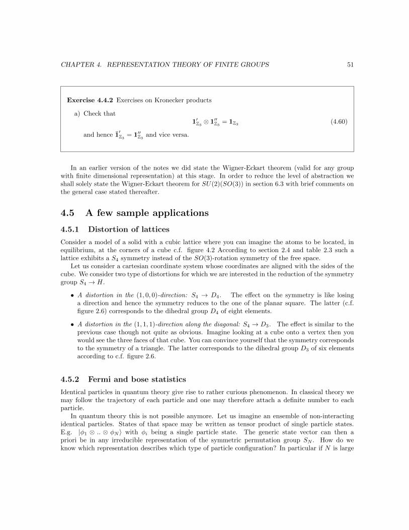
CHAPTER 4. REPRESENTATION THEORY OF FINITE GROUPS 51
Exercise 4.4.2 Exercises on Kronecker products
a) Check that1′Z3⊗ 1′′Z3
= 1Z3(4.60)
and hence 1′Z3
= 1′′Z3and vice versa.
In an earlier version of the notes we did state the Wigner-Eckart theorem (valid for any groupwith finite dimensional representation) at this stage. In order to reduce the level of abstraction weshall solely state the Wigner-Eckart theorem for SU(2)(SO(3)) in section 6.3 with brief comments onthe general case stated thereafter.
4.5 A few sample applications
4.5.1 Distortion of lattices
Consider a model of a solid with a cubic lattice where you can imagine the atoms to be located, inequilibrium, at the corners of a cube c.f. figure 4.2 According to section 2.4 and table 2.3 such alattice exhibits a S4 symmetry instead of the SO(3)-rotation symmetry of the free space.
Let us consider a cartesian coordinate system whose coordinates are aligned with the sides of thecube. We consider two type of distortions for which we are interested in the reduction of the symmetrygroup S4 → H.
• A distortion in the (1, 0, 0)-direction: S4 → D4. The effect on the symmetry is like losinga direction and hence the symmetry reduces to the one of the planar square. The latter (c.f.figure 2.6) corresponds to the dihedral group D4 of eight elements.
• A distortion in the (1, 1, 1)-direction along the diagonal: S4 → D3. The effect is similar to theprevious case though not quite as obvious. Imagine looking at a cube onto a vertex then youwould see the three faces of that cube. You can convince yourself that the symmetry correspondsto the symmetry of a triangle. The latter corresponds to the dihedral group D3 of six elementsaccording to c.f. figure 2.6.
4.5.2 Fermi and bose statistics
Identical particles in quantum theory give rise to rather curious phenomenon. In classical theory wemay follow the trajectory of each particle and one may therefore attach a definite number to eachparticle.
In quantum theory this is not possible anymore. Let us imagine an ensemble of non-interactingidentical particles. States of that space may be written as tensor product of single particle states.E.g. |φ1 ⊗ .. ⊗ φN 〉 with φi being a single particle state. The generic state vector can then apriori be in any irreducible representation of the symmetric permutation group SN . How do weknow which representation describes which type of particle configuration? In particular if N is large
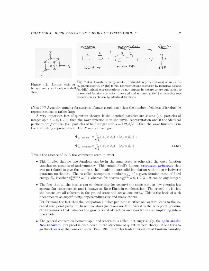
CHAPTER 4. REPRESENTATION THEORY OF FINITE GROUPS 52
Figure 4.2: Lattice with cu-bic symmetry with only one shellshown.
Figure 4.3: Possible arrangements (irreducible representations) of an identi-cal particle state. (right) trivial representations as chosen by identical bosons.(middle) mixed representations do not appear in nature or are equivalent toboson and fermion statistics times a global symmetry, (left) alternating rep-resentation as chosen by identical fermions.
(N ' 1023 Avogadro number for systems of macroscopic size) then the number of choices of irreduciblerepresentations is rather large.
A very important fact of quantum theory: If the identical particles are bosons (i.e. particles ofinteger spin s = 0, 1, 2...) then the wave function is in the trivial representation and if the identicalparticles are fermions (i.e. particles of half integer spin s = 1/2, 3/2...) then the wave function is inthe alternating representation. For N = 2 we have got:
Φ12|bosons =1√2
(|φ1 ⊗ φ2〉+ |φ2 ⊗ φ1〉) ,
Φ12|fermions=1√2
(|φ1 ⊗ φ2〉 − |φ2 ⊗ φ1〉) (4.61)
This is the essence of it. A few comments seem in order:
• This implies that no two fermions can be in the same state as otherwise the wave functionvanishes on grounds of antisymmetry. This entails Pauli’s famous exclusion principle thatwas postulated to give the atomic a shell model a more solid foundation within non-relativisticquantum mechanics. The so-called occupation number nEα of a given fermion state of fixedenergy Eα is either nfermion
Eα= 0, 1 whereas for bosons nboson
Eα= 0, 1, 2, 3, .. it can be any integer.
• The fact that all the bosons can condense into (or occupy) the same state at low energies hasspectacular consequences and is known as Bose-Einstein condensation. The crucial bit is thatthe bosons are all coherent in the ground state and act as one entity. This is the basis of suchphenomenon as superfluidity, superconductivity and many others.
For fermions the fact that the occupation number per state is either one or zero leads to the so-called zero point pressure. In neutronstars (neutrons are fermions) it is the zero point pressureof the fermions that balances the gravitational attraction and avoids the star imploding into ablack hole.
• The general connection between spin and statistics is called, not surprisingly, the spin statis-tics theorem . It’s proof is deep down in the structure of quantum field theory. If one tries togo the other way then one can show (Pauli 1940) that this leads to violation of Einstein causality
CHAPTER 4. REPRESENTATION THEORY OF FINITE GROUPS 53
(commutators of quantum field have support for space-like separation points). The most rigor-ous proof is found in axiomatic quantum field theory (Jost 1957) and uses a complexification(analytic continuation) of the Lorentz symmetry group SO(3, 1).
• In fact at first it might seem somewhat surprising that of the many representation of the symme-try group of SN (for N large) there are only two types which are realised for identical particles.The other representation (mixed representations) were also considered, and referred to as paras-tatistics, but were found to be equivalent to the trivial and alternating representation timesa global symmetry and therefore do not seem to bring in a new element. Note that addingfermions and bosons coherently is not possible because the boson and fermion number is a con-served quantum number. This is known as a superselection rule and will be briefly discussedtowards the end of the course.

CHAPTER 4. REPRESENTATION THEORY OF FINITE GROUPS 54
Exercise 4.5.1 Invariants and mixed representations.
a) The group S4 is generated by
A =
0 1 00 0 11 0 0
, B =
0 0 10 1 01 0 0
, C =
1 0 00 −1 00 0 −1
. (4.62)
Note, in order to check invariance of a potential invariant it is sufficient to check invariancefor a set of group generators. Check that A,B,C both leave I2 = x2 + y2 + z2 I3 = xyzinvariant.
b) Explicit construction of mixed representation We shall construct the standard representationof S3 (which corresponds to a mixed representation) explicitly. The construction is similarto the permutation representation although it is algebraically more involved. This exercisealso contains the seeds to understand the hook formula (4.48) for the Sn.
The representations (4.61) correspond to the trivial and alternating representation of S2:
S2 : 1 : ,1′ :
Let us consider the situation for three particles and construct the mixed representation(parastatistics) of S3:
S3 : 2 :
2 1
3
The representation is two dimensional and the numbers are not the hook lengths but anenumeration to be used below.
The meaning of the arrangement of the boxes for Sn is as follow: First take a vector with ndirections say |φi〉 i = 1..n and then take a tensor product of n of them |φi1⊗..⊗φin〉 and theboxes give the rules of anti(symmetrisation). Indices associated with rows are symmetrisedand indices which are in one column are antisymmetrised over.
Let us implement this on the following state: |φ1 ⊗ φ2 ⊗ φ3〉 (or you can use the notation|φa ⊗ φb ⊗ φc〉 if you find it less confusing) and call the state e1:
e1 = |φ1 ⊗ φ2 ⊗ φ3〉+ |φ2 ⊗ φ1 ⊗ φ3〉 − |φ1 ⊗ φ3 ⊗ φ2〉 − |φ2 ⊗ φ3 ⊗ φ1〉 . (4.63)
A second basis vector might be obtained by starting with |φ1 ⊗ φ3 ⊗ φ2〉
e2 = |φ1 ⊗ φ3 ⊗ φ2〉+ |φ3 ⊗ φ1 ⊗ φ2〉 − |φ1 ⊗ φ2 ⊗ φ3〉 − |φ3 ⊗ φ2 ⊗ φ1〉 . (4.64)
The action of ρstand.(1, 2) = ρ(1, 2) on e1, e2 is then just to interchange labels 1 and 2 (or aand b in the alternative notation).
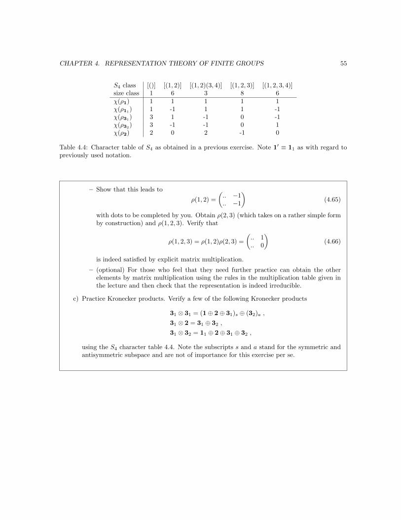
CHAPTER 4. REPRESENTATION THEORY OF FINITE GROUPS 55
S4 class [()] [(1, 2)] [(1, 2)(3, 4)] [(1, 2, 3)] [(1, 2, 3, 4)]size class 1 6 3 8 6χ(ρ1) 1 1 1 1 1χ(ρ11) 1 -1 1 1 -1χ(ρ31) 3 1 -1 0 -1χ(ρ32
) 3 -1 -1 0 1χ(ρ2) 2 0 2 -1 0
Table 4.4: Character table of S4 as obtained in a previous exercise. Note 1′ ≡ 11 as with regard topreviously used notation.
– Show that this leads to
ρ(1, 2) =
(.. −1.. −1
)(4.65)
with dots to be completed by you. Obtain ρ(2, 3) (which takes on a rather simple formby construction) and ρ(1, 2, 3). Verify that
ρ(1, 2, 3) = ρ(1, 2)ρ(2, 3) =
(.. 1.. 0
)(4.66)
is indeed satisfied by explicit matrix multiplication.
– (optional) For those who feel that they need further practice can obtain the otherelements by matrix multiplication using the rules in the multiplication table given inthe lecture and then check that the representation is indeed irreducible.
c) Practice Kronecker products. Verify a few of the following Kronecker products
31 ⊗ 31 = (1⊕ 2⊕ 31)s ⊕ (32)a ,
31 ⊗ 2 = 31 ⊕ 32 ,
31 ⊗ 32 = 11 ⊕ 2⊕ 31 ⊕ 32 ,
using the S4 character table 4.4. Note the subscripts s and a stand for the symmetric andantisymmetric subspace and are not of importance for this exercise per se.

Chapter 5
Lie groups: U(1) ' SO(2),SO(3) ' SU(2)/Z2
Lie groups were discovered by the Norwegian mathematician Sophus Lie (1842-1899) in attemptingto find a Galois theory (solving algebraic equations) for differential equations. Technically theycorrespond to manifolds which are compatible with a group structure. By no means does everymanifold admit a group structure.
In some sense Lie groups are more complicated than finite groups but the classification of thesimple and compact Lie groups due to Cartan and Dynkin is remarkably simple and ingenious at thesame time. The rigidity of the group axioms and the manifold structure are restrictive enough for ashort and concise classification unlike the thousand of research papers that lead to the classification ofsimple finite groups. The key observation is that the linearisation of the Lie group, which correspondsto the so-called Lie Algebra, is sufficient to study many of the properties of the Lie groups. Hencethe apparatus of linear algebra comes into play and allows to make strong statements.
We will only be concerned with the four Lie groups U(1), SO(2), SU(2) and SO(3) which arerelated, as groups as follows:
U(1) ' SO(2) , SO(3) ' SU(2)/Z2 , (5.1)
where the symbol ' stands for isomorphic. In the first section 5.1 we shall, nevertheless, keepthe definitions general so that you can apply them in your further studies to more complicated Liegroups. Lie groups are of major importance in particle physics in term of gauge symmetries (theStandard Model, that is to say the most fundamental theory of particles, has a gauge symmetryU(1)⊗SU(2)⊗SU(3)) or so-called global symmetries (e.g. isospin SU(2) the approximate symmetryunder interchange of up and down quarks).
5.1 Basic definitions
Definition 5.1.1 Continuous group: a continuous group is a group G with an infinite numberof elements which depends continuously on some parameters α ≡ α1, .., αdimG. The number ofcontinuous parameters dimG is known as the dimension of the group.
56
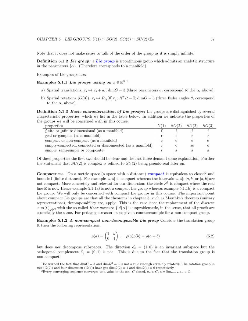
CHAPTER 5. LIE GROUPS: U(1) ' SO(2), SO(3) ' SU(2)/Z2 57
Note that it does not make sense to talk of the order of the group as it is simply infinite.
Definition 5.1.2 Lie group: a Lie group is a continuous group which admits an analytic structurein the parameters α. (Therefore corresponds to a manifold).
Examples of Lie groups are:
Examples 5.1.1 Lie groups acting on ~x ∈ R3 1
a) Spatial translations, xi 7→ xi + ai; dimG = 3 (three parameters ai correspond to the αi above).
b) Spatial rotations (O(3)), xi 7→ Rij(θ)xj ; RTR = I; dimG = 3 (three Euler angles θi correspond
to the αi above).
Definition 5.1.3 Basic characterisation of Lie groups: Lie groups are distinguished by severalcharacteristic properties, which we list in the table below. In addition we indicate the properties ofthe groups we will be concerned with in this course.
properties U(1) SO(2) SU(2) SO(3)finite or infinite dimensional (as a manifold) f f f freal or complex (as a manifold) r r r rcompact or non-compact (as a manifold) c c c csimply-connected, connected or disconnected (as a manifold) c c sc csimple, semi-simple or composite s s s s
Of these properties the first two should be clear and the last three demand some explanation. Furtherthe statement that SU(2) is complex is refined to SU(2) being pseudo-real later on.
Compactness On a metric space (a space with a distance) compact is equivalent to closed2 andbounded (finite distance). For example [a, b] is compact whereas the intervals [a, b[, ]a, b] or ]a, b[ arenot compact. More concretely and relevant for our discussion: the circle S1 is compact where the realline R is not. Hence example 5.1.1a) is not a compact Lie group whereas example 5.1.1b) is a compactLie group. We will only be concerned with compact Lie groups in this course. The important pointabout compact Lie groups are that all the theorems in chapter 3, such as Maschke’s theorem (unitaryrepresentations), decomposability etc, apply. This is the case since the replacement of the discretesum
∑g∈G with the so called Haar measure
∫dα is unproblematic, in the sense, that all proofs are
essentially the same. For pedagogic reason let us give a counterexample for a non-compact group.
Examples 5.1.2 A non-compact non-decomposable Lie group Consider the translation groupR then the following representation,
ρ(a) =
(1 a0 1
), ρ(a)ρ(b) = ρ(a+ b) (5.2)
but does not decompose subspaces. The direction ~ex = (1, 0) is an invariant subspace but theorthogonal complement ~ey = (0, 1) is not. This is due to the fact that the translation group isnon-compact!
1Be warned the fact that dimG = 3 and dimR3 = 3 is not a rule (though certainly related). The rotation group intwo (O(2)) and four dimension (O(4)) have got dimO(2) = 1 and dimO(4) = 6 respectively.
2Every converging sequence converges to a value in the set: C closed, an ∈ C, a = limn→∞ an ∈ C.

CHAPTER 5. LIE GROUPS: U(1) ' SO(2), SO(3) ' SU(2)/Z2 58
Connectedness A set is connected if there is a smooth path from each point of the set to anyother point of the set. It is in particular simply connected if all loops can be contracted in a smoothfashion to a point. A set which is not connected is disconnected. In Fig. 5.1 three illustrative andhopefully clarifying examples are given. We shall only be concerned with connected Lie groups. We
Figure 5.1: (left) simply connected set (middle) connected set which is not simply connected (right) discon-nected set
will briefly discuss an example of a non-connected group in the next chapter in example 5.2.1 so thatyou will get an idea of what is going on. The fact that SU(2) is simply connected and SO(3) onlyconnected is related to the existence of fermions.
Simplicity A simple Lie group is a connected non-abelian Lie group which does not admit (non-trivial) connected normal subgroups. This connects to the definition of a simple group for finitegroups. Similarly simple Lie groups are the atoms of Lie group since no (Lie) quotient groups can bedefined. Semi-simple Lie groups are direct products of simple Lie groups. Composite Lie groups arecomposed of simple Lie groups through semi-direct products or more complicated operations and arebeyond the scope of this course. We shall only be concerned with simple Lie groups3 in this course.
Some examples of simple and compact Lie groups used in physics are:
Examples 5.1.3 Examples of finite, simple and compact Lie groups are:
- Special orthogonal groups are real.4
SO(n) = O ∈ GL(n,R) | OTO = In ,detO = 1 (5.3)
- Special unitary groups are complex.
SU(n) = U ∈ GL(n,C) | U†U = In ,detU = 1 (5.4)
- Symplectic groups are complex.
USp(2n) ≡ Sp(n) = S ∈ GL(2n,R) | STJS = J , J =
(0 In−In 0
) (5.5)
play a role in Hamiltonian dynamics. Note J2 = −I2n and hence J is in some sense a squareroot of minus one.
3Including the abelian Lie groups in the simple category.4The S-denotes the determinant condition.

CHAPTER 5. LIE GROUPS: U(1) ' SO(2), SO(3) ' SU(2)/Z2 59
G dim rank
An [SU(n+ 1)] (n+ 1)2 − 1 nBn [SO(2n+ 1)] (2n+ 1)n nCn [USp(2n)] n(2n+ 1) nDn [SO(2n)] n(2n− 1) n
E6 78 6E7 133 7E8 248 8F4 52 4G2 14 2
Table 5.1: Dimension and rank (which is the dimension of the Lie Algebra, c.f. section 5.3) of simple andcompact Lie groups. The so-called exceptional groups E6,7,8, F4 and G2 are mentioned for completeness onlyand do not play any role in the remainder of the course. They are called exceptional because they do not fallinto any of four first series. The corresponding Dynkin diagrams are shown on the right for completeness onlywithout any in depth explanation other than the remark that the number of circles corresponds to the rank.Symmetries can be inferred from the Dynkin diagrams. For example some types of low ranks are degenerate.E.g. A1 ' B1 (SU(2) ' SO(3) which is relevant for the course). Or D2 ' A1⊕A1 (SO(4) ' SU(2)⊗SU(2))which is the only example of a semi-simple type in this list.
The groups U(n) and O(n) are the same as SU(n) and SO(n) except that the determinant conditionis not imposed. (The “S” stands for special). A relation between the two is given in (5.17) lateron. The classification of the simple compact Lie groups has been done by Cartan and Dynkin and isastonishingly beautiful and simple. The study of which is beyond the scope of this course. In table 5.1we have listed all groups for the sake of completeness. The dimension of the defining representations(5.3,5.4,5.5) is given in the middle column and the rank (to be defined in section 5.3) is given in theright column. For pedagogical reason let us give an example of a non-compact Lie group of importancein physics:
Examples 5.1.4 The Lorenzt-group SO(3, 1): a non-compact Lie group
SO(3, 1) = Λ ∈M4(R) | ΛT ηΛ = η ,det Λ = 1 , η = diag(1,−1,−1,−1) . (5.6)
A way to see that they are not compact is to note that they contain the boost to any reference frameof relative speed v ∈ [0, c[ where c is the speed of light. This is a non-compact interval and thereforeSO(3, 1) cannot be a compact group.5
Much of the power of Lie groups relies on the realisation that, for many aspects, it is sufficientto linearise the problem in the parameters α mentioned earlier. By linearising one departs fromthe Lie group to the Lie Algebra which may be thought of as the tangent space of the manifold.By exponentiating the Lie Algebra elements one gets back the connected part of the Lie group (bywhich we mean the part connected to the identity). These concepts will be illustrated through thesimple example of U(1) in the next section. The end this introduction with the following mnemonic:
Linearisation: Lie group ⇒ Lie Algebra ,
Exponentiation: Lie Algebra⇒ connected part of Lie group (5.7)
5One consequence of this fact is that there do not exist any finite dimensional unitary representations of the Lorentzgroup. (For the experts: this is why Ψ = Ψ†γ0 is necessary to define invariant of the form ΨΨ where Ψ is a spinor.)

CHAPTER 5. LIE GROUPS: U(1) ' SO(2), SO(3) ' SU(2)/Z2 60
Exercise 5.1.1 Generalities on compact simple Lie groups
a) Check that the dimension of the matrices SO(n) and SU(n) are indeed n2−1 and n(n−1)/2in accordance with table 5.1.Hint: Use the fact that U = exp iH and O = exp iA where H and A are hermitian tracelessand antisymmetric respectively. Note an arbitrary Mn(C)-matrix has got 2n2 parameters.
b) Using the formula det(exp(tr[A])) = exp(tr[A]) check that the determinant condition issatisfied if H from the previous exercise are traceless.
5.2 The two abelian groups: U(1) and SO(2)
The groups U(1) and SO(2) can be defined as:
U(1) = z ∈ C | |z| = 1 , SO(2) = O ∈M2(R) | OTO = I2, det(O) = 1 . (5.8)
They are rather simple, as abelian groups tend to be, and in particular isomorphic to each other.They correspond to an angle of rotation around 2π. Representation matrices are given by
ρn(α)|U(1) = einα , ρn(α)|SO(2) =
(cos(nα) sin(nα)− sin(nα) cos(nα)
), n ∈ Z , α ∈ [0, 2π[ (5.9)
which makes the isomorphism U(1) ' SO(2) explicit. Intuitively they correspond to rotation arounda single axis. All irreducible representations of U(1) are given by one dimensional representation onC. The irreducible representations of SO(2) are given by two dimensional representations on R2.Note that the cyclic groups Zk are finite subgroups of U(1). The Kronecker product (Clebsch-Gordanseries) of two representations is given by
U(1) : ρn ⊗ ρm = ρn+m (5.10)
for U(1) (and therefore for SO(2) as well.)In principle we could end here but we consider it useful to illustrate the notions of exponentiation,
Lie Algebra and connectedness in this simplified context. Let us make the following ansatz forO ∈ SO(2)6
O = exp(iαT ) , T ∈M2(R) , (5.11)
where the exponential map of matrices can be understood in the sense of a power series or any otherwell known limiting process
exp(A) =∑n≥0
An
n!= limn→∞
(1 +
A
n
)n. (5.12)
6Mathematicians often omit the factor of i in the exponential and absorb it into the generator. This is in someways more convenient as you will notice. We will stick to the convention below which is the one adopted in the physicsliterature.

CHAPTER 5. LIE GROUPS: U(1) ' SO(2), SO(3) ' SU(2)/Z2 61
The exponential has the following property: det(exp(A)) = exp(Tr(A)) which can be shown byconsidering the eigenvalue expression of the determinant and the trace.
Note that the defining condition (5.9) (using exp(A)T = exp(AT ) which follows from (5.12))
I2 = OTO = exp(iαTT ) exp(iαT )) = I2 + iα(TT + T ) +O(α2) ⇔ TT = −T , (5.13)
implies that T has got to be an antisymmetric matrix and this condition immediately generalises toSO(n).7 The following matrix,
T = −i(
0 1−1 0
), T 2 = I2, eiαT = I2 cos(α) + iT sin(α) = ρ(α)SO(2) , (5.14)
leads to the representation (5.9). The generator T emerges from the linearisation of eiαT = 1 +iαT +O(α2). In the case at hand the Lie Algebra is rather trivial since it has only a single element Tand no further structure. Nevertheless it serves us well in illustrating or hinting at the connection withdifferential geometry in terms of manifolds (surfaces correspond to manifolds in two dimensions). InFig. 5.2 we illustrate the manifold nature of SO(2) and its tangent space. It is meant as an illustrationonly and is of no importance for the rest of the course other than broadening the viewpoint.
Figure 5.2: SO(2)-manifold S1 embedded into R2. (S1 corresponds to a circle). Shown are two maps fromintervals on R which cover the manifolds. An explicit realisation of f1 is given by f1(θ) = (cos(θ), sin(θ) forexample. It is explicitly seen that T , the (Lie Algbra) generator of SO(2), corresponds to the tangent vector.Illustrated for (x, y) = (−1, 0) (in green) which leads to T (−1, 0) = (0,−1).
Another element which wish to illustrate is (dis)connectedness.
Examples 5.2.1 O(2): A disconnected Lie group. The manifold SO(2) is connected as can beseen from the figure but O(2) is not. Note that det(O) = ±1 follows from OTO = I2. Since O isdifferentiable, one cannot go in a continuous fashion from a point in the set det(O) = 1 to a point of
7Note the last step on the left hand side in (5.13) is only valid if T commutes with its transpose as otherwise theBaker–Campbell–Hausdorff formula (to be discussed soon) has to be applied. Since T is an antisymmetric matrix itdoes commute with its transpose and so the steps are finally consistent.
CHAPTER 5. LIE GROUPS: U(1) ' SO(2), SO(3) ' SU(2)/Z2 62
the set detO = −1 and hence O(2) is not connected.8 For example
P =
(1 00 −1
), P ∈ O(2) , P /∈ SO(2) (5.15)
is an example of a matrix which is in O(2) but not in SO(2). One may think of P as a parity operator.In fact P generates the cyclic group Z2 which is a normal subgroup9 of O(2) and the following relationholds:
SO(2) ' O(2)/Z2 , (5.16)
and slightly more generally
SO(n) ' O(n)/Z2 , SU(n) ' U(n)/U(1) . (5.17)
The symbol ' stands for isomorphic.
It seems worthwhile to pause for a moment and try to reconnect to the chapter of finite groups.First we note that there ought to be, in general, an infinite amount of irreducible representations byvirtue of a limiting process of the dimensionality theorem 4.1.2 (|G| → ∞ implies infinitely manyirreducible representations in Eq. (4.19)). For U(1) the series is given in Eqs. (5.9). For U(1) theHaar measure.10 is rather simple. An inner product is defined as follow11:
〈χn|χm〉|U(1) ≡∫ 2π
0
dα
2πχ(ρn(α))∗χ(ρm(α)) =
∫ 2π
0
dα
2πeiα(m−n) = δmn , (5.18)
under which the χn are orthonormal. The characters will not play a pivotal role in the analysis of ofthe representations as we will find that the so-called highest weight representations of Lie Algebra tobe a powerful tool to construct representations.
Exercise 5.2.1 U(1) and SO(2)
a) Check that ρn(α1)SO(2)ρn(α2)SO(2) = ρn(α1 + α2)SO(2) using the representation (5.9).Trigonometric identities can easily derived using Euler’s formula eia = cos(a) + i sin(a).
b) Using Euler’s formula verify (5.14).
c) Conceptual question: what would happen in case n is not chosen to be an integer in (5.9)?
8If one were to complexify the group which merely amounts to allow for complex α then the determinant would takeon any complex value and one could go from any point to another in a continuous fashion. Hence the complexificationof O(2) is connected. This general knowledge is encapsulated in Jacques Hadamard’s (1865-1963) famous quote: “theshortest path between two truths in the real domain passes through the complex domain”.
9In particular any abelian subgroup is normal. Hence Z2, which is abelian, is normal.10The Haar measure generalises 1
|G|∑g∈G from finite groups.
11The second orthogonality relation becomes 〈χ[α]|χ[α′]〉C |U(1) = 12π
∑n∈Z e
in(α−α′) = δ(α−α′) for α, α′ ∈ [0, 2π[.

CHAPTER 5. LIE GROUPS: U(1) ' SO(2), SO(3) ' SU(2)/Z2 63
5.3 Some generalities of (non-abelian) simple compact Liegroups
In this section we would like to clarify and elaborate on the aspect of the necessity of the exponentialmap and the structure of the Lie Algebra. The exponentiation of the latter gives rise to the groupstructure.
Theorem 5.3.1 exponential mapEach one-parameter subgroup of GL(n,C) is given by a matrix exponential ρT (t) = exp(tT ) whereT ∈Mn(C) 6= 0 is the generator.
Proof: Consider a one-parameter homomorphism ρT (t) : R→ GL(n,C) defined by:
d
dtρT (t)|t=0 = T , (5.19)
with boundary condition ρT (0) = I. Since ρT is a group homomorphism
ρT (s+ t) = ρT (s)ρT (t) . (5.20)
Differentiating w.r.t. to s and setting s = 0, leads to
d
dtρT (t) = TρT (t) ⇒ ρT (t) = exp(tT ) , (5.21)
a first order linear differential equation with unique solution as indicated q.e.d.
Next we want to explore what constraints the group axioms impose on the structure of the gen-erator T in general. Higher dimensional groups are parameterised by several parameters as discussedat the beginning of the chapter (e.g. the three-dimensional rotation group SO(3) is described by thethree Euler angles.). Motivated by the exponential form we start with the following ansatz:
ρ1 = I + iαaTa +1
2(iαaTa)2 +O(α3) ,
ρ2 = I + iβbTb +1
2(iβbTb)
2 +O(β3) ,
ρ3 = I + iγcTc +1
2(iγcTc)
2 +O(γ3) , (5.22)
where summation over repeated indices a, b and c is understood a = 1..dLA. (In the case of SO(3),αa correspond to the three Euler angles.) Further we note that the precoefficient of the quadraticterm follows from ρ(α)2 = ρ(2α) which in turn derives from (5.20) or generally from theorem 5.3.1.The matrices Ta are the Lie Algebra generators.
Multiplication of two exponential of matrices is different from normal multiplication of two expo-nentials exp(a) exp(b) = exp(a+ b) for a, b ∈ C in that the two matrices do not necessarily commute.The formula governing the arithmetics is the famous Baker–Campbell–Hausdorff formula :
eAeB = eA+B+ 12
[A,B]+ 13!
12
([A,[A,B]]+[[A,B],B])+··· , (5.23)

CHAPTER 5. LIE GROUPS: U(1) ' SO(2), SO(3) ' SU(2)/Z2 64
where [A,B] = AB−BA denotes the commutator. In order to assess the structure of the Lie Algebrawe are going to investigate under what conditions
ρ3 = ρ1ρ2ρ−11 ρ−1
2 , (5.24)
is consistent with the linear ansatz in (5.22). Eq. (5.24) can be considered as the definition of theelement ρ3 for instance. In order to determine the conditions on the αa, βb, γc’s we substitute (5.22)into (5.24) which leads to
[αaTa, βbTb] = −iγcTc +O(α3, β3, γ3) , (5.25)
where all lower order terms cancel. The solution is given by γc = −f cab α
aβb provided that thegenerators satisfy the so-called Lie Algebra
Generic Lie Algebra: [Ta, Tb] = if cab Tc . (5.26)
Summation over c is again understood and f cab are known as the structure constants of the Lie
Algebra which are in particular antisymmetric in the indices a and b. This answers the question whatkind of structure the generators have to satisfy in order to be compatible with the group structure.Crucially the Lie Algebra only depends on the commutator, as is inherent in the Baker–Campbell–Hausdorff formula (5.23), and not on the anti-commutator. The latter depends on the representationof the Lie Algebra.12
An important notation is the rank of a Lie Algebra , which is the maximal number of Lie Algebragenerators that commute with each other (and not to be confused with the dimension of the LieAlgebra dLA ≥ rank). For the simple compact groups this number is indicated in table 5.1 on theright hand side and corresponds to the number of dots in the Dynkin diagrams. Its instrumental inconstructing the representations. Note, the rank of SO(3) and SU(2) is one. Hence they are thesimplest non-abelian Lie groups but nevertheless rich enough to keep us busy until the end of thecourse! We note that the matrix T (5.14) plays, the slightly degenerate, role of the Lie Algebra ofSO(2).
Theorem 5.3.2 Lie Algebra ↔ unique simply connected Lie groupTo each given Lie Algebra corresponds a unique Lie Group which is simply connected. This group is
known as the universal covering group.13
We will not present the proof. The impotent point is that for identical Lie Algrabra’s correspond ingeneral several Lie groups. Only under the restriction to simply connectedness the exponential mapis 1-to-1 (bijective). The other not simply connected groups can be obtained as quotient groups.
Theorem 5.3.3 Lie Algebra generators of a compact group are hermitianFor compact Lie groups there exist a Lie Algebra basis where the generators are hermitian (T †a = Ta).
Proof: (sketch) The part connected to the identity matrix can be written as ρ = exp(iαaTa) andsince compact groups admit finite dimensional unitary representations,
In = exp(iαaTa)† exp(iαaTa) = exp(−iαaT †a ) exp(iαaTa) (5.27)
= In + iαa(Ta − T †a ) +O(α2) ⇔ T † = T , (5.28)
expansion in the parameter α-reveals the condition.
12For SU(2) the anti-commutator vanishes for all representations and is related to the fact that SU(2) is of rank one.13A term which derives from the field of topology.

CHAPTER 5. LIE GROUPS: U(1) ' SO(2), SO(3) ' SU(2)/Z2 65
Corollary 5.3.1 The Hilbert-Schmidt inner product on Mn(C) assumes the form
〈Ta|Tb〉 ≡ Tr[T †aTb]thm 5.3.3
= Tr[TaTb] . (5.29)
Theorem 5.3.4 For compact, semi-simple Lie algebras there exists an orthogonal basis,
〈Ta|Tb〉 = Tr[TaTb] = 2kRδab . (5.30)
The number kR is the called the Dynkin index and depends on the representation (hence thesubscript R). In this basis (5.30) the structure constants f c
ab = fabc are completely antisymmetric inall three indices (c.f. box below).
We shall omit the proof. Below we give a slightly more precise statement which is though beyond thescope of this course and targeted at the interested reader only. Yet we shall use the result as a matterof convenience to lower all indices.14
for the interested reader (not part of the course)
Theorem 5.3.5 Killing metricOne can define a unique symmetric tensor (Killing metric)
Tr[TaTb] = kRkab , (5.31)
invariant under the action of the Lie group
0 = δTcTr[TaTb] = Tr[[Tc, Ta]Tb] + Tr[Tb[Tc, Tb]] = 2ikR(f bca + f a
cb ) . (5.32)
The number kR is the Dynkin index which is dependent on the representation. Note the(complete) antisymmetry of f c
ab follows from the invariance of the killing metric (5.32).For semi-simple Lie groups the killing metric is non-singular and if in addition the group iscompact then there exists a basis where
kab = 2δab . (5.33)
Proof omitted. Note the Killing metric can be used to lower and raise indices. Since forsemi-simple groups the Killing metric is the identity matrix we shall take a rather relaxedattitude towards upper and lower indices.
Theorem 5.3.6 General properties of structure constants fabc for Lie groupsThe structure constant satisfy the Jacobi identity :
faedfbce + fbedfcae + fcedfabe = 0 . (5.34)
Proof: (sketch) Any three matrices A,B,C satisfy (exercises):
[A, [B,C]] + [B, [C,A]] + [C, [A,B]] = 0 , (5.35)
14For semi-simple but non-compact groups the metric 〈Ta|Tb〉 = kab is non-degenerate and can be used to lowerindices.

CHAPTER 5. LIE GROUPS: U(1) ' SO(2), SO(3) ' SU(2)/Z2 66
and so does(T adja )bc = ifabc , (5.36)
interpreted as a matrix q.e.d.The label adj(oint) is explained in the preceding corollary.
Corollary 5.3.2 The adjoint representation is real
a) Eq. (5.36) defines a representation called the adjoint representation .15
b) The structure constants are real. (fabc ∈ R)
Proof: The show that (5.36) is a representation is left as an (optional) exercise. Reality of fabc canbe seen as follows. If Ta generates a representation of the Lie Algebra so does (−T ∗a ), the complexconjugate representation.16 By Taking the complex conjugate of (5.26) one gets:
[−T ∗a ,−T ∗b ] = if∗abc(−T ∗c ) . (5.37)
Since the complex conjugate corresponds to the same group this implies f∗abc = fabc q.e.d.
Exercise 5.3.1 Generalities on compact simple Lie groups
a) Check that Eq. (5.35) is correct for any set of matrices.
b) Check that ρ(α)2 = ρ(2α) and ρ(α)−1 = ρ(−α) using equations in the proof of theorem5.3.1.
c) Verify Eq. (5.25).
d) (optional) Using the Jacobi identity (5.34) show that (5.36) is indeed a Lie Algebra repre-sentation of the form (5.26).
5.4 The two non abelian groups: SU(2) and SO(3)
5.4.1 Lie Algebras of SO(3) and SU(2)
After the preparatory steps of the preceding chapter it is not difficult to write down the Lie Algebraof SO(3) (usually denoted by so(3) lower case letters). From exercise 5.1.1 we know that any threelinearly independent antisymmetric matrices will generate the algebra. A basis for which the structureconstant is completely antisymmetric, which is a possibility according to theorem 5.3.4, is given by:
T1 = −i
0 0 00 0 10 −1 0
, T2 = −i
0 0 −10 0 01 0 0
, T3 = −i
0 1 0−1 0 00 0 0
. (5.38)
15The adjoint representation is reminiscent of the regular representation in that the element of the set are declaredto be linearly independent vectors defining a vector space. The adjoint representation acts on the vector space of the
Lie Algebra as follows: (T adja )Td = [Ta, Td] = ifadeTe.
16The minus sign originates from the factor i in the parameterisation exp(iαaTa) of Lie group elements.

CHAPTER 5. LIE GROUPS: U(1) ' SO(2), SO(3) ' SU(2)/Z2 67
The first two indices of T3 are equal to the SO(2) rotation T in (5.14) and corresponds to a rotationaround the z-axis. The remaining T1,2 are just permutations thereof. The Lie Algebra is readilycomputed to be
Lie Algebra: [Ta, Tb] = iεabcTc , (5.39)
where the structure constant fabc = εabc is the completely antisymmetric Levi-Civita tensor (ε123 = 1).In accordance with theorem 5.3.6 the structure constant is real and totally antisymmetric as claimedabove. From Tr[TaTb](5.38) = 2δab, (kR)(5.38) = 1 by (5.30).
The Lie Algebra of SU(2) does not follow, at least in the first instance, in such a geometric manner.We know though that the Lie Algebra generators of SU(n) are hermitian and traceless matrices(according to exercise 5.1.1). The group SU(2) is of dimension three and the three generators can bechosen to be
(Ta)SU(2) =σa2, (5.40)
proportional to the famous Pauli matrices
σ1 =
(0 11 0
)σ2 =
(0 −ii 0
)σ3 =
(1 00 −1
). (5.41)
This implies that (5.40) satisfies the Lie Algebra (5.39). Yet Tr[TaTb](5.40) = 1/2δab and hence theDynkin index (kR)(5.40) = 1/4. What is going on? This means that the Lie groups SU(2) and SO(3)are locally isomorphic (same Lie Algebra) but are globally different (unequal Dynking index). Thisis indeed possible as they are of the same rank; namely of rank one. By virtue of theorem 5.3.2 thereis a unique simply connected Lie group associated with each Lie Algebra. In the case at hand this isSU(2) as we wish to demonstrate. Consider the mapping from R4 → SU(2):
φ : (x0, x1, x2, x3) = x0I2 + x1iσ1 + x2iσ2 + x3iσ3 =
(x0 + ix3 ix1 + x2
ix1 − x2 x0 − ix3
)= U (5.42)
The two defining conditions of SU(2) lead to:
UU† = I2 , detU = 1 ⇔ x20 + x2
1 + x22 + x2
3 = 1 . (5.43)
It follows that SU(2) is topologically equivalent to the three sphere S3. The latter is simply connectedand therefore SU(2) is the unique simply connected Lie group corresponding to the Lie Algebra (5.39).Hence if SO(3) is not identical to SU(2), which it is clearly not, then there must exist a n-to-1homomorphism from SU(2) to SO(3). The latter is given by the so-called Weyl-homomorphism
h(~x) = x1σ1 + x2σ2 + x3σ3 , (5.44)
which obeysUh(~x)U† = h(O~x) , U = eiα
a(Ta)SU(2) , O = eiαa(Ta)SO(3) . (5.45)
Hence the Weyl homomorphism is a 2-to-1 map ρSU(2) → ρSO(3) : U → O. The kernel of thishomomorphism is given by ±I ' Z2 and by virtue of the first isomorphism theorem 2.2.8 thefollowing isomorphism holds
SO(3) ' SU(2)/Z2 . (5.46)
We note that SO(3) is not simply connected since SU(2) is the unique simply connected Lie groupassociated to (5.39). This has profound implications and is related to the existence of fermions as weshall see.
CHAPTER 5. LIE GROUPS: U(1) ' SO(2), SO(3) ' SU(2)/Z2 68
Exercise 5.4.1 SO(3) and SU(2) Lie algebra
a) Verify that (5.40), (5.38) satisfy the Lie Algebra (5.39).
b) Verify that the representations in a) satisfy (5.30) with kR = (1/4, 1) respectively.
5.4.2 Irreducible representations of SU(2) (and hence SO(3))
In view of the 2-to-1 Weyl homomorphism it is sufficient to construct the irreducible representationsof SU(2) from which the irreducible representations of SO(3) will follow. We shall apply the verygeneral method of highest weight representation which can be applied to any of the Lie Algebra’s of thegroups given in table 5.1. The complication raises with the rank. of the irreducible representations.In fact to each r = rank is associated a so-called Casimir operator which is an operator constructedfrom the Lie Algebra element which commutes with the Lie Algebra. Irreducible representations arelabeled by r labels.
The group SU(2) is of rank one and has therefore got one Casimir operator. In this section weshall denote, because of reasons of familiarity, the generators of the SU(2) Lie Algebra by
Ja ≡ Ta of Eq. (5.39) (5.47)
The quadratic Casimir operator, for any Lie group, is given by T 2 ≡ kabTaTb (with summation overindices a and b understood); when applied to SU(2) one gets:
J2 = J21 + J2
2 + J23 , [J2, Ji] = 0 (5.48)
in the basis (5.31). The Casimir operator is of the form,
J2 = C2(R)IdimVR , (5.49)
by virtue of Schur’s lemma! The eigenvalue C2(R) (which will be identified by j(j+1) latter on) servesto label the irreducible representation. As a set of maximally commuting operators we choose,17
J2, J3 . (5.50)
The eigenvalue of J3, denoted by m, labels the states in a given irreducible representation:
J3em = mem , m ∈ R , (5.51)
where em denotes a basis state in a given representation. From the Lie Algebra the following algebraicrelations are immediate:
[J3, J±] = ±J± , J± ≡ J1 ± iJ2 ((J±)† = J∓) (5.52)
J2 = J23 + J3 + J−J+ , (5.53)
J2 = J23 − J3 + J+J− . (5.54)
17In a quantum system that exhibits rotational symmetry, one would add the Hamiltonian to this set of commutingobservables. Here we try to extract the group theoretic aspects only.
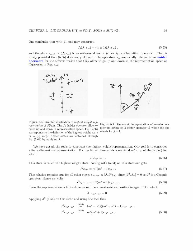
CHAPTER 5. LIE GROUPS: U(1) ' SO(2), SO(3) ' SU(2)/Z2 69
One concludes that with J± one may construct,
J3(J±em) = (m± 1)(J±em) , (5.55)
and therefore em±1 ∝ (J±em) is an orthogonal vector (since J3 is a hermitian operator). That isto say provided that (5.55) does not yield zero. The operators J± are usually referred to as ladderoperators for the obvious reason that they allow to go up and down in the representation space asillustrated in Fig. 5.3.
Figure 5.3: Graphic illustration of highest weight rep-resentation of SU(2). The J± ladder operator allow tomove up and down in representation space. Eq. (5.56)corresponds to the definition of the highest weight statem = j(−m∗). Other states are obtained throughEq. (5.69) by applying J−.
Figure 5.4: Geometric interpretation of angular mo-mentum acting on a vector operator v1i where the onestands for j = 1.
We have got all the tools to construct the highest weight representation. Our goal is to constructa finite dimensional representation. For the latter there exists a maximal m∗ (top of the ladder) forwhich
J+em∗ = 0 . (5.56)
This state is called the highest weight state. Acting with (5.53) on this state one gets
J2em∗ = m∗(m∗ + 1)em∗ . (5.57)
This relation remains true for all other states em∗−n ∝ (J−)nem∗ since [J2, J−] = 0 as J2 is a Casimiroperator. Hence we write
J2em∗−n = m∗(m∗ + 1)em∗−n . (5.58)
Since the representation is finite dimensional there must exists a positive integer n∗ for which
J−em∗−n∗ = 0 . (5.59)
Applying J2 (5.54) on this state and using the fact that
J2em∗−n∗(5.54)
= (m∗ − n∗)((m∗ − n∗)− 1)em∗−n∗ ,
J2em∗−n∗(5.58)
= m∗(m∗ + 1)em∗−n∗ , (5.60)
CHAPTER 5. LIE GROUPS: U(1) ' SO(2), SO(3) ' SU(2)/Z2 70
once concludes that2m∗ = n∗ ∈ Z+ , (5.61)
the irreducible representations are labelled by half-integer.Going over to more standard notation we choose j ≡ m∗ and denote the state vectors by
em → |j,m〉 , (5.62)
where we have introduced in addition the letter j which labels the irreducible represenation. Insummary the irreducible representations of SU(2) are labelled by half integer j and they are (2j + 1)dimensional with m ranging from m = −j,−(j − 1), .., (j − 1), j.
In particular we conclude that the SO(3) representation (5.38) corresponds to j = 1 (note (2 · (j =1) + 1) = 3 is three dimensional) and the SU(2) representation (5.40) corresponds to j = 1/2.Hence (5.40) is the smallest irreducible representation for SU(2) and (5.38) is the smallest irreduciblerepresentation of SO(3). The matrix elements of the highest weight representation are given by:(
J(j)3
)mm′
= 〈j,m|J3|j,m′〉 = mδmm′ , (5.63)(J
(j)±
)mm′
= 〈j,m|J±|j,m′〉 = N±(j,m)δm,m′±1 , (5.64)
with normalisation factor
N±(j,m) ≡ [(j ∓m)(j ±m+ 1)]1/2
= [j(j + 1)−m(m± 1)]1/2
. (5.65)
The equations above fully specify the representations of the algebra. The representation ρ themselvesare given by
ρj(~α)mm′ = 〈j,m|eiαaTa |j,m′〉 , (5.66)
which connects us back to the way we have been handling representations for finite groups. Note jdenotes the representation, α “enumerates” the group elements and m,m′ parameterise the (2j+1)×(2j+1)-dimensional matrix in the so-called highest weight representation. A specific parameterisation,
Dj(α, β, γ)mm′ = 〈j,m|e−iαJze−iβJye−iγJz |j,m′〉 ≡ e−i(mα+m′γ)dj(β)mm′ (5.67)
is known as the Wigner D-matrix (djmm′(β) is sometimes called the little Wigner D-matrix). Itis widely used in the literature and ties in nicely with calculation of angular decay distributionamplitudes. Note Jx does not need to be parameterised since it is implicitly generated throughcommutators of Jy and Jz.
The quadratic Casimir and the Dynkin index are given by:
C2(j) = j(j + 1) , kj = j(j + 1)(2j + 1)
6, (5.68)
where the first equation follows from (5.58) with m∗ = j and the second one is left as an exercise.
Exercise 5.4.2 Irreps of SU(2)

CHAPTER 5. LIE GROUPS: U(1) ' SO(2), SO(3) ' SU(2)/Z2 71
a) Derive Eqs. (5.52,5.53,5.54) using the commutation relations (5.39).
d) Verify the eigenvalue equation for the ladder states in Eq. (5.55).
c) Prove that (5.65) is the correct normalisation factor of
J±|j,m〉 = N±(j,m)|j,m± 1〉 , (5.69)
up to an absolute value. Hint: You may want to use: (5.53) or (5.54) in doing so as well asthe completeness relation in I2j+1 =
∑m |j,m〉〈j,m|.
d) Obtain Jx,y,z from Eqs. (5.63,5.64) for j = 1. Check that [Jx, Jy] = iJz by explicit matrixmultiplication. How do the rotation matrices compare with (5.38)?
e) (optional)
– Take the trace of the Casimir
T 2 = δabTaT b = C2(R)IdimVR (5.70)
to establish18
2kR dimVadj = C2(R) dimVR . (5.71)
– For SU(2) establish (5.68):
kj = j(j + 1)(2j + 1)
6(5.72)
and hence (k1/2, k1, k3/2, ..) = (1/4, 1, 3/2, ..). Hint: C2(j) = j(j+1), dimVj = (2j+1),dimVadj
= dimV1= 3. Make sure you understand all the equations in the hint.
5.4.3 Clebsch-Gordan series of SU(2)
From your course on quantum mechanics you know that when two particles of angular momentum j1and j2 are combined then the total angular momentum ranges from |j1−j2| to j1 +j2 in integer steps.The addition of angular momentum corresponds to taking tensor product representations of states19.The product on the level of the group corresponds by virtue of the exponential map to addition atthe level of the Lie Algebra.
Theorem 5.4.1 The Clebsch-Gordan series for SU(2) (or Kronecker product) is given by
ρj1 ⊗ ρj2 = ρ|j1−j2| ⊕ ρ|j1−j2|+1 ⊕ ...⊕ ρj1+j2 =
j1+j2⊕J=|j1−j2|
ρJ . (5.73)
where two representations ρj are in an irreducible representation with Casimir value j(j + 1).
19Strictly speaking one assumes, in this simplified line of argument, that the mutual interaction will not change thispicture. In fact it doesn’t. The explanation of which is beyond the scope of this course.
CHAPTER 5. LIE GROUPS: U(1) ' SO(2), SO(3) ' SU(2)/Z2 72
A few explanations are in order. We see that the multiplicity of each representation is one whichimplies that SU(2) is a simply reducible group (c.f. definition 6.3.2) as stated earlier on. A non-trivial check of this formula is given by matching up the dimensions,
(2j1 + 1)(2j2 + 1) = (2|j1 − j2|+ 1) + (2(|j1 − j2|+ 1) + 1) + ...(2(j1 + j2) + 1) , (5.74)
which is left as an exercise. A more substantial proof, from which we will use some results later on,is given below.
Proof: Let us compute the character of a Wigner rotation matrix. First consider a rotation around asingle angle. This is in fact sufficient since any other rotation is equivalent by similarity transformationand has therefore identical character. Let us choose (α, β, γ) = (θ, 0, 0) for which the rotation matrix(5.67) is diagonal:
Dj(θ, 0, 0)mm′ = e−imθδmm′ . (5.75)
From (5.75) one obtains (last step is left as an exercise):
χ(ρj(θ)) ≡ χj(θ) =
j∑m=−j
(Dj(θ, 0, 0)
)mm
=
j∑m=−j
eimθ = e−ijθ2j∑m=0
(eiθ)m
=sin(j + 1/2)θ
sin θ/2, (5.76)
where
χ1/2(θ) = 2 cos(θ/2) , χ1(θ) = 2 cos θ + 1 , (5.77)
are special cases. Using Eq. (5.76), we can prove the following identity:
χj1(θ)χj2(θ) = χj1+j2(θ) + χj1−1/2(θ)χj2−1/2(θ) . (5.78)
Without loss of generality we mat assume that j1 ≥ j2. Then this equation can be iterated 2j2 − 1more times to
χj1χj2 = χj1+j2 + χj1+j2−1 + . . .+ χj1−j2 , (5.79)
and this shows that (5.73) is correct and therefore proves the theorem. q.e.d.
Corollary 5.4.1 Fundamental representationFrom the representations j = 1/2 (5.40) [and j = 1 (5.38)], known as fundamental representa-
tions20 of SU(2) [and SO(3) respectively], all other finite dimensional irreducible representations canbe generated through Kronecker products (direct product representations).
The proof of this corollary is given by Eq. (5.73). The corollary makes it clear that the irreduciblerepresentations (j = 0, 1, 2, ..) of SO(3) are just a sub-series of irreducible representations (j =0, 1/2, 1, 3/2, 2, ..) of SU(2). The identification follows through the representation dependent Casimiroperator and or the Dynkin index (5.68).
A curious fact is that in particle physics the smallest constituent of matter are all in funda-mental representations. Surely when particles organise themselves in representations other than the
20The term fundamental representations originates from the Dynkin-Cartan classification. A fundamental represen-tation is a representation whose highest weight is a fundamental weight. For some groups there can be more than onerepresentation which is fundamental e.g. for SO(2n). For SU(2) and SO(3) there is a unique one.

CHAPTER 5. LIE GROUPS: U(1) ' SO(2), SO(3) ' SU(2)/Z2 73
fundamental ones then there is a good chance that they are made up of constituents of smaller rep-resentations. For example the particles π+, π0, π− are in the j = 1 representation of SU(2). Indeedthey are made out of more fundamental particles called quark for which the up and down quarks are inthe fundamental representation. There are also physicists extending this pattern to “real” (i.e. space-time) spin in saying that the Higgs boson, discovered at the LHC, might not be a fundamental particlesince it is a scalar particle J = 0. It could be made out of two spin 1/2 (fundamental representation)constituents much alike the pions.
The representations of SO(3) are manifestly real but the SU(2) representations aren’t. As hintedat earlier on they are pseudo-real (quaternionic).
The essence of pseudo-real is that the complex conjugate representation is not an inequivalentrepresentation and yet no basis can be found where the representation matrices are real. This inparticular implies that:
ρj1 ⊗ ρj2 ' ρj1 ⊗ ρj2 , (5.80)
and hence we do not need to consider the complex conjugate representation of SU(2). Stated moreprecisely:
Theorem 5.4.2 Pseudo-reality of SU(2)The representation (5.40) is pseudo real. I.e. the complex conjugate representation is equivalent
through conjugation At the level of the Lie Algebra the equivalence relation is given by:
(−T ∗i ) = STiS−1 , S = σ2 = 2T2 . (5.81)
The proof is left as an exercise. Note the minus sign on the left hand side is due to the conventionexp(iαT ).
Exercise 5.4.3 Irreps of SU(2)
a) Verify the correctness of Eq. (5.74). Hint: without loss of generality assume that j1 ≥ j2,as then you can work without absolute values.
b) Verify the steps in Eq. (5.76) using the geometric progression formula:∑Ni=0 z
i = (1 −zN+1)/(1− z).
c) Show that Eq. (5.81) holds.
d) Investigate the limit θ → 0 of Eq. (5.76) and give an interpretation of your result. Statedin other words: could you have predicted the result?

Chapter 6
Applications to quantum mechanics
6.1 A short synopsis of quantum mechanics
Quantum mechanics was developed, in its current form, from 1925 onwards within a short amount oftime. Different versions exists such as the Schrodinger equation (an equation based on energy conser-vation) and Heisenberg’s abstract matrix mechanics. Dirac showed that (the) different representationsare connected by unitary transformations.
Abstract rules
A quantum mechanical state is described by a state in a Hilbert space (linear space with an innerproduct as described in section 1.3) for which we use the ket notation:
Physical state: |Ψ〉 (6.1)
The latter corresponds to some physical situation which is described by a dynamical equation. Forexample the Schrodinger equation which is an eigenvalue equation for the Hamiltonian:
H|Ψ〉 = EΨ|Ψ〉 (6.2)
The Hamiltonian (as all observables) are hermitian operators H† = H, and EΨ are therefore a realnumber since:
EΨ〈Ψ|Ψ〉 = 〈Ψ|H|Ψ〉 = 〈Ψ|H†|Ψ〉 = 〈Ψ|H|Ψ〉∗ = (EΨ)∗〈Ψ|Ψ〉∗ = (EΨ)∗〈Ψ|Ψ〉 , (6.3)
which implies EΨ = (EΨ)∗ ∈ R. Furthermore states with different eigenvalues are orthogonal to eachother since:
EΨ〈Ψ′|Ψ〉 = 〈Ψ′|H|Ψ〉 = 〈Ψ′|H†|Ψ〉 = 〈Ψ|H|Ψ′〉 = EΨ′〈Ψ|Ψ′〉 , (6.4)
which implies 〈Ψ|Ψ′〉 = 0 if EΨ 6= EΨ′ (with both of them being real). The basic rule of quantummechanics is that everything is determined up to a probabilities only. The probability of Ψ becomingΨ′ is given by:
P = |AΨ→Ψ′ |2 , AΨ→Ψ′ ≡ 〈Ψ′|Ψ〉 . (6.5)
For the probability to be properly normalised one chooses 〈Ψ|Ψ〉 = 〈Ψ′|Ψ′〉 = 1.
74
CHAPTER 6. APPLICATIONS TO QUANTUM MECHANICS 75
From Hamiltonian to the Schrodinger equation in coordinate space
The Hamiltonian, in many cases, can be obtained from classical mechanics up to ambiguities ofordering . In classical mechanics quantities like position and momentum can be known to an arbitraryprecision whereas in quantum mechanics this os not the case as encapsulated in the commutationrelations of the operators1, and described by the uncertainty relations. The most famous ones are theHeisenberg commutation relations for the position operator x and the momentum operator p,
[xi, pj ] = i~δij , [xi, xj ] = 0 , [pi, pj ] = 0 , (6.6)
where [A,B] = AB − BA, i, j = 1..3 and ~ ≡ h/(2π) = 1.055 · 10−34Js. Let us note that from theserelations one can derive the famous Heisenberg uncertainty relations. We shall not do so as this isnot central to the course.
The Schrodinger equation is an equation for a single non-relativistic particle of mass m subdue toa potential V (x)
H = Tkin + V (x) =p2
2m+ V (x)
The question on how this is turned into a computational scheme is answered by going to a certainrepresentation which constitutes a set of maximally commuting operators. The canonical choice isthe |x〉 representation for which:
xi|x〉 = xi|x〉 (6.7)
and
Ix =
∫d3x|x〉〈x| , 〈x|x′〉 = δ(3)(~x− ~x′) . (6.8)
Most importantly the substation for the canonically conjugate momentum operator is as follows:
pj |x−space → −i~∂j , ∂j ≡∂
∂xj. (6.9)
Now we have all the tools for bridging the gap between the abstract statement of the energyequation (6.2) and the Schrodinger equation in its conventional form:∫
d3x′〈x|H|x′〉〈x′|Ψ〉 = E〈x|Ψ〉 . (6.10)
The latter is equivalent to the time independent Schrodinger equation2:(− ~2
2m∆ + V (x)
)Ψ(x) = EΨ(x) , Ψ(x) ≡ 〈x|Ψ〉 , (6.11)
with ∆ = ∂2x + ∂2
y + ∂2z upon using Eqs.(6.8) and (6.9).
A typical range of our application involves the transitions matrix elements of the form:
AΨ→Ψ′ = 〈Ψ′|Htrans|Ψ〉 , (6.12)
where Htrans is some transition Hamiltonian which are prone to a application of the Wigner-Eckarttheorem. In the case where H = H0 +Htrans and Ψ and Ψ′ are eigenstates of H0, then (6.12) describesthe first order effect and is known as Fermi’s golden rule . It is self-understood that the formulagives good results in the case where the perturbation can be considered to be small.
1The latter can be abstracted from the Poisson brackets of Hamiltonian dynamics as emphasised by Dirac in histransformation theory approach.
2To get the time dependent Schrodinger equation one substitutes E → −i~∂t

CHAPTER 6. APPLICATIONS TO QUANTUM MECHANICS 76
Symmetries and conservation laws
From course on Hamiltonian dynamics (known as the Noether theorem) you might be familiar with theconcept that symmetries lead to conservations laws and vice versa. The same connection is observedin quantum mechanics.
Suppose we have a system which is governed by a Hamiltonian H. The transition matrix elements(6.12) involve the Hamiltonian and if the system is to be invariant under a symmetry |Ψ〉 → U |Ψ〉then this implies,
〈Ψ′|H|Ψ〉 = 〈UΨ′|H|Ψ〉 = 〈Ψ′|U†HU |UΨ〉 ⇔ [U,H] = 0 , (6.13)
that the unitary symmetry transformation3 commutes with the Hamiltonian H. The unitary trans-formation written in terms of a generator G as U = exp(iαG) then implies that the generator has tocommute with the Hamiltonian, [H,G] = 0.
Furthermore the Heisenberg equation of motion of an operator G, independent of time (∂tG = 0),reads:
d
dt〈G〉 = i〈[H,G]〉 , (6.14)
where 〈..〉 denotes the expectation value on any state. Hence the quantity 〈G〉 is a conserved quantityif it commutes with the Hamiltonian. Therefore:
symmetry generated by G ⇔ conservation law for G (6.15)
A list of symmetries and conservations laws are given below:
• Space-time symmetry: The Poincare group4 SO(3, 1) nR4 which consists of the Lorentz groupSO(3, 1) and space-time translations. We shall discuss them one by one:
– In a rest-frame this reduces to: Rotation group SO(3) (or SU(2)) and time and spacetranslation
∗ SO(3) rotational symmetry ↔ conservation of angular momentum
∗ space translations ↔ conservation of momentum
∗ time translation ↔ conservation of energy
– When one considers different inertial frames then there are in addition rotations, so tosay, between the three space and the time components. Thos three additional symmetriescorrespond to boosts between in the three space directions. Note dimSO(3) = 3 anddimSO(3, 1) = 6 and this explains the additional three symmetries.
• Extension of space-time symmetries are C, P and T :
– parity symmetry P : (x, y, z, t)→ (−x,−y,−z, t) conserved up to the weak interactions.
– time symmetry T : (x, y, z, t)→ (x, y, z,−t) small violations in weak interactions (presum-ably responsible for matter anti-matter asymmetry in the Universe)
3Besides unitarity symmetry transformation there is second possibility according to a famous result by Wigner:anti-unitary transformations for which 〈AΨ|AΨ′〉 = 〈Ψ′|Ψ〉. We shall not discuss them in this course but mention thatthe time inversion operator is an anti-unitary transformation.
4The Poincare group is a group of rank two. Its Casimir operators correspond to the spin and the mass of a particlewhich are therefore, besides the interaction, the primary characterisation of a particle.
CHAPTER 6. APPLICATIONS TO QUANTUM MECHANICS 77
– charge symmetry C: exchange of particle and anti-particles conserved up to weak interac-tions
– the combined symmetry of CPT is within the foundation of quantum field theory. Viola-tions thereof would lead to a revolution in the field. In this sense violation of T -symmetryis the same as violation of the combined CP -symmetry.
• Gauge symmetries (local symmetries) of Lie groups lead to conservation of charges. The Stan-dard Model exhibits, at high energy, a SU(3)c × SU(2)L × U(1)Y symmetry. The c stands forthe colour charge, L for left handed and Y for something called hypercharge. At low energiesthe group reduces, through the Higgs mechanism, the SU(3)c × U(1)em. The U(1)em formallydescribes the conservation of electric charge (and em stand for the electromagnetic).
• Global flavour symmetries such as described in exercise 6.7.1 a) which help to classify boundstates of the strong interactions.
Exercise 6.1.1 Basic quantum mechanics
a) Verify the Heisenberg commutation rules in x-space by using the substitution rule (6.9) forthe momentum.
b) Complete the steps from (6.10) to (6.11).
6.2 SU(2)-group theory and the physics of angular momentum
The goal of this section is to connect results on SU(2)-group theory with the physics of angularmomentum. The bottom line is as follows: According to the principle of the previous section (6.15),rotational symmetry implies conservation of angular momentum and vice versa. More precisely theCasimir number C2(j) = j(j + 1) (or equivalently j) as well as the projection on one component,say m (magnetic quantum number Jz), are conserved. The former being independent of the framewhereas the latter is frame dependent (since Jz is not a Casimir operator).
Before we outline a few important points below let us be clear about the notation used throughout.
• ~L = ~x× ~p (or La in components) denotes the orbital angular momentum .
• ~S denotes the intrinsic angular momentum also known as spin .5
• ~J denotes the total angular momentum , i.e. the sum of all angular moment involved in thephysical system. Note, if there is either no ~L or no ~S involved then ~J can also stand for ~S or ~Lalone.
5The spin is a relativistic concept and entered quantum mechanics, at the formal level, through Dirac’s relativisticequation. One can nevertheless incorporate it into the non-relativistic Schrodinger equation in a heuristic manner.

CHAPTER 6. APPLICATIONS TO QUANTUM MECHANICS 78
i) Can we make the symmetry conservation principle (6.15) more concrete?One may simply observe that the quantum mechanical angular momentum,6
La = (~x× ~p)a = εabcxbpc|x−space → −i~εabcxb∂c , (6.16)
satisfies the SU(2) Lie Algebra (5.39) with an additional, but trivial, extra factor ~ on the righthand side.
ii) What is the meaning of angular momentum j?A system with angular momentum j has to be rotated by 360/j in order to be identical toits initial configuration. This follows from (5.75) Dj(θ, 0, 0)mm′ = e−imθδmm′ and rememberingthat |m|max = j, and hence Dj(2π/j, 0, 0) = I2j+1. We observe that:
Dj(2π, 0, 0)mm′ = (−1)2m = (−1)2j =
1 j integer bosons−1 j half-integer fermions
. (6.17)
Hence if a fermion is rotated by 360-degrees then it picks up a minus sign. This seems odd atfirst but in fact this sign does disappear when one considers matrix elements since the fermionnumber is a superselection rule (c.f. also section 6.6) by virtue the nature SU(2) Clebsch-Gordanseries. The crucial point is that in order to obtain a scalar (invariant) one needs an even numberof fermionic objects. Any Kronecker product of an odd number of half-integer representationsdoes not give rise j = 0 object. To be discussed in section 6.6. The crucial differences betweenbosons and fermions have been briefly described by in section 4.5.2. It seems remarkable thatthe fact that SO(3) (the rotation group of our 3D-space) is not simply connected opens the gateto half-integer spin and fermions (through the universal covering group SU(2)).
iii) Total angular momentum: addition of angular momentumSuppose there is a quantum mechanical system with many subsystems then a change of coordi-nate frame e.g. rotation must affect all its constituents. Hence the generator G in (and around)(6.13) corresponds to the total angular momentum.7 This applies at the level of two particles
which form a bound state ~Jtot = ~J1 + ~J2 or for a single particle with orbital angular momentum~L and spin ~S to ~Jtot = ~L+ ~S. Furthermore: unless otherwise stated, two angular momenta J
(a)i
and J(b)i are compatible in the sense that [J
(a)i , J
(b)j ] = 0 for (a 6= b).
An example: a total wave function could be made out of spatial wave function Ψl which is in al = 1 state and a spin s = 1/2 state. Schematically and according theorem 5.4.1,
|Ψl=1〉 ⊗ |s = 1/2〉 = |j = 1/2〉 ⊕ |j = 3/2〉 . (6.18)
Crucially there is no j = 1 by virtue of the superselection rule for bosons and fermions.
Exercise 6.2.1 The physics of angular momentum.
6Note, there’s no problem of normal ordering by going to the quantum system.7It’s the same pattern with energy and momentum. The total sum of energy and momentum, in a specific process,
is conserved and not the individual momentum of say one particle. Otherwise the world would not be as interesting asit is!

CHAPTER 6. APPLICATIONS TO QUANTUM MECHANICS 79
a) Verify that the representation of the angular momentum (6.16) satisfies the SU(2) LieAlgebra (5.39) . Do this by considering just [L1, L2] = iε123L3 commutator. The generalderivation, handling the Levi-Civita tensor, is trickier than it looks and I do not recommendto do it unless you know the right kind of identities.
b) Consider j = 1 representation. The state space is spanned by |1,−1〉, |1, 0〉 and |1, 1〉. Thesestates will mix into each other under a generic rotation. First state why this has to happenon physical grounds. Second provide a more formal argument why it happens. Should youfind it difficult to disentangle the two points then that is fine as it could mean that youhave already internalised the notation!
Figure 6.1: Taken from the Particle Data Group Book (booklets available for free) from http://pdg.lbl.gov/.In the Condon Shortly phase convention the coefficients are real so that one does not need to worry aboutcomplex conjugation.

CHAPTER 6. APPLICATIONS TO QUANTUM MECHANICS 80
6.3 Selection rules I: Wigner-Eckart theorem for SU(2) (andSO(3))
In order to state the celebrated Wigner Eckart theorem we have to introduce the definition of tensoroperator and Clebsch-Gordan coefficient. After stating the theorem for SU(2) we shall give somegeneral remarks on the general version which mainly has to do with the case when the group is notsimply reducible.
Definition 6.3.1 Tensor operator: A tensor operator8 is an operator that transforms underan irreducible representation of a group G. More specifically let ρ(g) be a representation on thevector space under consideration then T cmc is a tensor operator in the irreducible representation c ifit transforms as follow,
ρ(g)T cmcρ(g)† = (ρc(g))mcm′cTcm′c
, (6.19)
with summation over the index m′c implied.
An example of a tensor operator is given by the momentum ~p which transforms under the vectorrepresentation of the SO(3). The type of transformation law in Eq. (6.19) is also known as theoperator or quantum mechanical implementation of a symmetry transformation.
Definition 6.3.2 Clebsch-Gordan coefficient Since the direct product of irreducible representa-tions decomposes into a direct sum of irreducible representations (4.52), the following relations mustexist,
|a,ma ⊗ b,mb〉 =∑c,mc,i
〈c(i),mc|a,ma ⊗ b,mb〉︸ ︷︷ ︸Cc(i)abmcmamb
|c(i),mc〉 , (6.20)
with i = 1..mabc denoting the multiplicity. Groups for which mcab = 0, 1 are called simply reducible
and for the latter we may write:
simply reducible: |a,ma ⊗ b,mb〉 =∑c,mc
〈c,mc|a,ma ⊗ b,mb〉︸ ︷︷ ︸Ccabmcmamb
|c,mc〉 . (6.21)
The groups SO(3) and SU(2) are simply reducible. An efficient way to picture Eqs. (6.20,6.21) is tonote that:
Ia⊗b =∑c,mc,i
|c(i),mc〉〈c(i),mc| . (6.22)
The matrix element Cc(i)abmcmamb is known as a Clebsch-Gordan coefficient . For fixed a, b, c, i,ma,mb,mc
it is indeed a coefficient. In this course we shall be concerned with simple reducible cases only.
Theorem 6.3.1 Wigner-Eckart theorem (1930-1931) (for simply reducible groups)The Wigner-Eckart theorem states that the matrix element of two states and a tensor operator is
proportional to the Clebsch-Gordan coefficient,
〈c,mc|T ama |b,mb〉 = Ccabmcmamb〈c||T a||b〉 (6.23)
times a reduced matrix element 〈c||T a||b〉 which is independent of the directions mabc.
8The word tensor, presumably, originates from the Cauchy stress tensor which is a tensor with two vector indicesunder SO(3).

CHAPTER 6. APPLICATIONS TO QUANTUM MECHANICS 81
Proof: (sketch) The state T ama |b,mb〉 transforms like the direct product representation. This can beseen as follows:
ρ(g)T ama |b,mb〉 = ρ(g)T amaρ(g)†ρ(g)|b,mb〉(6.19)
= ρa(g)mam′aρb(g)mbm′bTam′a|b,m′b〉 . (6.24)
Therefore we may use (6.21) to deduce:
T ama |b,mb〉 ∝∑c′,m′c
Cc′abm′cmamb
|c′,m′c〉 . (6.25)
Eq. (6.23) follows by applying a bra state 〈c,mc| and using 〈j,m|j′,m′〉 = δjj′δmm′ q.e.d.
A few remarks:
• The moral of the Wigner-Eckart theorem is that for a given representation one only needsto compute one matrix element. The rest of them follows from group theory only; namelythe Clebsch-Gordan coefficients. The Clebsch-Gordan coefficients are standard devices whichare tabulated in books. One may not even want or be able to compute the reduced matrixelement but parameterise it by a number and consider ratios of matrix elements only. The lattergives relative decay times in the case the particles are part of a representation of an internalsymmetry group. This is the case for the so-called SU(2) isospin symmetry (exchange of up anddown quarks) for the pions. Be warned that the phases of the Clebsch-Gordan coefficients aredependent on the phase convention of |a,ma〉. The Wigner-Eckart theorem is a device that givesimmediate access to so-called selection rules. By selection rules physicists mean that certainclass of matrix elements are zero which could be related to certain atomic or decay transitionsbeing forbidden (by symmetry).
• We consider it worthwhile to briefly restate the essence in a colloquial style. The Wigner-Eckart theorem and Clebsch-Gordan coefficient construction states: i) that a matrix element〈c,mc|T ama |b,mb〉 6= 0 only if the irreducible representation c appears in the Clebsch-Gordanseries of a⊗ b (= mc
abc⊕ ... with mcab 6= 0) ii) the direction of the matrix element is completely
determined through Clebsch-Gordan coefficient. I have tried to summarise the essence of allthis in the diagram in Fig. 6.2.
Figure 6.2: The Wigner-Eckart theorem illustrated in a figure.
CHAPTER 6. APPLICATIONS TO QUANTUM MECHANICS 82
The term selection rule refers to matrix elements which are zero on grounds of vanishingClebsch-Gordan coefficient. The term originates from looking at atomic transitions and theobservation that the symmetry selects only certain transitions. Disregarding specific selectionrules on the coefficients ma, mb and mc, a first selection rule is provided by the necessity ofmcab 6= 0: i.e. the Clebsch-Gordan series of ρa ⊗ ρb must contain ρc at least once as otherwise
the Cc(t)abmcmamb = 0. We will discuss applications of the Wigner-Eckart theorem towards the end
of the course in the context of SO(3).
• It ought to be clear that none of the arguments above rely on the SU(2)-representation theory.Thus the Wigner-Eckart theorem applies to any group with finite dimensional representationstraightforwardly. In the case where the group is not simply reducible the general Clebsch-Gordan coefficients have to be employed and the formulae complicate but no new ideas areneeded.
We consider it worthwhile to restate it here in the notation used for SU(2) because of its numerousapplications. Furthermore we will restate the tensor operator condition (for l = 1) at the level of theLie Algebra.
The Wigner-Eckart theorem for SU(2)-notation reads:
〈J,M |T j1m1|j2,m2〉 = CJj1j2Mm1m2
〈J ||T j1 ||j2〉 (6.26)
with Clebsch-Gordan coefficient CJj1j2Mm1m2≡ 〈J,M |j1,m1 ⊗ j2,m2〉 explicitly given in Fig. 6.1 (bor-
rowed from the Particle Data Group book) in the so-called Condon-Shortly convention which israther standard throughout the literature. Equation (6.26), unmasks the selection rules imposed bythe Wigner-Eckart theorem on SU(2), as conservation of the J2
tot and (Jtot)z quantum numbers
selection rules : j1 + j2 ≥ J ≥ |j1 − j2| , M = m1 +m2 . (6.27)
Theorem 6.3.2 The definition 6.3.1 of a tensor operator ρ(g)T jmρ(g)† = (ρj(g))mm′Tjm′ (6.19) is
written in infinitesimal form as:[Ja, T
1b ] = iεabcT
1c , (6.28)
with summation over repeated indices understood. Note in particular this shows that Ja itself is atensor operator j = 1, i.e. a vector, since T 1
c = Jc is obeys (6.28) by virtue of the SU(2) Lie Algebraequation. Angular momentum is a vector! The proof is left as an exercise.
Clebsch-Gordan coefficients in direct products In practice a direct product of two SU(2)representations can be expressed as follows:
|J,M〉 =∑
j1,m1,j2,m2
(CJj1j2Mm1m2)∗|j1,m1 ⊗ j2,m2〉 (6.29)
using the fact that
Ij1⊗j2 =∑
j1,m1,j2,m2
|j1,m1 ⊗ j2,m2〉〈j1,m1 ⊗ j2,m2| . (6.30)

CHAPTER 6. APPLICATIONS TO QUANTUM MECHANICS 83
As an example of j = 1/2, 3/2 state on the right hand side of (6.18) let us quote:
|3/2, 1/2〉 =
√1
3|1, 1〉 ⊗ |1/2,−1/2〉+
√2
3|1, 0〉 ⊗ |1/2, 1/2〉 ,
|1/2, 1/2〉 =
√2
3|1, 1〉 ⊗ |1/2,−1/2〉 −
√1
3|1, 0〉 ⊗ |1/2, 1/2〉 , (6.31)
where the Clebsch-Gordan coefficients are taken from Fig. 6.1. The verification of Eq. (6.31) is leftas an exercise.
Geometric interpretation of infinitesimal version of the j = 1 representation Expandingthe left hand side of (6.19) (left as an exercise) to first order one gets
eiαaJaT 1k e−iαbJb = T 1
k + εalkαaT1l +O(α2) . (6.32)
The geometric interpretation of the O(α)-term in (6.32) is:
εalkαaT1l = (~α× ~T )k = sin(γ)|~α||~T |~ek . (6.33)
Above ~ek is a unit vector orthogonal to the plane spanned by ~α and ~T . It is nothing but the crossproduct (familiar from electrodynamics for example) which is the infinitesimal version of a rotation.The reader is encouraged to consider Fig. 5.4 to convince him or herself.
Exercise 6.3.1 Wigner-Eckart theorem (The proof of theorem 6.3.2)
a) Using the commutator (6.28) derive (6.32).
b) Let us consider α3 = α and α1,2 = 0 in which case the rotation matrix j = 1 assumes thefollowing form:
ρj=1(α)
cos(α) sin(α) 0− sin(α) cos(α) 0
0 0 1
= I3 +
0 α 0−α 0 00 0 0
+O(α2) (6.34)
Show that (6.32) and (6.70) are consistent with the definition of a tensor operator
ρ(α)T jmρ(α)† = (ρj(α))mm′Tjm′ .
c) Verify Eq. (6.31) using the table in Fig. 6.1.
d) Check in addition that the two states Eq. (6.31) are orthogonal to each other.
e) Verify (6.29). All the necessary equations are given in the corresponding section above.

CHAPTER 6. APPLICATIONS TO QUANTUM MECHANICS 84
6.4 Wigner-Eckart applied: the Lande g-factor
The H-atom with with Coulomb potential exhibits spherical symmetry. This symmetry is lifted bythe application of a homogeneous magnetic field. The relevant part of the perturbing Hamiltonianreads9
H ′ = x(L3 + 2S3) = x(J3 + S3) , x ≡ − eB
2mec, (6.35)
with B the magnetic field in 3-direction, me, e the electron mass and charge and c the speed oflight. The operators J3 and S3 are the total angular momentum and (intrinsic) spin operator in the3-direction. We assume to know the states of the hydrogen atom including spin-orbit coupling interms of |n, l, j,m〉 quantum numbers. Using first order perturbation theory10 the in H ′ leads to acorrection energy of the following form:
E′ = 〈n, l, j,m|H ′|n, l, j,m〉 = x(~m+ 〈n, l, j,m|S3|n, l, j,m〉) . (6.36)
Note that m is the magnetic quantum number of the total angular momentum ~J . Hence the task isto compute the matrix element on the right hand side with the complication that the state |n, l, j,m〉is not obviously related to the spin operator S3. The solution of this problem goes with a classicapplication of the Wigner-Eckart theorem.
In the derivation below the quantum numbers nlj are kept fixed and we shall use the condensednotation |n, l, j,m〉 → |m〉. By virtue of the Wigner-Eckart theorem we may write,
〈m|Si|m′〉 = a〈m|Ji|m′〉 (6.37)
since both ~S and ~J are vector operators. The symbol a is the ratio of reduced matrix elements whichwe do not need to specify any further.11 Note, once a is known, E′ is known and the problem issolved.
The rest of the derivation involves the combination of three equations. First the product ~J · ~S canbe written in terms of three Casimir operators
−2 ~J · ~S = ( ~J − ~S)2 − ~J2 − ~S2 = ~L2 − ~J2 − ~S2 . (6.38)
Second one may write,
〈m| ~J2|m〉 =∑m′
〈m|Ji|m′〉〈m′|Ji|m〉 ,
〈m| ~J · ~S|m〉 =∑m′
〈m|Ji|m′〉〈m′|Si|m〉 (6.39)
9This derives from the magnetic moment interaction with the magnetic field H = −~µ · ~B with ~µ|orbital = e~2mec
~L
and ~µ|spin = e~mec
~S. The latter differs by a factor of 2 which can be derived from the Dirac equation and was a bit of a
surprise. The spin is a relativistic effect and has to be introduced into a non-relativistic framework like Schrodinger’sequation in an ad-hoc way.
10If higher orders were to be considered then we would need to take into account the backreaction of H′ on the states|n, l, j,m〉 amongst other effects.
11More precisely a = 〈||Si||〉/〈||Ji||〉 in our condensed notation. The ratio of Clebsch-Gordan coefficients is one andtherefore disappears.
CHAPTER 6. APPLICATIONS TO QUANTUM MECHANICS 85
with summation over i implied. Now,
〈m| ~J · ~S|m〉 (6.37)= a〈m| ~J2|m〉 = a~2j(j + 1) ,
〈m| ~J · ~S|m〉 (6.38)= −~2
2(l(l + 1)− j(j + 1)− s(s+ 1)) , (6.40)
where S2 = s(s+ 1) etc. Now, we can solve for a in (6.37) and obtain E′ as follows,
E′jlsm =−e~mB
2mecg , g = 1 +
1
2
1
j(j + 1)(j(j + 1) + s(s+ 1)− l(l + 1)) , (6.41)
where g is called the Lande g-factor. The energy E′ is a shift in energy that should be added to themain part and it resolves the degeneracy in the spectrum. Such tests were of utmost importance indeveloping an understanding of quantum mechanics.
Exercise 6.4.1 Applications of the Wigner-Eckart theorem
a) Wigner-Eckart theorem and nucleon-nucleon scattering.This exercise is basically solved for as you read along. You should try to understand theintermediate steps and provide the final step for completion.Let us consider the following three processes:
(1) p+ p→ deut+ π+ ,
(2) p+ n→ deut+ π0 ,
(3) n+ n→ deut+ π− , (6.42)
where deut, p and n are deuteron (pn), proton and neutron respectively. The π±,0 arepions of different charges as indicated. The processes in (6.42) are governed by the strongforce. The latter does not distinguish between so-called up (u) and down (d) quarks. Thiscan be formalised into a so-called SU(2)-isospin symmetry which acts on the vector (u, d).Instead of |j,m〉 one uses the symbols |I, Iz〉 where I stands for Isospin. (Isospin should notbe confused with spin. The spin in isospin is borrowed because of the analogy that arisesthrough SU(2) in the mathematical sense.) The up and down quarks are associated with|I, Iz〉-states as follows:
u ∼ |1/2, 1/2〉 , d ∼ |1/2,−1/2〉
– Convince yourself that charge conservation is obeyed in Eq. (6.42). This is (very) easyif you know how it works.
– The protons and neutrons are made out of uud and udd quarks respectively. They areassociated with the following isospin states:
p ∼ |1/2, 1/2〉 , n ∼ |1/2,−1/2〉 . (6.43)
Out of three isospin I = 1/2 states one can either form a I = 1/2 or I = 3/2 state. (TheI = 3/2 states corresponds to the four ∆++, ∆+, ∆0 and ∆− which are degeneratein mass (up to small electromagnetic corrections) and weigh about 1.2 the proton andneutron mass.) Can you guess why the proton and neutron do not correspond toI = 3/2 states?

CHAPTER 6. APPLICATIONS TO QUANTUM MECHANICS 86
– Out of protons and neutrons (6.43) four states can be formed,
|1, 1〉 ∼ |p⊗ p〉 , |1, 0〉 ∼ 1/√
2(|p⊗ n〉+ |n⊗ p〉) ,
|1,−1〉 ∼ |n⊗ n〉 , |0, 0〉 ∼ 1/√
2(|p⊗ n〉 − |n⊗ p〉) , (6.44)
one of isospin I = 0 (singlet) and three of isospin I = 1 (triplet). Show that therelations are correct by using (6.29) and table in Fig. 6.1 .
– As a matter of fact we know that the deuteron corresponds to singlet state. In additionthe pions are made out of up and down quarks and corresponds to the following isospinassociations:
|1, 1〉 ∼ π+ , |1, 0〉 ∼ π0 ,
|1,−1〉 ∼ πi . (6.45)
From Eq.(6.44) we obtain |p ⊗ n〉 ∼ 1/√
2(|0, 0〉 + |1, 0〉). Show that the relative sizeof the amplitudes, A1 = 〈deut π+|p⊗ p〉 (and analogous for A2,3), is given by:
A1 : A2 : A3 = 1 : 1/√
2 : 1 . (6.46)
This implies that the cross section, which are proportional to the absolute value ofthe amplitudes squared, obey the ratios: σ1 : σ2 : σ3 = 2 : 1 : 2 as they indeed do!Historically such processes go the other way around. A pattern in rates and crosssection is observed and then possible symmetries of the underlying constituents areidentified.Hint: You can ignore the deuteron as it is a isospin singlet. Hence the right hand sideis given in Eq. (6.45). In fact we have also obtained the left hand side completely (interms of isospin states).
b) Which quantum number in E′jlsm (6.41) indicates that spherical symmetry is broken?
c) (optional on popular demand) The usefulness of branching rules! (good revision exercise)The energy levels of a free atom, which enjoys spherical symmetry, arrange themselvesin multiplets of the rotational symmetry. The s–wave (l = 0) corresponds to a 1–folddegenerate state, the p–wave (l = 1) to a 3–fold degenerate level, and finally the d–wave(l = 2) yields a 5–fold degenerate level.
Consider an atom in a crystal which has A4 (tetrahedral) symmetry. The symmetrybecomes more constraining and the mutiplets branch into smaller representations. Byusing the A4 (|A4| = 12) character table (ω = (
√3− 1)/2):
A4 class () (12)(34) (123) (132)1 1 1 1 11′ 1 1 ω −1− ω1′′ 1 1 −1− ω ω3 3 −1 0 0

CHAPTER 6. APPLICATIONS TO QUANTUM MECHANICS 87
Show that:
1. the 1–fold degeneracy of the s–wave is not lifted;
2. the 3–fold degeneracy of the p–wave is not lifted;
3. the 5–fold degeneracy of the p–wave is lifted , and we obtain three different eigenvalues,which are 1–fold, 1–fold, and 3–fold degenerate respectively.
Hint: You need to construct the SO(3) character table restricted to the classes for A4 forl = 0, 1, 2. In order to do this you need to identify the order of the class form which youwill get the rotation angle and then you can use the general formula χl(θ) obtained in thelecture. In a second step you then form the scalar products from which you can read off thebranching rules: ρl|SO(3) → ⊕imiρi|A4
with i summing over the irreducible representationsof A4 and mi being the multiplicities.
6.5 Spherical harmonics
The Heisenberg commutation relations (6.6) indicate that the x-space representation is infinite di-mensional since for any finite dimensional representation Tr[A,B] = 0 by the cyclicity of the trace.How come the reprentations |l,m〉 are all finite dimensional. The resolution lies in the fact that theHilbert space on S2, HS2
' ⊕l≥0Hl, decomposes into an infinite sum of the finite dimensional Hilbertspaces Hl,m (dimHl = (2l+ 1)). The group theoretic study of the spherical harmonics, which is goalof this chapter, should clarify this statement.
Let us consider S2 parameterised by the usual variables φ and θ as shown in Fig. 6.3. A state|θ, φ〉 obeys the following completeness and orthogonality relation, analogous to (6.8) for |x〉,
IS2 =
∫dΩ|θ, φ〉〈θ, φ| ↔ 〈θ, φ|θ′, φ′〉 = δ(φ− φ′)δ(cos θ − cos θ′) ,
=∑l≥0
∑m=−l
|l,m〉〈l,m| 〈l,m||l,m〉 = δll′δmm′ (6.47)
where ∫dΩ =
∫ 2π
0
dφ
∫ 1
−1
dcosθ , (6.48)
is the usual integration over the solid angle. The spherical harmonics Ylm are the projections ofthe state |l,m〉 on |θ, φ〉:
Ylm(θ, φ) ≡ 〈θ, φ|l,m〉 . (6.49)
From (6.47) the following orthogonality and completeness relation for the Ylm are immediate:∫dΩY ∗l′m′(θ, φ)Ylm(θ, φ) = δll′δmm′ , (6.50)
∑l≥0
l∑m=−l
Ylm(θ, φ)Y ∗lm(θ′, φ′) = δ(φ− φ′)δ(cos θ − cos θ′) . (6.51)

CHAPTER 6. APPLICATIONS TO QUANTUM MECHANICS 88
The Casimir operator L2 on the two sphere S2 is given by,
Figure 6.3: Coordinates on S2 the unit sphere in three dimensions.
∆S2 =
∫dΩ〈θ′, φ′|(−L2/~2)|θ, φ〉 =
1
sin θ2∂2φ +
1
sin θ∂θ(sin θ∂θ) , (6.52)
and corresponds to the Laplacian on S2. Hence the Ylm satisfy,
∆S2Ylm = −L2/~2Ylm = −l(l + 1)Ylm , (6.53)
the harmonic equation and is why they are called spherical harmonics.12 After all a Laplacian isinvariant (under rotation) and of second order and since there is only one Casimir the connection isa necessity rather than an accident!
Application to R3 ' S2 ⊗ R+
The three dimensional Euclidian space R3 is decomposed by polar coordinates as follows:
R3 ' S2 ⊗ R+ , (6.54)
where R+ parameterises the radial coordinate r. Since the Ylm are a complete set of functions on S2
(6.51), any function f(x, y, z) on (6.54) may be written as:
f(x, y, z) =∑n
∑l≥0
l∑m=−l
unlm(r)Ylm(θ, φ) , (6.55)
where unlm(r) ∈ C is any complete set of functions on R+. The Laplacian on R3 in polar coordinatesis given by:
∆R3 =1
r2(∂rr
2∂r + ∆S2) . (6.56)
Hence we can write the Schrodinger equation (6.11) in terms of polar coordinates. We note that the so-called solid harmonics Ylm = rlYlm satisfy Laplace equation in spherical coordinates ∆R3Ylm = 0.
12The harmonics on euclidian space are sin and cos, as you know.
CHAPTER 6. APPLICATIONS TO QUANTUM MECHANICS 89
This becomes particularly useful in when the potential exhibits spherical symmetry V (x, y, z) =V (r). In this case the solution does not depend on the magnetic quantum number m as the lattersingles out a direction in space. Hence unlm(r)→ unl(r) in Eq. (6.55) and the Schrodinger equationbecomes an equation of one variable:(
− ~2
2m
1
r2∂rr
2∂r + V(l)eff (r)
)unl(r) = Enlunl(r) , (6.57)
with
V(l)eff (r) = V (r) +
~2
2m
l(l + 1)
r2, (6.58)
and unl(r) being the eigenfunction of the operator on the left hand side rather than an arbitrary setof complete function on R+ as previously described.
for the interested reader (not part of the course)In this small mathematical aside we want to clarify why it is S2 that appears as the naturalmanifold of the SO(3) Lie group. Consider an arbitrary vector in R3 which we may wellchoose to be v = (1, 0, 0). This vector has SO(2) acting on the coordinates y and z as astabiliser group. This signals redundancy of the problem and has to be divided out. Therelevant manifold is then indeed,
S2 = SO(3)/SO(2) . (6.59)
Note, this is not a group manifold since SO(2) is not normal in SO(3)! Some of you mightalready have been convinced by the parameterisation in Fig. 6.3 and it is indeed an equivalentway to look at it for SO(3). One should be aware though that for groups which do not permitsuch a simple graphical illustration one has to go the algebraic way as outlined in this smallnote.
Exercise 6.5.1 Spherical harmonics
a) In this exercise we intend to clarify to what extent the highest weight representation tech-nique applies to the spherical harmonics or solid harmonics respectively. In fact the mostefficient way to proceed is through cartesian and not spherical coordinates. The solid har-monics for l = 1 are given by:
Y11 = Y∗1−1 = −1
2
√3
2π(x+ iy) , Y10 =
1
2
√3
πz . (6.60)
First obtain L± = (Lx ± iLy) from
Lx = −i(y∂z − z∂y) , Ly = −i(z∂x − x∂z) ,
then check that i) L+Y11 = 0 (i.e. (5.56)) and ii) obtain Y10 ∝ L−Y11 (expression justbelow (5.57)). Note the factor of proportionality is given by the normalisation factor N−(l =1,m = 1).
CHAPTER 6. APPLICATIONS TO QUANTUM MECHANICS 90
b) Verify that the solid harmonics (see text) satisfy the Laplace equation ∆R3Ylm = 0 with∆R3 as in Eq. (6.56).
c) Verify the orthogonality and completeness relation (6.50) and (6.51) by using the definitionsgiven in the corresponding section.
6.6 Selection rules II: parity and superselection
Parity selection rule
Parity symmetry P , which was briefly mentioned in section 6.1, is the reflection of space (mirror):
P (x, y, z, t)→ (−x,−y,−z, t) . (6.61)
It was believed to be a strictly conserved quantum number of nature until 1956 when theorists (T.D.Leeand Yang) reexamined the grounds for this believe; coming to the conclusions that parity might beviolated (in the weak interactions). Indeed it was found that parity is violated, even maximally inthe weak interactions. This led Pauli’s to one of his most famous quotes (alluding to the fact thatweak interactions couple to left handed fermions in a definite way): “I can’t believe that god is aweak left-hander”. Yet the weak interactions are weak and can be neglected when the transition isinduced by the strong interactions. Therefore parity, in practice, is a good quantum number as longas the weak force does not play a major role in the decay.
By including parity we effectively extend the discussion from SO(3) to O(3) since every O(3)-element can be written as a reflection times an SO(3)-element. The implementation of the paritysymmetry is unitary. Furthermore U(P )2 = eiηI13 is identical to the identity times a phase which isconveniently chosen to be zero. Hence U(P ) = ±I.
The parity transformation of the state are given by,
U(P )|1/2,m〉 = |1/2,m〉 , U(P )|l,m〉 = (−)l|l,m〉 , l ∈ Z+ , (6.62)
where the later can be inferred from the transformation properties of the Ylm:
P Ylm(θ, φ) = Ylm(π − θ, φ+ π) = (−1)lYlm(θ, φ) . (6.63)
The transformation of the angles can be inferred from Fig. 6.3. Let us suppose that a transition isgoverned by an operator X with parity U(P )XU(P )† = (−1)ηXX. Then the following selection ruleapplies
〈lm|X|l′m′〉 6= 0 ⇒ l + l′ + ηX even . (6.64)
This is a selection rule on top of the ones quoted in (6.27) (the latter applies provided X is a tensoroperator).
Examples of operators with definite transformation properties are the coordinate ~x, momenta ~p,electric ~E and magnetic ~B field as well as angular momenta ~L:
η~x = η~p = η~E = 1 , η~L = η ~B = 0 . (6.65)
13The very careful reader might notice that the phase can differ on each superselection sector.

CHAPTER 6. APPLICATIONS TO QUANTUM MECHANICS 91
The operators ~L and ~B are even vectors under parity and are also known as pseudo vectors. Forthe angular momentum this comes from P ~L = P (~x× ~p) = P ~x× P ~p = −~x× (−~p) = ~L.
At last we would like to mention that there is a subtlety that we have not discussed. There issomething called intrinsic parity which cannot be seen from l and s alone. As much as the ~B and~L are pseudo vectors particles can also have this pseudo-quality. For example the ρ-meson and theA1-meson are both vectors S = J = 1 but the former has minus parity and the other has plus parity.Hence A1 is a pseudo vector particle in some sense. When you compute transitions between alikeparticles then the intrinsic parity cancels. This is often the case in quantum mechanics which is thescope of this course.
Superselection rules
Superselection rules were introduced by Wick, Wightman and Wigner in 1952 as a generalisation ofselection rules. Selection rules refer to a a certain Hamiltonian which only allows transitions betweenstates of restricted quantum numbers as formalised by the Wigner-Eckart theorem. Superselectionrules state that certain states vanish as matrix elements on all observables. I.e. the states |Ψ1〉 and|Ψ2〉 are said to be separated by a superselection rule if for all observables O
〈Ψ1|O|Ψ2〉 = 0 , O any observale . (6.66)
This means that the relative phase between |Ψ1〉 and |Ψ2〉 is not observable and hence no coherentstate of the form a|Ψ1〉+ b|Ψ2〉 can be prepared (or exists). Hence the space of observables is smallerthan the space of hermitian operators (X = |Ψ1〉〈Ψ2| + |Ψ2〉〈Ψ1| = X† and 〈Ψ1|X|Ψ2〉 6= 0. X ishermitian but not an observable as it contradicts (6.66).)
An example is given by the fermion boson quantum number. Suppose you had a coherent quantumsuperposition of the form |ψ〉 = a|j = 1/2〉 + b|j = 1〉 and subject it to 360-rotation. This leads toan expression,
U(360)|ψ〉 (6.17)= −a|j = 1/2〉+ b|j = 1〉 , (6.67)
which is clearly non-sense, in the sense that the relative phase between a and b is unobservable. Thesame happens for conserved charges; e.g. the electric charge for example. It does not make sense towrite |ψ〉 = |e+〉+ |e−〉 as they transform in complex conjugate representations which acquire differentphases under rotation of the group (in this case U(1)) associated with the conserved charge. Whatabout particles which transform under a real representations? Well they have no charges as previouslystated!
6.7 Wigner-Eckart applied: electric dipole selection rules
From electrodynamics we know that the (dominant mode) of interaction between an electric field
and a charge distribution is the dipole interaction H ′ = −~de · ~E. The electric dipole operator isthe first second term in the multiple interaction and defined as ~de =
∫d3xρ(x)~x (with ρ being the
charge density) and has the same transformation properties as ~x. Hence an applied external electricfield allows for new types of transitions. The ~x is clearly a j = 1 tensor operator and hence theWigner-Eckart selection rules apply.
Let us assume that the electric field is on the 3-direction which implies that H ′ ∼ z. We maywrite the selection rules by writing
H ′ ∼ z (6.60)∼ Y10 (6.68)
CHAPTER 6. APPLICATIONS TO QUANTUM MECHANICS 92
and hence by virtue of the Wigner-Eckart theorem (6.26)
〈lm|H ′|l′m〉 ∝ 〈lm|Y10|l′m′〉 = Cl1l′
m0m′〈l||Y1||l′〉 . (6.69)
Hence we have the following selection rules by virtue of Eq. (6.27):
m = m′ , ∆l ≡ |l − l′| ≤ 1 , (6.70)
and in addition no transition if l = l′ = 0.Eq. (6.70) can be refined by invoking the parity selection rule of the last section. By virtue of
η~x = −1 (6.65) and (6.63) this implies this forbids ∆l = 0 (i.e.∆l 6= 0 ) and hence ∆l ≤ 1 → ∆l = 1under parity selection. This is in accordance with (6.64).
Exercise 6.7.1 Electric dipole moments
a) Suppose ~x was a pseudo vector, how would the selection rule change?
6.8 Pauli’s Hydrogen atom and SU(2)⊗ SU(2)-symmetry
The quantum mechanical solution of the hydrogen atom with Coulomb potential, in units where~ = c = 1, is given by
En = −mee4
2n2, (6.71)
where n the principal quantum number. More precisely to each fixed n there corresponds l =0, 1, 2..(n− 1) rotation representations (also called mutliplets). That is to say the total degeneracy is
n−1∑l=0
(2l + 1) =2(n− 1)
2n+ n = n2 . (6.72)
What can be learned from this? Clearly we expect the states of fixed l to be (2l + 1)-degeneratee.g. l = 1 m = 1, 0,−1 states. Yet for n = 2 there is l = 1 and l = 0 state and this should betaken as a sign that there is more symmetry than meets the eye. In fact this has been known for along time (Kepler’s problem) that there is an additional conserved vector (Laplace, Runge and Lenz)Ai = εijkpjLk −me2 xi
r . For use in quantum mechanics the operator is symmetrised and becomes
Ai = εijkpjLk −me2xir− ipi . (6.73)
The following relations are readily verified:
~L · ~A = ~A · ~L = 0 (6.74)
[Li, Aj ] = iεijkAk (6.75)
[H,Ai] = 0 , H =pipi2m− e2
r(6.76)

CHAPTER 6. APPLICATIONS TO QUANTUM MECHANICS 93
where Eq. (6.76)(6.75) mean that ~A is a conserved vector by virtue of Eqs.(6.14) and (6.28) respec-tively. Hence a hidden symmetry has been identified!
Redefining14 Ai = Ai(−2mH)−1/2 one gets
[Ai, Aj ] = iεijkAk , (6.77)
which suggests to use,
X±i =1
2(Li ± Ai) , (6.78)
since[X±i , X
±j ] = iεijkX
±k . (6.79)
This shows that there is a SU(2)⊗ SU(2)-symmetry. An immediate question is what the two corre-sponding Casimir operators are. It turns out that they are the same by virtue of Eq. (6.74):
C+2 = (X+)2 = (X−)2 = C−2 (6.80)
and we shall parameterise it by C2 ≡ C±2 = x(x+ 1) with x = 0, 1/2, 1, 3/2, ...A rather lengthy, but in principle straightforward computation yields the following relation:
AiAi = 2mH(LiLi + 1) +m2e4 (6.81)
Dividing both sides by (−2mH) yields
H = − me4/2
LiLi + AiAi + 1= − me4/2
4C2 + 1= − me4/2
(2x+ 1)2, x = 0, 1/2, 1, 3/2, .. . (6.82)
The orbital angular momentum isLi = X+
i +X−i
and counting the degeneracy therefore amount to counting the states in the direct product represen-tation ρj=x⊗ ρj=x which is (2x+ 1)2 Comparing with (6.71) suggest the following identification withthe principal quantum number n
n = (2x+ 1) . (6.83)
Let us briefly pause and reflect what Pauli has done. He has solved the Hydrogen atom with grouptheory alone. He has done this by rewriting the Hamiltonian, purely, in terms of the two Casimiroperators. Is this an accidental or not? Presumably not. In the absence of spin a single particlestate is described by three quantum numbers e.g. x1, x2, x3, p1, p2, p3 or n, l,m. The sphericalsymmetry guarantees that m does not enter and hence reduces it to two quantum numbers. So a ranktwo symmetry (or two Casimir operators) can be expected to be sufficient to obtain the solutions withgroup theory alone.
14The Hamiltonian of a bound state problem usually has negative eigenvalues and is therefore chosen −H under thesquare root.

CHAPTER 6. APPLICATIONS TO QUANTUM MECHANICS 94
Epilogue
I hope you have enjoyed this (brief) journey into group theory and some of its applications in quantummechanics. Group theory is an indispensable tool, as outlined at the beginning, as it often partlysolves complex dynamical equations. Even if you have not understood all the details of this course Iwould hope that you take this on into your professional activities. There are various points where onecould have gone deeper in this course. For example a generic study of the simple and compact Liegroups in Fig. 5.1. E.g. the classification of Dynkin and Cartan. Or the study of the representationsof the Poincare group; in particular the so-called spinor calculus. The course as such certainly has alot of material already and hence it is time to close. Good luck with the exam!