SymCity: Feature Selection by Symmetryfor Large Scale Image Retrieval

Giorgos Tolias, Yannis Kalantidis and Yannis AvrithisNational Technical University of AthensIroon Polytexneiou 9, Zografou, Greece

{gtolias,ykalant,iavr}@image.ntua.gr

ABSTRACTMany problems, including feature selection, vocabulary learn-ing, location and landmark recognition, structure from mo-tion and 3d reconstruction, rely on a learning process thatinvolves wide-baseline matching on multiple views of thesame object or scene. In practical large scale image retrievalapplications however, most images depict unique views wherethis idea does not apply. We exploit self-similaries, symme-tries and repeating patterns to select features within a singleimage. We achieve the same performance compared to thefull feature set with only a small fraction of its index sizeon a dataset of unique views of buildings or urban scenes,in the presence of one million distractors of similar nature.Our best solution is linear in the number of correspondences,with practical running times of just a few milliseconds.

Categories and Subject DescriptorsH.3.1 [Information Storage and Retrieval]: ContentAnalysis and Indexing—Indexing methods; H.3.3 [InformationStorage and Retrieval]: Information Search and Retrieval—Search process, selection process; I.4.10 [Image Processingand Computer Vision]: Image Representation

General TermsAlgorithms and Experimentation

Keywordsfeature selection, symmetry detection, self-similarity, index-ing, image retrieval

1. INTRODUCTIONThe bag-of-words (BoW) representation on local featuresand descriptors, along with geometry verification, has beenvery successful at particular object retrieval [29][25]. Atlarge scale, the current bottleneck appears to be the memoryfootprint of the index rather precision or speed, and it be-comes even more significant in recent attempts to geometry

Permission to make digital or hard copies of all or part of this work forpersonal or classroom use is granted without fee provided that copies arenot made or distributed for profit or commercial advantage and that copiesbear this notice and the full citation on the first page. To copy otherwise, torepublish, to post on servers or to redistribute to lists, requires prior specificpermission and/or a fee.MM’12, October 29–November 2, 2012, Nara, Japan.Copyright 2012 ACM 978-1-4503-1089-5/12/10 ...$15.00.

Figure 1: Tentative correspondences using all fea-tures (top), and selected features (bottom). Featureselection only applied to the image on the right.

indexing [12]. One solution is to abandon BoW in favor ofmore global representations like Fisher kernels [24][13], butthese are not compatible with geometry verification [25][23],so they cannot reach the same levels of precision yet.

So far, feature selection is probably the only practical al-ternative. An increasingly popular idea is to select featuresfrom multiple views, identified by a baseline retrieval sys-tem [32]. Assuming similar images are indeed present in thedataset at hand, this idea has been successful at other tasksas well, including vocabulary learning [10][20], location andlandmark recognition [26][9] and 3d reconstruction [1]. Inpractice however, most images are unique, in the sense thatthey depict a unique view of an object or scene in the datasetand there is nothing to compare to. Or is there?

We consider exactly such unique images in this work, us-ing the very same idea: feature selection by self-similarity.We develop two self-matching alternatives inspired by state-of-the-art spatial matching methods: fast spatial matching(FSM) introduced by Philbin et al . [25], and Hough pyramidmatching (HPM), introduced by Tolias and Avrithis [31].We apply them between each image and either itself orits reflection, where tentative feature correspondences arefound in the descriptor space, without quantization. In ef-

fect, we detect repeating patterns or local symmetries andindex only the participating features. The underlying mo-tivation is that features repeating within a single image arequite likely to repeat across different views as well, hence aregood candidates for a more compact image representationthat does not sacrifice performance.

Though a limiting choice at first sight, we do achieve ageneric method that is successful at least at urban imagecollections, where symmetries are inherent. But symmetriesand self-similarities are not limited to man-made structureslike buildings and natural creations like leaves and butter-flies: when looking at different scales, local symmetries areeverywhere. For instance, Bagon et al . [3] develop a genericmethod of segmentation by composition, while Shechtmanand Irani [28] build a generic self-similarity descriptor ; bothmethods operate at pixel level.

In the example of Figure 1, the image on the left (right) isconsidered a query (database) image, so feature selection isonly applied on the right one. There are plenty of local sym-metries, giving enough correspondences for matching evenafter selection, which also appear ‘cleaner’ in terms of out-liers. Less than 20% of index space is needed after selectionfor this particular image.

On a dataset of one million images, we achieve the sameperformance with the full feature set, requiring only a smallfraction of its memory. Alternatively, we outperform crite-ria like feature scale or strength, with the same amount ofmemory. Since unique images have only been treated as dis-tractors so far, we also build a new annotated dataset witha large number of small groups of images depicting urbanscenery; one image of each group is in the dataset and restare only used as queries.

After a study of related work in section 2, we developour main contribution on unique-view feature selection insection 3. We then present our experiments in section 4 anddiscuss our result and future directions in section 5.

2. RELATED WORKFeature selection has recently become a popular way of re-ducing index space for image retrieval. This is typicallyan application-dependent task, and two of the earliest ap-proaches have been applied to location recognition. Given adense street-view geo-tagged database, Schindler et al . [26]select informative features, i.e. features occurring mostly inimages of some specific location. Similarly, Li and Kose-cka [17] obtain an information content probability for eachfeature with respect to location identification. Both meth-ods rank image features accordingly and keep only a specificsubset or percentage of features per image.

Knopp et al . [15] densely compute a local confusion scorefor image regions of a geo-tagged database by a sliding win-dow scheme and remove features inside regions with highscore. Gammeter et al . [9] start from image clusters ex-tracted by geographical proximity and visual similarity, andthen use feature matching statistics to estimate a boundingbox around the foreground object of each image. Althoughthey only index features inside this box, most are still kept.Avrithis et al . [2] further build a scene map from selectedfeatures of aligned views, but the result is a boost in recallrather than a considerable reduction in index size.

All previous models are supervised, making use of loca-tion information. Turcot and Lowe [32] on the other handhave introduced an unsupervised approach to select useful

features. The latter are features appearing as inliers dur-ing spatial verification, when issuing each database imageas a query to a baseline retrieval system. Naikal et al . [22]avoid spatial matching or structure from motion and, using atraining set of images per category, apply sparse PCA on thecovariance matrix of the bag-of-words histograms. However,they work with vocabularies of size only up to 103, makingthe solution unsuitable for large scale image retrieval.

Still, all models mentioned so far, including [32], requiremultiple views of the same object or scene. For unique im-ages, Turcot and Lowe [32] keep the largest-scale features inthe index, which is equivalent to reducing image resolution.In section 4 we show that this approach fails in the presenceof a large scale distractor dataset. In this work we rather de-tect self-similarities, repeating patterns and symmetries toselect features in a single image. To our knowledge, this isthe first approach of this kind.

Earlier approaches on symmetry detection consider the en-tire image as a signal and look for one or more axes of sym-metry globally [30][14]. More recent approaches work on lo-cal features instead. Tuytelaars et al . [33] begin with invari-ant neighborhoods and apply cascaded Hough transform todetect collinear intersections, a solution of high complexity.Cornelius et al . [7] also use Hough voting but do not requireimage descriptors; they detect local affine frames (LAFs)from an image and its reflection, match them using theirlocal geometry, and allow each matching LAF pair to votefor a symmetry axis. Similarly, Loy and Eklundh [19] detectsymmetric local feature constellations via Hough voting, butfeature matching is based again on descriptors.

Lazebnik et al . [16] expand local feature configurationstowards geometrically invariant semi-local parts of 3d ob-jects. To limit the exponential number of hypotheses, theyapply strong geometric and appearance-based consistencyconstraints on the seed configurations. Still, the complex-ity remains quadratic in the number of correspondences. Weshow that local symmetry detection does not amount to morethan any spatial matching scheme, deriving our two solu-tions by such methods, one being quadratic [25], and theother linear [31] in the number of correspondences.

Structured and repetitive pattern detection has recentlybeen applied to image retrieval, but not really for featureselection. Schindler et al . [27] detect periodic 2d patterns,matching them to a 3d database of textured facades. Doubeket al . [8] retrieve buildings by matching only lattice or linerepetitive patterns, representing tiles by specifically tunedintensity and color descriptors. Both methods lack in gen-erality. Jegou et al . [11] rather detect repeated visual ele-ments in a single image to lower the weight of such featuresin bag-of-words scoring. Although taking into account thisintra-image burstiness, they still keep all features.

3. FEATURE SELECTIONWe introduce here two alternative unsupervised methods forfeature selection, both focusing on geometrically consistentfeature groups within a single image, roughly representingrepeating patterns or local symmetries. The two methods aredeveloped in sections 3.2 and 3.4. Under both methods, eachimage is matched to itself as well as its reflection, handlingdirect and opposite transformations, respectively. The twoprocesses, referred to as direct and flipped matching, arepresented in sections 3.1 and 3.3, respectively. Section 3.1begins with our general image representation.

The entire method is based on the observation that sym-metry or repeating pattern detection in a single image doesnot differ much from spatial matching between two images.In fact, we only see two issues requiring attention:

1. Spatial matching usually (but not always) assumes one-to-one correspondence between features of the two im-ages. This is exactly why constraints like the ratiotest [18] are usually employed when matching descrip-tors. This is not the case here because a pattern maybe repeating more than twice.

2. Seeking robustness against ‘outliers’, a single trans-formation model is usually assumed, e.g . similarity orhomography. This is not the rule, as e.g . HPM [31] canfind multiple transformations. But for every symmetryor repeating pattern we do need a different transfor-mation: HPM is more appropriate in this sense, butwe also extend FSM [25] in this direction.

3.1 RepresentationWe assume that an image is represented by a set of localfeatures X. Each local feature x ∈ X is associated witha D-dimensional descriptor d(x) ∈ RD, encoding local ap-pearance, which is then quantized to visual word w(x) ∈W ,where W is a given visual vocabulary. Assuming featuresare scale and rotation covariant, it is also associated withposition p(x) ∈ R2 on the image plane, log-scale σ(x) ∈ Rand orientation θ(p) ∈ (−π, π]. All this information is con-veniently represented in vector

g(x) = [p(x)T σ(x) θ(x)]T (1)

in R4, encoding local geometry. Log-scale is employed sothat relative scales are expressed as differences rather thanratios. Orientation is alternatively represented by orthogo-nal matrix R(x) ∈ R2×2 with detR(x) = 1. Finally, positionis alternatively represented in homogeneous coordinates byvector p(x) in projective space P2(R).

A feature correspondence within image X is a pair of fea-tures c ∈ X2. Given correspondence c = (x, y), it is possi-ble to define a similarity transformation that aligns featuresx, y ∈ X in the image plane. It turns out [31] that thistransformation can also be represented by vector

g(x, y) = g(c) = [p(c)T σ(c) θ(c)]T (2)

in R4, where σ(c) = σ(y) − σ(x), θ(c) = θ(y) − θ(x) arethe relative scale and orientation respectively, and p(c) =p(y) −M(c)p(x) is the relative position (translation), withM(c) = σ(c)R(c) and R(c) = R(y)R(x)−1.

It is now is possible to use norm ‖g(x, y)‖ to measure thegeometric proximity of features x, y. It is understood herethat relative orientation θ(y)−θ(x) is first taken to its princi-pal value in (−π, π]. Because feature detectors often respondwith multiple overlapping features around highly distinctiveregions, we need this proximity measure to exclude nearbyfeatures from our search for symmetries. In particular, wesay (x, y) is a valid pair and write v(x, y) if and only if‖g(x, y)‖ ≥ ρ, with response threshold ρ > 0. Then, givenimage X, we define its set of valid correspondences

Cv(X) = {(x, y) ∈ X2 : v(x, y)}. (3)

This set also excludes trivial correspondences (x, x) of a fea-ture x with itself, since ‖g(x, x)‖ = 0.

original original

original flipped

Figure 2: (Top) repeating pattern found by directmatching; magenta: direct selection. (Bottom) sym-metry found by flipped matching; green: flipped se-lection, cyan: back-projected selection. (Left) origi-nal image. (Right) image to match; all features inblack. Continuous line: tentative correspondences;dashed: back-projection + symmetry axes.

Now, feature correspondences are actually based on ap-pearance. The simplest way is that of the bag-of-wordsmodel: two features are in correspondence simply when as-signed the same visual word, which is a vector-quantized ver-sion of their descriptor. Depending on the method used forvocabulary construction, quantization may incur significantinformation loss [5], and since feature selection is an off-lineprocess, we choose to work directly in the descriptor space.In fact, since features are not assigned a visual word beforeselection, it is also more efficient to seek neighbors amongthe features of X rather than within an entire vocabulary oftypical size 106.

In particular, we define the appearance dissimilarity d(x, y)of features x, y ∈ X as their distance ‖d(x) − d(y)‖ in thedescriptor space RD. We say that features x, y are similar ifd(x, y) ≤ δ, with similarity threshold δ > 0. Now, given fea-ture x ∈ X, let its neighborhood N(x) be the set of similarfeatures that is restricted to the set N k

X(x) of its k-nearestneighbors in X according to dissimilarity d,

N(x) = {y ∈ X : y ∈ N kX(x) ∧ d(x, y) ≤ δ}. (4)

We use nearest neighbors to limit the number of correspon-dences, making the subsequent matching process more effi-cient; in practice, an approximate nearest neighbor schemeis used. Then, the set of appearance- or descriptor-based cor-respondences of image X contains all pairs of x ∈ X withtheir neighbors,

Cd(X) = {(x, y) ∈ X2 : y ∈ N(x)}, (5)

Observe that Cd(X) is a relation that is not symmetric ingeneral. More important, contrary to typical image match-ing applications, we do not impose any mapping constrainttowards one-to-one correspondence, like the ratio test [18]:we are seeking repeating patterns and a pattern may be re-peating more than twice. Definitions (4), (5) allow up to krepetitions.

Finally, the set of tentative correspondences of X containspairs of similar features that are also valid,

Ct(X) = Cd(X) ∩ Cv(X). (6)

All correspondence definitions so far refer to direct match-ing, and will be modified accordingly for flipped matching insection 3.3. Direct matching is illustrated in Figure 2(top),showing a pattern of three features repeating twice whileundergoing a translation. Observe that tentative correspon-dences, being valid, exclude ones between a feature and itselfin the two images. The two groups of three correspondencesare essentially the same, being of the form (x, y) and (y, x).However, correspondences are not always symmetric. Thepattern could repeat three times or more, while all similaritytransformations are allowed.

3.2 Spatial self-matchingIn order to detect local symmetries or repeating patterns, weneed stronger evidence than just a set of independent corre-spondences, each based on the similarity of a single pair offeatures. We follow two different approaches, both inspiredby existing methods for spatial matching between two differ-ent images, which however we apply to self-matching withina single image. Our first approach seeks groups of geomet-rically verified correspondences, called inliers; it is inspiredby fast spatial matching (FSM) [25].

Given image X, each correspondence c = (x, y) ∈ Ct(X)gives rise to a similarity transformation represented by vec-tor g(c) defined in (2). This transformation has four de-grees of freedom and may as well be represented by a matrixt(c) ∈ R3×3, with

t(x, y) = t(c) =

[M(c) p(c)0T 1

]. (7)

This alternative formulation is useful when representing po-sition in homogeneous coordinates. Then, given transforma-tion h = t(c) = t(x, y), the position p(z) ∈ R3 of z ∈ X istransformed to hp(z), the latter standing for a matrix-vectorproduct.

FSM is a RANSAC-like process. Given image X and itsset of tentative correspondences C = Ct(X), each c ∈ Cdefines a transformation hypothesis h = t(c) that is veri-fied by looking for inliers IC(h) among all correspondences(x, y) ∈ C, with

IC(h) = {(x, y) ∈ C : ‖p(y)− hp(x)‖ < ε} (8)

for h ∈ R3×3. The inlier set relies on inlier threshold ε > 0,given in pixels. Among all hypotheses t(C) = {t(c) : c ∈ C},FSM then seeks the hypothesis h ∈ t(C) with the highestinlier support |IC(h)|. Here is where we differentiate: weseek the best hypothesis per individual inlier.

In particular, for each correspondence c = (x, y) ∈ C, wedefine its set of associated hypotheses HC(c) = HC(x, y) ⊆t(C) that align c as an inlier,

HC(x, y) = {h ∈ t(C) : ‖p(y)− hp(x)‖ < ε}. (9)

We can now define the inlier strength α(c) of correspondencec as the largest inlier support |IC(h)| over all its associatedhypotheses h ∈ HC(c),

αC(c) = max{|IC(h)| : h ∈ HC(c)}. (10)

The entire self-matching process is summarized in Al-gorithm 1, which we will refer to as spatial self-matching

Algorithm 1: Spatial self-matching (SSM)

1 procedure α← SSM(C, t; τα)input : correspondences C, transformations tparameter: inlier threshold ταoutput : inlier strengths α

2 for c ∈ C do . initialize3 inlier(c)← false . mark as outlier4 α(c)← 0 . zero strength

5 for c ∈ C do . for all hypotheses6 if inlier(c) then continue . skip hypothesis?7 h← t(c) . current hypothesis8 I ← IC(h) . current inliers (8)9 if |I| < τα then continue . verified hypothesis?

10 for c′ ∈ I do . for all inliers11 inlier(c′)← true . mark as inlier12 α(c′)← max(α(c′), |I|) . update strength

13 return α . inlier strengths

(SSM). The original algorithm [25] is quadratic in the num-ber of correspondences, since all correspondences are con-sidered as inliers to all hypotheses. To speed up the pro-cess, we skip hypotheses arising from correspondences thathave already been counted as inliers for previous hypotheses(line 6). We have observed that this does not affect featureselection in practice. The process is now quadratic only inthe worst case, i.e. when no inliers are found at all, but inpractice we get significant computational savings.

Once all inlier strengths have been computed, the set ofspatially verified correspondences α(C) ⊆ C is

α(C) = {c ∈ C : αC(c) ≥ τα}, (11)

with selection threshold τα > 0. Finally, given image Xwith tentative correspondences C = Ct(X), we select thosefeatures x ∈ X that are participating in some verified corre-spondence in α(C),

αd(X) = π1(α(C)) ∪ π2(α(C)), (12)

where, for i = 1, 2, πi(S) is the i-th projection of binaryrelation S ⊆ X1 × X2, collecting the i-th element of all itspairs,

πi(S) = {xi ∈ Xi : (x1, x2) ∈ S}. (13)

We call αd(X) the direct selection of features in X.

3.3 Flipped matchingSo far, we have only considered direct similarity transfor-mations, that is, hypotheses h with deth > 0. How aboutopposite transformations with deth < 0, like reflections? Infact, once the image is reflected, the patch of each local fea-ture is reflected as well, and its descriptor is no longer thesame, unless the patch is symmetric itself. So reflecting thelocal geometry (1) is not enough: we actually need to re-flect the entire image and extract a new set of features anddescriptors.

Any opposite transformation will do, and we choose hor-izontal flipping. Let Y be the local feature set extractedfrom the flipped image. We assume each feature y ∈ Y hasa flipped, back-projected counterpart y′. This is the projec-tion of y on the original image with

g(y′) = [w − p1(y) p2(y) σ(y) π − θ(y)]T, (14)

Figure 3: Top: sample group of inliers found bySSM on original image, capturing a repeating pat-tern. Bottom: sample group found by SSM betweenoriginal and flipped images, capturing a symmetry.

where w is the image width and pi(y), i = 1, 2 are the coor-dinates of y on the image plane. No descriptor is availablefor those features in the original image before selection.

Correspondences are formed exactly as in self-matching,but are now defined between features x ∈ X, y ∈ Y of theoriginal and flipped image respectively. The sets of valid,appearance-based and tentative correspondences (3), (5), (6)are modified respectively as

Cv(X,Y ) = {(x, y) ∈ X × Y : v(x, y′)}, (15)

Cd(X,Y ) = {(x, y) ∈ X × Y : y ∈ N(x)}, (16)

Ct(X,Y ) = Cd(X,Y ) ∩ Cv(X,Y ). (17)

Observe that valid pairs refer to the same image, so we usethe back-projected feature y′ instead of y in (15).

Given the set Cf = Ct(X,Y ) of tentative correspondencesbetween X and Y , the SSM process of section 3.2 remainsidentical. Let α(Cf ) be the resulting set of spatially verifiedcorrespondences. The second set of features we select, theflipped selection, contains those features of X that partici-pate in a verified correspondence in α(Cf ) and are nowherenear any feature in αd(X) that is already selected,

αf (X) = π1(α(Cf )) \v αd(X). (18)

By A \v B we denote those features of A that are valid withrespect to B,

A \v B = {a ∈ A : v(a, b) for all b ∈ B}. (19)

The third set of features, the back-projected selection, con-tains those features of Y that participate in a verified cor-respondence. We actually use their back-projected counter-part in this case, again ignoring ones that are near selected

Figure 4: Initial (left) and selected (right) featuresby SSM. Original, flipped and back-projected selec-tions shown in red, green and blue respectively.

features in αd(X) ∪ αf (X),

α′f (X) = [π2(α(Cf ))]′ \v (αd(X) ∪ αf (X)), (20)

where A′ = {y′ : y ∈ A} denotes the back-projection offeature set A ⊆ Y . It is now time to extract descriptorsfrom the original image for those selected, back-projectedfeatures. Finally, the complete set of selected features con-tains the direct, flipped and back-projected selections,

α(X) = αd(X) ∪ αf (X) ∪ α′f (X). (21)

We will just say that α(X) is the set of selected features forX. They are the only features to be assigned a visual wordand indexed for retrieval.

Flipped matching is illustrated in Figure 2(bottom), show-ing a pattern of six features that is symmetric with a ver-tical axis of symmetry. Four of the features (in green) aredetected on the original image, giving the flipped selection,and four (in black) on the flipped image; the two groupshave two features in common, detected in both images. Thetwo features that are only detected on the flipped image givethe back-projected selection (in cyan) on the original image.Apart from this exception, we are showing for each imageonly the features that are detected and participating in somecorrespondence of the chosen pattern or group.

Figure 3 illustrates SSM matching between an image Xand itself as well as its flipped counterpart Y , detecting afeature group corresponding to a repeating pattern and asymmetry, respectively, on a real image. There are a lotmore detected feature groups not shown here. For the sameimage, Figure 4 depicts all available original features alongwith the three different sets of selections made by SSM, inparticular the direct (αd), flipped (αf ) and back-projected(α′f ) selections.

3.4 Relaxed spatial self-matchingGiven a set of tentative correspondences C, the spatial self-matching process of section 3.2 is based on FSM [25] andis quadratic in the number of correspondences, |C|, in theworst case. On the other hand, Hough pyramid matching(HPM) [31] is a recent, relaxed spatial matching method,which is linear in |C| and is shown to outperform FSM inspatial re-ranking for image retrieval. HPM is not only fasterby not requiring inlier counting, but also free of any thresh-old defining what an inlier is, like ε in (8) or (9). Further, itassigns a strength value to each individual correspondence,

Algorithm 2: Hough pyramid self-matching (HPSM)

1 procedure β ← HPSM(C,L)input : correspondences C, levels Loutput: strengths β

2 begin3 B ←Partition(L) . partition space in L levels4 for c ∈ C do β(c)← 0 . initialize strengths5 HPSM-rec(β,C, L− 1, B) . recurse at top6 return β/max(β) . normalize

7 procedure HPSM-rec(β,C, `, B)in/out : strengths βinput : correspondences C, level `, partition map B

8 begin9 if ` < 0 then return

10 for b ∈ B` do F (b)← ∅ . initialize histogram11 for c ∈ C do . populate histogram12 F (q`(c))← F (q`(c)) ∪ c . . . . by quantizing

13 for b ∈ B` do14 F ← F (b) . correspondences in b15 if |F | < 2 then continue . exclude singles16 HPSM-rec(β, F, `− 1, B) . recurse down17 if ` = L− 1 then m← 2 else m← 118 for c ∈ F do . update strengths in b19 β(c)← β(c) + 2−`m|F | . . . . as in (22)

reflecting whether it is geometrically consistent with others.This is accomplished without ever enumerating all pairs ofcorrespondences.

We consider HPM as the basis for a faster self-matchingalternative for feature selection. Instead of an overall match-ing score between the image and itself (which would bepointless), we rather use the individual strength of each cor-respondence. In this sense, HPM is easier than FSM toapply to self-matching, since individual strengths are inher-ent in its matching process. However, there are still a coupleof deviations from [31].

Given a set of tentative correspondences C, either a sub-set of X2 (self-matching) or X×Y (flipped matching), eachcorrespondence c = (x, y) ∈ C gives rise to a 4-dof transfor-mation, which we now represent by transformation param-eter vector g(c) ∈ R4 given by (2). Seeing these vectors aspoints in a 4-dimensional transformation space, the problemis now to detect regions of high density in this space, other-wise known as mode seeking. Because the dimensionality islow, a pyramid matching scheme is an ideal way to linearizethe process by avoiding pairwise interactions. We brieflydiscuss this scheme here.

An L-level hierarchical partition of the transformationspace is constructed as a sequence of partitionsB0, . . . , BL−1.B0 is at the finest (bottom) level, while BL−1 is at the coars-est (top) level and has a single bin. Each bin in B` is splitinto 24 bins in B`+1. A histogram pyramid is then con-structed by distributing correspondences to bins at all levelsof the hierarchy. Given any bin b, let F (b) = {c ∈ C :g(c) ∈ b} be the set of correspondences with parameter vec-tor falling in b, and f(b) = |F (b)| its count, representing thebin frequency in the histogram.

Correspondences falling into the same bin are grouped,and we expect to find the most geometrically consistent

Figure 5: Flipped matching with HPSM at L = 5levels. (Top) correspondences in a single bin at level0, revealing a symmetric feature group. (Bottom) alltentative correspondences, with red (yellow) beingthe strongest (weakest).

groups in the lower levels of the hierarchy, with larger groupsconsidered to be more consistent. A single correspondencegives no matching evidence and cannot form a group, sothe group size of a bin is defined as s(b) = [f(b) − 1]+ =max(0, f(b) − 1). Let b0 ⊆ . . . ⊆ b` be the sequence of binscontaining a correspondence c up to level `. The strength upto level ` of each correspondence c ∈ C, reflecting the aboveconsiderations, is given by

β`(c) = s(b0) +∑̀i=1

2−i{s(bi)− s(bi−1)}. (22)

The total strength of c collected up to the top level L− 1 isthen simply βL−1(c), which we convert to a relative strength,normalizing by the maximum strength over all correspon-dences in C:

β(c) = βL−1(c)/maxa∈C

βL−1(a). (23)

The latter normalization scheme is a deviation from [31],giving the strongest correspondences a chance to participatein feature selection, even if they are not strong enough in ab-solute value. Another deviation is that we do not impose anone-to-one mapping, since this would contradict detectionof repeating patterns within a single image, as discussedin section 3.1. The matching process is thus considerablysimplified compared to [31], as summarized in Algorithm 2.We will refer to the latter as Hough pyramid self-matching(HPSM). Mapping q` : C → B` appearing in line 12 is usedto quantize a correspondence to a bin of level `. Histogramrepresentation is sparse and the algorithm remains linear in|C|. As in [31], strength update in line 19 is equivalent tothe definition given by (22).

Figure 6: Sample images, along with selected features found by HPSM at L = 5 levels, colored as in Figure 4.

Now, replacing α by β, we can use HPSM to find theverified correspondences β(C) ⊆ C, modifying (10) as

β(C) = {c ∈ C : β(c) ≥ τβ}, (24)

with selection threshold τβ ∈ [0, 1]. Similarly, let β(Cf )be the verified correspondences after flipped matching withHPSM. Then the direct (βd), flipped (βf ), back-projected(β′f ) and complete (β) feature selections follow exactly asin sections 3.2, 3.3, simply by substituting β for α in (12),(18), (20), (21) respectively. We will refer to β(X) just asthe selected set of features for image X in this case.

Figure 5 illustrates flipped matching with HPSM, for thesame image as in Figures 3,4. In this case, there are nogroups of correspondences that are inliers to a single trans-formation. One may consider the set of correspondences ina single bin instead; the lower the level, the tighter the fit toone transformation. Each tentative correspondence is scoredindependently according to whether it is geometrically con-sistent with others. The strongest correspondences are theones to be selected.

Figure 6 provides further examples of several images, de-picting the complete feature selection made by HPSM, in-cluding the direct (βd), flipped (βf ) and back-projected (β′f )selections. There are plenty of symmetries found despiteperspective projection, with most selected features on themain foreground object or surface.

4. EXPERIMENTSIn this section we explore the behavior of SSM and HPSMunder different parameter settings and compare their per-formance and memory usage against the full feature set rep-resentation on large scale experiments. We also compare theproposed methods against other feature selection approachesfor single images based on options available from the feature

detector, in particular the feature scale as in [32], and thefeature strength.

4.1 DatasetsWe use two datasets, namely the new SymCity dataset andWorld Cities1 [31]. SymCity is a dataset of 953 annotatedimages from Flickr, split in 299 small groups depicting ur-ban scenes. From each group, a single image is inserted inthe database, while all other 654 images are only used asqueries. For each query image we then wish to retrieve onlya unique database image, and the precision measurementactually depends only on its ranked position. The distrac-tor set of World Cities consists of 2M images from differentcities; we use the first one million as distractors in our ex-periments, which we shall refer to as the distractor set.

SymCity has been built by a semi-automatic process. Wehave followed the method of Avrithis et al . [2] to first creategeo-clusters and then visual clusters of images from 10 cities.Keeping only clusters of up to 4 images, we have selectedthrough visual inspection a set of clusters depicting indeedthe same object, building or scene. The 10 cities consideredare different from the ones of the distractor set, ensuringthat depicted scenes do not appear in both sets. We shallrefer to SymCity as the annotated set; sample images areshown in Figure 7.

4.2 ProtocolWe extract SURF [4] features and descriptors for each im-age and assign them visual words from a generic 100K vo-cabulary using FLANN [21] and keeping only one nearestneighbor under Euclidean distance. The vocabulary is con-structed using approximate k-means (AKM) [25] on an in-dependent set of 15K images depicting urban scenes.

1http://image.ntua.gr/iva/datasets/wc/

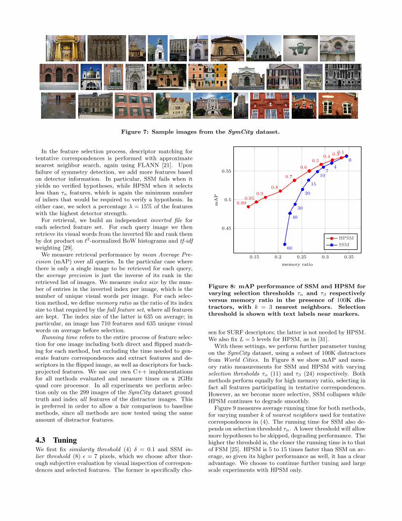
Figure 7: Sample images from the SymCity dataset.

In the feature selection process, descriptor matching fortentative correspondences is performed with approximatenearest neighbor search, again using FLANN [21]. Uponfailure of symmetry detection, we add more features basedon detector information. In particular, SSM fails when ityields no verified hypotheses, while HPSM when it selectsless than τα features, which is again the minimum numberof inliers that would be required to verify a hypothesis. Ineither case, we select a percentage λ = 15% of the featureswith the highest detector strength.

For retrieval, we build an independent inverted file foreach selected feature set. For each query image we thenretrieve its visual words from the inverted file and rank themby dot product on `2-normalized BoW histograms and tf-idfweighting [29].

We measure retrieval performance by mean Average Pre-cision (mAP) over all queries. In the particular case wherethere is only a single image to be retrieved for each query,the average precision is just the inverse of its rank in theretrieved list of images. We measure index size by the num-ber of entries in the inverted index per image, which is thenumber of unique visual words per image. For each selec-tion method, we define memory ratio as the ratio of its indexsize to that required by the full feature set, where all featuresare kept. The index size of the latter is 635 on average; inparticular, an image has 710 features and 635 unique visualwords on average before selection.

Running time refers to the entire process of feature selec-tion for one image including both direct and flipped match-ing for each method, but excluding the time needed to gen-erate feature correspondences and extract features and de-scriptors in the flipped image, as well as descriptors for back-projected features. We use our own C++ implementationsfor all methods evaluated and measure times on a 2GHzquad core processor. In all experiments we perform selec-tion only on the 299 images of the SymCity dataset groundtruth and index all features of the distractor images. Thisis preferred in order to allow a fair comparison to baselinemethods, since all methods are now tested using the sameamount of distractor features.

4.3 TuningWe first fix similarity threshold (4) δ = 0.1 and SSM in-lier threshold (8) ε = 7 pixels, which we choose after thor-ough subjective evaluation by visual inspection of correspon-dences and selected features. The former is specifically cho-

0.15 0.2 0.25 0.3 0.35

0.45

0.5

0.55

0.10.30.40.5

0.6

0.7

0.8

0.90.95

0.99

0

47

10

15

20

30

40

60

memory ratio

mAP

HPSM

SSM

Figure 8: mAP performance of SSM and HPSM forvarying selection thresholds τα and τβ respectivelyversus memory ratio in the presence of 100K dis-tractors, with k = 3 nearest neighbors. Selectionthreshold is shown with text labels near markers.

sen for SURF descriptors; the latter is not needed by HPSM.We also fix L = 5 levels for HPSM, as in [31].

With these settings, we perform further parameter tuningon the SymCity dataset, using a subset of 100K distractorsfrom World Cities. In Figure 8 we show mAP and mem-ory ratio measurements for SSM and HPSM with varyingselection thresholds τα (11) and τβ (24) respectively. Bothmethods perform equally for high memory ratio, selecting infact all features participating in tentative correspondences.However, as we become more selective, SSM collapses whileHPSM continues to degrade smoothly.

Figure 9 measures average running time for both methods,for varying number k of nearest neighbors used for tentativecorrespondences in (4). The running time for SSM also de-pends on selection threshold τα. A lower threshold will allowmore hypotheses to be skipped, degrading performance. Thehigher the threshold is, the closer the running time is to thatof FSM [25]. HPSM is 5 to 15 times faster than SSM on av-erage, so given its higher performance as well, it has a clearadvantage. We choose to continue further tuning and largescale experiments with HPSM only.

1 2 3 4 5

0

100

200

300

k-nearest neighbors

runningtime(m

s)HPSM

SSM, τα = 4

SSM, τα = 10

SSM, τα = 20

Figure 9: Average running time (ms) for HPSM andSSM versus k-nearest neighbors for tentative corre-spondences, where τα is varying for SSM.

k 1 2 3 4 5

τβ = 0.4 0.545 0.566 0.569 0.566 0.568τβ = 0.6 0.522 0.538 0.550 0.551 0.547τβ = 0.8 0.484 0.511 0.515 0.524 0.529

Table 1: HPSM mAP performance versus k-nearestneighbors for varying τβ in the presence of 100K dis-tractors. Chosen parameters and mAP shown inboldface.

Table 1 compares HPSM performance for varying num-ber k of nearest neighbors. Performance almost stabilizes oreven drops with more than 3 neighbors. We therefore choosek = 3 nearest neighbors for our remaining experiments. Wealso choose τβ = 0.4 as default, although there is a furtherexperiment under varying τβ . The average running time ofHPSM for this setting is 16.2ms. Although feature selec-tion is an off-line process, its speed is critical when indexingmillions of images. HPSM is particularly efficient, with arunning time that is negligible compared e.g . to feature de-tection and visual word assignment.

4.4 ComparisonsWorking at larger scale, with up to the full 1M distractor setof World Cities, we compare our selection method to the fullfeature set. We also compare to three alternative, simple se-lection criteria for single images, where in particular a fixednumber of features n is selected, having the highest detectorstrength, largest feature scale σ as in [32], or uniformly atrandom among the full feature set.

Figure 10 shows mAP performance under varying numberof distractor images. While HPSM selection is, not quite un-expectedly, outperformed at small scale, it reaches the fullfeature set performance at large scale. This may be inter-preted as keeping a limited amount of information, whichdegrades quality when matching e.g. a single image pair, butwhich withstands severe distractor noise. An observation ofthe two curve slopes at 106 distractors suggests that HPSM

100 101 102 103

0.4

0.6

0.8

distractors (×103)

mAP

HPSM

Stregth

Scale

Random

Full

Figure 10: Mean average precision comparison ver-sus number of distractors, with τβ = 0.4 for HPSMand a fixed number of features n = 300 for the re-maining selection criteria.

will actually outperform the full feature set at even largerscale.

This experiment is carried out with the default selectionthreshold τβ = 0.4, which yields an average memory ratioof 0.31 on the annotated set, corresponding to 284 selectedfeatures per image on average. To allow a fair comparisonto the alternative selection criteria, we select a fixed numberof n = 300 features per image, so that the average memoryratio is roughly the same. HPSM outperforms all three cri-teria: interestingly, its performance is near that of the threecriteria at small scale, but gradually shifts towards that ofthe full feature set at large scale.

A higher selection threshold τβ would make the processmore selective and decrease memory ratio, at the expense oflower mAP as well. This is a way to trade off index size forretrieval quality. Figure 11 shows this trade-off on the full1M distractor set, revealing that a less selective HPSM caneven outperform the full feature set on mAP for a memoryratio around 35%. On the other hand, its mAP is in generalwell above that of the three alternative criteria for the samememory ratio, with an overhead of 13% on average.

5. DISCUSSIONIt is quite unexpected that symmetry or self-similarity isa generic feature selection criterion that is able to reach orpossibly outperform the full feature set at large scale. On theother hand, it is also unexpected that more local criteria likefeature scale or strength do not in fact give much benefit overrandom selection. Besides this being the first work to applysymmetry for feature selection, we have shown that sym-metry detection is not much different in nature from spatialmatching, so given any advance in one problem it is straight-forward to apply it to the other. In particular, HPSM is thefirst method that is linear in the number of correspondences,being extremely fast in practice.

Among future directions, soft assignment [6] and geome-try verification [31] are probably the first one may combine

0 0.2 0.4 0.6 0.8 1

0.1

0.2

0.3

0.4

memory ratio

mAP

HPSM

Strength

Scale

Random

Full

Figure 11: Mean average precision comparisonagainst memory ratio for varying τβ , n in the pres-ence of 1M distractors.

in the retrieval process. It would be more interesting to ex-tract feature tracks from our single image correspondencesand employ them to find visual synonyms for vocabularylearning, as [20] does from multiple views. All approachesare expected to increase performance without any cost onthe index size.

6. REFERENCES[1] S. Agarwal, N. Snavely, I. Simon, S. M. Seitz, and

R. Szeliski. Building Rome in a day. In ICCV, 2009.

[2] Y. Avrithis, Y. Kalantidis, G. Tolias, and E. Spyrou.Retrieving landmark and non-landmark images fromcommunity photo collections. In ACM Multimedia,2010.

[3] S. Bagon, O. Boiman, and M. Irani. What is a goodimage segment? A unified approach to segmentextraction. In ECCV, 2008.

[4] H. Bay, T. Tuytelaars, and L. Van Gool. SURF:Speeded up robust features. In ECCV, 2006.

[5] O. Boiman, E. Shechtman, and M. Irani. In defense ofnearest-neighbor based image classification. In CVPR,2008.

[6] O. Chum, J. Philbin, J. Sivic, M. Isard, andA. Zisserman. Total recall: Automatic queryexpansion with a generative feature model for objectretrieval. In ICCV, 2007.

[7] H. Cornelius, M. Perdoch, J. Matas, and G. Loy.Efficient symmetry detection using local affine frames.In ECIA, 2007.

[8] P. Doubek, J. Matas, M. Perdoch, and O. Chum.Image matching and retrieval by repetitive patterns.In ICPR, 2010.

[9] S. Gammeter, L. Bossard, T. Quack, and L. V. Gool. Iknow what you did last summer: Object-levelauto-annotation of holiday snaps. In ICCV, 2009.

[10] E. Gavves, C. G. M. Snoek, and A. W. M. Smeulders.Visual synonyms for landmark image retrieval. CVIU,2012.

[11] H. Jegou, M. Douze, and C. Schmid. On theburstiness of visual elements. In CVPR, 2009.

[12] H. Jegou, M. Douze, and C. Schmid. Improvingbag-of-features for large scale image search. IJCV,87(3):316–336, 2010.

[13] H. Jegou, M. Douze, C. Schmid, and P. Perez.Aggregating local descriptors into a compact imagerepresentation. In CVPR, 2010.

[14] Y. Keller and Y. Shkolnisky. An algebraic approach tosymmetry detection. ICPR, pages 186–189, 2004.

[15] J. Knopp, J. Sivic, and T. Pajdla. Avoiding confusingfeatures in place recognition. In ECCV, 2010.

[16] S. Lazebnik, C. Schmid, and J. Ponce. Semi-localaffine parts for object recognition. In BMVC, 2004.

[17] F. Li and J. Kosecka. Probabilistic locationrecognition using reduced feature set. In ICRA, 2006.

[18] D. Lowe. Distinctive image features fromscale-invariant keypoints. IJCV, 60(2):91–110, 2004.

[19] G. Loy and J.-O. Eklundh. Detecting symmetry andsymmetric constellations of features. In ECCV, 2006.

[20] A. Mikulik, M. Perdoch, O. Chum, and J. Matas.Learning a fine vocabulary. In ECCV, 2010.

[21] M. Muja and D. Lowe. Fast approximate nearestneighbors with automatic algorithm configuration. InICCV, 2009.

[22] N. Naikal, A. Yang, and S. Shankar Sastry.Informative feature selection for object recognition viasparse pca. In ICCV, 2011.

[23] M. Perdoch, O. Chum, and J. Matas. Efficientrepresentation of local geometry for large scale objectretrieval. In CVPR, 2009.

[24] F. Perronnin, Y. Liu, J. Sanchez, and H. Poirier.Large-scale image retrieval with compressed Fishervectors. In CVPR, 2010.

[25] J. Philbin, O. Chum, M. Isard, J. Sivic, andA. Zisserman. Object retrieval with large vocabulariesand fast spatial matching. In CVPR, 2007.

[26] G. Schindler, M. Brown, and R. Szeliski. City-scalelocation recognition. In CVPR, 2007.

[27] G. Schindler, P. Krishnamurthy, R. Lublinerman,Y. Liu, and F. Dellaert. Detecting and matchingrepeated patterns for automatic geo-tagging in urbanenvironments. In CVPR, 2008.

[28] E. Shechtman and M. Irani. Matching localself-similarities across images and videos. In CVPR,2007.

[29] J. Sivic and A. Zisserman. Video Google: A textretrieval approach to object matching in videos. InICCV, pages 1470–1477, 2003.

[30] C. Sun and D. Si. Fast reflectional symmetry detectionusing orientation histograms. Real Time Imaging,5(1):63–74, 1999.

[31] G. Tolias and Y. Avrithis. Speeded-up, relaxed spatialmatching. In ICCV, 2011.

[32] P. Turcot and D. Lowe. Better matching with fewerfeatures: the selection of useful features in largedatabase recognition problems. In ICCV, 2009.

[33] T. Tuytelaars, A. Turina, and L. Van Gool.Noncombinatorial detection of regular repetitionsunder perspective skew. PAMI, 2003.