Embed Size (px)
Citation preview

Symbolic Search in Planningand General Game Playing
Peter Kissmann
Dissertation
zur Erlangung des Grades einesDoktors der Ingenieurwissenschaften
– Dr.-Ing. –
Vorgelegt imFachbereich 3 (Mathematik und Informatik)
der Universitat Bremenim Mai 2012

ii
Gutachter: Prof. Dr. Stefan EdelkampUniversitat Bremen
Prof. Dr. Malte HelmertUniversitat Basel
Datum des Kolloquiums: 17. September 2012

Contents
Acknowledgements vii
Zusammenfassung ix
1 Introduction 11.1 Motivation . . . . . . . . . . . . . . . . . . . . . . . . . . . . . . . . . . . . . . . . . . . 11.2 State Space Search . . . . . . . . . . . . . . . . . . . . . . . . . . . . . . . . . . . . . . 31.3 Binary Decision Diagrams and Symbolic Search . . . . . . . . . . . . . . . . . . . . . . . 41.4 Action Planning . . . . . . . . . . . . . . . . . . . . . . . . . . . . . . . . . . . . . . . . 51.5 General Game Playing . . . . . . . . . . . . . . . . . . . . . . . . . . . . . . . . . . . . 61.6 Running Example . . . . . . . . . . . . . . . . . . . . . . . . . . . . . . . . . . . . . . . 8
I Binary Decision Diagrams 9
2 Introduction to Binary Decision Diagrams 112.1 The History of BDDs . . . . . . . . . . . . . . . . . . . . . . . . . . . . . . . . . . . . . 122.2 Efficient Algorithms for BDDs . . . . . . . . . . . . . . . . . . . . . . . . . . . . . . . . 13
2.2.1 Reduce . . . . . . . . . . . . . . . . . . . . . . . . . . . . . . . . . . . . . . . . 132.2.2 Apply . . . . . . . . . . . . . . . . . . . . . . . . . . . . . . . . . . . . . . . . . 142.2.3 Restrict, Compose, and Satisfy . . . . . . . . . . . . . . . . . . . . . . . . . . . . 14
2.3 The Variable Ordering . . . . . . . . . . . . . . . . . . . . . . . . . . . . . . . . . . . . 15
3 Symbolic Search 193.1 Forward Search . . . . . . . . . . . . . . . . . . . . . . . . . . . . . . . . . . . . . . . . 203.2 Backward Search . . . . . . . . . . . . . . . . . . . . . . . . . . . . . . . . . . . . . . . 213.3 Bidirectional Search . . . . . . . . . . . . . . . . . . . . . . . . . . . . . . . . . . . . . . 22
4 Limits and Possibilities of BDDs 234.1 Exponential Lower Bound for Permutation Games . . . . . . . . . . . . . . . . . . . . . . 24
4.1.1 The Sliding Tiles Puzzle . . . . . . . . . . . . . . . . . . . . . . . . . . . . . . . 244.1.2 Blocksworld . . . . . . . . . . . . . . . . . . . . . . . . . . . . . . . . . . . . . 24
4.2 Polynomial Upper Bounds . . . . . . . . . . . . . . . . . . . . . . . . . . . . . . . . . . 274.2.1 Gripper . . . . . . . . . . . . . . . . . . . . . . . . . . . . . . . . . . . . . . . . 274.2.2 Sokoban . . . . . . . . . . . . . . . . . . . . . . . . . . . . . . . . . . . . . . . . 30
4.3 Polynomial and Exponential Bounds for Connect Four . . . . . . . . . . . . . . . . . . . 314.3.1 Polynomial Upper Bound for Representing Reachable States . . . . . . . . . . . . 324.3.2 Exponential Lower Bound for the Termination Criterion . . . . . . . . . . . . . . 354.3.3 Experimental Evaluation . . . . . . . . . . . . . . . . . . . . . . . . . . . . . . . 37
4.4 Conclusions and Future Work . . . . . . . . . . . . . . . . . . . . . . . . . . . . . . . . . 37
iii

iv CONTENTS
II Action Planning 41
5 Introduction to Action Planning 435.1 Planning Tracks . . . . . . . . . . . . . . . . . . . . . . . . . . . . . . . . . . . . . . . . 445.2 The Planning Domain Definition Language PDDL . . . . . . . . . . . . . . . . . . . . . . 44
5.2.1 The History of PDDL . . . . . . . . . . . . . . . . . . . . . . . . . . . . . . . . . 455.2.2 Structure of a PDDL Description . . . . . . . . . . . . . . . . . . . . . . . . . . . 47
6 Classical Planning 536.1 Step-Optimal Classical Planning . . . . . . . . . . . . . . . . . . . . . . . . . . . . . . . 54
6.1.1 Symbolic Breadth-First Search . . . . . . . . . . . . . . . . . . . . . . . . . . . . 546.1.2 Symbolic Bidirectional Breadth-First Search . . . . . . . . . . . . . . . . . . . . 55
6.2 Cost-Optimal Classical Planning . . . . . . . . . . . . . . . . . . . . . . . . . . . . . . . 566.2.1 Running Example with General Action Costs . . . . . . . . . . . . . . . . . . . . 576.2.2 Symbolic Dijkstra Search . . . . . . . . . . . . . . . . . . . . . . . . . . . . . . 586.2.3 Symbolic A* Search . . . . . . . . . . . . . . . . . . . . . . . . . . . . . . . . . 61
6.3 Heuristics for Planning . . . . . . . . . . . . . . . . . . . . . . . . . . . . . . . . . . . . 666.3.1 Pattern Databases . . . . . . . . . . . . . . . . . . . . . . . . . . . . . . . . . . . 676.3.2 Partial Pattern Databases . . . . . . . . . . . . . . . . . . . . . . . . . . . . . . . 73
6.4 Implementation and Improvements . . . . . . . . . . . . . . . . . . . . . . . . . . . . . . 746.4.1 Replacing the Matrix . . . . . . . . . . . . . . . . . . . . . . . . . . . . . . . . . 756.4.2 Reordering the Variables . . . . . . . . . . . . . . . . . . . . . . . . . . . . . . . 766.4.3 Incremental Abstraction Calculation . . . . . . . . . . . . . . . . . . . . . . . . . 786.4.4 Amount of Bidirection . . . . . . . . . . . . . . . . . . . . . . . . . . . . . . . . 78
6.5 International Planning Competitions (IPCs) and Experimental Evaluation . . . . . . . . . 796.5.1 IPC 2008: Participating Planners . . . . . . . . . . . . . . . . . . . . . . . . . . . 806.5.2 IPC 2008: Results . . . . . . . . . . . . . . . . . . . . . . . . . . . . . . . . . . 826.5.3 Evaluation of the Improvements of Gamer . . . . . . . . . . . . . . . . . . . . . . 826.5.4 IPC 2011: Participating Planners . . . . . . . . . . . . . . . . . . . . . . . . . . . 856.5.5 IPC 2011: Results . . . . . . . . . . . . . . . . . . . . . . . . . . . . . . . . . . 87
7 Net-Benefit Planning 917.1 Running Example in Net-Benefit Planning . . . . . . . . . . . . . . . . . . . . . . . . . . 927.2 Related Work in Over-Subscription and Net-Benefit Planning . . . . . . . . . . . . . . . . 947.3 Finding an Optimal Net-Benefit Plan . . . . . . . . . . . . . . . . . . . . . . . . . . . . . 95
7.3.1 Breadth-First Branch-and-Bound . . . . . . . . . . . . . . . . . . . . . . . . . . . 967.3.2 Cost-First Branch-and-Bound . . . . . . . . . . . . . . . . . . . . . . . . . . . . 977.3.3 Net-Benefit Planning Algorithm . . . . . . . . . . . . . . . . . . . . . . . . . . . 98
7.4 Experimental Evaluation . . . . . . . . . . . . . . . . . . . . . . . . . . . . . . . . . . . 1007.4.1 IPC 2008: Participating Planners . . . . . . . . . . . . . . . . . . . . . . . . . . . 1007.4.2 IPC 2008: Results . . . . . . . . . . . . . . . . . . . . . . . . . . . . . . . . . . 1007.4.3 Improvements of Gamer . . . . . . . . . . . . . . . . . . . . . . . . . . . . . . . 101
III General Game Playing 105
8 Introduction to General Game Playing 1078.1 The Game Description Language GDL . . . . . . . . . . . . . . . . . . . . . . . . . . . . 108
8.1.1 The Syntax of GDL . . . . . . . . . . . . . . . . . . . . . . . . . . . . . . . . . . 1098.1.2 Structure of a General Game . . . . . . . . . . . . . . . . . . . . . . . . . . . . . 110
8.2 Differences between GDL and PDDL . . . . . . . . . . . . . . . . . . . . . . . . . . . . 1138.3 Comparison to Action Planning . . . . . . . . . . . . . . . . . . . . . . . . . . . . . . . . 114

CONTENTS v
9 Instantiating General Games 1179.1 The Instantiation Process . . . . . . . . . . . . . . . . . . . . . . . . . . . . . . . . . . . 118
9.1.1 Normalization . . . . . . . . . . . . . . . . . . . . . . . . . . . . . . . . . . . . 1189.1.2 Supersets . . . . . . . . . . . . . . . . . . . . . . . . . . . . . . . . . . . . . . . 1199.1.3 Instantiation . . . . . . . . . . . . . . . . . . . . . . . . . . . . . . . . . . . . . 1239.1.4 Mutex Groups . . . . . . . . . . . . . . . . . . . . . . . . . . . . . . . . . . . . 1249.1.5 Removal of Axioms . . . . . . . . . . . . . . . . . . . . . . . . . . . . . . . . . 1269.1.6 Output . . . . . . . . . . . . . . . . . . . . . . . . . . . . . . . . . . . . . . . . 126
9.2 Experimental Evaluation . . . . . . . . . . . . . . . . . . . . . . . . . . . . . . . . . . . 128
10 Solving General Games 13310.1 Solved Games . . . . . . . . . . . . . . . . . . . . . . . . . . . . . . . . . . . . . . . . . 13410.2 Single-Player Games . . . . . . . . . . . . . . . . . . . . . . . . . . . . . . . . . . . . . 14110.3 Non-Simultaneous Two-Player Games . . . . . . . . . . . . . . . . . . . . . . . . . . . . 143
10.3.1 Two-Player Zero-Sum Games . . . . . . . . . . . . . . . . . . . . . . . . . . . . 14310.3.2 General Non-Simultaneous Two-Player Games . . . . . . . . . . . . . . . . . . . 14410.3.3 Layered Approach to General Non-Simultaneous Two-Player Games . . . . . . . 147
10.4 Experimental Evaluation . . . . . . . . . . . . . . . . . . . . . . . . . . . . . . . . . . . 15010.4.1 Single-Player Games . . . . . . . . . . . . . . . . . . . . . . . . . . . . . . . . . 15010.4.2 Two-Player Games . . . . . . . . . . . . . . . . . . . . . . . . . . . . . . . . . . 153
11 Playing General Games 15711.1 The Algorithm UCT . . . . . . . . . . . . . . . . . . . . . . . . . . . . . . . . . . . . . 158
11.1.1 UCB1 . . . . . . . . . . . . . . . . . . . . . . . . . . . . . . . . . . . . . . . . . 15811.1.2 Monte-Carlo Search . . . . . . . . . . . . . . . . . . . . . . . . . . . . . . . . . 15911.1.3 UCT . . . . . . . . . . . . . . . . . . . . . . . . . . . . . . . . . . . . . . . . . 15911.1.4 UCT Outside General Game Playing . . . . . . . . . . . . . . . . . . . . . . . . . 16011.1.5 Parallelization of UCT . . . . . . . . . . . . . . . . . . . . . . . . . . . . . . . . 163
11.2 Other General Game Players . . . . . . . . . . . . . . . . . . . . . . . . . . . . . . . . . 16511.2.1 Evaluation Function Based Approaches . . . . . . . . . . . . . . . . . . . . . . . 16511.2.2 Simulation Based Approaches . . . . . . . . . . . . . . . . . . . . . . . . . . . . 168
11.3 The Design of the General Game Playing Agent Gamer . . . . . . . . . . . . . . . . . . . 17111.3.1 The GGP Server . . . . . . . . . . . . . . . . . . . . . . . . . . . . . . . . . . . 17111.3.2 The Communicators . . . . . . . . . . . . . . . . . . . . . . . . . . . . . . . . . 17211.3.3 The Instantiators . . . . . . . . . . . . . . . . . . . . . . . . . . . . . . . . . . . 17211.3.4 The Solver . . . . . . . . . . . . . . . . . . . . . . . . . . . . . . . . . . . . . . 17311.3.5 The Players . . . . . . . . . . . . . . . . . . . . . . . . . . . . . . . . . . . . . . 173
11.4 Experimental Evaluation . . . . . . . . . . . . . . . . . . . . . . . . . . . . . . . . . . . 17611.4.1 Evaluation of the Prolog Based Player . . . . . . . . . . . . . . . . . . . . . . . . 17611.4.2 Evaluation of the Instantiated Player . . . . . . . . . . . . . . . . . . . . . . . . . 18111.4.3 Evaluation of the Full Hybrid Player . . . . . . . . . . . . . . . . . . . . . . . . . 18511.4.4 Conclusion . . . . . . . . . . . . . . . . . . . . . . . . . . . . . . . . . . . . . . 190
12 Conclusions and Future Work 19312.1 Contributions . . . . . . . . . . . . . . . . . . . . . . . . . . . . . . . . . . . . . . . . . 19412.2 Future Work . . . . . . . . . . . . . . . . . . . . . . . . . . . . . . . . . . . . . . . . . . 196
Bibliography 199
List of Tables 215
List of Figures 217
List of Algorithms 219

vi CONTENTS
Index 221
A Planning and Game Specifications of the Running Example 225A.1 Classical Planning Unit-Cost Actions . . . . . . . . . . . . . . . . . . . . . . . . . . . . 225
A.1.1 The Domain Description . . . . . . . . . . . . . . . . . . . . . . . . . . . . . . . 225A.1.2 The Problem Description . . . . . . . . . . . . . . . . . . . . . . . . . . . . . . . 226
A.2 Classical Planning With General Action Costs . . . . . . . . . . . . . . . . . . . . . . . . 226A.2.1 The Domain Description . . . . . . . . . . . . . . . . . . . . . . . . . . . . . . . 226A.2.2 The Problem Description . . . . . . . . . . . . . . . . . . . . . . . . . . . . . . . 227
A.3 Net-Benefit Planning . . . . . . . . . . . . . . . . . . . . . . . . . . . . . . . . . . . . . 228A.3.1 The Domain Description . . . . . . . . . . . . . . . . . . . . . . . . . . . . . . . 228A.3.2 The Problem Description . . . . . . . . . . . . . . . . . . . . . . . . . . . . . . . 230
A.4 General Game Playing . . . . . . . . . . . . . . . . . . . . . . . . . . . . . . . . . . . . 232
B BNF of GDDL 235B.1 BNF of GDDL’s Problem File . . . . . . . . . . . . . . . . . . . . . . . . . . . . . . . . 235B.2 BNF of GDDL’s Domain File . . . . . . . . . . . . . . . . . . . . . . . . . . . . . . . . . 235

Acknowledgements
There are many people I would like to say Thankee-sai to.Let me start with my supervisor Stefan Edelkamp. What can I say, it was great working with him. Often,
just talking about some topic suddenly new ways to achieve things become obvious. He is always open tonew ideas and regularly comes up with new ones himself, which often helped when I got stuck somewhere.Also, he is incredibly fast in writing new papers, which of course helped me in getting things published.Judging from the time it took me to finish this thesis it seems that without him it would have taken a lotlonger to get any paper done.
I also wish to extend my thanks to Malte Helmert, who agreed to review this thesis as well. Also,during IPC 2008, when our planner first participated in a competition, he was always very helpful and fastto answer any questions even though he surely was extremely busy, for which I am also very thankful.
Besonderer Dank gebuhrt auch meinen Eltern Klaus und Renate, ohne deren Unterstutzung in allem,das ich anging, vieles erheblich schwieriger geworden ware. Ebenso danke ich meinem Bruder Ralf undseiner Frau Doro, die mich ebenfalls haufig mit hilfreichen Kommentaren unterstutzt haben. Danke furAlles!
Furthermore, I am very grateful to Damian Sulewski and Hartmut Messerschmidt for their helpful com-ments on improving this thesis, and to my former roommate Shahid Jabbar, who pointed out the existenceof the very exciting area of general game playing—without his pointer, this work would be completelydifferent.
Thanks to all the anonymous reviewers who were willing to accept our papers, but also to those whorejected them and offered helpful comments to improve the papers or the research itself, as well as toDeutsche Forschungsgemeinschaft (DFG), who financially supported the projects in which I was employed(ED 74/4 and ED 74/11).
Thanks are also due to my former colleagues at Lehrstuhl 5 at TU Dortmund and my colleagues at AG-KI at the University of Bremen. In Dortmund playing Kicker with the guys (Marco Bakera, Markus Doedt,Stefan Edelkamp, Falk Howar, Martin Karusseit, Sven Jorges, Maik Merten, Stefan Naujokat, JohannesNeubauer, Clemens Renner, Damian Sulewski, Christian Wagner, Thomas Wilk, Holger Willebrandt, andStephan Windmuller), was always a nice distraction from the daily work, though I never became as goodas one might expect with the amount of time we spent on it. Damian, I am sorry that we never were ableto win one of the competitions. In Bremen things seldom got as sweaty, but still the regular board gamenights (with Jan-Ole Berndt, Stefan Edelkamp, Carsten Elfers, Mirko Horstmann, Hartmut Messerschmidt,Christoph Remdt, Martin Stommel, Sabine Veit, and Tobias Warden) at Hartmut’s were always a verywelcome distraction, though in the end I could have done with some fewer sessions of Descent.
I am grateful for all the people who shared a room with me over the past years and never sent me to hell(for my messy desktop or whatever else)—Shahid Jabbar, Damian Sulewski, Till von Wenzlawowicz, MaxGath, and Florian Pantke. Thanks for bringing such a good room climate.
Thanks to Damian for introducing me to geocaching, which made me realize that there is a worldoutside, with fresh air, far away from any computers. . . It is about time that we start another hunt soon.
Furthermore, I wish to thank my good friends back home in Bergkamen (well, at least most of uslived close to Bergkamen once), Alexander and Regina Bartrow, Stefan and Nadine George, Marc-AndreKarpienski and Bernadette Burchard, Christian and Kirsten Trippe, Fabian zur Heiden, Kai Großpietsch,and Holger Blumensaat.
vii

viii ACKNOWLEDGEMENTS
Finally, I wish to thank my companions Veciano Larossa, Gerion, Rondrian Ehrwald, Gerrik Gerriol,Albion Waldpfad, and Grimwulfe—we were ka-tet.
To all those people I somehow forgot I can only Cry your pardon. You know me—I have a brain likea. . . what was I just going to write?

Zusammenfassung
Diese Arbeit behandelt drei Themenkomplexe. Der erste davon, symbolische Suche unter Nutzung vonbinaren Entscheidungsdiagrammen (engl. binary decision diagrams, kurz BDDs) stellt dabei auch direktdas Verknupfungselement mit den anderen beiden Themen, Handlungsplanung und Allgemeines Spiel dar.
Suche ist in vielen Anwendung der kunstlichen Intelligenz (KI) vonnoten. Sei es, dass Graphen durch-sucht, kurzeste Wege ermittelt oder moglichst gute Zuge in einem Spiel gefunden werden sollen (um nurein paar Themengebiete anzuschneiden). In all diesen Fallen ist Suche von hochster Prioritat.
Viele dieser Suchprobleme bringen eine Schwierigkeit mit sich, namlich das sogenannte Suchraumex-plosionsproblem. Dabei handelt es sich um das Problem, dass auch fur vermeintlich kleine Probleme dieMenge an Zustanden, die durchsucht werden muss, exponentielle Ausmaße annehmen kann. Das fuhrt inder Praxis zum einen zu langen Laufzeiten, zum anderen aber auch dazu, dass die Suche nicht vollstandigdurchgefuhrt werden kann, da der zur Verfugung stehende Arbeitsspeicher nicht ausreicht. Aufgrunddes exponentiellen Wachstums der Suchraume besteht auch keine Hoffnung, in absehbarer Zukunft eineRechenleistung und Speicherkapazitat zu erreichen, die mit diesem Problem umgehen kann, da es zumeistnur geringe Verbesserungen von einer Rechnergeneration zur nachsten gibt.
Um das Problem des geringen Speichers zu behandlen kann man auf verschiedene Verfahren zuruck-greifen. Eine Moglichkeit ware die Nutzung externer Algorithmen. Diese fuhren die Suche weitestgehendauf der Festplatte durch, da diese typischerweise uber erheblich mehr Platz verfugt als der interne RAM. Indieser Arbeit beschaftigen wir uns hingegen mit der sogenannten symbolischen Suche.
Bei der symbolischen Suche werden BDDs eingesetzt, um ganze Zustandsmengen zu speichern. Gegen-uber sogenannter expliziter Suche bringen BDDs den Vorteil, dass sie auch große Zustandsmengen sehreffektiv speichern konnen und dabei oftmals erheblich weniger Speicherplatz benotigen als die explizitenVerfahren. Jedoch bringt der Schritt von Einzelzustanden hin zu Zustandsmengen das Problem mit sich,dass wir oftmals vollig neue Algorithmen entwerfen mussen, die fur dieses Konzept ausgelegt sind.
Im Rahmen dieser Arbeit untersuchen wir BDDs auf ihre Komplexitat fur einzelne Suchprobleme. Soist es beispielsweise ein bekanntes Ergebnis, dass BDDs fur Permutationsspiele wie etwa das Schiebepuzzle(15-Puzzle) eine exponentielle Anzahl an internen Knoten benotigen, um alle erreichbaren Zustande abzu-speichern. Wir untersuchen hier einige weitere Probleme und stellen teils untere exponentielle Schranken,teils obere polynomielle Schranken fur die BDD-Großen auf.
Der zweite Teil dieser Arbeit beschaftigt sich mit der Handlungsplanung. In der Handlungsplanungsind eine Menge von Variablen, mit denen sich ein Zustand beschreiben lasst, eine Menge von Aktionen,ein Initialzustand und eine Menge von Zielzustanden gegeben. Basierend auf dieser Eingabe wird nun einsogenannter Plan gesucht, der eine Sequenz von Aktionen darstellt, die, wenn sie in dieser Reihenfolge aufden Initialzustand angewendet werden, letztlich zu einem Zielzustand fuhren. Wir beschaftigen uns hiermit optimalem Planen, das heißt wir suchen nach Planen minimaler Lange.
Haufig werden den einzelnen Aktionen auch unterschiedliche Kosten zugeordnet. In diesem Fall geht esdarum einen Plan zu finden, dessen Kosten (als Summe der Kosten aller Aktionen in diesem Plan) minimalist.
Hier stellen wir symbolische Suchalgorithmen vor, die eben solche Plane finden konnen. Einige setzenauf blinde Suche, wie etwa Breitensuche oder Dijkstras Single-Source Shortest-Paths Algorithmus, andereauf heuristische Suche wie sie in A* eingesetzt wird. Ferner haben wir einen optimalen Handlungsplanerimplementiert, der bereits sehr erfolgreich an internationalen Wettbewerben teilgenommen hat und diesen
ix

x ZUSAMMENFASSUNG
im Jahr 2008 gewann. Im Rahmen der Vorstellung unseres Planers gehen wir weiter auf einige Verbesserun-gen an den zugrundeliegenden Algorithmen ein.
Neben diesen relativ einfach strukturierten Handlungsplanungsproblemen widmen wir uns ferner eineretwas komplexeren Domane, dem sogenannten net-benefit Planen. Darin sind neben den normalen Zielzu-standen weitere Ziele deklariert, die jedoch nicht zwingend erreicht werden mussen, typischerweise jedochin einem hoheren Gewinn resultieren. Entsprechend geht es in dieser Domane nicht mehr nur darum, einenmoglichst kostengunstigen Plan zu finden, sondern einen, der einen moglichst hohen Gewinn (durch dasErfullen der zusatzlichen Ziele) erzielt und dabei moglichst wenig kostet (in Hinblick auf die Summe derAktionskosten).
Fur diese zweite Planungsdomane erarbeiten wir schrittweise einen symbolischen Algorithmus, den wirebenfalls implementiert haben und den resultierenden Planer außerst erfolgreich in einem internationalenWettbewerb eingesetzt haben: Auch dieser konnte den Wettbewerb im Jahre 2008 gewinnen.
Das Spannende an der Handlungsplanung ist die Tatsache, dass wir als Programmierer der Planer nichtwissen, welche Planungsprobleme letztlich tatsachlich zu losen sind. Von einfachen Turmbau- oder Logis-tikproblemen bis zu erheblich komplexeren Bereichen wie einem automatisierten Gewachshaus ist vielesmoglich. Der Planer muss einzig auf Basis der Eingabe intelligente Entscheidungen treffen, um in moglichstkurzer Zeit einen moglichst guten Plan zu finden.
Ein sehr ahnliches Konzept findet sich auch im Allgemeinen Spiel wieder. Hier mussen wir einenSpieler implementieren, der mit einer breiten Auswahl an Spielen konfrontiert werden kann und sie allemoglichst sinnvoll spielen soll. Wie auch in der Handlungsplanung wissen wir als Programmierer vorhernicht, welche Spiele gespielt werden. Entsprechend konnte man das Allgemeine Spiel als eine Erweiterungder Handlungsplanung ansehen. Wahrend in der klassischen Handlungsplanung nur Einpersonenspielemoglich sind, konnen wir im Allgemeinen Spiel mit einer Menge von Gegen- oder Mitspielern konfron-tiert werden. In der Praxis stimmt dieser erste Eindruck jedoch nicht immer vollstandig, unter anderemda es im Allgemeinen Spiel keine Aktionskosten gibt und die Losungslange vollig belanglos ist, solangeman ein moglichst gutes Ziel erreicht. Auf die entsprechenden Gemeinsamkeiten und Unterschiede beiderFormalismen werden wir im Rahmen dieser Arbeit ebenfalls eingehen.
Wahrend viele Forscher im Zusammenhang mit dem Allgemeinen Spiel an moglichst guten Spielerninteressiert sind, liegt unser Hauptaugenmerkt auf dem Losen von Spielen. Im Falle von Einpersonenspielenmochten wir also eine Art von Plan finden, der uns sicher vom Startzustand zu einem moglichst gutenZielzustand fuhrt. Im Falle von Zweipersonenspielen hingegen ist eher eine Strategie gefragt. Diese sagtuns fur jeden erreichbaren Zustand, welchen Zug wir wahlen sollten, um den großtmoglichen Gewinn zuerreichen, auch unter Berucksichtigung der Zuge der Gegner.
In der Vergangenheit wurde schon eine ganze Reihe von Spielen gelost. Dafur wurden jedoch zumeistsehr spezialisierte Verfahren eingesetzt. Einige dieser Verfahren und wie sie zur Losungsfindung genutztwurden werden wir in dieser Arbeit in Erinnerung rufen. Anschließend widmen wir uns einigen Algorith-men, die Allgemeine Spiele losen konnen. Fur diese haben wir erneut auf symbolische Suche gesetzt.
Da viele Spiele einen immens großen Zustandsraum aufweisen, erweist es sich als Vorteil, diese effizientdurch die BDDs verarbeiten zu konnen. Fur BDDs ist es wichtig, eine instanziierte (das heißt variablenfreie)Problembeschreibung zu haben. Im Falle der Handlungsplanung gibt es bereits eine Reihe etablierter In-stanziierer, die die Eingabe in ein solches Format uberfuhren konnen. Im Allgemeinen Spiel gab es solcheInstanziierer bisher noch nicht. Im Rahmen dieser Arbeit wurde ein solcher Instanziierer entwickelt undimplementiert.
Auch wenn unser Hauptaugenmerk ganz klar auf der symbolischen Suche liegt, so haben wir unsdoch auch mit der Programmierung eines Allgemeinen Spielers beschaftigt. Wir werden zunachst einigeetablierte Algorithmen zum Spielen allgemeiner Spiele, etwa Minimax Suche und UCT, vorstellen. An-schließend gehen wir naher auf unseren eigenen Spieler ein. Dieser setzt auf einen hybriden Ansatz, indemwir auf der einen Seite versuchen, das Spiel zu losen, und auf der anderen Seite zwei klassischere Allge-meine Spieler nutzen. Beide Spieler setzen auf UCT, wobei einer eine Schnittstelle zu Prolog nutzt, umdie Eingabe verarbeiten zu konnen, wahrend der andere die Ausgabe unseres Instanziierers verarbeitet unddamit erheblich schneller den Spielbaum durchsuchen kann. Der Vorteil des hybriden Ansatzes gegenubereinem reinen Spieler ist ganz klar, dass wir optimal spielen konnen, wenn eine Losung gefunden wurde unddamit letztlich besser abschneiden konnen als ein normaler Spieler allein.

Chapter 1
Introduction
The man in black fled across the desert, and thegunslinger followed.
Stephen King, The Gunslinger(The Dark Tower Series, Book 1)
1.1 MotivationIn this thesis we are mainly concerned with two sub-disciplines of artificial intelligence, namely actionplanning and general game playing. In both we are confronted with large sets of states (also called statespaces), in which we must search for certain properties. Some examples for these properties are the follow-ing.
• In single-player games or puzzles we want to find a way to establish a goal state, given a state fromwhich we start.
• In multi-player games we want to find a way to reach a goal state where we achieve a reward as highas possible, even if the other players play against us.
• In action planning we want to find a plan transforming an initial state into a goal state, and often wishthe to contain the minimal number of actions or the sum of the costs of the actions within the plan tobe minimal.
• In non-deterministic planning we want to find a policy that specifies for each state an action to take,so that a goal state can be reached independent of any non-determinism.
It is also easy to see some more practical applications of these two sub-disciplines.
• Results from game theory, especially the famous equilibria according to Nash, Jr. (1951), are oftenused in economics and similar disciplines.
• For entertainment we often play games. When playing against a computer we want it act reasonably,because playing against a stupid opponent often is just boring.
• When designing a mobile robot, we want it to be able to reach a certain position, so that it has to finda way to it, given noisy observations of its surroundings.
• In navigation software we want to find a route from a start location to a destination given an entiremap of a country. The desired route can be the shortest, the fastest, the most energy-efficient etc.
1

2 CHAPTER 1. INTRODUCTION
1
2
3
4
5 6
7
8
9
10
11
12 13
14
15
(a) A possible start-ing state.
1 2 3
4 5 6 7
8 9 10 11
12 13 14 15
(b) The desiredgoal state.
Figure 1.1: The 15-PUZZLE.
In all cases we are confronted with state spaces that can be extremely large, a fact that is often referred toas the state space explosion problem. Take the simple n2 − 1-PUZZLE as an example (Figure 1.1 shows aninstance of the well-known 15-PUZZLE). There we have a square board having n2 positions to place tiles,and n2− 1 tiles. Given an initial state described by the positions of the tiles on the board, we want to find away to establish a certain goal state, where all tiles are placed in specified positions. We can move the tilesonly horizontally or vertically onto the one empty position, the blank. At first glance it might appear thatall possible n2! permutations can be reached, but actually Johnson and Story (1879) proved that due to thespecial way the tiles are moved only n2!/2 can really be reached. A typical instance of this puzzle is the 15-PUZZLE, in which we can reach 10,461,394,944,000, i. e., roughly 1× 10¹³ different states. Increasing thewidth and height of the board by only two—resulting in the 35-PUZZLE—the number of reachable statesincreases to 185,996,663,394,950,608,733,999,724,075,417,600,000,000, which is more than 1.8 × 1041.Finding a solution, i. e., a way to move the pieces in order to reach the goal state, requires us to search largeparts of this state space.
Handling such large state spaces requires immense amounts of memory, a resource that is still com-parably scarce and expensive. In the 32 bit era it was only possible to use up to 4GB RAM. Since thechange to 64 bit machines in theory it is possible to use up to 16EB (exa bytes, i. e.,
2106
bytes), which isroughly 16.8 million TB, though in practice in early 2012 personal computers seldom have more than eightor 16GB, and recent mainboards support at most 64GB. On server machines the physical limit is higherand mainboards supporting up to 4TB can be found. Apart from the hardware limits, not all operating sys-tems support so much RAM, e. g.,, the current versions of Microsoft Windows support only up to 192GB(Windows 7), resp. up to 2TB (Windows Server 2008).1 Furthermore, the price for RAM is rather high.Now, early 2012, 8× 8GB RAM can be bought for roundabout 350 Euros.
If the internal memory does not suffice, another way to handle these immense search spaces would beto use external memory algorithms, which make use of hard disks or solid state disks. Nowadays, classicalmagnetic hard disks have a capacity of up to 4TB, while the newer solid state disks, which use flash memoryinstead of magnetic disks and thus have a much better access time, currently have a capacity of up to 3TB.Few desktop mainboards contain up to ten SATA ports to handle the disks, which would allow us to accessup to 40TB in hard disk space. If we compare the prices for RAM with the prices for hard disks (a 4TBmagnetic disk is available for a bit more than 250 Euros; a 3TB solid state disk is available for more than12,500 Euros) we see that using classical RAM is much more expensive than external memory.
Nevertheless, external memory algorithms also bear certain disadvantages. For example, they must bewritten in such a way that the random accesses to the disks are minimized, as the disk operations typicallydominate the entire runtime. In other words, by switching from internal to external memory we can switchfrom the memory problem (too few memory to handle all the states) to a runtime problem (searching thestates on the disk takes a lot longer than in internal memory). Thus, instead of using external memory al-gorithms we use only internal memory but utilize a memory efficient datastructure, namely binary decisiondiagrams (BDDs) Bryant (1986).
In classical explicit search each state is handled on its own, i. e., for each state we must check, if it is agoal state or which actions can be applied in it, resulting in which successor states. Using BDDs and whatis then called symbolic search this is not a good idea, as their operations are typically slower than in explicitsearch and there is no advantage in memory usage in case of single state exploration. Rather, BDDs are
1http://msdn.microsoft.com/en-us/library/windows/desktop/aa366778%28v=vs.85%29.aspx

1.2. STATE SPACE SEARCH 3
made to represent large sets of states, which is where they typically safe huge amounts of memory comparedto explicit search, and there are operators allowing us to generate all the successors of all stored states in asingle step.
In this thesis we handle two domains, namely action planning and general game playing. In both we areconfronted with a similar setting. We have to implement an agent (called a planner or a player, respectively)that is able to find plans in case of action planning or play or solve the games that it is provided in generalgame playing. In contrast to specialized players or solvers we as the programmer do not know what kind ofplanning problem or game the agent will be confronted with, we only know the description languages thatare used to model them. Thus, we cannot insert any domain specific knowledge to improve the agent, butrather it has to come up with efficient ways to search within the state spaces of the specific problems on itsown.
This kind of behavior can be seen as much more intelligent than classical approaches. So far, the bestgame players such as DEEP BLUE (Campbell et al., 2002) for CHESS or CHINOOK (Schaeffer et al., 1992)for AMERICAN CHECKERS were able to dominate the best human players in their respective games, butcannot play any other games, as they simply do not know the rules. Also, they were mainly able to beat thehumans due to good heuristic functions and intelligent search mechanisms. But here, the intelligence doesnot come from the program but rather from the programmer that inserted all the expert knowledge, e. g., therelative importance of the various types of figures in the games, which moves to prefer in general, how toevaluate a certain situation in the game an so on. In an automated action planner or a general game playerthe intelligence inserted is much less prominent, as no such heuristic functions are general enough to coverthe entire set of possibilities. Rather, the agents must come up with such functions themselves and thus actin a much more problem independent manner, which we can perceive as more intelligent behavior.
In the remainder of this introductory chapter we will briefly introduce state space search (Section 1.2),BDDs (Section 1.3), action planning (Section 1.4), and general game playing (Section 1.5), and present asmall example which will be used throughout the thesis (Section 1.6). Furthermore, the following sectionsgive a more detailed overview over the three parts of this thesis. Part I is concerned with BDDs, Part II withaction planning and Part III with general game playing. At the end of this thesis, we draw some conclusionsand point out possibilities for future research in these areas in Chapter 12.
1.2 State Space SearchIn many areas of artificial intelligence we are concerned with state space search (Russell and Norvig, 2010;Edelkamp and Schrodl, 2012). This means that we need to search for certain properties within a set ofstates with transitions between them. Examples for this are finding shortest paths from one state to another,reaching some predefined goal state given a starting state, finding the optimal outcome for each state, ifsome of these states are terminal and an outcome is defined for those. An outcome of a non-terminal statecan be the best (according to some metric) outcome reachable if we are not confronted with some opponentor the outcome that will be reached if all agents act optimally (according to some optimality criterion).
In this work, we are confronted with logic based input, which defines certain binary atoms or fluentsthat specify a state.
Definition 1.1 (Fluent). A fluent is a binary atom that can change over time.
Definition 1.2 (State). Given a set of fluents F a state is the set of all fluents that are currently true. Thus,all fluents not in this set are false.
There are two representations of state spaces, explicit and implicit.
Definition 1.3 (Explicit State Space). An explicit state space corresponds to a given set of states S and aset of transitions T R : S →→ S between these states. Applying the transition relation to a state results in asuccessor of that state. Additionally we typically need an initial state I ∈ S , which determines where thesearch starts, and some terminal states T ⊆ S, which typically do not have any successors.
Such a set of transitions is often given in form of an adjacency list or adjacency matrix. While theformer is linear in the number of transitions (which themselves can be quadratic in the number of states),the latter has a fixed size of |S|2.

4 CHAPTER 1. INTRODUCTION
In this thesis the state spaces are not provided explicitly beforehand, but only implicitly, so that theymust be calculated at runtime.
Definition 1.4 (Implicit State Space). An implicit state space is given by a tuple P = ⟨F ,O, I, T ⟩ with Fbeing the set of fluents constructing states, O a set operators transforming states to successors, I an initialstate, and T a set of terminal states.
Given such an implicit state space declaration we can calculate an explicit one in the following way. Theinitial state I and the terminal states T are already given. Starting at the initial state I we can determinethe set of all reachable states S by repeatedly applying all possible operators to all states found so far untila fix point is reached. Applying operators to a state to determine its successors is also called an expansionof the state. The transitions then correspond to the applied operators and can be stored as well.
In many cases we do not need all reachable states but rather some smaller subset of them. Thus, inthis case we can already safe some memory because we do not have to represent the entire state space inmemory. Also, the set of operators is typically a lot smaller than the full set of transitions, because eachoperator of an implicit state space declaration can affect several states. An example for this might be then2 − 1-PUZZLE, where we have only four operators—i. e., moving the blank up, down, left, or right—,while in an explicit declaration the number of transitions is between two and four times the number ofstates, because in each state two up to four transitions are applicable (two in states where the blank is in acorner, three where it is on the border but not in a corner, four where it is not on the border of the board).
A question that comes to mind is which parts of the state space are necessary, but the answer to thisdepends on the actual problem at hand, so that there is no general answer.
There is a close relation between explicit state spaces and graphs (see, e. g., Edelkamp and Schrodl,2012), so that we can actually transform a state space search problem into a graph search problem and usealgorithms that are designed for that.
Definition 1.5 (Graph). A graph G = (V,E) consists of a set of nodes or vertices V and a set of edges Econnecting certain nodes.
In case of an undirected graph the edges are not oriented, but rather an edge connecting nodes u and vis given by a set u, v.
In case of a directed graph the edges are oriented and thus an edge from node u to node v is given byan ordered pair (u, v). An edge in the opposite direction must not necessarily exist.
A rooted graph is a graph with a special node v0, called the root.
Corollary 1.6 (Equivalence of explicit state spaces and rooted directed graphs). There is a one-to-onemapping between explicit state spaces and rooted directed graphs with a set of distinguished terminalnodes.
Proof Idea. Every node of a graph corresponds to a state in an explicit state space. The root of the graphcorresponds to the initial state, the terminal nodes to the terminal states. An edge (u, v) ∈ E correspondsto a transition from the state represented by node u to the state represented by node v.
In implicit state space search we might say that we generate the graph at runtime and extend it wheneverwe expand some state.
1.3 Binary Decision Diagrams and Symbolic SearchWhile explicit search handles single states, in case of symbolic search (see, e. g., Burch et al., 1992; McMil-lan, 1993) we are confronted with sets of states, which are all expanded in a single step. For this we usebinary decision diagrams (BDDs) (Bryant, 1986), a datastructure used to represent Boolean formulas. Withour definition of states as sets of fluents that are currently true, we can represent a state as a Boolean formulaas well. Each fluent is represented by one binary variable, and a state is the conjunction of all the variablesrepresenting the fluents holding in this state with the negation of those variables representing the fluentsnot holding in it, i. e., each state can be represented by a minterm. A set of states can thus be modeled as a

1.4. ACTION PLANNING 5
disjunction of the minterms representing the states. We will give a more detailed introduction to BDDs inChapter 2.
Set-based search calculates all the successors of a set of states in a single step. This is called an image.Because of this behavior it is easy to perform breadth-first search (BFS) using symbolic search. In caseof BFS we start with the initial state, expand it, continue with the first successor and expand it, continuewith the second successor of the initial state and expand it and so on, until all immediate successors areexpanded. Then we continue with the first successor of the first successor of the initial state and so on. Inother words, we expand the search space in level-order. Using BDDs, we start with the initial state and callthe image. The resulting states are all those of the first BFS level. For the BDD representing that level weagain call the image and receive the second BFS level and so on. Further details on this will be given inChapter 3.
For BDDs as we use them today there are two reduction rules. Due to these rules they can efficientlyrepresent large sets of states without using too much memory; in good cases they can save an exponentialamount of memory compared to an explicit representation. It is hard to predict beforehand whether theBDDs representing certain sets of states are exponentially smaller or not. For some domains it is alreadyknown that they safe exponential amounts of memory (e. g., symmetric functions (see, e. g., Shi et al.,2003)), while for others they are still of exponential size (e. g., for representing the set of all permutationsof a set of variables (Hung, 1997)). We provide the results for some domains from planning and generalgame playing we have analyzed in more detail in Chapter 4, which is based on the following publications.
• Stefan Edelkamp and Peter Kissmann. Limits and Possibilities of BDDs in State Space Search. In23rd AAAI Conference on Artificial Intelligence (AAAI) by Fox and Gomes (eds.). Pages 1452–1453, AAAI Press, 2008.
• Stefan Edelkamp and Peter Kissmann. On the Complexity of BDDs for State Space Search: A CaseStudy in Connect Four. In 25th AAAI Conference on Artificial Intelligence (AAAI) by Burgard andRoth (eds.). Pages 18–23, AAAI Press, 2011.
Especially will we determine a polynomial upper bound for the BDD sizes to represent all reachable statesin GRIPPER, and the problem of CONNECT FOUR is two-fold. On the one hand we can only calculate theset of reachable states, continuing after reaching a terminal state. In that case we will prove that we canfind a variable ordering for which the BDDs remain polynomial. On the other hand we have the terminationcriterion, for which we will prove that even a drastically reduced version of it requires the BDD to haveexponential size.
1.4 Action PlanningOne of the domains we investigate in this thesis is automated action planning. It is interesting because weas a programmer do not know what kind of problem the agent, i. e., the planner, will have to handle, so thatwe must implement a general approach that can work for any problem that can be described.
The description languages used today are quite strong, so that a lot of problems can be described ina concise way. While in the beginning especially simple problems such as the BLOCKSWORLD problem,where several blocks have to be unstacked or stacked to achieve one or more stacks of pre-defined order,have been extensively studied, it is actually possible to model some scenarios closer to real-world problems,such as LOGISTICS problems, where the planner is supposed to find a way to bring some packages from theirstarting locations to their destinations with a number of trucks and airplanes, or some smart greenhouses(the SCANALYZER domain (Helmert and Lasinger, 2010)), where plants are to be moved around conveyors,scanned, and finally returned to their starting positions. Of course, often a lot of abstraction has to bedone in order to come up with a problem that can still be handled by a general approach. A rather generalintroduction to action planning is provided in Chapter 5, where we also introduce the planning domaindefinition language PDDL (McDermott, 1998), which is used to model planning problems.
There are several sub-domains in the general action planning domain, such as classical planning, non-deterministic planning, metric planning, or net-benefit planning. We will also briefly introduce these con-cepts in Chapter 5. In this thesis we are concerned with only two of these sub-domains, namely classicaland net-benefit planning

6 CHAPTER 1. INTRODUCTION
In Chapter 6 we investigate classical planning. There we are given an initial state, some actions tocalculate successor states, a set of goal states, and possibly action costs. The goal for the planner is tofind a plan, i. e., a sequence of actions, that transforms the initial state into one of the goal states, andthat is supposed to be minimal (in the number of actions, or in the sum of the action costs, if we are notonly confronted with unit costs). Our contributions are also proposed in that chapter and are based on thefollowing publications.
• Stefan Edelkamp and Peter Kissmann. Partial Symbolic Pattern Databases for Optimal Sequen-tial Planning. In 31st Annual German Conference on Artificial Intelligence (KI) by Dengel, Berns,Breuel, Bomarius, and Berghofer (eds.). Pages 193–200 of volume 5243 of Lecture Notes in Com-puter Science (LNCS), Springer, 2008.
• Stefan Edelkamp and Peter Kissmann. Optimal Planning with Action Costs and Preferences. In 21stInternational Joint Conference on Artificial Intelligence (IJCAI) by Boutilier (ed.). Pages 1690–1695,2009.
• Peter Kissmann and Stefan Edelkamp. Improving Cost-Optimal Domain-Independent Symbolic Plan-ning. In 25th AAAI Conference on Artificial Intelligence (AAAI) by Burgard and Roth (eds.). Pages992–997, AAAI Press, 2011.
The main contributions are partial pattern databases in the symbolic setting, while they before were onlydefined for explicit search, and the implementation of a classical planner. For the planner we also proposea number of improvements that greatly enhance its power to find more solutions.
In Chapter 7 we are concerned with net-benefit planning. In this sub-domain we are given an initialstate, actions to calculate successor states, a set of goal states one of which must be reached by a plan andan additional set of preferences, which correspond to properties of the goal states that are to be preferred.The actions can have certain costs, while satisfying properties gives us certain rewards. The goal of aplanner is to find a plan that reaches a goal and achieves the maximal net-benefit, which is the total rewardfor satisfying the desired properties minus the total cost of the actions needed to satisfy them. The approachwe propose in that chapter is based on the following publication.
• Stefan Edelkamp and Peter Kissmann. Optimal Planning with Action Costs and Preferences. In 21stInternational Joint Conference on Artificial Intelligence (IJCAI) by Boutilier (ed.). Pages 1690–1695,2009.
The algorithm is based on a symbolic variant of branch-and-bound search and allows us to find optimalplans in this setting. We have implemented this algorithm and included it into a full-fledged net-benefitplanner.
1.5 General Game PlayingGeneral game playing (GGP) goes in a similar direction as automated action planning, but it can be seento be even more general. In general game playing the agent, i. e., the player, has to handle any game thatcan be described by the used description language without intervention of a human, and also without theprogrammer knowing what game will be played. Instead it has to come up with a good strategy on its own.
Nowadays the most used description mechanism is the game description language GDL (Love et al.,2006). In its original form it allows the description of simultaneous-move multi-player games2 that arediscrete, deterministic, finite, and where all players have full information of the current state. A morerecent extension, GDL-II (for GDL for games with incomplete information) (Thielscher, 2010) lifts the twomost constricting conditions, i. e., it allows to model games that can have some element of chance, as it ispresent in most dice games, and also provides a concept to conceal parts of the states from the players inorder to model incomplete information games, as it is needed for most card games.
In this work we are only concerned with the concept of deterministic games with full information for allplayers, as even in this domain research still seems to be quite at the beginning. We will start by describing
2Multi-player here means games for one or more players.

1.5. GENERAL GAME PLAYING 7
the idea of general game playing in more detail in Chapter 8. There we will also introduce all the elementsof GDL.
One problem of GDL, similar to PDDL, is that it comes with a lot of variables, while for BDDs weare dependent on grounded input. In the beginning we modeled the games in a slightly extended PDDLderivative by translating the GDL input by hand. We did this in order to use existing grounders from theplanning domain, as so far there were none present in general game playing. Later we decided to implementour own grounding utility, or instantiator, so that we can use our symbolic algorithms in a fully automatedgeneral game player as well. Two approaches we implemented to instantiate general games are describedin Chapter 9, which is based on the following publications.
• Peter Kissmann and Stefan Edelkamp. Instantiating General Games. In 1st IJCAI-Workshop onGeneral Intelligence in Game-Playing Agents (GIGA). Pages 43–50, 2009.
• Peter Kissmann and Stefan Edelkamp. Instantiating General Games using Prolog or DependencyGraphs. In 33rd Annual German Conference on Artificial Intelligence (KI) by Dillmann, Beyerer,Schultz, and Hanebeck (eds.). Pages 255–262 in volume 6359 of Lecture Notes in Computer Science(LNCS), Springer, 2010.
For several games optimal solutions are already known. In this context we distinguish three differenttypes of solutions (Allis, 1994), from ultra-weak, where we only know whether the starting player wins thegame but no actual strategy is known, over weak, where we know what move to choose in any state that canbe reached, no matter what the opponent does, up to strong, where we know the optimal move to take forevery reachable state, i. e., even for states that are only reachable if we chose a sub-optimal move ourselves.
We implemented a symbolic solver that can find strong solutions for single-player games as well asnon-simultaneous two-player games. After a discussion of specialized approaches that yield solutions forsome games we will present our general symbolic approach in Chapter 10, which is based on the followingpublications.
• Stefan Edelkamp and Peter Kissmann. Symbolic Explorations for General Game Playing in PDDL.In 1st ICAPS-Workshop on Planning in Games. 2007.
• Stefan Edelkamp and Peter Kissmann. Symbolic Classification of General Two-Player Games. In31st Annual German Conference on Artificial Intelligence (KI) by Dengel, Berns, Breuesl, Bomarius,and Berghofer (eds.). Pages 185–192 of volume 5243 of Lecture Notes in Computer Science (LNCS),Springer, 2008.
• Peter Kissmann and Stefan Edelkamp. Layer-Abstraction for Symbolically Solving General Two-Player Games. In 3rd International Symposium on Combinatorial Search (SoCS). Pages 63–70,2010.
Normally the overall goal in general game playing is to implement a player that can play general games,and play them as good as possible. In practice it must decide which move to take in a very short time. Sym-bolic search with BDDs is often quite time-consuming, so that it is not too well suited for this task. Insteadwe decided to implement a hybrid player. One part is a rather traditional player that is based on explicitsearch using a simulation-based approach called upper confidence bounds applied to trees (UCT) (Kocsisand Szepesvari, 2006), which has been the most successful in recent years. We actually implemented twoof these players, one making use of Prolog in order to handle the original input, and another one capable tohandle the grounded input we generate for the BDD based solver, which is a lot faster than the Prolog basedplayer. The other part of the hybrid player is our BDD based solver, so that games that are solved can beplayed optimally. Our main interest lies with symbolic search, which means that the explicit search play-ers are not yet high-performance, even though they can play reasonably well in several games. The UCTapproach along with several extensions and ways for parallelizing it as well as our player are presented inChapter 11, which is based on the following publications.
• Stefan Edelkamp, Peter Kissmann, Damian Sulewski, and Hartmut Messerschmidt. Finding the Nee-dle in the Haystack with Heuristically Guided Swarm Tree Search. In Multikonferenz Wirtschaftsin-formatik – 24th Workshop on Planung / Scheduling und Konfigurieren / Entwerfen (PuK) by Schu-mann, Kolbe, Breitner and Frerichs (eds.). Pages 2295–2308, Universitatsverlag Gottingen, 2010.

8 CHAPTER 1. INTRODUCTION
p1
p2
p3 p6
p8
p9
p7
p5
p4
p0
Figure 1.2: The running example.
• Peter Kissmann and Stefan Edelkamp. Gamer, a General Game Playing Agent. In volume 25 ofKI—Zeitschrift Kunstliche Intelligenz (Special Issue on General Game Playing). Pages 49–52, 2011.
1.6 Running ExampleThroughout this work we will use a simple example to explain things. This example is slightly inspired bythe opening words of Stephen King’s The Dark Tower series, i. e., “The man in black fled across the desert,and the gunslinger followed”. We model the desert as a graph consisting of ten locations p0 to p9, whichare connected by undirected edges, so that the protagonists can move from one location to a connected one(cf. Figure 1.2). Location p0 serves as the entrance to the desert, while it can be left only from location p9.
We take this graph as the basis whenever we refer to our running example, though it will be refined inseveral places. For example, we must specify locations for the man in black and the gunslinger to start. Also,we must specify what the goal of the planner respectively the players might be. If we allow actions to havedifferent costs we can assume that some paths are harder to travel on than others, maybe due to less shadeor more and steeper dunes, which we can model by using different weights for the edges. Additionally wemight assume that it is necessary to find some water to drink in order not to die of dehydration. Furthermoreit might be that the two protagonists move with different speeds. Further details will be given when theyare needed in the corresponding places in the remainder of this thesis.

Part I
Binary Decision Diagrams
9


Chapter 2
Introduction to Binary DecisionDiagrams
Logic is the beginning, not the end, of Wisdom.
Captain Spock in Star Trek VI(The Undiscovered Country)
Binary decision diagrams (BDDs) are a memory-efficient data structure used to represent Boolean func-tions as well as to perform set-based search.
Definition 2.1 (Binary Decision Diagram). A binary decision diagram (BDD) is a directed acyclic graphwith one root node and two terminal nodes, i. e., nodes with no outgoing edges, the 0 sink and the 1 sink.Each non-terminal node corresponds to a binary variable, so that it has two outgoing edges, the low edgefor the variable being false (or 0) and the high edge for it being true (or 1).
Definition 2.2 (Satisfying Assignment). A path in a BDD starting at the root and ending in the 1 sinkcorresponds to a satisfying assignment of the variables. The variables touched by the path are assigned thevalue according to the outgoing edge, all others can take any value.
Given a BDD, it is fairly easy to check whether an assignment of the variables is satisfying or not.Starting at the root, it is only necessary to follow the outgoing edge corresponding to the value of thevariable in the assignment. If finally the 1 sink is reached, the assignment is satisfying; if the 0 sink isreached it is not.
BDDs are often used to store sets of states. According to our definition of a state (cf. Definition 1.2)a state is specified by those binary fluents (or variables, as we typically call them in the context of BDDs)that are true in that state, while all other variables must be false. Thus, a state can be seen as a simpleconjunction. Let V be the set of all variables and let V1 ⊆ V and V0 ⊆ V be the set of variables being trueor false, respectively, with V1 ∩ V0 = ∅ and V1 ∪ V0 = V . Then a state s can be described by the Booleanfunction
bf (s) =
v1∈V1
v1 ∧
v0∈V0
¬v0.
A set of states S can then be described the disjunction of all the Boolean functions describing the stateswithin the set:
bf (S) =s∈S
bf (s) .
This being a Boolean function it is of course possible to represent the set of states by a BDD. Any satisfyingassignment then corresponds to a state that is part of the set represented by the BDD.
The BDD representing the empty set consists of only the 0 sink and is denoted by ⊥, while the onethat consists only of the 1 sink and is denoted by ⊤ represents the set of all states describable by the set ofvariables, i. e., for n binary variables it corresponds to all possible 2n states.
11

12 CHAPTER 2. INTRODUCTION TO BINARY DECISION DIAGRAMS
In the following sections of this chapter we will give a brief overview of the history of BDDs, followedby a short introduction to the most important efficient algorithms to handle and create BDDs and somenotes on the importance of the variable ordering that was introduced to reduce the BDDs’ sizes.
Chapter 3 introduces the use of BDDs in state space search, which is then called Symbolic Search.Finally, in Chapter 4 we present theoretical results on BDD sizes in some planning and game playingdomains.
2.1 The History of BDDsBDDs go back more than 50 years, when Lee (1959) proposed the use of, what he then called, binary-decision programs. They already consisted of some of the basic elements, i. e., a set of binary variablesalong with the 0 and 1 sink to model Boolean functions.
Akers (1978) came up with the name we still use today and already presented some approaches toautomatically generate BDDs to represent Boolean functions using Shannon expansions (Shannon, 1938)or truth tables. Nevertheless, he did not limit the generation of the BDDs in any way, so that variables mightappear more than once on certain paths from the root node to one of the sinks. Apart from the name and thesimilarity in the graphical representation he already saw the possibility to reduce the BDDs in some casesbut did not provide an algorithmic description of this process.
Finally, Bryant (1986) proposed the use of a predefined ordering of the binary variables.
Definition 2.3 (Variable Ordering). Given a set of binary variables V , the variable ordering π is a permu-tation of the variables π : V →→ 0, . . . , |V| − 1.
Due to this ordering a BDD can be organized in layers, each of which contains nodes representing thesame variable. These layers can be addressed by a unique index, which is the position of the correspondingvariable within the ordering. Thus, the root node resides in the layer with smallest index 0. All edgesare directed from nodes of one layer to those of other layers with greater index, so that any path startingat the root visits the variables in the same predefined order. With the fixed ordering it is thus possible toautomatize the process of generating a BDD given any Boolean function. Such a BDD is also called anOrdered Binary Decision Diagram (OBDD).
Definition 2.4 (Ordered Binary Decision Diagram). An ordered binary decision diagram (OBDD) is a BDDwhere the variables represented by the nodes on any path from the root to one of the sinks obey the samefixed variable ordering.
Due to the fixed variable ordering an OBDD can be reduced by following two simple rules, which aredepicted in Figure 2.1.
Definition 2.5 (Reduction Rules). For OBDDs two reduction rules are known.
1. If the two successors of a node u reached when following the low and the high edge actually are thesame node v then u can be removed from the BDD and all ingoing edges are redirected to v. This isdepicted in Figure 2.1a.
2. If two nodes u1 and u2 represent the same variable and the node reached by the low edge of u1 isthe same as the one reached by the low edge of u2 and the node reached by the high edge of u1 is thesame as the one reached by the high edge of u2 then u1 and u2 can be merged by removing u2 andredirecting all ingoing edges to u1. This is depicted in Figure 2.1b.
The resulting OBDD is also called a Reduced Ordered Binary Decision Diagram (ROBDD).
Definition 2.6 (Reduced Ordered Binary Decision Diagram). A reduced ordered binary decision diagram(ROBDD) is an OBDD where the reduction rules are repeatedly applied until none of them can be appliedany more.

2.2. EFFICIENT ALGORITHMS FOR BDDS 13
vj vj
vi
(a) Rule 1. Removal of nodes withequal successors.
vj
vi
vk
vj
vi
vk
vi
(b) Rule 2. Merging of nodes withsame low and high successors.
Figure 2.1: The two rules for minimizing BDDs for a given variable ordering π = v1, . . . , vn (i < j andi < k). Solid lines represent high edges, dashed ones low edges.
0 1
x1
x2
(a) Conjunction (v1 ∧ v2).
0 1
x1
x2
(b) Disjunction (v1 ∨ v2).
0 1
x1
(c) Negation (¬v1).
0 1
x1
x2 x2
(d) Equivalence (v1 ↔ v2).
Figure 2.2: BDDs representing basic Boolean functions. Solid lines represent high edges, dashed ones lowedges.
An ROBDD is a canonical representation of the given Boolean function, i. e., two equivalent formulasare represented by the same ROBDD (apart from isomorphisms). Due to the reduction several of theinternal nodes can be saved, so that ROBDDs are quite memory-efficient. Throughout this work we areonly concerned with ROBDDs, so that whenever we write about BDDs we actually refer to ROBDDs.
For the set of variables V = v1, v2 and the ordering (v1, v2) a number of simple ROBDDs represent-ing some basic Boolean functions are depicted in Figure 2.2.
Another extension Bryant (1986) proposed is to use one BDD with several root nodes to represent anumber of different Boolean functions instead of a single BDD for each one. This brings the advantage ofsharing the same nodes, i. e., for representing formulas whose BDD representation is largely the same wedo not need to store the same BDD nodes more than once in main memory, so that these are even morememory-efficient. Such BDDs are called Shared BDDs (Minato et al., 1990).
2.2 Efficient Algorithms for BDDsAlong with the idea of using a fixed variable ordering resulting in OBDDs, Bryant (1986) also proposedseveral algorithms to automatically generate BDDs and to work with them efficiently.
2.2.1 ReduceOne of the most important algorithms is the Reduce algorithm, which is an implementation of the reductionrules to create ROBDDs.
Bryant (1986) proposed a version that has a time complexity of O (|V | log |V |) with |V | being thenumber of nodes within the original BDD. It starts at the two sinks and works in a layer-wise mannerbackwards towards the root. In each layer it checks the applicability of the two rules and deletes those

14 CHAPTER 2. INTRODUCTION TO BINARY DECISION DIAGRAMS
nodes for which one can be applied. Once the root node is reached the BDD is fully reduced and thus ofminimal size.
Later, Sieling and Wegener (1993) have shown that using two phases of bucket sort the time complexityis reduced to linear time O (|V |).
2.2.2 ApplyAnother important algorithm is the Apply algorithm. In contrast to other approaches, there is no need fordifferent algorithms for each Boolean operator. Instead, Apply generates a new BDD given two existingones and the operator for the specified composition. The idea is as follows. The algorithm starts at the rootnodes of each BDD. For the current nodes it adds a new node into the resulting BDD. If the current nodes ofboth BDDs are in the same layer, both low successors as well as both high successors are combined usingthe Apply algorithm. Otherwise it combines the low and high successor of the node from the layer withsmaller index with the other node. The values of the sinks are determined according to the rules for thespecified Boolean operator. Finally, the Reduce algorithm is called to make sure that the resulting BDD isreduced as well.
This algorithm would require time exponential in the number of variables, so Bryant (1986) also pro-posed two extensions. The first one makes use of a table to store the result of applying two nodes. This way,the same operation does not have to be performed more than once. The second one improves the algorithmby adding a sink already when one of the two current nodes is a sink with a controlling value (e. g., 1 forthe disjunction or 0 for the conjunction). With these extensions the algorithm generates the combination oftwo BDDs with |V1| and |V2| BDD nodes in time O (|V1| |V2| log (|V1|+ |V2|)).
2.2.3 Restrict, Compose, and SatisfyFurther algorithms Bryant (1986) proposed are Restrict, Compose, Satisfy-one, Satisfy-all, and Satisfy-count. In Restrict, a variable of the represented formula is assigned a fixed Boolean value and the resultingBDD is returned. This algorithm can be performed in time O (|V | log |V |), with |V | being the number ofnodes in the original BDD. In Compose, a variable is replaced not just by a constant but by a full Booleanfunction. This can be done in time O
|V1|2 |V2| log (|V1|+ |V2|)
for two BDDs of sizes |V1| and |V2|.
While all of the other algorithms create or reorganize the BDDs, the Satisfy algorithms are concernedwith the sets of satisfying assignments. The Satisfy-one algorithm returns exactly one of the satisfyingassignments. Given an initial array of Boolean values, it starts at the root of the BDD and operates towardsthe sinks. For each encountered node it checks if the successor according to the provided Boolean value isthe 0 sink. In that case it flips the value in the array and continues with the other successor. Otherwise itdoes not change the value in the array and continues with the indicated successor. As soon as the 1 sink isreached the array holds a satisfying assignment. Thus, at mostO (n) nodes must be evaluated, with n beingthe number of variables.
Satisfy-all returns the set of all satisfying assignments. Here, the idea is to start at the root node andto follow all possible paths toward the 1 sink. If a node for the current index is present on the currentpath, both successors are investigated next. If for some index i no such node is present, i. e., the formula isindependent of vi for the current assignment, both cases (vi = 1 and vi = 0) are investigated and returnedin the end. Thus, the algorithm can be performed in time O (n |Sf |) with n being the number of variablesand |Sf | the number of satisfying assignments for the represented Boolean function f .
The Satisfy-count returns the number of satisfying assignments. For this, the algorithm assigns a valueαv to each node v. For the terminal nodes, the value is the corresponding value (0 / 1). For a non-terminalnode v, the value is set to
αv = αlow(v)2index(low(v))−index(v)−1 + αhigh(v)2
index(high(v))−index(v)−1
with low (v) and high (v) being the successor of v along the low and high edge, respectively, and index (v)the ordering’s index of the variable that the node v represents. This way, the complete BDD is traversedonly once in a depth-first manner and the resulting runtime is at mostO (|V |) with |V | being the number ofnodes in the BDD.

2.3. THE VARIABLE ORDERING 15
0 1
x1
y1
x2
y2
x3
y3
(a) Good variable ordering.
0 1
x1
x2 x2
x3 x3 x3 x3
y1y1y1y1
y2 y2
y3
(b) Bad variable ordering.
Figure 2.3: Two possible BDDs representing DQF3. Solid lines represent high edges, dashed ones lowedges.
2.3 The Variable OrderingFor many Boolean functions the corresponding BDD can be of polynomial or even linear size, given a goodvariable ordering π, although the number of satisfying assignments (i. e., the number of states) might beexponential in the number of variables. One such case is the disjoint quadratic form (DQF).
Definition 2.7 (Disjoint Quadratic Form). For two sets of binary variables x1, . . . xn and y1, . . . , yn thedisjoint quadratic form DQFn is defined as
DQFn (x1, . . . , xn, y1, . . . , yn) := (x1 ∧ y1) ∨ (x2 ∧ y2) ∨ · · · ∨ (xn ∧ yn) .
On the one hand, if the two sets of variables are ordered in an interleaved fashion the correspondingBDD is of linear size.
Proposition 2.8 (Linear size of a BDD for DQF). Given the variable ordering π = (x1, y1, . . . , xn, yn),the BDD representing the DQFn contains 2 (n+ 1) nodes.
On the other hand, for the DQF we can also find a bad variable ordering, so that the size of the corre-sponding BDD is exponential in n.
Proposition 2.9 (Exponential size of a BDD for DQF). The BDD representing the DQFn contains 2n+1
nodes if the variable ordering π = (x1, . . . , xn, y1, . . . , yn) is chosen.
Figure 2.3 illustrates both cases for the DQF3.There are also some functions for which any BDD contains an exponential number of nodes, no matter
what variable ordering is chosen. One example the integer multiplication. Given two inputs a1, . . . , an andb1, . . . , bn, the binary encoding of two integers a and b with a1 and b1 being the least significant bits. Thenthere are 2n outputs, which correspond to the binary encoding of the product of a and b. These can bedescribed by functions mul i (a1, . . . , an, b1, . . . , bn) (1 ≤ i ≤ 2n). For a permutation π of 1, . . . , 2n, letG (i, π) be a graph, which represents the function mul i
xπ(1), . . . , xπ(2n)
for inputs x1, . . . , x2n. Then
the following Theorem can be proved (Bryant, 1986).

16 CHAPTER 2. INTRODUCTION TO BINARY DECISION DIAGRAMS
0 1
x′1
x′2 x′2
x′3
x′4
x′5
x′6
x′3 x′3
x′4 x′4 x′4
x′5 x′5 x′5 x′5
x′6 x′6 x′6 x′6 x′6
2 3 4 5 6
(a) Not fully reduced BDD. The sinks represent the numbers ofhigh edges on the path from the root. In a real BDD the sinkswould be replaced by the 0 or 1 sink, dependent on the actualfunction.
0 1
x′2
x′3
x′4
x′5
x′6x′6
x′5
x′4
x′3
x′2
x′1
(b) Reduced BDD for the casethat the function represents allcases with an odd number of 1sin the input.
Figure 2.4: BDDs for a symmetric function with six arguments (f (x1, . . . , x6)), with (x′1, . . . , x′6) being
an arbitrary permutation of (x1, . . . , x6). Solid lines represent high edges, dashed ones low edges.
Theorem 2.10 (Exponential size of any BDD for integer multiplication). For any variable ordering π thereexists an i, 1 ≤ i ≤ 2n, so that G (i, π) contains at least 2n/8 nodes.
Finally, for some functions any variable ordering results in a polynomial sized BDD. Symmetric func-tions are an example for this behavior.
Definition 2.11 (Symmetric Function). A function f : 0, 1n →→ 0, 1 is called symmetric if the valueremains the same, independent of the order of the arguments, i. e., if f (x1, . . . , xi, . . . , xj , . . . , xn) =f (x1, . . . , xj , . . . , xi, . . . , xn) for all i, j ∈ 1, . . . , n.
Thus, for a symmetric function the truth value depends only on the number of 1s in the input. Any BDDrepresenting a symmetric function is of size O
n2, no matter what variable ordering is used (see, e. g.,
Shi, Fey, and Drechsler, 2003).
Theorem 2.12 (Quadratic size of any BDD for symmetric functions). For any symmetric function f :0, 1n →→ 0, 1 a BDD contains at most O
n2
nodes, no matter what variable ordering is used.
Proof. As the value of a symmetric function does not depend on the order of the input variables it is clearthat any BDD, no matter what ordering is used, is of the same size. It is possible to generate a (not fullyreduced) BDD as shown in Figure 2.4a for any such function, which contains O
n2
BDD nodes and isthus quadratic in the number of variables. All nodes on a diagonal going from top-right to bottom-left canbe reached by the same number of high edges. Due to the fact that swapping two variables does not matter,the low successor of the high successor of some node always equals the high successor of the low successorof the same node. Thus, the BDD contains exactly n (n+ 1) /2 + 2 nodes. Reducing such a BDD cannotincrease the size, so that a reduced BDD cannot contain more than O
n2
nodes as well (cf. Figure 2.4bfor an example).
For many functions there are good variable orderings and finding these is often crucial, as due to theApply algorithm operations such as the conjunction or disjunction of two BDDs take time in the order

2.3. THE VARIABLE ORDERING 17
of the size of the two BDDs. Yet, finding an ordering that minimizes the number of BDD nodes is Co-NP-complete (Bryant, 1986). Furthermore, the decision whether a variable ordering can be found so thatthe resulting BDD contains at most s nodes, with s being specified beforehand, is NP-complete (Bolligand Wegener, 1996). Finally, Sieling (2002) proved that there is no polynomial time algorithm that cancalculate a variable ordering so that the resulting BDD contains at most c times as many nodes as the onewith optimal variable ordering for any constant c > 1, so that we cannot expect to find a good variableordering using reasonable resources. This shows that using heuristics to calculate a variable ordering (see,e. g., Fujita et al., 1988; Malik et al., 1988; Butler et al., 1991) is a sensible approach.

18 CHAPTER 2. INTRODUCTION TO BINARY DECISION DIAGRAMS

Chapter 3
Symbolic Search
Where do I go?
Never had a very real dream before.Now I got a vision of an open door.Guiding me home, where I belong,Dreamland I have come.
Oh where do I go?
Avantasia, The Towerfrom the Album The Metal Opera
State space search is an important topic in many areas of artificial intelligence (Russell and Norvig,2010; Edelkamp and Schrodl, 2012). No matter if we want to find a shortest path from one location toanother, or some plan transforming a given initial state to another state satisfying a goal condition, or astrategy specifying good moves for a game, in all these (and many more) cases search is of high importance.
In explicit state search we need to come up with good data structures to represent the states efficientlyor algorithms for fast transformation of states. In case of symbolic search (see, e. g., Burch et al., 1992;McMillan, 1993) with BDDs the data structure to use is already given. As to efficient algorithms, here weneed to handle things in a different manner compared to explicit search. While explicit search is concernedwith expansion of single states and the calculation of one successor after the other, in symbolic search weneed to handle sets of states.
To perform symbolic search we need two sets of binary variables, both ranging over the entire set ofvariables needed to represent a state. One set, V , is needed to store the current states, while the other set, V ′,stores the successor states. Because the variables true in a successor state are often closely related to thosetrue in the current state we decided to store the two sets in an interleaved fashion (Burch et al., 1994). Withthese sets we can represent a transition relation, which connects the current states with their successors.
As we have mentioned in the introduction, in this work we are only concerned with implicit searchspaces, i. e., given an initial state, we can calculate all successor states by applying all possible operators.This we can repeat for the successors, until in the end all states are calculated and the full state space residesin memory. Actually, in practice we are often also given some terminal states and try to reduce the statespace to be stored as much as possible, e. g., by using some heuristic to determine whether a successoractually brings us closer to a terminal state. Nevertheless, in the following we will present the most basicalgorithms, i. e., pure symbolic breadth-first search (BFS) and its bidirectional extension.
For a given set of operators O, an operator o ∈ O consists of a precondition preo and some effects eff o
to specify the changes to a state satisfying the precondition, which enables us to calculate the successorstate.
19

20 CHAPTER 3. SYMBOLIC SEARCH
Definition 3.1 (Transition Relation). Given an operator o = (preo, eff o) ∈ O the transition relation T Ro
is defined as
T Ro (V,V ′) := preo (V) ∧ eff o (V ′) ∧ frameo (V,V ′)
with frameo being the frame for operator o, which specifies what part of the current state does not changewhen applying o.
Combining these transition relations results in a single (monolithic) transition relation T R by calculat-ing the disjunction of the transition relations T Ro of all operators o ∈ O.
Definition 3.2 (Monolithic Transition Relation). Given a set of operatorsO and a transition relation T Ro
for each o ∈ O, the monolithic transition relation T R is defined as
T R (V,V ′) :=o∈OT Ro (V,V ′) .
3.1 Forward Search
To calculate the successors of a set of states, the image operator (see, e. g., Burch et al., 1992) is used.
Definition 3.3 (Image Operator). Given a set of states current , specified in V , all successor states arecalculated by the image operator
image (current) := (∃V . T R (V,V ′) ∧ current (V)) [V ′ → V] .
In this formula [V ′ → V] denotes the replacement of all variables of V ′ by those of V , so that thesuccessor states are represented in V and we can continue the search.
This combination of conjunction and existential quantification is also called the relational product.Though we are able to find efficient variable orderings for many problems we cannot expect to be able tocalculate exponential search spaces in polynomial time. This comes from the fact that the calculation of therelational product is in itself NP-complete, which was proved by McMillan (1993) by reduction from the3-SAT problem.
Note that it is not essential to use a monolithic transition relation. For many problems the BDD for themonolithic transition relation is larger than the sum of the sizes of the transition relations for the operators.Thus, the image calculations take even longer. Also, the creation of the monolithic transition relation takesa long time and it consumes a large amount of memory. Instead, we can manage the transition relations ofall operators separately, apply the relational product to one after the other and calculate the disjunction ofthese smaller sets of successor states afterward (Burch et al., 1991).
Definition 3.4 (Single-Operator Image Operator). Given a set of states current , specified in V , the succes-sor states resulting from the application of the operator o ∈ O is calculated by the single-operator imageoperator
imageo (current) := (∃V . T Ro (V,V ′) ∧ current (V)) [V ′ → V] .
Corollary 3.5 (Image operator with non-monolithic transition relation). The image operator can be rewrit-ten to use the smaller transition relations T Ro for each operator o ∈ O.

3.2. BACKWARD SEARCH 21
Algorithm 3.1: Symbolic Breadth-First SearchInput: Implicit definition of a state space problem P = ⟨V,O, I⟩.Output: BDD reach representing the set of all states reachable from I.
1 reach ← I // Start at initial state I.2 newStates ← reach // newStates is used for stopping once all states have been generated.3 while newStates = ⊥ do // Repeat until no new states found in last iteration.4 newStates ← image (reach) ∧ ¬reach // Calculate new successor states.5 reach ← reach ∨ newStates // Add new states to set of all reachable states.
6 return reach // Return set of all reachable states.
Proof.
image (current) = (∃V . T R (V,V ′) ∧ current (V)) [V ′ → V]
≡
∃V .
o∈OT Ro (V,V ′)
∧ current (V)
[V ′ → V]
≡
∃V .
o∈O
(T Ro (V,V ′) ∧ current (V))
[V ′ → V]
≡o∈O
(∃V . T Ro (V,V ′) ∧ current (V)) [V ′ → V]
≡o∈O
imageo (current) [V ′ → V]
Using the image operator to implement a symbolic BFS is straight-forward (cf. Algorithm 3.1). All weneed to do is to repeatedly apply the image operator to the set of states reachable from the initial state Ifound so far. The search ends when a fix-point is reached, i. e., when no new successor states can be found.In this version we store the set of all reachable states as one BDD reach , so that, due to the structure of aBDD, this does not contain any duplicates of states.
Another possibility for implementing symbolic BFS is to store each layer separately. This often bringsthe advantage that the BDDs remain smaller, but we must handle the duplicate elimination manually bycalculating the conjunction of the new layer with the negation of each of the preceding layers. Not removingduplicates results in a non-terminating algorithm if some paths, i. e., sequences of states and operators,contain loops.
3.2 Backward SearchFor search in backward direction we use the pre-image operator.
Definition 3.6 (Pre-Image Operator). The pre-image operator calculates the set of predecessor states givena set of states current , represented in V ′.
pre-image (current) := (∃V ′ . T R (V,V ′) ∧ current (V ′)) [V → V ′]
Similar to the image operator we can define the pre-image operator for a single operator.
Definition 3.7 (Single-Operator Pre-Image Operator). Given a set of states current , specified in V ′, thepredecessor states resulting from the application of the operator o ∈ O is calculated by the single-operatorpre-image operator
pre-imageo (current) := (∃V ′ . T Ro (V,V ′) ∧ current (V ′)) [V → V ′] .

22 CHAPTER 3. SYMBOLIC SEARCH
For symbolic backward search we need at least a set of operators, which are transformed to a transitionrelation, and some terminal states T . It is implemented the same way as forward search, only that it startsat the terminal states and uses the pre-image operator instead of the image. Due to the use of BDDs startingat the set of terminal states is no problem, as we can store all in one BDD.
Finally, for some algorithms we need to calculate another set of predecessor states.
Definition 3.8 (Strong Pre-Image Operator). The strong pre-image operator calculates all the predecessorsof a given set of states current whose successors all reside in the set current . It is defined as
strong pre-image (current) := (∀V ′ . T R (V,V ′)→ current (V ′)) [V → V ′] .
In most BDD packages the relational product is not implemented in the most obvious way—first per-forming the conjunction and then the quantification—but a more efficient implementation is used, wherethe existential quantification and the conjunctions are intertwined (Burch et al., 1994). Thus, it is importantto know that the strong pre-image operator can be transformed to the normal pre-image operator, so that theefficient implementations of the relational product can be used.
Corollary 3.9 (Strong pre-image transformed to pre-image). The strong pre-image operator can be trans-formed to the pre-image operator, so that efficient implementations of the relational product can be used.
Proof.
strong pre-image (current) = (∀V ′ . T R (V,V ′)→ current (V ′)) [V → V ′]
≡ ¬¬ (∀V ′ . ¬T R (V,V ′) ∨ current (V ′)) [V → V ′]
≡ ¬ (∃V ′ . ¬ (¬T R (V,V ′) ∨ current (V ′))) [V → V ′]
≡ ¬ (∃V ′ . (T R (V,V ′) ∧ ¬current (V ′))) [V → V ′]
≡ ¬pre-image (¬current)
It follows immediately that we can make use of the non-monolithic transition relations in the calcula-tions of the strong pre-image as well.
3.3 Bidirectional SearchFor state spaces specified by terms of operators O, initial state I and terminal states T we are often inter-ested in finding a shortest path from the initial state I to a terminal state t ∈ T . For the unidirectional,i. e., forward or backward, BFS this means that the search can be stopped once a terminal state or the initialstate, respectively, has been reached.
Given the image and pre-image operators we can also devise a symbolic bidirectional BFS. For this weperform one search in forward direction (using the image operator) starting at I and another in backwarddirection (using the pre-image operator) starting at T . Once the two searches overlap, i. e., the conjunctionof the BDDs representing the states reachable in forward and backward direction, respectively, is no longerempty (⊥) we can stop both and generate a shortest path.

Chapter 4
Limits and Possibilities of BinaryDecision Diagrams in State SpaceSearch
I see shadows of giant machinescast upon the landI see a world where kings nor queensbut chips are in command
Ayreon, Computer Reign (Game Over)from the Album The Final Experiment
In this chapter we are concerned with finding (exponential) lower or (polynomial) upper bounds forthe sizes of BDDs representing the reachable states for a number of benchmark domains from planningor (general) game playing. This is an important indicator whether the use of BDDs brings an advantageor not. Of course, if the reachable states of an exponential search space can be represented by a BDD ofpolynomial size, we are able to handle much larger search spaces than in case of explicit search. But if anyBDD contains an exponential number of nodes the advantage or disadvantage is not immediately clear. Itcan be expected that in those cases the advantage of using a BDD is rather small, but in some domains weactually are able to generate the complete set of reachable states in case of symbolic search, while we wouldneed much more memory to achieve the same in case of explicit search. Thus, exponential sized BDDs areonly an indicator that they might not work well, even though they actually might help a lot.
In the following we will start with some established results, concerning permutation games such as then2 − 1-PUZZLE (Section 4.1.1) or BLOCKSWORLD (Section 4.1.2). For those it has been shown that nomatter what variable ordering is used a BDD contains exponentially many nodes. Then we will continuewith two domains from the set of planning benchmarks. The first one, GRIPPER (Section 4.2.1), admitsBDDs of polynomial size, while for the second one, SOKOBAN (Section 4.2.2), we can only prove that asuperset of the reachable states can be represented by BDDs of polynomial size. Both proofs work onlyfor a special variable ordering; for others the BDDs might still become exponential sized. Finally, we willanalyze a domain from general game playing, namely CONNECT FOUR (Section 4.3). For this we can showthat the size of the BDDs for a superset of the reachable states is polynomial as long as we omit the removalof terminal states while the BDD for representing the terminal states is exponential. The prove for thesetwo properties leads to results for further k-in-a-row games such as GOMOKU.
Apart from theoretical analyzes of these domains we also provide experimental evaluations. For allthese we used the same machine, namely one with an Intel Core i7 920 CPU with 2.67GHz and 24GBRAM.
23

24 CHAPTER 4. LIMITS AND POSSIBILITIES OF BDDS
1 2 3
4
567
8
(a) The 8-PUZZLE.
1 2 3
4 5 6 7
8 9 10 11
12 13 14 15
(b) The 15-PUZZLE.
1 2 3 4
5 6 7 8 9
10 11 12 13 14
15 16 17 18 19
20 21 22 23 24
(c) The 24-PUZZLE.
1 2 3 4 5
6 7 8 9 10 11
12 13 14 15 16 17
18 19 20 21 22 23
24 25 26 27 28 29
30 31 32 33 34 35
(d) The 35-PUZZLE.
Figure 4.1: Goal positions of typical instances of the n2 − 1-PUZZLE.
4.1 Exponential Lower Bound for Permutation GamesFor permutations games on (0, . . . , N − 1) an exponential number of states is reachable. The characteristicfunction fN of all permutations on (0, . . . , N − 1) needs N ⌈logN⌉ binary state variables. It evaluates totrue if every block of ⌈logN⌉ variables corresponds to the binary encoding of an integer and the integersform a permutation on (0, . . . , N − 1).
Concerning the BDD encoding of such games, Hung (1997) has shown the following result.
Lemma 4.1 (Exponential bound for permutation games). The BDD for fN needs more than√
2N
nodesfor any variable ordering.
We show this exponential behavior experimentally in the following two sections for two typical planningbenchmarks.
4.1.1 The SLIDING TILES PUZZLE
In general, in the domain of the SLIDING TILES PUZZLES we are concerned with puzzles of (often rect-angular) pieces that can be moved around within a certain frame. The goal is to establish a predefinedpositioning (either of one block, such as in RUSH HOUR, or of the entire board).
In AI especially the n2 − 1-PUZZLE has become a benchmark problem. It consists of a square boardwith an edge length of n, so that a total of n2 square pieces fit onto it. One of these pieces is left outresulting in a blank square. The pieces adjacent to this blank can be moved onto its position, leaving thepiece’s starting position empty. The goal is to achieve a predefined goal position. For of some instancesthese are depicted in Figure 4.1 (the pieces here are denoted by numbers from 1 to n2 − 1).
The n2 − 1-PUZZLE is a permutation game, so that there is a total of n2! different states of which onlyone half is reachable (Johnson and Story, 1879). Using explicit state BFS, Korf and Schultze (2005) havegenerated the entire state space of the 15-PUZZLE—consisting of 10,461,394,944,000 states—on hard disk.An important result they achieved by this is that the minimal distance of any (reachable) state to the goalstate (as depicted in Figure 4.1b) is at most 80 moves.
We used symbolic BFS to generate as many layers of the 15-PUZZLE as possible on our machine.With it we were able to fully generate the first 29 layers before it started swapping due to the limited mainmemory. At that time 822,416,571 states were generated. The results (cf. Figure 4.2) show that both thenumber of states and the number of BDD nodes grow exponentially, no matter whether we consider thesizes for each layer or the total sizes, though the growth of the BDD nodes is slightly less steep, so that after15 steps the total number of states exceeds the number of BDD nodes. Similarly, from layer 20 onward thenumber of states in the corresponding layer is smaller than the number of BDD nodes needed to representit.
4.1.2 BLOCKSWORLD
In BLOCKSWORLD we are given a number of blocks that are placed either on the table or on top of eachother (cf. Figure 4.3) and a hand to move the blocks around. The goal is to stack them into one tower in a

4.1. EXPONENTIAL LOWER BOUND FOR PERMUTATION GAMES 25
100
101
102
103
104
105
106
107
108
109
0 5 10 15 20 25
Cou
nts
Layer
nodes (total)states (total)
nodes (layer)states (layer)
Figure 4.2: Number of states and BDD nodes in the reached layers and in total during symbolic BFS of the15-PUZZLE.
A
B
C
D
E
F
GH
I
J
K
L
M
Figure 4.3: The BLOCKSWORLD domain.
certain order. For this the planner can take a block from the table or the top of a tower if the hand is empty.If it is not empty it may only place the held block on top of an existing tower or on the table to start anew one. Apart from the problem of stacking the blocks into one tower, the number of configurations withexactly one tower containing all blocks is clearly exponential, as a tower can be in any permutation of thegiven blocks. This permutation problem leads us to expect that BDDs will not work too well in this domain.
For BLOCKSWORLD we compare the two approaches of symbolic uni- and bidirectional BFS on the setof default benchmark problems from the second international planning competition in the year 20003. Forour tests we used a timeout of 60 minutes. The runtime results for all successful runs are given in Figure4.4. It clearly shows that in this domain the bidirectional search outperforms unidirectional search givenat least seven blocks. Using unidirectional search we can solve all instances of up to nine blocks, whilebidirectional search can handle up to 15 blocks on our machine.
For the largest problem we could solve (problem 15–1), we provide the number of BDD nodes andreachable states for each layer of the forward as well as the backward search in Figure 4.5. We can see thatthe forward search is similar to the one of the 15-PUZZLE. The number of BDD nodes and the number ofstates grow exponentially with the number of nodes growing less steep, so that from layer 16 onward thenumber of states exceeds the number of BDD nodes.
In backward search the number of states is a lot larger than the number of BDD nodes. Due to theencoding many states are generated that are not reachable in forward direction. In this case, a state isdefined by four predicates
on The two-ary predicate on denotes which block resides on which other block.
table The unary predicate table holds if the block provided as the argument resides on the table.
3http://www.cs.toronto.edu/aips2000

26 CHAPTER 4. LIMITS AND POSSIBILITIES OF BDDS
10−1
100
101
102
103
104
40
41
42
50
51
52
60
61
62
70
71
72
80
81
82
90
91
92
100
101
102
110
111
112
120
121
130
131
140
141
150
151
Run
time
[s]
Problem
SBFSSBBFS
Figure 4.4: Runtime comparison of symbolic uni- (SBFS) and bidirectional (SBBFS) breadth-first searchfor the BLOCKSWORLD domain, averaged over 20 runs. The problem names consist of the number ofblocks and some index to differentiate the various problems with equal number of blocks.
10010110210310410510610710810910101011101210131014
0 2 4 6 8 10 12 14 16 18 20 22 24 26 0 2 4 6 8 10 12 14 16 18 20 22 24 26
Cou
nts
LayerForward Backward
nodes (total)states (total)
nodes (layer)states (layer)
Figure 4.5: Number of states and BDD nodes in the reached layers and in total during symbolic bidirectionalBFS for the problem BLOCKSWORLD 15–1.
clear The unary predicate clear holds if the specified block is the topmost of a tower, so that no other blockresides on it.
handempty The 0-ary predicate handempty holds if no block is held in the hand.
Some of these are actually mutually exclusive, but this is not properly detected in all cases. For example, itwas detected that for every block x it holds either on (y, x) for exactly one other block y, or if it does nothold for any block then clear (x) must hold, i. e., either some other block y is stacked on a block x or it isthe topmost one of a tower. However, it was not detected that for every block x either on (x, y) holds forexactly one other block y, or if it does not hold for any block then table (x) must hold, i. e., either a blockx is stacked on some other block y or it is on the bottom of a tower and thus resides on the table. In thegoal only the tower to be achieved is specified (in terms of the corresponding on predicates). Opposed tothe initial state this is not unique as no information concerning the hand or the placement on the table isgiven. For us humans both are clear immediately (the hand must be empty and the bottom-most block must

4.2. POLYNOMIAL UPPER BOUNDS 27
Room A Room B
Figure 4.6: The GRIPPER domain.
reside on the table), but this is not found automatically, so that the program must consider all possibilities.If, similar to the initial state, the goal state was fully specified the backward search would very likely lookthe same as the forward search.
4.2 Polynomial Upper Bounds
Apart from the cases where any variable ordering necessarily results in a BDD of exponential size we canalso find some planning benchmarks for which there is a variable ordering so that the size of the BDDrepresenting the reachable states—or at least a superset of those—is polynomial in the number of variables(Edelkamp and Kissmann, 2008b,c). In the following we will show that this holds for the GRIPPER domain(Section 4.2.1) as well as for a superset of the reachable states in the SOKOBAN domain (Section 4.2.2).
4.2.1 GRIPPER
In the GRIPPER domain, which was introduced in the first international planning competition in 1998, wehave two rooms, A and B, an even number of n = 2k balls and a robot with two hands, the grippers, whichcan move between the rooms (cf. Figure 4.6). Initially, all balls are in room A and the goal is to bring themto roomB. The possible actions are to take one ball in the left or the right gripper, move between the rooms,and drop the ball from the left or the right gripper.
The search space grows exponentially in the number of balls. As 2n =n
i=0
ni
≤ n
nk
for k = n/2,
the number of states with k balls in one room isnk
≥ 2n
n . More precisely, Helmert and Roger (2008) haveshown that the exact number of reachable states Sn is
Sn = 2n+1 + n2n+1 + n (n− 1) 2n−1,
with S0n := 2n+1 being the number of states with no ball in a gripper. All states with an even number of
balls in both rooms and none in the grippers (except for those with all balls in one room and the robot in theother) are part of an optimal solution. Thus, for larger n heuristic search planners with as little as a constanterror of only 1 are doomed to failure.
Each optimal solution contains cycles of six steps, i. e., taking one ball in one gripper, taking anotherball in the other gripper, moving from room A to room B, dropping one ball, dropping the other ball, andmoving back to room A. Thus, every sixth BFS layer contains those states of an optimal solution with noball in a gripper. Of these there are still exponentially many, namely S0
n.
Lemma 4.2 (Polynomial bound for GRIPPER). There exists a binary state encoding and an associatedvariable ordering for which the BDD size for the characteristic function of the states in any optimal solutionin the BFS exploration of GRIPPER is polynomial in n, the number of balls.

28 CHAPTER 4. LIMITS AND POSSIBILITIES OF BDDS
B2
B3
B4
B5
B6
Bb
Bb+1
Bb+2
Bb+3
Bb+4
Bn−b+1
Bn−b+2
Bn−b+3
Bn
0 1 0
B1
B2
B3 B3
B4 B4
B5
Bb+3
Bb+2
Bb+1
Bn
Figure 4.7: Critical part of the BDD for representing b balls in room B in the GRIPPER domain. Dashededges correspond to the ball being in room A, solid ones to the ball being in room B, dotted edges denotesomething left out due to unspecified size. We use two 0 sinks here only to keep the diagram more readable.
Proof. To encode states in GRIPPER, we need 2n + 2 ⌈log (n+ 1)⌉ + 1 bits, 2n for the location of the nballs (A / B / none = in one of the grippers), ⌈log (n+ 1)⌉ for each of the grippers to denote which ball itcurrently carries (including none) and one for the location of the robot (A / B).
The states with no balls in the grippers, b balls in room B and n− b balls in room A can be representedusing O (bn) BDD nodes (cf. Figure 4.7), which is at most O
n2.
The number of choices with one or two balls in the grippers is bounded by On2, so that this leads to
an at most quadratic growth (after each of these choices, the BDD contains a part that corresponds to theone in Figure 4.7). Thus, each layer contains at most O
n4
BDD nodes in total.Accumulating this over the complete path, whose length is linear in n, results in O
n5
BDD nodesneeded for the entire exploration, if we store all theO (n) BFS layers as separate BDDs of sizeO
n4.
If we allow only states that are part of optimal solutions we achieve an interesting effect. In that case,each sixth layer l contains all those states with no balls in the grippers and the robot in room A. In theprevious layer l − 1, the robot was in room B and also had no balls in the grippers. In layers l − 2 andl+ 1 it holds one ball and in the remaining layers l− 3 = l+ 3 and l+ 2 it holds two balls. Thus, in layersl− 1 and l, the BDD size is quadratic in n, in layers l− 2 and l+1 it is cubic (for one gripper we have onechoice, for the other n) and in layers l + 2 and l + 3 it is in n4. This effect can be seen in Figure 4.8a.

4.2. POLYNOMIAL UPPER BOUNDS 29
0 · 100
50 · 103
100 · 103
150 · 103
200 · 103
250 · 103
300 · 103
0 6 12 18 24 30 36 42 48 54 60 66 72 78 84 90 96 102 108 114 120 126
Num
bero
fBD
DN
odes
Layer(a) Only optimal actions allowed.
0 · 100
50 · 103
100 · 103
150 · 103
200 · 103
250 · 103
300 · 103
0 6 12 18 24 30 36 42 48 54 60 66 72 78 84 90 96 102 108 114 120 126
Num
bero
fBD
DN
odes
Layer(b) All actions allowed.
Figure 4.8: Symbolic BFS for the problem GRIPPER 20.
A suboptimal solution where the robot can take only one ball from room A to room B is also possible.This brings a shifted result. In the first step, the robot takes one ball. In the second it moves to room B ortakes a second ball. In the third step it drops the ball in room B or moves there. In the fourth step it movesback to A empty-handed or drops one ball. In the fifth step it takes one ball in room A or drops the secondball in room B. In the sixth step it takes a second ball in room A or moves there. From that time on bothprocesses always take two balls from room A, move between the two rooms and drop both balls in room B.Other seemingly possible procedures are impossible if we remove duplicates.
The result is that we never reach a layer in which on every path both grippers are empty. The possiblepaths are detailed in Table 4.1, from which we see that for every sixth layer l, in layers l + 4 and l + 5the highest number of balls in the grippers is one, while in the other states the highest number is two. Forlayers l and l+3, the one process contains states with two held balls while the other contains states with noheld balls, which results in a slightly smaller BDD than the one for layers l+ 1 and l+ 2, where in the oneprocess two balls are held and one in the other. This effect can be seen in Figure 4.8b, where we show thenumber of BDD nodes for the problem GRIPPER 20, which contains 42 balls.

30 CHAPTER 4. LIMITS AND POSSIBILITIES OF BDDS
Table 4.1: Actions and number of balls in the grippers for the two processes in GRIPPER The value lcorresponds to every sixth layer, Actioni is the action taken by the ith process and Ballsi the number ofballs the robot holds in its grippers afterward.
Layer Action1 Balls1 Action2 Balls2l grab 2 move to A 0
l + 1 move to B 2 grab 1l + 2 drop 1 grab 2l + 3 drop 0 move to B 2l + 4 move to A 0 drop 1l + 5 grab 1 drop 0
Figure 4.9: The SOKOBAN domain. The boxes are denoted by squares, the player by two concentric circlesand the target positions by diamonds.
(a) Initial state. (b) Unreachablestate.
(c) Another un-reachable state.
Figure 4.10: Possible initial state and two unreachable states in the SOKOBAN domain.
4.2.2 SOKOBAN
In the game SOKOBAN we are concerned with one player that is located in a maze of n cells. Additionally,there are b boxes and an equal number of target positions (cf. Figure 4.9). The aim of the player is to movethe boxes to the target positions. The player can move only horizontally or vertically and can move theboxes only by pushing them. Pushing more than one box at a time is impossible.
SOKOBAN is a well studied domain of AI (see, e. g., Junghanns, 1999). Similar to GRIPPER we can showthat using BDDs we can save an exponential amount of memory. The argument is quite similar. Placing theb boxes in the n cells results in exponentially many states which we can represent by a polynomial numberof BDD nodes. Including the player doubles the BDD’s size. But it is important to note that actually notall these states are reachable, as illustrated in Figure 4.10, mainly because the player cannot pull the boxes.Thus, BDDs for representing the exact set of reachable states might still be exponential sized.
Lemma 4.3 (Polynomial bound for SOKOBAN). In a SOKOBAN maze consisting of n cells and containingb boxes at most
nb
(n− b) states are reachable. For these, there is a binary state encoding in which the
BDD size for the characteristic function of all possibly reachable states in SOKOBAN is polynomial in thenumber of cells n.
Proof. In our encoding we do not distinguish between the different boxes, so that we need 2n bits for astate, i. e., two bits for each cell, which can be occupied by a box, the player, or nothing.

4.3. POLYNOMIAL AND EXPONENTIAL BOUNDS FOR CONNECT FOUR 31
Removing the player results in the pattern shown in Figure 4.7 for the GRIPPER domain, with the dashededge denoting that the cell is empty and the solid one that the cell is occupied by a box. Thus, the BDD forthis consists of O (nb) = O
n2
nodes.Integrating the player results in an additional BDD of size O (nb) and links from the first to the second.
In contrast to the previous case, in the first of these BDDs we need twice as many BDD nodes to distinguishnot only between empty cells and cells occupied by boxes as here the player is placed on some cell as well.A first node determines whether a cell is occupied by a box or not. If there is a box on a cell the successoris the same as the one following the solid edge in Figure 4.7. If there is none and the player is not on thatcell, the successor node is the same as the one following the dashed edge in Figure 4.7. If the player resideson that cell the successor is the same as the one following the dashed edge in Figure 4.7, but now in thesecond BDD. The second BDD is the same as the one for GRIPPER, as the player can occupy only one cellat a time.
This results in total in a polynomial number of BDD nodes needed to represent the exponential numberof possibly reachable states, which are a superset of the set of states that are actually reachable from theinitial state.
In Figure 4.11a we present the results for symbolic BFS for the example shown in Figure 4.9. Anoptimal solution has a length of 230 actions, while the maximum layer in which new states can be foundis 263. As can be seen, even in this setting, where we cannot reach all possible states, the number of BDDnodes for representing the set of all actually reachable states is smaller by a factor of roughly four orders ofmagnitude than the total number of states (9,362 vs. 180,144,838).
To get closer to the superset used in Lemma 4.3 we have adapted the rules in such a way that the playercan not only push but also pull a box (if the cell behind the player is empty). This way, the two unreachablestates from Figure 4.10 are now reachable, though still not all possible states can be reached. As an example,it is never possible to place a box in the cell where the player starts in the maze in Figure 4.9. In this setting,the results are very similar (cf. Figure 4.11b). Here, the last new states can be found in layer 238 and thetotal number of states is increased to 1,282,783,263. In the end, representing all reachable states takes aBDD consisting of a number of BDD nodes (7,293) that is roughly five orders of magnitude smaller thanthe number of states .
4.3 Polynomial and Exponential Bounds for CONNECT FOUR
The game CONNECT FOUR belongs to the broader class of k-in-a-row games such as TIC-TAC-TOE orGOMOKU. Given a w × h board (w being the width and h the height) the two players (red and yellow)take turns placing their pieces on the board starting with the red player. In contrast to most other games ofthis class gravity is important in CONNECT FOUR, so that the pieces fall as far to the bottom as possible.Thus, in each state at most w moves are possible (placing the piece in one of the columns if it is not yetcompletely filled). The goal is to construct a line of (at least) four pieces of the own color (cf. Figure 4.12).
The game CONNECT FOUR has been widely studied in computer sciences. Actually, Allen (1989,2011)4 and Allis (1988; Uiterwijk et al. 1989)5 solved the game for the default instance on a 7 × 6 boardindependently of each other only a few days apart in 1988. The optimal outcome in case of perfect play ofboth players is a victory for the starting player, if that puts the first piece in the middle column. Putting thefirst piece in one of the two adjacent columns results in a draw while putting it in one of the four outermostcolumns results in a victory for the second player.
In his Master’s Thesis, Allis (1988) provided an estimate of 70,728,639,995,483 for the total numberof reachable states, which is too much by a factor of about 15. Using symbolic search we found the precisenumber of reachable states to be 4,531,985,219,092 (Edelkamp and Kissmann, 2008e). This took about15 hours of work. The same number was later confirmed by Tromp using explicit search6, which tookabout 10,000 hours7. Given these differences in runtime it seems likely that BDDs are good for generating
4Originally reported in rec.games.programmer on October 1st 1988.5Originally reported in rec.games.programmer on October 16th 1988.6http://homepages.cwi.nl/˜tromp/c4/c4.html7According to a private communication.

32 CHAPTER 4. LIMITS AND POSSIBILITIES OF BDDS
100
101
102
103
104
105
106
107
108
109
1010
0 50 100 150 200 250
Cou
nts
Layer
nodes (total)states (total)
nodes (layer)states (layer)
(a) Normal SOKOBAN rules.
100
101
102
103
104
105
106
107
108
109
1010
0 50 100 150 200
Cou
nts
Layer
nodes (total)states (total)
nodes (layer)states (layer)
(b) SOKOBAN rules with pulling allowed.
Figure 4.11: Number of states and BDD nodes in the reached layers and in total during symbolic BFS forthe example SOKOBAN problem.
the set of reachable states. Furthermore, using 85 bits per state (two for each cell to denote the color it isoccupied with (red / yellow / none) and one to denote the active player), in explicit search we would neednearly 43.8TB to store them all at the same time, while with BDDs a machine containing 12GB RAM issufficient.
In contrast to the problems studied so far in this chapter, for CONNECT FOUR we must divide theanalysis into two parts (Edelkamp and Kissmann, 2011). The first one is concerned with finding a boundon the BDD size for representing the reachable states when ignoring terminal states, the second one withfinding a bound for the representation of the termination criterion, which is much more complex than in theother games.
4.3.1 Polynomial Upper Bound for Representing Reachable StatesCONNECT FOUR is another game where l pieces are placed on n = wh cells of the game board, so that ithas an exponential search space as well. Nevertheless, we can find a variable ordering, so that a superset of

4.3. POLYNOMIAL AND EXPONENTIAL BOUNDS FOR CONNECT FOUR 33
Figure 4.12: The CONNECT FOUR domain. Here, the red player has achieved a line of four pieces and thuswon the game.
Bi coi
cri
Figure 4.13: Replacement of a node from the BDD for the GRIPPER domain by two nodes denoting thatcell i is occupied (coi ) and the occupying piece is red (cri ) for the CONNECT FOUR domain. Solid arrowsrepresent high edges, dashed arrows represent low edges.
the reachable states can be represented by a number of polynomial sized BDDs (one for each BFS layer) ifwe continue after a terminal state has been reached, i. e., if we omit the check for termination. In this case,the superset contains all those states that can be reached by placing the pieces somewhere on the board andactivating gravity only afterward.
Lemma 4.4 (Polynomial bound for CONNECT FOUR without termination and delayed gravity). For CON-NECT FOUR there is a binary state encoding and an associated variable ordering for which the BDD sizefor representing all the states with l pieces on the board is polynomial in n = wh, with w being the widthand h the height of the board, if we do not cut off the search after a terminal state and if we use gravity onlyin layer l, not the previous ones.
Proof. We use 2n+1 bits to encode a state in CONNECT FOUR, two for each cell (red / yellow / none) andone for the active player. If we organize the variables in a column-wise manner, we need to calculate theconjunction of three polynomial sized BDDs.
Two BDDs are similar to the one in Figure 4.7 we used for the GRIPPER domain. The first representsthe fact that we have b =
l2
red pieces on the board, the second one that we have b =
l2
yellow pieces
on the board. In this game the cells can also be empty, so that we need to replace each node by two, the firstone distinguishing between the cases that a cell is empty or not and the second one between the colors. If thecell is empty, we insert an edge to a node for the next cell; if it is not, we distinguish between the two colors(cf. Figure 4.13 for red pieces; for yellow pieces, the low and high edges of the lower node are swapped).Due to the replacement of each cell by two BDD nodes, each BDD has a size of O (2ln) = O (ln).
The third BDD represents the gravity, i. e., the fact that all pieces are located at the bottom of thecolumns. For this the column-wise variable ordering is important. Starting at the lowest cell of a column,if one is empty, all the following cells of this column are necessarily empty as well. If one is not empty, theothers can still be empty or not. Thus, in this BDD it is only relevant if a cell is occupied, so that the actualcolor of a piece occupying it does not matter, which keeps the BDD smaller. All in all, we need at most twoBDD nodes for each cell, resulting in a total of O (2wh) = O (wh) = O (n) BDD nodes (cf. Figure 4.14).

34 CHAPTER 4. LIMITS AND POSSIBILITIES OF BDDS
co2
co3
coh−1
0 1
co1
co2
co3
coh−1
coh
con
coh+1
coh+2 coh+2
coh+3 coh+3
con−1 con−1
. . .......
. . .......
Figure 4.14: BDD for representing the fact that all pieces are located at the bottom in the CONNECT FOURdomain. Each node coi represents the decision for cell i if it is occupied. Dashed edges stand for emptycells, solid ones for occupied cells.
Calculating the conjunction of two BDDs of sizes s1 and s2 results in a new BDD of size at mostO (s1s2), so that the conjunction of three polynomial sized BDDs is still polynomial. In this case, the totalBDD for each layer l is of size O
l2n3
. As l is at most n we arrive at a total size of at most O
n5
BDDnodes for each layer. Storing each layer in a separate BDD results in n BDDs of that size, so that overallwe need O
n6
BDD nodes to store the desired superset of reachable states.
Unfortunately, Lemma 4.4 does not help much in analyzing the size of the BDD for representing theprecise set of reachable states in a layer l. A way for representing this set we can envision is to use theBDD for the preceding layer, so that gravity is not delayed. This brings the disadvantage that we have tosomehow combine the BDDs of all the layers, which will lead to an exponential blowup of the BDDs’ sizes,as for the last layer we have to combine the BDDs of all n layers.
Nevertheless, we can use a part of the proof of the lemma for proving that the BDDs for representingthe precise sets of reachable states for all layers l of a k-in-a-row game without gravity, such as GOMOKU,are of polynomial size.
Lemma 4.5 (Polynomial bound for k-in-a-row games without gravity and without termination). There isa binary state encoding and an associated variable ordering for which the BDD size for representing theprecise set of reachable states with l pieces on the board of a k-in-a-row game without gravity is polynomialin n = wh if we do not cut off the search after a terminal state.
Proof. The proof is actually the same as in Lemma 4.4, but we do not need the third BDD for the gravity.This way each layer’s BDD consists of at mostO
n4
nodes and the total sum of nodes required to representall the layers of reachable states in separate BDDs is bounded by O
n5.

4.3. POLYNOMIAL AND EXPONENTIAL BOUNDS FOR CONNECT FOUR 35
4.3.2 Exponential Lower Bound for the Termination CriterionIntegrating the terminal states is a lot more difficult in CONNECT FOUR than in the other domains wehave analyzed so far. Most contain only a small number of terminal states (the correct pattern in then2 − 1-PUZZLE and BLOCKSWORLD, all balls in room B in GRIPPER, or all boxes on the target locationsin SOKOBAN). For CONNECT FOUR the termination criterion is fulfilled if one player has succeeded inplacing four own pieces in a row (horizontally, diagonally, or vertically), which results in a comparativelycomplex Boolean formula.
Reducing the termination criterion to those cases where two pieces (not necessarily of the same color)are placed next to each other horizontally or vertically already yields a BDD of exponential size.
Definition 4.6 (Reduced Termination Criterion in CONNECT FOUR). The reduced termination criterionin CONNECT FOUR Tr is the reduction of the full termination criterion T to the case where only twohorizontally or vertically adjacent cells must be occupied, i. e.,
Tr =
1≤i≤w,1≤j≤h−1
(xi,j ∧ xi,j+1) ∨
1≤i≤w−1,1≤j≤h
(xi,j ∧ xi+1,j) ,
with xi,j specifying that the cell at column i and row j is occupied.
To proof this claim we start by representing the game board by a grid graph G = (V,E) with Vrepresenting the n = wh cells of the board and edges only between horizontally or vertically adjacentnodes. The reduced termination criterion corresponds to the fact that two nodes connected by an edgeare occupied. In the course of the proof we also make use of the disjoint quadratic form DQF, which weintroduced in Definition 2.7 on page 15.
Lemma 4.7 (Exponential bound for Tr in CONNECT FOUR). For CONNECT FOUR in the cell-wise encod-ing from Lemma 4.4 with a board size of w × h the size of the BDD for representing Tr is exponential inmin (w, h), independent of the chosen variable ordering.
Proof. To prove this claim we show that any variable ordering can be split in two, so that Ω (min (w, h))variables are in the one part and connected to Ω (min (w, h)) variables in the other part. Retaining at mostone connection for each variable, we will show that Ω (min (w, h) /7) edges still connect the two sets.These represent a DQF with a bad variable ordering as in Proposition 2.9 on page 15, which will give usthe exponential bound.
Given any ordering π on the variables we divide it into two sets π1 and π2 with π1 containing thefirst ⌈wh/2⌉ variables of this order and π2 the remaining ⌊wh/2⌋ variables. These sets correspond to apartitioning of the nodes of the grid graph G into two sets.
The minimal number of edges crossing between these partitions is in Ω (min (w, h)). This minimalnumber is achieved when each partition is connected and forms a rectangle of size (max (w, h) /2) ·min (w, h) (cf. Figure 4.15), so that the cut between the two partitions crosses the grid in the middle butorthogonal to the longer edge and thus crosses min (w, h) edges.
We might view the two partitions along with the connecting edges E′ ⊆ E as a bipartite graph G′ =(V1, V2, E
′), |E′| = Ω(min (w, h)), with Vi being the nodes corresponding to the variables in partition πi.For this grid graph we want to find a (not necessarily maximal) matching. To find one, we choose one edgefrom E′ and the corresponding nodes from V1 and V2. The other edges connected to one of these nodes areremoved (there are at most six of them, as each node can be connected to at most four adjacent nodes, oneof which is chosen). We repeat this step until we cannot remove any more edges. As we choose one edge ineach step and remove at most six, the final matchingM contains at least |E′|/7 = Ω (min (w, h) /7) edges.
All variables for which the corresponding node of the grid graph is not part of the matching are set tofalse8, while the others are retained. Thus, the remainder of the formula for Tr is the DQF over the two setsof variables representing the nodes that are part of the matching M . All variables for the one set (V1 ∩M )appear before all variables of the other set (V2 ∩M ), so that we have a bad ordering for these variables andthe corresponding BDD is of exponential size. Thus, according to Proposition 2.9 on page 15 the BDD willcontain at least Ω
2min(w,h)/7
= Ω
21/7
min(w,h)= Ω
1.1min(w,h)
nodes.
8Replacing a variable by a constant does not increase the number of BDD nodes.

36 CHAPTER 4. LIMITS AND POSSIBILITIES OF BDDS
w
h
π1 π2
Figure 4.15: Partitioning of the grid graph of CONNECT FOUR minimizing the number of connecting edges.
Figure 4.16: Coloring of the game board for the analysis of CONNECT FOUR in Lemma 4.9.
This result immediately implies that for square boards the number of BDD nodes is exponential in thesquare root of the number of cells.
Corollary 4.8 (BDD size for Tr in CONNECT FOUR on a square board). For a CONNECT FOUR game ona square board w × w with a total of n = w2 cells the BDD representing Tr contains at least Ω
1.1
√n
nodes.
With these results we can show that the case of four adjacent cells in a horizontal or vertical line beingoccupied results in a BDD of exponential size as well.
Lemma 4.9 (Exponential bound for four pieces in a horizontal or vertical line in CONNECT FOUR). AnyBDD representing the part of the termination criterion T that states that four cells in a horizontal or verticalline must be occupied is exponential in min (w, h) for a board of size w × h.
Proof. We can devise a two-coloring of the game board as shown in Figure 4.16. Using this, any line offour pieces resides on two white and two black cells. If we replace all variables representing the black cellsby true we can reduce this part of T to Tr. As this replacement does not increase the BDD size, the BDD isexponential in min (w, h) as well.
In a similar fashion we can show that any BDD for the fact that two (or four) diagonally adjacent cellsare occupied is exponential for any variable ordering.
The combination of all these results illustrates that any BDD representing the termination criterion inCONNECT FOUR given the cell-wise encoding is of exponential size, no matter what variable ordering ischosen.

4.4. CONCLUSIONS AND FUTURE WORK 37
Considering other encodings, it is hard to find a good one. In several other games it helps to switchto a piece-wise encoding, i. e., one where each piece can be identified uniquely and the cell it occupies isstored, whereas in the cell-wise encoding the type of piece occupying a certain cell is stored. The piece-wiseencoding typically helps if we have very few equal pieces, such as in CHESS (apart from the pawns eachpiece exists at most twice) or in the n2 − 1-PUZZLE, where each piece is unique. In CONNECT FOUR thepiece-wise encoding would immediately increase the size for representing a single state from 2n + 1 bitsto 2n ⌈log (n+ 1)⌉ + 1 (each piece can reside on one of the n cells, or nowhere, if it was not yet played).Furthermore, here we face the problem that a line of four pieces concerns pieces that might be arbitrarily faraway from each other in this encoding, so that we will very likely suffer from an exponential size in termsof BDD nodes as well, independent of the variable ordering.
4.3.3 Experimental Evaluation
For a column-wise variable ordering we have evaluated the number of BDD nodes for representing thetermination criterion for four pieces of one player being placed in a horizontal or vertical line for severalboard sizes (cf. Figure 4.17). For a fixed number of rows (cf. Figure 4.17a) the growth of the number ofBDD nodes is linear in the number of columns, while for a fixed number of columns (cf. Figure 4.17b) it isexponential in the number of rows. Though it first might seem like a contradiction to our result, it actuallyshows that the result holds for the chosen variable ordering.
In this variable ordering the partitions induced by the split of the variable ordering cut at least h edges.Thus, the resulting BDD’s size is exponential in h. For the case of a fixed height, h does not change, sothat the size increases by a constant amount of nodes. On the other hand, when fixing the width the sizechanges exponentially in the height, no matter if the height is smaller or larger than the width. This happensbecause in the cases that the height is actually larger than the width the used variable ordering is not thebest choice—in those cases it should have been in a row-wise manner.
Additionally, we have evaluated the default instance of 7 × 6 along with the full termination criterionin two complete searches, one stopping at terminal states and one continuing after them (cf. Figure 4.18).Again we used a column-wise variable ordering. We can see that the number of states in the first case issmaller than in the second, while the number of BDD nodes needed to represent these states is larger inthe first case. Thus, for this variable ordering we can clearly see that the use of the termination criterionincreases the sizes of the BDDs. Concerning runtimes, performing full symbolic BFS with usual handlingof terminal states takes nearly five hours, while finding the states reachable when ignoring terminal statestakes only 23 seconds.
Another fact this experiment shows is that the set of reachable states still requires quite large BDDs,though we cannot really say whether they are of exponential size or not. To validate Lemma 4.5 we slightlyadapted the game to no longer use gravity, so that we actually analyzed the game of 4-in-a-row. For thisgame we performed the same experiments as for CONNECT FOUR (cf. Figure 4.19). Here we can see that theBDD size is polynomial in the case of continuing after terminal states, while the number of states is clearlyexponential. In this setting, in layer l (0 ≤ l ≤ wh) we have exactly wh!
(wh−l)!⌈l/2⌉!⌊l/2⌋! =
whwh−l,⌈l/2⌉,⌊l/2⌋
states, as l of the wh cells are occupied (leaving wh − l cells empty), one half by the first, the other halfby the second player. When stopping at terminal states we were not able to fully analyze the game, asafter only 16 steps the available memory was no longer sufficient to hold the entire BDD for the next layerand the machine started swapping. Concerning the runtimes, ignoring the terminal states we can find thereachable states for each layer in roughly two seconds, while calculating the first 16 layers in the normalway takes about 2:18 hours. Thus, in this domain we can clearly see the exponential blow-up induced byintegrating the termination criterion in the search process.
4.4 Conclusions and Future Work
In this chapter we have determined bounds for the BDD sizes for representing the (supersets of) reachablestates in a number of well-known benchmark problems from planning as well as game playing. In the firstproblems, containing simple termination criteria, the representation of the reachable states can be easy or

38 CHAPTER 4. LIMITS AND POSSIBILITIES OF BDDS
0 · 100
5 · 106
10 · 106
15 · 106
20 · 106
25 · 106
4 5 6 7 8 9 10 11 12 13 14 15
Num
bero
fBD
DN
odes
Number of Columns
10 Rows9 Rows8 Rows7 Rows
(a) Different heights.
103
104
105
106
107
108
4 5 6 7 8 9 10 11 12 13 14
Num
bero
fBD
DN
odes
Number of Rows
10 Columns9 Columns8 Columns7 Columns6 Columns5 Columns
(b) Different widths.
Figure 4.17: Number of BDD nodes for the termination criterion for one player in the CONNECT FOURdomain. The variable ordering is according to the columns.
hard when using BDDs, i. e., result in BDDs of polynomial or exponential size. In the last problems, CON-NECT FOUR and k-in-a-row games in general, the termination criterion is hard to represent as a BDD, whilethe set of reachable states can be represented efficiently, if we omit the evaluation of terminal states—anduse no gravity in case of CONNECT FOUR.
With these problems we now have a classification for the efficiency of a BDD representation (cf. Table4.2). Note that one bucket of this classification is not yet filled. It remains future work to find a problem forwhich the representation of the set of reachable states as well as the termination criterion results in a BDDof exponential size.
Lemma 4.7 is very general by stating that for any variable ordering the BDD representation of thefact that any two adjacent cells of a game board are occupied , no matter by what piece, is exponential.Thus, we might expect games such as CHESS or AMERICAN CHECKERS to be rather difficult for the BDD

4.4. CONCLUSIONS AND FUTURE WORK 39
100
102
104
106
108
1010
1012
1014
0 5 10 15 20 25 30 35 40
Cou
nts
Layer
nodes (total)states (total)
nodes (layer)states (layer)
(a) Stopping at terminal states.
100
102
104
106
108
1010
1012
1014
0 5 10 15 20 25 30 35 40
Cou
nts
Layer
nodes (total)states (total)
nodes (layer)states (layer)
(b) Continuing after terminal states.
Figure 4.18: Comparison of the number of states and BDD nodes for different layers for a 7 × 6 board inCONNECT FOUR. The variable ordering is according to the columns.
representation as well.9 In those cases the representation of the transition relation might be overly complex.All moves depend on at least two cells; if we perform a capture two of the relevant cells must be occupied,so that the BDD representation of the precondition of such a move will likely be of exponential size in thedimension of the board. If that can be proved it might be necessary to extend the classification to a three-dimensional table, one dimension for the complexity of the representation of the set of reachable states, onefor the termination criterion and the third for the transition relation.
Using the same argumentation as above it seems likely that the termination criterion for CHESS at leastfor the case of a check-mate, will need an exponential sized BDD as well, as there we must be certain thatthe king is under attack and all cells adjacent to the king’s are either occupied by own pieces or are underattack by the opponent.
9At least for CHESS this actually seems to be the case, according to work by Kristensen (2005) and Hurd (2005), who worked onthe compression and verification of endgame databases in CHESS.
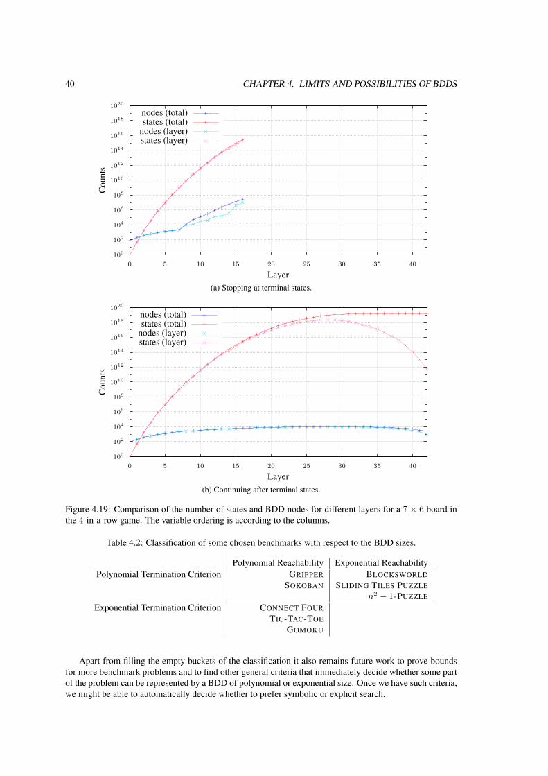
40 CHAPTER 4. LIMITS AND POSSIBILITIES OF BDDS
100
102
104
106
108
1010
1012
1014
1016
1018
1020
0 5 10 15 20 25 30 35 40
Cou
nts
Layer
nodes (total)states (total)
nodes (layer)states (layer)
(a) Stopping at terminal states.
100
102
104
106
108
1010
1012
1014
1016
1018
1020
0 5 10 15 20 25 30 35 40
Cou
nts
Layer
nodes (total)states (total)
nodes (layer)states (layer)
(b) Continuing after terminal states.
Figure 4.19: Comparison of the number of states and BDD nodes for different layers for a 7 × 6 board inthe 4-in-a-row game. The variable ordering is according to the columns.
Table 4.2: Classification of some chosen benchmarks with respect to the BDD sizes.
Polynomial Reachability Exponential ReachabilityPolynomial Termination Criterion GRIPPER BLOCKSWORLD
SOKOBAN SLIDING TILES PUZZLEn2 − 1-PUZZLE
Exponential Termination Criterion CONNECT FOURTIC-TAC-TOE
GOMOKU
Apart from filling the empty buckets of the classification it also remains future work to prove boundsfor more benchmark problems and to find other general criteria that immediately decide whether some partof the problem can be represented by a BDD of polynomial or exponential size. Once we have such criteria,we might be able to automatically decide whether to prefer symbolic or explicit search.

Part II
Action Planning
41


Chapter 5
Introduction to Action Planning
Awaiting my last breaththe mirror calls my nameit’s showing me the wayinto the darkthe bridge appearsI jump into the dark sideand hear the voice it’s cold as ice“Welcome to reality”
Blind Guardian, Lost in the Twilight Hallfrom the Album Tales from the Twilight World
Action planning is a special case of general problem solving, and as such it is an important part of re-search in artificial intelligence. The problem solvers (in this context called planners) need to find a solutionfor the problem at hand without interaction of a human being and also without prior knowledge of the givenproblem. Thus, the developer of such a planner cannot insert any domain-dependent improvements.
All the problems are specified in a common format, which the planners must analyze in order to un-derstand the dynamics. Typical examples for such inputs are STRIPS (Stanford Research Institute ProblemSolver) by Fikes and Nilsson (1971) and PDDL (Planning Domain Definition Language) by McDermott(1998). The latter allows for a more natural description of the desired problems, so that it is now the mostcommonly used language for describing planning problems, especially in the course of the InternationalPlanning Competition (IPC), which is held every second or third year since 1998.
These inputs correspond to an implicit description of a state space. Thus, a planning problem consistsat least of the elements described in Definition 1.4 on page 4, though they are often called somewhatdifferently. In the most basic form we are given a set of fluents or predicates needed to describe a state, anumber of operators (in the context of planning also called actions) to transform states to their successors,an initial state, and a set of terminal states (in planning typically called goal states). The planners are thensupposed to find a solution (in this context called a plan), which corresponds to a sequence of actions thattransforms the initial state to one of the goal states.
In action planning we distinguish several different subareas (called tracks). While this basic idea stillholds in most of these various tracks, some are more complex by specifying further inputs or further restric-tions for a plan.
In the following (Section 5.1) we will give some insight into a number of the different tracks that areoften part of the planning competition as well as to PDDL (Section 5.2). In the following chapters wewill provide algorithms for optimally solving problems from two of the tracks, namely classical planning(Chapter 6) and net-benefit planning (Chapter 7).
43

44 CHAPTER 5. INTRODUCTION TO ACTION PLANNING
5.1 Planning Tracks
There are a number of different planning tracks, e. g., classical planning, over-subscription planning, net-benefit planning, non-deterministic planning, and temporal planning, to name but a few. The core idea issimilar for all of these, though the descriptions as well as the plans—or policies, as the solution of a non-deterministic planning problem is typically called—can vary significantly. Furthermore, in most of thesetracks we distinguish between optimal and satisficing planning. In the former we are interested in findingplans optimal according to some optimization criterion depending on the precise problem at hand, while inthe latter we are interested in finding a legal, not necessarily optimal, plan, though it should be as good aspossible according to the same optimization criterion given certain time and memory constraints.
In classical planning we are provided a number of actions, consisting of preconditions and effects. Anaction can be applied in a state if the precondition is satisfied. In that case, the effect is evaluated to updatethe state. The plan is a sequence of the available actions that, executed one after the other, transform theinitial state to one of the goal states. The optimization criterion is the length of the plan, i. e., the number ofactions it consists of (the fewer the better). If action costs are defined the total cost of the plan, i. e., the sumof the costs of all the actions within the plan, is to be minimized.
Over-subscription planning (or preference planning) allows for preferences or soft goals, i. e., we canspecify which additional fluents we would like to achieve when a goal state is reached. The achievedpreferences then give a certain reward (called benefit or utility). Here, we are typically interested in findinga plan to satisfy a goal that gives the maximal utility. If we also take the length of the plan or its total costinto account, we speak of net-benefit planning, where the net-benefit, which is the achieved utility minusthe cost of the plan needed to achieve it, is to be maximized.
In case of non-deterministic planning we only know the possible effects that might occur when an actionis applied, but not exactly which of these will actually happen. Thus, the solution here consists of findinga policy, which specifies the action to choose in every state that might be reached. Following Cimatti et al.(2003) we distinguish three kinds of policies. A strong one will enable us to reach a goal state, no matterwhat happens due to non-determinism. A strong-cyclic solution corresponds to a policy that allows usto reach a plan if we can wait for an unbounded number of steps, i. e., it might happen that due to non-determinism we end up running in circles, but in the limit we expect due to a fairness condition that thenon-determinism will not always choose the effects in such a way that we remain on the circle and thus willbe able to reach a goal state. Finally, a weak policy allows us to reach a goal state if the non-determinismdoes not play against us. Of course, not all problems allow for a strong or strong-cyclic solution. However,a weak policy should always be possible to find.
Adding a probability for the occurrence of any of the possible effects results in probabilistic planning,where we are interested in finding policies that reach a goal state with the highest probability possible. Un-certainty about the initial state, i. e., a number of possible initial states, is another form of non-determinismand introduced in conformant planning. Here, the planner aims at finding a policy that works for any of thepossible initial states and reaches a goal state.
The idea of temporal planning is the possibility of executing some actions in parallel if they operate ondisjoint resources. Furthermore, the actionsf have a certain duration and the aim is to find a solution thatminimizes the makespan, which is the time needed from the initial state until the last action is finished.
In this work we are only interested in classical and net-benefit planning. For these, we provide ap-proaches to find optimal plans using symbolic search.
5.2 The Planning Domain Definition Language PDDL
For automatic planners to be able to handle planning problems it is important to have a unified language.Currently, the Planning Domain Definition Language PDDL is the language of choice in most planningtracks. Starting with a brief overview of the history of PDDL (Section 5.2.1) we continue with an introduc-tion to the structure of a typical PDDL description along the running example in Section 5.2.2.

5.2. THE PLANNING DOMAIN DEFINITION LANGUAGE PDDL 45
5.2.1 The History of PDDL
Though PDDL is currently the language of choice in action planning, it is not the first approach to a unifiedlanguage for describing planning problems. In this section we will briefly outline the history of such unifiedlanguages and also the evolution of PDDL.
STRIPS
One of the first approaches came with the Stanford Research Institute Problem Solver (STRIPS) by Fikesand Nilsson (1971), whose input language was later also called STRIPS.
A STRIPS description is essentially a four-tupleP = ⟨V,A, I,G⟩with V being a set of binary variables,A a set of actions, I the initial state and G a set of goal states. In STRIPS a state is described by the variablesthat are currently true, i. e., the closed world assumption holds, so that all variables in V that are not part ofthe state are assumed to be false.
The initial state description I ⊆ V thus fully specifies the state where the planning process starts.The goal states G ⊆ V are described by a partial state description, so that the variables within G must
be true in a given state for it to be a goal state, while the other variables may take any value, i. e., a state sis a goal state if G ⊆ s.
An action a ∈ A is tuple a = ⟨prea, adda, dela⟩. The precondition prea ⊆ V is a partial state descrip-tion similar to the goal states G, so that an action a is applicable in the current state s if the precondition’svariables are true in s (i. e., if prea ⊆ s). The effects, i. e., the changes to the current state, of an action a aredescribed by adda and dela. The add-effects adda ⊆ V contain all variables that will be made true afterapplication of the action, the delete-effects dela ⊆ V those that will be made false afterward. The frame,i. e., the set of variables that do not change, is not modeled explicitly. All variables not in adda∪dela retaintheir value. Let s be the current state with prea ⊆ s, so that action a is applicable. Then the successor states′ is specified by the set of variables s′ = (s \ dela) ∪ adda.
Even though STRIPS is a rather restricted approach the decision if a plan can be found for a givenproblem is PSPACE-complete (Bylander, 1994).
ADL
Another approach at a unified language is the Action Description Language (ADL) by Pednault (1989,1994). Using ADL, planning problems can be described in a more concise way than with STRIPS.
There are a number of differences between ADL and STRIPS, starting at the way states are represented.While in STRIPS a state is a set of binary variables (those that are currently true), in ADL a state is fullydescribed by binary facts and their values. Additionally, in ADL an open world is assumed so that any factwhose value is not explicitly stated has an unknown value (not false as in the case of STRIPS). Furthermore,the formulas in the preconditions and the description of the goal states can be more complex. While STRIPSsupports only sets of variables (which can be translated to conjunctions of positive facts in ADL), hereliterals (positive and negative facts) and disjunctions are supported as well. Additionally, (existential anduniversal) quantifications can be used in the formulas. The effects only allow for conjunctions of literals aswell as universal quantifications; a disjunction in an effect would mean that the outcome of an action is notentirely certain.
Another important extension is the use of conditional effects. A conditional effect can greatly decreasethe size of a planning description as it can distinguish the effects an action has depending on the state it isapplied in, i. e., a conditional effect can be seen as an action within an action. It consists of an antecedent(the precondition of the sub-action), which may be a Boolean formula in the same way a normal action’sprecondition is, and a consequence, which describes the additional effects that take place if the antecedentis satisfied in the current state.
Though the language seems more powerful, actually it is possible to translate planning problems de-scribed in ADL to ones described in STRIPS (Gazen and Knoblock, 1997; Hoffmann et al., 2006).
A first step in such a translation is to transform the description of the goal states G to an action with theprecondition being G and the only effect the addition of a new variable goal -achieved to the current state.Thus, the goal states are reached once the variable goal -achieved is present in the current state.

46 CHAPTER 5. INTRODUCTION TO ACTION PLANNING
The conditional effects are what make things most difficult. For a conditional effect in an action itis possible to generate two actions, one for the case that the conditional effect is applicable, one for thecase that it is not. Thus, the first action’s precondition is the conjunction of the original action’s precon-dition with the conditional effect’s antecedent, while the effects are the conjunction of the original effectswith the consequence of the conditional effect. The second action’s precondition is the conjunction of theoriginal precondition with the negation of the conditional effect’s antecedent, while the effects remain un-changed—if the conditional effect is not applicable in the current state then it will not change anythingabout that state. This process can be iterated until no conditional effects are present anymore in any action.For one action the resulting description contains a number of actions exponential in the number of condi-tional effects in the original action. Nebel (1999, 2000) proved that it is not possible to come up with ashorter STRIPS description.
The quantifiers can be expanded using the constants that might replace the quantified variables, so thatthey result in a number of disjunctions in case of existential quantifiers or conjunctions in case of universalquantifiers.
By calculating the disjunctive normal form (DNF) of an action’s precondition the result is a disjunctionof conjunctions of literals. This way it is possible to split the action into a number of smaller actionscontaining the same effects but different preconditions—one for each operand of the disjunction.
Finally, to remove the negations within the actions’ preconditions it is best to establish negation normalform (NNF), which is immediate if in the last step the DNF was created. In NNF any negations appear onlyimmediately in front of a fact. For such a negated fact fac an additional (positive) fact not-fac is insertedto represent the negation of fac, so that it must always take the opposite value of fac. Thus, if fac holds inthe initial state I not-fac must not and vice versa. Also, whenever the value of fac is changed in an action,so must the value of not-fac, i. e., if fac is an add effect then not-fac must be a delete effect and vice versa.Any appearance of the negated fac in a precondition is replaced by the (non-negated) not-fac.
All in all, as problems in ADL can be translated into equivalent problems in STRIPS the decisionproblem if a plan exists in an ADL description is also PSPACE-complete.
PDDL
Finally, the Planning Domain Definition Language (PDDL) was proposed by McDermott (1998) to be onthe middle-ground between STRIPS and ADL. In a PDDL description it is possible to specify a numberof requirements a planner must be able to handle in order to correctly work with this description. Therequirements range from pure STRIPS to full ADL. Some of them are the following:
:strips Basic STRIPS add and delete effects (by means of a conjunction of positive and negative facts)should be used.
:disjunctive-preconditions Preconditions can contain disjunctions.
:existential-preconditions Preconditions can contain existential quantifications.
:universal-preconditions Preconditions can contain universal quantifications.
:quantified-preconditions Preconditions may contain any kind (existential or universal) of quantifications.
:conditional-effect The effects may contain conditional effects.
:adl A meta-requirement that encapsulates all of the above.
A PDDL description consists of two parts (typically stored in separate files), the domain descriptionand the problem description. The domain description specifies the general behavior, while the problemdescription determines the precise objects that can appear in the problem at hand. In more detail, thedomain description is mainly concerned with the actions, in many cases independent of the actual factspresent. The problem description is concerned with the problem-dependent initial state and goal states aswell as the actual objects—constants for replacing possible variables within the action descriptions—thatmust be handled.

5.2. THE PLANNING DOMAIN DEFINITION LANGUAGE PDDL 47
In many cases the domain description does not contain any specific facts but is modeled using a numberof variables. When bringing a domain and a problem description together these variables can be replaced bythe actual objects, i. e., the planning description can be instantiated (or grounded) for easier reasoning (see,e. g., Edelkamp and Helmert, 1999; Helmert, 2008). Using this instantiation and the rules for translatingADL to STRIPS from the previous section it is possible to transform a PDDL description so that it equals aSTRIPS description.
PDDL was extended to handle numerical variables and a concurrent execution of actions by Fox andLong (2003) resulting in PDDL 2.1, which is divided into three different levels.
Classical Planning The idea behind classical planning is essentially the same as in the original PDDLspecification, i. e., states are considered as being the conjunction of positive or negative facts and aplan consists of a sequence of actions that transforms the initial state to one of the goal states.
Metric Planning In metric planning numbers are added in form of the real-valued numerical variables. Theclassical planning state is extended to allow for simple arithmetic expressions using these variables.Such expressions might be the addition, subtraction or assignment of a constant or another numericalvariable.
Temporal Planning To handle temporal planning problems, durative actions were added. These actionscontain a duration, but may also have certain conditions holding at specified points of time. Espe-cially, the preconditions are transformed to conditions at some time point. If this time point is at thestart of the action it corresponds to a classical precondition.
The effects might also take place at different points of time. So it might be possible to create actionsthat result in some effect immediately after the action has been started, but also in other effects thattake place sometime later, e. g., once the action has ended.
The goal is to find a plan that executes the actions in such an order (possibly some even in parallel),so that a goal state is reached after the shortest possible time.
After that PDDL was further extended. In PDDL 2.2 (Hoffmann and Edelkamp, 2005) so called derivedpredicates were integrated. These are great for decreasing the size of a description, as they might be seenas utility functions. Each derived predicate depends on other facts or derived predicates. It is simply a shortway to describe some aspects of the planning state, somewhat similar to functions in programming, whichencapsulate code that can be used in several locations within other functions.
Another extension introduced with PDDL 2.2 were timed initial literals. These are facts that are set to acertain value (true or false) at some predetermined point of time. This is done automatically without callingany action. Of course, this extension is only needed for temporal planning.
The next step in the development of PDDL was the proposal of PDDL 3.0 (Gerevini and Long, 2005,2006). The new version now also included the definition of constraints and preferences. The first ones areused to constraint the set of plans (using a temporal logic to describe them) while the latter ones are usedto express soft constraints. These constraints are not mandatory to be satisfied, but if they are not the plan’squality will decrease.
Finally, in the context of the sixth International Planning Competition (IPC) 2008 PDDL 3.110 wasproposed. It allows to define functional variables, which can no longer only be true or false (classicalplanning) or numerical (metric planning), but can be of any finite domain. Especially it is possible to modelvariables whose domains are other objects of the domain. In principle, this is designed according to theSTRIPS extension allowing for functional state variables (Geffner, 2000).
5.2.2 Structure of a PDDL DescriptionIn the following we will show how a PDDL description is organized. For this we will show the importantparts of the domain and problem descriptions for our running example introduced in Section 1.6. In thisdomain we are confronted with a desert, consisting of a number of locations between which the gunslinger
10http://ipc.informatik.uni-freiburg.de/PddlExtension; the BNF description of it is due to Kovacs (2011)

48 CHAPTER 5. INTRODUCTION TO ACTION PLANNING
p1
p2
p3 p6
p8
p9
p7
p5
p4
p0mibgunslinger
Figure 5.1: The running example in classical planning with unit-cost actions. The optimal solution isdenoted by the thicker edges.
can move. The goal for the gunslinger is to reach the man in black at the end of the desert (position p9),who cannot move in this setting.
We will discuss the structure of the domain and the problem along this example in the context of classicalplanning with unit-cost actions. The changes needed for classical planning with general action costs aswell as for net-benefit planning will be described in the corresponding chapters. The complete PDDLdescriptions for all three can be found in Appendix A.
Here we assume the situation as in Figure 5.1. We have the same desert as before with locations p0 top9, some of which are connected, so that the protagonist can move from one location to an adjacent one.In this case the protagonist is the gunslinger, which starts at location p0, the entrance to the desert. Asclassical planning does not use an opponent, the man in black (mib) is static at location p9, the exit fromthe desert. The goal is to move the gunslinger from p0 to the location where the man in black hides and tocatch him there using as few actions as possible.
The domain description (cf. Figure 5.2) stores all the information concerning the predicates as well asthe actions. It starts with the specification of the domain’s name—(domain <domain-name>).
Next, some requirements are stated. The first one, :strips, means that we can use only conjunctionsin the actions’ preconditions as well as the goal description and the effects are in STRIPS style, i. e., a set ofadd-and delete-effects. The :typing requirement means that we can have different types, so that certainobjects can replace only those variables of a predicate that have the same type.
After these the types are specified. In this case we use two types, one—person—to denote the peo-ple running through the desert, the second one—location—to denote the possible locations within thedesert.
Following these, some constants may be specified. These essentially can be used to replace variablesof the same type. Typically, we need constants (or objects) in the problem description to specify a certaininstance of the domain at hand. Here, we know that no matter what the desert might look like we have onlytwo people, the gunslinger and the man in black (mib).
Then, a list of all predicates in the domain is given, along with their (typed) parameters. The parametersare given in form of variables, which in PDDL are always denoted by the prefix ?. In this example we havethree different predicates—the two-ary position, which denotes the location the corresponding personis currently in, the two-ary adjacent relation, which denotes which locations are next to each other andcan thus be reached by a single move, and the 0-ary caughtMIB, which denotes whether the man in blackhas been caught or not.
Finally, the list of all the actions is given. Each action consists of the action’s name, a list of (typed) pa-rameters, the precondition, and the effect. While in principle the precondition might be an arbitrary formula,given the necessary requirements, in this example we are only allowed to use conjunctions of predicates.The effects are STRIPS-like, i. e., they represent the add-and delete-lists by being simple conjunctions ofpositive (add) or negative (delete) predicates.

5.2. THE PLANNING DOMAIN DEFINITION LANGUAGE PDDL 49
(define (domain desertClassic)(:requirements :typing)(:types person location)(:constants
gunslinger mib - person)(:predicates
(position ?p - person ?l - location)(adjacent ?l1 ?l2 - location)(caughtMIB)
)
(:action move:parameters (?l1 ?l2 - location):precondition(and
(position gunslinger ?l1)(adjacent ?l1 ?l2)
):effect(and
(not (position gunslinger ?l1))(position gunslinger ?l2)
))
(:action catchMIB:parameters (?l - location):precondition(and
(position gunslinger ?l)(position mib ?l)
):effect(caughtMIB)
))
Figure 5.2: The domain description for the classical planning version with unit-cost actions of the runningexample.
The first action—move—allows the gunslinger to move from one location to an adjacent one. If thegunslinger is currently at some location ?l1 he can move to an adjacent location ?l2. If he does, the effectsimply states that he is no longer at location ?l1 but rather at location ?l2.
The second action—catchMIB—allows the gunslinger to actually catch the man in black. He can dothis if he has reached a location ?l, which must be the same as the location where the man in black resides.If he decides to catch the man in black, the predicate caughtMIB is set to true, while no other predicatesare affected.
The problem description (cf. Figure 5.3) captures all the stuff needed to generate one instance of thedomain at hand, i. e., the objects to replace the variables from the definitions in the domain description, theinitial state, and the specification of the goal states.

50 CHAPTER 5. INTRODUCTION TO ACTION PLANNING
(define (problem desertClassicProb)(:domain desertClassic)(:objects
p0 p1 p2 p3 p4 p5 p6 p7 p8 p9 - location)
(:init(position gunslinger p0)(position mib p9)(adjacent p0 p1) (adjacent p1 p0)(adjacent p0 p2) (adjacent p2 p0)(adjacent p0 p3) (adjacent p3 p0)(adjacent p1 p3) (adjacent p3 p1)(adjacent p1 p4) (adjacent p4 p1)(adjacent p2 p3) (adjacent p3 p2)(adjacent p2 p5) (adjacent p5 p2)(adjacent p3 p4) (adjacent p4 p3)(adjacent p3 p5) (adjacent p5 p3)(adjacent p3 p6) (adjacent p6 p3)(adjacent p4 p6) (adjacent p6 p4)(adjacent p4 p7) (adjacent p7 p4)(adjacent p5 p6) (adjacent p6 p5)(adjacent p5 p8) (adjacent p8 p5)(adjacent p6 p7) (adjacent p7 p6)(adjacent p6 p8) (adjacent p8 p6)(adjacent p6 p9) (adjacent p9 p6)(adjacent p7 p9) (adjacent p9 p7)(adjacent p8 p9) (adjacent p9 p8)
)
(:goal(caughtMIB)
))
Figure 5.3: The problem description for the classical planning version with unit-cost actions of the runningexample.
It starts by specifying a name for the problem—(problem <problem-name>)—and a referenceto the corresponding domain—(:domain <domain-name>). The domain name mentioned here mustequal the one in the domain description.
Next, some objects may be defined. These objects are similar to the constants of the domain descriptionin that they can be inserted as the arguments of certain predicates, but they may not be used in the domaindescription, only in the problem description, as they build the basis for this specific instance. If the corre-sponding requirement is set in the domain description, these objects may be typed. In the example the onlyobjects are the ten locations p0 to p9.
After that, the initial state is specified. In this, no variables are allowed. Also, a closed world assumptionis made, i. e., any predicate not listed here is supposed to be false in the initial state. Apart from the positionsof the gunslinger and the man in black it also captures all the information concerning the adjacency of thelocations.
Finally, the goal is specified. In this example, it is only a single predicate, denoting that the man inblack has been caught. In principle, PDDL supports arbitrary formulas as well, but the correspondingrequirements must be set in the domain description.

5.2. THE PLANNING DOMAIN DEFINITION LANGUAGE PDDL 51
In classical planning we are typically interested in finding a plan which contains as few actions aspossible. Thus, in this case we must find the shortest path from p0 to p9 and then immediately catch theman in black. Though a plan bringing the gunslinger from p0 to p9, moving it further to p7 and back top9 before finally catching the man in black is valid, it is clearly not the optimal one and thus the other oneshould be generated.
Here, the shortest path is simply following the straight line from the left to the right. In other words, theoptimal plan is
0: (move p0 p3)1: (move p3 p6)2: (move p6 p9)3: (catchMIB p9)
which we have also depicted by the thicker edges in Figure 5.1.

52 CHAPTER 5. INTRODUCTION TO ACTION PLANNING

Chapter 6
Classical Planning
I love it when a plan comes together.
Col. John “Hannibal” Smith in The A-Team
In classical planning we are confronted with structurally rather simple planning problems. All we getare descriptions of the initial state, the goal states and the available actions. Based on these we want to finda plan containing as few actions as possible (in case of unit-cost actions, or if no costs are specified at all) orwhose total cost is as small as possible (in case of more general action costs) (see, e. g., Russell and Norvig,2010; Edelkamp and Schrodl, 2012).
Definition 6.1 (Classical Planning Problem). A classical planning problem is described by a tuple P =⟨V,A, I,G, C⟩ with V being the variables that build a state11, A a set of actions consisting of preconditionand effects (i. e., an action a ∈ A is given by a pair ⟨prea, eff a⟩), I an initial state, G a set of goal states,and C : A →→ N+
0 a cost function specifying a certain non-negative integral cost for each action in A.12 Insome domains C might be omitted. In this case all actions are supposed to have a unit cost of 1. Thus, evenwhen no action costs are specified we speak of unit-cost actions, whereas we speak of general action costsif at least two actions have different costs.
While the PDDL specification allows only for binary variables, it is possible to find sets of mutuallyexclusive variables, i. e., sets of binary variables of which at most one can hold at any time. Thus, V can alsobe viewed as a set of multi-valued variables. This setting is often refered to as SAS+ planning (Backstromand Nebel, 1995).
Definition 6.2 (Plan). A plan is a sequence of actions π = (A1, A2, . . . , Am) ∈ Am whose application,starting at I, results in a goal state, i. e., Am (Am−1 (. . . A1 (I) . . . )) ∈ G.
Definition 6.3 (Cost of a Plan). The total cost C (π) of a plan π = (A1, . . . , An) is the sum of the costs ofall actions within π, i. e., C (π) := C (A1) + C (A2) + · · ·+ C (An).
Note that in case of unit-cost actions the cost of the plan actually corresponds to the number of actionswithin the plan.
Definition 6.4 (Optimal Plan). A plan π is called optimal, if there is no plan π′ with C (π′) < C (π).
We can model a classical planning problem as a directed graph with nodes u corresponding to the statesand edges e = (u, v) corresponding to the actions leading from u to v. One of those nodes, the root node,corresponds to the initial state and a subset of them, the terminal nodes, to the goal states. A plan thencorresponds to a path from the root to a terminal node. If we are confronted with general action costs, these
11In case of PDDL these are given in terms of the predicates as well as the constants and objects defined to replace the variableswithin the predicates.
12In the actual planning descriptions the costs are typically non-negative rational numbers, which we can scale to integer values.
53

54 CHAPTER 6. CLASSICAL PLANNING
Algorithm 6.1: Symbolic Breadth-First SearchInput: Planning problem P = ⟨V,A, I,G⟩.Output: Step-optimal plan or “no plan”.
1 reach0 ← I // First layer contains only I.2 closed ← ⊥ // So far, no states expanded.3 layer ← 0 // Initial layer’s index is 0.4 while reach layer ∧ G = ⊥ do // Repeat until goal state found.5 reach layer ← reach layer ∧ ¬closed // Before expansion, remove states already expanded.6 if reach layer = ⊥ then return “no plan” // If no new states left to expand, return “no plan”.7 closed ← closed ∨ reach layer // Add new states to set of all expanded states.8 reach layer+1 ← image (reach layer ) // Calculate successor states.9 layer ← layer + 1 // Increase layer’s index for next iteration.
10 reach layer ← reach layer ∧ G // Retain only reached goal states in final layer.11 return RetrieveBFS (P, reach, layer) // Retrieve plan and return it.
can be modeled by inserting edge weights, so that the cost of a plan in this scenario equals the sum of theweights of the edges taken by the corresponding path, while in case of unit-cost actions the cost correspondsto the length of the path. An optimal plan is a path with minimal total weight (or length).
In this chapter we will show how to optimally solve classical planning problems by symbolic searchalgorithms. In Section 6.1 we introduce algorithms for solving problems with unit-cost actions, while inSection 6.2 we deal with general action costs. For the latter we typically need some heuristic to provide anestimate on the minimal cost required to reach a goal state from each reachable state. We briefly introducesome of the most commonly used heuristics as well as the one we use, namely pattern databases, in Section6.3. Afterward we describe how we implemented our planner, called GAMER, along with a number ofimprovements to the algorithms (Section 6.4) before we provide some experimental results, some of those ofthe International Planning Competitions in 2008 and 2011, some for evaluating our improvements (Section6.5).
6.1 Step-Optimal Classical PlanningWe start with rather simple symbolic algorithms that solve classical planning problems with unit-cost ac-tions optimally. In other words, they find a plan containing the minimal number of actions.
6.1.1 Symbolic Breadth-First SearchThere are several approaches to find step-optimal plans, e. g., breadth-first search (BFS), depth-first search(DFS), and iterative-deepening depth-first search (ID-DFS) to name but a few. We are only interested inalgorithms efficiently utilizing BDDs, so the easiest approach is to perform a BFS starting at the initial stateI and stopping once a goal state g ∈ G is found.
As we have seen in Chapter 3, in symbolic search such a BFS is easy to implement. All we need to dois iterate the image calculations until the BDD representing the current BFS layer contains at least one goalstate. To be able to retrieve a plan we store all BFS layers in separate BDDs reach layer (cf. Algorithm 6.1).In order to guarantee termination in case of no existing plan we store the set of all states expanded so far inthe BDD closed , so that we can stop the search when we have found all states without ever reaching a goalstate, i. e., when the layer to be expanded next contains only states already expanded before. In that case wereturn the text “no plan”.
Retrieval of a Plan
Given the BDDs for all the BFS layers, the last of which contains the first reached goal states, and the indexof the last layer n, we want to compute an optimal plan containing n actions. In order to determine this

6.1. STEP-OPTIMAL CLASSICAL PLANNING 55
Algorithm 6.2: Retrieval of a Plan for Symbolic BFS (RetrieveBFS )Input: Planning problem P = ⟨V,A, I,G⟩.Input: Set of BDDs reach representing the BFS layers.Input: Index n of layer containing goal states.Output: Step-optimal plan π.
1 π ← () // Plan is initially empty.2 current ← reachn // Start with the states in the final layer.3 for layer ← n to 1 do // Iterate through all layers, in reverse order.4 for all a ∈ |A| do // Iterate through all actions.5 pred ← pre-imagea (current) // Calculate predecessors of current states.6 if pred ∧ reach layer−1 = ⊥ then // If some predecessors are within previous layer. . .7 current ← pred ∧ reach layer−1 // Retain only predecessor states also in previous layer.8 add action a to the front of π // Store current action in the plan.9 break // Ignore remaining actions.
10 return π // Return the generated plan.
I Gn
(a) Unidirectional.
n1 n2
I G
(b) Bidirectional.
Figure 6.1: The search spaces of uni- and bidirectional BFS.
plan we must know which actions to take, so that the normal pre-image operator cannot be used, becausethat operates over all actions. Instead we apply the single-operator pre-image operator pre-imagea (cf.Definition 3.7 on page 21) for each action a ∈ A.
The pseudo-code for the retrieval is provided in Algorithm 6.2. We start at the reached goal states inlayer n and apply the single-operator pre-image operator for one action after the other. Once one suchpre-image results in a set of predecessor states of which some are part of the previous BFS layer reachedin forward direction (line 6) we use those as the new starting point and switch to the previous layer. Werepeat these steps until finally we reach the initial state (the only one in layer 0). Store all the found actionsin reverse order results in a plan of optimal length.
6.1.2 Symbolic Bidirectional Breadth-First Search
During the experiments with several of the older IPC domains we found some for which forward search isfaster than backward search, others where both are of similar speed, and some for which backward searchis the faster approach. To automatically decide whether to prefer forward or backward search we alsoimplemented a bidirectional BFS. In it we have two search frontiers, one starting at the initial state I, theother one starting at the goal states G. These frontiers are extended by using the image and the pre-imageoperator, respectively, until they overlap (cf. Figure 6.1).

56 CHAPTER 6. CLASSICAL PLANNING
Algorithm 6.3: Symbolic Bidirectional Breadth-First SearchInput: Planning problem P = ⟨V,A, I,G⟩.Output: Step-optimal plan or “no plan”.
1 freach0 ← I // First (forward) layer contains only I.2 breach0 ← G // First backward layer contains all goal states G.3 fclosed ← bclosed ← ⊥ // So far, no states expanded in either direction.4 flayer ← blayer ← 0 // Indices of forward and backward layers, both starting at 0.5 ftime ← btime ← 0 // Forward and backward runtime initialized to 0.6 while freachflayer ∧ breachblayer = ⊥ do // Repeat until forward and backward layers overlap.7 if ftime ≤ btime then // Perform forward step.8 perform one step of Symbolic BFS in forward direction. // Lines 5 to 9 in Algorithm 6.1.9 update ftime // Store time for this forward step.
10 else // Perform backward step.11 perform one step of Symbolic BFS in backward direction. // Lines 5 to 9 in Algorithm 6.1.12 update btime // Store time for this backward step.
13 freachflayer ← breachblayer ← freachflayer ∧ breachblayer // Retain only states from the// intersection of forward and backward frontier in the final layers.
14 return RetrieveBBFS (P, freach,flayer , breach, blayer) // Retrieve plan and return it.
In the pseudocode (cf. Algorithm 6.3) we keep track of the BFS layers, the set of expanded states, theindex of the current layer and the time of the last step in forward direction (freach , fclosed , flayer , andftime) as well as in backward direction (breach , bclosed , blayer , and btime). Every step corresponds toa step in unidirectional BFS (lines 5 to 9 in Algorithm 6.1), but in backward direction we must use thepre-image instead of the image operator. After each step we compare the runtimes for the last forward andbackward steps and continue in the direction where the last step was performed faster. Thus, for problemsthat are easier searched in forward direction the search will be performed mostly forwards and vice versa.
In the bidirectional case we will typically expand a smaller (total) number of states, as we can stop whenthe two search frontiers overlap. In most cases each frontier is a lot smaller than the largest unidirectionalone, so that we end up with a shorter total running time, though this is not necessarily the case. As acounter-example take a problem that is hard in backward direction (e. g., SOKOBAN). Though we mostlyperform forward search, every once in a while we will also perform a backward step. The last of thesebackward steps might very well dominate the total runtime, so that the bidirectional search might actuallytake longer than pure forward search.
Retrieval of a Plan
For the bidirectional case the solution reconstruction is divided into two parts (cf. Algorithm 6.4). At first,it handles the layers generated in forward direction as shown in Algorithm 6.2. Afterward, it starts at theinitial state and applies all the returned actions, resulting in the one state inter of the intersection betweenthe forward and backward layers that is reached using these actions. Then the solution reconstruction forthe backward layers starts. It looks the same only that it is performed in forward direction starting at inter .In the end, both partial plans are concatenated and the resulting overall plan is returned.
6.2 Cost-Optimal Classical PlanningOptimally solving planning problems with general action costs requires more sophisticated algorithms. Anoptimal plan is no longer necessarily one of minimal length but rather one with the minimal total cost, i. e.,the sum of the costs of all actions within the plan must be minimal.
As we have pointed out earlier, in planning the full state space can be seen as a graph G = (V,E,w),with the states being the nodes V of the graph and the actions the connecting edges E, though given inan implicit fashion. An edge’s weight w is thus the corresponding action’s cost. Dijkstra’s single-source

6.2. COST-OPTIMAL CLASSICAL PLANNING 57
Algorithm 6.4: Retrieval of Plan for Symbolic Bidirectional BFS (RetrieveBBFS)Input: Planning problem P = ⟨V,A, I,G⟩.Input: Set of BDDs freach representing the BFS layers found in forward direction.Input: Index n1 of forward layer containing intersection of the two frontiers.Input: Set of BDDs breach representing the BFS layers found in backward direction.Input: Index n2 of backward layer containing intersection of the two frontiers.Output: Step-optimal plan π.
1 perform RetrieveBFS (P, freach, n1) in default direction // Generate plan for forward layers.2 result: π1 = (A1, . . . , An1)3 inter ← I // Start finding intermediate state from I.4 for step ← 1 to n1 do inter ← imageAstep
(inter) // Find intermediate state after performing π1.5 perform RetrieveBFS (P, breach, n2) in reverse direction // Generate plan for backward layers.6 result: π2 = (An1+1, . . . , An1+n2
)7 return π ← (A1, . . . , An1
, An1+1, . . . , An1+n2) // Return combined plans.
shortest-paths search (1959) is one of the classical algorithms used to search for shortest paths in graphswith edge weights. We will introduce it in more detail and provide a symbolic version of it in Section 6.2.2.
The main problem of Dijkstra’s algorithm is that it is blind, i. e., it searches in all directions at once. Toovercome this problem heuristics can be used, which provide an estimate to the distance to a goal state andthus can be used to direct the search, so that fewer states must be expanded in order to find an optimal plan.An extension of Dijkstra’s algorithm that makes use of heuristic estimates is A* search (Hart et al., 1968).In Section 6.2.3 we will introduce a symbolic version of A*.
A* can only work well if we are using a good heuristic, which guides the search in a sensible way.In Section 6.3 we will briefly introduce to a number of heuristics that are often used in action planning,and provide more details to the one we actually use, namely (symbolic) pattern databases (Culberson andSchaeffer, 1998; Edelkamp, 2002b) in Section 6.3.1 and (symbolic) partial pattern databases (Andersonet al., 2007; Edelkamp and Kissmann, 2008d) in Section 6.3.2.
However, before we introduce these possibilities to solve classical planning problems cost-optimally wefirst of all extend the running example from Sections 1.6 and 5.2.2 to this setting in Section 6.2.1 and showhow to adapt the PDDL description accordingly.
6.2.1 Running Example with General Action CostsIn order to extend the running example of the gunslinger following the man in black through the desert tothe setting of general action costs all we need to do is to specify the cost of each action. If some action isdefined without a cost it is treated as a zero-cost action, i. e., an action of cost zero, which does not changethe value of a plan. In this example we assume the costs of the moves from one location to an adjacent oneto be as according to the graphical representation in Figure 6.2.
To extend the PDDL description given in Figures 5.2 and 5.3 in Section 5.2.2 to the setting with gen-eral action costs we need an additional requirement—:action-costs. Furthermore, apart from theobjects and the predicates we must define some functions in the domain description, in this case the onefor calculating the total cost of a plan—total-cost—and also one for specifying the cost for eachmove—moveCost:
(:functions(total-cost) - number(moveCost ?l1 ?l2 - location) - number
)
The latter we need to keep the domain description independent of the actual instance, as we can definethe move costs in the initial state. Both functions are of type number, so that we can use arithmeticoperators such as comparisons or assignments. In this case, we must only specify the initial values in theinitial state, e. g., (= (total-cost) 0) (and similarly specify the costs for all the edges by using the

58 CHAPTER 6. CLASSICAL PLANNING
p1
p2
p3 p6
p8
p9
p7
p5
p4
p0
2
10
1 4
2
7 5
3
101
312
2 7
7
3 6 1
13gunslinger mib
Figure 6.2: The running example in classical planning with general action costs. The optimal solution isdenoted by the thicker edges.
moveCost function), and the increase of the total-cost in the effect of each action, e. g., (increase(total-cost) (moveCost ?l1 ?l2)). In this example, we do not specify any cost for catchingthe man in black, so that this action can be performed without influencing the overall cost of the plan.
Apart from the initialization of the total action costs and the move costs for the adjacent locations wealso need a metric in the problem description. In this case, it only says to minimize the total action costs:
(:metric minimize (total-cost))
The full PDDL description can be found in the appendix of this thesis (Section A.2).In this setting an optimal solution has a total cost of 14 and uses a total of eight actions:
0: (move p0 p1) [2]1: (move p1 p3) [2]2: (move p3 p5) [2]3: (move p5 p8) [3]4: (move p8 p6) [1]5: (move p6 p7) [1]6: (move p7 p9) [3]7: (catchMIB p9) [0]
The square brackets denote the costs of the actions. This solution is also depicted in Figure 6.2 by use ofthe thicker edges.
6.2.2 Symbolic Dijkstra SearchThe general idea of Dijkstra’s single-source shortest-paths algorithm (1959) in the setting of graph searchis to find each node’s minimal distance g from the root node. It starts with the root node and then alwaysexpands a node u with minimal distance g (u) from the root among all unexpanded nodes. After expansionthe distances of the successors of u are updated in order to reflect that a path along that node might becheaper than another path along which it was reached before, i. e., for each v with (u, v) ∈ E the distancefrom the root node is set to
g (v) = min g (v) , g (u) + w (u, v) , (6.1)
with w (u, v) being the weight of the edge (u, v).The algorithm is usually performed by using a priority queue. A priority queue stores data along with
a certain priority. In this context we need two functions, deleteMin and decreaseKey . The former allowsus to remove the date with minimal priority, the latter lets us decrease the priority of the specified date. Incase of Dijkstra’s algorithm, the priority queue stores the nodes along with their distance to the root node,interpreted as the priority. Initially, the distance of the root node is 0 and that of the other nodes∞.
The node u to be expanded next is the one with minimal distance g (u), which is returned by callingthe priority queue’s deleteMin function. The priorities of all nodes that can be reached from u must be

6.2. COST-OPTIMAL CLASSICAL PLANNING 59
Algorithm 6.5: Symbolic Version of Dijkstra’s AlgorithmInput: Planning problem P = ⟨V,A, I,G, C⟩.Output: Cost-optimal plan or “no plan”.
1 open0 ← I // I’s total cost is 0.2 closed ← ⊥ // So far, no states expanded.3 g ← 0 // Current total cost is 0.4 while openg ∧ G = ⊥ do // Repeat until a goal state is found.5 openg ← openg ∧ ¬closed // Remove all states already expanded.6 if
gi=g−Cmax+1 openi = ⊥ then // If Cmax consecutive layers are empty. . .
7 return “no plan” // return “no plan”.
8 if openg = ⊥ then // If unexpanded states with total cost g exist. . .9 if zero-cost actions present then perform BFS in openg using only zero-cost actions
10 closed ← closed ∨ openg // Add states to be expanded next to already expanded states.11 for c← 1 to Cmax do // For all (non-zero) action costs c . . .12 openg+c ← openg+c ∨ imagec
openg
// Find successors and add them to the priority queue.
13 g ← g + 1 // Iterate to next total cost.
14 openg ← openg ∧ G // Retain only goal states in final bucket.15 return RetrieveDijkstra (P, open, g) // Retrieve plan and return it.
updated using the decreaseKey function according to equation 6.1 in order to reflect the new knowledge ofthe weight of a path from the root via u to that state.
In our setting we are confronted with an implicit search problem, so that we cannot insert all reachablestates into the priority queue from the start. Instead we use two structures, one being the priority queueopen , which stores the already generated but not yet expanded states, the other the set of all states alreadyexpanded (closed ). As all costs are non-negative and thus the priorities of the states we expand are mono-tonically increasing we can be certain that a state that has been expanded once will not be found on anotherpath with a lower cost. After generation of a successor state we check if it was already expanded, i. e., if itis within the closed list. If it is we can discard the state, otherwise we check for it in the priority queue. If itis present there we might need to update its priority, otherwise we insert it with the corresponding priority.
In the symbolic version of Dijkstra’s algorithm (cf. Algorithm 6.5) we need a way to access the stateshaving a certain total cost from I. This might be done by extending the states by their total costs, i. e., byadding ⌈log n+ 1⌉ additional binary variables if we can be sure that the maximal total cost ever achievableis n, so that the total costs are stored in the BDD representing the set of reachable states. Another possibilityis to partition the priority queue into buckets, resulting in a simple list (Dial, 1969) in which we store allthe states that have been reached so far in the bucket representing the total cost from I that was needed toreach them.
We initialize the priority queue open to contain only I with a total cost of 0. Starting there, we calculateall the successors having a cost of c ∈ 1, . . . , Cmax, with Cmax being the greatest action cost in theproblem at hand. In contrast to the full image or the imagea operator used in the algorithms for retrievinga plan, which contains only the transition relation for one action a ∈ A, the equal-cost image operatorimagec contains all the transition relations for actions with an equal cost of c.
Definition 6.5 (Equal-Cost Image Operator). Given a set of states current , specified in the variable set V ,the successor states resulting from the application of the actions a ∈ A with the same cost c are calculatedby the equal-cost image operator
imagec (current) :=
a∈a|a∈A∧C(a)=c(∃V . T Ra (V,V ′) ∧ current (V)) [V ′ → V]
=
a∈a|a∈A∧C(a)=cimagea (current)

60 CHAPTER 6. CLASSICAL PLANNING
Algorithm 6.6: Retrieval of a Plan for Symbolic Dijkstra (RetrieveDijkstra)Input: Planning problem P = ⟨V,A, I,G, C⟩.Input: Set of BDDs open representing all states reached in forward direction in their corresponding
cost buckets.Input: Total cost g of found goal states.Output: Cost-optimal plan π.
1 π ← () // Initial plan is empty.2 current ← openg // Start with final bucket.3 while I ∧ current = ⊥ do // Repeat, until I is reached.4 if zero-cost actions present then retrieve BFS plan in openg using only zero-cost actions5 for c← Cmax to 1 do // For all possible costs c. . .6 for all a ∈ A with C (a) = c do // For all actions a with cost c. . .7 pred ← pre-imagea (current) // Calculate predecessors using action a.8 if openg−c ∧ pred = ⊥ then // If predecessor has total cost of g − c. . .9 current ← openg−c ∧ pred // Take predecessors as current states.
10 add action a to front of plan π // Extend plan by found action.11 g ← g − c // Update index of cost layer for next iteration.12 goto line 3 // Continue in predecessor’s bucket.
13 return π // Return the complete plan.
We add the successors to the priority queue (line 12) into their corresponding buckets by calculating thedisjunction with the BDD representing the states already in that bucket. In case some bucket does not yetexist in the priority queue, instead of calculating the disjunction with the BDD stored at that bucket we needto create the required bucket and insert a new BDD consisting only of the successors.
For the closed list a single BDD closed is sufficient. It is initially empty (line 2) and new states areinserted when they are expanded (line 10). Before actually expanding some bucket the already expandedstates are removed (line 5) in order to prevent expanding any state twice.
The search ends when a goal state has been found (line 4). In that case the last bucket is updated tocontain only the goal states in preparation of the retrieval of a plan. In problems where no plan can be foundthe search also terminates when Cmax consecutive buckets are empty (line 6). In that case all states havebeen expanded because the action costs are at most Cmax so that any successor must reside in one of thenext Cmax buckets.
If actions with a cost of 0 are present the algorithm gets more complicated. The problem is that theirsuccessors reside in the same bucket as the states being expanded, so that this bucket must be expandedseveral times. To prevent this we start a BFS using only the zero-cost actions for the bucket to be expandednext (line 9) and afterward expand all states reached in this BFS to generate the successors in other buckets.Note that in order to retrieve the full plan the layers of the BFS should be stored within the bucket, so thatwe actually need a two-dimensional structure.
Retrieval of a plan
If we can keep the complete priority queue in main memory the final calculation of the plan works as shownin Algorithm 6.6. We start at the bucket in which a goal state was found (line 2). From this we determinethe predecessors starting with the actions with highest cost and check if one is present in the correspondingbucket (line 8). If it is we continue with the predecessor states in that bucket (line 9), otherwise we checkthe actions with smaller cost. This we iterate until the initial state I is reached (line 3).
In case of zero-cost actions the retrieval gets more complicated as well. Before calculating the prede-cessors of a bucket we must first of all find a plan within the bucket, i. e., along the BFS layers calculated inforward direction, that transforms a state from the first layer within this bucket to one of the current states.

6.2. COST-OPTIMAL CLASSICAL PLANNING 61
I G
(a) Dijkstra’s algorithm.
I G
(b) A* search.
Figure 6.3: Possible search spaces of Dijkstra’s algorithm and A* search.
Then we can continue to find predecessors of the relevant states in the first layer, which reside in some ofthe previous buckets.
We start with the highest cost actions in order to try to find a short plan, in terms of number of actions.Nevertheless, the resulting plan may still be longer than some other plan, e. g., due to an immense numberof zero-cost actions on this path or several actions with small cost versus few actions with higher cost onsome other path. Still, the resulting plan is optimal, as the only criterion we have here is its total cost; thelength of it is of no concern.
If we cannot keep the entire priority queue in main memory not all is lost. One possibility is to use anapproach similar to Zhou and Hansen’s breadth-first heuristic search (BFHS) (2006). For this we wouldstore some relay buckets and apply a divide-and-conquer based approach to find a plan from one relaybucket to another, ultimately resulting in a complete plan. Alternatively, we can also make use of externalstorage, e. g., hard disks, if we can store at least some complete buckets (or layers of one bucket in caseof zero-cost actions) internally. In that case we can store the entire priority queue on the external storagedevice and load only those buckets that we currently investigate. This brings the advantage that we do nothave to expand parts of the search space over and over again, so that the planning and retrieval should befaster.
6.2.3 Symbolic A* SearchOne of the disadvantages of Dijkstra’s algorithm is that it is an uninformed search algorithm. Due to this itsearches in all directions at once, no matter if it actually gets closer to a goal state. That is why it is oftenalso referred to as blind search. To remedy this, the A* algorithm (Hart et al., 1968) has been developed(as illustrated in Figure 6.3). This uses a heuristic function h to estimate the remaining cost to a goal stateto guide the search.
Definition 6.6 (Heuristic Function). A heuristic function (or heuristic for short) h is a mapping from theset of states S in the problem to a non-negative real-valued number, i. e., h : S →→ R+
0 .
A* expands those states v that have the smallest f (v) = g (v) + h (v) value first, with g being the totalcost from the initial state as it was used in Dijkstra’s algorithm. This way, typically a vastly smaller amountof states must be expanded in order to reach a goal state, if a good heuristic is chosen. However, using a badheuristic, such as the constant 0, it results in no improvement (actually, using the constant 0 heuristic A*will expand exactly the same states as Dijkstra’s algorithm, as A*’s f value in that case equals Dijkstra’s gvalue).
In general, the heuristic function performs a re-weighting of the costs, i. e., A* corresponds to Dijkstra’salgorithm with the new costs c (u, v) = c (u, v) − h (u) + h (v). For the optimality of A* we need thenotion of admissible and consistent heuristics (see, e. g., Russell and Norvig, 2010; Edelkamp and Schrodl,2012).

62 CHAPTER 6. CLASSICAL PLANNING
h
g
I1
2 3
4
5
6
7
8
9
10
v∗g
Figure 6.4: The expansion order of BDDA*. Each square stands for a bucket storing a BDD. Buckets ingray are those that are actually expanded. The arrows between the buckets denote positions of successorstates. I is the initial state, v∗g a goal state with minimal g value. The small numbers in the buckets representthe order in which they are expanded.
Definition 6.7 (Admissible Heuristic). A heuristic h is called admissible, if it never overestimates the cost toa goal state g ∈ G, i. e., if it is a lower bound on the minimal total cost: ∀v ∈ S . ∀g ∈ G . h (v) ≤ δ (v, g),with S being the set of all states and δ (v, g) being the cost of an optimal plan from v to g.
Definition 6.8 (Consistent Heuristic). A heuristic h is called consistent, if ∀ (u, v) ∈ A . h (u) ≤ h (v) +C (u, v), with A being the set of all actions and C being the cost of the corresponding action.
The first plan found by A* is optimal if the heuristic we use is admissible and we do not store whichstates have already been expanded—the closed list—or we allow re-opening of already expanded states ifthey are found on a path with a smaller total cost. If the heuristic is consistent both algorithms—Dijkstra’salgorithm with re-weighted costs and A*—perform the same and the first found plan is optimal, independentof the use of a closed list.
Note that in case of an admissible heuristic h the heuristic estimate of a goal state g ∈ G is alwaysh (g) = 0. Also note that the constant 0 is an admissible heuristic, as it can never overestimate the distanceto a goal state due to the fact that the action costs may not be negative. While all consistent heuristicswith an estimate of 0 for all goal states are always also admissible, the inverse does not hold, so that for aheuristic to be consistent is the stronger requirement.
Some symbolic adaptations of A* have been proposed, e. g., BDDA* by Edelkamp and Reffel (1998)or SetA* by Jensen et al. (2002). In the following, we will describe how BDDA* works.
Similar to the symbolic version of Dijkstra’s algorithm in Section 6.2.2 we use buckets to store theBDDs. While for Dijkstra’s algorithm a bucket list was sufficient (in the case of no zero-cost actions) herewe need a two-dimensional matrix. One dimension represents the total cost from I (the g value as it is usedin Dijkstra’s algorithm), the other one the heuristic estimate on the cost to a goal state (the h value).
A* expands states according to f = g+ h. All states with the same f value are thus stored on the samediagonal in the matrix. Furthermore, as we do not allow negative action costs we know that the g value willnever decrease. So, for each f diagonal we start at the bucket with smallest g value, expand it, and go to thenext one on the same f diagonal, until either the diagonal has been completely expanded or we find a goalstate v∗g ∈ G. In the first case we go on to the next f diagonal, in the latter one we are done and can start toretrieve a plan. This behavior is depicted in Figure 6.4.
Apart from the planning problem BDDA* also takes a heuristic function heur as input, along with themaximal possible heuristic value using this function, heurmax (cf. Algorithm 6.7). Here, we assume thatthe heuristic function is a list of BDDs containing all states that have some heuristic estimate h in bucketheurh. This way, we can simply calculate the conjunction of a set of states with a bucket of the heuristic inorder to find all states of the given set that have the corresponding heuristic estimate.
Initially, the matrix is supposed to be empty. The first state to be inserted is the initial state I, for whichthe heuristic estimate is calculated (line 2). To prevent re-expansion of states and also to ensure termination

6.2. COST-OPTIMAL CLASSICAL PLANNING 63
Algorithm 6.7: Symbolic Version of A* (BDDA*)Input: Planning problem P = ⟨V,A, I,G, C⟩.Input: Heuristic function heur .Input: Maximal heuristic value heurmax .Output: Cost-optimal plan or “no plan”.
1 f ← 0 // Initial f value is at least 0.2 while I ∧ heurf = ⊥ do f ← f + 1 // Find f value for the initial state.3 open0,f ← I // Insert I into the correct bucket.4 fmax ← f // Maximal f value initially is the same as that of I.5 for h← 0 to heurmax do closedh ← ⊥ // So far, no states expanded.6 loop // Repeat. . .7 if f > fmax then return “no plan” // Stop when all states expanded.8 for g ← 0 to f do // Follow the f diagonal.9 h← f − g // Determine corresponding h value.
10 if h > heurmax then continue // We cannot have h values greater than heurmax .11 openg,h ← openg,h ∧ ¬closedh // Remove all states already expanded with same h value.12 if openg,h = ⊥ then // If current bucket not empty. . .13 if zero-cost actions present then perform BFS in openg,h using only zero-cost actions14 if h = 0 and openg,h ∧ G = ⊥ then // If goal state found. . .15 openg,h ← openg,h ∧ G // Retain only goal states in final bucket.16 return RetrieveA∗ (P, open, g) // Retrieve plan and return it.
17 closedh ← closedh ∨ openg,h // Add states to be expanded next to closed list.18 for c← 1 to Cmax do // For all (non-zero) action costs c . . .19 succ ← imagec
openg,h
// Calculate successors.
20 for h′ ← 0 to heurmax do // Check all possible h values.21 openg+c,h′ ← openg+c,h′ ∨ (succ ∧ heurh′) // Insert successors into correct bucket.22 if g + c+ h′ > fmax then fmax ← g + c+ h′ // Update maximal f value.
23 f ← f + 1 // Go over to next f diagonal.
we again use a closed list. Using the same heuristic function throughout the search we can be sure that equalstates will also have the same heuristic estimate, so that instead of storing one BDD to hold the entire setof expanded states we can store it in several—hopefully smaller—BDDs closedh, each of which storing allexpanded states that have a certain heuristic estimate h. Initially, this list is empty (line 5). The expansionis similar to the one in Dijkstra’s algorithm, i. e., we use the imagec operator, but here must also find theheuristic estimate for all the states (line 21) in order to locate the correct bucket for storing the states (if itexists—otherwise we must insert a new bucket containing only these states).
The main search is performed in the loop (lines 6 to 23). This iterates over the entire matrix andincrements the f value, thus ensuring that we visit each f diagonal. The search along one such diagonal iscapsuled in the for loop (lines 8 to 22). Here we iterate over all possible g values, ranging from 0 to f . Firstof all, we remove all states from the current bucket that have been expanded before (line 11). Next, if thereare any states left in the bucket, we add those to the closed list (line 17) and expand them (lines 18 to 22).
The algorithm terminates in two situations. The first one arises when all states have been expandedwithout ever reaching a goal state. To find such a situation we store the maximal f value fmax that somegenerated and stored states have (line 22). If we reach a diagonal with an f value greater than fmax weknow that we have expanded all buckets containing any states, so that we can stop the search (line 7). Thesecond criterion for termination is achieved when we have found a goal state, in which case we retrieve andreturn a plan and the search ends successfully (line 16).
We again left out the exact handling of the zero-cost actions (line 13) from the pseudocode in order tokeep it more readable. Actually, we can handle them in a similar fashion as we did in Dijkstra’s algorithm,

64 CHAPTER 6. CLASSICAL PLANNING
i. e., we can perform a BFS in a bucket using only the zero-cost actions and store all the layers within thatbucket, so that we actually require a three-dimensional matrix. If we determine the h values for all successorstates during the BFS we can insert them either into the next BFS layer in the current bucket or into the firstlayer of a bucket with the same g but different h value, so that we can retain the h-wise partitioning of theset of expanded states closed . Otherwise we have to switch to a global closed BDD containing all statesever expanded.
Once the BFS is finished we can continue the normal BDDA* search using the other actions.
Theoretical Properties
Similar to normal A* an admissible heuristic that is not consistent might lead to sub-optimal plans if we donot allow re-opening of already expanded buckets, while using a consistent heuristic we can be sure that thefirst found plan is optimal and we will never have to re-open already expanded buckets.
Proposition 6.9 (BDDA* and admissible heuristics). Using an admissible heuristic that is not consistentin BDDA* might result in re-opening of already expanded buckets.
Proof. Let us take two states, u and an unexpanded successor v. Let the heuristic estimate of u be h (u) >C (u, v), and the heuristic estimate of v be h (v) = 0. Then
f (v) = g (v) + h (v)
= g (u) + C (u, v) + 0
= f (u)− h (u) + C (u, v)< f (u)− C (u, v) + C (u, v)= f (u) .
In other words, v will reside on a diagonal with an f value smaller than the one u was expanded in, sothat the corresponding bucket and possibly large parts that were already expanded before will have to bere-opened and expanded once more.
Proposition 6.10 (BDDA* and consistent heuristics). Using a consistent heuristic in BDDA* will result inno re-openings, if we handle zero-cost actions in a sensible manner.
Proof. If we reverse the inequality from Definition 6.8 for consistent heuristics we know that the heuristicestimate of a successor v from state u is
h (v) ≥ h (u)− C (u, v)
The corresponding f value is
f (v) = g (v) + h (v)
= g (u) + C (u, v) + h (v)
≥ g (u) + C (u, v) + h (u)− C (u, v)= g (u) + h (u)
= f (u) ,
so that it will be either in the same bucket, in case of a zero-cost action, or on a diagonal whose f value isat least as large as the one of the predecessor u.
If we handle zero-cost actions by storing all the BFS layers in the original bucket it might be that someof the states are actually inserted in the wrong bucket. Still, the actual h value of the states cannot be smallerthan the current one due to the consistency condition. The successors will get the correct h values, so thatin such a case the successors’ f values will still be greater than the cost of achieving them plus the f valueof the states inserted in the wrong bucket, so that the algorithm still works.

6.2. COST-OPTIMAL CLASSICAL PLANNING 65
Algorithm 6.8: Retrieval of a Plan for BDDA* (RetrieveA∗)Input: Planning problem P = ⟨V,A, I,G, C⟩.Input: 2-dimensional priority queue open containing all states reached in forward direction.Input: Total cost g of found goal states.Output: Cost-optimal plan π.
1 π ← () // Initial plan is empty.2 fmax ← g // Initial f diagonal has value g.3 current ← openg,0 // Start with final bucket.4 while I ∧ current = ⊥ do // Repeat, until I is reached.5 if zero-cost actions present then retrieve BFS plan in openg,h using only zero-cost actions6 for c← Cmax to 1 do // For all possible costs c. . .7 for all a ∈ A with C (a) = c do // For all actions a with cost c. . .8 pred ← pre-imagea (current) // Calculate predecessors using action a.9 for h← 0 to fmax − (g − c) do // Search for instance containing pred .
10 if openg−c,h ∧ pred = ⊥ then // If some predecessors are in bucket openg−c,h. . .11 current ← openg−c,h ∧ pred // Take those predecessors as current states.12 add action a to front of plan π // Extend plan by found action.13 g ← g − c // Update cost for next iteration.14 fmax ← g + h // Store value of new f diagonal.15 goto line 4 // Continue in predecessor’s bucket.
16 return π // Return the complete plan.
If we handle them by inserting them into the correct buckets, the consistency condition still holds, sothat the found states will be inserted into buckets having an h value that is at least as large as the one of thecurrent bucket.
In both cases the zero-cost successors are either in the same bucket or in a bucket with a higher h value.Because we first calculate the zero-cost fixpoint, in the calculation of the non-zero-cost successors all statesare either on the same diagonal, but not within the same bucket due to an increased g value, or on a diagonalwith greater f value.
As the g values are not decreasing, we know that we cannot go back on the same f diagonal, so that duethe expansion order of one f diagonal we can be certain that no re-openings are necessary.
Retrieval of a plan
After having reached a goal state in forward direction we can start retrieving a plan (cf. Algorithm 6.8). Thereached goal states are in bucket openg,0, so that this is where we start the search in backward direction (line3). In case we are not confronted with zero-cost actions we check for all actions if there is a predecessorstored in one of the corresponding buckets. If we find one, we continue with the search from there (line 11)and add the corresponding action to the front of the plan (line 12), until finally we have found the way backto the initial state I (line 4). Opposed to the symbolic implementation of Dijkstra’s algorithm here it is notenough to check one bucket (openg−c), but rather we must check all possible buckets openg−c,h, where allbuckets with the correct g value to the left or on the current f diagonal are possible (line 9). As we do notsupport inconsistent heuristics it is safe to ignore all states to the right of the current diagonal. The diagonalinitially is the one with an f value of g (line 2), and is updated whenever we have found a predecessor andcontinue the search from there (line 14).
In case of zero-cost actions (line 5) the actual retrieval depends on the way we handle zero-cost actionsin BDDA*. If we store all the BFS layers in the current bucket we once more must find a BFS subplan forthe current bucket until we are at the first layer of that bucket and add the subplan to the front of the totalplan calculated so far, similar to the procedure in the plan retrieval for Dijkstra’s algorithm.

66 CHAPTER 6. CLASSICAL PLANNING
If we distribute the states into the correct buckets we still must retrieve the BFS subplan for the zero-costactions until we have reached the first layer of a bucket. The states in this layer may have been reached byany action, no matter if zero-cost or not. Thus, to retrieve a plan in this setting we must change line 7 sothat actions with a cost of 0 are considered as well when searching for predecessors in other buckets.
6.3 Heuristics for PlanningIn the previous section we have seen two algorithms for finding cost-optimal plans, one that blindly searchesin all directions simultaneously, and one that tends to search in the direction of a goal state by means ofa heuristic function. A question that still remains is how we can come up with a good heuristic. Severalapproaches for automatically deriving heuristics from the problem description have been proposed.
An nice overview has been published by Helmert and Domshlak (2009). According to that, there arefour main classes of heuristics used in planners, relaxation heuristics, critical path heuristics, abstractionheuristics, and landmark heuristics. In the following we will briefly describe some approaches of heuristicsfrom these four classes.
Relaxation Heuristics
Relaxation heuristics are based on relaxing the planning problem. A relaxation is achieved by removing thedelete effects of all actions, so that an action can only add new facts to the current state but never removeany. This way an action that is applicable once will also be applicable in all successor states, no matter whatactions have been taken, if we do not allow negation in the preconditions.
One instance of a relaxation heuristic is h+ (Hoffmann and Nebel, 2001), which is calculated by de-termining the cost of an optimal plan in the relaxed problem. It has been shown that it is admissible andoften very informative (Hoffmann, 2005; Helmert and Mattmuller, 2008), but unfortunately it is NP-hard tocompute (Bylander, 1994), so that it is not used in practice.
Several heuristics have been proposed that provide an inadmissible estimate of h+, probably one of themost prominent ones being the FF heuristic used in the FF planner by Hoffmann and Nebel (2001). Beinginadmissible these heuristics of course cannot be used in an optimal planner, but can be quite successful insatisficing planners, i. e., planners that are supposed to find good plans, but not necessarily optimal ones.
Nevertheless, there are also heuristics calculating an admissible estimate of h+, such as the max heuris-tic hmax (Bonet and Geffner, 2001). For a state s the hmax value is the maximal cost cs (f) over allfacts f from the goal description G. This cost cs (f) is defined as zero, if f already holds in s, and ascs (f) = mina∈A with f∈adda
C (a) + maxp∈prea
cs (p)
if it does not.
Critical Path Heuristics
For a set of facts f the heuristic hm as proposed by Haslum and Geffner (2000) determines an estimate onthe distance to the initial state I for those states sharing the variables specified in f :
hm (f) =
0 if f ⊆ Imina∈A|Da∩f=∅ hm ((f \Aa) ∪ prea) + C (a) if |f | ≤ mmaxf ′⊆f,|f ′|≤m hm (f ′) otherwise
The hm heuristic is a so called critical path heuristic and is known to be admissible. It provides a lowerbound on the cost of achieving m-sized sets of facts and the general idea is that a set of facts is reachablewith some cost c if all subsets of size m are reachable with that cost c.
Abstraction Heuristics
Abstraction heuristics are concerned with mapping a planning problem to an abstract planning problem.The heuristic estimate of a state is then the minimal distance from the corresponding abstract state to a goalstate in the abstract problem.

6.3. HEURISTICS FOR PLANNING 67
In case of pattern databases (Culberson and Schaeffer, 1998; Edelkamp, 2001) abstraction is achievedby removing some of the variables from the planning problem. The heuristic is then generated by per-forming Dijkstra’s algorithm in backward direction, starting at the (abstract) goal states, and the minimaldistance to one of those is stored for every reached (abstract) state. PDBs provide an admissible estimateon the cost to a goal state for any (non-abstract) state.
In the merge-and-shrink abstraction (Helmert et al., 2007), which was originally proposed in the contextof (directed) model checking (Drager et al., 2006, 2009), the idea is to combine a set of abstractions untilonly one abstraction remains. The initial set of abstractions consists of all the binary facts, i. e., all areatomic abstractions. To come up with one remaining abstraction two functions are applied. The first one isto merge two abstractions by calculating the synchronized product of them and replacing them by the result,the second one is to shrink an existing abstraction, i. e., to replace it by an abstraction of that abstraction.When only one abstraction is left the minimal cost to a goal state in the abstract space can be calculated andused as the heuristic estimate.
At least in case of explicit search the sizes of the abstract spaces must be controlled in order to be usedin context with limited memory. To overcome this problem Katz and Domshlak (2010a) proposed the use ofimplicit abstractions. Instead of storing the abstract state spaces explicitly they proposed to use abstractionsof the planning problem at hand that are provably tractable and use them to perform implicit state spacesearch.
Landmark Heuristics
Landmarks in the context of planning correspond to facts that must be true at some point of time for anyplan (Porteous et al., 2001). It is possible to find an ordering of the landmarks. For example, in our runningexample (the gunslinger following the man in black through the desert) the gunslinger must necessarilycatch the man in black, i. e., (caughtMIB) must hold, as the facts of the goal description are triviallandmarks. In order to catch the man in black the gunslinger must be at the same location. As the man inblack does not move it is clear that (position gunslinger p9) must hold before (caughtMIB)can hold. Porteous et al. (2001) proved that the decision whether some fact is a landmark as well as findingthe ordering between two landmarks are PSPACE-complete problems.
A first simple heuristic using landmarks was proposed by Richter et al. (2008). In short, they count thenumber of landmarks not yet achieved, i. e., the number of all landmarks minus the number of landmarksalready achieved plus the number of landmarks that must be achieved again. The latter might be the caseif the gunslinger already was in position p9 but decided to move on instead of catching the man in black.It is trivial to prove that this heuristic is not admissible, as an action might very well achieve two or morelandmarks.
Admissible landmark heuristics have been proposed by Karpas and Domshlak (2009). Their idea isto distribute the cost of an action over the landmarks that are achieved by its application. The cost of alandmark is the minimal cost that is assigned to it by an action and the heuristic estimate is the sum of thecosts of all unachieved landmarks.
One of the results of the overview paper by Helmert and Domshlak (2009) was that their proofs con-cerning the dominance of the various heuristic approaches were actually quite constructive and allowedfor the implementation of a new heuristic, the so-called LM-cut heuristic hLM−cut . The first step incalculating hLM−cut for a state s is to calculate its hmax value. In case it is zero or infinite they sethLM−cut (s) = hmax (s) . Otherwise they calculate an action landmark, which is a set of actions withcosts greater than zero of which one must be used in each relaxed plan starting from s. The heuristic value,which is initially zero, is increased by the cost of the cheapest action within the action landmark. At thesame time the costs of all actions are decreased by that cost. Based on the new action costs the hmax valueis recomputed, followed by a computation of a new action landmark and so on, until the hmax estimate ofthe state becomes zero after a reduction of the action costs.
6.3.1 Pattern DatabasesGiven the set of possible heuristics from the previous section the best fit for symbolic search seems to bethe abstraction heuristics. What might be seen as a disadvantage in explicit search, i. e., the need to store all

68 CHAPTER 6. CLASSICAL PLANNING
heuristic values for the entire abstract space, results in a natural handling in case of symbolic search, as setsof states share the same heuristic estimates and thus can be stored together in one BDD. In this section wewill focus on pattern databases (PDBs) in case of explicit search but also on how to calculate them usingsymbolic search.
The concept of PDBs was originally introduced by Culberson and Schaeffer (1998). They are generatedfor an abstracted version of the problem at hand.
Definition 6.11 (Restriction Function). Let V be a set of variables and V ′ ⊆ V . For a state s a restrictionfunction φV′ : 2V →→ 2V
′is defined as the projection of s to V ′ containing only those variables that are also
present in V ′, while those in V \ V ′ are removed. φV′ (s) is also denoted by s|V′ .
Such a restriction function is often also called a pattern as we choose a subset, the pattern, of theentire set of variables to restrict the search space. PDBs were originally introduced in the context of the15-PUZZLE, where a subset of the entire set of variables actually corresponds to a pattern of pieces stillrelevant.
Definition 6.12 (Abstract Planning Problem). Let P = ⟨V,A, I,G, C⟩ be a planning problem and V ′ ⊆ Va set of variables. An abstract planning problem P|V′ = ⟨V ′,A|V′ , I|V′ ,G|V′ , C|V′⟩ is P restricted to V ′,where A|V′ = a|V′ = ⟨prea|V′ , eff a|V′⟩ | a = ⟨prea, eff a⟩ ∈ A ∧ eff |V′ = ∅ and C|V′ is equal to C forthe actions also present in P|V′ and is 0 for the others.
In other words, the abstraction of a planning problem results in a (typically smaller) planning problemwhere certain variables (those in V \ V ′) are ignored. The definition of the abstract actions also takes careof empty actions, i. e., those that do not change anything about a state due to an empty effect, as they can besafely removed from the abstract problem description.
Definition 6.13 (Pattern Database). For an abstract planning problem P|V′ = ⟨V ′,A|V′ , I|V′ ,G|V′ , C|V′⟩a pattern database (or PDB) ΦV′ stores a pair
u|V′ ,minπu|V′
C|V′πu|V′
for each abstract state u|V′
where πu|V′ is a plan starting at state u|V′ . ΦV′ (u) returns the minimal cost of a plan starting at u|V′ .
Thus, a PDB specifies the minimal distances to a goal state for all states of an abstract planning problem.In order to use this for the generation of a heuristic estimate we can use one PDB directly, or we can try tofind a number of PDBs, i. e., PDBs for different abstractions, so that we can come up with better heuristicestimates.
To calculate the heuristic estimate resulting from a number of PDBs we can take the maximum ofall returned values, i. e., for a set of PDBs ΦV′
1, . . . ,ΦV′
nfor the abstract problems defined by the sets of
variables V ′1, . . . ,V ′
n the heuristic estimate h of a state u ∈ S is h (u) = max1≤i≤n ΦV′i(u).
This results in an estimate that is at least as good as the one generated by any of the PDBs for eachstate, i. e., it dominates the estimates generated by any single PDB of this set. Given such a set of PDBs itis possible to calculate heuristic estimates that are better than that of each PDB. In the following we willpresent two of these in more detail. The first one is concerned with disjoint PDBs, i. e., PDBs where eachaction is relevant only in at most one PDB, the second one with additive PDBs, i. e., PDBs whose resultscan be added without ever overestimating the correct cost.
Disjoint Pattern Databases
For a set of disjoint PDBs we can easily calculate a combined heuristic estimate that never overestimatesthe optimal distance to a goal state.
Definition 6.14 (Disjoint PDBs). Let P = ⟨V,A, I,G, C⟩ be a planning problem and let ΦV′1
and ΦV′2
bePDBs for the abstract planning problems P|V′
1and P|V′
2, respectively, with V ′
1 ∩ V ′2 = ∅. The PDBs are
called disjoint, if A|V′1(a) ∩ A|V′
2(a) = ∅ for all a ∈ A.
Given some disjoint PDBs we can determine the heuristic estimate for any state by calculating the sumof the distances to a goal state for all the abstract problems (Korf and Felner, 2002; Felner et al., 2004).

6.3. HEURISTICS FOR PLANNING 69
Theorem 6.15 (Disjoint PDBs are admissible). Let P = ⟨V,A, I,G, C⟩ be a planning problem, V ′1, . . . ,
V ′n be n disjoint sets of variables with V ′
i ⊆ V for all 1 ≤ i ≤ n, and ΦV′1, . . . , ΦV′
nbe disjoint PDBs for
the n abstract planning problems P|V′1, . . . , P|V′
n, respectively. Then the sum of the abstract distances to
an abstract goal state resulting from the PDBs, i. e., h (u) =n
i=1 ΦV′i(u) for all states u, is an admissible
heuristic for P .
Proof. The following holds
h (u) =
ni=1
ΦV′i(u) =
ni=1
minπu|V′
i
C|V′i
πu|V′
i
≤ min
πu
ki=1
C|V′i(πu)
with πu being a plan starting at u in the original problem P and πu|V′i
being a plan starting at u|V′i
inthe abstract problem P|Vi
. The inequality follows from the fact that the cheapest plan of each abstractioncannot be any more expensive than any other plan, which includes an optimal plan for the original problemtransformed to the abstract one.
Let πu = (a1, . . . , al) be some plan starting at state u. Then
ni=1
C|V′i(πu) =
ni=1
lj=1
C|V′i(aj)
=
lj=1
ni=1
C|V′i(aj)
≤l
j=1
C (aj) = C (πu) . (6.2)
Inequality 6.2 holds because for each action aj at most one abstract problem has the same cost as theoriginal one and all others a cost of 0.
With this the claim follows, i. e., the heuristic generated by the sum of the costs of all abstract problemsnever overestimates the minimal cost of a plan.
h (u) ≤ minπu
ki=1
C|V′i(πu) ≤ min
πu
C (πu) .
We can even proof that the heuristic generated by the sum of the distances to an abstract goal state ofthe disjoint PDBs is consistent, so that we can use this as the heuristic in A* search or the symbolic versionBDDA*, if we do not want to reopen already expanded states.
Theorem 6.16 (Disjoint PDBs are consistent). Let P = ⟨V,A, I,G, C⟩ be a planning problem, V ′1, . . . , V ′
n
be n disjoint sets of variables with V ′i ⊆ V for all 1 ≤ i ≤ n, and ΦV′
1, . . . , ΦV′
nbe disjoint PDBs for
the n abstract planning problems P|V′1, . . . , P|V′
n, respectively. Then the sum of the abstract distances to
an abstract goal state resulting from the PDBs, i. e., h (u) =n
i=1 ΦV′i(u) for all states u, is a consistent
heuristic for P .
Proof. We must proof thath (u) ≤ C (u, v) + h (v)
holds for all states u with successor v given the proposed heuristic function h.With the same argument as for inequality 6.2 we know that
C (u, v) ≥n
i=1
C|V′i(u, v) .

70 CHAPTER 6. CLASSICAL PLANNING
With this it follows that
h (v) + C (u, v) ≥ h (v) +n
i=1
C|V′i(u, v)
=
ni=1
minπv|V′
i
C|V′i
πv|V′
i
+
ni=1
C|V′i(u, v)
=
ni=1
minπv|V′
i
C|V′i
πv|V′
i
+ C|V′
i(u, v)
≥n
i=1
minπu|V′
i
C|V′i
πu|V′
i
= h (u) (6.3)
with πv|V′i
being a plan starting at v|V′i
in the abstract problem P|V′i. Inequality 6.3 holds because for each
abstraction the triangle inequality holds, i. e., an optimal plan starting at u cannot be more expensive thantaking the action from u to v and then following an optimal plan from v.
Additive Pattern Databases
Calculating heuristic estimates given disjoint PDBs is fairly simple. The difficulty actually resides in findingPDBs that are distinct, i. e., in choosing patterns so that no action appears in more than one abstraction,especially if this is to be done automatically. We might try to establish rules for finding those, or we mightactually use any patterns we like and then assign new costs to all the actions. If done correctly we again cansimply use the sum of the distances in the abstract problems, as they are stored in the PDBs, as an admissibleand consistent heuristic estimate. Such PDBs are called additive PDBs (Edelkamp and Kissmann, 2008d;Katz and Domshlak, 2008, 2010b).
To calculate the new costs, first of all we need to find out how many of the abstractions are valid for anaction a ∈ A, i. e., in how many of the abstractions action a is present (because it is not empty).
Definition 6.17 (Number of Valid Abstractions). Let P = ⟨V,A, I,G, C⟩ be a planning problem andV ′1, . . . , V ′
n be n sets of variables, V ′i ⊆ V for all 1 ≤ i ≤ n. Then λ : A →→ N+
0 determines the numberof valid abstractions for an action a ∈ A, i. e., the number of abstractions where action a is not empty, byλ (a) =
i ∈ 1, . . . , n | a|V′i= noop
with noop specifying an action that does not change anythingabout the state. In the following we will use the extended operator λ′ = max λ, 1, in order to avoiddivisions by zero, in case an action’s effect is empty in all abstractions.
With this we can calculate a weight w with which we scale the original problem’s action costs.
Definition 6.18 (Scaled Planning Problem). Let P = ⟨V,A, I,G, C⟩ be a planning problem. Then thescaling weight w is the least common multiple (lcm) of the number of valid abstractions for all actionsa ∈ A, i. e., w = lcma∈Aλ′ (a).
The scaled planning problem Ps = ⟨V,A, I,G, Cs⟩ is generated by adjusting the action costs toCs (a) = w × C (a) for all actions a ∈ A.
The total cost of a plan π for Ps is then Cs (π) =
a∈π Cs (a) =
a∈π w × C (a) = w × C (π), sothat a plan that is optimal in the original problem is also optimal in the scaled one, and vice versa.
For n sets of variables V ′1, . . . , V ′
n with V ′i ⊆ V for all 1 ≤ i ≤ n and the abstract problems
P|V′1, . . . , P|V′
nwe can similarly determine scaled abstract planning problems Ps|V′
1, . . . , Ps|V′
nby setting
the scaled abstract action costs Cs|V′i(a) to
Cs|V′i(a) =
w × C (a) /λ′ (a) if a|V′
i= noop
0 otherwise
for all 1 ≤ i ≤ n and all actions a ∈ A. Note that, due to the fact that w is the least common multiple, allaction costs of all scaled abstract planning problems remain integral.

6.3. HEURISTICS FOR PLANNING 71
In the following we will prove that the sum of the scaled abstract distances to an abstract goal results inan admissible heuristic, i. e., we will show that this sum is a lower bound on the scaled distance to a goalstate in the original space.
Theorem 6.19 (Admissible heuristic for scaled planning problems). Let P = ⟨V,A, I,G, C⟩ be a planningproblem, V ′
1, . . . , V ′n be n sets of variables with V ′
i ⊆ V for all 1 ≤ i ≤ n, and ΦV′1, . . . , ΦV′
nbe PDBs for
the n scaled abstract planning problems Ps|V′1, . . . , Ps|V′
n, respectively. Then the sum of the distances to
an abstract goal state resulting from the PDBs, i. e., h (u) =n
i=1 ΦV′i(u) for all states u, is an admissible
heuristic for the scaled planning problem Ps.
Proof. Let πu = (a1, . . . , al) be any plan in Ps starting at state u and let
a|V′
i= noop
=
1 if a|V′
i= noop
0 otherwise
Then the following holds
ni=1
Cs|V′i(πu) =
ni=1
lj=1
Cs|V′i(aj) =
ni=1
lj=1
w × C (aj)×aj |V′
i= noop
/λ′ (aj)
=
lj=1
ni=1
w × C (aj)×aj |V′
i= noop
/λ′ (aj)
=
lj=1
(w × C (aj) /λ′ (aj))×
ni=1
aj |V′
i= noop
(6.4)
≤l
j=1
w × C (aj) = Cs (πu) . (6.5)
The inner sum in equation 6.4 evaluates exactly to λ (aj) for every action aj ∈ πu. To proof that inequality6.5 holds we must analyze two cases. In the first one λ (aj) = 0, so that the jth summand of the outer sumwill be 0 as well, which is no higher than w×C (aj) as we do not allow negative action costs. In the secondcase λ (aj) = λ′ (aj), so that they can be canceled, which results exactly in w × C (aj).
As this holds for any plan, it also holds for an optimal plan, i. e.,
minπu
ni=1
Cs|V′i(πu) ≤ min
πu
Cs (πu) . (6.6)
For the costs of a plan optimal in Ps|V′i
it holds that minπu|V′i
Cs|V′i
πu|V′
i
≤ Cs|V′
i(πu) for any plan
πu. It follows thatn
i=1
minπu|V′
i
Cs|V′i
πu|V′
i
≤ min
πu
ni=1
Cs|V′i(πu) . (6.7)
All together, we have now proved that
h (u) =
ni=1
minπu|V′
i
Cs|V′i
πu|V′
i
6.7≤ min
πu
ni=1
Cs|V′i(πu)
6.6≤ min
πu
Cs (πu) ,
which concludes the proof.
We can even proof that the heuristic estimate calculated based on PDBs generated from scaled abstractplanning problems is a consistent heuristic for the scaled original problem.

72 CHAPTER 6. CLASSICAL PLANNING
Theorem 6.20 (Consistent heuristic for scaled planning problems). Let P = ⟨V,A, I,G, C⟩ be a planningproblem, V ′
1, . . . , V ′n be n sets of variables with V ′
i ⊆ V for all 1 ≤ i ≤ n, and ΦV′1, . . . , ΦV′
nbe PDBs for
the n scaled abstract planning problems Ps|V′1, . . . , Ps|V′
n, respectively. Then the sum of the distances to
an abstract goal state resulting from the PDBs, i. e., h (u) =n
i=1 ΦV′i(u) for all states u is a consistent
heuristic for the scaled planning problem Ps.
Proof. To proof the claim we must show that h (u) ≤ Cs (u, v) + h (v) for all states u with successor v.Following the argument for inequality 6.5 we know that
Cs (u, v) ≥n
i=1
Cs|V′i(u, v) .
With this it follows that
h (v) + Cs (u, v) ≥ h (v) +n
i=1
Cs|V′i(u, v)
=
ni=1
minπv|V′
i
Cs|V′i
πv|V′
i
+
ni=1
Cs|V′i(u, v)
=
ni=1
minπv|V′
i
Cs|V′i
πv|V′
i
+ Cs|V′
i(u, v)
≥n
i=1
minπu|V′
i
Cs|V′i
πu|V′
i
= h (u) (6.8)
with πv|V′i
being a plan starting at v|V′i
in the scaled abstract problemPs|V′i. Inequality 6.8 holds because for
each abstraction the triangle inequality holds, i. e., an optimal plan starting at u cannot be more expensivethan taking the action from u to v and then following an optimal plan from v.
Symbolic Pattern Databases
In the non-symbolic PDB generation algorithms, originally most authors assumed that the problem at handcontains only one goal state, which of course is not helpful in the context of action planning. The adaptationto the case of multiple goals is straight-forward by starting at all the goal states at once, so that the minimaldistance of a state to a goal state is known when it is reached for the first time (Korf and Felner, 2007).
The construction of symbolic pattern databases (Edelkamp, 2002b) works exactly the same by per-forming symbolic Dijkstra search (see Algorithm 6.5) in backward direction. It takes the abstract (andpossibly scaled) planning problem as input. Then it starts at the abstract goal states and operates in back-ward direction (and omits the calculation of a plan) until all states are inserted into the database, which isessentially a list of BDDs, the BDD within each bucket of this list representing the abstract states that needa corresponding cost to reach an abstract goal state.
Here the use of BDDs is advantageous, as they handle sets of states in a native way, so that starting atall goal states is no problem at all.
Given the PDBs ΦV′1, . . . , ΦV′
nfor the abstract problems P|V′
1, . . . , P|V′
nwe can calculate the set of
states that have the same heuristic estimate h in the following way if the BDDs in all PDBs use the full setof variables (those not in the pattern are replaced by don’t cares, i. e., variable vi is replaced by vi ∨ ¬vi)and the same variable ordering. Let ΦV′
i(j) be the bucket of the PDB for the abstract problem P|V′
iwhere
all abstract states with a cost of j to an abstract goal state are stored. Then we must combine the abstractstates of all PDBs in the following way
(j1,...,jn)|j1+···+jn=h
ni=1
ΦV′i(ji) .

6.3. HEURISTICS FOR PLANNING 73
I G
θu
vδ (v)
h (u, v)
Figure 6.5: Perimeter Search. θ is the perimeter, u a state outside the perimeter, v a state on the perimeter,h (u, v) a heuristic estimate on the distance from u to v and δ (v) the exact distance from v to a goal statein G.
In other words, for a combination of values ji whose sum over all PDBs is exactly h we calculate theconjunction of the corresponding buckets of the PDBs. This we do for all such combinations and unite theresults by calculating the disjunction.
We can either calculate the full heuristic function in a preprocessing step, or we can calculate it on thefly, whenever we need it. In the latter case we can also insert the BDD current for which we want to findthe states that have a certain heuristic estimate into the calculation, i. e.,
(j1,...,jn)|j1+···+jn=h
ni=1
ΦV′i(ji) ∧ current .
This way the BDDs often remain a lot smaller and the calculation is faster than the preprocessing, thoughsimilar calculations will have to be done several times. Thus, it is hard to know beforehand which approachactually will work better in terms of runtime.
6.3.2 Partial Pattern DatabasesEven though abstractions can decrease the state space sizes, an abstract problem might still be too complex,so that the computation of a PDB takes too long. In such cases we should omit the complete calculation andthus ignore some of the information we could generate. This is where partial PDBs (Anderson et al., 2007)come into play. Partial PDBs are one of several approaches of combining classical PDBs with perimetersearch.
Perimeter Search
Perimeter search (Dillenburg and Nelson, 1994) is a two-step approach. In a first step, the perimeter isconstructed. This represents all states that have a distance of at least d to a goal state and whose successorshave a distance of less than d, with d being specified beforehand. The perimeter is constructed by BFS orDijkstra’s algorithm, which is started at the goal states G and performed in backward direction. Whenevera state with a total cost of at least d is reached, this state is inserted into the perimeter and its predecessorsare not processed.
In a second step, some (heuristic) search is performed in forward direction until a state on the perimeteris reached. Note that to find a path from a state outside the perimeter to a goal state it is always necessaryto cross the perimeter, i. e., to find a path over some state v that is on the perimeter. Typical algorithmsto be used are A* and IDA* (Korf, 1985). The authors named their resulting algorithms PS* and IDPS*,respectively. The heuristic estimate for a state u outside the perimeter is h (u) = minv∈θ (h (u, v) + δ (v))with θ being the calculated perimeter, v a state on the perimeter, h (u, v) a heuristic estimate on the distancefrom u to v, and δ (v) the exact distance from v to a goal state (cf. Figure 6.5).
A disadvantage of this approach is that for each generated state many different heuristic estimates—onefor each state on the perimeter—must be calculated.
Independently, Manzini (1995) came up with a similar approach, called BIDA*, that generates the samenodes as IDPS* but uses more efficient techniques for pruning sub-optimal paths. The main difference is

74 CHAPTER 6. CLASSICAL PLANNING
that in BIDA* not all states on the perimeter are treated for the calculation of the heuristic estimate. Itcalculates only the heuristic estimate to each state within some active set of states.
It is also possible to generate the states for the perimeter not by performing BFS (or another backwardsearch algorithm) up to a maximal depth, but to stop the backward search after a certain time. In this case,the generated but not yet expanded states will form the perimeter. If BFS was used and we are confrontedonly with unit-cost actions—or Dijkstra’s algorithm for problems with general costs—we know the exactdistance for each of these states on the perimeter.
Combining Perimeter Search and Pattern Databases
Instead of only using perimeter search or only PDBs it is actually possible to combine the two. Two suchapproaches are perimeter PDBs and partial PDBs, both of which we will briefly describe in the following.
Felner and Ofek (2007) proposed two algorithms for combining perimeter search and PDBs. The firstone, called simplified perimeter PDB (SP PDB) uses a normal PDB and a perimeter for a distance of d. Allstates outside the perimeter are known to have a distance of at least d + 1. Thus, the heuristic estimate fora state u outside the perimeter can be set to h (u) = max (Φ (u) , d+ 1) with Φ (u) denoting the heuristicestimate that would be calculated by the PDB alone. Thus, the perimeter is used merely to correct too lowheuristic estimates from the PDB up to the depth bound of d+ 1.
The second approach, which they called perimeter PDB (P PDB), performs a perimeter search up to adepth of d as a first step, followed by a PDB calculation starting at the states on the perimeter. The heuristicestimates result from the PDB and give estimates on the distance to the perimeter. The forward searchis then performed using these heuristic estimates until a state on the perimeter is reached and chosen forexpansion.
The idea of partial PDBs is due to Anderson et al. (2007). A partial PDB is a pattern database thatis not calculated completely. Similar to perimeter search it is created up to a maximal distance of d to agoal state, which in this case is an abstract goal state. For all states that have been reached during the PDBconstruction process the heuristic estimate is calculated according to the PDB, while for states not withinthe PDB the estimate can be set to d (or even to d+ 1, if we know for certain that all states up to distance dare within the PDB).
An adaptation to symbolic search is again straight-forward (Edelkamp and Kissmann, 2008d). All weneed to do is perform symbolic Dijkstra search starting at the (abstract) goal states up to a maximal distanceof d and then stop the PDB creation process. In our approach we do not set the value of d explicitly butgenerate the PDB until a certain timeout is reached. The maximal distance up to which states are within thePDB, i. e., states that are expanded, is then denoted by d. As we are concerned with symbolic search andhave one BDD for all states sharing the same distance to the goal states we are sure that all states not withinthe database have a distance that is greater than d, so that we assign all such states a distance of d+ 1.
Note that a heuristic based on partial PDBs is admissible and consistent as well. Concerning admissi-bility, we find the same heuristic estimates for all states that are within the PDBs, while for those outsidewe now find an estimate that is smaller than in the case of full PDBs. Thus, as the heuristic derived fromfull PDBs never overestimates the true distance to a goal state, the heuristic based on partial PDBs does notdo so either. Concerning consistency, the most important property, i. e., the triangle inequality, still holdsfor all PDBs, so that the proof from Theorem 6.20 requires only slight adaptations and then still works inthe case of partial PDBs.
6.4 Implementation and ImprovementsWe have implemented a planner, GAMER (Edelkamp and Kissmann, 2008a, 2009), based on the algorithmswe presented in the previous sections. That is, in case of unit-cost actions the planner performs symbolicbidirectional BFS, while in case of general action costs it performs BDDA*. The heuristic is generated byusing a single symbolic partial PDB, where the pattern is actually the full variable set, so that we do not useany abstraction.
For the bucket structure needed in BDDA* we chose to use a simple matrix (two-dimensional, or three-dimensional if zero-cost actions are present), which has a fixed width (the h axis) of heurmax and a variable

6.4. IMPLEMENTATION AND IMPROVEMENTS 75
height (the g axis)—whenever a state is to be inserted with a g value higher than the currently highestpossible value in the matrix we extend the matrix by some fixed amount. This way, we have a bucket forevery possible g-h-combination, no matter if the bucket actually contains some states or not.
We use a similar structure for Dijkstra’s algorithm, which we use for the PDB generation. Here, aone-dimensional—or two-dimensional, in case of zero-cost actions—list is sufficient.
While in case of BFS the bidirectional search is comparatively simple to implement we did not find anyway to do so in case of BDDA* and PDBs, at least not in an interleaved manner, as we did in case of BFS.The problem is that we need the heuristic generated in backward direction in the forward search, and wealso expect the heuristic to be fixed, i. e., not to change in the course of the search. Thus, for stopping thePDB generation we chose to set a fixed timeout. In the competition each planner was allowed to take up to30 minutes for each problem, so that we thought it best to set the time for the PDB generation to half thattime, i. e., 15 minutes. This way we still cannot perform an interleaved bidirectional search, but rather weweight forward and backward search equally, which appears to be a reasonable compromise.
In our implementation it is not possible to stop a BDD operation from within the program, so that wechose to start one process for the PDB generation, kill it after the timeout and then—or after the PDBgeneration has finished, if that happens earlier—start the BDDA* process.
We implemented the algorithms in Java, using the native interface JavaBDD13 to access the BDD library,in our case Fabio Somenzi’s efficient C++ library CUDD14, so that the time consuming BDD operationscan be performed most efficiently.
We need the precise set of variables (ground predicates) when we create the first BDD, but the inputin PDDL typically makes use of variables in the predicates, so that we cannot use it immediately. Insteadwe used a grounding utility (Edelkamp and Helmert, 1999), which not only instantiates the input by trans-forming it to a grounded representation, but also finds an efficient SAS+ encoding (Backstrom and Nebel,1995) of the set of binary variables used in the BDDs. In the SAS+ encoding some variables—those thatare mutually exclusive—are grouped together, so that it enables us to use fewer BDD variables to representa state. Such a group of n mutually exclusive predicates can be represented by only ⌈log n⌉ BDD variablesinstead of the n we would need in a default one-shot encoding.
Additionally to the grouping the ground predicates are ordered lexicographically. This reflected ourhope that predicates sharing the same name might also affect each other and thus bringing them closetogether might help in reducing the BDDs’ sizes.
With this planner we participated in the sequential optimal track of the International Planning Compe-tition (IPC) 2008 and were able to win that track (we will give detailed results on this in Section 6.5).
For the following competition in 2011 we came up with a number of improvements, all of which arerather simple but in the end result in an impressive boost in GAMER’s performance (Kissmann and Edel-kamp, 2011). In the following we will present these improvements in detail.
6.4.1 Replacing the Matrix
During IPC 2008 we noticed that for one domain (namely PARC-PRINTER) the matrix-based approachused in BDDA* (cf. Algorithm 6.7) did not work well. GAMER was not able to solve a single instance,while the other planners did not have such problems. The main difficulty of this domain lies in the actioncosts, which are immensely large. While the action costs in most domains do not exceed 100, here someactions have costs of more than 100,000. Due to this, the matrix becomes very large and at the same timevery sparse, so that finding the next non-empty bucket takes a long time and after only very few steps itdoes not fit into the available memory any more.
Therefore, we decided to replace the matrix by a map of maps of BDDs. A map takes a key and returnsthe object stored with the specified key. For the outer map we chose to take the f value as the key and forthe inner one the g value. This way, all states on the same f diagonal are stored within the same positionof the outer map, so that we only need to find the smallest key stored in the map. The same holds for theinner map, where we also always take the BDD stored under the smallest key in order to go along an fdiagonal with increasing g values. After expanding a BDD it is removed from the inner map (along with its
13http://javabdd.sourceforge.net14http://vlsi.colorado.edu/˜fabio/CUDD

76 CHAPTER 6. CLASSICAL PLANNING
key). Once an f diagonal is fully expanded, i. e., when the inner map for the specified f value is empty, itis removed from the outer map.
This brings the disadvantage that we need an additional structure for the retrieval of a plan but theoverhead in memory is small, as the BDD is moved completely from one two-dimensional map to the other.
The advantage, of course, is that we no longer need to store all positions of the matrix, which helps toreduce the memory usage in case of a sparse matrix. Also, we do not need to search several empty bucketsof the matrix in order to find the next non-empty one. Rather, we can simply use the deleteMin functionof the priority queue on which the map structure is based and thus find the next BDD to be expanded a lotfaster—again, this advantage only catches if the matrix is rather sparse.
A similar procedure is possible in the PDB generation process (and thus also in the Dijkstra search).We can replace the list used there by a one-dimensional map with the distance being the key and thecorresponding BDD the value. Though before we did not run out of memory, this actually helps a lot asnow we are able to faster find the next BDD to be expanded and thus are able to generate larger PDBsresulting in more informed heuristics.
6.4.2 Reordering the VariablesThe variable ordering used in the IPC 2008 version of the planner is by no means optimal, so that wedecided to investigate how to improve it. Many of the current BDD packages support dynamic variablereordering. The shortcoming of these approaches is the need of sifting operations on existing BDDs, so thatthey are often too slow to be of much use in planning. Additionally, for us another problem is that we storethe PDBs on the hard disk and load them from there at the start of BDDA*, so that they must have the sameordering as the one we use in BDDA*. The most reasonable approach to achieve this is to find one variableordering at the very start of the planning process and then stick to it.
One way to find a better ordering is to exploit the knowledge on the dependencies between the variableswe can deduce from the planning descriptions. This can be done by evaluating the dependencies betweenthe SAS+ groups, which we can determine by constructing the causal graph (see, e. g., Knoblock, 1994;Helmert, 2004).
Definition 6.21 (Causal Graph). The causal graph of a planning problem P = ⟨V,A, I,G⟩ is a directedgraph G = (V,E) with V = gr (v) | v ∈ V and (u, u′) ∈ E if and only if u = u′ and there is an actiona ∈ A with an element of u′ in the effect and an element of u in the precondition or the effect, with gr (v)being the SAS+ group variable v resides in. This implies that an edge is drawn from one group to anotherif the change of the second group’s value is dependent on the current assignment of the first group’s. Thesame structure can also be generated for planning problems with general action costs P = ⟨V,A, I,G, C⟩.
We use what we call a symmetric causal graph, i. e., a causal graph with the dependencies applied inboth directions, so that we arrive at a symmetrical relation.
Using these dependencies we approximate the simple linear arrangement problem (Garey et al., 1976).
Definition 6.22 (Linear Arrangement Problem). Given a weighted graphG = (V,E, c), the goal of the lin-ear arrangement problem is to find a permutation π : V →→ 0, . . . , |V | − 1 that minimizes
e=(u,v)∈E c (e)×
|π (u)− π (v)|.
Definition 6.23 (Simple Linear Arrangement Problem). The linear arrangement problem on graphs without(or with unitary) weights c is called the simple linear arrangement problem.
By reduction to Max-Cut and Max-2-Sat, Garey et al. proved the following result.
Theorem 6.24 (Complexity simple linear arrangement problem). Finding an optimal solution for the simplelinear arrangement problem is NP-hard
Furthermore, Devanur et al. (2006) proved that it is even hard to provide approximations within anyconstant factor.
There are different known generalizations to the linear arrangement problem, e. g., the quadratic assign-ment problem
e=(u,v)∈E c (e) × c′ (π (u) , π (v)) for some weight c′ is a generalization, which includes

6.4. IMPLEMENTATION AND IMPROVEMENTS 77
Algorithm 6.9: Variable ReorderingInput: Symmetric causal graph G = (V,E), |V | = n.Output: Variable ordering πbest .
1 ϑbest ←∞ // Best pairwise distance of entire ordering wrt. the causal graph, initialized to∞.2 πbest ← (0, . . . , n− 1) // Default permutation.3 for 1 to ρ do // Restart ρ times with new permutation.4 π ← randomPermutation (n) // Generate random permutation.5 ϑold ← ϑ← evaluate (π) // Evaluate entire current permutation.6 for 1 to η do // Perform η transpositions.7 swapInd1 ← random (0, n− 1) // Determine index of first element for transposition.8 swapInd2 ← random (0, n− 1) // Determine index of second element for transposition.9 for i← 0 to n− 1 do // Iterate once through permutation.
10 if i = swapInd1 or i = swapInd2 then continue // No change for transposition elements.11 if (π (i) , π (swapInd1)) ∈ E then // If elements on positions i and swapInd1 dependent. . .12 ϑ← ϑ− (i− swapInd1)
2+ (i− swapInd2)
2 // Update distance for this pair.
13 if (π (i) , π (swapInd2)) ∈ E then // If elements on positions i and swapInd2 dependent. . .14 ϑ← ϑ− (i− swapInd2)
2+ (i− swapInd1)
2 // Update distance for this pair.
15 if ϑ < ϑold then // If improvement in pairwise distance. . .16 ϑold ← ϑ // Store current distance.17 swap (π, swapInd1, swapInd2) // Apply transposition.18 else // Otherwise. . .19 ϑ← ϑold // Retain distance of previous permutation.
20 if ϑold < ϑbest then // If improvement on best pairwise distance. . .21 ϑbest ← ϑold // Store current permutation’s distance.22 πbest ← π // Store current permutation as best one.
23 return πbest // Return best permutation found.
the traveling salesman problem (TSP) as one case (Lawler, 1962). We consider the optimization functionϑ (π) =
(u,v)∈E∨(v,u)∈E d (π (u) , π (v)), subject to the metric d (x, y) = ∥x− y∥22 =
ni=1 (xi − yi)
2.The graph we use is the symmetric causal graph.
Due to the problem’s complexity we apply a greedy search procedure for optimization with two loops(cf. Algorithm 6.9). The outer loop calculates a fixed number ρ of random permutations, while the innerloop performs a fixed number η of transpositions on the current permutation by choosing two indices to beswapped randomly. Before the transpositions are actually applied they are evaluated (lines 9 to 14). If theresult is an improvement, i. e., ϑ decreases, the transposition is applied (line 17) and the next pair of indicesis chosen. Otherwise, it is discarded (line 19). At the end, the ordering πbest with smallest ϑ is chosen.
In a naıve approach the function ϑ would be evaluated in each step on the full permutation π. Thisresults in a runtime of O
|V |2
, because in the worst case we must determine the distance for each pair
of indices. To increase the values of ρ and η we decided to incrementally compute ϑ (π) as follows. Letτ (i, j) be the transposition to be applied to the permutation π to obtain the new permutation π′ and let xand y be the variables associated to the indices i and j in π. Then we have
ϑ (π′) =
(u,v)∈E
d (π′ (u) , π′ (v))
= ϑ (π) +
(w,x)∈E
(d (π (w) , j)− d (π (w) , i)) +
(w,y)∈E
(d (π (w) , i)− d (π (w) , j)) .
This incremental evaluation is already present in Algorithm 6.9 (lines 9 to 14). With it the complexityfor calculating ϑ (π′) reduces to linear time O (|V |) for most of the evaluations—ϑ has to be calculated

78 CHAPTER 6. CLASSICAL PLANNING
anew at a cost of O|V |2
only after a restart with a new (random) ordering. In total, the runtime reduces
from Oρ (η + 1) |V |2
to O
ρ |V |2 + ρη |V |
. Thus, we can perform millions of updates in a matter of
seconds instead of minutes—of course depending on the domain and the corresponding causal graph.
6.4.3 Incremental Abstraction Calculation
Another improvement we implemented is concerned with the heuristic construction. While the version ofGAMER we implemented for IPC 2008 does not perform any abstraction, we chose to extend it by one, inorder to faster generate some PDB or to find partial PDBs with higher maximal cost.
For explicit search, an automated selection of patterns for PDBs (and thus an automated calculation ofan abstraction) has been considered by Haslum et al. (2007). For one PDB they greedily construct a patternV ′′ as an extension of a previously used pattern V ′ by adding one variable v ∈ V \ V ′ of the unchosen onesat a time. For the greedy selection process the quality of the unconstructed PDBs V ′ ∪ v is evaluated bydrawing and abstracting n random samples in the original state space. These subproblems are solved usingheuristic search with respect to the already constructed PDB V ′. The decision criterion for selecting thenext candidate variable is the search tree prediction formula for IDA* proposed by Korf et al. (2001). If vis fixed then the PDB for V ′ ∪ v is constructed and the process iterates.
Our symbolic approach works in a similar manner (cf. Algorithm 6.10). The initial abstraction uses apattern containing all the variables that appear in the description of the goal states (line 1). For the greedyextension of this pattern we try all variables on which variables in the current pattern depend, i. e., that sharean edge in the causal graph. However, we neither use sampling nor heuristics but construct the symbolicPDBs for all candidate variables. That is, if the pattern currently contains the variables V ′ ⊂ V , we constructthe symbolic PDBs for V ′ ∪ v for all variables v ∈ V \ V ′ if the causal graph contains an edge from v toany of the variables in V ′ (lines 8 to 15).
To determine with which pattern to continue we evaluate the PDB in terms of average cost (in theabstract problem), motivated by the idea that a heuristic with a higher average cost provides a strongerlower bound on the actual cost in the original problem and is thus a more informed heuristic (line 11). Inorder to determine this average cost we use model counting (Satisfy-count as proposed by Bryant (1986),see Section 2.2.3 on page 14), an operation linear in the size of the constructed PDB and easier to computethan evaluating the predication formula.
After we are done with testing the insertion of all candidate variables we actually add all those thatachieved the best mean heuristic value (and those that were worse by a small factor of ω), if that is greaterthan the mean heuristic value of V ′ (line 18). In case the pattern is extended by only one variable we canimmediately continue with new candidate variables, as the PDB for this pattern has already been generatedand evaluated. If more than one new variable was added we must generate the PDB for this new pattern andevaluate it before actually continuing (lines 19 to 24).
Though in many domains the description of the goal states contains only few variables, there are somein which it already contains the full set of variables, so that we actually do not arrive at any abstraction.Even if it consists of fewer than there are in the entire set it might still be too large to calculate the fullPDB in time, so that in such a case we use the partial PDB generated until the timeout as the basis of ourheuristic.
While in Haslum et al.’s approach (2007) the result was a number of PDBs, we still use only one, namelythe PDB that resulted in the highest average cost over all PDBs generated.
All PDBs are stored on disk, so that it is sufficient to store only the index of the currently best PDB.When starting BDDA* we then load the PDB that has the highest average cost, which is just the one thatcorresponds to the last stored index.
6.4.4 Amount of Bidirection
In preliminary experiments we found that for some domains the use of abstraction works better while forothers the backward search without abstraction yields better results. This is mainly due to the difficulty ofsome domains in the context of backward search, in which the backward search tends to generate lots of

6.5. IPC AND EXPERIMENTAL EVALUATION 79
Algorithm 6.10: Incremental AbstractionInput: Planning problem P = ⟨V,A, I,G, C⟩.Input: Causal graph G = (V,E).
1 V ′ ← v | v in goal description G // Calculate initial pattern using all variables in goal description.2 index ← index best ← 0 // Best PDB so far is the first one, index 0.3 store index best // Store index of the currently best PDB on disk.4 avgbest ← generatePDB (index best ,P,V ′) // Generate PDB for selected pattern and
// determine the average cost.5 while index best = −1 do // While improvement over previous pattern is found. . .6 index best ← −1 // Re-initialization of stopping criterion.7 averages ← new map of size V \ V ′ // Storage for all average costs for final selection.8 for all v ∈ V \ V ′ with ∃u ∈ V ′ . (v, u) ∈ E do // Check all candidate variables.9 index ← index + 1 // Increase the current PDB’s index.
10 V ′′ ← V ′ ∪ v // Extend pattern.11 averages [v]← generatePDB (index ,P,V ′′) // Generate PDB and store average cost.12 if averages [v] > avgbest then // If new average cost better than currently best one. . .13 avgbest ← averages [v] // Store new average cost as best one.14 index best ← index // Store current PDB’s index as best one.15 store index // Store index of currently best PDB on disk.
16 if index best = −1 then // If improvement over old best PDB found. . .17 sizeold ← |V ′| // Store size of old pattern.18 V ′ ← V ′ ∪ v | v ∈ V \ V ′ ∧ averages [v] ≥ ω × avgbest // Extend pattern by those variables
// that generate a PDB with sufficient average cost.19 if |V ′| > sizeold + 1 then // If more than one variable was added. . .20 index ← index + 1 // Increase index to generate new PDB.21 avg ← generatePDB (index ,P,V ′) // Generate PDB and determine average cost.22 if avg > avgbest then // If PDB’s average cost is better than currently best one. . .23 avgbest ← avg // Store new average cost as best one.24 store index // Store index of currently bet PDB on disk.
states unreachable in forward direction. In case of the PDB generation for the abstract problems this effectis less prominent due to the reduced complexity achieved by restricting the variables to a smaller subset.
Using BFS we found similar results. For some domains forward search is faster, for others backwardsearch, while the bidirectional approach tries to find the best ratio between the two.
In most domains that are difficult in backward direction already the first backward expansion (fromG) takes considerably longer than the first forward expansion (from I). Thus, we decided to calculate oneimage from I and one pre-image from G and compare the runtimes. If the backward step takes considerablylonger, i. e., longer than β times the forward step’s time, we turn off bidirectional search. This means that incase of unit-cost actions we perform unidirectional forward BFS instead of bidirectional BFS, and in caseof general action costs we use abstractions for the PDB, while we use no abstraction if the ratio is below β.
6.5 International Planning Competitions (IPCs) and ExperimentalEvaluation
We participated in the international planning competition IPC 200815 with the original version—the versionwithout the improvements proposed in the previous section—of our planner GAMER (Edelkamp and Kiss-mann, 2008a, 2009). The setting of the competition was the following. The planners were limited to use
15http://ipc.informatik.uni-freiburg.de

80 CHAPTER 6. CLASSICAL PLANNING
at most 2GB of (internal) memory and 30 minutes real-time for each problem. Parallel planners were notallowed. The whole competition was run by the organizers on a cluster, so that no team had an advantagebased on the used hardware.
The sequential optimal track, i. e., the one handling optimal classical planning, contained a total of eightnew domains—ELEVATORS, OPENSTACKS, PARC-PRINTER, PEG-SOLITAIRE, SCANALYZER, SOKOBAN,TRANSPORT, and WOODWORKING —with 30 problem instances each, all of which were newly designedfor this competition. All domains contain general action costs, a novelty of IPC 2008, as in previous com-petitions the classical planning problems always came with unit-cost actions. For some domains there wereformulations satisfying different requirements of PDDL, but for the comparison for each planner only thatformulation where it performed best was taken into account.
In the optimal track the planners were required to find optimal plans. Finding a sub-optimal one resultedin the planner getting 0 points for the entire domain, no matter how many optimal plans it found in thatdomain. To compare the planners only the number of solved instances for each domain was taken intoaccount, not the runtime. Thus, to win it was necessary to solve the highest number of problems in total.
A total of nine planners participated in the competition, though two of them were rated only non-competitively as they either could not handle general action costs and thus returned suboptimal plans, orthe returned plans were only optimal with regard to some planning horizon but not necessarily globallyoptimal.
After implementing the improvements proposed in the previous section we submitted the planner toIPC 201116. There the setting was similar to that of 2008. Again the competition was run on a cluster bythe organizers, and again the time-limit for each problem were 30 minutes real-time. Only the amount ofavailable memory was increased, from 2 to 6GB. For that competition a total of 14 domains were used, eachwith 20 problem instances. The domains were the eight of IPC 2008 and six new ones, namely BARMAN,FLOORTILE, NOMYSTERY, PARKING, TIDYBOT, and VISITALL. Of the new domains, only BARMAN andFLOORTILE contain general action costs.
In that competition a total of twelve planners participated. Most of these were actually based on thesame basic planner, namely Helmert’s FAST DOWNWARD (2006; 2009), though most implemented theirown heuristics (or portfolios thereof) or their own search procedures.
In the following (Section 6.5.1), we will briefly outline the ideas of each of the six competitors of IPC2008. Then, in Section 6.5.2 we will show the results achieved in the competition. In Section 6.5.3 wewill compare our new improvements to the original version of GAMER to see what an impact they actuallyhave. After that we briefly outline the planners of IPC 2011 in Section 6.5.4 and show results achieved inthe course of the competition and also afterward in Section 6.5.5.
6.5.1 IPC 2008: Participating PlannersIn the following, we will provide brief descriptions of the other participating planners.
CFDP
CFDP (Grandcolas and Pain-Barre, 2008) is based on FDP (Filtering, Decomposition and Search SpaceReduction) (Grandcolas and Pain-Barre, 2007), a sequential optimal planner performing planning as con-straint satisfaction. FDP basically uses an iterative deepening DFS procedure. Thus, it searches for a planof length k using DFS starting from the initial state I and increases the bound k each time the DFS isunsuccessful, ensuring the optimality (minimal number of actions) of the first found plan. It makes useof several methods (e. g., filtering of inconsistent values and actions, a divide-and-conquer approach forsearching for a plan in their planning structure, or decomposition procedures such as enumerating actions,assigning literal variables or splitting action sets).
The extension of CFDP over FDP is that it can handle general action costs and thus calculates cost-optimal plans. It operates in three phases.
In the first phase, it calculates a step-optimal plan using FDP. This plan establishes a lower bound onthe length of a cost-optimal plan, as well a an upper bound on its total cost.
16http://www.plg.inf.uc3m.es/ipc2011-deterministic

6.5. IPC AND EXPERIMENTAL EVALUATION 81
The second phase starts at the goal states G and performs iterative DFS in backward direction to enumer-ate all sequences of length less than a given bound lmax . For each length the minimal costs are memorizedduring the search, which helps to prune the search in the third phase.
In the final phase again the FDP search procedure is used. In its search structure the goal states are setas undefined. The structure is extended in each step until it can be proved that no longer plan of cost lessthan the current minimal cost exists. It terminates when all dead ends are caused by the violation of the costconstraint, which aborts search in all states that cannot achieve a plan with a total cost smaller than the bestone found so far.
CO-PLAN
Most SAT-based planners, such as SATPLAN (Kautz and Selman, 1996; Kautz et al., 2006) or MAXPLAN(Chen et al., 2007), so far cannot handle general action costs, which were an important novelty of IPC 2008.Thus, the idea behind CO-PLAN (Robinson et al., 2008), a cost-optimal SAT-based planner, is to remedythis.
CO-PLAN performs two steps. In the first step it constructs plangraphs (Blum and Furst, 1997) of in-creasing length. At this point, action costs are completely ignored, but reachability and neededness analysisare performed. Problems of the ith plangraph are compiled into conjunctive normal form (CNF). Theirsolutions correspond to parallel plans with i steps. During this first step, a modified version of RSAT(Pipatsrisawat and Darwiche, 2007), which the authors call CORSAT, is used to work on the CNF formu-las. The modifications enable it to identify whether a plan exists and, if one does, to identify the one withminimal total action cost.
The second step is started once the first one finds a plan. It performs a forward search in the problemspace, which is bounded by the cost of the returned (possibly sub-optimal) plan.
CPT3
The Constraint Programming Temporal Planner CPT (Vidal and Geffner, 2006) calculates optimal tem-poral plans based on constraint programming. It combines a partial order causal link (POCL) branchingscheme with several pruning rules. In the temporal track it optimizes the makespan by a branch-and-boundapproach.
For the sequential optimal track a total ordering of the actions is enforced. To treat general action costsit translates classical actions to temporal actions by transforming the costs to durations.
HSP∗0 and HSP∗
F
The two planners HSP∗0 and HSP∗F (Haslum, 2008) are essentially the same planner, only that the firstone operates in backward direction while the latter operates in forward direction. Haslum submitted bothplanners as it is suggested that some planning domains are better suited for forward search based plannerswhile others are better for backward search. This has not been sufficiently analyzed before, especially asoften core procedures of the planners were different, such as, e. g., the heuristics used. Thus, these twoplanners are designed to be as similar as possible, hoping to gain some more insight into this.
Both planners work with STRIPS input (Fikes and Nilsson, 1971), at least after a pre-calculation stepwhere some features, e. g., the newly introduced functional variables, are compiled into a format the plan-ners can work with.
The planners use the critical path heuristic hm (Haslum and Geffner, 2000), which we have brieflysketched in Section 6.3. It is designed to be used in backward search. Thus, for HSP∗F to work in forwarddirection the planning problem P is reversed into R (P). This way, if a (reversed) plan R (π) = a1, . . . , anis found for R (P) the reversal of this plan π = an, . . . , a1 results in a plan for P . Such a reversal wasoriginally proposed by Massey (1999) for STRIPS planning problems. Similarly, Pettersson (2005) createda reversed planning graph, coming up with a version of GRAPHPLAN operating in forward direction.

82 CHAPTER 6. CLASSICAL PLANNING
Table 6.1: Numbers of solved problems for all domains of the sequential optimal track of IPC 2008, com-petition results.
Domain BA
SE
GA
ME
R
HS
P∗ F
HS
P∗ 0
CO
-PL
AN
MIP
SX
XL
CP
T3
CF
DP
ELEVATORS (30) 11 22 8 8 6 2 1 0OPENSTACKS (30) 19 20 21 6 4 6 1 6
PARC-PRINTER (30) 10 0 16 14 5 7 17 3PEG-SOLITAIRE (30) 27 22 27 21 25 24 10 8
SCANALYZER (30) 12 9 6 11 6 6 3 3SOKOBAN (30) 19 18 14 4 12 6 3 0
TRANSPORT (30) 11 11 10 9 8 6 3 0WOODWORKING (30) 7 13 9 9 5 5 8 4
Total (240) 116 115 111 82 71 62 46 24
MIPS XXL
The only external-memory planner of IPC 2008 was MIPS XXL (Edelkamp and Jabbar, 2008). This storesthe reached states on a hard disk, which typically is orders of magnitude slower than RAM, but its size islarge compared to the limit of 2GB used for the internal memory.
In external memory algorithms the main bottleneck is the access to the hard disk. Furthermore, harddisks are especially bad in performing random access (reads or writes). Thus, according to the externalmemory model by Aggarwal and Vitter (1988) the complexity of these algorithms is measured in the numberof scans and the number of sortings of files.
The algorithm used in MIPS XXL is an external version of Dijkstra’s single source shortest path algo-rithm, which looks similar to the symbolic version we have presented in Algorithm 6.5.
6.5.2 IPC 2008: Results
The results are publicly available on the competition’s website17 and are also given in Table 6.1.For the evaluation the organizers provided an additional baseline planner (BASE), which performs A*
with a zero-heuristic, i. e., Dijkstra’s algorithm, but it participated only non-competitively.In the end, GAMER was able to win the competition with a slight advantage over HSP∗F , but was actually
beaten by the organizer’s baseline planner. When looking at the results it is apparent that GAMER didnot find any solution in the PARC-PRINTER domain, as we have pointed out before, which lead to thereplacement of the matrix by a two-dimensional map. Afterward we were able to solve nine problems on amachine similar to the one used in the competition, so that GAMER would have won more clearly and alsooutperformed the baseline planner.
We give a more detailed analysis of the different improvements of GAMER in the next section.
6.5.3 Evaluation of the Improvements of GAMER
In the course of the preparation of GAMER for IPC 2011 we came up with a number of improvements(Kissmann and Edelkamp, 2011), as detailed in Section 6.4. In this section we will investigate the influenceof each of the improvements on the total performance and compare it to the performance of the originalversion of GAMER, which participated in IPC 2008.
For this, we ran all the problems from IPC 2008 on our own machine (Intel i7 920 CPU with 2.67GHzand 24GB RAM) using a timeout of 30 minutes, but no limit on the usable main memory. The differentversions of GAMER are the following.
17http://ipc.informatik.uni-freiburg.de/Results

6.5. IPC AND EXPERIMENTAL EVALUATION 83
Table 6.2: Numbers of solved problems for all domains of the sequential optimal track of IPC 2008, ownresults.
Domain BA
SE
GA
ME
R
GA
ME
Rm p
GA
ME
Rm a
GA
ME
Rm b
GA
ME
Rm
,rp
GA
ME
Rm
,ra
GA
ME
Rm
,rb
ELEVATORS (30) 17 24 24 21 24 24 20 24OPENSTACKS (30) 23 22 22 22 22 30 30 30
PARC-PRINTER (30) 11 0 11 12 12 11 11 11PEG-SOLITAIRE (30) 28 25 25 25 25 27 27 27
SCANALYZER (30) 12 9 9 10 10 9 9 9SOKOBAN (30) 24 19 19 23 20 21 24 22
TRANSPORT (30) 11 11 11 10 11 11 10 11WOODWORKING (30) 9 14 14 17 14 22 24 22
Total (240) 135 124 135 140 138 155 155 156
GAMER The original version of the planner, as it participated in IPC 2008.
GAMER mp The original version with a map instead of a matrix.
GAMER ma The original version with a map and with automated abstraction.
GAMER mb The original version with a map and with automatic choice between abstraction and PDB gen-
eration in the original space, i. e., the amount of bidirection.
GAMER m,rp The original version with a map and with reordering of the variables enabled.
GAMER m,ra The original version with a map, reordering enabled, and abstraction.
GAMER m,rb The version of GAMER used in IPC 2011, which contains all improvements (map, reordering,
and choice between abstract or non-abstract PDB generation).
For our comparison we also used the baseline planner BASE from the competition, to get a feeling howgood we compare to an explicit search planner. The results, i. e., the number of solved instances for eachdomain, are detailed in Table 6.2.
On our machine the advantage of BASE against GAMER is a lot greater than it was in the real compe-tition, as the difference in the number of solved instances increased from one to eleven. This indicates thatBASE is much more limited by the memory than GAMER is. Replacing the matrix by the two-dimensionalmap structure increases the number of solved instances of the PARC-PRINTER domain from zero to eleven,while the numbers in all other domains remain unchanged.
Overall, we can see that the version of GAMER that uses the map, reordering and the bidirectionalchoice is the best of all the tested versions. The biggest advantage comes with the reordering, which helpsespecially in the OPENSTACKS and the WOODWORKING domains by increasing the number of solvedinstances by up to eight in each domain. It might be that we would be able to find even more solutionsin the OPENSTACKS domain if there were more problems, as we were able to find solutions for all 30instances. While it does not bring much of an advantage in the other domains, it also does not hinder theplanner, the number of solved instances remaining largely the same.
Concerning the abstraction we can see that in SOKOBAN and WOODWORKING the number of solvedinstances increases by up to four, while in the ELEVATORS domain the number decreases by up to four.
Finally, the bidirectional choice works to some extent, but is not yet really satisfactory. Too often itchooses the version without abstraction, no matter if that actually is the better version, though sometimes itreally makes the right decision in choosing the version with abstraction. It seems that the criterion of theruntimes for the first step is not yet sufficient, because in some of the problems where the abstraction worksbetter we did not really see a difference in the runtimes.

84 CHAPTER 6. CLASSICAL PLANNING
0
200
400
600
800
1000
1200
1400
1600
1800
5 10 15 20 25 30
Run
time
[s]
Problem
BASEGAMERGm,rb
(a) ELEVATORS.
0
200
400
600
800
1000
1200
1400
1600
1800
5 10 15 20 25 30
Run
time
[s]
Problem
BASEGAMERGm,rb
(b) OPENSTACKS.
0
200
400
600
800
1000
1200
1400
1600
1800
5 10 15 20 25 30
Run
time
[s]
Problem
BASEGAMERGm,rb
(c) PARC-PRINTER.
0
200
400
600
800
1000
1200
1400
1600
1800
5 10 15 20 25 30
Run
time
[s]
Problem
BASEGAMERGm,rb
(d) PEG-SOLITAIRE.
0
200
400
600
800
1000
1200
1400
1600
1800
5 10 15 20 25 30
Run
time
[s]
Problem
BASEGAMERGm,rb
(e) SCANALYZER.
0
200
400
600
800
1000
1200
1400
1600
1800
5 10 15 20 25 30
Run
time
[s]
Problem
BASEGAMERGm,rb
(f) SOKOBAN.
0
200
400
600
800
1000
1200
1400
1600
1800
5 10 15 20 25 30
Run
time
[s]
Problem
BASEGAMERGm,rb
(g) TRANSPORT.
0
200
400
600
800
1000
1200
1400
1600
1800
5 10 15 20 25 30
Run
time
[s]
Problem
BASEGAMERGm,rb
(h) WOODWORKING.
Figure 6.6: Runtime results for all domains of the sequential optimal track of IPC 2008 on our own machine.
Concerning the runtimes for finding the plans we provide some results in Figure 6.6. This shows theresults for the baseline planner BASE, the IPC 2008 version of GAMER and the IPC 2011 version of GAMER,denoted by Gm,r
b . However, any comparison to the explicit state planner BASE is unfair, as this does notperform backward search, which often takes a long time in GAMER, but still we inserted it as a reference.
Recall that for the PDB generation we allow up to half the available time, i. e., 15 minutes or 900seconds. In several of the domains, e. g., ELEVATORS, OPENSTACKS, PEG-SOLITAIRE, and SOKOBAN,we can see that the two versions of GAMER finish after roughly 900 seconds. This happens because thegeneration of the PDBs was not yet finished, but nevertheless the heuristic is good enough, so that theforward search finishes in a matter of seconds.

6.5. IPC AND EXPERIMENTAL EVALUATION 85
Overall, we can see that in most domains the version with all improvements is faster than the 2008version, but only in OPENSTACKS, PEG-SOLITAIRE, SOKOBAN, and WOODWORKING the difference isquite big. Surprisingly, in the SCANALYZER domain the new version actually is slower than the old one.When looking once more at Table 6.2 we can see that there the number of solutions for the versions withabstraction or automated bidirectional choice was worse in the setting with variable reordering than in theone without. Thus, it seems that the reordering might actually increase the runtime in this domain, thoughit is unclear why that is the case.
To sum up, we have seen that most of the improvements actually bring an advantage to the planner,though the automated bidirectional choice is not yet optimal and can very likely be improved in a futureversion. This overall advantage can not only be found in the number of solved instances of the severaldomains, but also in the time it took to find the solutions, which in many cases is shorter than with the oldversion of GAMER without the improvements.
6.5.4 IPC 2011: Participating Planners
In 2011 including GAMER a total of twelve planners participated in the sequential optimal track. In thefollowing we will briefly describe all of them.
BJOLP
The BIG JOINT OPTIMAL LANDMARKS PLANNER BJOLP (Domshlak et al., 2011b) is based on FASTDOWNWARD and makes use of admissible landmark heuristics. As such it uses the ideas of Karpas andDomshlak (2009) for achieving admissible landmark heuristics by distribution of the costs of the actionsachieving them. Furthermore, it also makes use of admissible action landmarks as proposed by Keyder et al.(2010). Finally, it uses the landmarks to come up with a path-dependent heuristic, i. e., one which mighttake different values on different paths, depending on the landmarks that were already achieved and muststill be achieved.
This heuristic might work with A* as well, but instead they use a version of A* that better exploits theinformation of the path-dependent heuristic, namely LM-A* (Karpas and Domshlak, 2009).
CPT4
CPT4 (Vidal, 2011) is the new version of the temporal planner CPT3, which participated in IPC 2008 andas such the newest version of the CPT planner (Vidal and Geffner, 2006). Apart from some minor improve-ments and bug fixes the biggest change is the handling of classical planning domains. It still translatesaction costs to durations, but while CPT3 inserted pairwise mutexes on all actions ensuring that the actionscan be applied only serially, in CPT4 a new constraint is used. This prevents an action to be added to a (par-tial) plan if the sum of the costs of the actions in the resulting plan exceed some bound on the makespan,which is here interpreted as the sum of the costs. Thus, it can use the temporal way of handling concurrentactions but optimality in the classical sense is still ensured.
FAST DOWNWARD AUTOTUNE
FAST DOWNWARD AUTOTUNE (FD AUTOTUNE) (Fawcett et al., 2011a,b; Vallati et al., 2011) is also basedon FAST DOWNWARD, for which a big number of different configurations are possible. The idea here isto automatically learn a good configuration of the parameters beforehand and to use that for the entirecompetition hoping that it will work well for the new problems as well.
Given a general-purpose, highly parametric planner, a set of planning problems and some performancemetric, to come up with a configuration of the planner’s parameters optimized for performance on the givenproblems with respect to the given metric a generic automated algorithm configuration tool is used. In thiscase the tool of choice is ParamILS (Hutter et al., 2007, 2009). The performance metric used is the meanruntime required to find an optimal plan (which is to be minimized). The set of planning problems is asubset of the problems of the sequential-optimal track of IPC 2008.

86 CHAPTER 6. CLASSICAL PLANNING
FAST DOWNWARD STONE SOUP 1 and 2
As their names suggest, the two FAST DOWNWARD STONE SOUP (FDSS) planners (Helmert et al., 2011a,b)are both based on FAST DOWNWARD. The authors made two observations concerning heuristic searchplanning. First, they believe that there is no algorithm and heuristic that dominates all others, secondly, ifno solution is found quickly then very likely no solution will be found at all.
Given these two observations the idea of FDSS is to run a set of algorithms and heuristics sequentially,each of them running for a comparatively short time. In the optimal track there is no sharing of any in-formation between the different components, and of course the complete planner stops once one of thecomponents has found an optimal plan.
For the competition they submitted two versions of the same planner, each with somewhat differentalgorithms, heuristics to use and runtime settings.
FORKINIT, IFORKINIT, and LMFORK
The three planners FORKINIT, IFORKINIT, and LMFORK (Katz and Domshlak, 2011) are all implementedon top of FAST DOWNWARD. They use implicit abstractions (Katz and Domshlak, 2010a) to come up withheuristic estimates. The first one makes use of what the authors call forks, the second of inverted forks andthe last one of forks, but in that case the implicit abstraction is based on the landmark-enriched planningproblem (Domshlak et al., 2010b). The first two planners use A* search, the last one LM-A* (Karpas andDomshlak, 2009), the version of A* that can handle path-dependent heuristics, which they are used here, ina better way than classical A* search.
LM-CUT
The planner LM-CUT (Helmert and Domshlak, 2011) is a straight-forward extension of the FAST DOWN-WARD framework. It uses its A* search utilizing the authors’ LM-Cut heuristic (Helmert and Domshlak,2009).
MERGE AND SHRINK
The MERGE AND SHRINK (M&S) planner (Nissim et al., 2011b) uses FAST DOWNWARD’s A* search alongwith merge-and-shrink abstractions (Helmert et al., 2007). In this case, two different shrinking strategiesare used (Nissim et al., 2011a). One is called greedy bisimulation, the other, inspired by Drager et al.’s DFP(2009), is called DFP-gop (with DFP standing for the original authors, g for greedy and op for operatorprojection).
In the competition both versions were used sequentially, i. e., first the planner using the greedy bisimu-lation shrinking strategy was started and killed after 800 seconds, afterward—in case the first one did notfind a solution—the one using the DFP-gop shrinking strategy was started for 1,000 seconds.
SELMAX
SELMAX (Domshlak et al., 2011a) is a planner that is also implemented in the FAST DOWNWARD frame-work. It uses the selective max method (Domshlak et al., 2010a) to automatically decide which heuristic touse to evaluate a state. The idea is to use a heuristic that results in the shortest overall search time. In caseall heuristic calculations take the same time this reduces to choosing to calculate the value according to theheuristic that results in the maximal value.
In order to determine when to use which heuristic, the algorithm uses a training set that is gained bytaking a number of sample states from the planning problem. Based on these and some features representingthe sample states, the algorithm decides whether to use the heuristic that is computed faster or one thattakes longer but might be more informative. As this decision is not perfect, a confidence is also takeninto account. If the decision procedure is confident enough the proposed heuristic is used, otherwise allheuristics are calculated and the maximum value is used as the heuristic value for the current state. Inthat case the current state can be seen as a new training example and thus used to improve the decisionprocedure.
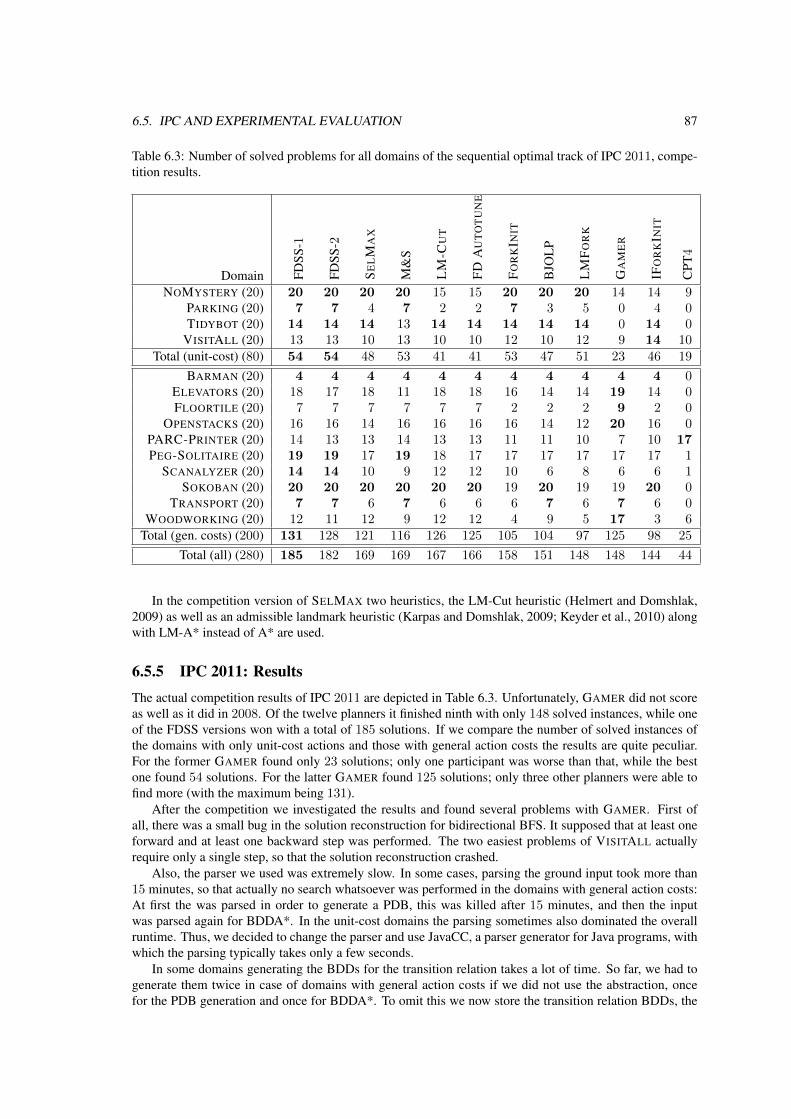
6.5. IPC AND EXPERIMENTAL EVALUATION 87
Table 6.3: Number of solved problems for all domains of the sequential optimal track of IPC 2011, compe-tition results.
Domain FDSS
-1
FDSS
-2
SE
LM
AX
M&
S
LM
-CU
T
FD
AU
TO
TU
NE
FO
RK
INIT
BJO
LP
LM
FO
RK
GA
ME
R
IFO
RK
INIT
CPT
4
NOMYSTERY (20) 20 20 20 20 15 15 20 20 20 14 14 9PARKING (20) 7 7 4 7 2 2 7 3 5 0 4 0TIDYBOT (20) 14 14 14 13 14 14 14 14 14 0 14 0
VISITALL (20) 13 13 10 13 10 10 12 10 12 9 14 10Total (unit-cost) (80) 54 54 48 53 41 41 53 47 51 23 46 19
BARMAN (20) 4 4 4 4 4 4 4 4 4 4 4 0ELEVATORS (20) 18 17 18 11 18 18 16 14 14 19 14 0FLOORTILE (20) 7 7 7 7 7 7 2 2 2 9 2 0
OPENSTACKS (20) 16 16 14 16 16 16 16 14 12 20 16 0PARC-PRINTER (20) 14 13 13 14 13 13 11 11 10 7 10 17PEG-SOLITAIRE (20) 19 19 17 19 18 17 17 17 17 17 17 1
SCANALYZER (20) 14 14 10 9 12 12 10 6 8 6 6 1SOKOBAN (20) 20 20 20 20 20 20 19 20 19 19 20 0
TRANSPORT (20) 7 7 6 7 6 6 6 7 6 7 6 0WOODWORKING (20) 12 11 12 9 12 12 4 9 5 17 3 6
Total (gen. costs) (200) 131 128 121 116 126 125 105 104 97 125 98 25
Total (all) (280) 185 182 169 169 167 166 158 151 148 148 144 44
In the competition version of SELMAX two heuristics, the LM-Cut heuristic (Helmert and Domshlak,2009) as well as an admissible landmark heuristic (Karpas and Domshlak, 2009; Keyder et al., 2010) alongwith LM-A* instead of A* are used.
6.5.5 IPC 2011: ResultsThe actual competition results of IPC 2011 are depicted in Table 6.3. Unfortunately, GAMER did not scoreas well as it did in 2008. Of the twelve planners it finished ninth with only 148 solved instances, while oneof the FDSS versions won with a total of 185 solutions. If we compare the number of solved instances ofthe domains with only unit-cost actions and those with general action costs the results are quite peculiar.For the former GAMER found only 23 solutions; only one participant was worse than that, while the bestone found 54 solutions. For the latter GAMER found 125 solutions; only three other planners were able tofind more (with the maximum being 131).
After the competition we investigated the results and found several problems with GAMER. First ofall, there was a small bug in the solution reconstruction for bidirectional BFS. It supposed that at least oneforward and at least one backward step was performed. The two easiest problems of VISITALL actuallyrequire only a single step, so that the solution reconstruction crashed.
Also, the parser we used was extremely slow. In some cases, parsing the ground input took more than15 minutes, so that actually no search whatsoever was performed in the domains with general action costs:At first the was parsed in order to generate a PDB, this was killed after 15 minutes, and then the inputwas parsed again for BDDA*. In the unit-cost domains the parsing sometimes also dominated the overallruntime. Thus, we decided to change the parser and use JavaCC, a parser generator for Java programs, withwhich the parsing typically takes only a few seconds.
In some domains generating the BDDs for the transition relation takes a lot of time. So far, we had togenerate them twice in case of domains with general action costs if we did not use the abstraction, oncefor the PDB generation and once for BDDA*. To omit this we now store the transition relation BDDs, the

88 CHAPTER 6. CLASSICAL PLANNING
Table 6.4: Number of solved problems for all domains of the sequential optimal track of IPC 2011, ownresults.
M&S M&S M&S GAMER GAMERDomain greedy DFP-gop combined IPC Post-IPC
NOMYSTERY (20) 13 20 20 14 14PARKING (20) 7 0 7 0 0TIDYBOT (20) 13 0 13 0 6
VISITALL (20) 13 11 14 9 11Total (unit-cost) (80) 46 31 54 23 31
BARMAN (20) 4 4 4 4 5ELEVATORS (20) 0 11 11 19 19FLOORTILE (20) 3 7 7 8 9
OPENSTACKS (20) 4 16 16 20 20PARC-PRINTER (20) 11 14 14 7 7PEG-SOLITAIRE (20) 0 19 19 17 17
SCANALYZER (20) 6 10 10 6 9SOKOBAN (20) 1 20 20 19 19
TRANSPORT (20) 6 7 7 7 7WOODWORKING (20) 9 6 9 16 16
Total (gen. costs) (200) 44 114 117 123 128
Total (all) (280) 90 145 171 146 159
BDD for the initial state and that for the goal condition on the hard disk; storing and reading them is oftena lot faster than generating them again from scratch.
In two of the new domains, namely PARKING and TIDYBOT, we found that the first backward step takestoo long, often even more than 30 minutes, so that the decision whether to use bidirectional or unidirectionalBFS could not be finished before the overall time ran out. In these cases, the single images for all theactions were quite fast, but the disjunction took very long. Thus, during the disjunction steps we enteredthe possibility to check whether too much time, in this case 30 seconds, has passed. If it has we stop thedisjunctions and the planner only performs unidirectional BFS (or PDB generation using abstractions). Thisenabled us to find some solutions in TIDYBOT, where in the competition we failed completely. The problemhere is that the goal description allows for too many possibilities, because variables from only very few ofthe SAS+ groups are present.
The FDSS planners seem out of reach for the time being, so that we did not try to compare againstthose, but rather chose one of the planners that finished third, MERGE AND SHRINK. We ran two recent18
versions of MERGE AND SHRINK, one using the greedy bisimulation shrinking strategy (M&S greedy) andone using the DFP-gop shrinking strategy (M&S DFP-gop). The combined results (M&S combined) arethen the number of solutions found within 800 seconds by M&S greedy or withing 1,000 seconds by M&SDFP-gop, just like in the competition setting. We also ran two versions of GAMER, namely the competitionversion (GAMER IPC), and the one with all problems addressed the way we have just described (GAMERPost-IPC). For the experiments we used our own machine (Intel Core i7 920 CPU with 2.67GHz and 24GBRAM) with the same settings concerning timeout (30 minutes) and maximal memory usage (6GB) as inthe competition. The results are depicted in Table 6.4.
On our machine, neither of the two versions of MERGE AND SHRINK took more than 600 seconds forany of the problems. The memory limit of 6GB was what prevented them from finding more solutions.Thus, the competition setting is really reasonable, as it makes the best of both approaches.
From the table we see that the results of the competition version of GAMER have become slightlyworse than on the competition machine, showing that our machine is less powerful than the one used in thecompetition, while those of MERGE AND SHRINK have slightly improved—maybe due to some bugfixesand performance boosts in that planner as well.
18Retrieved on February 22nd 2012 from the FAST DOWNWARD repository at http://hg.fast-downward.org.

6.5. IPC AND EXPERIMENTAL EVALUATION 89
All the small improvements helped mainly in the domains with only unit-cost actions. There we arenow able to find the two trivial solutions in VISITALL, as well as six solutions in TIDYBOT. In the domainswith general action costs the new parser helped us to find three additional solutions in the SCANALYZERdomain.
A last change we tried was running BDDA* in all cases, no matter if we are confronted with generalaction costs or not. Thus, for the domains with unit-cost actions we treated all actions as if they had a costof 1. With this we see another small improvement, one solution in the parking domain. Overall, we arrive at160 solutions in the set of competition problems (32 in the domains with unit-cost actions and 128 in thosewith general action costs). If we ignore the PARC-PRINTER domain, which is special in its way of havingextremely high and very diverse action costs, we are now at the top of all the planners in the domains withgeneral action costs.
Compared with the two versions of MERGE AND SHRINK we can now find the same number of solutionsas the one using the DFP-gop shrinking strategy in case of the unit-cost domains. However, the greedyshrinking strategy (and the combination of both) is still ahead of us.
Maybe a downside of GAMER is that so far it uses only a single heuristic. The results of the last IPCindicate that a portfolio of heuristics often helps, at least in case of explicit-state planners. We see the samein case of MERGE AND SHRINK. Each of the two versions alone are worse than the current version ofGAMER, while the combination brings it ahead by a total of twelve additional solutions.

90 CHAPTER 6. CLASSICAL PLANNING

Chapter 7
Net-Benefit Planning
1. A robot may not injure a human being or,through inaction, allow a human being tocome to harm.
2. A robot must obey the orders given toit by human beings, except where suchorders would conflict with the First Law.
3. A robot must protect its own existence aslong as such protection does not conflictwith the First or Second Laws.
Issac Asimov, The Three Laws of Robotics
In contrast to classical planning described in the previous chapter, in net-benefit planning we are con-cerned with a planning problem that specifies certain soft goals or preferences, i. e., goals that do not nec-essarily need to be achieved. Plans achieving these soft goals are awarded some reward, so that the idea ofoptimal net-benefit planning is to find a plan that maximizes the sum of the rewards for achieving soft goalsminus the total action costs.
Definition 7.1 (Net-Benefit Planning Problem). A net-benefit planning problem is described by a tuplePNB = ⟨V,A, I,G,GS , C,U⟩ with V being the variables that build a state, A a set of actions consisting ofprecondition and effect, i. e., an action a ∈ A is given by a pair ⟨pre, eff ⟩, I an initial state, G a set of goalstates, GS a set of soft goals, C a cost function specifying a certain cost for each action inA, and U a utilityfunction specifying a reward for each of the soft goals GS .
A plan πNB for a net-benefit planning problem is defined in the same way as it is for classical planningas being a sequence of actions transforming the initial state to a goal state (see Definition 6.2), but as wehave soft goals where plans achieving them get additional rewards we need to define a new optimalitycriterion. This is called the plan’s net-benefit.
Definition 7.2 (Net-Benefit of a Plan). Let πNB = (A1, . . . , An) be a plan for a net-benefit planning prob-lem and gS ⊆ GS be the soft goals that are achieved by this plan, i. e., gS ⊆ An (An−1 (. . . A1 (I) . . . )).The plan’s net-benefit is then defined as NB (πNB ) = U (gS) − C (πNB ) with U (gS) :=
g∈gS
U (g)being the total achieved utility (the total reward) and C (πNB ) being the plan’s cost, i. e., the sum of thecosts of all actions within the plan, as defined in Definition 6.3.
Definition 7.3 (Optimal Plan). A plan πNB for a net-benefit planning problem is called optimal, if there isno plan π′
NB with NB (π′NB ) < NB (πNB ).
In the following we will first of all extend the running example to the net-benefit planning setting (Sec-tion 7.1) before we give a brief overview of existing approaches for finding plans for a subset of net-benefitplanning problems, the so-called over-subscription planning problems (Section 7.2). Afterward we present
91

92 CHAPTER 7. NET-BENEFIT PLANNING
p1
p2
p3 p6
p8
p9
p7
p5
p4
p0
2
10
1 4
2
7 5
3
101
312
2 7
7
3 6 1
13gunslinger mib
water water
water
Figure 7.1: The running example in net-benefit planning. The optimal solution is denoted by the thickeredges.
some steps leading to our algorithm for optimally solving net-benefit planning problems, starting with anexisting symbolic branch-and-bound algorithm that we iteratively refine until we come up with our optimalnet-benefit algorithm (Edelkamp and Kissmann, 2009) in Section 7.3. Finally, we will provide the resultsof the international planning competition (IPC) 2008 along with an evaluation of a slight improvement(Section 7.4).
7.1 Running Example in Net-Benefit Planning
For the net-benefit version of the running example of the gunslinger following the man in black through thedesert we decided to add some idea of thirst to the domain. We distinguish four different degrees of thirst(not thirsty, thirsty, very thirsty, and dead). The thirst of the gunslinger increases with each move he takes,so that he can only make two moves and then must drink something or die, hallucinating that he caught theman in black. Because the gunslinger did not expect to enter the desert he does not carry any water, so hemust make use of the water he can find in certain locations of the desert (cf. Figure 7.1).
In order to allow the gunslinger to drink some water we need an additional action:
(:action drink:parameters (?l - location):precondition(and
(position gunslinger ?l) (waterAt ?l)(< (thirst) 3)
):effect(assign (thirst) 0)
)
This reduces the thirst level to no thirst, and can be applied if the gunslinger is at a location where he canfind water and if he has not yet died. The other actions must specify that they can also only applied whenthe thirst is not yet deadly, i. e., (< (thirst) 3) must be part of the precondition, but the move actionsmust increase the thirst, i. e., (increase (thirst) 1) must be added to the effects.
The hallucinating is modeled by use of a new action:

7.1. RUNNING EXAMPLE IN NET-BENEFIT PLANNING 93
(:action hallucinate:parameters (?l - location):precondition(>= (thirst) 3):effect(and
(caughtMIB) (isDead gunslinger))
)
This is the only action that can be applied when the thirst is already deadly.
A plan ending in the gunslinger’s demise is still valid, though he only hallucinated catching the man inblack. This is where the actual net-benefit mechanism comes into play. Instead of just trying to reach a goalstate we specify certain preferences, the soft goals, which should be achieved. Failing one of those will bepenalized. In this case, we define four preferences:
(:goal(and
(caughtMIB)(preference pref_alive (not (isDead gunslinger)))(preference pref_notThirsty (thirsty t0))(preference pref_thirsty (thirsty t1))(preference pref_veryThirsty (thirsty t2))
))
The first one states that the gunslinger should not die, so that he really should have caught the man in black,not just in his hallucination. The next three state that he should be not thirsty at all, only a bit thirsty, orvery thirsty (an even higher degree results in death, as mentioned earlier).
To weight the preferences, we must add them to the metric definition, which in this case looks as follows:
(:metric maximize(- 100
(+(total-cost)(* (is-violated pref_alive) 50)(* (is-violated pref_notThirsty) 25)(* (is-violated pref_thirsty) 20)(* (is-violated pref_veryThirsty) 10)
))
)
What it tells us is that we wish to maximize the outcome of the difference of 100 and the sum of thetotal-cost and the penalty for each violated preference. This way, we actually want to minimize thesum of violations and cost of the plan. The weights for the violations of the four preferences are given inthe multiplication for each of them. Thus, we penalize the failure to stay alive hardest, and we prefer tobe less thirsty. This way, given the action costs as before and the water in locations p2, p4, and p8, in anoptimal solution the gunslinger can safely find a way through the desert to catch the man in black and notdie of thirst on his way there. The optimal solution is as follows, and also displayed in the graph in Figure7.1, where it is denoted by thicker edges.

94 CHAPTER 7. NET-BENEFIT PLANNING
0: (move p0 p2) [1]1: (drink p0) [0]2: (move p2 p3) [4]3: (move p3 p4) [3]4: (drink p4) [0]5: (move p4 p6) [6]6: (move p6 p8) [1]7: (drink p8) [0]8: (move p8 p9) [10]9: (catchMIB p9) [0]
The cost of the actions sums up to 25, while that for the violated preferences sums up to 35, which resultsin a total net-benefit of 40. Another possible plan would be to move from p4 via p7 to p9 and there catchthe man in black, which would reduce the total action cost to 16, but the violation cost would increase to45 because in that case the gunslinger is very thirsty and not just thirsty when he catches the man in black,so that the overall net-benefit in this case would be 39 and thus slightly worse. Another possibility is tojust move between p0 and p2 until the gunslinger dies, which is the case after three moves, resulting in atotal action cost of only 3. But in that case the gunslinger dies, so that we violate all the preferences and theviolation cost thus increases to 105, so that the total net-benefit is −8, which is clearly inferior to the otherresults.
7.2 Related Work in Over-Subscription and Net-Benefit PlanningNet-benefit planning is a comparably new direction so that it has received considerably less interest thanclassical planning, and still does, as we can see from the participants in the international planning competi-tion. In 2008 there were three teams in the optimizing track, in 2011 only one in the optimizing track andone in the satsificing track, so that these tracks were actually canceled.
Net-benefit planning can be seen as the union of classical planning (with general action costs) andover-subscription planning (also called partial satisfaction planning). In contrast to net-benefit planning inover-subscription planning the set of goal states is empty (G = ∅), so that only soft goals are present. Thus,any possible plan is a valid solution for an over-subscription planning problem whose quality is determinedby its net-benefit.
Similar to classical planning, the decision if a plan with a net-benefit that is greater than some positivenumber k can be found is PSPACE-complete (van den Briel et al., 2004).
For the over-subscription planning problem a number of papers have been published during the lastdecade. In the following we will briefly introduce some of those proposing algorithms to find optimalsolutions.
In the work of van den Briel et al. (2004) three methods for solving over-subscription planning problemsare proposed. The first one, which they called OPTIPLAN, is an approach that translates the planningproblem into an integer program. In principle it is an extension of Vossen et al.’s (1999) idea to solveplanning problems by integer programming—but adapted to the over-subscription case. OPTIPLAN findsoptimal plans.
The second one, called ALTALTps , extends ALTALT (Nguyen et al., 2002; Sanchez Nigenda and Kamb-hampati, 2003), a heuristic regression planner. This derives a reachability heuristic from planning graphs.The main extension consists of another approach for heuristically selecting a subset of the soft goals that islikely to be most useful. Using these soft goals as the goal state, a classical planning approach can be usedto solve the resulting planning problem. Nevertheless, if the heuristic chooses bad soft goals, the approachcannot find an optimal plan. To remedy this, ALTALTps needs to create all possible subsets of soft goalsand find an optimal plan for each of these. To ensure optimality it is necessary to use an admissible heuristicduring the search.
The third approach, called SAPAps , extends the forward state-space planner SAPA (Do and Kambham-pati, 2003) in that it does not select a subset of the soft goals before the planning process (as ALTALTps
does) but treats the soft goals as soft constraints, i. e., (as no goal states are present) any possible plan is asolution, but its quality is determined by its net-benefit. SAPAps estimates the g (distance from I) and h

7.3. FINDING AN OPTIMAL NET-BENEFIT PLAN 95
(estimate on the distance to a goal state) values of partial solutions and uses them to guide an A* search. Intheir proposal, SAPAps is not necessarily optimal, but it can be made optimal, if an admissible heuristic isused.
An approach to handle net-benefit planning problems proposed by Keyder and Geffner (2009) is tocompile the soft goals away and use a planner that can handle classical planning input. The idea is totransform each soft goal gS ∈ GS into a classical goal and add two actions, both achieving that goal. Theactions have cost 0 if gS holds in the precondition and cost U (gS) if it does not. An additional actionis required with the precondition being the goal of the net-benefit problem and the effect that some newpredicate end-mode now holds. The preconditions of all actions from the net-benefit problem are extendedby the negation of end-mode, while those for the soft goals take end-mode as a precondition. This way,a plan is actually the plan as it is in the net-benefit problem, followed by the action adding end-mode,followed by a number of actions setting the soft goals, and the cost of that plan corresponds to the negationof the net-benefit of the first part of the plan in the net-benefit specification.
7.3 Finding an Optimal Net-Benefit PlanIn the following, we present our approach to find a plan achieving optimal net-benefit. First of all, weslightly adapt the definition of net-benefit planning and also a plan’s net-benefit (Edelkamp and Kissmann,2009).
Definition 7.4 (Adapted Net-Benefit Planning Problem). An adapted net-benefit planning problem is atuple PNB = ⟨V,A, I,G,PC, Ca, Cc⟩ with V being the variables that build a state, A a set of actionstransforming states into states, I an initial state, G a set of goal states, PC a set of preference constraints,Ca a cost function specifying a certain cost for each action inA, and Cc a cost function specifying a certaincost when failing to achieve one of the constraints.
With this change from soft goals with utilities for achieving them to constraints with costs for failing toachieve them the adaptation of a plan’s net-benefit is straight-forward.
Definition 7.5 (Adapted Net-Benefit of a Plan). Let πNB = (A1, . . . , An) be a plan for an adapted net-benefit planning problem and pc ⊆ PC be the preference constraints that are missed by this plan, i. e., pc ∩An (An−1 (. . . A1 (I) . . . )) = ∅. The plan’s net-benefit is then defined as NB (πNB) = C (pc) + C (πNB)with C (pc) :=
p∈pc Cc (p) being the total cost for missing the constraints and C (πNB) being the cost of
all actions within the plan.
Definition 7.6 (Optimal Plan). A plan πNB for an adapted net-benefit planning problem is called optimal,if there is no plan π′
NB with NB (π′NB) > NB (πNB).
Thus, we switched over from the problem of finding a plan maximizing the difference between goalutility and action costs to one minimizing the total cost, i. e., costs for missing constraints plus action costs.As maximization problems can be transformed to minimization problems and adding a constant offset doesnot change the set of optimal plans, any optimal plan for the adapted net-benefit planning problem is also anoptimal plan for the original net-benefit planning problem. The evaluations for the two views do not match,but as we are interested in an optimal plan and not its evaluation this is not a problem.
According to the costs Cc for each of the preference constraints pc ∈ PC, we can calculate an upperbound on the total violation cost C. As none of the violation costs is negative, the upper bound max v issimply the sum of all violation costs, i. e., we cannot get any worse than violating all constraints. The caseof achieving all of the preference constraints, which equals a total cost of 0, is a lower bound minv . Thanksto these bounds we can safely represent the entire range of possible values (from minv to max v) using⌈log (max v −minv + 1)⌉ BDD variables.
For each preference constraint pc ∈ PC of type (preference pc φpc) we associate a variable vpc , whichdenotes the cost of pc (either Cc (pc) if it is violated or 0 if it is satisfied). We further use Φpc (v) =((vpc = Cc (pc))⇔ ¬φpc)∧ ((vpc = 0)⇔ φpc) for evaluating one constraint in the given state and can usethe formula
pc∈PC Φpc (v) to evaluate all preference constraints in one operation.

96 CHAPTER 7. NET-BENEFIT PLANNING
Algorithm 7.1: Symbolic Branch-and-BoundInput: Adapted Net-Benefit Planning Problem PNB = ⟨V,A, I,G,PC, Ca, Cc⟩.Output: Violation cost optimal plan.
1 U ← max v + 1 // Initial upper bound on total violation cost (can never reach U ).2 bound (v)←
U−1i=0 (v = i) // Bound on total violation cost in form of a BDD.
3 open ← I // Start at initial state I.4 closed ← ⊥ // So far, no state has been expanded.5 loop // Repeat, until plan with minimal total violation cost is found.6 if open = ⊥ or U = 0 then return stored plan // All states expanded or all constraints satisfied.7 goals ← open ∧ G // Determine the goal states in the open list.8 eval (v)← goals ∧
pc∈PC Φpc (v) // Evaluate goal states.
9 metric (v)← eval (v) ∧ bound (v) // Retain only values within bound.10 if metric (v) = ⊥ then // If state with better metric value than currently best one is found. . .11 U ← 0 // Start updating upper bound.12 while (eval (v) ∧ (v = U)) = ⊥ do // While smallest value is = U . . .13 U ← U + 1 // Increase bound U .
14 CalculateAndStorePlan (eval (v) ∧ (v = U)) // Calculate plan with cost of U .15 bound (v)←
U−1i=0 (v = i) // Update bound in form of a BDD according to U .
16 closed ← closed ∨ open // Append states to be expanded to the closed list.17 open ← image (open) ∧ ¬closed // Calculate all new successor states.
While the total action cost in classical planning is a monotonically increasing function, the net-benefitdoes not increase monotonically , so that the first found plan is not necessarily optimal. Thus, we perform asymbolic branch-and-bound search (Jensen et al., 2006). In the following, we will show how to adapt thatalgorithm to finally come up with our net-benefit planning algorithm (Edelkamp and Kissmann, 2009).
7.3.1 Breadth-First Branch-and-Bound
Jensen et al.’s symbolic branch-and-bound algorithm (2006) is outlined in Algorithm 7.1. This ignores anyaction costs but rather returns a plan that is optimal with respect to the achieved total violation cost. Itworks by adapting an upper bound U on the total violation cost, which is initialized to max v +1, so that allpossible results are supported. Furthermore, a BDD representation of the bound is necessary, i. e., a BDDthat represents the disjunction of all possible values ranging from 0 to U −1 (line 2). Following Bartzis andBultan (2006), such a BDD can be constructed efficiently.
Starting at the initial state I the algorithm checks if there are no more unexplored states (open = ⊥)or the upper bound U equals 0 (line 6). In both cases we cannot get any better as in the first case we haveexplored all reachable states and in the second we have found a path that satisfies all preference constraints.If we have calculated some plan to this point we can return it, otherwise we return “no plan”.
If we are not yet done we determine the goal states that are contained in the current BFS layer (line 7).For these we calculate the total violation costs (line 8) and remove any states with an evaluation that is notsmaller than the current bound U (line 9). If the set of these states is not empty, we have found a goal statewith a total violation cost smaller than any found before. To find the best one we search from the bottomup, i. e., we start with a violation cost of 0 and increase it until the conjunction with the evaluation is nolonger false (lines 11 to 13). This results in all the states we have reached in the current BFS layer with theminimal violation cost. For these we can calculate a plan, but as we are not certain that this plan is in factoptimal we only store it internally and continue the search with adapted bounds. This calculation of a planworks just as we presented it for BFS in classical planning (Algorithm 6.2).
To continue, we calculate the successor states of the current layer and remove those that were alreadyexpanded before and stored in the set closed (line 17).

7.3. FINDING AN OPTIMAL NET-BENEFIT PLAN 97
Theorem 7.7 (Optimality of symbolic breadth-first branch-and -bound). The symbolic breadth-first branch-and-bound algorithm finds an optimal plan if we do not consider action costs or the length of the resultingplan, i. e., it finds the shortest plan that produces the minimal total violation cost.
Proof. The algorithm stops when one of two conditions holds: Either the set of unexplored states runsempty or a plan satisfying all constraints has been found.
For the second case the optimality is immediately clear, as we are only concerned with the total violationcost. Due to the expansion in the breadth-first manner we are sure that the first found plan satisfying allconstraints has the shortest length among all the plans satisfying all constraints.
For the first case we need to proof that at some point the set of unexplored states definitely will runempty and that at that point the last stored plan is an optimal one.
The fact that eventually the set of unexplored states runs empty is inherited from BFS, which we performhere. The planning problems contain only a finite number of different states and we perform a BFS withfull duplicate elimination, so that no state is expanded more than once.
Though we do not consider all possible plans, we are still certain that the last generated plan is optimal.This is because we only discard states that are clearly inferior. Either they are discarded because theirviolation cost is greater than the current bound, so that in one of the previous steps a better plan has beenfound, or because in the current iteration at least one state with a smaller violation cost exists.
7.3.2 Cost-First Branch-and-Bound
The problem with net-benefit planning in symbolic search is that the total action cost is not bounded, andthus also the net-benefit is not bounded, so that we cannot construct a BDD for this bound, as we can for thetotal violation cost. To overcome this problem we use a structure similar to the one we used in Dijkstra andA* search, i. e., one that stores all states having the same distance from I in the same bucket (Dial, 1969).Thus, we are able to determine the total action cost immediately by checking the bucket’s index.
In a first step we adapt the previous breadth-first branch-and-bound algorithm (Algorithm 7.1) to workin a cost-first manner (see Algorithm 7.2), though this still ignores the total action cost, i. e., it finds a planthat is optimal with respect to the total violation cost and is the one with smallest total action cost amongall those achieving the minimal total violation cost.
Large parts of this are identical to Algorithm 7.1. Note that we do not use immediate duplicate elimi-nation but a delayed one, i. e., once a bucket is to be expanded, all previously expanded states are removedfrom this. Also, we cannot stop immediately after having found an empty bucket, but only when the lastCmax buckets were empty as well, with Cmax being the highest action cost.
Theorem 7.8 (Optimality of symbolic cost-first branch-and-bound). The symbolic cost-first branch-and-bound algorithm for general action costs C (a) ∈ 0, . . . , Cmax, a ∈ A, finds a cheapest plan among allthose achieving the minimal total violation cost.
Proof. The proof is essentially the same as the one for Theorem 7.7. Here, the algorithm also stops afterthe set of unexplored states runs empty or a plan satisfying all constraints has been found.
In the second case optimality is immediate. Due to the cost-wise approach no other plan satisfying allconstraints can have a smaller total action cost.
In the first case we need to proof that the set of unexplored states runs empty (and that the algorithmwill not stop before this) and that the last stored plan is an optimal one.
Here, the set of unexplored states runs empty as the basic algorithm used is Dijkstra’s algorithm witha closed list, which also expands all reachable states. The algorithm recognizes this by checking the lastCmax buckets. If all these are empty all states have been explored. This is sufficient as the maximal actioncost is Cmax , so that all successors of a bucket openg reside in buckets openg+1 through openg+Cmax
.We do not consider all possible plans, but discard only those that are clearly inferior, i. e., either their
violation cost is at least as high as the best one found so far or in the same iteration another plan of smallerviolation cost has been found.

98 CHAPTER 7. NET-BENEFIT PLANNING
Algorithm 7.2: Symbolic Cost-First Branch-and-BoundInput: Adapted Net-Benefit Planning Problem PNB = ⟨V,A, I,G,PC, Ca, Cc⟩.Output: Violation cost optimal plan.
1 U ← maxv +1 // Initial upper bound on total violation cost (can never reach U ).2 bound (v)←
U−1i=0 (v = i) // Bound on total violation cost in form of a BDD.
3 open0 ← I // Start at initial state I.4 closed ← ⊥ // No state expanded so far.5 g ← 0 // Initial state’s distance is 0.6 loop // Repeat, until plan with minimal total violation cost is found.7 if zero-cost actions present then // If there are any zero-cost actions. . .8 calculate zero-cost fix point for openg // Calculate states reachable using only zero-cost actions.
9 openg ← openg ∧ ¬closed // Remove all duplicate states from previous expansions.10 if
gi=g−Cmax+1 openi = ⊥ or U = 0 then return stored plan // All states expanded or
// all constraints satisfied.11 goals ← openg ∧ G // Determine the goal states in the current bucket.12 eval (v)← goals ∧
pc∈PC Φpc (v) // Evaluate goal states.
13 metric (v)← eval (v) ∧ bound (v) // Retain only values within bound.14 if metric (v) = ⊥ then // If state with better metric value than currently best one is found. . .15 U ← 0 // Start updating upper bound.16 while (eval (v) ∧ (v = U)) = ⊥ do // While smallest value is = U . . .17 U ← U + 1 // Increase bound U .
18 CalculateAndStorePlan (eval (v) ∧ (v = U)) // Calculate plan with cost of U .19 bound (v)←
U−1i=0 (v = i) // Update bound in form of a BDD according to U .
20 for all c ∈ 1, . . . , C do // For all action costs. . .21 openg+c ← openg+c ∨ imagec
openg
// Calculate successor states.
22 closed ← closed ∨ openg // Update set of expanded states.23 g ← g + 1 // Iterate to next g-value.
It might be interesting to note that Algorithm 7.2 essentially behaves the same as Algorithm 7.1, al-though now the exploration is cost-first instead of breadth-first; especially the total violation costs of thefound plans match, as both calculate plans optimal with respect to the same metric, i. e., the total violationcost alone.
Corollary 7.9 (Equivalence of Algorithms 7.1 and 7.2). The costs of the plans found by both algorithmsmatch.
7.3.3 Net-Benefit Planning AlgorithmUsing the additional information of the stored buckets we can now propose an algorithm that calculates aplan achieving optimal net-benefit (cf. Algorithm 7.3), so that it considers not only the total violation costbut also the total action cost and finds a plan minimizing the sum of both (Edelkamp and Kissmann, 2009).For this we need a second bound, V , on the net-benefit, which is decreased with each plan we find.
Instead of updating the BDD representing the bound on the violation costs only when a plan has beenfound, we update it before each step (line 11). With this we make sure that only plans that have a violationcost smaller than the current optimum U as well as a net-benefit (which is the violation cost plus g) smallerthan the current optimum V .
Theorem 7.10 (Optimality of the symbolic net-benefit planning algorithm). The symbolic net-benefit plan-ning algorithm finds a plan achieving optimal net-benefit for general action costs C (a) ∈ 0, . . . , Cmax,a ∈ A.

7.3. FINDING AN OPTIMAL NET-BENEFIT PLAN 99
Algorithm 7.3: Symbolic Net-Benefit Planning AlgorithmInput: Adapted Net-Benefit Planning Problem PNB = ⟨V,A, I,G,PC, Ca, Cc⟩.Output: Net-benefit optimal plan.
1 U ← maxv +1 // Initial upper bound on total violation cost (can never reach U ).2 V ←∞ // Initial upper bound on net-benefit.3 open0 ← I // Start at initial state I.4 closed ← ⊥ // No state expanded so far.5 g ← 0 // Initial state’s distance is 0.6 loop // Repeat, until plan achieving optimal net-benefit is found.7 if zero-cost actions present then // If there are any zero-cost actions. . .8 calculate zero-cost fix point for openg // Calculate states reachable using only zero-cost actions.
9 openg ← openg ∧ ¬closed // Remove all duplicate states from previous expansions.10 if
gi=g−Cmax+1 openi = ⊥ or U = 0 or V ≤ g then return stored plan // All states expanded
// or all constraints satisfied or bound on net-benefit greater than distance to I.11 bound (v)←
minU−1,V−gi=0 (v = i) // Update bound in form of BDD according to U , V and g.
12 goals ← openg ∧ G // Determine the goal states in the current bucket.13 eval (v)← goals ∧
pc∈PC Φpc (v) // Evaluate goal states.
14 metric (v)← eval (v) ∧ bound (v) // Retain only values within bound.15 if metric (v) = ⊥ then // If state with better net-benefit than currently best one is found. . .16 U ← 0 // Start updating bound on total violation cost.17 while (eval (v) ∧ (v = U)) = ⊥ do // While smallest value is = U . . .18 U ← U + 1 // Increase bound U .
19 V ← U + g // Update bound on net-benefit.20 CalculateAndStorePlan (eval (v) ∧ (v = U)) // Calculate plan with violation cost of U .
21 for all c ∈ 1, . . . , C do // For all action costs. . .22 openg+c ← openg+c ∨ imagec
openg
// Calculate successor states.
23 closed ← closed ∨ openg // Update set of expanded states.24 g ← g + 1 // Iterate to next g-value.
Proof. Again we need to proof that the algorithm stops once all reachable states have been considered orwhen the best plan found so far cannot be improved. Furthermore, we need to proof that the last stored planis optimal.
Here, in the worst case the algorithm again considers all reachable states. If that happens, the open listruns empty, which is found out by looking at the last Cmax buckets. This suffices as the action costs cannotbe larger than Cmax , so that once Cmax adjacent buckets are empty all states have been considered.
If not all states are considered, the algorithm nevertheless stops once all constraints are satisfied (U = 0),in which case we surely got the optimal result due to the cost-wise expansion, or when the total action costhas reached the smallest total net-benefit found so far (V ≤ g). In this case we would need a negativeviolation cost to come up with a net-benefit smaller than V , which is impossible, as all violation costs areassumed to be non-negative.
What remains is proving that the last stored plan is optimal. In each iteration we only consider thosegoal states whose violation cost is smaller than U and also at most as large as V − g. The second bound isnecessary to discard those states that achieve a better violation cost but still cannot beat the currently bestnet-benefit. Thus, we discard only those states clearly inferior; all others are considered, so that at any timethe last stored plan is the best one we can achieve with the given total action cost.

100 CHAPTER 7. NET-BENEFIT PLANNING
7.4 Experimental EvaluationWe implemented the symbolic net-benefit algorithm in another version of our planner GAMER. This versionis implemented in C++ and uses the BDD package BuDDy19 to handle the BDDs. With it we participatedin the optimal net-benefit track of the International Planning Competition (IPC) 2008 and won that track aswell.
The setting is similar to the one used in the sequential-optimal track (see Section 6.5). The plannerswere also limited to 2GB of main memory and 30 minutes for each problem. Each of the six domains(CREW PLANNING, ELEVATORS, OPENSTACKS, PEG-SOLITAIRE, TRANSPORT, and WOODWORKING)contain 30 problem instances. For many domains several formulations were given and the results of the onea planner performed best in chosen for the comparison.
The comparison was also based solely on the number of solved problems. If a planner found a sub-optimal solution it achieved 0 points for the entire domain. Otherwise, the number of solved instances foreach domain was counted and summed up to build the final score.
The net-benefit track was considerably less popular, so that only three planners participated in 2008. InIPC 2011 two preference planning tracks (which were supposed to be similar to the net-benefit planningtrack of IPC 2008) were announced, but were canceled because in the optimizing track as well as thesatisficing track only one planner wanted to participate.
In the following, we will briefly outline the two competing planners of IPC 2008 (Section 7.4.1). Then,we will show the results achieved during the competition (Section 7.4.2) and finally discuss which of theimprovements proposed Section 6.4 can be transfered to the net-benefit planner as well and compare themost recent version of GAMER with the competition version on a state-of-the-art machine (Section 7.4.3).
7.4.1 IPC 2008: Participating PlannersIn the following we provide short descriptions of the two competitors, HSP∗p and MIPS XXL.
HSP∗p
Haslum’s HSP∗p (2008) performs a simple translation of the net-benefit problems to classical planning prob-lems. It enumerates the set of possible soft goals and finds optimal plans for each. For this it uses regres-sion, IDA* and a variant of the additive h2 heuristic (Haslum and Geffner, 2000). When it is done the planachieving the best net-benefit can be extracted.
This enumeration of the soft goals is also what prevented it from finding any plans in PEG-SOLITAIRE.Even in the most simple problem there are already 33 soft goals, resulting in 233 = 8,589,934,592 sets,which of course cannot all be solved in the short 30 minute time slot.
MIPS XXL
Similar to the sequential-optimal version, MIPS XXL (Edelkamp and Jabbar, 2008) performs externalsearch. In this case, it is actually very similar to the symbolic algorithm, only that it uses files on an externalstorage instead of buckets of BDDs in main memory.
7.4.2 IPC 2008: ResultsThe competition’s results are publicly available on the competition’s website20 and are also given in Table7.1. As we can see, our planner GAMER clearly outperformed the two competing systems MIPS XXL andHSP∗p, though the latter mainly failed because it was not able to solve any of the problems of the PEG-SOLITAIRE domain, as we have mentioned above.
We found that there was a small bug in the implementation of GAMER only recently, which preventedit from finding four simple solutions in the CREW PLANNING domain and two just as simple solutions in
19http://buddy.sourceforge.net20http://ipc.informatik.uni-freiburg.de/Results

7.4. EXPERIMENTAL EVALUATION 101
Table 7.1: Numbers of solved problems for all domains of the optimal net-benefit track of IPC 2008,competition results.
Problem GAMER HSP∗p MIPS XXLCREW PLANNING (30) 4 16 8
ELEVATORS (30) 11 5 4OPENSTACKS (30) 7 5 2
PEG-SOLITAIRE (30) 24 0 23TRANSPORT (30) 12 12 9
WOODWORKING (30) 13 11 9
Total (180) 71 49 55
the PEG-SOLITAIRE domain, all of which can be solved within a few seconds, so that GAMER’s winningmargin increases even further.
7.4.3 Improvements of GAMER
In Section 6.4 we proposed four improvements for our classical planner, i. e., using a map instead of the(g, h)-matrix to handle large action costs, reordering of the variables, an incremental abstraction calculation,and an automatic choice for the amount of backward search (Kissmann and Edelkamp, 2011).
Of these four improvements the last two are not applicable in this algorithm, as it operates strictly inforward direction, so that no abstraction is necessary and no backward search is performed.
We did not yet implement the priority queue as a map instead of a vector for two reasons. The firstis simply that all action costs of the entire test collection are small enough not to cause any problems, thesecond is that we use a one-dimensional vector for storing the layers according to their distance g to theinitial state. Thus, the action costs need to be a lot larger than in classical planning in order for this structureto exceed the available memory.
Thus, all that remains is the implementation of a reordering of the variables, which is the most effectiveof all the improvements in our classical planner. Nevertheless, in the net-benefit planner this reorderingbrings some more problems. While in classical planning we only have groups of binary facts, here we alsohave the preference constraints, which are modeled by BDD variables. Furthermore, the net-benefit plannersupports some numerical variables, which are included into the BDD structure as well. The problem withthese two is that they are not part of the causal graph we construct. Thus, we reorder only the propositionalvariables.
As we cannot evaluate the preference constraint variables, we decided to distribute them equally beforeand after the propositional variables, hoping that the mean distance might decrease. Additionally, we de-cided to implement two versions, one (GAMER r
a) that performs reordering in any case and one (GAMER r¬n)
that performs it only in domains without numerical variables, as it might have a negative effect in such do-mains.
We evaluated these two versions along with the original version of GAMER on our machine, whichcontains an Intel i7 920 CPU with 2.67GHz and 24GB RAM, using a timeout of 30 minutes, but no limiton the usable main memory.
In Table 7.2 we see that using the reordering we can solve some more problems of the OPENSTACKSdomain, while for the other domains there is no change in the number of solved problems. In the classicalplanner the improvement concerning the OPENSTACKS domain was also biggest, but there the numberof solved instances in the WOODWORKING domain also increased a lot, which is not the case for thenet-benefit planner. While the specification of OPENSTACKS is available in several versions, one usingnumerical variables, others not, that for WOODWORKING is only available using numerical variables. Itseems that this is what prevents us from improving over the competition results in that domain.
Comparing the runtimes of the algorithms (cf. Figure 7.2) we see only three domains where the reorder-ing has a measurable impact. In two of these, namely OPENSTACKS (Figure 7.2d) and PEG-SOLITAIRE(Figure 7.2e), the runtime decreases by a factor of up to 16.5 and 2.6, respectively. The last one, ELEVA-TORS is an example of a domain where the reordering is counter-productive, as there the runtime increases

102 CHAPTER 7. NET-BENEFIT PLANNING
Table 7.2: Numbers of solved problems for all domains of the optimal net-benefit track of IPC 2008, ownresults.
Problem GAMER GAMER ra GAMER r
¬n
CREW PLANNING (30) 8 8 8ELEVATORS (30) 19 19 19
OPENSTACKS (30) 7 12 12PEG-SOLITAIRE (30) 30 30 30
TRANSPORT (30) 15 15 15WOODWORKING (30) 16 16 16
Total (180) 95 100 100
by a factor of up to 1.5 in the formulation containing numerical variables (Figure 7.2b) and up to 1.8 in theSTRIPS formulation (Figure 7.2c).
From these results and those for the classical planner it seems that we must extend the causal graph weuse for the reordering, so that it can also capture the numerical variables and the preference constraints.If we cannot properly reorder the entire set of variables we often will not improve much over the originalordering.

7.4. EXPERIMENTAL EVALUATION 103
0
200
400
600
800
1000
1200
1400
1600
1800
5 10 15 20 25 30
Run
time
[s]
Problem
GAMERGAMER r
aGAMER r
¬n
(a) CREW PLANNING (numeric).
0
200
400
600
800
1000
1200
1400
1600
1800
5 10 15 20 25 30
Run
time
[s]
Problem
GAMERGAMER r
aGAMER r
¬n
(b) ELEVATORS (numeric).
0
200
400
600
800
1000
1200
1400
1600
1800
5 10 15 20 25 30
Run
time
[s]
Problem
GAMERGAMER r
aGAMER r
¬n
(c) ELEVATORS (STRIPS).
0
200
400
600
800
1000
1200
1400
1600
1800
5 10 15 20 25 30
Run
time
[s]
Problem
GAMERGAMER r
aGAMER r
¬n
(d) OPENSTACKS (STRIPS).
0
200
400
600
800
1000
1200
1400
1600
1800
5 10 15 20 25 30
Run
time
[s]
Problem
GAMERGAMER r
aGAMER r
¬n
(e) PEG-SOLITAIRE (STRIPS).
0
200
400
600
800
1000
1200
1400
1600
1800
5 10 15 20 25 30
Run
time
[s]
Problem
GAMERGAMER r
aGAMER r
¬n
(f) TRANSPORT (numeric).
0
200
400
600
800
1000
1200
1400
1600
1800
5 10 15 20 25 30
Run
time
[s]
Problem
GAMERGAMER r
aGAMER r
¬n
(g) WOODWORKING (numeric).
Figure 7.2: Runtime results for all domains of the optimal net-benefit track of IPC 2008 on our own ma-chine. The caption denotes if it contains numerical variables (numeric) or not (STRIPS).

104 CHAPTER 7. NET-BENEFIT PLANNING

Part III
General Game Playing
105


Chapter 8
Introduction to General Game Playing
All work and no play makes Jack a dull boy.
Proverb
Game playing has been an important topic in research for a long time. On the one hand the resultsconcerning equilibria by Nash, Jr. (1951) are still used especially in economics but also in several otherdomains. On the other hand, in AI games provide a good testbed as they often are not trivial and algorithmshelping to speed up search for solutions or at least good moves can often be applied in other topics of AI(Russell and Norvig, 2010).
The first notable successes occurred in the 1990s, when several machines were able to defeat reigningworld champions in their corresponding games. Of course, there were earlier success stories, such as thesolving of CONNECT FOUR (Allen, 1989; Allis, 1988) or the NIM game, but important as they might bein the AI community, the defeat of a human by a machine in a real championship match in much morecomplicated games was what received much larger public interest.
The first one of these successes was the victory of the AMERICAN CHECKERS program CHINOOK(Schaeffer et al., 1992; Schaeffer, 1997) against the supposedly best human AMERICAN CHECKERS playerof all time, Marion Tinsley. The first match in 1990 in the newly created Man versus Machine WorldChampionship was won by Tinsley by a final outcome of four against two victories, with a total of 33draws. Thus, Tinsley was defeated in two of the games but remained the world champion.
In 1994, a rematch was performed, but after six draws Tinsley had to retire, as he suffered from cancer.In the wake of this CHINOOK was declared world champion, though it had never actually defeated the bestplayer in a complete match.
In an additional match in 1995 CHINOOK defeated its title against Don Lafferty, the number two afterTinsley, in a match with one victory and 31 draws. Afterward, CHINOOK’s main developer, JonathanSchaeffer, decided to retire CHINOOK from active play and concentrated on solving the game.
Another important victory for AI research is due to the CHESS player DEEP BLUE (Campbell et al.,2002). In a first match in February 1996 it defeated the reigning world champion Garry Kasparov in thefirst game, but lost three of the following five games; the remaining two resulted in a draw, so that the finaloutcome was 4 – 2 for Kasparov (with wins counting as one point and draws as 0.5 points).
In a rematch in May 1997 DEEP BLUE was able to defeat Kasparov with a final outcome of 3.5 – 2.5and thus became the first machine to beat a human world champion in the game of CHESS.
In the same year, Michael Buro’s LOGISTELLO (Buro, 1997) was able to beat the world champion inthe game of OTHELLO, Takeshi Murakami, in a match with a final outcome of six against zero wins.
All these victories are remarkable successes, but a question one might ask is: Are the players reallyintelligent? Of course, the computers are used and necessarily needed to perform that good, nevertheless itis the programmer that inserts lots of domain specific knowledge such as expert knowledge and specializedheuristics into the players to enable them to perform well in the one game they were designed for. Due tothe restriction to just one game the computers, are not able to play any other games. Thus, one might arguethat the intelligence really comes from the programmers, not the programs.
107

108 CHAPTER 8. INTRODUCTION TO GENERAL GAME PLAYING
One approach to overcome this problem is the idea of general game playing (GGP) (Genesereth et al.,2005). In this, the actual games to be played are unknown to the programmers; they only know the languagefor the description of possible games. The program must then read such a description and evaluate it in orderto play the game. Furthermore, it must find sensible moves on its own to succeed. Thus, the programmercannot insert any domain specific knowledge.
This setting is very similar to action planning. While in classical planning we are concerned withproblems for only one player—the planner—that tries to reach one goal, in general game playing we areconcerned with one or more players performing their moves concurrently, each with its own goals thatmight contradict those of the other players. Also, we typically have goals where a player achieves differentrewards, so that here we prefer to speak of terminal states instead of goal states. Such a rewarding ofachieving certain goals is actually similar to over-subscription planning. Another tight relationship we canidentify is to adversarial or non-deterministic planning, where the environment might be interpreted as anopponent, so that we actually can use approaches for two-player games to find solutions in that setting(Bercher and Mattmuller, 2008; Kissmann and Edelkamp, 2009b).
An early approach in the direction of GGP was Barney Pell’s METAGAME (Pell, 1992a). The idea ofMETAGAME is to have a game generator, which produces new games according to a pre-defined class ofgames. The best way to compare different programs is to run a tournament and let the programs play againsteach other—typically, the best (i. e., most intelligent) program should be able to win.
The interest in GGP has increased in recent years, mainly due to a new project initiated by the gamesgroup of Stanford University21. It became especially popular with the launch of an annual competition(Genesereth et al., 2005), which is held since 2005, originally only in the context of the national AAAIconference, nowadays also at the International Joint Conference on Artificial Intelligence (IJCAI).
The language that is used for these competitions is the Game Description Language GDL (Love et al.,2006), which is an extension of Datalog and thus a logic based language. In GDL it is possible to definesingle- or multiplayer games that are deterministic, discrete, and finite and where all players have fullinformation of the game rules, the current state and the moves performed. Thus, in contrast to Pell’s gameclasses, e. g., the symmetric CHESS-like games (Pell, 1992b) he proposed in the context of METAGAME,this approach is more general, though still quite limited.
Two of the most limiting factors, i. e., the restrictions that the games must be deterministic and that theplayers must have full information, have recently been lifted by Thielscher’s (2010) proposal of GDL-II(for GDL with Incomplete Information). To achieve this he introduced a special role, random, which hasno goals and always chooses a move randomly, and by the introduction of a new relation symbol, sees,which determines what a player actually sees of the current state. So far, research has mainly focused onthe older GDL specification, though with GDL-II clearly more interesting games can be described. In thecontext of the international competition at AAAI or IJCAI no GDL-II track has been performed so far; theonly international competition that did this was the first German Open in GGP we organized in the contextof the 34th German Conference on Artificial Intelligence (KI) in 2011.22
In the remainder of this chapter we will introduce the Game Description Language GDL (Section 8.1),point out the main differences to the Planning Domain Definition Language PDDL (McDermott, 1998)(Section 8.2), which is the default language for describing action planning problems, and provide somemore details in a short comparison to action planning (Section 8.3).
In Chapter 9 we will describe a way to instantiate GDL, i. e., to get rid of the variables in order to inferknowledge faster and to be able to use BDDs in the general game playing domain. Then, in Chapter 10 wewill propose a few algorithms (using symbolic search) to actually solve general games, while Chapter 11 isconcerned with playing the games and describing our approach to implement a general game player.
8.1 The Game Description Language GDLIn recent years, the Game Description Language GDL (Love et al., 2006), the language used at the annualAAAI or IJCAI GGP competition (Genesereth et al., 2005), has become the language of choice for thedescription of general games. In this work we are only concerned with the original GDL, so that the
21http://games.stanford.edu22http://fai.cs.uni-saarland.de/kissmann/ggp/go-ggp

8.1. THE GAME DESCRIPTION LANGUAGE GDL 109
games are restricted to be deterministic, discrete and finite games of full information, but allow for single-and multiplayer settings. Nowadays, some extensions have been proposed, e. g., the Market SpecificationLanguage (MDL) (Thielscher and Zhang, 2009) that inserts support for incomplete information and is usedin the Trading Agent Competition TAC, or GDL-II (Thielscher, 2010), which inserts non-determinism andincomplete information.
8.1.1 The Syntax of GDL
Though a detailed description of GDL’s syntax can be found in the report by Love et al. (2006), in this sec-tion we repeat several of those definitions in the following, as we need some idea of how a game descriptionis organized when instantiating it (Chapter 9).
Definition 8.1 (Vocabulary). The vocabulary of GDL consists of sets of relation symbols with correspondingarity, function symbols with corresponding arity and object constants. Furthermore, it contains variables,which are denoted by the prefix ? in GDL.
Definition 8.2 (Term). A GDL term is either a variable, an object constant or a function symbol of somearity t applied to t terms.
This nesting of function symbols is explicitly allowed, though it is restricted due to the requirementof the games to be finite. Nevertheless, it is used only in a small number of available games. Except forour player (cf. Chapter 11) we so far ignore games that make use of this; especially the instantiator cannothandle nested terms.
Definition 8.3 (Atomic Sentence, Literal, Expression, and Ground Expression). An atomic sentence (oratom for short) is a relation symbol of some arity t applied to t terms. A literal is an atomic sentence orthe negation of an atomic sentence. Terms and literals are also called expressions. Such an expression iscalled ground iff it does not contain any variables.
Definition 8.4 (Rule and Fact). A GDL rule is an implication of the form B ⇒ h (though typically writtenthe other way around, i. e., h⇐ B). The body B of the implication is a conjunction b1 ∧ · · · ∧ bn of eitherliterals or disjunctions of literals. The head h is an atomic sentence. A rule with only a head and no bodyis called a fact.
Note that in a more recent specification of GDL the body of a rule may no longer contain disjunctions,so that we are actually confronted with Horn rules, and the safety property must hold.
Definition 8.5 (Horn Rule). A GDL rule is called Horn if its body is a conjunction of literals.
Definition 8.6 (Safety Property). For a Horn rule the safety property holds if any variable appearing in thehead or in any negative literal also appears in a positive literal in the body.
We stick to the older notion because there are still many games that use disjunctions. Also, in ourexperience game descriptions using disjunctions tend to be shorter and easier to understand by humans,though that is of no concern in the development of a GGP agent.
In GDL, all rules are implicitly connected by disjunction, so that it is possible to split rules containingdisjunctions into a number of Horn rule. Thus, we can see the older notion with disjunctions modeledexplicitly and the newer one without those as equivalent in terms of expressiveness.
Lemma 8.7 (Splitting of rules). Any rule according to Definition 8.4 can be converted to a number Hornrules.
Proof idea. The idea is to calculate the disjunctive normal form (DNF) by applying the distributive propertyand to split a rule if its base operator is a disjunction, i. e., a rule in DNF of the form h⇐ b′1∨ · · ·∨ b′m witheach b′i being either a literal or a conjunction of literals can be split to m rules h⇐ b′1, . . . , h⇐ b′m.

110 CHAPTER 8. INTRODUCTION TO GENERAL GAME PLAYING
Note that for a rule to be a valid GDL rule, after the splitting the safety property must hold in all resultingHorn rules.
In GDL negation is treated as negation-as-failure. To avoid any problems arising from this treatment therules must be stratified. Stratification of a set of rules means that some relation r may never be dependenton the negation of r. Thus, the stratification is defined based on a dependency graph.
Definition 8.8 (Dependency Graph). For a set of GDL rules a dependency graph can be constructed. Itsnodes are the relation symbols in the vocabulary and it contains an edge from r2 to r1 if there is a rule withhead r1 and with r2 in the body. If r2 is a negative literal the edge is labeled with ¬.
Definition 8.9 (Stratified Rules). A set of GDL rules is stratified iff the corresponding dependency graphdoes not contain any cycles that include an edge labeled with ¬.
Stratification alone is not enough. In case we are confronted with recursive rules we must make surethat we cannot run into cycles. Thus, each GDL rule must also obey the recursion restriction.
Definition 8.10 (Recursion Restriction). Given a set of GDL rules containing a rule of the form
p (a1, . . . , apn)⇐ b1 ∧ · · · ∧ bk (v1, . . . , vkn
) ∧ · · · ∧ bn
where bk is in a cycle with p in the dependency graph representation. Then the recursion restriction holdsif for all j ∈ 1, . . . , kn it holds that vj is a constant, or vj ∈ a1, . . . , apn
, or ∃i ∈ 1, . . . , n . bi =r (. . . , vj , . . . ) for some relation symbol r that does not share a cycle with p in the dependency graphrepresentation.
The semantics of GDL is based on first-order logic semantics (with negation being treated as negation-as-failure. Thus, we will skip the details and refer the reader to the original GDL specification (Love et al.,2006).
8.1.2 Structure of a General GameIn contrast to PDDL in GDL we do not have two descriptions for the domain and a certain instance ofthat domain, but rather both are done together in one description. It consists of the specification of severalaspects of the game, which we will describe in more detail in the following. To make things clearer, we willexplain the different concepts along our running example of the man in black running through the desertfollowed by the gunslinger.
While in the planning formulations we restricted ourselves to a static man in black, which the gunslingerhad to reach on a path as short as possible, here we can finally allow the man in black to move as well. Thus,in this formulation the gunslinger starts at position p0 and the man in black (mib) has only a small headstart at position p3 (cf. Figure 8.1). The game would be awfully easy if both were equally fast, so that wedecided to allow the gunslinger to move a distance of two positions in one step, while the man in black canonly move as far as an immediately adjacent position. The game would still not be any challenge whatsoeverif the two players moved alternatingly, so that instead they move simultaneously and the gunslinger can onlywin if he reaches the same position as the man in black unless it is the end of the desert at position p9 wherethe man in black is able to escape and thus win the game. To keep the game finite we use a step counter, sothat the game ends after ten steps if neither the gunslinger succeeds in capturing the man in black nor theman in black succeeds in escaping.
A part of the game’s description is given in Figure 8.2; the full description can be found in Appendix A.
Definition 8.11 (General Game). A general game is a tuple G = ⟨P,L,N ,A, I, T ,R⟩ with P being theset of available players or roles, L the set of legal rules, N the set of next rules, A the set of rules foradditional relations, which we call axioms, I the initial state, T the set of terminal states, andR the set ofreward rules.
In GDL, which uses the same notation as the knowledge interchange format KIF (Genesereth and Fikes,1992), all predicates and formulas are in prefix notation and variables are denoted by the prefix ?. Severalrelations are predefined in GDL. In the following we will outline the meanings of these relations and showhow they are implemented in our example game.

8.1. THE GAME DESCRIPTION LANGUAGE GDL 111
p1
p2
p3 p6
p8
p9
p7
p5
p4
p0gunslinger mib
(a) Initial state.
p1
p2
p3 p6
p8
p9
p7
p5
p4
p0
gunslinger
mib
(b) Terminal state won by the mib.
Figure 8.1: GDL version of the running example.
(role gunslinger) (role mib)
(init (position gunslinger p0))(init (position mib p3))(init (step 0))
(<= (legal gunslinger (move ?l1 ?l3))(true (position gunslinger ?l1))(adjacent ?l1 ?l2) (adjacent ?l2 ?l3) (distinct ?l1 ?l3))
(<= (legal mib (move ?l1 ?l2))(true (position mib ?l1)) (adjacent ?l1 ?l2))
(<= (next (position ?p ?l2))(does ?p (move ?l1 ?l2)))
(<= (next (step ?s2))(true (step ?s1)) (succ ?s1 ?s2))
(<= terminal caughtMIB)(<= terminal escapedMIB)(<= terminal (true (step 10)))
(<= (goal mib 100) escapedMIB)(<= (goal mib 10)
(true (step 10)) (not caughtMIB) (not escapedMIB))(<= (goal mib 0) caughtMIB)
(succ 0 1) ... (succ 9 10)(adjacent p0 p1) ... (adjacent p8 p9)(adjacent p1 p0) ... (adjacent p9 p8)
(<= caughtMIB(true (position gunslinger ?l)) (true (position mib ?l))(not escapedMIB))
(<= escapedMIB (true (position mib p9)))
Figure 8.2: Part of the GDL description of the running example.
Roles To specify the roles of the different players, the unary relation role is used. The only argumentis a player’s name within the game description. All roles must be defined at the start of the gameand the set of players may never change in the course of one game. According to the specification,

112 CHAPTER 8. INTRODUCTION TO GENERAL GAME PLAYING
a role relation may only appear as a fact, though in practice lots of games use this keyword withinthe bodies of other rules to simplify the description.
In the running example, we have two players, gunslinger and mib.
Fluents In GDL a state is described by functions for which the relation true holds in that state. These arecalled fluents.
Initial State The initial state is specified by the unary relation init. It might either be a head of a rule ora fact. The argument of init is a function and all possible instantiations of this argument denote theset of fluents true in the initial state. Any fluent that is not a possible instantiation of the argumentdoes not hold initially.
In the example the initial state consists of two position fluents, specifying the position of thegunslinger and of the man in black at the start of the game. Additionally, the step counter isinitially set to 0. Note that we could have chosen any other object constant, as GDL does not knowthe concept of numbers.
Inequality In several cases it is important to know that some parameters must differ. For those cases thebinary relation distinct is used. As this is an implicit negation, if any of the two arguments isa variable due to the safety property (cf. Definition 8.6) that variable must also appear in a positiveliteral within the same rule.
Legal Moves In any reachable non-terminal state all players must choose a move. GDL specifies whatmoves are possible in which state. The rule’s head is the binary legal relation. The first argumentof this is the player’s name, the second the move that the player can perform.
By default, GDL allows only the description of simultaneous-move games. To make a game turn-taking (or, more generally, non-simultaneous), such as CONNECT FOUR, CHESS and many others,a noop (for no operation) move must be specified. This is the only move that can be chosen bythe player who is not the active one. In order to make the example game turn-taking, we need anadditional fluent, control. This specifies which player is currently the active one and may performa move. A legal rule in the turn-taking setting then looks like this:
(<= (legal mib (move ?l1 ?l2))(true (control mib))(true (position mib ?l1)) (adjacent ?l1 ?l2))
Chosen Moves To denote which moves the players have chosen the does relation is used. Similar to thelegal relation it is a binary relation with the first argument denoting the player who has chosen themove specified in the second argument. This relation appears only in the body of rules.
Successor States To determine the successor state once all players have chosen a move the unary nextrelation is used. Its single argument is a function that denotes a fluent true in the successor state. Thisrelation may only appear as the head of a rule.
Note that in GDL the frame is modeled explicitly, i. e., any fluent that is not the argument of thehead of a satisfied next rule is supposed to be false in the successor state. Due to this the gamedescriptions tend to be a bit more lengthy than those of PDDL, where the frame is modeled implicitly,so that only those facts that change are given in the effects of an action.
In the example game both players move simultaneously and the first next rule updates their posi-tions. The step counter is increased by the second next rule. These are the only next rules weneed in this game; the frame is no problem here. If the game was turn-taking things would look a bitdifferent. In that case, we would need to store the position of the player whose turn it is to wait, forexample:
(<= (next (position ?p ?l))(true (position ?p ?l)) (not (true (control ?p))))

8.2. DIFFERENCES BETWEEN GDL AND PDDL 113
Terminal States Once a terminal state is reached the game ends and no more moves are performed by anyof the players. To determine when a terminal state is reached the terminal rules are used. Onceone of these is satisfied the game ends.
The example game ends in one of three cases. Either if the man in black is caught, or the man inblack has escaped or the step counter has reached the value of 10.
Rewards To generate the outcome of a game, i. e., to determine the rewards for all the players, the binarygoal relation is used with the first argument being the player for whom this relation is relevant andthe second one the reward that player will get. The rewards are integral and range from 0 to 100, withhigher rewards being better.
In the example game the winner gets 100 points and the loser 0, i. e., if the man in black can escapehe has won; if he is caught before escaping the gunslinger has won. In case no one has won and thestep counter has ended the game both players get 10 points.
Additional Relations All additional relations, the axioms, can appear anywhere, i. e., they can be part ofthe body of a rule, the head of a rule or also a fact. They are similar to the derived predicates fromPDDL. In principle, this is a way to keep the game description shorter (and thus also more readable),as they can be removed by replacing each appearance of a relation by the body of a correspondingrule.
Examples for this concept in the example game are the relations succ, adjacent, caughtMIB,and escapedMIB, denoting a successor relation for the step counter, the adjacency of the positions,whether the man in black has been caught, and whether the man in black has escaped, respectively.
GDL constrains the description further than just to deterministic, discrete and finite games of full in-formation following the definitions of Section 8.1.1. In order to produce well-formed games, which wetypically expect in a competition setting, the description must satisfy three additional conditions. Onceagain, these definitions are from the original GDL specification (Love et al., 2006).
Definition 8.12 (Termination). A general game terminates if all (infinite) sequences of legal moves from theinitial state reach a terminal state after a finite number of steps.
Definition 8.13 (Playability). A general game is playable iff each player has at least one legal move inevery reachable state that is not terminal.
Definition 8.14 (Winnability). A general game is strongly winnable iff for one player there is a sequenceof moves of that player that leads to a terminal state where that player receives the maximal reward of100 points, i. e., if the player can find a sequence of moves that ensure victory, no matter what moves theopponents perform.
A general game is weakly winnable iff for every player there is a sequence of joint moves of all playersthat leads to a terminal state where that player receives the maximal reward of 100 points, i. e., if it ispossible that the player can achieve the maximal reward if the other players help it to achieve this goal.
Note that a single-player game that is weakly winnable is also strongly winnable.
Definition 8.15 (Well-Formed Game). A general game is well-formed if it terminates, is playable and isweakly winnable.
8.2 Differences between GDL and PDDLApart from the ability to describe multiplayer games instead of just single-agent planning problems the twoinput languages PDDL and GDL differ in several other points as well.
• In GDL, no list of all relation symbols or object constants is provided. They can only be determinedby scanning the complete game description.

114 CHAPTER 8. INTRODUCTION TO GENERAL GAME PLAYING
• GDL does not support typing. While in PDDL most of the predicates are typed, i. e., the possibledomain of the various parameters is already specified, in GDL this is not the case. There, either theagents must assume that a variable parameter can be replaced by every constant, or they must inferadditional knowledge by analyzing the game description in more detail. A kind of typing can beachieved by using relations corresponding to the types and stating those at the start of the rules wherevariables of some type are used, but this approach of course is up to the modeler and is not mandatoryand actually only rarely used in the existing games.
• In GDL, the frame is modeled explicitly. This is one of the most important differences. While inPDDL the frame is modeled implicitly by specifying only the add- and delete-effects of an action,in GDL every fluent that is not an argument of a satisfied next rule is assumed to be false in thesuccessor state. On the one hand this increases the size of the game description, on the other hand itmakes the analysis much more difficult, as it is hard to determine which fluents are added and whichare deleted by a move. There are some approaches that try to identify potential add and delete effects(Gunther et al., 2009; Zhao et al., 2009), but they do not work well in all cases.
• In PDDL, actions consist of a precondition and a list of effects. In GDL, premises of the legalrules are the preconditions for the corresponding move. The effects are determined by the nextrules. These often are dependent on the chosen move, in which case a does relation is present,which can be arbitrarily deep in the formula specifying the body, so that a connection between thetwo is not immediate.
Especially the last two points prevent a simple translation from GDL input to PDDL, so that the fairlysophisticated planning technology cannot be used immediately. Rather, we had to come up with a methodto instantiate the descriptions in such a way that it results in an output that the parser we used for actionplanning can handle (Kissmann and Edelkamp, 2009a).
8.3 Comparison to Action PlanningGeneral game playing can be seen as an extension of action planning. The domains handled in classicalplanning as we introduced them in Chapter 6 can all be seen as single-player games. The planner is theplayer and as such tries to reach a terminal state. Nevertheless, there are also some differences. In actionplanning we are mainly interested in minimizing either the number of actions in a plan or the total actioncost, while in general game playing the players get certain rewards depending on the terminal state reachedin the end. There are no costs for the moves and also the total number of moves is irrelevant. These ofcourse could be modeled as well by using a function that is increased in each step by the modeled actioncost and influences the rewards accordingly. However, as we are restricted to integral rewards ranging from0 to 100 we cannot model every planning problem in such a way.
A setting similar to the one in GGP can be found in net-benefit planning—or over-subscription planning,if we do not wish to handle action costs—as introduced in Chapter 7. There we have a goal that must bereached and some soft goals that the planners should reach but need not necessarily do so. The planners areawarded rewards dependent on the satisfied soft goals.
The main difference of course comes with the number of players. While classical and net-benefit plan-ning allow only for one player, in general game playing any finite number of players is supported. Aplanning track we did not handle is non-deterministic planning. In this, the outcome of the actions is non-deterministic, so that a planner does not know the exact successor state that will be reached. It is requiredto find a plan (or in this case a policy) that can transform the initial state to a goal state, independent of anynon-determinism (if such a policy exists). Such a problem can be modeled as a two-player game, where oneplayer takes the role of the planner and the other the role of the environment, which decides the outcome ofthe non-deterministic choices (Bercher and Mattmuller, 2008; Kissmann and Edelkamp, 2009b).
Another difference comes with the competition settings. In case of action planning the planners get acertain amount of time, typically 30 minutes, to find a good plan, while in general game playing we havetwo times, a startup time and a playing time. The startup time is used at the beginning of a match to enableall players to start analyzing the game at hand. The playing time is used after each move to calculate the next

8.3. COMPARISON TO ACTION PLANNING 115
move. Thus, general game playing is more in the direction of real-time playing, while in action planningthe plans are generated beforehand.
Furthermore, in action planning the planners are executed by the organizers of a competition, so that allrun on the same hardware under the same conditions. In GGP the players are run by the teams themselves,so that the actual outcome does not necessarily depend on the quality of the player but in sometimes alsoon the quality of the hardware, if some teams have lots of money to run their players on a big cluster andothers can only use a normal personal computer.
Nevertheless, the setting of both domains is very similar—finding good (or optimal) solutions withoutintervention of a human—and this setting is what makes research and also the results in these domains veryinteresting.

116 CHAPTER 8. INTRODUCTION TO GENERAL GAME PLAYING

Chapter 9
Instantiating General Games
The Veil had parted before me, as abruptly asit had occurred. I had passed beyond it and ac-quired something, I had gained a piece of my-self.
Roger Zelazny, Nine Princes in Amber(The Chronicles of Amber Series, Book 1)
Though they differ in several aspects, PDDL and GDL have one thing in common. They both use alogic based format incorporating variables to describe planning problems and general games, respectively.The problem with this structure is that to use it during the planning or playing and solving process either amechanism that can handle these variables directly such as Prolog has to be used, or the variables must beremoved. To do this, the descriptions are instantiated (often also called grounded).
Especially the BDD based solver we have implemented is dependent on instantiated input—using BDDswith variables appearing as arguments of the literals is not possible, all have to be grounded. The solver isdescribed in detail in Chapter 10.
To play uninstantiated general games we have implemented a player based on an interface to SWI-Pro-log23; a thorough description of our approach follows in Chapter 11. For a quick comparison of the per-formance with instantiated and uninstantiated input we implemented two simple Monte-Carlo approaches.They simply perform a number of purely random simulations, i. e., they start at the initial state and choose arandom legal move for each player in each non-terminal state. Once a terminal state is reached the averagereward of the first move of this simulation run is updated. In order to play a game, in the end the move withthe best average reward is chosen, though here we are not interested in actually playing the games but onlyin the number of expansions that can be performed by the two approaches in the same time. The differenceof the approaches is that one uses Prolog to infer knowledge about the legal moves and the successor stateswhile the other one utilizes the information of the instantiated input. The results of this initial comparisonare depicted in Table 9.1 and clearly show that using the instantiated input can greatly speed up the search:On the set of tested games the instantiated approach can perform 3.7 to 251 times as many expansions asthe Prolog based approach.
Many of the recent successful players such as CADIAPLAYER (Bjornsson and Finnsson, 2009) or ARY(Mehat and Cazenave, 2011a) use Prolog’s inference mechanism. Nevertheless, after these results it seemsa necessity to come up with an efficient instantiation of the games to make use of the improved number ofexpansions.
In the domain of action planning this is also an important approach—nearly all recent planners (e. g.,GRAPHPLAN (Blum and Furst, 1997), SATPLAN (Kautz and Selman, 1996), FF (Hoffmann and Nebel,2001), FAST DOWNWARD (Helmert, 2006, 2009), LAMA (Richter and Westphal, 2010), or our GAMER(Edelkamp and Kissmann, 2009)) instantiate the input before actually starting the planner. Unfortunately,
23http://www.swi-prolog.org
117

118 CHAPTER 9. INSTANTIATING GENERAL GAMES
Table 9.1: Number of expanded states using pure Monte-Carlo search with Prolog and with instantiatedinput. The timeout was set to 10 seconds. All game descriptions are taken from Dresden’s GGP server.
Game ExpProlog ExpInst. Factorasteroidsserial 59,364 219,575 3.70
beatmania 28,680 3,129,300 109.11chomp 22,020 1,526,445 69.32
connectfour 44,449 2,020,006 45.45hanoi 84,785 7,927,847 93.51
lightsout 28,800 7,230,080 251.04pancakes6 154,219 2,092,308 13.57
peg_bugfixed 19,951 1,966,075 98.55sheep_and_wolf 20,448 882,738 43.17
tictactoe 65,864 5,654,553 85.85
Algorithm 9.1: Instantiating General GamesInput: General Game.Output: Instantiated Description of General Game.
1 Normalize the game description2 Calculate the supersets of all reachable fluents, moves and axioms3 Instantiate all rules4 Find groups of mutually exclusive fluents5 Remove the axioms6 Generate the instantiated output
the input languages are too different, so that we did not find a translation from GDL to PDDL to make useof the existing grounders and thus had to come up with our own for GDL.
In the following we will describe the instantiation process (Section 9.1) and show the results for instan-tiating a number of the games found on Dresden’s GGP server24 (Section 9.2).
9.1 The Instantiation Process
Definition 9.1 (Instantiated General Game). An instantiated general game is a general game G with novariables, i. e., the arguments of all literals appearing in the game’s description are constants.
We have implemented two different approaches to instantiate general games. The first one uses Prolog’sinference mechanism to find supersets of reachable fluents, moves and axioms (Kissmann and Edelkamp,2009a), while the second one uses the information it can gain by evaluating the dependency graphs ofthe various rules, which eventually results in—typically larger—supersets that can be compressed in anadditional step to the same supersets found by the first approach (Kissmann and Edelkamp, 2010a).
The outline of the instantiation process as shown in Algorithm 9.1 is the same in both cases. It isinspired by the PDDL instantiators by Edelkamp and Helmert (1999) as well as Helmert (2008), which arestill used in successful action planners.
In the following, we will present all the steps of the instantiation process in more detail.
9.1.1 Normalization
In this step we want to simplify the rules as much as possible. In fact, we aim at generating rules whosebodies consist only of conjunctions of literals.
24http://ggpserver.general-game-playing.de

9.1. THE INSTANTIATION PROCESS 119
Definition 9.2 (Normalized General Game). A normalized general game is defined as a tuple GN =⟨P,LN ,NN ,AN , IN ,GN ,RN ⟩ with all rules, i. e., LN , NN , AN , IN , GN , and RN , are either factsor consist of a head and a body, where the head is a positive literal and the body the conjunction of (posi-tive and negative) literals.
To arrive at a normalized game we must split all the rules present in the original game description asdescribed in Lemma 8.7. As the rules in GDL can consist only of conjunctions, disjunctions and negationsthis is straight-forward. We first of all apply DeMorgan’s laws and the removal of double negations untilall negations appear only right in front of an atomic sentence, resulting in rules in negation normal form(NNF). Then, we make use of the distributivity of conjunctions and disjunctions, until the bodies of all therules are in disjunctive normal form (DNF), i. e., the rules consist of one disjunction of several conjunctionsof (positive or negative) literals or one conjunction of several literals or only a single literal. Afterward, wesplit a rule if its body’s outermost operator is a disjunction, i. e., for a rule
head ← (body1 ∨ · · · ∨ bodyn)
with body i (1 ≤ i ≤ n) being a conjunction of literals we create n rules with the same head, which areimplicitly connected by disjunction:
head ← body1
...head ← bodyn
Note that for games following the most recent GDL specification this step is no longer necessary, asin those games the rules are already Horn. However, given that this is not the case in older games andespecially disjunction is used quite often this step is important in order to handle those.
9.1.2 SupersetsThe next step is to find supersets of all reachable fluents, moves and axioms. This is the main step whereour two approaches differ.
Prolog
In the Prolog based approach we generate a Prolog description of the game, but we omit the negative literals.Also, the terminal and goal rules are not relevant for finding the supersets.
We start by calculating the supersets of reachable fluents and moves (cf. Algorithm 9.2), making use ofProlog’s knowledge base, in which we store all fluents and moves that we find during the search. We startwith the fluents from the initial state. For these we find all legal moves for all players by querying Prologfor legal(P, M)25 (line 11). This returns all possible instances given the current knowledge base. Allnew moves are added to the set of reachable moves (reachMoves , line 15) as well as to the knowledge baseby using Prolog’s assert mechanism (line 14).
In a similar fashion we find the reachable fluents (reachFluents) given the current knowledge base.These are initiated to be the ones from the initial state (lines 2 to 6) and updated according to the applicablenext rules (lines 16 to 20).
As we have omitted all negations and never remove any fluents or moves from the knowledge base,we can safely add the new fluents and moves to the knowledge base, as they can only increase the numberof reachable fluents and moves, never decrease it, i. e., they cannot make any rule’s body false that wasevaluated to true in a previous step. This way of handling the problem is actually very similar to the deleterelaxation in case of action planning (cf. Section 6.3)
We repeat these steps for finding reachable fluents and moves until we cannot find any new ones. In thatcase we have found supersets of all reachable fluents and moves. What remains is finding the superset ofreachable axioms.
25In Prolog, we use capital letters to denote the variables.

120 CHAPTER 9. INSTANTIATING GENERAL GAMES
Algorithm 9.2: Finding supersets of reachable fluents, moves, and axioms (Prolog)Input: Normalized general game GN = ⟨P,LN ,NN ,AN , IN ,GN ,RN ⟩ in Prolog description.Output: Triple: superset of reachable fluents, superset of reachable moves, superset of reachable
axioms.1 Prolog: load description of the game // The description is loaded by Prolog.2 reachFluents ← ∅ // Set of reachable fluents initially empty.3 Prolog: init(F). // Query Prolog for initial fluents.4 for all f ∈ F do // For all fluents true in the initial state. . .5 reachFluents ← reachFluents ∪ fluent (f) // Add fluent to the set of reachable fluents.6 Prolog: assert(true(f)). // Insert fluent to Prolog’s knowledge base.
7 newFluents ← reachFluents // All reachable fluents are newly found ones.8 reachMoves ← newMoves ← ∅ // No moves yet.9 while newFluents = ∅ or newMoves = ∅ do // While new fluents or moves are found. . .
10 newFluents ← newMoves ← ∅ // Forget new fluents and moves from previous iteration.11 Prolog: legal(P, M). // Query Prolog for legal moves.12 for all p ∈ P, m ∈ M and move (p,m) ∈ reachMoves do // For all players and new moves. . .13 newMoves ← newMoves ∪move (p,m) // Store move internally.14 Prolog: assert(does(p, m)). // Insert move to Prolog’s knowledge base.
15 reachMoves ← reachMoves ∪ newMoves // Add new moves to set of reachable moves.16 Prolog: next(F). // Query Prolog for successor fluents.17 for all f ∈ F and fluent (f) ∈ reachFluents do // For all new fluents. . .18 newFluents ← newFluents ∪ fluent (f) // Store fluent internally.19 Prolog: assert(true(f)). // Insert fluent to Prolog’s knowledge base.
20 reachFluents ← reachFluents ∪ newFluents // Add new fluents to set of reachable fluents.
21 reachAxioms ← ∅ // Set of reachable axioms—initially empty.22 for all ax/n being head of an axiom rule in AN do // For all axioms. . .23 Prolog: ax(V1,...,Vn). // Query Prolog for instantiations of axiom.24 for all (v1, . . . , vn) ∈ (V1, . . . ,Vn) do // For all instantiations. . .25 reachAxioms ← reachAxioms ∪ axiom (ax (v1, . . . , vn)) // Store new axiom internally.
26 return (reachFluents, reachMoves, reachAxioms) // Return the calculated supersets.
With the last iteration the knowledge base already contains the supersets of all reachable fluents andmoves, so that finding the superset of all reachable axioms is straight forward. For each axiom ax witharity n we send a query of the form ax(V1, ..., Vn) to Prolog (line 23), which returns all possiblyreachable instances. These we add to the superset of all reachable axioms (reachAxioms , line 25) andfinally return the three supersets.
Dependency Graph
In the course of experimental evaluation for some general games we found out that in several cases theProlog based approach is rather slow. This is due to a large number of duplicates that can be found. In fact,in many games there is a huge amount of possibilities to satisfy a rule, which are all returned by the queries.
To overcome this problem, we implemented our second approach, which makes use of a dependencygraph structure similar to the ideas by Schiffel and Thielscher (2007b), which actually captures the depen-dencies of the arguments, not the relation constants as in Definition 8.8. Thus, we call the structure anargument dependency graph.
Definition 9.3 (Argument Dependency Graph). For a rule h ⇐ b1, . . . , bn the nodes of the argumentdependency graph consist of the arguments of the head and all literals of the body of the rule as well as theobject constants of the game’s description. The ith argument of atom a is denoted as ai. A directed edge is

9.1. THE INSTANTIATION PROCESS 121
(init (step 0))(<= (next (step ?s2))
(true (step ?s1))(succ ?s1 ?s2))
(succ 0 1) (succ 1 2) ... (succ 9 10)
Figure 9.1: Rules for the fluent step and the relevant facts for succ in the example game.
succ1
succ2
init1
next1
step1
0
1
2
3
4
5
6
7
8
9
10
Figure 9.2: Merged argument dependency graph for the rules for step in the example game.
inserted from hj to ai if a is an atom in the rule’s body and hj and ai represent the same variable. An edgeis inserted from hj to c if c is an object constant and hj is c in the description.
For a set of rules the argument dependency graph is the result of merging the graphs. This is done bymerging all nodes with the same labels.
For the rules for the fluent step of the example game (as shown in Figure 9.1) we can create anargument dependency graph (cf. Figure 9.2). According to the init rule, the first (and only) argument ofstep matches the constant 0 (blue in Figure 9.2). From the next rule we see that the argument of stepmay match the second argument of succ (red in Figure 9.2). Finally, from the axiom facts for succ wecan learn that the first parameter of succ may take the values from 0 to 9 (green in Figure 9.2) while thesecond one can take values from 1 to 10 (black in Figure 9.2).
A pseudocode for the construction of an argument dependency graph is provided in Algorithm 9.3 (lines1 to 10).
To determine possible instantiations for the arguments of the atoms we must evaluate the dependencygraph. We resolve the dependencies in topological order, i. e., we first determine the possible instantiationsof those arguments only dependent on constants, then those dependent on constants and those alreadyevaluated and so on, until all arguments can be instantiated.
For an atom with more than one argument we then combine all possible instantiations of all arguments.This way we arrive at a superset of all reachable atoms, i. e., fluents, moves, and axioms (lines 11 to 14).
With the dependencies from Figure 9.2 we can deduce that the argument of step can take all val-ues from 0 to 10. Also, the first argument of succ can take values from 0 to 9 and the second onevalues from 1 to 10. With this information, we are already able to generate a superset of all reach-able heads, i. e., (step 0), ...(step 10), (succ 0 1), ..., (succ 0 10), (succ1 0), ..., (succ 9 10). This clearly is a superset of all reachable instances of step and succas all intended instances are included, but it contains too many elements, as can be seen for succ.

122 CHAPTER 9. INSTANTIATING GENERAL GAMES
Algorithm 9.3: Finding supersets of reachable fluents, moves, and axioms (dependency graph)Input: Normalized general game GN = ⟨P,LN ,NN ,AN , IN ,GN ,RN ⟩.Output: Triple: superset of reachable fluents, superset of reachable moves, superset of reachable
axioms.1 E ← ∅ // The argument dependency graph initially contains no edges2 V ←
ai | a atom of arity m, 1 ≤ i ≤ m
∪ c | c is object constant // but all nodes.
3 for all h⇐ b1, . . . , bn ∈ IN ,NN ,LN ,AN do // For all rules. . .4 for 0 ≤ i < arity (h) do // and all arguments of rules’ heads. . .5 if isVariable
hi
then // If argument is a variable. . .6 for all bk with some bjk = hi do // Find all arguments in body being the same variable.
7 E ← E ∪hi, bjk
// Add edge from hi to bjk in argument dependency graph.
8 else // Otherwise the argument must be a constant.9 let hi = c // Let c be the constant being ith argument of the head.
10 E ← E ∪hi, c
// Add edge from hi to c in argument dependency graph.
11 resolveDependencies (V,E) // Resolve arguments’ dependencies (in topological order).12 result: domain D for each atom’s arguments13 apply all combinations for all arguments of atoms a according to D // Calculate (and store) superset
// of reachable instantiated atoms.14 result: aI ; set AtomsI = aI | a atom of GN 15 AtomsI ← reduceSupersetsDG (GN ,D,AtomsI) // Reduce set of instantiated atoms.16 return retrieveSupersets (AtomsI) // Return found supersets.
This is a problem that often arises with the dependency graph based approach, i. e., it leads to supersetsthat are too large. These too large supersets are due to the use of very simple dependencies. We actuallylose a lot of information on the interaction between the different arguments, e. g., for succ we lose theinformation that the second argument is greater by exactly one (if we are able to interpret the numberscorrectly) and not by any amount—or even smaller as the result of the dependency graph analysis alsoallows—when we check the possible instantiations of each argument independently of each other. Thisproblem does not appear with the Prolog based approach, as we evaluate the complete rules, so that typicallythe supersets generated by Prolog are stricter, which also means that the remaining steps of the instantiationprocess take a lot more time with the dependency graph based approach.
In some cases it is easy to overcome this problem. One such case is the handling of axioms that areonly specified by facts, i. e., rules without a body. In that case we can use the exact instantiations as givenin the game’s description. In other cases it is not so easy. If we look at the rule for a legal move for theman in black in the running example, we see that he may move to any adjacent position. The dependencygraph approach would result in impossible moves, e. g., (move 1 1) or (move 1 10). For these wedo not have only a fact but a rule that depends on the arguments of adjacent, which in turn is defined bya number of facts.
To overcome this problem for such more complex cases we must perform two post-processing steps.Only one can be performed immediately, the other only after the rules have been instantiated with the toolarge supersets. First of all, we generate all the possible fluents, moves, and axioms that we can deducewhen evaluating the argument dependency graph. For each of the corresponding rules (i. e., next, legal,or axiom rules) we apply all supposed possibilities for the head and check for each assignment if the bodyis compatible with this (cf. Algorithm 9.4). If for some atom of the body the assignment to an argumentis not in its domain then this atom can never be made true, so that the entire body can never be made trueand thus the rule can never hold. In the pseudocode we assume that we have only one rule for each head.Note that due to the splitting of the rules this might actually not be the case. If we have more than onerule for a head we have to check the bodies of all rules with the corresponding head. If the bodies of allrules can never be made true then we can safely remove that assignment to the head atom from the set ofall reachable atoms. Once such an atom is discarded, it might be possible that other rules’ bodies are no

9.1. THE INSTANTIATION PROCESS 123
Algorithm 9.4: Reducing supersets of instantiated atoms (reduceSupersetsDG)Input: Normalized general game GN = ⟨P,LN ,NN ,AN , IN ,GN ,RN ⟩.Input: Domains for all atoms’ arguments D.Input: Set of all instantiated atoms AtomsI .Output: Reduced set of instantiated atoms.
1 changed ← ⊤ // Change in set of reachable atoms.2 while changed = ⊤ do // While some change in set of reachable atoms. . .3 changed ← ⊥ // In this iteration, so far no change in set of reachable atoms.4 for all h⇐ b1, . . . , bn ∈ IN ,NN ,LN ,AN do // For all rules. . .5 for all hI compatible with h do // For all instantiated heads. . .6 replace variables in each bi according to hI // Substitute variables in body.7 result: b1I , . . . , bnI
8 for all 1 ≤ i ≤ n, 1 ≤ j ≤ arity (bi) do // For each argument of the body. . .
9 if ¬isVariablebjiI
and bjiI ∈ D
bji
then // If body unsatisfiable. . .
10 AtomsI ← AtomsI \ hI // Head no longer reachable.11 changed ← ⊤ // Change in set of reachable atoms.
12 return AtomsI // Return reduced superset of instantiated atoms.
longer reachable as well, so that we apply a fix-point analysis, which ends once the set of reachable fluents,moves, and axioms remains unchanged for one iteration.
In the running example, when testing (move 1 10) we see that (adjacent 1 10) must also bepossible, which is not the case, so that the illegal moves will be removed from the superset. However,for other rules it might very well be that we still come up with much larger supersets than in the Prologbased approach. This happens especially in rules that are dependent on themselves, i. e., if they are definedrecursively. To handle these self-dependencies, we need another post-processing step, but this can only beapplied once the instantiation of all the rules is done, which is the next step.
9.1.3 InstantiationAfter the calculation of the supersets of all reachable fluents, moves, and axioms we can instantiate allthe rules. A rather naıve idea would be to assign each possible instantiation to each atom of a rule. Inthe process, an immense amount of temporary partially instantiated rules would be present, so that thisapproach will not be fruitful in practice.
Rather than trying all possibilities and storing all intermediate results, we make use of the structure ofthe bodies of the rules. As we have split them in the very first step, the bodies now contain only conjunctionsof literals.
For each rule we first of all determine the number of different variables. With this information wegenerate a matrix whose columns represent the different variables while we store their possible assignmentsin the rows.
For each atom in the rule (including the head) we can create a block of possible assignments for itsvariables by retrieving the possible instantiations of this atom from the supersets. Initially, each of theseblocks is independent of the other blocks, which represent the other atoms.
To generate the full instantiations we combine the assignments of the variables. As we have onlyconjunctions of literals the assignments must be combined in such a way that for each block at least onerow is satisfied, as this represents a possible assignment to the variables of one of the atoms. If additionallya distinct term is present, we also must make sure that its arguments really are distinct. Furthermore,we ignore all negated atoms, as their arguments might take any value, even one that is not reachable—inthat case, the negated atom will always evaluate to true.
In the example game, for the next rule for step and the legal rule for the man in black’s moveand given the information of the superset calculations we would create the matrices given in Table 9.2.

124 CHAPTER 9. INSTANTIATING GENERAL GAMES
Table 9.2: The matrices for instantiating two rules of the example game.
(a) Matrix for the next rule for step.
?s2 ?s1(step ?s2) 0
...10
(step ?s1) 0...
10(succ ?s1 ?s2) 0 1
......
9 10
(b) Matrix for the legal rule for mib’s move.
?l1 ?l2(move ?l1 ?l2) 1 2
1 31 42 4...
...9 10
(position mib ?l1) 1...
10(adjacent ?l1 ?l2) 1 2
1 31 42 4...
...9 10
In the second one (cf. Table 9.2b) we see that for the case of the dependency graph based approach theremoval of the unreachable heads of the move reduces the number of possibilities. But even if we had notdone this before, at the latest in this step we would catch those unreachable states, as the conjunction withadjacent reduces the number of possibilities.
In case of the dependency graph based approach we must perform another post-processing step whenwe have instantiated all rules. This step is necessary to further decrease the number of instantiated rules. Ofcourse, we could already use the instantiations we have generated in this step to create an output with whichthe game can be played or solved, but the step where the axioms are removed (Section 9.1.5) would takea lot longer, as there might be too many axioms present. Furthermore, the generation of the output wouldtake a while longer, and finally the enlarged output would mean that the player (or solver) would be sloweddown as it would have to evaluate all the rules that never can be satisfied when searching for possible movesor successor states.
This second post-processing step performs a reachability analysis using the instantiated rules. Here wetemporarily remove all negated atoms, similar to the second step in the Prolog based approach. Actually, thecomplete reachability analysis works in the same way, only that we do not use Prolog to infer knowledgeon satisfied legal or next rules, but can stick with the datastructures we generated in the course of theinstantiation process, which greatly increases the inference speed. This analysis results in the same supersetsof reachable state atoms, moves, and axioms as the Prolog based analysis, so that afterward we can removeall the impossible rules. Thus, after this post-processing step the results of both approaches are equal.
9.1.4 Mutex GroupsFor single-player and two-player non-simultaneous games we have implemented a general game playingsolver, which uses BDDs to handle large sets of states. Similar to our planners (see Chapters 6 and 7) itis important to find groups of mutually exclusive (or mutex for short) fluents. Finding these allows us toencode a group of n fluents together by using only ⌈log n⌉ BDD variables, so that we can decrease the spacerequirements of the BDDs even further.
In planning, Edelkamp and Helmert (1999) and Helmert (2008) introduced an approach to automati-cally identify such mutually exclusive atoms by analyzing the actions. However, due to GDL’s differentaction concept, especially the fact that the legal and next rules are separated and the frame is modeledexplicitly, so that we do not have information concerning add and delete effects, we do not yet know how to

9.1. THE INSTANTIATION PROCESS 125
calculate these sets in a similar way. Thus, we chose to rely on a number of simulation steps to gain somecertainty in hypotheses specifying which fluents might be mutually exclusive.
This approach is similar to the ideas by Kuhlmann et al. (2006) and Schiffel and Thielscher (2007b).They partition the parameters of each fluent into two sets, one representing the input parameters, the otherthe output parameters. Given a fluent’s input parameters, in any state only one assignment of the outputparameters can result in the fluent holding in that state. Thus, all fluents sharing the same input but differentoutput parameters are mutually exclusive. Typical examples for input and output parameters are in thefluents describing game boards. The input parameters are the position on the board, while the outputparameters represent the piece occupying that position (in each state, only one piece can occupy a position,or the position can be empty, in which case it is occupied by a blank). If all figures are unique, the inverseoften also holds, i. e., each figure can be placed only on one position at once. This is the case in our runningexample, where the man in black as well as the gunslinger can only be at one position at any given time,though here it is possible for them to share the same position (in which case the gunslinger catches the manin black, unless it is the desert’s exit). Thus, in this example, for the position fluent the first parameter(the person) is the input and the second one (the location) the output parameter.
In previous work the input and output parameters were determined in order to gain some knowledgeabout the structure of a game, especially to find some fluents that represent the game’s board. While Kuhl-mann et al. (2006) only supported fluents with three parameters as possible boards, Schiffel and Thielscher(2007b) chose to regard all fluents as possible “boards”, even if they did not actually represent a gameboard. In our approach we are not interested in finding possible game boards, but only in finding the in-put and output parameters of all fluents, so that we chose to operate similar to Schiffel and Thielscher’sapproach.
The approach works as follows. First of all, we create several hypotheses for each fluent, each specifyingwhich of the parameters might be input parameters. We have to check all possibilities, i. e., only oneparameter might be an input parameter, any combination of two parameters, any of three and so on. Thus,we need an exponential number of these hypotheses. However, most games contain only fluents with up tofour parameters, which would result in up to six hypotheses, so that this is no big overhead in most cases.
To check these hypotheses we generate a number of states by simulating a number of random movesand evaluate the fluents. For this simulation we generate a Prolog program with which we can determinethe legal moves and calculate the successor state given the chosen moves. Once a terminal state is reachedwe restart at the initial state. We repeat these simulation steps until we have generated a predefined numberof (not necessarily different) states.
In each state we evaluate the fluents that are currently true. To determine if a hypothesis holds, wesort the corresponding fluents according to their supposed input parameters. This way, two instances withthe same input parameters are sorted right after each another. If we find two such fluents we know thatthere is at least one state in which these parameters cannot be input parameters, as two instances with thesame assignment but different supposed output parameters hold at the same time. Thus, we remove thecorresponding hypothesis.
When all simulation steps are done we analyze the retained hypotheses for each fluent. If only oneholds, this clearly specifies the input and output parameters. If there is more than one we check whichensures the smallest encoding size. This we retain for our BDD based solver.
Opposed to Kuhlmann et al. (2006) we found out that only checking three states is not sufficient inseveral games, especially if the board is not fully specified in the initial state. An example for this isCONNECT FOUR, where the initial state consists only of the fluent that determines the active player. Afterseveral steps it might be that both players placed all their pieces in the same columns (or rows) but differentcolumns (or rows) than the opponent. Thus, for a given column (or row) all positions are occupied by thesame player, so that the simulation might result in the column (or row) being a possible input parameter,while in truth both, column and row together, constitute the input parameters. Thus, if we do not evaluateenough states the resulting input parameters might be chosen wrongly and the corresponding groups ofmutually exclusive fluents might become too large.
Unfortunately, due to the random nature of the simulations even with an arbitrarily large number of stepswe still cannot be sure that the resulting groups are correct. However, 50 steps were enough to determinethe groups correctly in all cases we analyzed. An in-depth analysis might be preferable, but so far we have

126 CHAPTER 9. INSTANTIATING GENERAL GAMES
not found an algorithm to do so. Another shortcoming of the current approach is that it can only considerthe possible instantiations of one fluent, while in some games even different fluents might be mutuallyexclusive, so that a more general approach that can combine different fluents into larger groups might bebeneficial as well.
Additionally to finding the groups of mutually exclusive fluents we use the simulation steps to checkanother hypothesis. Initially, we assume each game to be non-simultaneous. If during the simulation stepswe find any state where more than one player has the choice between more than one move the game isclearly simultaneous. If we do not find such a state, the assumption still holds. In order to help our playerand solver (and also to improve the output) we additionally store the moves that correspond to the noops,i. e., the moves that players can take when it is not their turn.
9.1.5 Removal of AxiomsBefore generating the output we remove the axioms, so that the rules contain only conjunctions, disjunctionsand negations of fluents and chosen moves (represented by the does terms).
For this we proceed similar to the approach presented by Borowsky and Edelkamp (2008). They usedit in the area of action planning to get rid of the derived predicates, and GDL’s axioms are very similar tothose.
The idea is rather simple. All it needs is to sort the axioms topologically, i. e., those dependent on noother axioms are handled first, next those dependent on those already handled and so on, until all axiomsare replaced. One such replacement consists of finding all appearances of an axiom in the body of somerule and replacing it by the body of the axiom’s rule. As the rules are already instantiated there is no needfor the introduction of new variables as it would be in case of input still containing variables. This makesthe replacement straight-forward.
Before calculating the topological order we make sure that each rule’s head is unique, i. e., those ruleswhose bodies were split into several rules with the same head are merged again into a single rule with thecorresponding head and a body consisting of a disjunction over the bodies of all the rules for that axiom.
The approach works fine because the rules in GDL are stratified (Definition 8.9) and the recursionrestriction (Definition 8.10) holds. Thus, we cannot end up in circular dependencies of the instantiatedaxioms, but can find a topological order to handle them.
9.1.6 OutputDuring the implementation we have experimented with two different outputs. The first one, which we callGDDL (Kissmann and Edelkamp, 2009a), is largely inspired by PDDL. It consists of three parts. The do-main description contains the set of actions as well as the rewards, the problem description the initial stateand the terminal states, while the partitioning contains the information we have generated when calculat-ing the mutex groups. For a full BNF description of GDDL’s domain and problem descriptions considerAppendix B. The partitioning simply consists of groups of fluents. Each line of the file contains either onefluent, if that belongs to the current group, or is empty, if the current group is complete and a new onebegins.
The initial state and the terminal states are straight-forward, as they exist in a similar fashion in GDL.The rewards consist of the goal rules, which assign the reward a player achieves in a certain state.
To handle the moves we decided to introduce the new multi-actions. A multi-action can be seen as theGDDL equivalent of a PDDL action, bringing together the legal and next rules of the game description.While the legal rules describe the precondition necessary in order to perform a move, the next rulesgenerate the effects of applying a move. The effects of a move are not directly linked to the move itself inGDL, but the links can be calculated by evaluating the bodies of the next rules and checking which doesterms must be satisfied for the rule to fire.
Each multi-action stands for one of the various moves of each player, so that the first information we giveis a set of player–action pairs, which specify the moves of the players. Next follows a global precondition,which corresponds to the conjunction of the bodies of the legal rules corresponding to the current moves.Finally, the successor state can be calculated by evaluating a number of precondition/effect pairs, which wegenerate based on the next rules. The effect is the head of a rule, while the body becomes the precondition

9.1. THE INSTANTIATION PROCESS 127
(after replacing the does terms either by true, if they correspond to one of the moves represented by thismulti-action, or false, if they do not).
A multi-action multiAc with global precondition globalPre and precondition/effect pairs (pre1, eff 1) ,. . . , (pren, eff n) can be translated to the Boolean formula
multiAc = globalPre ∧ (pre1 ↔ eff 1) ∧ (pren ↔ eff n) ,
so that it can be handled similar to PDDL’s conditional effects.We can also translate a multi-action to a number of classical PDDL actions, at the cost of an exponential
blow-up. Given a multi-action consisting of n precondition/effect pairs we can generate 2n normal actions.This comes from the fact the we do not know which are add and which delete effects and thus we musthandle each effect as an add effect if its precondition is satisfied and as a delete effect if its precondition isnot satisfied. To translate the multi-action multiAc we create the actions ac0 to ac2n−1. The preconditionpreaci
of the ith action is the conjunction of globalPre with the binary representation of i applied to pre1to pren, i. e., if we have five precondition/effect pairs and want to represent the sixth precondition, that is
preac6= globalPre ∧ ¬pre1 ∧ ¬pre2 ∧ pre3 ∧ pre4 ∧ ¬pre5.
The effects are constructed similarly, only that there is no “global effect”, so that the effect eff ac6for the
6th action iseff ac6
= ¬eff 1 ∧ ¬eff 2 ∧ eff 3 ∧ eff 4 ∧ ¬eff 5.
During the generation of the multi-actions, the additional information if a game is turn-taking helps tokeep the output smaller. If it is turn-taking and we know the moves that represent the noops of the differentplayers, we do not have to output those multi-actions that would be established by combining more thanone non-noop move. So, for an n-player game with m moves per player (including one noop move each),the number of multi-actions decreases from mn for the case where we do not know anything about theturn-taking status to (m− 1)× n+ 1 (one non-noop move combined with (m− 1) noop moves and onceall noop moves combined), where we omit the clearly impossible multi-actions.
The other output we have used is instantiated GDL (Kissmann and Edelkamp, 2010a). It is very similarto GDL, only that variables are not allowed and we use arbitrary Boolean formulas in the bodies, i. e.,formulas consisting of conjunctions, disjunctions, negations, and literals. These arbitrary formulas are dueto the removal of the axioms, because on the one hand we have joined all axiom rules with the same head toone rule with the same head and the disjunction of the various rules’ bodies as its body, on the other handthe topological order can be of arbitrary (but still finite) depth.
Just as in the uninstantiated case we can replace these rules by a number of Horn rules, so that theinstantiated GDL can be handled by any player that supports rules according to the most recent GDLspecification. Note that in the instantiated case the rules are often much more deeply nested and ratherlarge, so that the calculation of the DNF brings an exponential blowup.
One possibility to overcome this problem would be to omit the removal of the axioms. In that case allinstantiated rules would still be Horn. However, our player and solver depend on input without axioms,which is why we decided to remove them and to keep the arbitrary formulas in the bodies, as they are noproblem for our player and solver.
The advantage of instantiated GDL over GDDL is that on the one hand it is a lot faster to generate, aswe do not have to evaluate all the next rules for each possible move combination, and on the other handall general game players that can handle the uninstantiated input can immediately work with this input aswell—at least if we retain the axioms. The disadvantage is that we have to evaluate the next rules in asimilar way in each step, so that the decrease in runtime of the instantiator often means an increase in theruntime of the player for each step. Thus, in practice we decided to use GDDL for the solver and the player.However, in many cases, especially in simultaneous move games, the GDDL output, which is the same forboth versions of the instantiator, dominates the overall instantiation runtime. That is why we decided to useinstantiated GDL in the experimental evaluation of the instantiators, in order to better see the influence ofthe Prolog based approach and the dependency graph based approach, respectively.

128 CHAPTER 9. INSTANTIATING GENERAL GAMES
9.2 Experimental EvaluationWe performed experiments with the enabled games specified on Dresden’s general game playing server26.At the time of the experiments (at the end of 2011) the server contained 259 general games, of which 52were disabled, mainly due to bugs in the description, but in some cases also because the games simply aretoo difficult for a normal player to handle, which left a total of 207 enabled games.
We have implemented the presented approach for instantiating general games and performed the exper-iments on a machine consisting of an Intel Core i7 920 CPU with 2.67GHz, of which we used only onecore, and 24GB RAM. For the output we chose the faster instantiated GDL, as with GDDL often the output,especially the generation of the multi-actions and the immense number of them in case of simultaneous-move games, dominates the total runtime. We used a timeout of ten minutes and performed twenty runs foreach problem—ten with the Prolog based approach and ten with the dependency graph based approach—toincrease the reliability of the runtime results.
The detailed results can be found in Tables 9.3 and 9.4. Of the 207 enabled games we can instantiate124 games if the algorithm does not matter. With the Prolog-based approach we are able to successfullyinstantiate 120 games, with the dependency graph based approach only 111. For the remaining 83 games thedifficulties range from timeouts to too much memory consumption and further to some language featureswe do not yet support, such as nested functions or variables for the moves in the head of the legal rules,so that at the moment for 31 games even more time and memory would not help in instantiating them.
The runtimes of the two approaches are very similar in a large number of games: In 72 cases the runtimesdiffer by a factor of less than two. For other games, however, this factor can be a lot larger. For example, incatcha mouse the Prolog based approach outperforms the dependency graph based approach by a factorof nearly 65, while in duplicatestatelarge it is the other way around, with a factor of 120.
Furthermore, we can see that the Prolog based approach can be up to 85 seconds faster than the depen-dency graph based approach (in mimikry), while the dependency graph based approach can be faster byup to 357 seconds (in bidding-tictactoe 10coins).
When considering the runtimes of the games that were instantiated by only one approach as well, therange in differences gets even bigger. For knightstour, the Prolog based approach found the instantia-tion after 0.12 seconds, while the dependency graph based approach timed out; for ruledepthlinearit is just the other way around and the dependency graph approach instantiates it in 0.10 seconds. Thisillustrates that games that are easily instantiated by one approach in a very short time cannot be instantiatedby the other one in the allowed time limit. For the other games it is very similar. A large factor between thetwo runtimes can appear in all cases, no matter how hard the games are for one or the other approach.
Summing up the total runtime for the 107 games that were instantiated by both approaches we arrive at1,659 seconds for the Prolog based approach and at 956 seconds for the dependency graph based approach,which suggests that the latter is faster. However, when comparing the number of instantiated games overthe time it took the approaches to instantiate them (cf. Figure 9.3) we see that from roughly 0.3 secondsonwards the Prolog based approach always is slightly ahead of the dependency graph based approach.
Overall, we cannot see any clear trend. In some games the one approach is a lot better, in others the otherapproach. What remains is an analysis why this behavior happens. Especially, it is important to understandwhy one of the approaches fails while the other works well.
As we have pointed out earlier, in some domains the Prolog based approach fails due to an immensenumber of duplicates that Prolog has to handle. These duplicates appear whenever there are many possibleways to achieve some atom. The dependency graph based approach typically does not suffer from suchduplicates. Rather, if the rules are defined in a recursive manner it often comes up with supersets thatare much larger than those returned by the Prolog based approach, so that in those cases it can run out ofmemory or time when instantiating the various rules.
So far, we were not able to find any automatism to identify when the one or the other might happen, sothat we cannot say when to prefer which approach. Thus, in practice we decided to run both instantiatorsin parallel and wait for the first one to finish. This way we need more CPU time and more memory, but weare able to instantiate more of the available games.
26http://ggpserver.general-game-playing.de

9.2. EXPERIMENTAL EVALUATION 129
Table 9.3: Runtime results for the instantiation of general games (averaged over ten runs), table 1 / 2.All times in seconds. Instances that ran out of time are denoted by o.o.t., those where the memory wasinsufficient are denoted by o.o.m.
Game Time (Prolog) Time (DG) Factor (PL/DG)knightstour 0.120 o.o.t. —
pancakes 1.277 o.o.t. —pancakes6 1.291 o.o.t. —wallmaze 8.012 o.o.t. —
hanoi7 bugfix 8.611 o.o.t. —frogs and toads 35.903 o.o.m. —
cubicup 30.376 o.o.t. —twisty-passages 53.394 o.o.t. —
hallway 65.233 o.o.t. —golden rectangle 72.366 o.o.m. —
quad 5x5 8 2 281.852 o.o.m. —knightwar 361.084 o.o.t. —endgame 437.307 o.o.t. —
catcha mouse 0.428 27.663 0.015hanoi 6 disks 0.805 24.932 0.032
clobber 1.763 32.409 0.054nim1 0.133 2.379 0.056nim2 0.178 2.695 0.066
mimikry 7.829 93.674 0.084minichess-evilconjuncts 2.112 20.101 0.105
minichess 2.621 22.997 0.114hanoi 0.130 1.008 0.129nim4 0.481 2.940 0.164nim3 0.479 2.891 0.166
grid game 2.658 13.524 0.197sheep and wolf 1.890 9.539 0.198
knightmove 1.660 7.819 0.212racetrackcorridor 0.480 1.990 0.241
tictactoex9 3.511 13.307 0.264chomp 0.448 1.643 0.273
peg bugfixed 1.962 6.620 0.296tpeg 1.968 6.640 0.296
chinesecheckers1 0.712 2.313 0.308kitten escapes from fire 0.567 1.586 0.358
eotcatcit 0.064 0.114 0.561roshambo2 0.046 0.077 0.597cube 2x2x2 0.165 0.275 0.600connect4 0.263 0.416 0.632
blocksworldparallel 0.175 0.266 0.658blocksworldserial 0.065 0.085 0.765
mummymaze2p-comp2007 10.541 13.296 0.793pacman3p 68.799 84.048 0.819
tictactoe-init1 0.056 0.060 0.933conn4 0.194 0.207 0.937
toetictac 0.051 0.054 0.944numbertictactoe 0.236 0.249 0.948
connect5 1.747 1.841 0.949logistics 20.165 21.216 0.950
troublemaker02 0.040 0.042 0.952connectfoursuicide 0.129 0.135 0.956
tictactoe 3d small 2player 0.130 0.136 0.956tictactoe orthogonal 0.173 0.181 0.956tictactoe 3d 2player 0.416 0.435 0.956
tictactoelargesuicide 0.071 0.074 0.959tictactoelarge 0.072 0.074 0.973
connectfour 0.131 0.133 0.985pentago 2008 0.772 0.774 0.997
blocks 0.050 0.050 1.000ghostmaze2p 2.919 2.916 1.001
chickentoetictac 0.054 0.053 1.019buttons 0.041 0.040 1.025
tictactoeserial 0.205 0.200 1.025

130 CHAPTER 9. INSTANTIATING GENERAL GAMES
Table 9.4: Runtime results for the instantiation of general games (averaged over ten runs), table 2 / 2.All times in seconds. Instances that ran out of time are denoted by o.o.t., those where the memory wasinsufficient are denoted by o.o.m.
Game Time (Prolog) Time (DG) Factor (PL/DG)doubletoetictac 0.105 0.102 1.029
coopconn4 0.245 0.238 1.029gt centipede 0.061 0.059 1.034gt chicken 3.244 3.136 1.034
circlesolitaire 0.058 0.056 1.036tictactoeparallel 0.552 0.531 1.040
blocker 0.071 0.068 1.044breakthroughsuicide v2 72.906 69.727 1.046
knightthrough 78.281 74.749 1.047tictactoe 0.065 0.062 1.048
doubletictactoe 0.105 0.100 1.050blockerserial 4.093 3.898 1.050
3conn3 0.316 0.300 1.053bomberman2p 3.521 3.333 1.056breakthrough 72.909 69.042 1.056
chickentictactoe 0.068 0.064 1.063sum15 0.066 0.062 1.065
statespacesmall 0.046 0.043 1.070maze 0.045 0.042 1.071
gt prisoner 2.526 2.358 1.071tictactoe 3player 0.341 0.318 1.072
double tictactoe dengji 0.149 0.138 1.078gt attrition 0.085 0.075 1.133
sat test 20v 91c 0.152 0.134 1.134oisters farm 0.074 0.065 1.138
troublemaker01 0.045 0.039 1.154statespacemedium 0.095 0.082 1.159statespacelarge 0.271 0.232 1.168
firefighter 0.227 0.193 1.176asteroids 0.194 0.158 1.228tictictoe 0.151 0.121 1.248
blocks2player 0.100 0.080 1.250eotcitcit 0.149 0.118 1.263
rendezvous asteroids 0.339 0.263 1.289grid game2 0.351 0.250 1.404
asteroidsparallel 0.382 0.272 1.404brain teaser extended 0.125 0.086 1.453
lightsout2 0.125 0.085 1.471beatmania 0.137 0.092 1.489incredible 0.269 0.173 1.555
3qbf-5cnf-20var-40cl.0.qdimacs 0.175 0.111 1.577lightsout 0.132 0.081 1.630point grab 0.103 0.061 1.689
asteroidsserial 0.564 0.298 1.893duplicatestatesmall 0.130 0.056 2.321bidding-tictactoe 9.986 4.275 2.336
max knights 319.558 124.069 2.5763pttc 7.917 2.351 3.368
bidding-tictactoe 10coins 484.585 127.341 3.8058puzzle 3.545 0.758 4.677Qyshinsu 61.634 11.404 5.405
3pffa 20.773 3.572 5.816tictactoe 3d small 6player 2.945 0.459 6.416
4pttc 131.036 17.550 7.466tictactoe 3d 6player 10.933 1.212 9.021duplicatestatemedium 4.844 0.159 30.465
smallest 4player 152.915 4.843 31.574duplicatestatelarge 63.979 0.533 120.036
CephalopodMicro o.o.m. 258.138 —Zhadu o.o.t. 37.968 —
ticblock o.o.m. 0.548 —ruledepthlinear o.o.t. 0.103 —

9.2. EXPERIMENTAL EVALUATION 131
0
20
40
60
80
100
120
0.01 0.1 1 10 100
Num
bero
fIns
tant
iate
dPr
oble
ms
Runtime [s]
Prolog based ApproachDependency Graph based Approach
Figure 9.3: Number of instantiated general games versus runtime.

132 CHAPTER 9. INSTANTIATING GENERAL GAMES
Chapter 10
Solving General Games
When you have eliminated the impossible,whatever remains, however improbable, mustbe the truth.
Sherlock Holmes
This chapter is concerned with finding solutions for general single-player and non-simultaneous two-player games. In the past especially two-player zero-sum games (see, e. g., Rapoport, 1966) have beenstudied quite extensively.
Definition 10.1 (Two-Player Zero-Sum Game). A two-player zero-sum game is a game where two playerstake turns choosing a move. In the end the reward of the first player (which might also be negative) equalsthe loss of the second player, i. e., the second player’s reward is the negative of the first player’s, so that thesum of their rewards always equals zero.
In case of GGP a zero-sum game cannot be defined in the same way, as here only non-negative rewardsranging from 0 to 100 are allowed.
Definition 10.2 (Zero-Sum Game in General Game Playing). In general game playing, a zero-sum game isa game where the rewards of all players sum up to 100 in every terminal state. It is a two-player zero-sumgame if two players are involved.
For two-player zero-sum games solutions can be anything from the information who will win the gameto a full strategy. Thus, we distinguish three kinds of solutions, ranging from ultra-weak to strong (Allis,1994).
Definition 10.3 (Ultra-Weak Solution). A solution or ultra-weak solution determines whether the startingplayer will win or lose the game or if it will end in a draw (if started in the initial state).
Definition 10.4 (Weak Solution). A weak solution specifies a strategy so that the players can achieve theiroptimal rewards (if the game starts in the initial state) if they play according to this strategy, no matter whatthe opponent does.
Definition 10.5 (Strong Solution). A strong solution determines the optimal move to take for any reachablestate of the game. When following the strong solution at least the optimal outcome calculated for the currentstate can be assured even after having performed a sub-optimal move, no matter what moves the opponenttakes.
For two-player zero-sum games, strong solutions can be found by using the minimax algorithm (vonNeumann and Morgenstern, 1944), where we want to maximize our own reward while we expect the op-ponent to try to minimize it. To find weak solutions we can cut off some branches of the search tree byextending minimax with αβ pruning (Knuth and Moore, 1975).
133

134 CHAPTER 10. SOLVING GENERAL GAMES
For the case of single-player games the three kinds of solutions are also applicable. An (ultra-weak)solution tells us only if a path can be found to reach a terminal state with highest reward. A weak solutioncorresponds to a plan from action planning, i. e., a sequence of moves leading from the initial state to aterminal state achieving the highest possible reward. Such a plan suffices as we are not concerned withany opponent that might take moves leading to states not reachable by following the plan. Finally, a strongsolution corresponds to a policy, where the optimal move to take is specified for every reachable state.
In this work we are only interested in finding strong solutions. This of course is the most difficult kind ofsolution, but it enables us to decide which move to take at any time once the solution has been constructed,so that we can start the solver, wait for it to finish and then use its result in order to play optimally from thatpoint onwards, even if the player performed some sub-optimal moves before the solution was calculated. Toachieve the solver must find the optimal outcome for each reachable state. The strong solution then consistsof choosing a move that results in a successor state achieving the same result as the current one.
There are several reasons why solutions of (general) games are of interest, for example:
• Using the strong solution, a perfect player can be designed.
• Existing players can be checked, i. e., when analyzing games played by certain players, it is possibleto detect when a sub-optimal move has been chosen, which might lead to the discovery of certainweaknesses of these players. On the one hand this might help in designing a player that can use theseflaws to defeat them, on the other hand this is important information for the designer of the playerand might be used to improve the performance of such a faulty player.
• The result, even if not completely finished, can still be used as an endgame database, i. e., once a statethat is solved is reached, the precise outcome of the game is known. Thus, players performing somekind of forward search (such as minimax (von Neumann and Morgenstern, 1944) or UCT (Kocsisand Szepesvari, 2006)) can be enhanced, as they do not need to search to a terminal state but can stoponce a solved state in the endgame database is found.
In the following Section 10.1 we will describe some games that have been solved by specialized solvers.Then, in Sections 10.2 and 10.3, we will provide symbolic algorithms to strongly solve general single- andnon-simultaneous two-player games. At the end, in Section 10.4, we will evaluate our solver in a numberof (instantiated) games.
10.1 Solved Games
There are a number of games that have been solved by specialized algorithms or mathematical analysis.Two examples are TIC-TAC-TOE and NIM, both of which have been strongly solved, but both are rathertrivial. The former is too small to be of any interest, as its state space contains only 5,478 distinct states, ifsymmetries are ignored—otherwise the number can be decreased even further. Thus, it can be enumeratedand thus fully analyzed by any computer. For the latter Bouton (1901–1902) mathematically determined ageneral rule with which a NIM game of any size can be played optimally.
In this section we summarize the results for some of the more complex games that have been solved byalgorithmic and / or mathematical approaches, ordered chronologically, and briefly explain about the waythe solution was obtained.
QUBIC The game QUBIC is similar to TIC-TAC-TOE, only that it is played on a three-dimensional 4×4×4board and the goal is to establish a line of four own tokens. It was originally solved by Patashnik(1980), who proved it to be a first player win.
He used a simple brute-force approach, which he improved in certain aspects. First, as he was surethe game is a first player win, he did not generate all possible first player and second player moves,but rather for a chosen first player move he generated all second player moves. Thus, a tree with allterminal states being first player wins is a proof for his assumption and also gives the strategy for thefirst player in terms of a weak solution.

10.1. SOLVED GAMES 135
Figure 10.1: A possible state in CONNECT FOUR.
Another improvement was the removal of redundant states, i. e., states that are equivalent to otherstates. In other words, he used identified symmetries and other automorphisms to reduce the set ofstates.
For generating the first player moves he did not solely reside to the computer’s choices, but appliedsome strategically important moves himself, while the computer did the more tactical moves, such asforcing moves (zugzwang). In other words, for every possible second player move Patashnik led thecomputer to a state that it had to prove was a sure win for the first player.
The whole process took ten and a half months (and about 1,500 hours of CPU time), but in the endyielded the desired result.
CONNECT FOUR In essence, CONNECT FOUR can be seen as another extension of TIC-TAC-TOE. Inthis case, it is played on a 7 × 6 board and each player tries to establish a line of four pieces of theown color. In contrast to TIC-TAC-TOE and QUBIC in CONNECT FOUR gravity plays a role in thatit pulls a played piece as far to the bottom as possible, so that in each state at most seven moves arepossible (placing a token in one of the columns). Figure 10.1 shows a possible CONNECT FOURstate.
In 1988 the game was independently (weakly) solved by Allen (1989, 2011)27 and Allis (1988; Uiter-wijk et al. 1989)28 only a few days apart. The game is won by the first player. Allis determined thatthe optimal first move is to drop the piece in the middle column. If dropped in one of the two adjacentcolumns, the optimal outcome is a draw. If the first player chooses to drop the first piece in one of thefour outermost columns the second player can assure victory.
Allis implemented an approach that used nine strategic rules specific to CONNECT FOUR to findsolutions for certain states as well as of the control of zugzwang, which is of high importance in thisgame. The first solutions his program could find were actually for other board sizes, e. g., for anyboard with an even number of rows and at most six columns the second player can ensure at least adraw. For other board sizes the solving process was not fully automatic, i. e., Allis provided movesfor the second player if the computer could not calculate a solution. This he repeated until it couldfind solutions for all situations arising after any first player move. This led to the result that on a 7×4board, the second player can ensure at least a draw.
On the default 7× 6 board no such semi-automated process worked, as the search space is too large.Thus, he implemented another fully automatic solver, which in addition to the rules used before madeuse of conspiracy number search (Schaeffer, 1990; McAllester, 1988) in a minimax tree. With theadditional use of transpositions to capture states already generated on other paths and symmetries toreduce the number of states to be searched even further, his program was able to calculate a (weak)solution.
27Reported in rec.games.programmer on October 1st 1988.28Reported in rec.games.programmer on October 16th 1988.

136 CHAPTER 10. SOLVING GENERAL GAMES
Figure 10.2: A possible state in NINE MEN’S MORRIS.
In recent years, Tromp (2008) found (strong) solutions for all game boards with a sum of height andwidth of up to 15.
An issue still open after the solutions provided by Allen and Allis was the number of reachable states.In his master’s thesis, Allis (1988) provided an upper bound for the number of reachable states aftereach step, as well as an upper bound on the total number, 70,728,639,995,483. In the course ofour work on solving general games, we found the exact number of states reachable on the defaultboard of size 7 × 6 (Edelkamp and Kissmann, 2008e), 4,531,985,219,092, which was later provedindependently by John Tromp29.
NINE MEN’S MORRIS In 1993, Gasser (1996)30 found a weak solution of the game NINE MEN’S MOR-RIS. The game is played on a board containing 24 cells that are located on the corners and the centersof three concentric squares, which are also linked along their centers (cf. Figure 10.2).
The game is divided into three phases. In the opening phase the players take turns placing onepiece at a time on the board. Whenever one player establishes a (horizontal or vertical) line of threepieces, i. e., a mill is closed, a stone of the opponent that is not part of a mill is removed from theboard. Once both players have placed nine pieces the midgame phase starts, where they take turnsmoving the pieces along the connecting edges. Similar to the opening phase, when a mill is closedan opponent’s piece that is not part of a mill is removed from the board—unless all pieces are partof mills; in that case one of those is removed anyway. Finally, when a player has only three piecesleft, the endgame phase starts and the player may move one of its pieces to any empty location on theboard and still close a mill to reduce the number of pieces of the opponent.
The game ends if one player has only two pieces left, in which case that player loses, or if there is nomove the current player can take, in which case that player loses as well. The game also ends once astate of mid- or endgame is repeated, which results in a draw.
The optimal outcome of the game is a drawn state. To solve it, Gasser used retrograde analysis forall mid- and endgame states. For these he created a total of 28 databases, one for each possiblecombination of pieces—i. e., one for three pieces for each player, one for three for the one and fourfor the other player etc.—containing the values for each state (won for the first player / lost for thefirst player / draw). To classify a state as lost for the active player, all successor states must be lostas well; to classify a state as won for the active player, it is sufficient to find one successor that iswon for that player. To handle the large number of possible states, first of all he observed that somesituations are not reachable, e. g., one player having a closed mill and the other nine pieces on theboard, as well as that the game board contains five symmetry axes. Using these observations leaves
29http://homepages.cwi.nl/˜tromp/c4/c4.html30Reported in rec.games.abstract on November 23rd 1993.

10.1. SOLVED GAMES 137
Figure 10.3: A terminal state in GOMOKU, won for the white player.
7,673,759,269 states in the mid- and endgame. In order to store the values of all these states he useda perfect hash function.
For the opening phase he performed αβ search (Knuth and Moore, 1975) to find the optimal outcomeof the game. As the available memory was too small, he reduced the sizes of the databases and alsoreduced the number of states to be evaluated assuming that in reasonable play each player closes atmost one mill. In this scenario he proved that the first player can at least score a draw and that thefirst player can at most score a draw—resulting in the final outcome.
Recently, Yucel (2009; Edelkamp et al. 2010b) reimplemented Gasser’s algorithm and ported it towork on the graphics processing unit (GPU). In contrast to Gasser he also solved all reachable statesof the opening phase, so that now the optimal outcome for every reachable state is known and theoptimal move can be calculated, i. e., this result is a strong solution for NINE MEN’S MORRIS. Withthis he also found out that with the first move of each player, nothing is lost; only from the secondmove of the first player onward it is possible to choose suboptimal moves and thus lose the gamenevertheless.
GOMOKU (Five-in-a-Row) The game GOMOKU is a larger form of TIC-TAC-TOE. It is typically playedon a 15 × 15 board, where the two players take turns placing their pieces. The goal is to establisha (horizontal, vertical or diagonal) line of five pieces of the own color. If the board is filled with nosuch line constructed the game ends in a draw. A possible terminal state is depicted in Figure 10.3.
Some additional rules were devised for GOMOKU, because the professional players believed that itwas a clear win for the beginning (black) player (Sakata and Ikawa, 1981). Some of these rules are
• No overlines, i. e., a line of more than five pieces does not win the game.
• No move is allowed that establishes two lines of three pieces that are not blocked at one end bya piece of the opponent (double three).
• No move is allowed that establishes two lines of four pieces (double four).
• The first black piece may be placed only in the middle of the board, the first white piece only inone of the eight cells adjacent to the first piece, and the second black piece somewhere outsidethe 5× 5 area around the first black piece.
The standard version now uses the no overlines rule (for both players). The game RENJU is similarto GOMOKU, but it applies the three former rules only to the black player and also contains specialopening rules.
Allis (1994) was the first to solve the so-called free-style version of GOMOKU, i. e., the one withoutany restrictions, as well as the standard version. To achieve this he used proof number search (Allis

138 CHAPTER 10. SOLVING GENERAL GAMES
North’s side
South’s side
North’skalahah
South’skalahah
Figure 10.4: The initial state of KALAH.
et al., 1994) along with some improvements such as transpositions or restrictions for the black player’smoves. The goal was to prove that black can win the game, so that when a solution is found thatproves a black player win in the restricted case, black can also win in the full game. Among others,he restricted the black player to only ten moves to be checked in each layer, ordered heuristically.Also, he used threat trees to evaluate a state. In a threat tree, if the attacker makes a threat, thedefender may occupy all possible defensive states. If the attacker can continue constructing threatsthat in the end result in a win, it should also be possible to win in the normal game play.
In the end, after 11.9 days of CPU time for the free-style version (respectively 15.1 days for thestandard version) the algorithm finished with the proof that the game is indeed won by the startingblack player. For other versions of the game, however, we are not aware of any solution.
KALAH The game KALAH is a special case from the wider class of MANCALA games. MANCALA gamesare typically played on a board consisting of a number of holes and some playing pieces, e. g., seeds.The seeds of one hole can be taken and sown on the subsequent holes, thereby possibly capturingsome of the seeds. The goal is to capture as many of the seeds as possible.
In the default version of KALAH, the board consists of six normal holes on each player’s side—Southand North—, each initially filled with four seeds, and two special holes, called kalahah, one on eachend of the board and owned by one of the players—the one on the eastern side of the board by theSouth player, the one on the western side by the North player (cf. Figure 10.4). The active playermay choose one of the non-empty holes on its side and take all the seeds from it. Then the seeds aresown in the subsequent holes in counter-clockwise direction. A seed is also inserted into the player’skalahah, but not into the opponent’s kalahah. Seeds in a kalahah are captured by the correspondingplayer and are never removed again.
After the sowing is done, there are three possibilities.
1. The last seed was placed in the player’s kalahah. In that case the player may choose anothermove.
2. The last seed was placed in an empty hole on the player’s side. In that case all seeds from theopposite opponent’s hole are captured and placed in the own kalahah and the opponent’s turnstarts.
3. The last seed was placed anywhere else. In that case, the current player’s turn ends and theopponent may perform the next move.
The game ends when all holes on a player’s side are empty. In that case the other player captures allthe remaining seeds. The game is won by the player that has captured more seeds.
Irving et al. (2000) solved several smaller instances of the game (smaller meaning fewer holes perplayer or fewer initial seeds per hole), denoted by KALAH (m,n) for a version with m holes per

10.1. SOLVED GAMES 139
player and n initial seeds per hole. They used simple forward search to find all reachable statesfollowed by backward search to find the game-theoretic value for these. Thus, the results are strongsolutions for these smaller version.
For KALAH (6, 4), i. e., the original version, their machine was not powerful enough to find a strongsolution. Thus they made use of MTD (f) (or memory-enhanced test driver), which is roughly anαβ search using only windows of size zero (Plaat et al., 1996a), in order to solve it weakly. Theevaluation function they used calculates the difference in the number of captured seeds. Up to searchdepth 30 they used an iterative deepening approach with a step size of three, after that an exhaustivesearch. The advantage was that a better move-ordering for the later iterations could be calculated,resulting in better pruning, and that the guess of the true minimax value for MTD (f) was improved.
Apart from this, they used several improvements to their search algorithm. For example, they usedtransposition tables with enhanced transposition cut-offs (Plaat et al., 1996b) and futility pruning(Schaeffer, 1986). The latter calculates the maximal possible ranges for the number of captured seedsfor both players based on the non-captured ones. This helps increasing the degree of pruning as anode may be pruned if this range does not overlap with the αβ window.
Another enhancement they tried is the history heuristic (Schaeffer, 1989), another extension to αβpruning that often helps increasing the degree of pruning by calculating a better expansion order of themoves. In KALAH this brought no advantage, as the decrease in the size of the tree was compensatedby an increase in the runtime.
Finally, they also used endgame databases, which they generated by using retrograde analysis. Theseendgame databases are only based on the non-captured seeds. They generated databases for up totwenty non-captured seeds; larger databases no longer would have fit in their limited main memoryof 256MB.
With all these improvements they were able to solve instances up to KALAH (6, 5). The most com-plicated one, KALAH (6, 5) took about 4.7 hours with the result that the game is won by the startingplayer by a winning margin of twelve captured seeds. Due to the solved smaller instances the defaultinstance KALAH (6, 4) could be solved in only 35 seconds and they proved it to be a win for thestarting player as well, by a winning margin of ten captured seeds.
AWARI Another game of the MANCALA family, AWARI, is played on a board with six holes on eachplayer’s side (and possibly one larger location to store the captured seeds). Each of these holesinitially contains four seeds. The current player may take all the seeds from one of its holes and sowthem counter-clockwise in the subsequent holes (one seed each). If the last hole sowed is on theopponent’s side and now contains two or three seeds, the seeds from that hole are captured. If thesame holds for the second to last hole, those seeds are captured as well. This continues until eithera hole is reached that is not on the opponent’s side or a hole is reached that contains neither two northree seeds. The game ends when a player has captured 25 seeds. That player then has won the game.It also ends when both players have captured 24 seeds, in which case the result is a draw. A possiblestate is depicted in Figure 10.5.
The rules for a so-called grand slam, i. e., a situation where seeds from all six opponent’s holes couldbe captured, are not unambiguous. It might be that in that case no seeds are captured, or that the seedsfrom all but the first (or the last) opponent’s hole are captured, or that the seeds are captured by theopponent, or that such a move is just not allowed.
For computers AWARI is more difficult than KALAH for a number of reasons. First, in KALAHtypically more stones are captured in one move, so that the game ends after fewer steps. Secondly,the final phase in AWARI is more difficult due to the possible grand slam rules. Furthermore, a playernormally must leave the opponent a move if at all possible. Finally, AWARI can contain cycles, whichcannot happen in KALAH as there a seed is placed in the own kalahah as well if the sowing processextends further than the holes on the own side.
AWARI was first strongly solved by Romein and Bal (2003). Unfortunately, from the paper it is notclear what rule for a grand slam they used. They implemented a parallel retrograde analysis and made

140 CHAPTER 10. SOLVING GENERAL GAMES
Figure 10.5: A possible state in AWARI.
Figure 10.6: A possible state in AMERICAN CHECKERS. The kings are denoted by a gray concentric circlein the middle of the piece.
sure that no processor needed to wait for another processor by using asynchronous communication.Especially, when a processor needed data from another processor, instead of waiting for that data itsimply sent the work to be done to that processor and continued elsewhere.
They used the algorithm to construct databases for all possible numbers of seeds on the board. Inthe end they analyzed a total of 889,063,398,406 states, more than 200 billion alone for the 48 seedsdatabase. Using their machine consisting of 144 processors they were able to determine the optimaloutcome after 51 hours. The result—using their grand slam rule—is a draw.
AMERICAN CHECKERS The latest significant game to be solved is AMERICAN CHECKERS. It is playedon an 8 × 8 chess board, with only half the cells used (cf. Figure 10.6; there, only the dark cells canbe occupied). Each player starts with twelve pieces (checkers) and can move them one cell forwarddiagonally. Additionally, whenever possible a player must jump over an opponent’s piece, which isthen removed. Multiple jumps are also possible. Once a checker has reached the opposite side of theboard it is promoted to a king. Kings can move one cell forward or backward diagonally and performjumps in all four directions. The game ends when one player has no more pieces on the board orwhen the active one has no more possible moves. In that case that player has lost the game. If bothplayers agree that there is no way for any of them to win the game any more it is declared a draw.
The game was solved by Schaeffer et al. (2007). They started back in 1989 by constructing endgamedatabases, which they generated by means of retrograde analysis. By 1996 databases for all possiblestates with up to eight pieces on the board were created. At that time they stopped their processand only resumed in 2001, when computational hardware was more sophisticated. In that year theystarted the database generation anew. Now it took only one month to generate the databases for allstates with up to eight pieces on the board. In 2005 the final database for all states with up to tenpieces on the board was finished. These databases contained more than 39 trillion states (precisely,39,271,258,813,439).

10.2. SINGLE-PLAYER GAMES 141
All the states in the generated databases were strongly solved, as all possible playouts to a terminalstate had been calculated (in backward direction). For the remainder of the game they chose toperform forward search. This used two parts, a proof-tree manager and proof solvers.
The proof-tree manager used proof number search (Allis et al., 1994) to find states that still had tobe examined further, prioritized according to some heuristic. The proof solvers were provided thesestates and tried to solve them. If a state was proved (i. e., a draw or a win for one of the players), it didnot require further investigation. If it was partly proved (i. e., at least a draw for one of the players)it was used by the proof-tree manager to update the proof-tree and then the manager decided whichstates to examine in more detail. Additionally, a state might not be proved or partly proved, but mighthave gotten only a heuristic estimate, which was used to prioritize the manager’s list of interestingstates.
In a first step, the proof solvers used αβ search (Knuth and Moore, 1975). If that proved a win orloss, the state was solved. Otherwise, a depth-first proof-number search (Nagai, 2002) was started,which is a more space-efficient version of proof-number search. This resulted in the desired outcome(proved, partly proved or unknown / heuristic value).
Finally, in 2007 the program finished and returned the optimal outcome, i. e., a draw. Additionally,they found the number of states in AMERICAN CHECKERS, which is about 5 × 10²⁰ (precisely,500,995,484,682,338,672,639).
Most of these games were solved by use of expert knowledge and specialized algorithms, specificallydesigned for the game to be solved. While some of the approaches are rather general for board games, theyare not yet general enough for use in general game playing without some additional analysis of the currentgame. As an example, the retrograde analysis used in NINE MEN’S MORRIS, AWARI and AMERICANCHECKERS generates endgame databases for the cases of different numbers of pieces on the board, but touse this it is necessary to identify features such as game boards and pieces. Additionally, this works great aseach move from one layer to another is irreversible, i. e., once a piece has been captured it will not reenterthe board. This is another feature that must be identified in order to use the algorithms in the way described.
While nowadays it is possible to identify these and similar features with a certain degree of reliability(Clune, 2007; Kuhlmann et al., 2006; Schiffel and Thielscher, 2007b, 2009), we use a kind of retrogradeanalysis that does not rely on any of this. Recall that we want to find strong solutions specifying for eachpossibly reachable state which move to take. Therefore, we must solve every single state, so that the moretime- and memory-efficient techniques such as αβ pruning that allow us to skip over parts of the game treecannot be applied here. Thus, the main idea of our approaches for single- and non-simultaneous two-playergames is to start at the terminal states and calculate the predecessors according to the game rules. In mostcases the terminal states are sets of states, so that here BDDs come in handy, as they natively handle suchsets.
10.2 Single-Player GamesWe have implemented a symbolic algorithm for solving general single-player games (Edelkamp and Kiss-mann, 2007) which is comparatively straight-forward. First of all, we find all the reachable states by per-forming symbolic breadth-first search (BFS) as described in the introduction to symbolic search (Chapter3, Algorithm 3.1 on page 21). Then we perform a number of backward searches (cf. Algorithm 10.1), eachtime starting at the reachable terminal states (line 5). The first of these searches starts at those terminalstates where we get the maximum reward of 100 points. From these we perform a BFS in backward direc-tion (lines 6 to 8) and remove all the solved states solved100 from the set of reachable states reach (line 9).Then we switch over to the next smaller possible reward and repeat these steps. The algorithm stops whenthe states achieving a reward of 0 are solved. At that time all states are solved.
A property of well-formed general games we are going to need in the soundness proofs is that the set ofstates reachable in backward direction starting at the terminal states is a superset of the states reachable inforward direction starting at the initial state.

142 CHAPTER 10. SOLVING GENERAL GAMES
Algorithm 10.1: Symbolic solution of general single-player gamesInput: General single-player game G = ⟨P,L,N ,A, I, T ,R⟩.Output: Strong solution (vector of BDDs, representing solutions for each reward from 0 to 100).
1 reach ← BFS (G) // BFS for finding all reachable states.2 terminals ← reach ∧ T // Find all reachable terminal states.3 reach ← reach ∧ ¬terminals // Remove reachable terminal states from reachable states.4 for r ← 100 to 0 do // For all possible rewards, starting at 100. . .5 solvedr ← newSolved ← terminals ∧R (0, r) // Start at terminals with reward r for first player.6 while newSolved = ⊥ do // While new states have been solved. . .7 newSolved ← pre-image (newSolved) ∧ reach ∧ ¬solvedr // Find new preceding states.8 solvedr ← solvedr ∨ newSolved // Add new states to set of solved states.
9 reach ← reach ∧ ¬solvedr // Remove solved states from reachable states.
10 return solved // Return vector of solved states.
Lemma 10.6 (Comparison of sets of reachable states). For a well-formed general game the set of statesreachable in backward direction starting at the terminal states T is a supersets of the states reachable inforward direction starting at the initial state.
Proof. Let S be the set of all states reachable in forward direction and S ′ the set of states reachable inbackward direction. Due to the playability (Definition 8.13) and termination (Definition 8.12) properties,which are necessary in each well-formed game (Definition 8.15), we know that for any state s ∈ S there isa sequence of moves of all participating players that finally reaches a terminal state t ∈ S ∩T . Therefore, abackward search starting at the same terminal state t must also reach s. Thus, it holds that S ′ ∩S = S.
Theorem 10.7 (Soundness of Algorithm 10.1). The algorithm for symbolically solving well-formed generalsingle-player games (Algorithm 10.1) is sound and finds a strong solution.
Proof. The BFS in forward direction finds all reachable states and the rewards of all reachable terminalstates can be determined.
The pre-image operator returns the predecessor states of a given set of states. The restriction to thereachable states is only used to omit states unreachable in forward direction starting at the initial statefrom being solved. Only terminal states that are reachable in forward direction are considered, so thatthe backward searches essentially reach exactly the same states, as we start backward searches from allreachable terminal states, and these are a superset of the ones reachable in forward direction (cf. Lemma10.6).
By removing solved states from the set of reachable states we ensure that they are solved only once. Bytraversing the terminal states in descending order of the corresponding rewards we ensure that we get themaximal reward for all states that can be achieved starting from them.
Finally, the removal of the solved states from the set of reachable states does not prevent reachablestates from being solved. The states not removed after one iteration must lead to a terminal state withsmaller reward, as otherwise they would have been found in an earlier iteration. Thus, in the end all statesare solved, resulting in a strong solution.
Actually, it is not necessary to perform the reachability analysis of line 1. This merely helps in reducingthe number of states to be solved, as in many cases starting at the terminal states of a game in backwarddirection yields more states than in forward direction (i. e., often illegal states are generated, or not all ter-minal states are actually reachable). To omit the reachability analysis it suffices to set the BDD representingset of reachable states to ⊤ (true), so that it contains every state describable by the specified fluents, andperform the rest of the algorithm as before.
To play a game perfectly given the information generated by Algorithm 10.1 it is only necessary to lookup the optimal reward for the current state and choose a move that results in the same optimal reward. Aswe are not confronted with an opponent we can be sure that this way we actually can achieve the calculatedreward.

10.3. NON-SIMULTANEOUS TWO-PLAYER GAMES 143
Algorithm 10.2: Symbolic solution of two-player zero-sum gamesInput: General two-player zero-sum game G = ⟨P,L,N ,A, I, T ,R⟩.Output: Strong solution represented by a triple of BDDs.
1 reach ← BFS (G) // BFS for finding all reachable states.2 for all p ∈ 0, 1 do // For both players. . .3 losep ← reach ∧ T ∧R (p, 0) ∧movep // Find terminal states where p has lost and has control.4 newloseplayer ← losep5 win1−p ←← reach ∧ T ∧R (1− p, 100) ∧move1−p // Find reachable terminal states where6 newwin1−p ← win1−p // opponent has won and has control.7 while newlosep = ⊥ or newwin1−p = ⊥ do // While new states are found. . .8 newwin1−p ← pre-image (newlosep) ∧ reach ∧ ¬win1−p // New states won by opponent.9 win1−p ← win1−p ∨ newwin1−p // Add states to set of all opponent’s won states.
10 pred ← strong pre-image (win1−p) // States having all successors won by opponent11 newlosep ← pred ∧ reach ∧ ¬losep // that are reachable and not found before.12 losep ← losep ∨ newlosep // Add newly found lost states to set of all lost states.
13 win0 ← win0 ∨ lose1 // All states won by player 0 or lost by player 1 are won by player 0.14 win1 ← win1 ∨ lose0 // All states lost by player 0 or won by player 1 are won by player 1.15 draw ← reach ∧ ¬win0 ∧ ¬win1 // All reachable states won by neither player are draw states.16 return (win0, draw ,win1) // Return the triple of solved states.
10.3 Non-Simultaneous Two-Player Games
For non-simultaneous two-player games we came up with several different approaches. Here we start withan existing approach for two-player zero-sum games (containing only won, loss and draw states from thefirst player’s point of view, denoted by the reward combinations 100–0, 0–100 and 50–50, respectively) inSection 10.3.1. Afterward, in Sections 10.3.2 and 10.3.3 we will explain about our approaches to handlearbitrary rewards for both players, which need not necessarily be zero-sum.
10.3.1 Two-Player Zero-Sum Games
As we have mentioned earlier, in case of GGP we speak of a zero-sum game if the rewards of all playerssum up to 100 in all terminal states. Many of the existing zero-sum games are designed in such a way thatthere are states won by one or the other player (100–0 or 0–100) or that are drawn (50–50), so that here werestrict ourselves to these games.
For such two-player zero-sum games with only win, loss and draw states Edelkamp (2002a) proposedan algorithm to calculate the winning sets (cf. Algorithm 10.2). If a player performs only moves that leadto successor states with the same status (win, draw, or loss) as that of the current state it will play optimally,so that the winning sets suffice to represent a strong solution if they contain all possibly reachable states.
After the initial reachability analysis a backward search is started once for each player. Each backwardsearch starts at the states lost for the current player p, if it is the active one (denoted by the BDD movep),or won for the opponent 1− p, if that one is active (denoted by the BDD move1−p). The backward searchperforms double steps (lines 7 to 12) until no new states lost for the current player can be found. A doublestep consists of a pre-image (recall Definition 3.6 on page 21) starting at the last states found to be lost forthe current player followed by a strong pre-image (recall Definition 3.8 on page 22) starting at the stateswon for the opponent. The first step results in (possibly) new states won by the opponent, in all of whichthe opponent is the active player. The second step results in some new states lost for the current player, inall of which the current player is the active one. The intuition behind this double step is that we emulate theminimax procedure (von Neumann and Morgenstern, 1944) by calculating all those states where the currentplayer can choose any move so that the opponent can find at least one move leading to a state that ensuresthat the current player will eventually lose the game.

144 CHAPTER 10. SOLVING GENERAL GAMES
Once the sets of states won for both player are calculated the remaining unsolved states necessarily arethe draw states.
Theorem 10.8 (Soundness of Algorithm 10.2). The algorithm for symbolically solving well-formed two-player zero-sum games with only win, loss and draw states (Algorithm 10.2) is sound and finds a strongsolution.
Proof. Given the set of reachable states, the algorithm finds all states lost by one of the players. A terminalstate is lost for a player p if it is lost for p and p is active or won for the opponent 1−p and that one is active(rewards 0 and 100, respectively).
A non-terminal state where player 1 − p, i. e., the opponent of player p, p ∈ 0, 1, is to move is lostfor player p if player 1− p can find a move to a state that is lost for player p.
A non-terminal state where player p is to move is lost for player p if all possible moves lead to a statethat is lost for player p. In the algorithm this is achieved by the use of the strong pre-image operator.
Finally, all states neither won by player 0 nor won by player 1 can only take the value of a draw state.
Again, the calculation of the reachable states is not mandatory but often actually speeds up the searchtime and reduces the required memory. To play optimally it is sufficient to choose a move resulting in thesame status as the current state, because the game necessarily ends after a finite number of steps and thestatus corresponds to the optimal reward if both players play optimally.
10.3.2 General Non-Simultaneous Two-Player GamesIn general game playing the games are not necessarily zero-sum with only rewards of 0, 50, and 100, but theplayers can get any reward within 0, . . . , 100, no matter what the opponent gets. Also, it is not trivial tofind out if a game is actually zero-sum. One approach to determine this would be to calculate all reachableterminal states and determine their rewards. A different approach that uses answer-set programming toprove certain properties (among which is the zero-sum assumption) is due to Schiffel and Thielscher (2009).We did not yet implemented such an approach, so that usually the algorithm of the previous section is notenough to solve such games.
A first approach we implemented (Edelkamp and Kissmann, 2007) relies on restarts once a state isassigned different rewards. This resulted in an algorithm with exponential runtime. After some analysis wefound that all the approach does is making sure that a state is finally solved only once all the successor statesare solved. Having found this we were able to implement a much more efficient algorithm (cf. Algorithm10.3) (Edelkamp and Kissmann, 2008e).
While Algorithm 10.2 worked only for turn-taking games, i. e., games in which the player to choose thenext move changes after each step, this algorithm also works for any non-simultaneous two-player game,so that it is possible to solve games where a player is active for several subsequent states.
We use a 101 × 101 matrix of BDDs, solution , to store the solved states. The BDD in position (i, j)represents those states where player 0 can achieve a reward of i and player 1 a reward of j. This matrix isinitialized with the reachable terminal states according to their calculated rewards (line 3). To save sometime later on we manage two additional BDDs, solved and unsolved , that store the states that are alreadysolved, i. e., the reachable states that are inserted into the matrix, and those that are not, respectively.
To extend the solution we perform a backward search. In each step we call the strong pre-image to findthose predecessors of the solved states whose successors are all solved and where the currently consideredplayer has to choose the next move (line 8). If such states exist they are added to the set of solved states,removed from the set of unsolved states, and finally solved by the function solveStates (cf. Algorithm10.4), where they are inserted into the matrix. The update of the sets of solved and unsolved states resultsin the fact that it is not necessary to evaluate the entire matrix to find the states already solved after everystep. Once all states are solved the algorithm stops and returns the solution matrix.
The insertion into the matrix works as follows. For the current player the algorithm checks all positionsof the matrix in a predefined order (see next paragraph). If the current position is not empty, i. e., if at leastone state resides there, we need to check if one of the solvable states can generate a successor that equalsone of those states. As the transition relation operates in both directions, we can instead check if some

10.3. NON-SIMULTANEOUS TWO-PLAYER GAMES 145
Algorithm 10.3: Symbolic solution of general non-simultaneous two-player gamesInput: General non-simultaneous two-player game G = ⟨P,L,N ,A, I, T ,R⟩.Output: Strong solution represented as a 101× 101 matrix of BDDs.
1 reach ← BFS (G) // BFS for finding all reachable states.2 for all i, j ∈ 0, . . . , 100 do // For all possible combinations of rewards. . .3 solutioni,j ← reach ∧ T ∧R (0, i) ∧R (1, j) // Initialize bucket of solution matrix.
4 solved ←
0≤i,j≤100 solutioni,j // All states in solution matrix are solved.5 unsolved ← reach ∧ ¬solved // All reachable states not solved are unsolved.6 while unsolved = ⊥ do // While there are unsolved states left. . .7 for all p ∈ 0, 1 do // For both players. . .8 solvable ← strong pre-image (solved) ∧ unsolved ∧movep // Determine solvable states
// where p has control.9 if solvable = ⊥ then // If there is a solvable state. . .
10 solved ← solved ∨ solvable // Add solvable states to set of solved states.11 unsolved ← unsolved ∧ ¬solvable // Remove solvable states from set of unsolved states.12 solution ← solveStates (G, solution, p, solvable) // Solve the solvable states.
13 return solution // Return solution matrix.
Algorithm 10.4: Symbolic solution of a set of states for a general non-simultaneous two-player game(solveStates)
Input: General non-simultaneous two-player game G = ⟨P,L,N ,A, I, T ,R⟩.Input: Matrix solution containing the solution so far.Input: Index p denoting the current player.Input: BDD solvable representing the states to be solved.Output: Extended solution.
1 for all i, j ∈ 0, . . . , 100 do in order // Evaluate all reward combinations in predefined order.2 if solutioni,j = ⊥ then // If the reward combination is reachable. . .3 newSolved ← pre-image (solutioni,j) ∧ solvable // Determine which solvable states are a
// predecessor of a state in the current position.4 solutioni,j ← solutioni,j ∨ newSolved // Add those states to the solution.5 solvable ← solvable ∧ ¬newSolved // Remove those states from the set of solvable states.6 if solvable = ⊥ then return solution // If all solvable states are solved we are done.
predecessors of one of the stored states is present in the solvable states (line 3). If that is the case, thosepredecessors are added to the BDD in the current position and removed from the set of solvable states.
Orders to Process the Rewards For general rewards it is important to find a reasonable order to processthe rewards. For two-player games, the two most reasonable assumptions are that the players try to maxi-mize their own reward (cf. Figure 10.7a) or to maximize the difference to the opponent’s reward (cf. Figure10.7b).
The first of these is the more general assumption—in a competition scenario with more than only twoplayers and a number of games to be played it might be more important to gain a large number of points intotal than trying to prevent one of the opponents from gaining a larger reward. In a scenario with only twoplayers this might not be the best strategy. In fact, there it would appear more reasonable to try to maximizethe difference. This way, the player might get somewhat fewer points but achieve an advantage over theopponent.
As an example, take the two possible outcomes 75–100 and 50–0. In the case of maximizing the ownreward the first player would prefer the first outcome, achieving 75 points and totally ignoring how manypoints the opponent might gain. In this case the opponent would get even more points (100). In the case of

146 CHAPTER 10. SOLVING GENERAL GAMES
. . .
. . .
. . .
...
...
...
0 1 99 100
01
99100
own reward
oppo
nent
’sre
war
d
(a) Maximizing the own reward.
. . .
. . .
. . .
...
...
...
0 1 99 100
01
99100
own reward
oppo
nent
’sre
war
d
(b) Maximizing the difference.
Figure 10.7: The different orders to traverse the matrix.
maximizing the difference the first player would prefer the second outcome, thereby forswearing 25 pointsbut gaining an advantage of 50 points over the opponent.
In case of a zero-sum game, these two orders actually are the same. In both cases the players preferto win over a draw, which in turn they prefer over a loss. Thus, the algorithms using one of these ordersgenerate the same results as the zero-sum algorithm.
Soundness of the Algorithm
Theorem 10.9 (Soundness of Algorithm 10.3). The algorithm for symbolically solving well-formed generalnon-simultaneous two-player games (Algorithm 10.3) is sound and calculates a strong solution correspond-ing to the specified traversal order.
Proof. We will proof the soundness by induction.When starting backward search, all states reachable in forward direction have been determined; espe-
cially, all reachable terminal states have been calculated (which are a subset of all states compatible with thetermination criterion). For these states the reward for both players is unambiguous and the terminal statesare inserted into the corresponding positions of the matrix.
Now, calculating the strong pre-image in line 8 results in all states whose successors are already in thematrix and thus solved according to the specified traversal order, so that these states are solvable as well.The additional condition that the current player must be the one to choose a move does not hamper theargumentation, as we immediately apply this step for both players and stop the algorithm only when nounsolved states are left.
In the end, the strong pre-image captures all states reached in forward direction. This is because on theone hand the normal backward search results in a superset of the states reachable in forward direction (cf.Lemma 10.6), on the other hand the strong pre-image finds all predecessors whose successors are alreadysolved. As we start with all terminal states as solved states and we know that a well-formed game endsin a terminal state after a finite number of steps, so that no loops are possible, at some point during thebackward search all successors of a state are solved and the solving of the new states might give rise tofurther solvable states.
The states are inserted as described in Algorithm 10.4. Here the matrix is traversed in the order specifiedbefore. If a predecessor of a non-empty position in the matrix is found in the set of solvable states it isinserted to this position and removed from the set of solvable states. This ensures that each state is insertedonly once. Furthermore, as the traversal is according to the specified order, the state is inserted into theposition that is preferred by the player to choose the move over all other possible rewards reachable fromthat state. Thus, all solvable states are inserted into the correct positions within the matrix.
In this algorithm it is also possible to omit the forward search to find all the reachable states. In thatcase the BDD representing the unsolved states becomes redundant, as we do not know which states can yet

10.3. NON-SIMULTANEOUS TWO-PLAYER GAMES 147
Algorithm 10.5: Symbolic calculation of the reachable states in a layered approach (layeredBFS ).Input: General non-simultaneous two-player game G = ⟨P,L,N ,A, I, T ,R⟩.Output: Index of last non-empty layer (plus layers of reachable states on hard disk).
1 current ← I // Start at the initial state.2 layer ← 0 // Store index of the current layer, starting with 0.3 while current = ⊥ do // While the current layer is not empty. . .4 store current as reach layer on hard disk // Store the current layer.5 current ← image (current ∧ ¬T ) // Calculate the successor layer.6 layer ← layer + 1 // Increase the layer index.
7 return layer − 1 // Return the index of the last non-empty layer.
be solved. Thus, the loop needs to be adapted to stop once no new solvable states have been found for bothplayers. As the set of states reachable in backward direction from terminal states is a superset of the set ofstates reachable in forward direction from the initial state this still results in a sound algorithm.
In order to use this solution for optimal play (according to the specified traversal order) we must choosea move that results in a successor state within the same bucket as the current state. This way we make surethat we do not lose any point, but improve the result whenever the opponent makes a sub-optimal move.
10.3.3 Layered Approach to General Non-Simultaneous Two-Player GamesFinally, we came up with another new approach to solve general non-simultaneous two-player games (Kiss-mann and Edelkamp, 2010b). To further decrease memory consumption and thus to enable us to handlelarger games this one makes use of the hard disk to store parts of the calculated information, especially thereachable states and the calculated solution. Having these results on disk brings several advantages. Onthe one hand it is possible to stop the search and resume later on, while on the other hand we can use thecalculated results in any solver or player that can handle BDDs. Thus, using partial results as an endgamedatabase is straight-forward.
The main idea of this approach is to partition the BDDs. For some games the BDD representing the setof reachable states is rather large, whereas the BDDs representing the BFS layers are a lot smaller. Thus,we decided to store only the BFS layers and no longer the complete set of reachable states (cf. Algorithm10.5). This way, the BDDs typically stay smaller, but we can no longer perform full duplicate eliminationin reasonable time, as this would involve loading all the previous layers and removing those states fromthe current layer. Under certain circumstances this leads to an increased number of layers and an increasednumber of states to be solved. Nevertheless, the reachability analysis ends after a finite number of steps aswe are concerned with well-formed general games that are designed to be finite on any possible path.
To get an idea when we will be confronted with duplicate states in different layers we need to define aprogress measure.
Definition 10.10 ((Incremental) Progress Measure). Let G be a general non-simultaneous two-player game,S the set of all reachable states and ψ : S →→ N be a mapping from states to numbers.
The function ψ is a progress measure if ψ (s′) > ψ (s) holds for all s ∈ S and s′ ∈ succ (s) withsucc : S \ T →→ 2S determining the set of successors of state s. It is an incremental progress measure, ifψ (s′) = ψ (s) + 1 holds.
If G is strictly turn-taking we can use an additional definition. Let Si be the states where player i isthe active one. Then ψ also is a progress measure if ψ (s′′) > ψ (s′) = ψ (s) holds for all s, s′′ ∈ S0 ands′ ∈ S1 with s′ ∈ succ (s) and s′′ ∈ succ (s′). It is an incremental progress measure, if ψ (s′′) = ψ (s′)+1holds.
In all cases it holds that the progress measure of the initial state I is set to zero: ψ (I) = 0.
During the experiments we found that most games contain such an incremental progress measure. Manygames contain a step counter (often to ensure termination), which is a trivial incremental progress measure.In others, such as TIC-TAC-TOE or CONNECT FOUR, the players take turns placing exactly one new token

148 CHAPTER 10. SOLVING GENERAL GAMES
on the board, so that the number of placed tokens is an incremental progress measure. In SHEEP ANDWOLF, where the wolf can move in any direction while the sheep can only move closer to the opposite side,we need the second part of the definition. Moving the wolf does not provide any progress, while movinga sheep progresses the game. Thus, the sum of the indices of rows of the sheep is an incremental progressmeasure.
For games such as NIM we can find a progress measure but no incremental progress measure. In NIMthere are several piles of matches and the players take turns removing matches from one pile of their choice.They can remove any number of matches (from one up to all that are left on the corresponding pile), so thatthe progress increases by the number of removed matches. This then can lead to duplicate states in differentlayers. If the first player removes three matches from the first pile or the players take turns removing onlyone match from that pile, in both cases three matches will be removed from it—either after one or afterthree moves—and the second player will be active. The states are exactly the same in both cases.
In the following we will prove that general games containing an incremental progress measure do notcontain duplicate states in different (BFS) layers.
Theorem 10.11 (Duplicate avoidance). Whenever there is an incremental progress measure ψ for a generalnon-simultaneous two-player game G = ⟨P,L,N ,A, I, T ,R⟩, no duplicates arise across the layers foundby Algorithm 10.5.
Proof. We need to proof this for the two cases:
1. If ψ is defined according to the first part of Definition 10.10, we claim that all states within one layerhave the same progress measurement but a different one from any state within another layer, whichimplies the theorem. This can be shown by induction.
The first layer consists only of I, with ψ (I) = 0. Let S be the full set of reachable states and letsucc (s) be the set of successor states for all s ∈ S \ T . According to the induction hypothesisall states in layer l have the same progress measurement. For all states s in layer l and successorss′ ∈ succ (s) it holds that ψ (s′) = ψ (s) + 1. These are all inserted into layer l+ 1, so that all stateswithin layer l+1 have the same progress measurement, which is greater than that of any of the statesin previous layers, as it increases with each step. Thus, it differs from the progress measurement ofany state within another layer.
2. If G is turn-taking and ψ is defined according to the second part of the definition, the states withinany successive layers differ, as the fluent denoting the active player has changed. Let S0 (S1) bethe set of states where player 0 (player 1) is the active one. Then, it remains to show that for alls, s′ ∈ S , s0 ∈ S0 and s1 ∈ S1 it holds that ψ (s) = ψ (s′) if s and s′ reside in the same layer andψ (s0) = ψ (s1) if s0 resides in layer l and s1 in layer l + 1. For all other cases, we claim that theprogress measurement of any two states does not match, which proves the theorem.
The first layer consists only of I, with ψ (I) = 0. All successors of this state reside in the next layerand their progress measure equals, according to the definition of ψ.
Let l be a layer that contains only states from S0. According to the induction hypothesis, all states inthis layer have the same progress measurement. For all states s in layer l and successors s′ ∈ succ (s)it holds that ψ (s′) = ψ (s). All these s′ are inserted into layer l + 1. For all states s′ in layer l + 1and s′′ ∈ succ (s′) it holds that ψ (s′′) = ψ (s′) + 1. All these s′′ are inserted into layer l+2, so thatall states within layer l + 2 share the same progress measurement, which is greater than that of anyof the states in previous layers, as it never decreases.
A simple conclusion is that the incremental progress measure equals the layer a state resides in.
Corollary 10.12 (Equality of incremental progress measure and layer). Let G be a general non-simultane-ous two-player game, S the set of all reachable states, and ψ an incremental progress measure.
If ψ is defined according to the first definition, then ψ (s) = λ (s) for any state s ∈ S , with λ : S →→ Nbeing the layer in which s resides.
If ψ is defined according to the second definition, then ψ (s) = ⌊λ(s)2 ⌋ for all states s ∈ S.

10.3. NON-SIMULTANEOUS TWO-PLAYER GAMES 149
Algorithm 10.6: Symbolic solution of general non-simultaneous two-player turn-taking games witha layered approach.
Input: General two-player turn-taking game G = ⟨P,L,N ,A, I, T ,R⟩.Output: Strong solution (on hard disk).
1 layer ← layeredBFS (G) // Find index of last non-empty layer and generate layers on hard disk.2 while layer ≥ 0 do // Iterate through the layers in backward direction.3 current ← load reach layer from disk // Load the current layer.4 currentTerminals ← current ∧ T // Find terminal states in current layer.5 current ← current ∧ ¬T // Remove terminal states from current layer.6 for all i, j ∈ 0, . . . , 100 do // Check all possible reward combinations.7 terminals layer ,i,j ← currentTerminals ∧R (0, i) ∧R (1, j) // Find terminal states from the
// current layer achieving the specified reward combination.8 store terminals layer ,i,j on disk // Write the corresponding BDD to the hard disk.
9 if current = ⊥ then // If non-terminal states in current layer. . . .10 for all i, j ∈ 0, . . . , 100 do in order // Check all reward combinations in predefined order.11 succ1 ← load terminals layer+1,i,j from disk // Retrieve terminal states achieving this
// combination in the successor layer from the hard disk.12 succ2 ← load rewards layer+1,i,j from disk // Retrieve non-terminal states achieving this
// combination in the successor layer from the hard disk.13 succ ← succ1 ∨ succ2 // Join these two sets of states.14 rewards layer ,i,j ← current ∧ pre-image (succ) // Find those current states being
// predecessors of the calculated set.15 store rewards layer ,i,j on disk // Write the corresponding BDD to the hard disk.16 current ← current ∧ ¬rewards layer ,i,j // Remove these states from the set of current states.
17 layer ← layer − 1 // Iterate to the predecessor layer.
A second observation is that the number of times a state is expanded is bounded by the number of layersthat can exist.
Corollary 10.13 (Number of additional expansions). For a general non-simultaneous two-player game Gthat does not contain an incremental progress measure, each state can be expanded at most dmax times,with dmax being the maximal distance from I to one of the terminal states. This is due to the fact that insuch a game each state might reside in every reachable layer, while duplicates within the same layer arecaptured by the BDDs we use.
The fact that we do not remove the duplicates in the layered BFS in Algorithm 10.5 enables us to use thecalculated layers in the backward search as well (cf. Algorithm 10.6). Using the layered BFS actually oftenhelps in solving games, as now it is no longer necessary to use the strong pre-image operator any more ifwe solve the states layer-wise because all successors are in the next layer and thus already solved once wereach the layer the state resides in.
The solving starts in the last reached layer and performs regression search towards I, which residesin layer 0 (line 2). This final layer contains only terminal states (otherwise the forward search wouldhave progressed farther), which can be solved immediately by calculating the conjunction with the BDDsrepresenting the rewards for the two players (lines 6 to 8). Once this is done, the search continues in thepreceding layer (line 17), because the remainder of the layer is empty.
If another layer contains terminal states as well, these are solved in the same manner before continuingwith the remaining states of that layer. Similar to the previous approach, the rewards are handled in a certainorder. All the solved states of the successor layer are loaded in this order (lines 10 to 16) and the pre-imageis calculated, which results in those states of the current layer that will achieve the same rewards, so thatthey can be stored on the disk as well (line 15).
Once I is solved and stored the strong solution resides completely on the hard disk.

150 CHAPTER 10. SOLVING GENERAL GAMES
Theorem 10.14 (Soundness of Algorithm 10.6). The algorithm for symbolically solving well-formed gen-eral non-simultaneous two-player games with a layered approach (Algorithm 10.6) is sound and calculatesa strong solution corresponding to the specified traversal order.
Proof. The forward search generates all the reachable layers. Any state might appear in more than onelayer, so that all its successors are surely in the next layer. A well-formed game must end in a terminal stateafter a finite number of steps, so that the number of layers is finite and the last found layer can only containterminal states.
For the backward search we will prove the soundness inductively.The terminal states of the final layer can be solved immediately using the reward rules.As the algorithm operates in backward direction, when solving a layer all subsequent layers are already
solved. The terminal states of a layer can be solved immediately without evaluating any successors. For theremaining states it holds that—due to the layered BFS—all successors are present in the next layer and thusalready solved. These successors are evaluated in the predefined order, so that the states the current playerprefers (those having a higher reward or a greater difference to the opponent’s reward) are evaluated beforethe others. Thus, when the first states S ′i+1 are found for which some states S ′i are the predecessors it isensured that the states S ′i+1 are the optimal successors for the given traversal order. Removing the states S ′ifrom the set of remaining states of the current layer ensures that they are solved only once and are assigneda unique reward combination in this layer, which corresponds to the optimal reward combination accordingto the traversal order.
Note that this algorithm only works for strictly turn-taking games. For games such as CUBICUP, whereone player might be active for several turns in a row, we need to adapt the approach, as states where player0 and other states where player 1 is active might reside in the same layer. In such a case we need to splitup the loop for solving the non-terminal states (lines 10 to 16) and perform it twice, once for each player.Unfortunately, both players typically prefer a different order through the rewards, so that we cannot handleboth together, but need to store the results of one player on the disk, calculate the results for the other player,load the result of the first one, join them, and store the complete results again on the disk.
In contrast to all the previous algorithms, here the forward search is mandatory as otherwise it is notclear what layer we currently are in and if all successor states are already solved.
An advantage of this algorithm is that it can easily be generalized to any number of players. All weneed is the traversal order for each player (which actually corresponds to an opponent model). Unfortu-nately, except for single-player and two-player zero-sum games we do not know this order beforehand. Ina competition setting the players have no information about the current status (i. e., how many points eachplayer already has earned or they are matched against only one or a number of opponents) it is impossibleto determine a perfect order on-the-fly. It remains future work to identify reasonable ways to traverse therewards for multiplayer games.
10.4 Experimental EvaluationWe implemented all of the proposed algorithms using Java and the native interface JavaBDD31 to use theefficient BDD library CUDD32 and evaluated them on our machine (Intel Core i7 920 with 2.67GHz and24GB RAM). In all cases we restricted the runtime to two hours.
In the following we will show the results for solving single-player games (Section 10.4.1) as well asnon-simultaneous two-player games (Section 10.4.2).
10.4.1 Single-Player GamesIn the case of single-player games we compare the layered approach (Algorithm 10.6) against the oldersequential approach (Algorithm 10.1), i. e., the one where we solve the different achievable rewards se-quentially. For the latter we also check the effect of omitting the forward search. As we have mentioned
31http://javabdd.sourceforge.net32http://vlsi.colorado.edu/˜fabio/CUDD

10.4. EXPERIMENTAL EVALUATION 151
Table 10.1: Runtimes for the solved single-player games. All times in [m:ss], averaged over ten runs. Themaximal distance of a state to the initial state is denoted by dmax and the number of reachable states by|S|. For games without incremental progress measure we give two values for for dmax and |S|, the firstone, without parentheses, being the number of layers and states if we remove duplicates, the second one, inparentheses, if we do not.
Sequential FactorSequential Approach Layered Sequential /
Game Approach (no Forw.) Approach Layered dmax |S|troublemaker01 0:00.242 0:00.240 0:00.242 1.000 4 9troublemaker02 0:00.249 0:00.246 0:00.245 1.016 4 16
buttons 0:00.247 0:00.243 0:00.271 0.911 6 32blocks 0:00.284 0:00.277 0:00.282 1.007 3 16
maze 0:00.269 0:00.266 0:00.300 0.897 9 42statespacesmall 0:00.386 0:00.396 0:00.410 0.941 4 341
duplicatestatesmall 0:00.405 0:00.395 0:00.424 0.955 4 27
circlesolitaire 0:00.316 0:00.314 0:00.447 0.70710 250
(24) (2,014)oisters farm 0:00.374 0:00.370 0:00.556 0.673 49 388
blocksworldserial 0:00.561 0:00.726 0:00.563 0.996 6 121ruledepthlinear 0:00.502 0:00.498 0:00.572 0.878 49 99
hanoi 0:00.547 0:03.866 0:00.616 0.888 31 2,753blocksworldparallel 0:00.765 0:00.896 0:00.768 0.996 3 90
kitten escapes from fire 0:00.766 0:00.782 0:00.850 0.901 16 143pancakes 0:00.858 0:00.821 0:00.986 0.870 40 26,225pancakes6 0:00.851 0:00.807 0:01.003 0.848 40 26,225
duplicatestatemedium 0:01.127 0:01.457 0:01.191 0.946 9 225asteroids 0:01.658 0:00.872 0:01.278 1.297 49 2,766,444
brain teaser extended 0:01.285 0:02.002 0:01.341 0.958 15 15,502statespacemedium 0:01.487 0:02.404 0:01.549 0.960 9 349,525chinesecheckers1 0:01.963 21:38.922 0:01.838 1.068 39 75,495
hanoi 6 disks 0:01.499 1:13.047 0:01.975 0.759 63 31,345hanoi7 bugfix 0:03.050 7:27.921 0:02.832 1.077 127 94,769
twisty-passages 0:03.306 0:03.288 0:03.713 0.890 199 399incredible 0:06.232 3:41.231 0:04.845 1.286 19 566,007
duplicatestatelarge 0:06.610 0:36.206 0:06.744 0.980 14 8248puzzle 0:22.957 0:34.410 0:16.104 1.425 60 3,590,984
lightsout2 5:24.160 o.o.m. 3:24.588 1.584 20 48,641,856lightsout 5:20.579 o.o.m. 3:25.121 1.563 20 48,641,856
knightstour 8:04.800 o.o.m. 5:43.410 1.412 30 25,663,711statespacelarge 9:52.523 10:43.990 9:53.637 0.998 14 357,913,941asteroidsserial 17:18.566 o.o.m. 16:06.352 1.075 98 266,695,101,993
peg bugfixed 105:46.874 o.o.m. 84:12.264 1.256 31 187,636,299
tpeg o.o.t. o.o.m. 105:10.542 — 31 264,273,046(31) (264,273,072)
before, it is possible to run the algorithm without forward search, so that the time for that can be saved andthus the overall runtime might decrease.
The results can be found in Table 10.1. Concerning the comparison to the case without forward searchthe results show clearly that this is not a good idea, as the runtime often increases a lot, sometimes froma few seconds to several minutes, and in some cases no solution can be found at all because it runs outof memory. This might happen because if the backward search is not restricted to the reachable states toomany states will be solved and the BDDs become a lot larger.
When comparing the sequential and the layered approach we can see that for short runtimes the se-quential approach is quite often faster. The highest factor arises in oisters farm, where the sequentialapproach is nearly 50% faster. This behavior is due to the loading and storing of the BDDs in the layeredapproach.
For the more complex games, in many cases the behavior turns around and the layered approach isfaster, in case of the lightsout games by more than 50%. Furthermore, one game, tpeg, can only besolved by the layered approach. In only one of the games where the layered approach takes more than ten

152 CHAPTER 10. SOLVING GENERAL GAMES
Figure 10.8: The game of PEG-SOLITAIRE.
seconds to find the solution, statespacelarge, is the sequential approach faster than the layered one,and in that case actually by less than a second.
However, comparing the differences in the runtimes the pictures gets even clearer. The game wherethe layered approach loses most time is hanoi 6 disks, where it is slower by 0.476 seconds, while inpeg bugfixed it wins most, the difference being more than 21.5 minutes. Also, comparing the sumof the runtimes for the games that were solved by both approaches we arrive at a similar result. Thesequential approach takes more than 150 minutes, while the layered approach takes less than 125 minutes.An explanation for this behavior in the more complex games might be that often the BDDs for storingonly the BFS layers and not the complete set of reachable states are a lot smaller and thus the image andpre-image operations take less time.
In practice, a difference of less than a second can often be ignored, as this corresponds to less than astep in a general game playing competition, while several minutes might very well mean that only the fasterapproach is able to find a solution, at least after some steps have already been performed. Thus, we decidedto only use the layered approach in the player we implemented (cf. Chapter 11).
PEG-SOLITAIRE The game PEG-SOLITAIRE (in the table denoted by peg bugfixed) is not com-pletely trivial with nearly 200 million reachable states and is a lot more interesting than the serial versionof two ASTEROIDS games, the game with the highest number of states. Furthermore, in PEG-SOLITAIREseveral different rewards are specified, so that we will look slightly deeper into its solution.
PEG-SOLITAIRE is played on a cross-like grid with 33 cells as shown in Figure 10.8. Initially, all butthe middle cell are filled with pegs. The only move the player can perform is to jump with one peg overanother onto an empty cell. The peg that was jumped over is removed from the board. As with each moveone peg is removed the game ends after at most 31 moves, i. e., when only one peg remains on the board,or when no more jumps can be performed. Thus, the number of removed pegs serves as an incrementalprogress measure.
The goal is to remove all but one peg from the board—and the remaining one should be positioned inthe very middle, i. e., the initial positioning is to be inverted.
The game description also allows for other outcomes. The maximum of 100 points is awarded forachieving the inverted initial positioning; 99 points for reaching a state with only one peg left on the boardthat is not located in the middle. 90, . . . , 10 points will be given if 2, . . . , 10 pegs remain on the boardwithout the ability to perform any more jumps. Finally, 0 points represent the remaining states, i. e., elevenor more pegs left on the board.
The detailed results are depicted in Table 10.2. An interesting observation is the fact that only fourstates leading to a position with one peg that is not in the middle are reachable. For the last move to achievethe full 100 points there are four possibilities: A jump from the left, right, top, or bottom to the middle. Ifthe other peg is used to perform the jump, we reach a positioning with only one peg that is not located inthe middle. Thus, the only four positions of this kind that are reachable are the ones where the last peg islocated in the middle of one of the four sides of the cross.

10.4. EXPERIMENTAL EVALUATION 153
Table 10.2: Solution for the game PEG-SOLITAIRE with n being the number of BDD nodes required torepresent the |S| states achieving the specified reward.
Reward n |S|100 3,670,109 13,428,12299 131 490 146,343,316 67,047,80780 14,044,448 39,688,15770 13,606,922 41,976,38760 7,178,673 12,869,57750 4,619,250 7,233,16040 2,533,327 3,169,84830 1,302,641 1,305,81720 676,509 572,87110 332,403 228,4920 175,292 116,057
Total 6,837,289 187,636,299
10.4.2 Two-Player Games
In case of two-player games we compare only our own algorithms, namely the one based on strong pre-images (Algorithm 10.3; here denoted as spi approach) and the layered approach (Algorithm 10.6). Theolder approach for zero-sum games is not used because on the one hand many games allow for more thanjust win / loss / draw, and on the other hand in some preliminary experiments it performed a lot worse thanthe newer approaches. Similar to the single-player case we also experimented with the omission of theforward search in case of the spi approach.
The detailed runtime results for the solved games are depicted in Table 10.3. Concerning the effect ofthe forward search in the spi approach we can see that for most games the runtime increases drastically whenomitting forward search, so that some games such as SHEEP AND WOLF cannot be solved in two hours,for which the spi approach with forward search takes less than a minute. In a number of other domainsthe BDDs virtually explode if they are not restricted to the set of reachable states, so that the availablememory is not sufficient to solve the game in such a manner. All in all, this behavior is very similar to thesingle-player case.
In the comparison of the spi and the layered approach we can see a rather clear trend. The morecomplex games, i. e., those that take more than ten seconds to be solved, can be solved a lot faster usingthe layered approach, while for the smaller games the overhead of the disk accesses increases the runtimeof that approach. Here the factors of the runtimes of the spi and the layered approach range from 0.264(i. e., the spi approach is faster by a factor of more than 3.5) to 7.312. However, the differences in runtimesrange from 3.2 seconds in favor of the spi approach in nim4 to more than 50 minutes in favor of the layeredapproach in tictactoelargesuicide—and the latter value would even higher if we knew how longthe spi approach takes in the two games it did not solve in the two hour limit. Summing up the times forall the problems solved by both approaches we arrive at 133 minutes for the spi approach and 32 minutesfor the layered approach. Thus, similar to the single player case, here the layered approach is definitely themethod of choice in practice.
Effect of the Incremental Progress Measure
We can see an effect for games not having an incremental progress measure. Examples for these are CHOMPand NIM. CHOMP was introduced by Gale (1974) as a two-dimensional version of Schuh’s GAME OFDIVISORS (1952). It is a two-player game, in which the players take turns biting pieces off a chocolatebar. To bite some pieces off the bar, they name the coordinates (i, j) of an existing piece. All pieces withcoordinates (x, y) at least as large as the specified ones, i. e., with x ≥ i and y ≥ j will be removed. The

154 CHAPTER 10. SOLVING GENERAL GAMESTable
10.3:Runtim
esforthe
solvedtw
o-playergames.A
lltimes
in[m
:ss],averagedoverten
runs.The
maxim
aldistanceofa
stateto
theinitialstate
isdenoted
bydmax
andthe
numberofreachable
statesby|S|.Forgam
esw
ithoutincrementalprogress
measure
we
givetw
ovalues
forfordmax
and|S|,the
firstone,without
parentheses,beingthe
numberoflayers
andstates
ifwe
remove
duplicates,thesecond
one,inparentheses,ifw
edo
not.
spiFactor
Optim
alspi
Approach
Layered
spi/G
ame
Rew
ardsA
pproach(no
Forward)
Approach
Layered
dmax
|S|
tictactoe-init1
100
–0
0:00.327
0:00.332
0:00.663
0.493
573
nim1
100
–0
0:00.367
0:00.377
0:00.985
0.373
5344
(12)
(756)
tictactoe
50
–50
0:00.457
0:00.742
0:00.990
0.462
95,478
gtcentipede
5–
00:0
0.323
0:00.380
0:01.006
0.321
18
37
toetictac
50
–50
0:00.593
0:02.944
0:01.030
0.576
95,478
sum15
50
–50
0:00.458
0:00.629
0:01.037
0.442
95,478
eotcatcit
50
–50
0:00.497
0:00.823
0:01.088
0.457
95,478
gtattrition
80
–80
0:00.391
0:00.512
0:01.479
0.264
33
66
tictactoeorthogonal
50
–50
0:01.092
0:01.662
0:01.606
0.680
95,620
nim2
0–
100
0:00.509
0:00.510
0:01.709
0.298
52,162
(24)
(10,725)
tictactoeparallel
50
–50
0:04.394
0:47.663
0:03.385
1.298
95,996,090
gridgame2
60
–30
0:03.248
0:02.515
0:04.508
0.720
49
668,285
nim3
100
–0
0:01.939
0:01.910
0:05.097
0.380
5129,776
(63)
(1,866,488)
nim4
0–
100
0:02.223
0:02.208
0:05.423
0.410
5149,042
(64)
(2,179,905)
minichess-evilconjuncts
100
–0
0:05.917
o.o.m.
0:05.896
1.004
94,573
minichess
100
–0
0:05.719
o.o.m.
0:05.941
0.963
94,573
chomp
100
–0
0:03.773
o.o.m.
0:06.254
0.603
812,868
(56)
(162,591)
doubletictactoedengji
50
–50
0:11.304
0:46.021
0:06.536
1.729
18
81,803,709
sheepandwolf
0–
100
0:47.580
o.o.t.0:1
6.598
2.867
54
783,163
catchamouse
100
–0
1:19.330
o.o.t.0:2
0.959
3.785
20
551,257,781,148
numbertictactoe
100
–0
3:25.803
52:5
7.811
1:05.180
3.157
99,003,966
clobber
42
–0
55:0
5.876
o.o.t.7:3
2.072
7.312
17
26,787,440
tictactoelarge
50
–50
72:3
0.589
o.o.t.22:1
4.458
3.260
25
158,977,021,146
tictactoelargesuicide
50
–50
o.o.t.o.o.m
.47:4
2.062
—25
158,977,021,146
CephalopodMicro
100
–0
o.o.t.o.o.t.
95:5
6.190
—54
513,747,140
(61)
(1,401,231,054)

10.4. EXPERIMENTAL EVALUATION 155
piece on position (1, 1), i. e., the very last piece of the bar, is poisoned so that the player to bite this losesthe game.
This game’s GDL specification was first introduced in the 2009 GGP competition, where it consisted ofa chocolate bar of 8 × 7 pieces, the same version we used in our experiments. As the players can bite anynumber of pieces it is clear that duplicates may reside in different layers, so that no incremental progressmeasure exists—there is only a (non-incremental) progress measure where the progress corresponds to thenumber of pieces already bitten off the bar. For this game we see that the time required to solve it increasesfrom nearly 3.8 seconds with the spi approach to nearly 6.3 seconds with the layered approach. This comesfrom the fact that the number of states increases from 12,868 in 9 layers, where the duplicates are removedafter each BFS step, to 162,591 states in 57 layers, where all duplicates are retained, so that a lot more(backward as well as forward) steps are required and a lot more states must be solved.
A similar observation holds for NIM. Here, the most complex version we tested is nim4, which consistsof four stacks with 12, 12, 20, and 20 matches, respectively. In the duplicate free spi approach only 149,042states were found in five BFS steps (six layers in total), while the layered approach must analyze 2,179,905states in 65 layers, so that the runtime increases from roughly 2.2 seconds to 5.4 seconds.
A small version of CEPHALOPOD33 is a surprising exception. In this game the two players take turnsplacing dice on a rectangular board that is initially empty. If a die is placed (horizontally or vertically)adjacent to two dice showing a total of at most six pips they are removed from the board and the new dieshows the sum of their pips. If it is placed adjacent to three or four dice of which two, three or four diceshow a total of at most six pips the player may decide how many dice to capture (at least two) and the newdie shows as many pips as the captured dice did. In all the other cases the newly inserted die shows one pip.The game ends when the board is filled and the player having more dice on the board wins the game. Thedefault version consists of 5× 5 cells, so that no draw is possible.
The small version that we used consists of 3 × 3 cells. This game does not contain an incrementalprogress measure. Counting the total number of pips shown on the dice can remain the same over one ormore consecutive steps, if dice are captured. The number of dice on the board actually decreases by one,two or even three with each capture. Overall, there are 531,747,140 unique states in 54 layers, but thelayered approach must analyze 1,401,231,054 states in 61 layers. Nevertheless,layered approach is fasterin solving the game. It can find a solution after nearly 96 minutes, while the spi approach one cannot findone in the allowed 120 minutes. Thus, it seems that the overhead due to the increased number of states andlayers to be solved is not as big as the savings which come with the omission of strong pre-images and thesmaller sets of reachable states for the various layers compared to the overall set.
For the more complex games having an incremental progress measure such as CATCH A MOUSE, twoversions of TIC-TAC-TOE played on a 5× 5 board with the goal to find a line of length five, or CLOBBERplayed on a 5× 4 board the runtime decreases with the layered approach by a factor of up to seven.
CLOBBER
The highest factor comes with the game CLOBBER (Albert et al., 2005). This game is typically played ona chess-like board of various dimensions, which is completely filled with the players’ pieces (white andblack), often in an alternating manner. White is to perform the first move. During its turn the active playercan move only one of its own pieces onto a (horizontally or vertically) adjacent cell that is occupied by oneof the opponent’s pieces. That will be removed from the board and the active player’s piece moved to thatcell, leaving its original cell empty. The game ends when a player cannot perform any move and is won forthe player that performed the last possible move.
In our experiments, the game is played on a 5× 4 board. An incremental progress measure is given bythe number of removed pieces. Though only 26,787,440 states are reachable in 18 layers the older approachtakes nearly one hour to solve the game, while the layered approach takes only 7.5 minutes, resulting in afactor of more than seven.
An explanation for the high runtimes compared to the small number of states might be that the movesare very difficult for symbolic search. As we have seen in the discussion on the complexity of CONNECT
33See http://www.marksteeregames.com/Cephalopod_rules.html for a short description of the game by theauthor.

156 CHAPTER 10. SOLVING GENERAL GAMES
FOUR’s termination criterion in Section 4.3.2, especially in Lemma 4.7 on page 35, a BDD represent-ing a situation where two horizontally or vertically adjacent cells are occupied is of exponential size. InCLOBBER any move is concerned with moving to a horizontally or vertically adjacent cell, which mustbe occupied by an opponent’s piece, so that the BDD representing the transition relation is of exponentialsize. As the transition relation is used in every image calculation, which in itself is already NP-complete, itmakes sense that the runtime is a lot higher than it is in other games of similar complexity in the number ofstates.
CONNECT FOUR and CUBICUP
We also experimented with some even more complex games, which we cannot solve in the two hour limit.Two such games are CONNECT FOUR and CUBICUP, both of which incorporate an incremental progressmeasure.
For CONNECT FOUR we evaluated the approaches on two smaller boards, namely 5× 6 and 6× 6. The5 × 6 version can be solved by both approaches, the spi and the layered one. The former takes about 139minutes, while the latter finds the optimal solution, a draw, in roughly 30 minutes. For the 6 × 6 versionthe available memory of 24GB is too small for the spi approach, while it suffices for the layered approach,which can find a strong solution—the game is won by the second player—in nearly 564 minutes. The full6 × 7 version of the game is still too complex for us. Even on another machine with 64GB of RAM wewere not able to solve more than nine of the 43 layers. This is not surprising as we have detailed earlier inSection 4.3, because the BDD for representing the termination criterion is rather large and it is required inevery step. Similarly, the BDDs for the states won by one player are also of exponential size, so that thesolved BDDs are a lot larger than the BDDs for the reachable layers alone.
In CUBICUP34 cubes are stacked with a corner up on top of each other on a three-dimensional board.A new cube may only be placed in positions where the three touching cubes below it are already placed.If one player creates a situation where these three neighbors have the same color, it is called a Cubi Cup.In this case, the next player has to place the cube in this position and remains active for another turn. Theplayer to place the last cube wins—unless the three touching cubes produce a Cubi Cup of the opponent’scolor; in that case the game ends in a draw.
Due to the rule of one player needing to perform several moves in a row it is clear that in one BFS layerboth players may be active (in different states), so that we need to use the extension of the layered approachthat works for this kind of games, which we proposed earlier.
We are able to solve an instance of CUBICUP with an edge length of five cubes. Using the spi approachwe are not able to solve this instance, as it needs too much memory. After nearly ten hours of computationless than 60% of all states are solved but the program starts swapping. With the layered approach things lookbetter, as it is able to find the strong solution—the game is won by the first player—for the 7,369,419,770states in roughly 565 minutes35.
34See http://english.cubiteam.com for a short description of the game by the authors.35Unfortunately, we had to stop the solving several times and restart with the last not completely solved layer, as somehow the
implementation for loading BDDs using JavaBDD and CUDD seems to contain a memory leak, which so far we could not locate. Nosuch leak appears in the spi approach, as it does not load or store any BDDs.

Chapter 11
Playing General Games
The Wheel of Time turns and Ages come andpass, leaving memories that become legend.Legend fades to myth, and even myth is longforgotten when the Age that gave it birth comesonce again.
Robert Jordan, The Wheel of Time Series
The idea of general game playing is to play any game that can be described by the input language GDLas good as possible. Since 2005 an annual competition is held at an international AI conference—eitherAAAI or IJCAI—where a number of general game players play against each other trying to score thehighest number of points. In this competition (Genesereth et al., 2005) the scenario is as follows. Thereis one server, which has control of all the games. It sends messages to the participating players (alsocalled agents). These messages initially include the game’s name, the agent’s role in the game, the GDLdescription of the game, the startup time and the move time. The agents can use the startup time for anycalculations they might need before the actual game starts. After this, the players have the move time, whichoften ranges from a few seconds up to as much as one or two minutes, to choose the next move. Each playersends its move to the server. Once all agents have sent their moves—or the move time is up, in which casethe moves of the agents that did not sent a legal move will be set to the first legal one—the server informsthem of the chosen moves of all players. Afterward another move must be sent within the next move timeand so on. Finally, when the game is finished, the server informs the agents of this, so that they can stoptheir players.
In a competition all players run on their own machines, i. e., they might be run on a Laptop with aweak CPU and very limited RAM, or a large cluster with many CPUs (each possibly having several cores)and an immense amount of RAM, or anything in between, so that a fair comparison between the differentapproaches is rather difficult or straight impossible. Thus, the best algorithm will not necessarily win acompetition—unless it is a lot better than all the others that might run on better hardware. Nevertheless, inthe years since the establishment of the competition in 2005 mainly two approaches have been successfullyapplied. In the early years the best players used minimax based approaches, while in recent years nearly allplayers have switched to the simulation based UCT approach (Kocsis and Szepesvari, 2006).
In the following, we will start by introducing the algorithm UCT (Section 11.1), which we use in ourplayer. In some cases specialized players apply it successfully in their respective domain. Three of these wewill briefly describe. Furthermore, we will point out a number of ways to parallelize UCT. Then, we willbriefly introduce the most successful general game players in the last few years (Section 11.2). Afterward,we will present our implementation of a general game player (Section 11.3) and provide some experimentalevaluation of different settings of it (Section 11.4).
157

158 CHAPTER 11. PLAYING GENERAL GAMES
11.1 The Algorithm UCT
Early approaches to general game playing, for example used in CLUNEPLAYER (Clune, 2007), FLUX-PLAYER (Schiffel and Thielscher, 2007b), or UTEXASLARG (Kuhlmann et al., 2006), often made use ofclassical minimax search (von Neumann and Morgenstern, 1944) with several extensions, the most well-known of these being αβ pruning (Knuth and Moore, 1975). One of the problems is that even with theuse of those extensions an immense number of states must be analyzed in order to find a correct result.Furthermore, minimax in itself is not well-suited as an algorithm for playing games, as it is actually usedto solve them. In the competition setting it is important to quickly determine which move to take, and thiscannot be done by the minimax approach as it knows the outcome of all possible moves only at the veryend of the solving process.
In order to use minimax for playing games the use of an evaluation function, in this context often alsocalled a heuristic, is essential. It determines an estimate on the outcome of the game for any state withoutfurther searching the successor states. Enhanced by an evaluation function minimax thus no longer needsto search the state space completely but rather can stop at any given state. This state it can treat as aterminal one and take the estimate provided by the evaluation function as its outcome. A so-called anytimealgorithm, i. e., an algorithm that can return a desired result at any given time, can be implemented by usingminimax together with an evaluation function and iterative deepening search (see, e. g., Russell and Norvig,2010). When using iterative deepening several minimax searches are performed successively. Starting witha maximal depth of one, the search treats any state found in the given depth as a terminal one and thususes the evaluation function to estimate the outcome. When one complete search to the specified depth isfinished the depth is increased and the algorithm starts over.
The main problem for the minimax approach in general game playing is finding an appropriate evalu-ation function. In specialized players for games such as CHESS or GO lots of expert knowledge and somehand-crafted heuristics are used to come up with efficient evaluation functions, but this is not possible inthe domain of general game playing. Thus, nowadays most players reside to another anytime algorithm,which is not dependent on efficient evaluation functions. This approach is UCT (Kocsis and Szepesvari,2006) (short for Upper Confidence Bounds applied to Trees).
The UCT algorithm is an extension of UCB1 (Auer et al., 2002) (short for Upper Confidence Bounds)that enables it to operate on trees. Furthermore, it makes use of Monte-Carlo searches.
In the remainder of this section we will introduce UCB1 (Section 11.1.1) and Monte-Carlo searches(Section 11.1.2), introduce UCT as the combination of the two (Section 11.1.3), present ways to use UCTin specialized players (Section 11.1.4) and provide pointers to a parallelization of UCT (Section 11.1.5).
11.1.1 UCB1
UCB1 (Auer et al., 2002) was proposed to handle multi-armed bandit problems. In such a problem it isassumed that we are confronted with a slot machine having a number of arms (opposed to the classical one-armed bandit machines known from casinos). For each arm the machine has a fixed probability distributionfor the possible rewards and we would like to maximize our reward, but of course we do not know thedistributions. Thus, we can try to find out more information on the actual distribution of one arm by pullingit and observing the result or hope that we know enough of the complete machine and pull the arm thatwe suppose provides us with the best reward. This confronts us with the so-called exploration versusexploitation problem. Either we can explore other arms to gain further knowledge on them, hoping to findone that is even better than the one we assume to be the best, or we can exploit the knowledge we haveby pulling the—as far as we know—best arm in order to achieve the highest possible reward. Here we candistinguish between the short-term reward and the long-term reward. By exploring the assumed sub-optimalarms we reduce the short-term reward but might fare better in the long run, while by exploiting the generatedknowledge we maximize the short-term reward but at the same time might stay with a sub-optimal arm fora long time, thus reducing the long-term reward. That is where the UCB1 formula
U (a) = Q (a) + C
logN
N (a)(11.1)

11.1. THE ALGORITHM UCT 159
comes in. It determines the UCB1 value U for an arm a given the average reward Q of that arm found sofar, the total number of times N we have chosen any arm and the number of times N (a) we have pulledarm a. With each update the value N (a) for the chosen arm a increases stronger than that of N , so thatfor this the denominator increases by a larger amount than the nominator and thus overall the second term,called the UCB bonus, decreases. For all other arms only the nominator increases, so that the UCB bonusincreases slightly as well.
The additional constant C determines the degree of exploration versus exploitation by weighting theterms. For a large value of C the UCB bonus will become more important, so that we will prefer to gainnew knowledge on the average rewards of all—even the supposedly sub-optimal—arms, while for a smallvalue the average reward becomes more important, so that we will use what we know and will more oftenpull the arm that we have observed to be best so far. In the limit, for C =∞ we will pull each arm equallyoften, completely independent of the actual averages, while for C = 0 we will always pull the arm with thehighest average, no matter the UCB bonus.
11.1.2 Monte-Carlo SearchBasic Monte-Carlo search is a simple approach to quickly gain some knowledge on good moves that doesnot require much memory. Given the current state it simply performs purely random runs (simulations) to aterminal state and updates the average reward received for the first chosen move. The information of courseis not too reliable, but it can be generated a lot faster than a complete minimax search and the search can bestopped at any time. Once stopped the move with the highest average value is chosen.
Two facts about this approach are disadvantageous. First, the search is performed completely at randominstead of being directed toward promising areas. Second, no knowledge is stored from one run to another.Especially in the domain of general game playing this means that we might have a good estimation of thefirst move, because we can use not only a full move time but also the full startup time to evaluate the initialstate, but once the game proceeds we start evaluating the move’s successor states from nothing, so that wehave to regenerate all the knowledge we already had.
A simple extension to overcome the second problem is to use some kind of memory, e. g., in form of agame tree. We could store the complete runs (or at least the first new node of each run) in the chosen datastructure and update the average rewards of all moves of all stored states whenever we have performed a runthat used this move. This way, when the game progresses we can use the information we have generated inall the previous states and thus make a more informed choice.
Nevertheless, the problem of the purely random runs still exists, and that is where UCT comes in.
11.1.3 UCTAs we have mentioned before, UCT (Kocsis and Szepesvari, 2006) is the combination of UCB1 (in the con-text of tree search) and Monte-Carlo searches. Similar to the extension to Monte-Carlo we have mentioned,UCT stores part of the game tree in memory (cf. Figure 11.1). Starting at the current state it traverses thetree and in each state it visits it evaluates all successor states according to the UCB1 formula 11.1, moreprecisely according to
U (s,m) = Q (s,m) + C
logN (s)
N (s,m)(11.2)
whereU (s,m) is the UCT value of movem in state s,Q (s,m) the average reward achieved when choosingmovem in state s, C the constant for controlling the exploration versus exploitation ratio,N (s) the numberof times state s was visited, and N (s,m) the number of times that move m was chosen when in state s.In the traversal it always chooses the move with maximal UCT value, if all have already been expanded atleast once. Otherwise it randomly chooses one of the unexpanded moves. The traversal within the tree isoften called the Selection phase.
When the tree is traversed and a leaf node is reached, i. e., a node that corresponds to an unexpandedstate, a Monte-Carlo search is performed. This phase is often called the Simulation phase. It starts at theleaf node and from then on chooses moves randomly until a terminal state is reached. Once that is the caseeither the complete simulation run, or only the first new node of this run (Coulom, 2006), is added to the

160 CHAPTER 11. PLAYING GENERAL GAMES
t
l′
l
rUCT Tree
Monte-Carlo Run
Figure 11.1: An overview of the UCT algorithm. Each run starts at the current state, typically the root r ofthe UCT tree, and traverses the tree according to the UCT formula 11.2 until a leaf node l is reached. Thenit starts a Monte-Carlo run that ends in a terminal state t. When this run is done either the complete run, oronly the first node l′ of it is added to the tree.
UCT tree. This is called the Expansion step. The idea behind the latter approach is to use less memory,because in some games it might very well be that the tree’s size exceeds the available memory, if the runsare reasonably fast.
Afterward the average rewards of all moves taken within the UCT tree are updated according to theoutcome of this newest run, so that in the next run new UCT values must be calculated and typicallyanother traversal is performed. This final phase is called the Back-Propagation phase.
Similar to UCB1, in UCT the constant C also controls the ratio between exploration and exploitation.If we prefer to explore potentially worse moves, hoping that these might still be better than the supposedlybest one found so far, we use a higher value of C. In the limit, when C = ∞, we will always chooseall moves equally often, independent of the values of the moves. In other words, we are searching in thebreadth. If we prefer to exploit the knowledge we have, we use a smaller value of C in order to performthe move with the highest average reward more often. In the limit, when C = 0, we will always choosethe move with the highest average, so that we are searching in the depth, and after some iterations will onlydeviate from that path if the average value of any state on the path drops below that of one of its siblings.Thus, in UCT we not only exploit existing knowledge but also verify it, as with each run we get a betterestimate on the true values of all the states on the path.
11.1.4 UCT Outside General Game PlayingUCT is not only used in general game playing but also applied successfully in some more traditional gameplayers, especially in GO. In the following we provide some details on UCT in the context of three games,namely GO, AMAZONS, and KALAH.
GO
GO is a board game that originated in China, but nowadays it is well known all over the world. We willstart by providing a very brief overview over the basic rules, leaving out lots of the details that are of noimportance in this section.
GO is played on boards of sizes 9× 9 to 19× 19. The two players (black and white) take turns placingstones on the board. These cannot be moved once placed, but can be captured and thus removed from theboard. The game is won by the player that occupies the largest number of cells.

11.1. THE ALGORITHM UCT 161
Due to its large branching factor (several hundred in the early moves on a 19 × 19 board vs. a fewdozen in CHESS) and no known efficient evaluation function the classical minimax and αβ searches did notbring computer GO players to a strength above average amateurs. Thus, similar to general game playing adifferent approach to determine good moves was needed. The approach that is most successful today is theuse of UCT.
One of the first computer GO players using UCT was MOGO (Gelly and Wang, 2006). Initially, itperformed UCT without many specializations. The main differences reported in the paper are to add onlyone new node to the UCT tree for each simulation run instead of the full run, similar to the approach used inCRAZYSTONE (Coulom, 2006), and a default value for expanding moves again even if other sibling moveshave not yet been expanded. If this value is sufficiently small (but not too small) this results in promisingnodes being explored several times before other ones are explored a first time, so that they can be exploitedearlier. This especially helps due to the large branching factor, as otherwise several hundred nodes wouldhave to be expanded first before the knowledge could be used further. Gelly and Wang (2006) also are thefirst to propose a parallelization of UCT. They implemented a parallel version using shared memory andmutexes to make sure that no two processes change values within the tree concurrently.
Later, several improvements to UCT were implemented in MOGO (Gelly et al., 2006). Some of theseconcern the improvement of the simulation runs by implementation of game specific techniques. Thesecontain the choice of a random move saving a group with only one liberty (i. e., only one position to extendthis group; a group with zero liberties is removed from the board), an interesting move in one of the eightpositions surrounding the last move (a position is considered interesting if it establishes certain patterns), orcapturing moves somewhere on the board. Pruning techniques were used to reduce the number of possiblemoves to only those within certain zones. Other improvements concern the search within the tree, includingfurther pruning techniques, allowing only moves within some groups, as well as new initial values for movesnewly added to the UCT tree. While before all unexplored moves had to be expanded once before the UCTformula was applied, Gelly et al. (2006) proposed to use some initial values for those moves. One idea theyapplied is to set the values to the same as in the equal moves of the grandparent (were applicable).
Gelly and Silver (2007) proposed the use of the rapid action value estimation (RAVE), which is nowalso used in the most successful general game players. RAVE corresponds to the all-moves-as-first heuristic(Brugmann, 1993). In the RAVE extension a new average, QRAVE , is introduced for all possible moves ofstates already in the UCT tree. This average is updated whenever a move m in state s, that was not chosen,is chosen in a later state (on the run from the root r to the found terminal state t). It stores the average ofall these occurrences. It is good to quickly get some estimate on the outcome of moves. According to theauthors, apart from GO this also works in other games where sequences of moves can be transposed. Whilethis estimate is helpful at the beginning, when a node is still explored only a few times, it might hinderlater on, as the value of a move typically depends on the precise state it is selected in, so that in the longrun the impact of QRAVE should decrease as the number of expansions increases. This can be achieved byweighting the two averages linearly, i. e.,
β (s)×QRAVE (s,m) + (1− β (s))×Q (s,m) (11.3)
with
β (s) =
k
3n (s) + k
and n (s) being the number of times state s has been visited and k the so called equivalence parameter.It controls how often a state must be visited until both estimates are weighted equally. The result fromequation 11.3 is then used as the first term of the UCT formula 11.2.
In the same paper the authors proposed further methods to insert prior knowledge into the search. Thatis, they initialized the value of a newly added node to some prior value, and the number of expansions of thatnode to the number of runs UCT would require to gain that information. This prior knowledge can be gainedfor example by choosing the values from the grandparent (as in the previous paper), by some handcraftedheuristic, or by some learning methods. In this case the authors used temporal-difference learning (Sutton,1988).
These improvements finally made MOGO the first computer GO player to achieve a strong master level(3-dan) on 9× 9 boards (Gelly and Silver, 2008).

162 CHAPTER 11. PLAYING GENERAL GAMES
(a) Initial state of AMAZONS. (b) Later state in AMAZONS.
Figure 11.2: The game AMAZONS. The circles represent the amazons of the two players, the crosses thepositions of arrows.
AMAZONS
Another game where UCT has been successfully applied is AMAZONS. It is played on a 10 × 10 boardwith four game pieces, called amazons, for each player. The initial state is depicted in Figure 11.2a. Theplayers take turns choosing their moves. Such a move consists of two steps. In the first one the currentplayer chooses one of its amazons and moves it just like a queen in CHESS. Afterward that amazon shootsan arrow onto one location where it might move now. That location cannot be moved on or over anymoreand stays this way until the game ends (see Figure 11.2b for a state after a number of steps). It ends whenone player cannot move any of his amazons. The score is often calculated to be the number of moves theopponent still can take.
Kloetzer et al. (2007) used UCT in AMAZONS and also added some game-specific improvements. Themost successful were to split the moves, i. e., making the moving of an amazon and the firing of an arrowtwo moves instead of one, as well as a combined evaluation, i. e., to evaluate the average score obtainablefrom a position as well as the average win-loss-ratio.
Further improvements concerned the Monte-Carlo runs. Here, some knowledge concerning liberty andisolation was added. If an own amazon has a liberty of one or two, i. e., one or two directions it can move,it should be moved immediately. If an opponent’s amazon has a liberty of one or two it should be enclosedif possible. The isolation is somewhat more complex. An amazon is isolated if it cannot reach a cell anopponent’s amazon might reach in any number of steps. In that case it should not be moved if possible.
They also proposed the use of an evaluation function together with UCT. Instead of performing a Monte-Carlo run to the end of the game it is only performed for a fixed number of steps. This means that no precisevalue is known, so that the combination of score and win-loss-ratio cannot be propagated to the UCT tree,but instead an evaluation function can be used.
Lorentz (2008) proposed further improvements to the UCT algorithm in AMAZONS. One idea is tostop the Monte-Carlo runs early, e. g., when all amazons are isolated. Unfortunately, this requires lotsof additional calculations, which reduces the number of simulation runs. Thus, he decided to stop notnecessarily at a terminal state, but after a Monte-Carlo run has reached a fixed length. This means that anefficient evaluation function must be used.
Another improvement comes with the choice of moves to explore. Instead of exploring every possiblemove (of which typically around 1,000 are available) only 400 are examined. To determine the best 400moves, all successors of a state must be generated and evaluated. As this is a time-consuming step hefurther proposed to not expand a leaf node of the UCT tree when it is reached the first time but only after itis visited a fixed number of times, in this case 40, similar to an approach by Coulom (2006).
The number of moves to be considered is even further reduced by the use of what the author callsprogressive widening (Cazenave, 2001; Coulom, 2007; Chaslot et al., 2008b). This means that at first only

11.1. THE ALGORITHM UCT 163
the five most promising moves are considered. After a number of visits the next five moves are consideredand so on, until finally all 400 moves may be used.
These extensions to UCT along with some more game-specific enhancements and the use of a newevaluation function, which is less powerful but faster to calculate than one used in a minimax based player,results in a UCT player that was able to outperform a minimax based player. In this case, the UCT playerwon about 80% of the matches against the other.
KALAH
For the game KALAH (cf. Section 10.1) Ramanujan and Selman (2011) recently studied the effectiveness ofUCT. While minimax works reasonably well in this game using a rather simple heuristic for the evaluationfunction (i. e., the difference in the number of captured pieces (Gifford et al., 2008)) UCT works similarlywell given a good UCT constant C, even without further improvements. This is a bit surprising, as so farfor most games either minimax approaches or UCT worked well, but only rarely both were comparable.
They also tried combining both approaches. The first one, UCTH, does not use the normal Monte-Carloruns but instead evaluates the first successor of a leaf node using the same evaluation function that is usedin the minimax approach. The second one, UCTMAXH, does not store the average values but the minimaxvalues based on the same evaluation function, i. e., it sets the value Q (s) of a state s to either the maximumof the Q values of all successors (multiplied with N (s), the number of visits of state s) if in s the ownplayer is active, and to the minimum of all successors multiplied with N (s) if the opponent is active in s.
In this game, UCTMAXH is the best of the evaluated algorithms (i. e., minimax, UCT, UCTH, andUCTMAXH). According to Coulom (2006) the use of the minimax values works better than the averagevalues if nodes are expanded sufficiently often or if a good evaluation function is used, which is the case inthis game.
Additionally, they found out that UCT works better than minimax if the search trees do not contain toomany terminal states. In the case of KALAH or GO this is typically the case, as the terminal states are ratherdeep in the game tree, while in CHESS first terminal states appear after only a few steps. This might thusbe an additional explanation why UCT works worse than minimax in CHESS (Ramanujan et al., 2010a,b),apart from the fact that in CHESS good evaluation functions are known.
11.1.5 Parallelization of UCTThe Monte-Carlo runs used in UCT are quite independent of each other, so that it seems that a parallelizationof UCT is rather trivial. Of course, there are some simple ways to parallelize UCT, but not all of theseapproaches work in a satisfying fashion.
One of the first short descriptions of a parallel version was in the first paper on MOGO (Gelly and Wang,2006). There, the authors use a shared memory architecture along with mutexes to ensure that the valueswithin the UCT tree are not changed concurrently.
Other early work on parallel UCT is due to Cazenave and Jouandeau (2007), who proposed three ap-proaches for the parallelization of UCT, namely single-run parallelization, multiple-runs parallelization,and at-the-leaves parallelization.
In the single-run parallelization, nowadays also called root parallelization, a master process creates anumber of slave processes. There is no communication whatsoever between these processes, especially noshared memory. Each process stores its own UCT tree and performs the normal UCT algorithm in it. Aftera timeout or after a predefined number of runs has been finished each process sends the information forthe root node, i. e., for each possible move at the root the number of times it was chosen along with theaverage outcome when following it, to the master. That combines the information of all processes and thencalculates the best move to perform according to the overall averages.
Surprisingly, the idea behind the single-run parallelization, i. e., the use of an ensemble of UCT trees,brings advantages even in the case of single-core machines. When using such an ensemble, the playerachieves better results than with a single tree containing as many nodes as all trees of the ensemble com-bined. This effect seems to be relevant only in few games (e. g., GO (Chaslot et al., 2008a) or KLONDIKE(Bjarnason et al., 2009)), while in an experiment on a larger number of domains no significant evidencecould be observed (Fern and Lewis, 2011).

164 CHAPTER 11. PLAYING GENERAL GAMES
The multiple-runs parallelization is similar to the single-run version, though in an iterated form. Again,a master creates a number of slave processes that perform UCT independently of each other using their ownUCT tree. After some time or after a predefined number of runs has been performed they send their resultsfor the root node to the master, which combines these. Once it has the results of all slaves it broadcasts thenew root results. Each slave then updates the root of its UCT tree accordingly (the number of expansions foreach move are divided by the number of slave processes) and goes on with its UCT search. This process ofcommunicating the root results goes on until some total timeout has been reached. At that time the masterprocess will choose the next move to take.
In the experiments performed by Cazenave and Jouandeau (2007) the multiple-runs parallelization wasat least comparable and sometimes even slightly better than the single-run parallelization, but we did notfind any newer research on this approach.
In the at-the-leaves parallelization only one UCT tree is used. The master process searches this treeaccording to the UCT formula and once it reaches a leaf, it spawns a number of slave processes, whichperform only the Monte-Carlo runs. When a certain timeout is reached or the processes have performeda predefined number of Monte-Carlo runs they are stopped and send the average reward along with thenumber of runs to the master. That updates the leaf node accordingly and propagates the results along thechosen path in the UCT tree to the root, before starting another UCT run.
One shortcoming of this approach is that some Monte-Carlo runs might finish faster than others, so thatthe some processes will have to wait while others are still working. To overcome this problem, Cazenaveand Jouandeau (2008) proposed an improvement, where the master does not wait for all processes to finish.Instead, it waits for the first process to finish, propagates its result, performs the next selection phase basedon the updated UCT tree and starts the process to perform the next Monte-Carlo run starting at the reachedleaf node. This way, after an initialization step, the Monte-Carlo runs can be performed in parallel startingat different leaves of the UCT tree.
All these approaches require some communication between the various processes and work well espe-cially on large clusters, as the trees are not shared between the processes. As nowadays multi-core proces-sors are becoming more common, so that the processes can make use of shared memory, other approachescan be thought of as well.
Chaslot et al. (2008a) proposed such a shared memory approach, which they call tree parallelization.In this approach, all processes share the same UCT tree and perform UCT as usual. They also present threeapproaches to omit possible conflicts between the processes. The first one uses a global mutex, so that onlyone process can be active within the UCT tree. The others either need to wait at the root node before theycan start or they perform the Monte-Carlo runs. This approach matches the one by Gelly and Wang (2006).As it results in quite an overhead due to the need for waiting, another idea is to use local mutexes. For thiseach node of the UCT tree incorporates a mutex which will be locked (and later unlocked) when a processoperates on this node. The last approach is not concerned with the location of mutexes but rather increasesthe probability that processes searching through the UCT tree in parallel do so in different parts of the tree.Instead of updating the averages only during the backpropagation they also update them on the way downtowards the leaves. They update them by using a virtual loss, so that the counter is increased and the averageis updated. This loss is later removed in the backpropagation step and replaced by the correct result.
The approach of Enzenberger and Muller (2009) is in a similar direction, though their approach is lock-free, i. e., they do not use any mutexes. They use pre-allocated memory arrays for each process. Such anarray stores the nodes of the UCT tree. When a leaf node is expanded the successors are generated in thelocal memory array of the process. In the parent node the pointer to the first successor as well as the numberof successors are set once all successors are created. It might very well be that two processes expand thesame leaf node at the same time, so that this approach yields some memory overhead, as the successorsgenerated by only one process will be used later on. It is assumed that such problems will happen onlyrarely.
During the update of the averages and counters they also omit mutexes. This way it might be thatfor some node a new average will be calculated but the counter is not incremented or the counter will beincremented but the new average is not stored due to the concurrency of the processes. In practice this doesnot pose much of a problem, so that they intentionally ignore these effects and can make use of maximalperformance as at no time any process has to wait for another to finish.

11.2. OTHER GENERAL GAME PLAYERS 165
We proposed an approach (Edelkamp et al., 2010a) that is quite similar to the previous one. We alsouse pre-allocated memory, but only one array for the complete tree. To prevent inconsistencies we useone mutex which we lock to increment the pointer to the last used cell of this memory block. Then wegenerate a successor of the found leaf node and insert it to the position where the pointer previously pointed.The pointers to these successors are stored in an array which is then passed to the leaf node (along withthe number of successors). This way no two processes can extend the tree simultaneously, but all otheroperations can run in parallel and not much time is spent waiting for some mutex to be unlocked.
Similar to the idea of virtual loss, we already update the number of visits of the nodes during the searchin the UCT tree, so that the other processes may choose other moves and thus not end at the same leaf node.The difference here is that the averages are not touched until after the Monte-Carlo run, so that the effect ofthese losses is less strong (it influences only the UCT bonus), but there is no need for recalculation.
Another approach we proposed is the set-based parallelization. For this we use a priority queue basedon weak heaps (Edelkamp and Wegener, 2000). It stores the nodes of the UCT tree that are previouslycalculated in a complete BFS up to a certain layer. More precisely, it contains the indices of these nodesalong with their corresponding number of expansions, the average reward, and the resulting UCT value. It isorganized according to these UCT values. The first k of these nodes are chosen and removed from the queueand each process starts at one of them to perform a normal UCT run. After it has finished it reinserts thecorresponding node into the queue (though only the number of expansions along with the average rewardare set) and takes the next one of the k chosen nodes. Once all k nodes have been expanded the UCT valuesof all the nodes in the queue are recalculated (as they all change once one run for any of them is performed)and the queue is reorganized according to the new values.
11.2 Other General Game PlayersAs we have mentioned before, earlier approaches to general game playing (e. g., Kuhlmann et al., 2006;Schiffel and Thielscher, 2007b; Clune, 2007) mainly made use of evaluation functions in the context ofminimax based search, while newer ones (e. g., Finnsson and Bjornsson, 2008; Mehat and Cazenave, 2010)are typically based on simulation based methods such as UCT. In the following we will describe players forboth of these approaches.
11.2.1 Evaluation Function Based ApproachesIn the first few years, the most successful players were based on minimax search using iterative deepeningto be able to send answers early along with functions to evaluate those states that could not be completelysolved. Here we will present three of these players, but not in the chronological order but rather in the orderof increasing complexity with respect to the generated evaluation function.
UTEXASLARG
One of the first papers on this topic is due to Kuhlmann et al. (2006) of the Learning Agents ResearchGroup of the University of Texas, the authors of the GGP agent UTEXASLARG. Their search is basedon αβ pruning (Knuth and Moore, 1975), which is a faster and more memory efficient extension of theminimax algorithm. For those searches where they do not use a heuristic, the terminal nodes are visited ina depth-first manner. If a heuristic is present, they make use of iterative deepening (Korf, 1985). To furtherenhance the search, they use transposition tables (Reinefeld and Marsland, 1994) and the history heuristic(Schaeffer, 1983).
To be able to handle multiplayer games in the minimax setting they group all players into two teams,the team that cooperates with the player their agent controls and the opponents. Nodes where it is one ofthe cooperating players’ turn to choose among a number of moves are treated as maximization nodes, theothers as minimization nodes.
Another extension to classical minimax search is for simultaneous move games. In this situation theyassume the opponents to choose their moves at random and choose the action that (together with their teammates’ moves) maximizes the expected reward.

166 CHAPTER 11. PLAYING GENERAL GAMES
To come up with a heuristic they mainly identify successor relations and boards. For the former theyonly allow predicates of arity two (such as (succ 1 2)), for the latter predicates of arity three (such as(cell a 1 wr)). With the help of the successor function they also identify counters, for which theylook for a GDL rule of the form
(<= (next (<counter> ?<var1>))(true (<counter> ?<var2>))(<successor> ?<var1> ?<var2>))
with <counter> being the identified counter predicate, <successor> the previously found successorrelation and ?<var1> and ?<var2> two variables. For the boards they identify the arguments that specifythe coordinates of a position on the board and the markers that occupy the positions. For the coordinatesthey also can tell if they are ordered, which is the case if they are part of a successor relation. Furthermore,they distinguish between markers and pieces. The latter can occupy only one position in one state, whilethe former can be on any number of positions at the same time.
They identify all these structures by simulating a number of purely random moves, similar to what wedo to find the sets of mutually exclusive fluents during our instantiation process (see Section 9.1.4). Thecoordinates of a board are the input parameters, the markers the output parameters.
Additionally they identify all the players that should be in league with the one their agent represents.For this they compare the rewards at the end of such a simulated game. If they always get the same rewards,they are in the same team, otherwise they are not.
Using these structures they can calculate certain features such as the x- and y-coordinates of pieces, the(Manhattan) distance between each pair of pieces, the sum of these pair-wise distances, or the number ofmarkers of each type.
With these features they generate a set of candidate heuristics, each of which is the maximization or theminimization of one feature. These candidate heuristics they implemented as board evaluation functions,which can be used to evaluate the given state.
Their agent consists of a main process, which spawns several slave processes. Each is assigned thecurrent state and one of the candidate heuristics to use for the internal search. Each slave informs the mainprocess of the best action it could find so far. Additionally, at least one slave performs exhaustive search,i. e., it does not use a heuristic.
The decision, which of the proposed actions to choose, is not trivial. Of course, if the exhaustive searchwas successful, that action should be chosen, as it is supposed to be optimal. Unfortunately, the authors donot provide any more insight into the choice of the best action in case the game is not solved.
FLUXPLAYER
The winner of the second general game playing competition in 2006, FLUXPLAYER (Schiffel and Thiel-scher, 2007a,b), uses a similar approach. It also performs a depth-first based minimax search with iterativedeepening along with transposition tables and the history heuristic and uses a heuristic evaluation functionfor those non-terminal states that it will not expand in the current iteration, but there are some more or lesssubtle differences.
For multiplayer turn-taking games it handles each node of the search tree as a maximization node forthe active player. This corresponds to the assumption that each player wants to maximize his own reward,no matter what the opponents will get.
In case of simultaneous move games it serializes the moves of the players and performs its own movefirst. The opponents are then assumed to know the chosen move. The advantage of this approach is that theclassical pruning techniques can be applied, while the downside is that it may lead to suboptimal play (e. g.,in ROSHAMBO, or ROCK-PAPER-SCISSORS, the information of the move of one player easily enables theopponent to win the game).
Furthermore, it does not perform pure iterative deepening search, but uses non-uniform depth-firstsearch, i. e., it uses the depth limit of the current iteration only for the move that was evaluated with thehighest value in a previous search, while the limit for the other ones is gradually smaller. This is supposedto help especially in games with a high branching factor, as the maximal search depth will be higher than inclassical iterative deepening search.

11.2. OTHER GENERAL GAME PLAYERS 167
The main difference comes with the heuristic evaluation function. FLUXPLAYER uses a similar ap-proach to find the structures of the game as UTEXASLARG, but can also detect game boards of any di-mension and with any number of arguments specifying the tokens placed on the positions, i. e., it allows forarbitrary numbers of input and output parameters for each predicate. Furthermore, the heuristic functionmainly depends on the similarity to a terminal state and the rewards that might be achieved. It tries toevaluate how close it is to a terminal state that corresponds to a win for it. For this it uses methods fromfuzzy logic in order to handle partially satisfied formulas.
CLUNEPLAYER
The third approach in a very similar direction is due to Clune (2007, 2008) whose agent CLUNEPLAYERwon the first competition in 2005 and ended second in 2006 and 2007. Again, there are some differences tothe other approaches.
In a first step he identifies certain expressions of the game at hand. One of the main features of this isthat he determines which constants can be set as which arguments of the expressions, if they incorporatevariables. These are substituted for the variables to generate more specific candidate expressions.
From these expressions he creates candidate features, which represent various interpretations of theexpressions.
A first interpretation is the solution cardinality interpretation. This corresponds to the number of distinctsolutions to a given expression in a given state, such as the number of black pieces on the board in a stateof the game of CHECKERS.
The second interpretation is the symbol distance interpretation. For this he uses the binary axioms toconstruct a graph over the constants for the two parameters. The vertices of this graph are the constants, andan edge is placed between two of these if they are the two arguments of one such binary axiom. Exampleswould be the successor relation or the axiom to determine the next rank in the game of CHECKERS. Thesymbol distance is then the shortest path distance between two symbols (the constants) in the constructedgraph. With this, the distance between two cells on a board can be calculated.
The final interpretation is the partial solution interpretation. This applies to expressions containingconjunctions and disjunctions. For a conjunction, it gives the number of satisfied conjuncts, so that this issomewhat similar to Schiffel and Thielscher’s (2007b) degree of goal attainment.
For each candidate expression he generates corresponding features by applying the possible interpreta-tions. He also calculates some additional features by observing symmetries in the game’s description.
To find out which of the generated candidate features are more relevant he uses the measure of stability.A feature that does not wildly oscillate between succeeding states is supposed to be more stable than onethat does so.
For the calculation of the stability of a feature he performs a random search to generate a number ofreachable game states. For each feature he calculates the value for each of the generated states. Additionally,he computes the total variance of the feature over all generated states as well as the adjacent variance, whichis the sum of the squares of the differences of the values of the feature in subsequent states divided by thenumber of pairs of subsequent states. The stability is the total variance divided by the adjacent variance,so that for features that wildly oscillate the stability will be low, while it will be higher if it changes onlyslightly between subsequent states.
For the heuristic evaluation function he takes into account the approximation of the reward, the degreeof control the player has along with the stability of this feature and the probability that a state is terminalalong with the stability of this feature. For the approximation of the reward he uses only those featuresthat are based on expressions that influence the goal rules. The control function is intended to capture thenumber of available moves for the players—the player with more possible moves has more control over thegame. Finally, the termination property is used to determine the importance of reward and control, e. g.,in the beginning of a game it might be more important to gain more control over the game, while in theendgame getting a higher reward is of paramount importance.
Combining these properties results in a heuristic evaluation function that captures the game in a betterway than the other approaches. While Kuhlmann et al. (2006) use a number of heuristics and must choosewhich returned the best move and Schiffel and Thielscher (2007b) look only at the possible outcomeshoping that achieving a large similarity to the winning goal state earlier will assure higher rewards, here a

168 CHAPTER 11. PLAYING GENERAL GAMES
more flexible heuristic is applied. The result is that for example in CHESS it identifies the differences in thenumber of different pieces of the two players as being important (with the number of queens being mostimportant and the number of pawns the least). In OTHELLO it does not use the number of tokens in theplayer’s color as a good estimate, which is highly unstable, but prefers those states where the corners areoccupied by the player, which is a much more stable feature and yields a much better guidance to a terminalstate achieving a higher reward.
11.2.2 Simulation Based Approaches
After the early successes of the evaluation function based players, since 2007 all the following competitionsso far were won by a simulation based player, i. e., ones performing UCT. In 2007 and 2008, CADIAPLAYER(Finnsson and Bjornsson, 2008) could win the competition, while in the two following years, 2009 and2010, ARY (Mehat and Cazenave, 2010, 2011a) was successful, and in the last competition in 2011 thewinner was TURBOTURTLE. Nevertheless, the evaluation function based players are not bad, as they arestill close to the winners. In fact, in the years 2007 to 2009 the second best player was always a player usingevaluation functions.
In the following, we will describe the most successful simulation based players.
CADIAPLAYER
With its victory at the third and fourth competitions in 2007 and 2008, CADIAPLAYER (Finnsson andBjornsson, 2008; Bjornsson and Finnsson, 2009) was the first winner of the competition to use UCT for thetask of finding a good move. Actually, it performs parallel UCT by using one master to handle the UCTtree, which delegates the Monte-Carlo run to a client process once it has reached a leaf node of the UCTtree.
The agent incorporates several enhancements over classical UCT.For single-player games they initially tried to work with A* (Hart et al., 1968), IDA* (Korf, 1985), or
approaches inspired by heuristic planners such as FF (Hoffmann and Nebel, 2001). Later on they changedback to using pure UCT search, but with some further enhancements for the single-player case. They storenot only the average reward achieved when taking an action in a state, but also the maximal reward achieved.During the UCT search they still use the average for calculating the UCT value, but when sending a moveto the game server they use the move achieving the highest maximal reward. Additionally, when they finda terminal state with a better reward than the best one found so far, they store the complete path in the UCTtree. This way, any good solution found can be recreated. Otherwise it might be that a good solution wasfound only once but the end of the solution path got lost after the Monte-Carlo run, so that the player mightactually achieve fewer points than originally determined.
For multiplayer games they use one UCT tree for each player to simulate its intentions. As not all gamesare two-player zero-sum games the opponents cannot simply be awarded the negation of CADIAPLAYER’sreward, but need to know the (average) outcome they will get by choosing some action.
They also use a discount factor, which is slightly smaller than one, when propagating the calculatedrewards to the root. This way the results from shorter games are preferred, as for the longer ones theuncertainty, especially concerning the opponents’ moves, increases. This is not necessary in the single-player case as there is no opponent that might take an unexpected move
Another enhancement, which they call Move-Average Sampling Technique (MAST) handles the choiceof moves in the Monte-Carlo runs (as well as the unexplored moves in the UCT tree). For this they keep theaverage reward for each action that was encountered, independent of the state it was found in. They thenchoose a move m with probability P (m) according to Gibbs sampling (Geman and Geman, 1984)
P (m) =eQ(m)/τn
m′=1 eQ(m′)/τ
with Q (m) being the average reward achieved when choosing move m and τ a parameter to vary thedistribution (lower values stretch it while higher values result in a more uniform distribution).

11.2. OTHER GENERAL GAME PLAYERS 169
In a more recent study Finnsson and Bjornsson (2010) evaluated a number of further techniques forchoosing the moves in the Monte-Carlo runs as well as the unexpanded moves within the UCT tree, apartfrom MAST.
A small extension of MAST is Tree-Only MAST (TO-MAST), where they update the moves’ averagesonly for those moves that were performed within the UCT tree, not those of the Monte-Carlo runs. The ideais that the moves within the tree are already guided to some degree based on the UCT decisions, while theones in the Monte-Carlo runs are more random.
Another approach is Predicate-Average Sampling Technique (PAST), where they store the average re-wards Q (f,m) achieved when choosing move m in a state that contains fluent f . When choosing an actionin the Monte-Carlo runs they calculate the same probability distribution P (m) as in the MAST case onlythat Q (m) is replaced by Q (f ′,m), where f ′ is the fluent of the current state for which the highest averagereward with move m was achieved.
Another technique they introduced is Features-to-Action Sampling Technique (FAST). For this theyidentify two kinds of features, piece types and board cells, by template matching. The piece type is onlyrelevant if more than one type is present; otherwise cell locations are the relevant features.
They apply temporal-difference learning (Sutton, 1988) for learning the importance of the features, i. e.,the values of the different pieces or the value of placing a piece into a specific cell. During a simulation thestates s1, . . . , sn are visited. For each si of these states the delta rule
δ = δ + αRλ
i − V (si)∇θV (si)
is applied for learning, where Rλi is the λ-return, V (s) the value function and ∇θV (s) its gradient. The
reward at the end of a simulation is the difference of the rewards the players get according to the GDL rules.Between two simulations δ is then used to update θ, the weight vector that is applied in the value functionto linearly weigh and combine the found features f (s):
V (s) =
|f|i=1
θi × fi (s) .
For those games where different piece types have been found, each feature fi (s) corresponds to thenumber of pieces of a given type in state s. In those games where the cell locations are of relevance, eachfeature is binary and represents the fact that a player’s piece is located in the corresponding cell or not.
To use the learned information during the Monte-Carlo runs, they additionally calculate the Q (m)values for each move m, so that they can apply this information in the same way as, e. g., in MAST. Forpiece-type features it is calculated as
Q (m) =
−2× θp(to) + θp(from)
if m is a capture move
−100 otherwise
with θp(to) and θp(from) being the learned values of the pieces on the to and from cells. This results incapture moves being preferred if they can be applied, and furthermore in capturing higher ranking pieceswith lower ranking ones being preferred. If the cell locations are the relevant features, Q (m) is calculatedas
Q (m) = c× θp(to)with θp,to being the weight for the feature of player p having a piece in cell to and c a positive constant.
As a last improvement to their UCT implementation they also adapted the Rapid Action Value Estima-tion (RAVE) proposed in the context of GO (Gelly and Silver, 2007).
The first approaches, i. e., MAST, TO-MAST, PAST, and FAST, are typically only applied during theMonte-Carlo runs while RAVE is only applied within the UCT tree, so that RAVE can be combined withany of the former ones.
Unfortunately, in their evaluation no clear trend can be determined. For example, in games such asSKIRMISH, where different pieces must be captured, FAST is clearly the best, while in others it is worsethan any of the other approaches. Similarly, PAST is better than MAST in AMERICAN CHECKERS, butloses in the other domains tested. TO-MAST is better than MAST in most domains, but in OTHELLO it

170 CHAPTER 11. PLAYING GENERAL GAMES
wins only about 40% of the games against a MAST based player, possibly because in that game a movesuch as placing a piece in a corner of the board is often good in any phase of the game, while such a moveis not available in the beginning and thus not present in the UCT tree.
ARY
The player ARY (Mehat and Cazenave, 2010, 2011a), which won the GGP competition in 2009 and 2010,also uses a parallel version of UCT to find good moves. More precisely, it uses the root parallelizationproposed by Cazenave and Jouandeau (2007). For single-player games the threads store the maximal rewardachieved during any run over a certain node instead of the average reward. Also, each thread stores thecomplete play that achieved the best reward, so that a good solution can be retrieved at any time.
Concerning the move to be sent to the game master they evaluated four different schemes. The first one,called Best, always sends the move with the best (average or maximal) reward found by any of the threads.The approach Sum is the one we described earlier, i. e., the one that combines the roots of all threads andchooses the move with the best (average or maximal) reward after that combination. Sum10 is very similarto this, only that instead of combining all moves of all threads, only the ten best moves of each threadare considered. Finally, Raw disregards the number of runs of the single threads in the combination step,calculating an unweighted average of the values returned by the threads.
In their evaluation the often-used Sum approach achieved better results than the Best approach in thecase of two-player games. Sum10 is slightly better than Sum, but the difference is not significant enoughto draw any real conclusions. Raw performs worse than Sum and often suffers from a lack of improvementdue to the parallelization, which is not the case in the other approaches. Surprisingly, in simultaneous movegames an increased number of threads does not bring much improvement by any of the approaches. Anotherinteresting observation is that in many cases the result of using 16 threads is worse than when using onlyeight threads.
Additionally, they compared the results achieved by increasing the number of threads (for the best ap-proach, i. e., Sum10) with the results achieved by increasing the runtime of the non-parallelized version. Incontrast to what has been observed in some specialized game players (e. g., Chaslot et al., 2008a; Bjarnasonet al., 2009), here a longer runtime of a single thread brings better results than more threads with the sametotal runtime, i. e., the sum of the runtimes of all threads.
In a later paper Mehat and Cazenave (2011b) compared the root parallelization approach with a treeparallelization. In this case, the tree parallelization does not use shared memory, but operates on a clusterof machines. Thus, only one thread, the master, stores the full UCT tree. It performs the search withinthe tree and once a leaf node is reached it starts another thread at that position to perform the Monte-Carlorun. Instead of waiting for the result it immediately performs another search within the UCT tree and startsanother thread and so on. Once a thread is finished it informs the master of the result of the Monte-Carlorun and is available for another one. The master then updates its tree according to the achieved result andgoes on starting new threads until the available time is over. In that case it chooses the move with the bestaverage reward and sends that to the server.
When limiting both approaches to very few threads, i. e., one or two, the root parallelization approach iscomparable to, or even better than, the tree parallelization approach. When the number of available threadsis increased the tree parallelization gets clearly better in most of the tested games. The only exceptionis CONNECT FOUR, where the root parallelization achieved better results for any number of threads. Incontrast to the root parallelization increasing the number of threads results in a clear advantage for thealgorithm, even for the tested maximum of 16 threads, where the performance of the root parallelizationtended to drop.
TURBOTURTLE
Unfortunately, so far nothing has been published on the winner of the competition in 2011, TURBOTURTLEby Sam Schreiber. According to private communications, TURBOTURTLE makes use of UCT, but it alsotries to identify whether an opponent uses a UCT based algorithm and tries to exploit the problems of suchan approach, though we do not know how it identifies such players or how it actually tries to exploit thatknowledge.
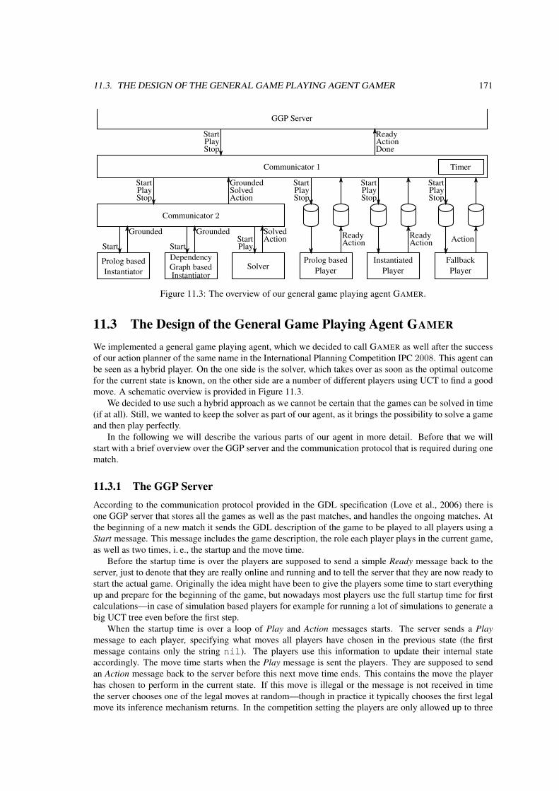
11.3. THE DESIGN OF THE GENERAL GAME PLAYING AGENT GAMER 171
GGP Server
StartPlayStop
ReadyActionDone
Communicator 1 Timer
StartPlayStop
GroundedSolvedAction
Communicator 2
Start
Grounded
Prolog basedInstantiator
DependencyGraph basedInstantiator
SolverProlog based
PlayerInstantiated
PlayerFallbackPlayer
Start
Grounded
PlayStart
SolvedAction
StartPlayStop
ReadyAction
ReadyAction Action
StartPlayStop
StartPlayStop
Figure 11.3: The overview of our general game playing agent GAMER.
11.3 The Design of the General Game Playing Agent GAMER
We implemented a general game playing agent, which we decided to call GAMER as well after the successof our action planner of the same name in the International Planning Competition IPC 2008. This agent canbe seen as a hybrid player. On the one side is the solver, which takes over as soon as the optimal outcomefor the current state is known, on the other side are a number of different players using UCT to find a goodmove. A schematic overview is provided in Figure 11.3.
We decided to use such a hybrid approach as we cannot be certain that the games can be solved in time(if at all). Still, we wanted to keep the solver as part of our agent, as it brings the possibility to solve a gameand then play perfectly.
In the following we will describe the various parts of our agent in more detail. Before that we willstart with a brief overview over the GGP server and the communication protocol that is required during onematch.
11.3.1 The GGP ServerAccording to the communication protocol provided in the GDL specification (Love et al., 2006) there isone GGP server that stores all the games as well as the past matches, and handles the ongoing matches. Atthe beginning of a new match it sends the GDL description of the game to be played to all players using aStart message. This message includes the game description, the role each player plays in the current game,as well as two times, i. e., the startup and the move time.
Before the startup time is over the players are supposed to send a simple Ready message back to theserver, just to denote that they are really online and running and to tell the server that they are now ready tostart the actual game. Originally the idea might have been to give the players some time to start everythingup and prepare for the beginning of the game, but nowadays most players use the full startup time for firstcalculations—in case of simulation based players for example for running a lot of simulations to generate abig UCT tree even before the first step.
When the startup time is over a loop of Play and Action messages starts. The server sends a Playmessage to each player, specifying what moves all players have chosen in the previous state (the firstmessage contains only the string nil). The players use this information to update their internal stateaccordingly. The move time starts when the Play message is sent the players. They are supposed to sendan Action message back to the server before this next move time ends. This contains the move the playerhas chosen to perform in the current state. If this move is illegal or the message is not received in timethe server chooses one of the legal moves at random—though in practice it typically chooses the first legalmove its inference mechanism returns. In the competition setting the players are only allowed up to three

172 CHAPTER 11. PLAYING GENERAL GAMES
errors (too late answers or illegal moves) in a single match; if they do more their score for this match willbe set to zero, no matter the reward they actually get in the terminal state. Once the server has received orchosen moves for all participating players it sends another Play message.
When the moves of the players result in a terminal state the server sends a Stop message instead of aPlay message. This again contains the moves chosen by all the players, so that the players might use this tocalculate the final state and determine the outcome of the game. When they are done they are supposed tosend an empty Done message to the server to denote that they are done with this match and ready to startthe next one.
In the first few competitions a GGP server of the Stanford games group36 was used, later one of TUDresden37 and in the last competition one by Sam Schreiber38. The latter two are open source and can bedownloaded and installed in order to start a server on a personal machine.
11.3.2 The Communicators
We use two communicators, one to interface between the players and the server, another to interface betweenthe first communicator and the solver and instantiators.
When a new Start message is received the first communicator starts the Prolog based player as well asa fallback player (Section 11.3.5), which is only important if something goes wrong in the normal players.It also sets a timer which will fire a short time before the startup time is over and during the normal playbefore a play time is over, so that an answer can be sent to the server in time.
Additionally it informs the internal second communicator that a new game is to be started.This second communicator immediately starts the two instantiators (Section 11.3.3). When one of those
is finished the communicator stops the other instantiator, starts the solver (Section 11.3.4) and informsthe first communicator (by sending a Grounded message). If this message is received before the startuptime is over that one stops the Prolog based player and instead starts the player using instantiated input(Section 11.3.5). When the solver is finished the second communicator sends a Solved message to the firstcommunicator, which stops all running players, because from now on optimal moves according to the foundsolution can be played.
The Play and Stop messages are forwarded from the first communicator to the second one, which usesthese to update the solver. The communication to the players is a bit more complicated, as somehow wedid not get the network communication to work reliably between the communicator (implemented in Java)and the players (implemented in C++), so that we decided to switch over to the use of files on the hard disk.Thus, for each Play message a file containing the moves is created, which is evaluated by the players. Theyalso inform the communicator of the move to take via files. The players write the best move so far wheneverit changes, and the communicator reads it when the move time is over.
11.3.3 The Instantiators
As we have seen in the experimental evaluation of our two approaches to the instantiation of general games(Section 9.2 both ways of instantiating have their advantages and drawbacks, and we are not yet able toautomatically determine when one will work better than the other. Thus, we decided to actually start bothinstantiators in parallel.
When one instantiator is finished it sends a Grounded message to the internal (second) communicator,which then does three things. First, it stops the other instantiator, so that more memory can be used by otherprocesses, because the result of that is no longer important. Second, it starts the solver. Third, it relays themessage to the outer (first) communicator, which in turn stops the Prolog based player and starts the oneworking on the instantiated input in case the startup time is not yet exceeded.
36http://games.stanford.edu37http://ggpserver.general-game-playing.de38http://code.google.com/p/ggp-base

11.3. THE DESIGN OF THE GENERAL GAME PLAYING AGENT GAMER 173
11.3.4 The SolverWhen the game at hand is fully instantiated and the solver has started the internal communicator informs itof all the moves that have been done so far, if any. The solver generates all the necessary BDDs, i. e., forthe initial state, the transition relation, the termination criterion, and the reward rules. Then it applies themoves that were already performed to end up in the current state. When this is done it starts the forwardsearch at that state. The idea behind this is that we do not care about a strong solution for those states thatcannot be reached any more, but rather prefer to save some time in the solving process. Any step alreadyperformed might decrease the solving time drastically.
We might omit the forward search completely if we decided to use the strong pre-image based approachto solve the games. Nevertheless, in the evaluation of the solvers in Section 10.4.2 we saw that omitting theforward search actually harms the solution process as the runtime often increases a lot. Thus, we decided touse forward search anyway. Given this decision and the results of the layered approach to solving generalgames we further decided to use the layered approach, as this is not only faster but allows for faster checkingif the current state has already been solved.
When the forward search is completed and the actual solving starts, after each backward step the solverchecks if the current state has already been solved. Due to the layered approach all it has to do is comparethe index of the last solved layer with the layer of the current state. To know the current layer the solverneeds only count the number of moves already performed, i. e., the number of Play messages it has received.
Once it has found that the current state is solved it first of all informs the internal communicator aboutthis by sending a Solved message. The communicator relays the message to the outer communicator whichstops all players that might still be running, because with the solution for the current state and all possiblyreachable successor states found we can play optimally as long as we follow the moves the solver sends.
To find the moves the solver searches the BDDs containing the solution of the current layer for thecurrent state. From the filename it can determine the optimal outcome. In order to choose an optimal moveit applies one move legal after the other until it has found one that results in a successor state that is part of aBDD of the solution achieving the same result in the successor layer. Here we make use of the fact that westored the terminal states and the non-terminal states in different files. In case we do not get the maximalreward of 100 we will always stick to a move that results in a non-terminal state if that is possible withoutdecreasing the calculated reward, hoping that the opponent will make a mistake enabling us to get a betterreward. Given a chosen move it sends the corresponding Action message to the internal communicator,which relays it to the outer communicator, which in turn relays it to the server. The next Play messageis relayed to the solver, which updates its current state, finds it in the solutions of the current layer, andproceeds as before. This is repeated until the game ends.
11.3.5 The PlayersApart from the solver we have three independent players to find a good move, one based on Prolog, anotherbased on the instantiated input, and another one that is merely a fallback in case something goes completelywrong, so that at least some legal move will still be sent to the server.
The Prolog Based Player
The Prolog based player is a UCT player that uses Prolog to evaluate the formulas, i. e., find the legal movesin the current state, calculate the successor state and check if the state is terminal and which rewards theplayers get in such a case. For the logic evaluation we decided to use SWI Prolog39, which provides aninterface to C++, in which we implemented our player.
For opponent modeling in multiplayer games, we use as many UCT trees as there are players, similarto the approach by Finnsson and Bjornsson (2008). In each tree we perform UCT from the correspondingplayer’s point of view. The advantage of this approach over one modeling all players within the same treeis two-fold. First, in case of simultaneous move games we need fewer nodes. For a state where we have nactive players with m legal moves per player, storing all possibilities in one tree would need mn successornodes, while we need only m nodes in each of the n trees. Second, using only one tree we normally would
39http://www.swi-prolog.org

174 CHAPTER 11. PLAYING GENERAL GAMES
need to calculate the average reward achieved when choosing a specific move by each player, so that wewould have to combine the averages of several of the successors into one value, which would also be muchmore time consuming, as this is done automatically in each of the trees in our approach. Nevertheless, thisapproach also comes with a disadvantage, as we do not know the exact successor state given one player’smove, so that we must use Prolog to calculate the successor state in every step within the UCT trees andcannot simply store a pointer to the successor as it might be done in the setting of only one tree for allplayers.
We found that Prolog’s inference mechanism is rather slow in most games (we provided some resultsfor pure Monte-Carlo search in Table 9.1 on page 118 for motivating the use of an instantiator), so that wedo not only store the first new state of a Monte-Carlo run in the tree but rather the complete run if the movetime is below a certain threshold—45 seconds seems to be a reasonable compromise. If the move time israther short, the player performs only relatively few runs, so that there is no harm in storing the full runsin terms of memory, i. e., we do not run out of memory, but we can store more information which shouldhelp to perform better than with only one added state. If the move time is longer than the threshold we areable to perform more runs, so that the memory might run out if we stored all runs completely. Due to theincreased number of runs we still extend the tree reasonably when only adding one new state per run so thatin that case we still should be able to find good moves.
We also implemented parallelization. Unfortunately, we did not find a way to get SWI Prolog to workin a shared memory approach, because the knowledge bases of the different threads got mixed up. Thus,we decided to use independent processes and the message passing interface MPI, in this case Open MPI40
(Gabriel et al., 2004), to send the messages between them. Due to this we are restricted to those paralleliza-tions that do not share any memory, especially the root parallelization or the at-the-leaves parallelization,but this way we are in principle able to run our player on a large cluster of computers, though so far weplayed only on one (multi-core) machine.
We implemented an approach close to the root parallelization proposed by Cazenave and Jouandeau(2007). The master stores only the root of the tree along with the immediate successor nodes, as in thesethe counters and the averages of the corresponding moves are stored. The slave processes each have theirown UCT trees and perform normal UCT. After each run they inform the master about the chosen movesand the achieved rewards for the players. The master takes this information and merges it into its nodes.After each update it checks if the best action has changed. If that is the case, it writes it into a file so thatthe communicator can read it once the time is up.
When the communicator informs the master about the chosen moves of all the players it broadcaststhis information to all the slaves. Furthermore, it updates its tree by setting the chosen successor nodesas the new roots and generating their successors. Next it receives the number of visits and the averagerewards for each successor from each slave. Based on this information it then calculates the total averagesand broadcasts these to the slaves, so that those can start the search for the next move to play with a moreinformed root node.
The only difference between single- and multiplayer games comes with the fact that for single-playergames we know that when we have found a path leading to the maximal reward of 100 points we havefound an optimal solution, so that we stop the algorithm and submit these moves, one after the other, to thecommunicator.
We also implemented a simple version of a transposition table. This takes a state in form of a stringas the key and returns the corresponding node within the UCT tree, if it exists. The advantage is of coursethat we need less memory than without it, as we do not need to store duplicates any longer. Also, theinformation generated on different paths traversing over the same state is combined in that state, so that itshould be more precise.
The Instantiated Player
The UCT player that uses the instantiated input consists of three different approaches. We have UCTversions for single-player games, for non-simultaneous multiplayer games and for simultaneous multiplayergames.
40http://www.open-mpi.org

11.3. THE DESIGN OF THE GENERAL GAME PLAYING AGENT GAMER 175
All versions are parallelized using C++ pthreads, so that we can make use of the shared memory. Aslong as we use only a single machine this is a reasonable approach. We use the algorithm previouslydescribed by Edelkamp et al. (2010a), which is similar to Chaslot et al.’s (2008a) tree parallelization withvirtual loss.
We use a static allocation of a UCT tree, i. e., we allocate the memory for the nodes of the tree at thestart of the algorithm and will never allocate new nodes afterward. The tree here is represented by an arrayof nodes, so that we can access a certain node by its index within the array. Each node stores the indices ofthe successor nodes—here some additional memory must be allocated at runtime—as well as their number,the average reward for each player, the number of times this state has been expanded, the hash value of thisstate, and—in case of a non-simultaneous multi-player game—the index of the player active in this state.
Additionally we store a hash table and a state table. The hash table stores the index of the noderepresenting the state having the given hash value, while the state table stores the corresponding state.We use the hash table as a kind of transposition table in order to remove duplicates. Whenever a supposedlynew state is to be inserted into the tree, we first of all calculate its hash value. For this we apply doublehashing, i. e., we use two hash functions h1 and h2 and check both the hash table starting at positionsh1+ i×h2 mod size with size being the size of the tables, a large prime number (in our case 201,326,611),and i ≥ 1 an integer to successively check different buckets. If the hash table has stored an index at thetested location, and it is the same state—which we can find out by checking the state table—we are done,as the state already is inserted in the tree. If the hash table has stored an index but the corresponding statediffers from the new one we continue with the next bucket (by incrementing i). Otherwise, if the hash tablehas not stored an index at that location this state is new and the corresponding node can be added to theUCT tree, i. e., at the position of the next unused index. This index is also added to this position of the hashtable and the actual state to the same position of the state table.
To handle the parallel accesses to the various tables we need two mutexes, one on the index of the nextempty position in the UCT tree, and another one on the hash table. When we have reached a leaf of theUCT tree and expand it, we first check if the newly generated successor is really a new state, as we havedescribed before, and lock the hash table so that no other process may access it at the same time. If it is nonew state we unlock the hash table and then must only set the index of the successor correspondingly andcontinue the search within the tree to the next leaf. Otherwise we update the hash and state table, unlockthe hash table, generate a new node for the new state, lock the index of the next empty position in the UCTtree, add the node to this position, increase the index to the next empty position and unlock it again. Thisway only processes that want to add new nodes at the same time may collide and they can only operatesequentially, while all other processes can continue their work undisturbed in parallel.
In the single-player version we store not only the average reward achieved but also the maximal rewardever found on this path. For the UCT search we randomly decide if we use the average score or the maximalscore in the UCT formula. When writing the best move into the file for the communicator we always choosethe move with the highest maximal reward.
During the instantiation process we already find out if a multiplayer game contains simultaneous movesor not, so that we can handle the two cases differently in this player. In contrast to our Prolog player, innon-simultaneous games we manage only one UCT tree. As in each state only one player can choose amove, we just have to check who is the active player in the state that is represented by the current node.For this we check the first successor node, which contains a pointer to the move that leads to it. This movestores the information who is the active player. For this player we then calculate the UCT values and choosethe move with maximal value. Once the movetime is up, we choose the move for which we achieved thehighest average reward.
The games containing simultaneous moves are handled similarly. Instead of combining all the succes-sors with the same move for one of the players to generate the total average by choosing that move wesimply set the active player randomly and then use the algorithm for turn-taking games, i. e., we choose themove with highest UCT value for that player. Because we choose the active player at random every timewe reach a node we hope that overall the move that is best for all players will be chosen more often thanthe others, though of course we sacrifice a lot of possibly useful information in order to further speed up thesearch.

176 CHAPTER 11. PLAYING GENERAL GAMES
The Fallback Player
The last part of the complete agent is the fallback player. This is not actually a true player, but is merelyused in case of an emergency.
Internally it stores the current state and updates it with each Play message that is received. Aftersuch an update it writes all the legal moves, which it finds by querying Prolog, into a file, which the firstcommunicator will read. Before sending the next move to be taken to the server it checks if that move isone of those found to be legal by the fallback player. If it is, everything is fine. Otherwise there is either nomove to be sent or it is not legal, so that some bug might have occurred. To still be able to achieve at leastsome points the communicator then chooses one of the legal moves at random and sends that to the server.If an error occurs early in the game that of course is a problem, and we will likely only play random movesfrom then onwards, so that we will have rather bad chances for achieving a good terminal state and gaininga high reward. If an error occurs later on it might very well be that random moves will suffice so that wewill still get some points. Ignoring the information that a move is illegal and sending it anyway, or sendingno move whatsoever, would result in an error of the agent; if an agent produces more than three errors, itgets no points, no matter the terminal state, so that sending random moves might actually help in such acritical case.
11.4 Experimental EvaluationWe performed a number of experiments with our player on our machine, i. e., an Intel Core i7 920 CPUwith 2.67GHz and 24GB RAM. The CPU is a quad-core CPU, but is treated by the operating system as anoct-core due to Hyperthreading.
In a first set of experiments (Section 11.4.1) we used only the Prolog based player and evaluated theeffect of an increased number of threads on the total number of UCT runs and on the initial evaluation.Then we performed the same set of experiments using the instantiated player (Section 11.4.2). Finally, for anumber of single- and non-simultaneous two-player games we evaluated the overall hybrid player (Section11.4.3).
11.4.1 Evaluation of the Prolog Based Player
Here we are only interested in the influence that an increased number of threads or an increased runtimehas on the average reward that is stored at the root node. Note that this average reward does not necessarilyreflect the reward that will be reached when stopping the search and playing only based on the informationalready gathered. Especially in case of single-player games this value might be a lot smaller than one wouldexpect, if many different terminal states result in a low reward and only few in a higher reward. However,the hope is that this average will increase the longer the player runs or the more threads are used to performthe UCT search. Even if the average value does not change too much over time we still can be certain thatmore runs generate a larger UCT tree, so that they will bring an advantage in the long term.
We evaluated the Prolog based player on six different games, three single-player games, namely FROGSAND TOADS, PEG-SOLITAIRE, and MAX KNIGHTS, as well as three non-simultaneous two-player games,namely CLOBBER (on a 4× 5 board), CONNECT FOUR (on a 7× 6 board), and SHEEP AND WOLF.
Before we get to the results, let us briefly describe the used games. PEG-SOLITAIRE, CLOBBER, andCONNECT FOUR were already described in the course of this thesis. FROGS AND TOADS, which is basedon Loyd’s FORE AND AFT puzzle (1914, p. 108), is played on a board consisting of two overlapping squaredboards. Each board has an edge length of four cells and they overlap on one cell (cf. Figure 11.4). The frogs(here denoted by black circles) start on the left board, the toads (the white circles) on the right board. Thegoal is to swap the positions of the frogs and the toads. To achieve this the player may either move a pieceto an adjacent cell if that is empty or jump over another piece onto an empty cell. Note that no pieces areever removed, so that only one cell is empty throughout the game. According to Yucel (2009) it takes atleast 115 steps to achieve the goal. In the GDL specification the game ends after 116 steps or if the desiredgoal is reached. The player gets a reward correlated to the number of pieces on the correct side of the board,so that a total of 31 different rewards are possible.

11.4. EXPERIMENTAL EVALUATION 177
Figure 11.4: The game of FROGS AND TOADS.
The game MAX KNIGHTS was first used at the 2009 GGP competition. It is played on an 8 × 8 chesslike board and the goal is to place as many knights on the board as possible. Similar to the QUEENS puzzlethe idea is to place the knights in such a manner that they cannot capture each other. Once a knight is placedin a cell that is attacked by an already placed knight the game ends. Of course, for a human this game israther trivial. At most 32 knights that cannot capture each other can be placed on the board, as they canonly capture pieces on cells of the other color. Thus, it is save to place them all on cells of the same color..In the GDL specification of this game the player gets a reward correlated to the number of placed knights,i. e., a32 different reward values are defined.
The game SHEEP AND WOLF is also played on an 8 × 8 chess like board, though in this game onlythe black cells are used. Initially, four white pieces (the sheep) are placed in the bottom row and one blackpiece (the wolf) in the topmost row. The sheep can only move forward one cell at a time, the wolf can moveforward or backward, but also only one cell at a time. The wolf performs the first move. The goal for thesheep is to prevent the wolf from being able to move. Thus, if all adjacent cells are occupied by sheep thewolf has lost.41 The goal of the wolf is just the inverse, i. e., it has to try to escape the sheep. The gameends when either the sheep have completely surrounded the wolf or the wolf has escaped. As the sheep canonly move forward it is clear that the game ends after at most 56 moves, when all sheep have reached thetopmost row. Again, this game is rather trivial for a human, as the sheep can always move in such a waythat the wolf cannot get behind them, so that at the end they will be able to push it back to the topmost rowand to occupy the adjacent cells. However, a simulation based player may quickly run into trouble becausethere are only relatively few terminal states that are won by the sheep while many playouts lead to the wolfescaping. The GDL specification distinguishes only between won and lost states, i. e., only two rewardcombinations are possible.
Concerning the possible rewards, in PEG-SOLITAIRE the player is awarded a number of points reverselycorrelated to the number of remaining pieces on the board (100 for one piece in the middle, 99 for one piecesomewhere else, 100− i for 1 + i pieces left on the board, with a minimum of 0 points for eleven or morepieces). In CLOBBER the players get a reward dependent on the number of moves it took them to finish thegame. If the starting white player performed the last move it gets roughly 14i points if i white pieces arestill on the board; if the black player performed the last move it gets roughly 16i points if i black piecesare still on the board. The losing player always gets zero points. CONNECT FOUR is a typical two-playerzero-sum game with only won, lost, or drawn terminal states, so that only three reward combinations arepossible.
All games are at least weakly winnable for all players, i. e., 100 points are possible if they all cooperatein order to maximize that player’s points. Thus, for all single-player games it is possible to reach a terminalstate with a reward of 100 points, while for the two-player games the outcomes are 42–0 in CLOBBER,100–0 in CONNECT FOUR, and 0–100 in SHEEP AND WOLF if both players play optimally. All two-playergames were evaluated from the point of view of the starting player.
41In other words, the sheep hunt the wolf. This sounds strange, but that is what this game is about.

178 CHAPTER 11. PLAYING GENERAL GAMES
0
10000
20000
30000
40000
50000
60000
70000
80000
90000
0 20 40 60 80 100 120
Num
bero
fRun
s
Runtime [s]
1 Thread2 Threads3 Threads4 Threads5 Threads6 Threads7 Threads8 Threads9 Threads
10 Threads
Figure 11.5: Number of UCT runs in CLOBBER by the Prolog based player, averaged over 10 runs.
Table 11.1: Number of UCT runs of the Prolog based player after two minutes, averaged over 10 runs.
Game 1 Thread 2 Threads 3 Threads 4 Threads 5 Threads 6 ThreadsFROGS AND TOADS 745 761 1,511 2,256 2,482 2,531
MAX KNIGHTS 25,970 26,164 51,773 77,179 81,861 88,891PEG-SOLITAIRE 7,917 8,138 15,925 23,770 25,260 28,401
CLOBBER 21,881 21,853 43,635 64,560 73,151 76,123CONNECT FOUR 19,638 19,844 38,808 57,811 65,263 68,393
SHEEP AND WOLF 4,514 4,720 9,322 13,929 14,921 16,134
Number of Runs
Figure 11.5 depicts the number of UCT runs for varying number of threads during two minutes in the gameCLOBBER. The first thing to notice is that the number of runs does not really differ between the use of oneand two threads. This is due to the parallelization we chose. For the root parallelization we have a masterprocess and a number of slave processes, which are the only ones that actually perform UCT runs, while themaster process collects the results of all the slaves. In the case of a single thread we use a version withoutany parallelization, i. e., the only process performs all the searches and no master is necessary to collect theresults. Thus, the cases for one and two threads are very similar.
Additionally it can be noted that using three threads, i. e., two slaves, the player can perform about twiceas many runs as with only one or two threads, i. e., one slave. Similarly, for four threads, i. e., three slaves,the number of runs is increased to a factor of roughly three compared to the single slave version. For fiveand six threads, i. e., more than we have physical cores, there is still an increase, but it is less prominent.From then on the increase in number of runs gets smaller and smaller, so that for the later experiments wedecided to stick to a setting with up to six threads.
In our implementation we have to call Prolog even from within the UCT tree, so that the runtime doesnot differ much between smaller or bigger UCT trees. Thus, it is plausible that for any number of threadsthe number of UCT runs increases linearly with the total runtime, which can be clearly seen from the figure.
We performed the same experiment for the other games as well, and all results look very similar. Thus,we do not provide the graphs but only the total number of runs performed after two minutes (cf. Table 11.1).
Single-Player Games
Concerning the average reward determined for the initial state the results are also similar for all six testedgames, but actually quite unexpected. In all cases the number of threads has no big influence on the overall

11.4. EXPERIMENTAL EVALUATION 179
2.5
3
3.5
4
4.5
5
5.5
0 20 40 60 80 100 120
Ave
rage
Rew
ard
Runtime [s]
1 Thread2 Threads3 Threads4 Threads5 Threads6 Threads
Figure 11.6: Average rewards for FROGS AND TOADS by the Prolog based player, averaged over 10 runs.
4.25
4.3
4.35
4.4
4.45
4.5
4.55
4.6
0 20 40 60 80 100 120
Ave
rage
Rew
ard
Runtime [s]
1 Thread2 Threads3 Threads4 Threads5 Threads6 Threads
Figure 11.7: Average rewards for MAX KNIGHTS by the Prolog based player, averaged over 10 runs.
evaluation. Neither does it influence the time needed to reach a reasonably stable point, i. e., one where theaverage reward does not change much any more.
The length of the game steps makes FROGS AND TOADS rather complex. Due to this only few UCTruns can be performed (745 in two minutes for one thread), but still the results are very stable, even afterabout ten seconds (cf. Figure 11.6). Independent of the number of threads the average reward achieved isclose to 3.5. An explanation for this bad result might be the complexity of the game, because there aremany possible runs, and only very few result in a good outcome. In the random Monte-Carlo runs it mightvery well be that the player performs only moves or jumps within the square of pieces of the same colorinstead of trying to really swap sides. However, these are only the average rewards. Thus, playing based onthe information already gathered after 120 seconds should enable the player to reach a much higher reward.What is quite surprising is that here an increased number of threads (and thus runs) slightly decreases theoverall average reward. An explanation might be that at first more runs mean that larger parts of the gameare analyzed, and thus more terminal states with lower rewards are found. It might be that with a lot moreruns the UCT tree grows enough to guide the search to better terminal states more reliably.
At first glance the results for MAX KNIGHTS seem to show a rather strange behavior (cf. Figure 11.7).Here the average oscillates with a decreasing amplitude before finally settling at an average of roughly

180 CHAPTER 11. PLAYING GENERAL GAMES
34.5
35
35.5
36
36.5
37
37.5
38
38.5
39
39.5
0 20 40 60 80 100 120
Ave
rage
Rew
ard
Runtime [s]
1 Thread2 Threads3 Threads4 Threads5 Threads6 Threads
Figure 11.8: Average rewards for PEG-SOLITAIRE by the Prolog based player, averaged over 10 runs.
4.35 after about 80 seconds. With more threads the amplitude gets smaller. Nevertheless, for all cases itis actually quite small; the difference between the first two extrema is less than 0.2 points, so that there isnot much difference, especially given the fact that here 100 points are optimal and the achieved averagecorresponds to the situation of having placed only five or six knights. Note that according to the GDLspecification of this game it is actually possible to place a new knight anywhere on the board and onlyafter a move it is determined whether the game ends (if the newly placed knight can capture one of the olderones), so that the random choice in the Monte-Carlo runs might again be an explanation for this bad averagevalue. The more knights are already placed on the board the higher the probability to choose a move thatresults in the end of the game.
For PEG-SOLITAIRE (cf. Figure 11.8) the overall behavior is again similar to the first games. Afterroughly 20 seconds most versions are quite stable between 35.5 and 36 points. Only the versions with oneand two threads take longer, and the determined average reward for both cases is still increasing after thetimeout of two minutes. Also, their results are a bit below all the others throughout the complete runtime.In this case, if more threads are used then the results are a bit better, but again the difference is rather small.From the achieved average value it seems that in PEG-SOLITAIRE lots of playouts actually lead to terminalstates achieving many points.
Two-Player Games
For the two-player games we assume that we are the starting player and thus the average reward correspondsto the average outcome of the first player in the terminal states that were reached during the UCT runs.
For CLOBBER (Figure 11.9) after 40 seconds the stable point is reached, and independent of the numberof threads the achieved average reward is around 34.5 points. From the beginning the results did not differmuch, as even from the first second of search onwards they were between 32 and 35.5. Given that the firstplayer can achieve a reward of 42 in case of optimal play of both players the results of the UCT runs areactually quite close to the optimal estimate.
In CONNECT FOUR (Figure 11.10) the results differ a bit more than in CLOBBER. After about 80 sec-onds the version using only one thread and after about 40 seconds all other versions achieved a reasonablystable point where the average reward lies between 57 and 59 points. In this game the number of threads in-fluenced the average outcome negatively again, as with more threads the average value is slightly decreased.However, this difference again might not be significant enough to allow strong conclusions.
As we have mentioned earlier, for a human the game SHEEP AND WOLF is rather easy to solve, whilefor a computer player, at least one based on UCT searches, this seems to be much more difficult (cf. Figure11.11). Independent of the number of threads, the average reward achieved in the initial state lies between

11.4. EXPERIMENTAL EVALUATION 181
32
32.5
33
33.5
34
34.5
35
35.5
0 20 40 60 80 100 120
Ave
rage
Rew
ard
Runtime [s]
1 Thread2 Threads3 Threads4 Threads5 Threads6 Threads
Figure 11.9: Average rewards for CLOBBER by the Prolog based player, averaged over 10 runs.
53
54
55
56
57
58
59
60
61
0 20 40 60 80 100 120
Ave
rage
Rew
ard
Runtime [s]
1 Thread2 Threads3 Threads4 Threads5 Threads6 Threads
Figure 11.10: Average rewards for CONNECT FOUR by the Prolog based player, averaged over 10 runs.
90 and 95 points for the first player (the wolf), and is stabilized between 91 and 92 points after about 30seconds. The explanation here clearly is that most lines of play lead to the wolf actually being able to getpast the sheep, and only quite few prevent that from ever happening, and these playouts thus dominate theaverage reward found by the UCT player.
11.4.2 Evaluation of the Instantiated PlayerFor the instantiated player we used the same set of experiments, i. e., first experiments to find the influenceof the number of used cores (ranging again from one to ten) on the number of UCT runs within two minutesfor the six games used before, then the influence of the number of cores on the average (or maximal in caseof single-player games) rewards within two minutes for the six games.
Number of Runs
Concerning the number of UCT runs we again show only one graph to show the influence of the number ofthreads over time (cf. Figure 11.12), because for all games the situation is very similar.

182 CHAPTER 11. PLAYING GENERAL GAMES
89
90
91
92
93
94
95
96
0 20 40 60 80 100 120
Ave
rage
Rew
ard
Runtime [s]
1 Thread2 Threads3 Threads4 Threads5 Threads6 Threads
Figure 11.11: Average rewards for SHEEP AND WOLF by the Prolog based player, averaged over 10 runs.
0 · 100
1 · 106
2 · 106
3 · 106
4 · 106
5 · 106
6 · 106
0 20 40 60 80 100 120
Num
bero
fRun
s
Runtime [s]
1 Thread2 Threads3 Threads4 Threads5 Threads6 Threads7 Threads8 Threads9 Threads
10 Threads
Figure 11.12: Number of UCT runs in CLOBBER by the instantiated player, averaged over 10 runs.
For one thread we get a linear increase in the number of runs with the time played. Though here westore the states within the UCT tree it seems that the overhead required by the Monte-Carlo runs, where theset of legal moves and the successor states must be calculated, is not too big, especially compared to thesituation when using Prolog. Otherwise, we would expect to see more than a linear increase in the numberof runs over time.
In this setting, when using two threads we gain more than a factor of two in the number of runs. This islikely because in all cases we use only one thread to determine the best move and write it to the hard diskwhenever it has finished a UCT run. This way, only one thread is slowed down while the others can operateat full speed running only the UCT runs.
For three threads we arrive at roughly 1.5 times the number of runs as in the two thread setting, for fourthreads we can double the number of runs. From then on the increase is a lot smaller, similar to the settingin the Prolog based player.
In the other games the situation looks very similar, and the main difference comes with the number ofruns for the different games. The results after two minutes are depicted in Table 11.2.
Compared to the Prolog based player we can see a clear improvement in the number of runs, rangingfrom a factor of 34 in FROGS AND TOADS to 180 in MAX KNIGHTS, though the numbers are not really

11.4. EXPERIMENTAL EVALUATION 183
Table 11.2: Number of UCT runs of the instantiated player after two minutes, averaged over 10 runs.
Game 1 Thread 2 Threads 3 Threads 4 Threads 5 Threads 6 ThreadsFROGS AND TOADS 20,421 38,550 55,262 72,105 79,592 86,800
MAX KNIGHTS 3,132,020 5,879,737 8,649,243 10,885,410 11,784,900 12,547,157PEG-SOLITAIRE 1,158,908 2,162,479 3,254,122 4,306,140 4,753,630 5,123,357
CLOBBER 611,022 2,078,154 3,234,853 4,174,324 4,587,748 4,934,097CONNECT FOUR 1,495,015 2,912,314 4,280,195 5,721,257 6,108,360 6,633,747
SHEEP AND WOLF 250,920 536,415 809,008 1,071,300 1,128,661 1,196,076
comparable as the algorithms do not only differ in the inference mechanism, but also in the used datastruc-tures.
Single-Player Games
Concerning the average and maximal rewards, we again compared only the use of one to six threads, as wehave seen that more threads do not bring too much more runs, and thus the average rewards will not differmuch.
For the average rewards of FROGS AND TOADS (cf. Figure 11.13a) the version using two threads getsstable after about 70 seconds, all the others after about 30 seconds, though there is not much differenceanyway. Initially, the average rewards were between 3.35 and 3.65, in the end they are close around 3.5independent of the number of used threads. Overall, the situation is very similar to one in the Prolog basedplayer.
Concerning the maximal rewards (cf. Figure 11.13b), which we store in the instantiated player as well,we can see that this value increases even at the timeout, though most increases happen during the first 40seconds. In the end, the maximal reward ever seen ranges from 24 to 27. Thus, in case of single-playergames it seems that this is a much better indicator of the reward that will be achieved in the end than theaverage, as the latter often clearly is negatively influenced by the runs that do not end in terminal statesachieving better rewards.
In the average rewards for MAX KNIGHTS (cf. Figure 11.14a) we again see some oscillating, similarto the Prolog based case, though here the amplitudes are even smaller. The more threads we use the fasterthe amplitude drops. Thus, for one thread it takes about 80 seconds, for two roughly 60 seconds, for threeabout 40 seconds and for the others between 20 and 30 seconds. Overall, the average rewards lie slightlyabove 4.3.
For the maximal rewards we see a similar picture (cf. Figure 11.14b) as we did for FROGS AND TOADS.Some increases occur even close before 120 seconds, though most happen in the first 40 or 60 seconds. Theversions using one and two threads are worse than the other versions throughout the runtime. At the end,one or two threads found a maximal reward of 28 points, the others one of 30 points.
Starting with an average reward between 35 and 35.1 in PEG-SOLITAIRE (cf. Figure 11.15) for anynumber of threads the average reward slightly increases the full runtime, though all the time the versionsusing more threads get a slightly higher average reward. After 120 seconds the averages range from 35.25to 35.45.
When looking only at the maximal rewards (cf. Figure 11.15b) we can see that during the first fiveseconds all versions found solutions achieving 90 points. With more time this value increases only slightlyup to at most 92. Thus, it must be easy even for simulation based approaches to find good solutions whereonly two pegs are left on the board, though a situation with only one peg left is a lot more difficult to find.Also, from the average values of more than 35 it seems that the number of situations with smaller rewardsis not as high as it seems to be in MAX KNIGHTS and FROGS AND TOADS.
Two-Player Games
For CLOBBER (cf. Figure 11.16) we can see that the results are quite stable after about 30 seconds in thesingle thread setting, though the average reward still increases slightly until the timeout. For more threads

184 CHAPTER 11. PLAYING GENERAL GAMES
3.35
3.4
3.45
3.5
3.55
3.6
3.65
0 20 40 60 80 100 120
Ave
rage
Rew
ard
Runtime [s]
1 Thread2 Threads3 Threads4 Threads5 Threads6 Threads
(a) Average rewards.
14
16
18
20
22
24
26
28
0 20 40 60 80 100 120
Max
imal
Rew
ard
Runtime [s]
1 Thread2 Threads3 Threads4 Threads5 Threads6 Threads
(b) Maximal rewards.
Figure 11.13: Average and maximal rewards for FROGS AND TOADS by the instantiated player, averagedover 10 runs.
the curves are very smooth already from only roughly five seconds onwards, but in those cases we can seea similar increase in the average values. Here we can see a difference between the number of threads. Themore threads we use the steeper the increase, though actually there is not much difference anyway. After120 seconds the player arrives at an average value between 34.4 and 34.9. Compared to the Prolog basedplayer we see that the averages became stable a lot faster, but the average rewards in the end are similar inboth settings.
For CONNECT FOUR (cf. Figure 11.17) we can again see a negative influence by increasing the numberof threads. When using more threads we arrive at a lower average value at the root node. In the one threadversion the average value still decreases at the timeout, while for the others after 60 to 90 seconds theaverage rewards are quite stable. Here, the averages range from 57.5 for six threads to 60 for one thread, sothat again the instantiated player’s results are similar to those of the Prolog based player.
In SHEEP AND WOLF the average values do not change much from the very beginning when using morethan one thread, though even when using only one the change is within 0.2 points. For more threads the
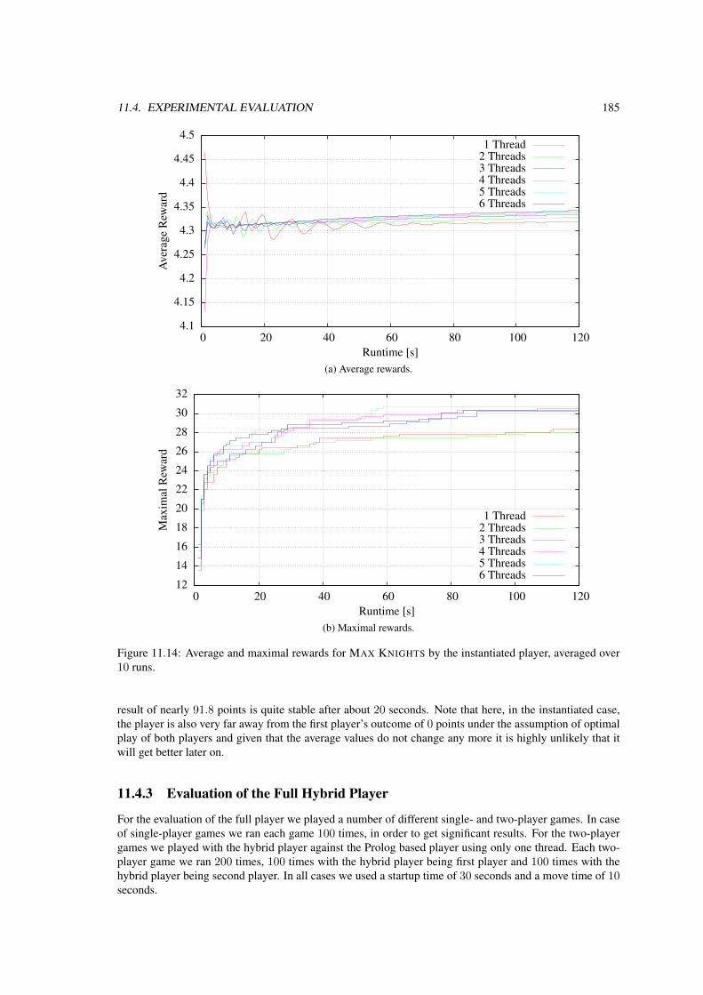
11.4. EXPERIMENTAL EVALUATION 185
4.1
4.15
4.2
4.25
4.3
4.35
4.4
4.45
4.5
0 20 40 60 80 100 120
Ave
rage
Rew
ard
Runtime [s]
1 Thread2 Threads3 Threads4 Threads5 Threads6 Threads
(a) Average rewards.
12
14
16
18
20
22
24
26
28
30
32
0 20 40 60 80 100 120
Max
imal
Rew
ard
Runtime [s]
1 Thread2 Threads3 Threads4 Threads5 Threads6 Threads
(b) Maximal rewards.
Figure 11.14: Average and maximal rewards for MAX KNIGHTS by the instantiated player, averaged over10 runs.
result of nearly 91.8 points is quite stable after about 20 seconds. Note that here, in the instantiated case,the player is also very far away from the first player’s outcome of 0 points under the assumption of optimalplay of both players and given that the average values do not change any more it is highly unlikely that itwill get better later on.
11.4.3 Evaluation of the Full Hybrid Player
For the evaluation of the full player we played a number of different single- and two-player games. In caseof single-player games we ran each game 100 times, in order to get significant results. For the two-playergames we played with the hybrid player against the Prolog based player using only one thread. Each two-player game we ran 200 times, 100 times with the hybrid player being first player and 100 times with thehybrid player being second player. In all cases we used a startup time of 30 seconds and a move time of 10seconds.

186 CHAPTER 11. PLAYING GENERAL GAMES
34.8
34.9
35
35.1
35.2
35.3
35.4
35.5
0 20 40 60 80 100 120
Ave
rage
Rew
ard
Runtime [s]
1 Thread2 Threads3 Threads4 Threads5 Threads6 Threads
(a) Average rewards.
80
82
84
86
88
90
92
0 20 40 60 80 100 120
Max
imal
Rew
ard
Runtime [s]
1 Thread2 Threads3 Threads4 Threads5 Threads6 Threads
(b) Maximal rewards.
Figure 11.15: Average and maximal rewards for PEG-SOLITAIRE by the instantiated player, averaged over10 runs.
As we have seen in the previous results, when using more than four threads the number of runs increasesonly slightly, from eight onwards there is no change whatsoever any more. Thus, we decided to use only oneto four threads for the hybrid player’s UCT algorithms, given that either the solver or the two instantiatorswould run in parallel anyway, so that we actually have five or even six threads running in parallel whenusing a UCT player with four threads.
Single-Player Games
For the single-player case we here used four different games. Beside FROGS AND TOADS, MAX KNIGHTS,and PEG-SOLITAIRE we also evaluated TPEG. The last one is nearly the same as PEG-SOLITAIRE, onlythat the initially empty cell is not in the middle of the board but one diagonally adjacent to it. Here, thereis no distinction for the places where the last peg resides, so that we get 100 − 10i points for i + 1 pegsstill on the board, with the minimum being 0 points for eleven or more pegs left. Additionally, the player is

11.4. EXPERIMENTAL EVALUATION 187
32
32.5
33
33.5
34
34.5
35
0 20 40 60 80 100 120
Ave
rage
Rew
ard
Runtime [s]
1 Thread2 Threads3 Threads4 Threads5 Threads6 Threads
Figure 11.16: Average rewards for CLOBBER by the instantiated player, averaged over 10 runs.
55
56
57
58
59
60
61
0 20 40 60 80 100 120
Ave
rage
Rew
ard
Runtime [s]
1 Thread2 Threads3 Threads4 Threads5 Threads6 Threads
Figure 11.17: Average rewards for CONNECT FOUR by the instantiated player, averaged over 10 runs.
Table 11.3: Results of the player for single-player games comparing different number of threads, averagedover 100 runs each, along with the 95% confidence intervals.
Game 1 Thread 2 Threads 3 Threads 4 ThreadsFROGS AND TOADS 41.63± 1.32 42.08± 1.45 46.16± 1.44 46.91± 1.27
MAX KNIGHTS 73.85± 2.97 70.70± 2.89 75.80± 2.70 74.35± 2.63PEG-SOLITAIRE 90.80± 0.60 91.50± 0.70 91.40± 0.68 91.80± 0.76
TPEG 97.40± 0.95 98.80± 0.64 98.30± 0.84 99.00± 0.59
allowed to commit suicide at any time, which immediately ends the game resulting in 15 points. The resultsfor these four games are depicted in Table 11.3.
We can see that for FROGS AND TOADS we get a significant increase from one to four threads. In thisgame, the instantiator finished after about two steps, but the solver never finished, so that the Prolog basedplayer was used the whole time.

188 CHAPTER 11. PLAYING GENERAL GAMES
90.6
90.8
91
91.2
91.4
91.6
91.8
92
0 20 40 60 80 100 120
Ave
rage
Rew
ard
Runtime [s]
1 Thread2 Threads3 Threads4 Threads5 Threads6 Threads
Figure 11.18: Average rewards for SHEEP AND WOLF by the instantiated player, averaged over 10 runs.
In MAX KNIGHTS the instantiator finished after 13 steps, but then the game was solved before the nextstep was done, so that the solver took over. From the results it seems that the Prolog based player playedsimilar in all cases until the game was solved.
The instantiation of PEG-SOLITAIRE finished even before the first step was done, so that the instantiatedplayer was started. The solver never finished, leaving the whole work to the player. In this game, the resultsdo not differ significantly between varying numbers of threads.
Finally, in TPEG the situation is similar to the one in PEG-SOLITAIRE, i. e., the instantiator finishedbefore the first step but the game was never solved, so that the whole time the instantiated player wasactivated. Here we see a small increase in the average outcomes from one to four threads. Of course, giventhat even for one thread we achieve 97.4 points on average prevents the versions using more threads toimprove too much over this. Nevertheless, the four threaded version achieves an average of 99.0 points.
Two-Player Games
For the two-player setting we used six different games, namely CHOMP, CLOBBER, CONNECT FOUR,CUBICUP, QUAD, and SHEEP AND WOLF. Apart from QUAD we have already introduced all of thesegames. The GDL descriptions of CHOMP and CUBICUP allow only for won and lost states, and also for adraw in case of CUBICUP, so that only two respectively three different reward combinations are possible.Overall, apart from CLOBBER all games are zero-sum games.
The game QUAD was orignally invented by G. Keith Still in 1979. It is played on an 11 × 11 board,where the four corners are missing. Each player has 20 pieces of its color (the quads) as well as sevenbarriers. During its turn a player may place as many barriers as it likes (and has left) and at the end onequad, then it is the other player’s turn. The goal is to establish a square spanned by four own quads (beingthe square’s corners), which may be upright or diagonal and of any size.
In the GDL description we use the board is smaller (7×7 cells without the corners) and each player getstwelve quads and five barriers. The game ends when a player has achieved one of three types of squares(depicted in Figure 11.19), namely a straight one with an edge length of two, a straight one with an edgelength of three or a diagonal one with an edge length of three. Alternatively, if no player was able toestablish an allowed square and no player has any quads left the game ends as well.
The game is defined to be zero-sum with six different reward combinations. In case one of the playershas established a square that player gets 100 points and the opponent 0. Otherwise if the starting player wasable to get a square nearly finished, i. e., three corners of an allowed square are placed, it gets 95 points andthe second player 5. In all the other cases the number of unplaced barriers of the players are important. If

11.4. EXPERIMENTAL EVALUATION 189
Figure 11.19: The game board of QUAD and the three allowed squares ending the game.
Table 11.4: Results of the player for two-player games comparing different number of threads, averagedover 100 runs each, along with the 95% confidence intervals. Results denoted by “—” mean that we didnot perform that experiment because the game was solved within the startup time, so that no difference inresults is to be expected.
Game 1 Thread 2 Threads 3 Threads 4 ThreadsCHOMP (1st player) — — — 100.00± 0.00
CHOMP (2nd player) — — — 99.00± 1.96CLOBBER (1st player) 39.24± 6.90 34.77± 7.04 47.85± 6.62 45.59± 7.28
CLOBBER (1st player’s opp.) 24.45± 5.90 30.68± 6.32 18.91± 5.63 22.42± 5.92CLOBBER (2nd player) 62.32± 4.76 58.5± 5.22 63.85± 4.41 60.00± 4.63
CLOBBER (2nd player’s opp.) 6.30± 3.57 8.46± 4.01 4.32± 2.91 5.15± 3.09CONNECT FOUR (1st player) 43.00± 9.75 57.50± 9.59 62.00± 9.56 61.00± 9.61
CONNECT FOUR (2nd player) 22.50± 8.17 23.00± 8.29 29.00± 8.94 40.00± 9.65CUBICUP (1st player) 31.00± 8.33 37.00± 8.77 50.50± 9.29 69.50± 7.87
CUBICUP (2nd player) 63.00± 8.77 67.00± 8.50 76.50± 7.81 86.00± 6.24QUAD (1st player) 68.90± 9.10 52.00± 9.84 63.00± 9.51 76.00± 8.41
QUAD (2nd player) 47.00± 9.83 40.00± 9.65 54.00± 9.82 56.00± 9.78SHEEP AND WOLF (1st player) — — — 53.00± 9.83
SHEEP AND WOLF (2nd player) — — — 100.00± 0.00
one player has more barriers left it gets 90 points and the opponent 10; if both have the same number ofunplaced barriers both get 50 points.
Most of the games are zero-sum games, so from the average outcome of the 100 games from one player’spoint of view the average outcome of the other is immediate. Only in case of CLOBBER, where we havemore general rewards, we cannot know both players’ rewards given only those of one, so that we provideall four results (for the hybrid player being first player and the opponent, as well as for the hybrid playerbeing second player and the opponent). All the average outcomes are depicted in Table 11.4.
In CHOMP the instantiator and the solver finish before the first step is performed. As the number ofthreads used is only relevant for the players we did not need to run this game for all settings of threads. Thegame is won by the first player, and thus our agent never loses if it is first player. Even if it is the secondplayer it wins 99% of the games, which shows that our Prolog based UCT player cannot handle it in a goodmanner and the idea to keep the solver waiting for a mistake by the opponent is beneficial, as otherwise itmight have chosen to take the last piece immediately and thus lost the game.
For the game of CLOBBER the instantiator finishes before the first step, so that instead of the Prologbased player the instantiated player is used for most of the runtime. In the settings of up to three threadsthe solver finishes a few steps before the game is over (often one to three steps). As the game ends when a

190 CHAPTER 11. PLAYING GENERAL GAMES
player cannot perform any more moves, and this might happen after varying number of steps, it seems thatin the four thread setting the player is able to reach a terminal after fewer steps.
The optimal outcome is 42 – 0, so that in case of one and two threads the player often plays suboptimal ifit is the first player, achieving only 39 and 35 points and allowing the seconds player to get 24 and 31 pointson average, respectively. Nevertheless, note that the optimal outcome of 42 points for the first player is stillwithin the 95% confidence interval in case of one thread. For three threads the situation gets significantlybetter, so that the player gets 48 points and the opponent only 19. For four threads the situation is similar,with 46 versus 22 points.
When taking the role of the second player, the instantiated player is a lot better. Here it is able to getaround 60 points in any setting, allowing the starting opponent to get only around six points. Surprisingly,here we see no significant influence by the number of used threads.
In CONNECT FOUR the instantiator finishes before the first step but the game is never solved, so thatonly the instantiated player is responsible for the moves. The optimal outcome is 100 – 0. In case the hybridplayer takes the starting player’s role, when using only one thread the player’s average is 43 points, so thatoverall the opponent wins more often. For two threads the average increases to 58, and for three and fourthreads the player is able to use its advantage and it plays significantly better than the opponent and arrivesat averages of 62 and 61 points.
Surprisingly, when playing the second player’s role, the situation looks bad for the hybrid player. Theachieved average outcome improves with a higher number threads, but even for four threads it reaches only40 points. This is clearly better than the optimal outcome, but still it seems that here the instantiated playerneeds four threads in order to play as well as the Prolog based player using only one thread, which is veryunexpected given the higher number of UCT runs—the instantiated player with four threads can performabout 290 times the runs the Prolog based player with one thread can perform.
For CUBICUP we do not know the optimal outcome, though at least from a UCT player’s point of viewit seems that the second player has an advantage, which might make sense as the first player must establishone more cubi cup than the second one in order to win. Similar to the situation in CONNECT FOUR, theinstantiator finishes before the first step but the solver never finishes. When using only one thread the hybridplayer achieves an average outcome of 31 points as first player and one of 63 points as the second player.When using more threads it plays significantly better, with the best rewards being 70 points as the firstplayer and 86 points as the second player when using four threads.
For QUAD, where the instantiator never finishes, the situation looks strange at first. Given only onethread the hybrid player achieves a higher average than with two threads. Actually, we would expect bothsettings to be similar, as in case of two threads actually only one thread performs the UCT searches, andthe average number of UCT runs is the same in both cases. When looking at the confidence intervals wesee that they overlap, so that we cannot be sure that the two threaded version really is worse than the singlethreaded one. When increasing the number of threads further, the results get better again, with 76 points asthe first player and 56 points as the second player for the four threaded version being the maximum.
In SHEEP AND WOLF the situation is similar to the one in CHOMP. Again the game is solved beforethe first step so that it is played optimally. As we have pointed out before, the game is won by the secondplayer, though UCT typically believes that it is a first player win. From the results we can see that the solvernever makes a mistake when being the second player, so that it consistently wins. When being first playerit cannot hope to win against an optimal player, but as UCT believes the game to be won by the first playerit clearly does not play optimal, so that 53% of the games are actually won based on the outcome of thesolving process.
11.4.4 Conclusion
So far, our UCT players are pretty basic. Most of the improvements such as MAST (Finnsson and Bjorns-son, 2008) or RAVE (Gelly and Silver, 2007) are not yet used in them. However, we can say that the hybridconcept works very well. In case a game can be solved before the first move is played, GAMER is clearlyable to use its advantage and plays optimally. Due to the decision to wait for an opponent’s mistake it oftenis able to win in games that it would lose if both players played optimally. Even if the solving takes longerit is able to play better than using only UCT.

11.4. EXPERIMENTAL EVALUATION 191
Concerning the number of runs the two UCT players scale nearly linearly when increasing the numberthreads or the runtime. Operating on a stronger machine with more processors or cores is thus very likelyto further increase the number of runs. Furthermore, we have seen that the use of the instantiated playergreatly increases the number of performed UCT runs compared to the Prolog based player. Even though theaverage rewards stored at the root node do not change much over time, the size of the UCT tree increaseswith each run, so that an increased number of runs often brings an advantage in practice.

192 CHAPTER 11. PLAYING GENERAL GAMES

Chapter 12
Conclusions and Future Work
The Road goes ever on and onDown from the door where it began,Now far ahead the Road has gone,And I must follow if I can,Pursuing it with eager feet,Until it joins some larger wayWhere many paths and errands meet.And whither then? I cannot say.
John R.R. Tolkien, The Fellowship of the Ring(The Lord of the Rings, Book 1)
To wrap up let us briefly recapitulate what this thesis was about. The overall topic was symbolic search,which we have applied in to AI topics, action planning and general game playing. Apart from some theo-retical results on the BDD sizes we have proposed a number of new algorithms or improvements of existingones.
For classical planning we have implemented an automated planner, which participated in two interna-tional planning competitions and was even able to win the first one. Though in the second competition itdid not fare as well we were able to further enhance it, so that now it can nearly cope with explicit heuris-tic search based planners, at least in the set of general action cost domains of IPC 2011. For net-benefitplanning we also implemented a new planner, which participated only in 2008 and was able to win thattrack.
For general game playing we have proposed an instantiator in order to get rid of the variables of theGDL input, so that its output can be used in symbolic search as well as in an explicit state player. Wheremost players so far resided to Prolog in order to infer knowledge about the game at hand we can use theinstantiated input to generate the same knowledge in a much shorter time. Additionally we have proposeda number of techniques for strongly solving single- and non-simultaneous two-player games by use ofsymbolic algorithms. These algorithms are also used in the context of our player, which follows a hybridapproach. On the one hand it has the classical UCT based players, one using Prolog the other the instantiatedinput, on the other hand, it has the solver, which often can solve the games after few steps and then enablesthe player to play optimally.
In Section 12.1 we will recapitulate the contributions of this thesis in more detail.
Even though we have covered a wide range of possibilities, there are still many aspects where futureresearch might bring interesting new results. In Section 12.2 we point out some of the possible futureresearch avenues we can envision.
193

194 CHAPTER 12. CONCLUSIONS AND FUTURE WORK
12.1 ContributionsWith this thesis we have made a number of contributions. In this section we will briefly summarize all ofthem. While some are interrelated we will try to cover every one in a single small paragraph. These wehave ordered not by their importance but by the order in which they appeared in the various chapters of thisthesis.
Analysis of BDDs in Planning Domains
We have evaluated BDD sizes for representing the reachable states in the context of four classical planningdomains, the n2 − 1-PUZZLE, BLOCKSWORLD, GRIPPER, and SOKOBAN. We could distinguish twodifferent cases, one in which the BDDs have at least an exponential number of nodes and one where theycan be polynomial sized. The first case is apparent in the n2 − 1-PUZZLE and BLOCKSWORLD, both ofwhich are based on permutations for which BDDs were already known to work bad. GRIPPER is a problemof the second case, where the BDDs can bring an exponential saving if a good variable ordering is chosen.SOKOBAN also belongs to this case, but only if we accept a superset of the actually reachable states. For thissecond case of polynomial sized BDDs we have provided some new theoretical insights and have evaluatedthem experimentally as well.
Analysis of BDDs in CONNECT FOUR
In the context of the game CONNECT FOUR and the more general k-IN -A -ROW games we have establishedtwo results. First, if we ignore terminal states the set—or in case of CONNECT FOUR a superset—of thereachable states can be represented by polynomial sized BDDs. Secondly, the terminal states require aBDD of exponential size. Especially the proof of this might bring new insights for lots of other games,as the setting for which the BDD grows exponentially is very general. It requires only two horizontally orvertically adjacent cells to be occupied and appears in a similar form in lots of games.
Implementation of a Classical Planner
We have implemented a full-fledged planner for classical planning based on symbolic search. It originallyperformed BDDA* (Edelkamp and Reffel, 1998) in case of domains with general action costs and symbolicBFS in case of unit-cost domains, though we have seen that using BDDA* in the unit-cost cases slightlyimproved the results.
We participated in two international planning competitions. In 2008 we were able to win, while in 2011we were quite far from the top. Nevertheless, the results of the 2011 competition have led to several furtherimprovements in the planner, so that it is now quite competitive in the domains with general action costs,where it is nearly as good as the planners based on a whole bunch of heuristics, and can easily outperformthose based on only one heuristic—mainly due to the savings in terms of memory.
Partial Pattern Databases for Classical Planning
We have proposed and implemented the symbolic version of partial pattern databases (Anderson et al.,2007). The calculation of those can be interrupted at any time, so that in our planner we use half theavailable time for the partial PDB generation and the remainder for the forward search using BDDA*.
Automatic Abstraction Calculation for Classical Planning
In our first implementation of the partial PDBs we did not apply any abstraction, so that the pattern actuallycorresponds to the full set of variables. However, we can create the (partial) PDBs for the case of abstractionas well.
Based on previous work by Haslum et al. (2007) we generated an automatic mechanism to abstract theplanning task at hand. Especially, due to the use of BDDs we are often able to generate lots of differentpattern databases in reasonably short time and evaluate them in order to decide which variables to take intothe pattern and which to abstract away.

12.1. CONTRIBUTIONS 195
Connection Between Causal Graph and Variable Ordering
By observing the connection between the causal graph and the change of the dependency of different vari-ables we were able to greatly improve the variable ordering of our planner, which helps it to find moresolutions in a shorter time.
Symbolic Algorithm for Net-Benefit Planning
For net-benefit planning we have implemented a new symbolic algorithm to find optimal plans. Startingwith a symbolic branch-and-bound algorithm we extended it step by step until finally we arrived at thedesired goal. Net-benefit planning can be seen as closer to general game playing, especially if we do notuse action costs. In those cases the only reward comes with the achieved soft goals, so that a similarapproach might also be used in the context of general single-player games.
Based on this optimal symbolic net-benefit algorithm we also implemented an optimal net-benefit plan-ner, with which we participated in IPC 2008, and were able to win that track as well. Unfortunately, in 2011there were not enough participants, so that the track got canceled.
Instantiator for General Games
We have implemented two different approaches in order to instantiate general games. The problem with thegame description language GDL is that it contains variables in Boolean formulas, so that most players useProlog’s inference mechanism or similar approaches in order to generate the important information. ForBDDs we need fully grounded input. Thus, the use of an instantiator is very important for us.
The two versions we have proposed make use of Prolog and a dependency graph structure, respectively,in order to determine supersets of reachable fluents, moves, and axioms. Both bring advantages or disad-vantages in certain domains, but so far we have not been able to automatically determine when to use whichapproach. Nevertheless, given both instantiators we can already instantiate a large number of games.
Symbolic Algorithm to Solve General Single-Player Games
We have proposed an approach to strongly solve general single-player games, i. e., to find the optimaloutcome for every reachable state. This approach mainly makes use of a number of backward searchesusing symbolic BFS, with which we are able to solve many different games.
Symbolic Algorithms to Solve General Non-Simultaneous Two-Player Games
For strongly solving general non-simultaneous two-player games we were only aware of a symbolic ap-proach for two-player zero-sum games. We proposed two new approaches for more general rewards. Forboth we need a total order of the possible reward combinations for both players. We have identified tworeasonable orderings (either maximizing the own reward or maximizing the difference to the opponent’sreward), for both of which we can see situations arising in a competition setting. Based on these orderingswe solve the games in a retrograde manner.
The first approach makes use of strong pre-images, while the second one is dependent on a layered BFSin forward direction. For the strong pre-image based approach we have seen that we can skip the BFS inforward direction, but doing so often results in a longer runtime, so that this is not really a disadvantage ofthe layered approach. What is important for the latter is an incremental progress measure. If one exists wecan be sure that it does not generate any duplicates, otherwise we might end up generating the same stateover and over again, which requires us to also solve it over and over again. In the games that incorporatesuch an incremental progress measure the layered approach outperforms the first one, especially in case ofmore complex games. In those complex games the layered approach saves up to 50 minutes compared tothe one using strong pre-images, while for the smaller games it loses only a few seconds, which does notmatter in practice.

196 CHAPTER 12. CONCLUSIONS AND FUTURE WORK
Implementation of a Hybrid Player
Though this thesis is mainly concerned with symbolic search, speaking of general game playing without animplementation of an actual player seems strange. Thus, we decided to create a hybrid player, i. e., one thatuses the symbolic search solver on the one hand and a simple UCT based player on the other hand. Laterwe decided to extend this approach. For the solver we already were dependent on grounded input, so thatwe had to run the instantiators anyway. We decided to use the grounded input for another UCT player, onethat does not require any Prolog inferences but can find the important information a lot faster by using theinstantiated input. This helped to improve the speed with which the various UCT runs were performed.
Our main focus in this work was on symbolic search, which clearly does not work well in a simulationbased player. Thus, so far the players are still pretty basic. However, we have shown that the hybrid conceptalready works very well. Given this concept we can already see several ways to improve it, for example byusing the result of the solver as an endgame database for the players.
12.2 Future Work
We can envision several possibilities to continue research from the basis we have created with this thesis.There are still some open questions and possible extensions to our approaches, some of which we willpresent in this section.
First of all, some more insights into the workings of BDDs seem mandatory. There are cases whereBDDs work well, but there are also cases where BDDs work bad, sometimes even worse than explicit-stateapproaches. In this thesis we found some criteria when BDDs keep to polynomial size and when they tendto grow exponentially. Especially the result for the termination criterion of CONNECT FOUR might giveus important pointers to automatically decide whether to use BDDs or not. Nevertheless, there are manydomains for which we see certain behaviors—good or bad—of the BDDs, but we do not know why thesebehaviors appear. Thus, more research in this direction will be very helpful for any decision of BDDs versusexplicit-state search.
Given the BDDs for the sets of reachable states we might use them as perfect hash functions in order toimprove explicit search. Such hash functions have been proposed by Dietzfelbinger and Edelkamp (2009),but so far they have not been implemented. We expect that with them we could bring explicit and symbolicsearch closer together and this way maybe solve more games.
In action planning the kind of abstraction we use often decreases performance compared to the fullpattern. In another approach (Edelkamp et al., 2012b) we already tried to combine the merge-and-shrinkheuristic (Helmert et al., 2007) with our planner. However, the results so far were not too convincing. Giventhat we often find more solutions if we do not abstract we decided to implement a symbolic bidirectionalversion of Dijkstra’s algorithm (Edelkamp et al., 2012a), where the direction of the next step is determinedbased on the runtimes of the last steps, similar to the bidirectional BFS case. Surprisingly, that is theapproach where we found the highest number of solutions in the IPC 2011 benchmarks. Thus, it seems thateither blind search works better in case of symbolic search than the more informed heuristics, or we justdid not find a good heuristic so far. Some further research in this direction seems necessary in order to geta clearer picture.
In general game playing we can use the BDDs generated by the solver as endgame databases, so thatwe can make use of them even before the actual solving is finished. Instead of performing the Monte-Carloruns to a terminal state they can stop when a state is reached that is already solved. For the layered approachit is easy to decide whether the current state of the Monte-Carlo run is solved, as we need only to know theBFS layer it is in and the solved BFS layer closest to the initial state. Nevertheless, here a problem mightbe the forward search of the solver, as in lots of games that already takes longer than the complete gametime. For the approach based on strong pre-images we can skip the forward search. As we have seen inthe evaluation this is not reasonable if we want to completely solve the game. Still, it might bring us somesteps from any terminal state backwards toward the initial state. In theory, each step the Monte-Carlo runsdo not need to take will save some time, and this saved time of course sums up over many runs. But for thisto work we need some way to identify if the state of a Monte-Carlo run is already solved or not. In otherwords, we must evaluate the BDDs containing the solved states, and this might very well take a lot of time.

12.2. FUTURE WORK 197
Thus, using this kind of endgame database will only make sense if the overhead due to the lookup withinthe BDDs is compensated by the reduced number of steps of the Monte-Carlo runs.
In a previous paper (Edelkamp and Kissmann, 2008e) we have implemented the results of the strongpre-image based solver as an endgame database for a UCT player. In that case we have implemented aplayer using BDDs. Of course, this is not a good idea as UCT expands only single states while BDDs workwell best when expanding sets of states. Nevertheless, those results might be seen as a kind of proof ofconcept, because for the games we have tested we have seen that more UCT runs can be performed in thesame time.
In some special settings of model checking the approaches we have implemented in general game play-ing might be of use. For example, in the setting of µ-calculus parity games we have successfully appliedthe algorithm for solving two-player zero-sum games (Bakera et al., 2009). It is reasonable to assume thatthe newer algorithms can be applied in a similar manner.
Another important topic is to bring action planning and general game playing closer together. As wehave seen, both are very similar under certain circumstances. Still, algorithms that are good in the onedomain are only rarely used in the other. For example, it might help a lot to use the efficient classicalplanners in order to generate good results for single-player games. It is often assumed that UCT is bad inthis setting, so that such a change of paradigm might actually improve the players. A first step to do sowould be to translate GDL to PDDL, in order to use the planners as they are. Unfortunately, so far no suchtranslation has been done and it seems rather difficult to achieve, though we believe that it is possible.
A relatively new trend in general game playing is the use of randomness and partial observability,introduced by Thielscher (2010) as GDL-II. In case of partial observability players often calculate so-calledbelief sets, i. e., sets of states that might be true in the current situation. Given that BDDs work well in caseof large state sets, it might be that they bring some advantages in this setting.
When turning away from BDDs there is still lots of work to do in the GDL-II setting, especially as sofar mainly some theoretical analyzes and only very few actual players have been published. We organizeda first German Open in General Game Playing in 2011 where we ran a GDL-II track for the first time inan international competition. At that time only three teams participated at the GDl-II track, and only oneplayer was really stable, while the others quite often produced errors. Thus, here research is just beginning.
Another topic further away from BDDs is the questions of when to use minimax and when to preferUCT search. As we have seen, UCT works great in GO, both work similar in AMAZONS, and minimax isclearly better in CHESS. One criterion is that for CHESS very good evaluation functions are known, whichis not the case in GO. But there are very likely further criteria that influence the effectiveness of the twoapproaches, which might give important insights into the algorithms.

198 CHAPTER 12. CONCLUSIONS AND FUTURE WORK

Bibliography
Aggarwal, Alok and Vitter, Jeffrey S. The Input/Output Complexity of Sorting and Related Problems.Communications of the ACM, 31(9):1116–1127, 1988. 82
Akers, Sheldon B. Binary Decision Diagrams. IEEE Transactions on Computers, 27(6):509–516, 1978.doi:10.1109/TC.1978.1675141. 12
Albert, Michael H.; Grossman, J. P.; Nowakowski, Richard J.; and Wolfe, David. An introduction toClobber. INTEGERS: The Electronic Journal of Combinatorial Number Theory, 5(2), 2005. 155
Allen, James D. A note on the computer solution of Connect-Four. In Levy, David N. L. and Beal, Don F.(editors), Heuristic Programming in Artificial Intelligence: The First Computer Olympiad, pages 134–135. Ellis Horwood, 1989. 31, 107, 135
Allen, James D. The Complete Book of Connect 4: History, Strategy, Puzzles. Puzzlewright, 2011. 31, 135
Allis, L. Victor. A Knowledge-Based Approach of Connect-Four: The Game is Solved: White Wins. Master’sthesis, Vrije Universiteit Amsterdam, 1988. 31, 107, 135, 136
Allis, L. Victor. Searching for Solutions in Games and Artificial Intelligence. Ph.D. thesis, RijksuniversiteitLimburg te Maastricht, 1994. 7, 133, 137
Allis, L. Victor; van der Meulen, Maarten; and van den Herik, H. Jaap. Proof-Number Search. ArtificialIntelligence, 66(1):91–124, 1994. doi:10.1016/0004-3702(94)90004-3. 137, 141
Anderson, Kenneth; Holte, Robert; and Schaeffer, Jonathan. Partial Pattern Databases. In Miguel, Ian andRuml, Wheeler (editors), 7th International Symposium on Abstraction, Reformulation, and Approxima-tion (SARA), volume 4612 of Lecture Notes in Computer Science (LNCS), pages 20–34. Springer, 2007.doi:10.1007/978-3-540-73580-9 5. 57, 73, 74, 194
Auer, Peter; Cesa-Bianchi, Nicolo; and Fischer, Paul. Finite-Time Analysis of the Multiarmed BanditProblem. Machine Learning, 47(2/3):235–256, 2002. 158
Backstrom, Christer and Nebel, Bernhard. Complexity Results for SAS+ Planning. Computational Intelli-gence, 11(4):625–655, 1995. doi:10.1111/j.1467-8640.1995.tb00052.x. 53, 75
Bakera, Marco; Edelkamp, Stefan; Kissmann, Peter; and Renner, Clemens D. Solving µ-calculus ParityGames by Symbolic Planning. In 5th International Workshop on Model Checking and Artificial Intelli-gence (MoChArt), volume 5348 of Lecture Notes in Artificial Intelligence (LNAI), pages 15–33. Springer,2009. 197
Bartzis, Constantinos and Bultan, Tevfik. Efficient BDDs for bounded arithmetic constraints. InternationalJournal on Software Tools for Technology Transfer (STTT), 8(1):26–36, 2006. doi:10.1007/s10009-004-0171-8. 96
Bercher, Pascal and Mattmuller, Robert. A Planning Graph Heuristic for Forward-Chaining AdversarialPlanning. In 18th European Conference on Artificial Intelligence (ECAI), pages 921–922. 2008. 108,114
199

200 BIBLIOGRAPHY
Bjarnason, Ronald; Fern, Alan; and Tadepalli, Prasad. Lower Bounding Klondike Solitaire with Monte-Carlo Planning. In Gerevini, Alfonso; Howe, Adele E.; Cesta, Amedeo; and Refanidis, Ioannis (editors),19th International Conference on Automated Planning and Scheduling (ICAPS), pages 26–33. AAAI,2009. 163, 170
Bjornsson, Yngvi and Finnsson, Hilmar. CadiaPlayer: A Simulation-Based General GamePlayer. IEEE Transactions on Computational Intelligence and AI in Games, 1(1):4––15, 2009.doi:10.1109/TCIAIG.2009.2018702. 117, 168
Blum, Avrim L. and Furst, Merrick L. Fast Planning through Planning Graph Analysis. Artificial Intelli-gence, 90:281–300, 1997. doi:10.1016/S0004-3702(96)00047-1. 81, 117
Bollig, Beate and Wegener, Ingo. Improving the Variable Ordering of OBDDs Is NP-Complete. IEEETransactions on Computers, 45(9):993–1002, 1996. doi:10.1109/12.537122. 17
Bonet, Blai and Geffner, Hector. Planning as Heuristic Search. Artificial Intelligence, 129(1–2):5–33, 2001.doi:10.1016/S0004-3702(01)00108-4. 66
Borowsky, Bjorn U. and Edelkamp, Stefan. Optimal Metric Planning with State Sets in Automata Repre-sentation. In Fox, Dieter and Gomes, Carla P. (editors), 23rd AAAI Conference on Artificial Intelligence(AAAI), pages 874–879. AAAI Press, 2008. 126
Bouton, Charles L. Nim, A Game with a Complete Mathematical Theory. The Annals of Mathematics, 2ndSeries, 3(1/4):35–39, 1901–1902. 134
van den Briel, Menkes; Sanchez, Romeo; Do, Minh B.; and Kambhampati, Subbarao. Effective Approachesfor Partial Satisfaction (Over-Subscription) Planning. In McGuinness, Deborah L. and Ferguson, George(editors), 19th National Conference on Artificial Intelligence (AAAI), pages 562–569. AAAI Press, 2004.94
Brugmann, Bernd. Monte Carlo Go. Available from ftp://ftp.cse.cuhk.edu.hk/pub/neuro/GO/mcgo.tex, 1993. Unpublished manuscript. 161
Bryant, Randal E. Graph-Based Algorithms for Boolean Function Manipulation. IEEE Transactions onComputers, C-35(8):677–691, 1986. doi:10.1109/TC.1986.1676819. 2, 4, 12, 13, 14, 15, 17, 78
Burch, Jerry R.; Clarke, Edmind M.; and and, David E. Long. Symbolic Model Checking with PartitionedTransition Relations. In Halaas, Arne and Denyer, Peter B. (editors), International Conference on VeryLarge Scale Integration (VLSI), volume A-1 of IFIP Transactions, pages 49–58. North-Holland, 1991.20
Burch, Jerry R.; Clarke, Edmund M.; Long, David E.; McMillan, Kenneth L.; and Dill, David L. Symbolicmodel checking for sequential circuit verification. IEEE Transactions on Computer-Aided Design ofIntegrated Circuits and Systems, 13(4):401–424, 1994. doi:10.1109/43.275352. 19, 22
Burch, Jerry R.; Clarke, Edmund M.; McMillan, Kenneth L.; Dill, David L.; and Hwang, L. J. Sym-bolic Model Checking: 1020 States and Beyond. Information and Computation, 98(2):142–170, 1992.doi:10.1016/0890-5401(92)90017-A. 4, 19, 20
Buro, Michael. The Othello Match of the Year: Takeshi Murakami vs. Logistello. ICCA Journal, 20(3):189–193, 1997. 107
Butler, Kenneth M.; Ross, Don E.; Kapur, Rohit; and Mercer, M. Ray. Heuristics to Compute VariableOrderings for Efficient Manipulation of Ordered Binary Decision Diagrams. In 28th ACM/IEEE DesignAutomation Conference (DAC), pages 417–420. ACM Press, 1991. doi:10.1145/127601.127705. 17
Bylander, Tom. The Computational Complexity of Propositional STRIPS Planning. Artificial Intelligence,69:165–204, 1994. doi:10.1016/0004-3702(94)90081-7. 45, 66

BIBLIOGRAPHY 201
Campbell, Murray; Hoane, Jr., A. Joseph; and Hsu, Feng-Hsiung. Deep Blue. Artificial Intelligence,134(1–2):57–83, 2002. doi:10.1016/S0004-3702(01)00129-1. 3, 107
Cazenave, Tristan. Iterative Widening. In Nebel, Bernhard (editor), 17th International Joint Conference onArtificial Intelligence (IJCAI), pages 523–528. Morgan Kaufmann, 2001. 162
Cazenave, Tristan and Jouandeau, Nicolas. On the Parallelization of UCT. In Computer Games Workshop(CGW), pages 93–101. 2007. 163, 164, 170, 174
Cazenave, Tristan and Jouandeau, Nicolas. A Parallel Monte-Carlo Tree Search Algorithm. In van denHerik, H. Jaap; Xu, Xinhe; Ma, Zongmin; and Winands, Mark H. M. (editors), 6th International Confer-ence on Computers and Games (CG), volume 5131 of Lecture Notes in Computer Science (LNCS), pages72–80. Springer, 2008. doi:10.1007/978-3-540-87608-3 7. 164
Chaslot, Guillaume; Winands, Mark H. M.; and van den Herik, H. Jaap. Parallel Monte-Carlo Tree Search.In van den Herik, H. Jaap; Xu, Xinhe; Ma, Zongmin; and Winands, Mark H. M. (editors), 6th Interna-tional Conference on Computers and Games (CG), volume 5131 of Lecture Notes in Computer Science(LNCS), pages 60–71. Springer, 2008a. doi:10.1007/978-3-540-87608-3 6. 163, 164, 170, 175
Chaslot, Guillaume M. J.-B.; Winands, Mark H. M.; van den Herik, H. Jaap; Uiterwijk, Jos W. H. M.;and Bouzy, Bruno. Progressive Strategies for Monte-Carlo Tree Search. New Mathematics and NaturalComputation, 4(3):343–357, 2008b. doi:10.1142/S1793005708001094. 162
Chen, Yixin; Xing, Zhao; and Zhang, Weixiong. Long-Distance Mutual Exclusion for Propositional Plan-ning. In Veloso, Manuela M. (editor), 20th International Joint Conference on Artificial Intelligence(IJCAI), pages 1840–1845. 2007. 81
Cimatti, Alessandro; Pistore, Marco; Roveri, Marco; and Traverso, Paolo. Weak, Strong, and Strong CyclicPlanning via Symbolic Model Checking. Artificial Intelligence, 147(1–2):35–84, 2003. 44
Clune, James. Heuristic Evaluation Functions for General Game Playing. In Holte, Robert C. and Howe,Adele (editors), 22nd AAAI Conference on Artificial Intelligence (AAAI), pages 1134–1139. AAAI Press,2007. 141, 158, 165, 167
Clune, James. Heuristic Evaluation Functions for General Game Playing. Ph.D. thesis, University ofCalifornia, Los Angeles, 2008. 167
Coulom, Remi. Efficient Selectivity and Backup Operators in Monte-Carlo Tree Search. In 5th InternationalConference on Computers and Games (CG), volume 4630 of Lecture Notes in Computer Science (LNCS),pages 72–83. Springer, 2006. doi:10.1007/978-3-540-75538-8 7. 159, 161, 162, 163
Coulom, Remi. Computing ”Elo Ratings” of Move Patterns in the Game of Go. International ComputerGames Association (ICGA) Journal, 30(4):198–208, 2007. 162
Culberson, Joseph C. and Schaeffer, Jonathan. Pattern Databases. Computational Intelligence, 14(3):318–334, 1998. doi:10.1111/0824-7935.00065. 57, 67, 68
Devanur, Nikhil R.; Khot, Subhash A.; Saket, Rishi; and Vishnoi, Nisheeth K. Integrality Gapsfor Sparsest Cut and Minimum Linear Arrangement Problems. In Kleinberg, Jon M. (editor),38th Annual ACM Symposium on Theory of Computing (STOC), pages 537–546. ACM Press, 2006.doi:10.1145/1132516.1132594. 76
Dial, Robert B. Shortest-Path Forest with Topological Ordering. Communications of the ACM, 12(11):632–633, 1969. doi:10.1145/363269.363610. 59, 97
Dietzfelbinger, Martin and Edelkamp, Stefan. Perfect Hashing for State Spaces in BDD Representation. InMertsching, Barbel; Hund, Marcus; and Aziz, M. Zaheer (editors), 32nd Annual German Conference onArtificial Intelligence (KI), volume 5803 of Lecture Notes in Computer Science (LNCS), pages 33–40.Springer, 2009. 196

202 BIBLIOGRAPHY
Dijkstra, Edsger W. A Note On Two Problems in Connexion With Graphs. Numerische Mathematik,1:269–271, 1959. doi:10.1007/BF01386390. 56, 57, 58
Dillenburg, John F. and Nelson, Peter C. Perimeter Search. Artificial Intelligence, 65(1):165–178, 1994.doi:10.1016/0004-3702(94)90040-X. 73
Do, Minh Binh and Kambhampati, Subbarao. Sapa: A Multi-objective Metric Temporal Planner. Journalof Artificial Intelligence Research (JAIR), 20:155–194, 2003. 94
Domshlak, Carmel; Helmert, Malte; Karpas, Erez; and Markovitch, Shaul. The SelMax Planner: OnlineLearning for Speeding up Optimal Planning. In 7th International Planning Competition (IPC), pages108–112. 2011a. 86
Domshlak, Carmel; Helmert, Malte; Karpaz, Erez; Keyder, Emil; Richter, Sivlia; Roger, Gabriele; Seipp,Jendrik; and Westphal, Matthias. BJOLP: The Big Joint Optimal Landmarks Planner. In 7th InternationalPlanning Competition (IPC), pages 91–95. 2011b. 85
Domshlak, Carmel; Karpas, Erez; and Markovitch, Shaul. To Max or Not to Max: Online Learning forSpeeding Up Optimal Planning. In Fox, Maria and Poole, David (editors), 24th AAAI Conference onArtificial Intelligence (AAAI), pages 1071–1076. AAAI Press, 2010a. 86
Domshlak, Carmel; Katz, Michael; and Lefler, Sagi. When Abstractions Met Landmarks. In Brafman,Ronen I.; Geffner, Hector; Hoffmann, Jorg; and Kautz, Henry A. (editors), 20th International Conferenceon Automated Planning and Scheduling (ICAPS), pages 50–56. AAAI Press, 2010b. 86
Drager, Klaus; Finkbeiner, Bernd; and Podelski, Andreas. Directed Model Checking with Distance-Preserving Abstractions. In Valmari, Antti (editor), 13th International SPIN Workshop, volume 3925of Lecture Notes in Computer Science (LNCS), pages 19–34. Springer, 2006. doi:10.1007/11691617 2.67
Drager, Klaus; Finkbeiner, Bernd; and Podelski, Andreas. Directed model checking with distance-preserving abstractions. International Journal on Software Tools for Technology Transfer (STTT),11(1):27–37, 2009. doi:10.1007/s10009-008-0092-z. 67, 86
Edelkamp, Stefan. Planning with Pattern Databases. In 6th European Conference on Planning (ECP),pages 13–24. 2001. 67
Edelkamp, Stefan. Symbolic Exploration in Two-Player Games: Preliminary Results. In AIPS-Workshopon Model Checking, pages 40–48. 2002a. 143
Edelkamp, Stefan. Symbolic Pattern Databases in Heuristic Search Planning. In Ghallab, Malik; Hertzberg,Joachim; and Traverso, Paolo (editors), 6th International Conference on Artificial Intelligence PlanningSystems (AIPS), pages 274–283. AAAI, 2002b. 57, 72
Edelkamp, Stefan and Helmert, Malte. Exhibiting Knowledge in Planning Problems to Minimize StateEncoding Length. In Biundo, Susanne and Fox, Maria (editors), 5th European Conference on Planning(ECP), volume 1809 of Lecture Notes in Computer Science (LNCS), pages 135–147. Springer, 1999.doi:10.1007/10720246 11. 47, 75, 118, 124
Edelkamp, Stefan and Jabbar, Shahid. MIPS-XXL: Featuring External Shortest Path Search for SequentialOptimal Plans and External Branch-And-Bound for Optimal Net Benefit. In 6th International PlanningCompetition (IPC). 2008. 82, 100
Edelkamp, Stefan and Kissmann, Peter. Symbolic Exploration for General Game Playing in PDDL. InICAPS-Workshop on Planning in Games. 2007. 141, 144
Edelkamp, Stefan and Kissmann, Peter. Gamer: Bridging Planning and General Game Playing with Sym-bolic Search. In 6th International Planning Competition (IPC). 2008a. 74, 79

BIBLIOGRAPHY 203
Edelkamp, Stefan and Kissmann, Peter. Limits and Possibilities of BDDs in State Space Search. In Fox,Dieter and Gomes, Carla P. (editors), 23rd AAAI Conference on Artificial Intelligence (AAAI), pages1452–1453. AAAI Press, 2008b. 27
Edelkamp, Stefan and Kissmann, Peter. Limits and Possibilities of BDDs in State Space Search. In Dengel,Andreas; Berns, Karsten; Breuel, Thomas M.; Bomarius, Frank; and Roth-Berghofer, Thomas (editors),31st Annual German Conference on Artificial Intelligence (KI), volume 5243 of Lecture Notes in Com-puter Science (LNCS), pages 46–53. Springer, 2008c. doi:10.1007/978-3-540-85845-4 6. 27
Edelkamp, Stefan and Kissmann, Peter. Partial Symbolic Pattern Databases for Optimal Sequential Plan-ning. In Dengel, Andreas; Berns, Karsten; Breuel, Thomas M.; Bomarius, Frank; and Roth-Berghofer,Thomas (editors), 31st Annual German Conference on Artificial Intelligence (KI), volume 5243 of Lec-ture Notes in Computer Science (LNCS), pages 193–200. Springer, 2008d. doi:10.1007/978-3-540-85845-4 24. 57, 70, 74
Edelkamp, Stefan and Kissmann, Peter. Symbolic Classification of General Two-Player Games. In Dengel,Andreas; Berns, Karsten; Breuel, Thomas M.; Bomarius, Frank; and Roth-Berghofer, Thomas (editors),31st Annual German Conference on Artificial Intelligence (KI), volume 5243 of Lecture Notes in Com-puter Science (LNCS), pages 185–192. Springer, 2008e. doi:10.1007/978-3-540-85845-4 23. 31, 136,144, 197
Edelkamp, Stefan and Kissmann, Peter. Optimal Symbolic Planning with Action Costs and Preferences.In Boutilier, Craig (editor), 21st International Joint Conference on Artificial Intelligence (IJCAI), pages1690–1695. 2009. 74, 79, 92, 95, 96, 98, 117
Edelkamp, Stefan and Kissmann, Peter. On the Complexity of BDDs for State Space Search: A Case Studyin Connect Four. In Burgard, Wolfram and Roth, Dan (editors), 25th AAAI Conference on ArtificialIntelligence (AAAI), pages 18–23. AAAI Press, 2011. 32
Edelkamp, Stefan; Kissmann, Peter; and Torralba Arias de Reyna, Alvaro. Advances in BDD Search:Filtering, Partitioning, and Bidirectionally Blind. In 3rd ICAPS-Workshop on the International PlanningCompetition (WIPC). 2012a. 196
Edelkamp, Stefan; Kissmann, Peter; and Torralba Arias de Reyna, Alvaro. Symbolic A* Search with PatternDatabases and the Merge-and-Shrink Abstraction. In 4th ICAPS-Workshop on Heuristics and Search forDomain Independent Planning (HSDIP). 2012b. 196
Edelkamp, Stefan; Kissmann, Peter; Sulewski, Damian; and Messerschmidt, Hartmut. Finding the Needlein the Haystack with Heuristically Guided Swarm Tree Search. In Schumann, Matthias; Kolbe, Lutz M.;Breitner, Michael H.; and Frerichs, Arne (editors), Multikonferenz Wirtschaftsinformatik – 24th Workshopon Planung / Scheduling und Konfigurieren / Entwerfen (PuK), pages 2295–2308. UniversitatsverlagGottingen, 2010a. 165, 175
Edelkamp, Stefan and Reffel, Frank. OBDDs in Heuristic Search. In Herzog, Otthein and Gunter, Andreas(editors), 22nd German Conference on Artificial Intelligence (KI), volume 1504 of Lecture Notes inComputer Science, pages 81–92. Springer, 1998. doi:10.1007/BFb0095430. 62, 194
Edelkamp, Stefan and Schrodl, Stefan. Heuristic Search—Theory and Applications. Morgan Kaufmann,2012. 3, 4, 19, 53, 61
Edelkamp, Stefan; Sulewski, Damian; and Yucel, Cengizhan. GPU Exploration of Two-Player Games withPerfect Hash Functions. In ICAPS-Workshop on Planning in Games. 2010b. 137
Edelkamp, Stefan and Wegener, Ingo. On the Performance of WEAK-HEAPSORT. In Reichel, Horstand Tison, Sophie (editors), 17th Annual Symposium on Theoretical Aspects of Computer Science(STACS), volume 1770 of Lecture Notes in Computer Science (LNCS), pages 254–266. Springer, 2000.doi:10.1007/3-540-46541-3 21. 165

204 BIBLIOGRAPHY
Enzenberger, Markus and Muller, Martin. A Lock-Free Multithreaded Monte-Carlo Tree Search Algorithm.In van den Herik, H. Jaap and Spronck, Pieter (editors), 12th International Conference on Advances inComputer Games (ACG), volume 6048 of Lecture Notes in Computer Science (LNCS), pages 14–20.Springer, 2009. doi:10.1007/978-3-642-12993-3 2. 164
Fawcett, Chris; Helmert, Malte; Hoos, Holger; Karpas, Erez; Roger, Gabriele; and Seipp, Jendrik. FD-Autotune: Automated Configuration of Fast Downward. In 7th International Planning Competition(IPC), pages 31–37. 2011a. 85
Fawcett, Chris; Helmert, Malte; Hoos, Holger; Karpas, Erez; Roger, Gabriele; and Seipp, Jendrik. FD-Autotune: Domain-Specific Configuration using Fast Downward. In ICAPS-Workshop on Planning andLearning (PAL). 2011b. 85
Felner, Ariel; Korf, Richard E.; and Hanan, Sarit. Additive Pattern Database Heuristics. Journal of ArtificialIntelligence Research (JAIR), 22:279–318, 2004. 68
Felner, Ariel and Ofek, Nir. Combining Perimeter Search and Pattern Database Abstractions. In Miguel, Ianand Ruml, Wheeler (editors), 7th International Symposium on Abstraction, Reformulation, and Approx-imation (SARA), volume 4612 of Lecture Notes in Computer Science (LNCS), pages 155–168. Springer,2007. doi:10.1007/978-3-540-73580-9 14. 74
Fern, Alan and Lewis, Paul. Ensemble Monte-Carlo Planning: An Empirical Study. In Bacchus, Fahiem;Domshlak, Carmel; Edelkamp, Stefan; and Helmert, Malte (editors), 21st International Conference onAutomated Planning and Scheduling (ICAPS), pages 58–65. AAAI, 2011. 163
Fikes, Richard E. and Nilsson, Nils J. STRIPS: A new Approach to the Application of Theorem Provingto Problem Solving. Artificial Intelligence, 2(3–4):189–208, 1971. doi:10.1016/0004-3702(71)90010-5.43, 45, 81
Finnsson, Hilmar and Bjornsson, Yngvi. Simulation-Based Approach to General Game Playing. In Fox,Dieter and Gomes, Carla P. (editors), 23rd AAAI Conference on Artificial Intelligence (AAAI), pages259–264. AAAI Press, 2008. 165, 168, 173, 190
Finnsson, Hilmar and Bjornsson, Yngvi. Learning Simulation Control in General Game-Playing Agents.In Fox, Maria and Poole, David (editors), 24th AAAI Conference on Artificial Intelligence (AAAI), pages954–959. AAAI Press, 2010. 169
Fox, Maria and Long, Derek. PDDL2.1: An Extension to PDDL for Expressing Temporal Planning Do-mains. Journal of Artificial Intelligence Research (JAIR), 20:61–124, 2003. ISSN 11076-9757. 47
Fujita, Masahiro; Fujisawa, Hisanori; and Kawato, Nobuaki. Evaluation and Improvements of BooleanComparison Method Based on Binary Decision Diagrams. In International Conference on Computer-Aided Design (ICCAD), pages 2–5. IEEE, 1988. doi:10.1109/ICCAD.1988.122450. 17
Gabriel, Edgar; Fagg, Graham E.; Bosilca, George; Angskun, Thara; Dongarra, Jack J.; Squyres, Jeffrey M.;Sahay, Vishal; Kambadur, Prabhanjan; Barrett, Brian; Lumsdaine, Andrew; Castain, Ralph H.; Daniel,David J.; Graham, Richard L.; and Woodall, Timothy S. Open MPI: Goals, Concept, and Design ofa Next Generation MPI Implementation. In Kranzlmuller, Dieter; Kacsuk, Peter; and Dongarra, Jack(editors), 11th European Parallel Virtual Machine and Message Passing Interface (PVM/MPI) Users’Group Meeting, volume 3241 of Lecture Notes in Computer Science (LNCS), pages 353–377. 2004.doi:10.1007/978-3-540-30218-6 19. 174
Gale, David. A Curious Nim-Type Game. The American Mathematical Monthly, 81(8):876–879, 1974.doi:10.2307/2319446. 153
Garey, Michael R.; Johnson, David S.; and Stockmeyer, Larry. Some simplified NP-complete graph prob-lems. Theoretical Computer Science, 1(3):237–267, 1976. doi:10.1016/0304-3975(76)90059-1. 76

BIBLIOGRAPHY 205
Gasser, Ralph. Solving Nine Men’s Morris. In Nowakowski, Richard J. (editor), Games of No Chance, vol-ume 29 of Mathematical Sciences Research Institute Publications, pages 101–113. Cambridge UniversityPress, 1996. 136
Gazen, B. Cenk and Knoblock, Craig A. Combining the Expressivity of UCPOP with the Efficiency ofGraphplan. In Steel, Sam and Alami, Rachid (editors), 4th European Conference on Planning (ECP), vol-ume 1348 of Lecture Notes in Computer Science (LNCS), pages 221–233. Springer, 1997. doi:10.1007/3-540-63912-8 88. 45
Geffner, Hector. Functional Strips: A more Flexible Language for Planning and Problem Solving. InMinker, Jack (editor), Logic-Based Artificial Intelligence. Kluwer, 2000. doi:10.1007/978-1-4615-1567-8 9. 47
Gelly, Sylvain and Silver, David. Combining Online and Offline Knowledge in UCT. In In-ternational Conference on Machine Learning (ICML), volume 227, pages 273–280. ACM, 2007.doi:10.1145/1273496.1273531. 161, 169, 190
Gelly, Sylvain and Silver, David. Achieving Master Level Play in 9 x 9 Computer Go. In Fox, Dieter andGomes, Carla P. (editors), 23rd AAAI Conference on Artificial Intelligence (AAAI), pages 1537–1540.AAAI Press, 2008. 161
Gelly, Sylvain and Wang, Yizao. Exploration Exploitation in Go: UCT for Monte-Carlo Go. In NIPS-Workshop on On-line Trading of Exploration and Exploitation. 2006. 161, 163, 164
Gelly, Sylvain; Wang, Yizao; Munos, Remi; and Teytaud, Olivier. Modification of UCT with Patterns inMonte-Carlo Go. Technical Report 6062, INRIA, 2006. 161
Geman, Stuart and Geman, Donald. Stochastic Relaxation, Gibbs Distributions, and the Bayesian Restora-tion of Images. IEEE Transactions on Pattern Analysis and Machine Intelligence, PAMI-6(6):721–741,1984. doi:10.1109/TPAMI.1984.4767596. 168
Genesereth, Michael R. and Fikes, Richard E. Knowledge interchange format, version 3.0 reference manual.Technical Report Logic-92-1, Stanford University, 1992. 110
Genesereth, Michael R.; Love, Nathaniel; and Pell, Barney. General Game Playing: Overview of the AAAICompetition. AI Magazine, 26(2):62–72, 2005. 108, 157
Gerevini, Alfonso and Long, Derek. BNF Description of PDDL3.0. Available from http://zeus.ing.unibs.it/ipc-5/pddl.html, 2005. Unpublished. 47
Gerevini, Alfonso and Long, Derek. Preferences and Soft Constraints in PDDL3. In ICAPS-Workshop onPreferences and Soft Constraints in Planning, pages 46–54. 2006. 47
Gifford, Chris; Bley, James; Ajayi, Dayo; and Thompson, Zach. Searching & Game Playing: An Ar-tificial Intelligence Approach to Mancala. Technical Report ITTC-FY2009-TR-03050-03, InformationTelecommunication and Technology Center, University of Kansas, 2008. 163
Grandcolas, Stephane and Pain-Barre, Cyril. Filtering, Decomposition and Search Space Reduction forOptimal Sequential Planning. In Holte, Robert C. and Howe, Adele (editors), 22nd AAAI Conference onArtificial Intelligence (AAAI), pages 993–998. AAAI Press, 2007. 80
Grandcolas, Stephane and Pain-Barre, Cyril. CFDP: An Approach to Cost-Optimal Planning Based onFDP. In 6th International Planning Competition (IPC). 2008. 80
Gunther, Martin; Schiffel, Stephan; and Thielscher, Michael. Factoring General Games. In 1st IJCAI-Workshop on General Intelligence in Game-Playing Agents (GIGA), pages 27–34. 2009. 114
Hart, Peter E.; Nilsson, Nils J.; and Raphael, Bertram. A Formal Basis for the Heuristic Determinationof Minimum Cost Paths. IEEE Transactions on Systems Science and Cybernetics, 4(2):100–107, 1968.doi:10.1109/TSSC.1968.300136. 57, 61, 168

206 BIBLIOGRAPHY
Haslum, Patrik. Additive and Reversed Relaxed Reachability Heuristic Revisited. In 6th InternationalPlanning Competition (IPC). 2008. 81, 100
Haslum, Patrik; Botea, Adi; Helmert, Malte; Bonet, Blai; and Koenig, Sven. Domain-Independent Con-struction of Pattern Database Heuristics for Cost-Optimal Planning. In Holte, Robert C. and Howe, Adele(editors), 22nd AAAI Conference on Artificial Intelligence (AAAI), pages 1007–1012. AAAI Press, 2007.78, 194
Haslum, Patrik and Geffner, Hector. Admissible Heuristics for Optimal Planning. In Chien, Steve; Kamb-hampati, Subbarao; and Knoblock, Craig A. (editors), 5th International Conference on Artificial Intelli-gence Planning Systems (AIPS), pages 140–149. AAAI, 2000. 66, 81, 100
Helmert, Malte. A Planning Heuristic Based on Causal Graph Analysis. In Zilberstein, Shlomo; Koehler,Jana; and Koenig, Sven (editors), 14th International Conference on Automated Planning and Scheduling(ICAPS), pages 161–170. AAAI, 2004. 76
Helmert, Malte. The Fast Downward Planning System. Journal of Artificial Intelligence Research (JAIR),26:191–246, 2006. 80, 117
Helmert, Malte. Understanding Planning Tasks: Domain Complexity and Heuristic Decomposition, volume4929 of Lecture Notes in Artificial Intelligence (LNAI). Springer, 2008. 47, 118, 124
Helmert, Malte. Concise Finite-Domain Representations for PDDL Planning Tasks. Artificial Intelligence,173(5–6):503–535, 2009. doi:10.1016/j.artint.2008.10.013. 80, 117
Helmert, Malte and Domshlak, Carmel. Landmarks, Critical Paths and Abstractions: What’s the DifferenceAnyway? In Gerevini, Alfonso; Howe, Adele E.; Cesta, Amedeo; and Refanidis, Ioannis (editors), 19thInternational Conference on Automated Planning and Scheduling (ICAPS), pages 162–169. AAAI, 2009.66, 67, 86, 87
Helmert, Malte and Domshlak, Carmel. LM-Cut: Optimal Planning with the Landmark-Cut Heuristic. In7th International Planning Competition (IPC), pages 103–105. 2011. 86
Helmert, Malte; Haslum, Patrik; and Hoffmann, Jorg. Flexible Abstraction Heuristics for Optimal Se-quential Planning. In Boddy, Mark S.; Fox, Maria; and Thiebaux, Sylvie (editors), 17th InternationalConference on Automated Planning and Scheduling (ICAPS), pages 176–183. AAAI Press, 2007. 67,86, 196
Helmert, Malte and Lasinger, Hauke. The Scanalyzer Domain: Greenhouse Logistics as a Planning Prob-lem. In Brafman, Ronen I.; Geffner, Hector; Hoffmann, Jorg; and Kautz, Henry A. (editors), 20th In-ternational Conference on Automated Planning and Scheduling (ICAPS), pages 234–237. AAAI, 2010.5
Helmert, Malte and Mattmuller, Robert. Accuracy of Admissible Heuristic Functions in Selected PlanningDomains. In Fox, Dieter and Gomes, Carla P. (editors), 23rd AAAI Conference on Artificial Intelligence(AAAI), pages 938–943. AAAI Press, 2008. 66
Helmert, Malte and Roger, Gabriele. How Good is Almost Perfect? In Fox, Dieter and Gomes, Carla P.(editors), 23rd AAAI Conference on Artificial Intelligence (AAAI), pages 944–949. AAAI Press, 2008. 27
Helmert, Malte; Roger, Gabriele; and Karpas, Erez. Fast Downward Stone Soup: A Baseline for BuildingPlanner Portfolios. In ICAPS-Workshop on Planning and Learning (PAL). 2011a. 86
Helmert, Malte; Roger, Gabriele; Seipp, Jendrik; Karpas, Erez; Hoffmann, Jorg; Keyder, Emil; Nissim,Raz; Richter, Silvia; and Westphal, Matthias. Fast Downward Stone Soup. In 7th International PlanningCompetition (IPC), pages 38–45. 2011b. 86
Hoffmann, Jorg. Where ’Ignoring Delete Lists’ Works: Local Search Topology in Planning Benchmarks.Journal of Artificial Intelligence Research (JAIR), 24:685–758, 2005. 66

BIBLIOGRAPHY 207
Hoffmann, Jorg and Edelkamp, Stefan. The Deterministic Part of IPC-4: An Overview. Journal of ArtificialIntelligence Research (JAIR), 24:519–579, 2005. 47
Hoffmann, Jorg; Edelkamp, Stefan; Thiebaux, Sylvie; Englert, Roman; dos S. Liporace, Frederico; andTrug, Sebastian. Engineering Benchmarks for Planning: the Domains Used in the Deterministic Part ofIPC-4. Journal of Artificial Intelligence Research (JAIR), 26:453–541, 2006. 45
Hoffmann, Jorg and Nebel, Bernhard. The FF Planning System: Fast Plan Generation Through HeuristicSearch. Journal of Artificial Intelligence Research (JAIR), 14:253–302, 2001. 66, 117, 168
Hung, William. Exploiting Symmetry for Formal Verification. Master’s thesis, University of Texas at Austin,1997. 5, 24
Hurd, Joe. Formal Verification of Chess Endgame Databases. In Hurd, Joe; Smith, Edward; and Darbari,Ashish (editors), Theorem Proving in Higher Order Logics: Emerging Trends Proceedings, number PRG-RR-05-02 in Oxford University Computing Laboratory Research Reports, pages 85–100. 2005. 39
Hutter, Frank; Hoos, Holger H.; Leyton-Brown, Kevin; and Stutzle, Thomas. ParamILS: An AutomaticAlgorithm Configuration Framework. Journal of Artificial Intelligence Research (JAIR), 36:267–306,2009. 85
Hutter, Frank; Hoos, Holger H.; and Stutzle, Thomas. Automatic Algorithm Configuration Based on LocalSearch. In Holte, Robert C. and Howe, Adele (editors), 22nd AAAI Conference on Artificial Intelligence(AAAI), pages 1152–1157. AAAI Press, 2007. 85
Irving, Geoffrey; Donkers, Jeroen; and Uiterwijk, Jos. Solving Kalah. International Computer GamesAssociation (ICGA) Journal, 23(3):139–148, 2000. 138
Jensen, Rune M.; Bryant, Randal E.; and Veloso, Manuela M. SetA*: An Efficient BDD-Based HeuristicSearch Algorithm. In 18th National Conference on Artificial Intelligence (AAAI), pages 668–673. AAAIPress, 2002. 62
Jensen, Rune M.; Hansen, Eric A.; Richards, Simon; and Zhou, Rong. Memory-Efficient Symbolic Heuris-tic Search. In Long, Derek; Smith, Stephen F.; Borrajo, Daniel; and McCluskey, Lee (editors), 16thInternational Conference on Automated Planning and Scheduling (ICAPS), pages 304–313. AAAI Press,2006. 96
Johnson, Wm. Woolsey and Story, William E. Notes on the “15” puzzle. American Journal of Mathematics,2(4):397–404, 1879. doi:10.2307/2369492. 2, 24
Junghanns, Andreas. Pushing the Limits: New Developments in Single-Agent Search. Ph.D. thesis, Univer-sity of Alberta, 1999. 30
Karpas, Erez and Domshlak, Carmel. Cost-Optimal Planning with Landmarks. In Boutilier, Craig (editor),21st International Joint Conference on Artificial Intelligence (IJCAI), pages 1728–1733. 2009. 67, 85,86, 87
Katz, Michael and Domshlak, Carmel. Optimal Additive Composition of Abstraction-based AdmissibleHeuristics. In Rintanen, Jussi; Nebel, Bernhard; Beck, J. Christopher; and Hansen, Eric A. (editors),18th International Conference on Automated Planning and Scheduling (ICAPS), pages 174–181. AAAI,2008. 70
Katz, Michael and Domshlak, Carmel. Implicit Abstraction Heuristics. Journal of Artificial IntelligenceResearch (JAIR), 39:51–126, 2010a. 67, 86
Katz, Michael and Domshlak, Carmel. Optimal admissible composition of abstraction heuristics. ArtificialIntelligence, 174(12–13):767–798, 2010b. doi:10.1016/j.artint.2010.04.021. 70
Katz, Michael and Domshlak, Carmel. Planning with Implicit Abstraction Heuristics. In 7th InternationalPlanning Competition (IPC), pages 46–49. 2011. 86

208 BIBLIOGRAPHY
Kautz, Henry and Selman, Bart. Pushing the Envelope: Planning, Propositional Logic, and StochasticSearch. In Clancey, William J. and Weld, Dan (editors), 13th National Conference on Artificial Intelli-gence (AAAI), pages 1194–1201. AAAI Press / MIT Press, 1996. 81, 117
Kautz, Henry A.; Selman, Bart; and Hoffmann, Jorg. SatPlan: Planning as Satisfiability. In 5th InternationalPlanning Competition (IPC). 2006. 81
Keyder, Emil and Geffner, Hector. Soft Goals Can Be Compiled Away. Journal of Artificial IntelligenceResearch (JAIR), 36:547–556, 2009. doi:10.1613/jair.2857. 95
Keyder, Emil; Richter, Silvia; and Helmert, Malte. Sound and Complete Landmarks for And/Or Graphs. InCoelho, Helder; Studer, Rudi; and Wooldridge, Michael (editors), 19th European Conference on ArtificialIntelligence (ECAI), volume 215 of Frontiers in Artificial Intelligence and Applications, pages 335–340.IOS Press, 2010. 85, 87
Kissmann, Peter and Edelkamp, Stefan. Instantiating General Games. In 1st IJCAI-Workshop on GeneralIntelligence in Game-Playing Agents (GIGA), pages 43–50. 2009a. 114, 118, 126
Kissmann, Peter and Edelkamp, Stefan. Solving Fully-Observable Non-deterministic Planning Problemsvia Translation into a General Game. In Mertsching, Barbel; Hund, Marcus; and Aziz, M. Zaheer(editors), 32nd Annual German Conference on Artificial Intelligence (KI), volume 5803 of Lecture Notesin Computer Science (LNCS), pages 1–8. Springer, 2009b. doi:10.1007/978-3-642-04617-9 1. 108, 114
Kissmann, Peter and Edelkamp, Stefan. Instantiating General Games using Prolog or Dependency Graphs.In Dillmann, Rudiger; Beyerer, Jurgen; Schultz, Tanja; and Hanebeck, Uwe D. (editors), 33rd AnnualGerman Conference on Artificial Intelligence (KI), volume 6359 of Lecture Notes in Artificial Intelligence(LNAI), pages 255–262. Springer, 2010a. doi:10.1007/978-3-642-16111-7 29. 118, 127
Kissmann, Peter and Edelkamp, Stefan. Layer-Abstraction for Symbolically Solving General Two-PlayerGames. In 3rd International Symposium on Combinatorial Search (SoCS), pages 63–70. 2010b. 147
Kissmann, Peter and Edelkamp, Stefan. Improving Cost-Optimal Domain-Independent Symbolic Planning.In Burgard, Wolfram and Roth, Dan (editors), 25th AAAI Conference on Artificial Intelligence (AAAI),pages 992–997. AAAI Press, 2011. 75, 82, 101
Kloetzer, Julien; Iida, Hiroyuki; and Bouzy, Bruno. The Monte-Carlo Approach in Amazons. In ComputerGames Workshop (CGW). 2007. 162
Knoblock, Craig A. Automatically Generating Abstractions for Planning. Artificial Intelligence, 68(2):243–302, 1994. doi:10.1016/0004-3702(94)90069-8. 76
Knuth, Donald E. and Moore, Ronald W. An Analysis of Alpha-Beta Pruning. Artificial Intelligence,6(4):293–326, 1975. doi:10.1016/0004-3702(75)90019-3. 133, 137, 141, 158, 165
Kocsis, Levente and Szepesvari, Csaba. Bandit Based Monte-Carlo Planning. In 17th European Conferenceon Machine Learning (ECML), volume 4212 of Lecture Notes in Computer Science (LNCS), pages 282–293. 2006. doi:10.1007/11871842 29. 7, 134, 157, 158, 159
Korf, Richard E. Depth-First Iterative-Deepening: An Optimal Admissible Tree Search. Artificial Intelli-gence, 27(1):97–109, 1985. doi:10.1016/0004-3702(85)90084-0. 73, 165, 168
Korf, Richard E. and Felner, Ariel. Disjoint Pattern Database Heuristics. Artificial Intelligence, 134(1–2):9–22, 2002. doi:10.1016/S0004-3702(01)00092-3. 68
Korf, Richard E. and Felner, Ariel. Recent Progress in Heuristic Search: A Case Study of the Four-PegTowers of Hanoi Problem. In Veloso, Manuela M. (editor), 20th International Joint Conference onArtificial Intelligence (IJCAI), pages 2324–2329. 2007. 72
Korf, Richard E.; Reid, Michael; and Edelkamp, Stefan. Time Complexity of Iterative-Deepening-A*.Artificial Intelligence, 129(1–2):199–218, 2001. doi:10.1016/S0004-3702(01)00094-7. 78

BIBLIOGRAPHY 209
Korf, Richard E. and Schultze, Peter. Large-Scale Parallel Breadth-First Search. In Veloso, Manuela M.and Kambhampati, Subbarao (editors), 20th National Conference on Artificial Intelligence (AAAI), pages1380–1385. AAAI Press / The MIT Press, 2005. 24
Kovacs, Daniel L. Complete BNF description of PDDL 3.1. Available from http://www.plg.inf.uc3m.es/ipc2011-deterministic/OtherContributions, 2011. Unpublished. 47
Kristensen, Jesper Torp. Generation and compression of endgame tables in chess with fast random accessusing OBDDs. Master’s thesis, University of Aarhus, 2005. 39
Kuhlmann, Gregory; Dresner, Kurt; and Stone, Peter. Automatic Heuristic Construction in a CompleteGeneral Game Player. In Gil, Yolanda and Mooney, Raymond J. (editors), 21st AAAI Conference onArtificial Intelligence (AAAI), pages 1457–1462. AAAI Press, 2006. 125, 141, 158, 165, 167
Lawler, Eugene L. The Quadratic Assignment Problem. Management Science, 9(4):586–599, 1962.doi:10.1287/mnsc.9.4.586. 77
Lee, C. Y. Representation of Switching Circuits by Binary-Decision Programs. Bell System TechnicalJournal, 38(4):985–999, 1959. 12
Lorentz, Richard J. Amazons Discover Monte-Carlo. In van den Herik, H. Jaap; Xu, Xinhe; Ma, Zongmin;and Winands, Mark H. M. (editors), 6th International Conference on Computers and Games (CG), vol-ume 5131 of Lecture Notes in Computer Science (LNCS), pages 13–24. Springer, 2008. doi:10.1007/978-3-540-87608-3 2. 162
Love, Nathaniel C.; Hinrichs, Timothy L.; and Genesereth, Michael R. General Game Playing: GameDescription Language Specification. Technical Report LG-2006-01, Stanford Logic Group, 2006. 6,108, 109, 110, 113, 171
Loyd, Sam. Sam Loyd’s Cyclopedia of 5000 Puzzles Tricks and Conundrums with Answers. The LambPublishing Company, 1914. 176
Malik, Sharad; Wang, Albert R.; Brayton, Robert K.; and Sangiovanni-Vincentelli, Alberto. Logic Verifi-cation Using Binary Decision Diagrams in a Logic Synthesis Environment. In International Conferenceon Computer-Aided Design (ICCAD), pages 6–9. IEEE, 1988. doi:10.1109/ICCAD.1988.122451. 17
Manzini, Giovanni. BIDA*: An Improved Perimeter Search Algorithm. Artificial Intelligence, 75(2):347–360, 1995. doi:10.1016/0004-3702(95)00017-9. 73
Massey, Barton Christopher. Directions in Planning: Understanding the Flow of Time in Planning. Ph.D.thesis, University of Oregon, 1999. 81
McAllester, David A. Conspiracy Numbers for Min-Max Search. Artificial Intelligence, 35(3):287–310,1988. doi:10.1016/0004-3702(88)90019-7. 135
McDermott, Drew. PDDL—The Planning Domain Definition Language. Technical Report CVC TR-98-003/DCS TR-1165, Yale Center for Computational Vision and Control, 1998. 5, 43, 46, 108
McMillan, Kenneth L. Symbolic Model Checking. Kluwer Academic Publishers, 1993. 4, 19, 20
Mehat, Jean and Cazenave, Tristan. Ary, a General Game Playing Program. In 13th Board Game StudiesColloquium. 2010. 165, 168, 170
Mehat, Jean and Cazenave, Tristan. A Parallel General Game Player. KI – Kunstliche Intelligenz (SpecialIssue on General Game Playing), 25(1):43–48, 2011a. doi:10.1007/s13218-010-0083-6. 117, 168, 170
Mehat, Jean and Cazenave, Tristan. Tree Parallelization of Ary on a Cluster. In 2nd IJCAI-Workshop onGeneral Intelligence in Game-Playing Agents (GIGA). 2011b. 170

210 BIBLIOGRAPHY
Minato, Shin-ichi; Ishiura, Nagisa; and Yajima, Shuzo. Shared Binary Decision Diagram with AttributedEdges for Efficient Boolean Function Manipulation. In 27th ACM/IEEE Design Automation Conference(DAC), pages 52–57. ACM Press, 1990. 13
Nagai, Ayumu. Df-pn Algorithm for Searching AND/OR Trees and Its Applications. Ph.D. thesis, TheUniversity of Tokyo, 2002. 141
Nash, Jr., John F. Non-Cooperative Games. The Annals of Mathematics, 54(2):286–295, 1951.doi:10.2307/1969529. 1, 107
Nebel, Bernhard. Compilation Schemes: A Theoretical Tool for Assessing the Expressive Power of Plan-ning Formalisms. In Burgard, Wolfram; Christaller, Thomas; and Cremers, Armin B. (editors), 23rdAnnual German Conference on Artificial Intelligence (KI), volume 1701 of Lecture Notes in ComputerScience (LNCS), pages 183–194. Springer, 1999. doi:10.1007/3-540-48238-5 15. 46
Nebel, Bernhard. On the Compilability and Expressive Power of Propositional Planning Formalisms. Jour-nal of Artificial Intelligence Research (JAIR), 12:271–315, 2000. 46
von Neumann, John and Morgenstern, Oskar. Theory of Games and Economic Behavior. Princeton Uni-versity Press, 1944. 133, 134, 143, 158
Nguyen, XuanLong; Kambhampati, Subbarao; and Nigenda, Romeo S. Planning Graph as the Basis forDeriving Heuristics for Plan Synthesis by State Space and CSP Search. Artificial Intelligence, 135(1–2):73–123, 2002. doi:10.1016/S0004-3702(01)00158-8. 94
Nissim, Raz; Hoffmann, Jorg; and Helmert, Malte. Computing Perfect Heuristics in Polynomial Time:On Bisimulation and Merge-and-Shrink Abstraction in Optimal Planning. In Walsh, Toby (editor), 22ndInternational Joint Conference on Artificial Intelligence (IJCAI), pages 1983–1990. IJCAI/AAAI, 2011a.86
Nissim, Raz; Hoffmann, Jorg; and Helmert, Malte. The Merge-and-Shrink Planner: Bisimulation-basedApbstraction for Optimal Planning. In 7th International Planning Competition (IPC), pages 106–107.2011b. 86
Patashnik, Oren. Qubic: 4x4x4 Tic-Tac-Toe. Mathematics Magazine, 53(4):202–216, 1980.doi:10.2307/2689613. 134
Pednault, Edwin P. D. ADL: Exploring the Middle Ground Between STRIPS and the Situation Calculus. InLevesque, Hector J.; Brachman, Ronald J.; and Reiter, Raymond (editors), 1st International Conferenceon Principles of Knowledge Representation and Reasoning (KR), pages 324–332. Morgan Kaufmann,1989. 45
Pednault, Edwin P. D. ADL and the State-Transition Model of Action. Journal of Logic and Computation,4(5):467–512, 1994. doi:10.1093/logcom/4.5.467. 45
Pell, Barney. METAGAME: A new challenge for games and learning. In Programming in Artificial Intelli-gence: The Third Computer Olympiad, pages 237–251. 1992a. 108
Pell, Barney. Metagame in Symmetric, Chess-Like Games. In van den Herik, H. Jaap and Allis, L. Vic-tor (editors), Heuristic Programming in Artificial Intelligence 3—The Third Computer Olympiad. EllisHorwood, 1992b. 108
Pettersson, Mats Petter. Reversed Planning Graphs for Relevance Heuristics in AI Planning. In Castillo,Luis; Borrajo, Daniel; Salido, Miguel A.; and Oddi, Angelo (editors), Planning, Scheduling and Con-straint Satisfaction: From Theory to Practice, volume 117 of Frontiers in Artificial Intelligence andApplications, pages 29–38. IOS Press, 2005. 81
Pipatsrisawat, Knot and Darwiche, Adnan. RSat 2.0: SAT Solver Description. Technical Report D–153,Automated Reasoning Group, Computer Science Department, UCLA, 2007. 81

BIBLIOGRAPHY 211
Plaat, Aske; Schaeffer, Jonathan; Pijls, Wim; and de Bruin, Arie. Best-First Fixed-Depth Minimax Algo-rithms. Artificial Intelligence, 87(1–2):255–293, 1996a. doi:10.1016/0004-3702(95)00126-3. 139
Plaat, Aske; Schaeffer, Jonathan; Pijls, Wim; and de Bruin, Arie. Exploiting Graph Properties of GameTrees. In Clancey, Bill and Weld, Dan (editors), 13th National Conference on Artificial Intelligence(AAAI), pages 234–239. AAAI Press, 1996b. 139
Porteous, Julie; Sebastia, Laura; and Hoffmann, Jorg. On the Extraction, Ordering, and Usage of Landmarksin Planning. In 6th European Conference on Planning (ECP), pages 37–48. 2001. 67
Ramanujan, Raghuram; Sabharwal, Ashish; and Selman, Bart. On Adversarial Search Spaces and Sam-pling-Based Planning. In Brafman, Ronen I.; Geffner, Hector; Hoffmann, Jorg; and Kautz, Henry A.(editors), 20th International Conference on Automated Planning and Scheduling (ICAPS), pages 242–245. AAAI, 2010a. 163
Ramanujan, Raghuram; Sabharwal, Ashish; and Selman, Bart. Understanding Sampling Style AdversarialSearch Methods. In 26th Conference on Uncertainty in Artificial Intelligence (UAI), pages 474–483.AUAI Press, 2010b. 163
Ramanujan, Raghuram and Selman, Bart. Trade-Offs in Sampling-Based Adversarial Planning. In Bac-chus, Fahiem; Domshlak, Carmel; Edelkamp, Stefan; and Helmert, Malte (editors), 21st InternationalConference on Automated Planning and Scheduling (ICAPS), pages 202–209. AAAI, 2011. 163
Rapoport, Anatol. Two-Person Game Theory. University of Michigan Press, 1966. 133
Reinefeld, Alexander and Marsland, T. Anthony. Enhanced Iterative-Deepening Search. IEEE Transactionson Pattern Analysis and Machine Intelligence, 16(7):701–710, 1994. doi:10.1109/34.297950. 165
Richter, Silvia; Helmert, Malte; and Westphal, Matthias. Landmarks Revisited. In Fox, Dieter and Gomes,Carla P. (editors), 23rd AAAI Conference on Artificial Intelligence (AAAI), pages 975–982. AAAI Press,2008. 67
Richter, Silvia and Westphal, Matthias. The LAMA Planner: Guiding Cost-Based Anytime Planning withLandmarks. Journal of Artificial Intelligence Research (JAIR), 39:127–177, 2010. 117
Robinson, Nathan; Gretton, Charles; and Pham, Duc-Nghia. CO-PLAN: Combining SAT-Based Planningwith Forward-Search. In 6th International Planning Competition (IPC). 2008. 81
Romein, John W. and Bal, Henri E. Solving Awari with Parallel Retrograde Analysis. Computer,36(10):26–33, 2003. doi:10.1109/MC.2003.1236468. 139
Russell, Stuart J. and Norvig, Peter. Artificial Intelligence—A Modern Approach (3rd International Edition).Pearson Education, 2010. 3, 19, 53, 61, 107, 158
Sakata, Goro and Ikawa, Wataru. Five-In-A-Row. Renju. The Ishi Press, Inc., 1981. 137
Sanchez Nigenda, Romeo and Kambhampati, Subbarao. AltAltp: Online Parallelization of Plans withHeuristic State Search. Journal of Artificial Intelligence Research (JAIR), 19:631–657, 2003. 94
Schaeffer, Jonathan. The History Heuristic. International Computer Chess Association (ICCA) Journal,6(3):16–19, 1983. 165
Schaeffer, Jonathan. Experiments in Search and Knowledge. Ph.D. thesis, University of Waterloo, 1986.139
Schaeffer, Jonathan. The History Heuristic and Alpha-Beta Search Enhancements in Practice. IEEE Trans-actions on Pattern Analysis and Machine Intelligence, 11(11):1203–1212, 1989. doi:10.1109/34.42858.139

212 BIBLIOGRAPHY
Schaeffer, Jonathan. Conspiracy Numbers. Artificial Intelligence, 43(1):67–84, 1990. doi:10.1016/0004-3702(90)90071-7. 135
Schaeffer, Jonathan. One Jump Ahead: Challenging Human Supremacy in Checkers. Springer, 1997. 107
Schaeffer, Jonathan; Burch, Neil; Bjornsson, Yngvi; Kishimoto, Akihiro; Muller, Martin; Lake,Robert; Lu, Paul; and Sutphen, Steve. Checkers is solved. Science, 317(5844):1518–1522, 2007.doi:10.1126/science.1144079. 140
Schaeffer, Jonathan; Culberson, Joseph; Treloar, Norman; Knight, Brent; Lu, Paul; and Szafron, Du-ane. A World Championship Caliber Checkers Program. Artificial Intelligence, 53(2–3):273–289, 1992.doi:10.1016/0004-3702(92)90074-8. 3, 107
Schiffel, Stephan and Thielscher, Michael. Automatic Construction of a Heuristic Search Function forGeneral Game Playing. In IJCAI-Workshop on Nonmontonic Reasoning, Action and Change (NRAC07).2007a. 166
Schiffel, Stephan and Thielscher, Michael. Fluxplayer: A Successful General Game Player. In Holte,Robert C. and Howe, Adele (editors), 22nd AAAI Conference on Artificial Intelligence (AAAI), pages1191–1196. AAAI Press, 2007b. 120, 125, 141, 158, 165, 166, 167
Schiffel, Stephan and Thielscher, Michael. Automated Theorem Proving for General Game Playing. InBoutilier, Craig (editor), 21st International Joint Conference on Artificial Intelligence (IJCAI), pages911–916. 2009. 141, 144
Schuh, Frederik. Spel van delers. Nieuw Tijdschrift voor Wiskunde, 39:299–304, 1952. 153
Shannon, Claude E. A Symbolic Analysis of Relay and Switching Circuits. Transactions of the AmericanInstitute of Electrical Engineers (AIEE), 57(12):713–723, 1938. doi:10.1109/T-AIEE.1938.5057767. 12
Shi, Junhao; Fey, Gorschwin; and Drechsler, Rolf. BDD Based Synthesis of Symmetric Functions withFull Path-Delay Fault Testability. In 12th Asian Test Symposium (ATS), pages 290–293. IEEE ComputerSociety, 2003. doi:10.1109/ATS.2003.1250825. 5, 16
Sieling, Detlef. The Nonapproximability of OBDD Minimization. Information and Computation,172(2):103–138, 2002. doi:10.1109/ATS.2003.1250825. 17
Sieling, Detlef and Wegener, Ingo. Reduction of OBDDs in linear time. Information Processing Letters,48(3):139–144, 1993. doi:10.1016/0020-0190(93)90256-9. 14
Sutton, Richard S. Learning to Predict by the Methods of Temporal Differences. Machine Learning,3(1):9–44, 1988. doi:10.1007/BF00115009. 161, 169
Thielscher, Michael. A General Game Description Language for Incomplete Information Games. In Fox,Maria and Poole, David (editors), 24th AAAI Conference on Artificial Intelligence (AAAI), pages 994–999. AAAI Press, 2010. 6, 108, 109, 197
Thielscher, Michael and Zhang, Dongmo. From GDL to a Market Specification Language for GeneralTrading Agents. In 1st IJCAI-Workshop on General Intelligence in Game-Playing Agents (GIGA). 2009.109
Tromp, John. Solving Connect-4 on Medium Board Sizes. International Computer Games Association(ICGA) Journal, 31(2):110–112, 2008. 136
Uiterwijk, Jos W. H. M.; van den Herik, H. Jaap; and Allis, L. Victor. A Knowledge-Based Approach toConnect Four: The Game is Over, White to Move Wins. In Levy, David N. L. and Beal, Don F. (editors),Heuristic Programming in Artificial Intelligence: The First Computer Olympiad, pages 113–133. EllisHorwood, 1989. 31, 135

BIBLIOGRAPHY 213
Vallati, Mauro; Fawcett, Chris; Gerevini, Alfonso E.; Hoos, Holger; and Saetti, Alessandro. GeneratingFast Domain-Optimized Planners by Automatically Configuring a Generic Parameterised Planner. InICAPS-Workshop on Planning and Learning (PAL). 2011. 85
Vidal, Vincent. CPT4: An Optimal Temporal Planner Lost in a Planning Competition without OptimalTemporal Track. In 7th International Planning Competition (IPC), pages 25–28. 2011. 85
Vidal, Vincent and Geffner, Hector. Branching and Pruning: An Optimal Temporal POCLPlanner based on Constraint Programming. Artificial Intelligence, 170(3):298–335, 2006.doi:10.1016/j.artint.2005.08.004. 81, 85
Vossen, Thomas; Ball, Michael O.; Lotem, Amnon; and Nau, Dana S. On the Use of Integer ProgrammingModels in AI Planning. In Dean, Thomas (editor), 16th International Joint Conference on ArtificialIntelligence (IJCAI), pages 304–309. Morgan Kaufmann, 1999. 94
Yucel, Cengizhan. Losung von Ein- und Mehrpersonenspielen auf der Grafikkarte mit perfekten Hashfunk-tionen. Diploma thesis, TU Dortmund, 2009. 137, 176
Zhao, Dengji; Schiffel, Stephan; and Thielscher, Michael. Decomposition of Multi-player Games. InNicholson, Ann E. and Li, Xiaodong (editors), 22nd Australasian Joint Conference on Artificial Intelli-gence (AI), volume 5866 of Lecture Notes in Computer Science (LNCS), pages 475–484. Springer, 2009.doi:10.1007/978-3-642-10439-8 48. 114
Zhou, Rong and Hansen, Eric A. Breadth-First Heuristic Search. Artificial Intelligence, 170(4–5):385–408,2006. doi:10.1016/j.artint.2005.12.002. 61

214 BIBLIOGRAPHY

List of Tables
4.1 Actions and number of balls in the grippers for the two processes in GRIPPER. . . . . . . . 304.2 Classification of some chosen benchmarks with respect to the BDD sizes. . . . . . . . . . 40
6.1 Numbers of solved problems for all domains of the sequential optimal track of IPC 2008,competition results. . . . . . . . . . . . . . . . . . . . . . . . . . . . . . . . . . . . . . . 82
6.2 Numbers of solved problems for all domains of the sequential optimal track of IPC 2008,own results. . . . . . . . . . . . . . . . . . . . . . . . . . . . . . . . . . . . . . . . . . . 83
6.3 Number of solved problems for all domains of the sequential optimal track of IPC 2011,competition results. . . . . . . . . . . . . . . . . . . . . . . . . . . . . . . . . . . . . . . 87
6.4 Number of solved problems for all domains of the sequential optimal track of IPC 2011,own results. . . . . . . . . . . . . . . . . . . . . . . . . . . . . . . . . . . . . . . . . . . 88
7.1 Numbers of solved problems for all domains of the optimal net-benefit track of IPC 2008,competition results. . . . . . . . . . . . . . . . . . . . . . . . . . . . . . . . . . . . . . . 101
7.2 Numbers of solved problems for all domains of the optimal net-benefit track of IPC 2008,own results. . . . . . . . . . . . . . . . . . . . . . . . . . . . . . . . . . . . . . . . . . . 102
9.1 Number of expanded states using pure Monte-Carlo search. . . . . . . . . . . . . . . . . . 1189.2 The matrices for instantiating two rules of the example game. . . . . . . . . . . . . . . . . 1249.3 Runtime results for the instantiation of general games (averaged over ten runs), table 1 / 2. 1299.4 Runtime results for the instantiation of general games (averaged over ten runs), table 2 / 2. 130
10.1 Runtimes for the solved single-player games. . . . . . . . . . . . . . . . . . . . . . . . . 15110.2 Solution for the game PEG-SOLITAIRE. . . . . . . . . . . . . . . . . . . . . . . . . . . . 15310.3 Runtimes for the solved two-player games. . . . . . . . . . . . . . . . . . . . . . . . . . . 154
11.1 Number of UCT runs of the Prolog based player after two minutes. . . . . . . . . . . . . . 17811.2 Number of UCT runs of the instantiated player after two minutes. . . . . . . . . . . . . . 18311.3 Results of the player for single-player games comparing different numbers of threads. . . . 18711.4 Results of the player for two-player games comparing different numbers of threads. . . . . 189
215

216 LIST OF TABLES

List of Figures
1.1 The 15-PUZZLE. . . . . . . . . . . . . . . . . . . . . . . . . . . . . . . . . . . . . . . . 21.2 The running example. . . . . . . . . . . . . . . . . . . . . . . . . . . . . . . . . . . . . . 8
2.1 The two rules for minimizing BDDs. . . . . . . . . . . . . . . . . . . . . . . . . . . . . . 132.2 BDDs representing basic Boolean functions. . . . . . . . . . . . . . . . . . . . . . . . . . 132.3 Two possible BDDs representing DQF3. . . . . . . . . . . . . . . . . . . . . . . . . . . . 152.4 BDDs for a symmetric function with six arguments. . . . . . . . . . . . . . . . . . . . . . 16
4.1 Goal positions of typical instances of the n2 − 1-PUZZLE. . . . . . . . . . . . . . . . . . 244.2 Number of states and BDD nodes in the reached layers and in total during symbolic BFS of
the 15-PUZZLE. . . . . . . . . . . . . . . . . . . . . . . . . . . . . . . . . . . . . . . . . 254.3 The BLOCKSWORLD domain. . . . . . . . . . . . . . . . . . . . . . . . . . . . . . . . . 254.4 Runtime comparison of symbolic uni- and bidirectional BFS for the BLOCKSWORLD domain. 264.5 Number of states and BDD nodes in the reached layers and in total during symbolic bidi-
rectional BFS for the problem BLOCKSWORLD 15–1. . . . . . . . . . . . . . . . . . . . . 264.6 The GRIPPER domain. . . . . . . . . . . . . . . . . . . . . . . . . . . . . . . . . . . . . 274.7 Critical part of the BDD for representing b balls in room B in the GRIPPER domain. . . . . 284.8 Symbolic BFS for the problem GRIPPER 20. . . . . . . . . . . . . . . . . . . . . . . . . . 294.9 The SOKOBAN domain. . . . . . . . . . . . . . . . . . . . . . . . . . . . . . . . . . . . . 304.10 Possible initial state and two unreachable states in the SOKOBAN domain. . . . . . . . . . 304.11 Number of states and BDD nodes in the reached layers and in total during symbolic BFS
for the example SOKOBAN problem. . . . . . . . . . . . . . . . . . . . . . . . . . . . . . 324.12 The CONNECT FOUR domain. . . . . . . . . . . . . . . . . . . . . . . . . . . . . . . . . 334.13 Replacement of BDD nodes for the CONNECT FOUR domain. . . . . . . . . . . . . . . . 334.14 BDD for representing the fact that all pieces are located at the bottom in the CONNECT
FOUR domain. . . . . . . . . . . . . . . . . . . . . . . . . . . . . . . . . . . . . . . . . . 344.15 Partitioning of the grid graph of CONNECT FOUR minimizing the number of connecting
edges. . . . . . . . . . . . . . . . . . . . . . . . . . . . . . . . . . . . . . . . . . . . . . 364.16 Coloring of the game board for the analysis of CONNECT FOUR in Lemma 4.9. . . . . . . 364.17 Number of BDD Nodes for the Termination Criterion in the CONNECT FOUR Domain. . . 384.18 Number of states and BDD nodes for different layers in CONNECT FOUR. . . . . . . . . . 394.19 Number of states and BDD nodes for different layers in 4-in-a-row. . . . . . . . . . . . . . 40
5.1 The running example in classical planning unit-cost actions. . . . . . . . . . . . . . . . . 485.2 The domain description for the classical planning version with unit-cost actions of the run-
ning example. . . . . . . . . . . . . . . . . . . . . . . . . . . . . . . . . . . . . . . . . . 495.3 The problem description for the classical planning version with unit-cost actions of the
running example. . . . . . . . . . . . . . . . . . . . . . . . . . . . . . . . . . . . . . . . 50
6.1 The search spaces of uni- and bidirectional BFS. . . . . . . . . . . . . . . . . . . . . . . . 556.2 The running example in classical planning with general action costs. . . . . . . . . . . . . 586.3 Possible search spaces of Dijkstra’s algorithm and A* search. . . . . . . . . . . . . . . . . 61
217

218 LIST OF FIGURES
6.4 The expansion order of BDDA*. . . . . . . . . . . . . . . . . . . . . . . . . . . . . . . . 626.5 Perimeter Search . . . . . . . . . . . . . . . . . . . . . . . . . . . . . . . . . . . . . . . 736.6 Runtime results for all domains of the sequential optimal track of IPC 2008 on our own
machine. . . . . . . . . . . . . . . . . . . . . . . . . . . . . . . . . . . . . . . . . . . . . 84
7.1 The running example in net-benefit planning. . . . . . . . . . . . . . . . . . . . . . . . . 927.2 Runtime results for all domains of the optimal net-benefit track of IPC 2008 on our own
machine. . . . . . . . . . . . . . . . . . . . . . . . . . . . . . . . . . . . . . . . . . . . . 103
8.1 GDL version of the running example. . . . . . . . . . . . . . . . . . . . . . . . . . . . . 1118.2 Part of the GDL description of the running example. . . . . . . . . . . . . . . . . . . . . . 111
9.1 Rules for the fluent step and the relevant facts for succ in the example game. . . . . . . 1219.2 Merged argument dependency graph for the rules for step in the example game. . . . . . 1219.3 Number of instantiated general games versus runtime. . . . . . . . . . . . . . . . . . . . . 131
10.1 A possible state in CONNECT FOUR. . . . . . . . . . . . . . . . . . . . . . . . . . . . . . 13510.2 A possible state in NINE MEN’S MORRIS. . . . . . . . . . . . . . . . . . . . . . . . . . . 13610.3 A terminal state in GOMOKU, won for the white player. . . . . . . . . . . . . . . . . . . . 13710.4 The initial state of KALAH. . . . . . . . . . . . . . . . . . . . . . . . . . . . . . . . . . . 13810.5 A possible state in AWARI. . . . . . . . . . . . . . . . . . . . . . . . . . . . . . . . . . . 14010.6 A possible state in AMERICAN CHECKERS. . . . . . . . . . . . . . . . . . . . . . . . . . 14010.7 The different orders to traverse the matrix. . . . . . . . . . . . . . . . . . . . . . . . . . . 14610.8 The game of PEG-SOLITAIRE. . . . . . . . . . . . . . . . . . . . . . . . . . . . . . . . . 152
11.1 An overview of the UCT algorithm. . . . . . . . . . . . . . . . . . . . . . . . . . . . . . 16011.2 The game AMAZONS. . . . . . . . . . . . . . . . . . . . . . . . . . . . . . . . . . . . . . 16211.3 The overview of our general game playing agent GAMER. . . . . . . . . . . . . . . . . . . 17111.4 The game of FROGS AND TOADS. . . . . . . . . . . . . . . . . . . . . . . . . . . . . . . 17711.5 Number of UCT runs in CLOBBER by the Prolog based Player . . . . . . . . . . . . . . . 17811.6 Average rewards for FROGS AND TOADS by the Prolog based player. . . . . . . . . . . . 17911.7 Average rewards for MAX KNIGHTS by the Prolog based player. . . . . . . . . . . . . . . 17911.8 Average rewards for PEG-SOLITAIRE by the Prolog based player. . . . . . . . . . . . . . 18011.9 Average rewards for CLOBBER by the Prolog based player. . . . . . . . . . . . . . . . . . 18111.10Average rewards for CONNECT FOUR by the Prolog based player. . . . . . . . . . . . . . 18111.11Average rewards for SHEEP AND WOLF by the Prolog based player. . . . . . . . . . . . . 18211.12Number of UCT runs in CLOBBER by the instantiated Player . . . . . . . . . . . . . . . . 18211.13Average and maximal rewards for FROGS AND TOADS by the instantiated player. . . . . . 18411.14Average and maximal rewards for MAX KNIGHTS by the instantiated player. . . . . . . . 18511.15Average and maximal rewards for PEG-SOLITAIRE by the instantiated player. . . . . . . . 18611.16Average rewards for CLOBBER by the instantiated player. . . . . . . . . . . . . . . . . . . 18711.17Average rewards for CONNECT FOUR by the instantiated player. . . . . . . . . . . . . . . 18711.18Average rewards for SHEEP AND WOLF by the instantiated player. . . . . . . . . . . . . . 18811.19The game board of QUAD and the three allowed squares ending the game. . . . . . . . . . 189

List of Algorithms
3.1 Symbolic Breadth-First Search . . . . . . . . . . . . . . . . . . . . . . . . . . . . . . . . . 21
6.1 Symbolic Breadth-First Search . . . . . . . . . . . . . . . . . . . . . . . . . . . . . . . . . 546.2 Retrieval of a Plan for Symbolic BFS . . . . . . . . . . . . . . . . . . . . . . . . . . . . . 556.3 Symbolic Bidirectional Breadth-First Search . . . . . . . . . . . . . . . . . . . . . . . . . 566.4 Retrieval of a Plan for Symbolic Bidirectional BFS . . . . . . . . . . . . . . . . . . . . . . 576.5 Symbolic Version of Dijkstra’s Algorithm . . . . . . . . . . . . . . . . . . . . . . . . . . . 596.6 Retrieval of a Plan for Symbolic Dijkstra . . . . . . . . . . . . . . . . . . . . . . . . . . . 606.7 Symbolic Version of A* (BDDA*) . . . . . . . . . . . . . . . . . . . . . . . . . . . . . . . 636.8 Retrieval of a Plan for BDDA* . . . . . . . . . . . . . . . . . . . . . . . . . . . . . . . . . 656.9 Variable Reordering . . . . . . . . . . . . . . . . . . . . . . . . . . . . . . . . . . . . . . 776.10 Incremental Abstraction . . . . . . . . . . . . . . . . . . . . . . . . . . . . . . . . . . . . 79
7.1 Symbolic Branch-and-Bound . . . . . . . . . . . . . . . . . . . . . . . . . . . . . . . . . 967.2 Symbolic Cost-First Branch-and-Bound . . . . . . . . . . . . . . . . . . . . . . . . . . . . 987.3 Symbolic Net-Benefit Planning Algorithm . . . . . . . . . . . . . . . . . . . . . . . . . . 99
9.1 Instantiating General Games . . . . . . . . . . . . . . . . . . . . . . . . . . . . . . . . . . 1189.2 Finding supersets of reachable fluents, moves, and axioms (Prolog) . . . . . . . . . . . . . 1209.3 Finding supersets of reachable fluents, moves, and axioms (dependency graph) . . . . . . . 1229.4 Reducing supersets of instantiated atoms (reduceSupersetsDG) . . . . . . . . . . . . . . . 123
10.1 Symbolic solution of general single-player games . . . . . . . . . . . . . . . . . . . . . . . 14210.2 Symbolic solution of two-player zero-sum games . . . . . . . . . . . . . . . . . . . . . . . 14310.3 Symbolic solution of general non-simultaneous two-player games . . . . . . . . . . . . . . 14510.4 Symbolic solution of a set of states for a general non-simultaneous two-player game (solveStates)14510.5 Symbolic calculation of the reachable states in a layered approach (layeredBFS ). . . . . . . 14710.6 Symbolic solution of general non-simultaneous two-player turn-taking games with a layered
approach. . . . . . . . . . . . . . . . . . . . . . . . . . . . . . . . . . . . . . . . . . . . . 149
219

220 LIST OF ALGORITHMS

Index
Symbols0 Sink . . . . . . . . . . . . . . . . . . . . . . . . . . . . . . . . . . . . . . . 111 Sink . . . . . . . . . . . . . . . . . . . . . . . . . . . . . . . . . . . . . . . 1115-PUZZLE . . . . . . . . . . . . . . . . . . . . . . . . . . . . . . 24–25
AA* . . . . . . . . . . . . . . . . . . . . . . . . . . . . . . . . . . . . . . 61–62Abstraction . . . . . . . . . . . . . . . . . . . . . . . . . . . . . . .78–79
Valid . . . . . . . . . . . . . . . . . . . . . . . . . . . . . . . . . . . 70Action Description Language . . . . . . . . . . . . see ADLAction Planning . . . . . . . . . . . . . . . . . . . . see PlanningADL. . . . . . . . . . . . . . . . . . . . . . . . . . . . . . . . . . . . .45–46AMAZONS . . . . . . . . . . . . . . . . . . . . . . . . . . . . . . . . . 162AMERICAN CHECKERS . . . . . . . . . . . . . . . . 140–141Antecedent . . . . . . . . . . . . . . . . . . . . . . . . . . . . . . . . . . 45Anytime Algorithm . . . . . . . . . . . . . . . . . . . . . . . . . 158Apply Algorithm . . . . . . . . . . . . . . . . . . . . . . . . . . . . . 14Atomic Sentence . . . . . . . . . . . . . . . . . . . . . . . . . . . . 109AWARI . . . . . . . . . . . . . . . . . . . . . . . . . . . . . . . . 139–140Axiom . . . . . . . . . . . . . . . . . . . . . . . . . . . . . . . . . . . . . 113
BBDD . . . . . . . . . . . . . . . . . . . . . . . . . . . . . . . . . . . . . . . . 11BDDA* . . . . . . . . . . . . . . . . . . . . . . . . . . . . . . . . . . 62–64BFS
BidirectionalSymbolic . . . . . . . . . . . . . . . . . . . . . . . . . . 55–56
Symbolic . . . . . . . . . . . . . . . . . . . . . . . . . . . . 21, 54Binary Decision Diagram . . . . . . . . . . . . . . . see BDD
Ordered . . . . . . . . . . . . . . . . . . . . . . . . . see OBDDReduced . . . . . . . . . . . . . . . . . . . . . see ROBDD
Shared . . . . . . . . . . . . . . . . . . . . . . . . . . . . . . . . . . 13Binary-Decision Program . . . . . . . . . . . . . . . . . . . . . 12BLOCKSWORLD . . . . . . . . . . . . . . . . . . . . . . . . . 24–27Branch-and-Bound
Breadth-First . . . . . . . . . . . . . . . . . . . . . . . . .96–97Cost-First . . . . . . . . . . . . . . . . . . . . . . . . . . . .97–98
Breadth-First Search . . . . . . . . . . . . . . . . . . . . see BFS
CCausal Graph . . . . . . . . . . . . . . . . . . . . . . . . . . . . . . . . 76
Symmetric . . . . . . . . . . . . . . . . . . . . . . . . . . . . . . 76CEPHALOPOD . . . . . . . . . . . . . . . . . . . . . . . . . . . . . 155CHOMP . . . . . . . . . . . . . . . . . . . . . . . . . . . . . . . 153–155CLOBBER . . . . . . . . . . . . . . . . . . . . . . . . . . . . . . . . . 155
Compose Algorithm . . . . . . . . . . . . . . . . . . . . . . . . . . 14CONNECT FOUR . . . . . . . . . . . . . . . . 31–39, 135–136Consequence . . . . . . . . . . . . . . . . . . . . . . . . . . . . . . . . 45Constraint . . . . . . . . . . . . . . . . . . . . . . . . . . . . . . . . 47, 95CUBICUP . . . . . . . . . . . . . . . . . . . . . . . . . . . . . . . . . . 156
DDependency Graph . . . . . . . . . . . . . . . . . . . . . . . . . . 110
Argument . . . . . . . . . . . . . . . . . . . . . . . . . 120–121Dijkstra’s Algorithm . . . . . . . . . . . . . . . . . . . . . . 58–61
Symbolic . . . . . . . . . . . . . . . . . . . . . . . . . . . . . . . 59Disjoint Quadratic Form. . . . . . . . . . . . . . . . .see DQFdistinct . . . . . . . . . . . . . . . . . . . . . . . . . . . . . . . . 112Does Relation. . . . . . . . . . . . . . . . . . . . . . . . . . . . . . .112Domain Description . . . . . . . . . . . . . . . . . . . . . . . 48–49DQF . . . . . . . . . . . . . . . . . . . . . . . . . . . . . . . . . . . . . . . . 15
EEffect
Add . . . . . . . . . . . . . . . . . . . . . . . . . . . . . . . . . . . . 45Conditional . . . . . . . . . . . . . . . . . . . . . . . . . . . . . 45Delete . . . . . . . . . . . . . . . . . . . . . . . . . . . . . . . . . . 45
Endgame Database . . . . . . . . . . . . . . . . . . . . . . . . . . 134Evaluation . . . . . . . . . . . . . . . . . . . . . . . . . . . . . . . 82–85Evaluation Function . . . . . . . . . . . . . . . . . . . . . . . . . 158Expansion . . . . . . . . . . . . . . . . . . . . . . . . . . . . . . . . . . . . 4Expression . . . . . . . . . . . . . . . . . . . . . . . . . . . . . . . . . 109
Ground . . . . . . . . . . . . . . . . . . . . . . . . . . . . . . . . 109
FFact . . . . . . . . . . . . . . . . . . . . . . . . . . . . . . . . . . . . . . . .109FAST . . . . . . . . . . . . . . . . . . . . . . . . . . . . . . . . . . . . . . 169Features-to-Action Sampling Technique. .see FASTFluent . . . . . . . . . . . . . . . . . . . . . . . . . . . . . . . . . . . 3, 112Frame . . . . . . . . . . . . . . . . . . . . . . . . . . . . . . . 20, 45, 112FROGS AND TOADS . . . . . . . . . . . . . . . . . . . . . . . . 176
GGame Description Language . . . . . . . . . . . . .see GDLGAMER . . . . . . . . . . . . . 74–75, 82–85, 100, 171–176GDDL. . . . . . . . . . . . . . . . . . . . . . . . . . . . . . . . . 126–127GDL . . . . . . . . . . . . . . . . . . . . . . . . . . . . . . . . . . 108–113
Instantiated . . . . . . . . . . . . . . . . . . . . . . . . . . . . 127Syntax . . . . . . . . . . . . . . . . . . . . . . . . . . . . 109–110
GDL-II . . . . . . . . . . . . . . . . . . . . . . . . . . . . . . . . . . . . .108General Game . . . . . . . . . . . . . . . . . . . . . . . . . . . . . . 110
221

222 INDEX
Instantiated . . . . . . . . . . . . . . . . . . . . . . . . . . . . 118Normalized . . . . . . . . . . . . . . . . . . . . . . . . . . . . 119
General Game Playing . . . . . . . . . . . . . . . . . . see GGPGGP . . . . . . . . . . . . . . . . . . . . . . . . . . . . . . . . . . . . . . . 108GO . . . . . . . . . . . . . . . . . . . . . . . . . . . . . . . . . . . 160–161GOMOKU . . . . . . . . . . . . . . . . . . . . . . . . . . . . . 137–138Graph . . . . . . . . . . . . . . . . . . . . . . . . . . . . . . . . . . . . . . . . 4GRIPPER . . . . . . . . . . . . . . . . . . . . . . . . . . . . . . . . 27–30
HHeuristic . . . . . . . . . . . . . . . . . . . . . . . . . . . . . . . . . . . . 61
Abstraction . . . . . . . . . . . . . . . . . . . . . . . . . . 66–67Admissible . . . . . . . . . . . . . . . . . . . . . . . . . . . . . . 62Consistent . . . . . . . . . . . . . . . . . . . . . . . . . . . . . . 62Critical Path . . . . . . . . . . . . . . . . . . . . . . . . . . . . . 66Landmark . . . . . . . . . . . . . . . . . . . . . . . . . . . . . . . 67Relaxation . . . . . . . . . . . . . . . . . . . . . . . . . . . . . . 66
Heuristic Estimate . . . . . . . . . . . . . . . . . . see HeuristicHeuristic Function . . . . . . . . . . . . . . . . . . see HeuristicHigh Edge . . . . . . . . . . . . . . . . . . . . . . . . . . . . . . . . . . . 11Horn Rule . . . . . . . . . . . . . . . . . . . . . . . . . . . . . . . . . . 109
IImage . . . . . . . . . . . . . . . . . . . . . . . . . . . . . . . . . . . . . . . 20Incremental Progress Measure . . . . . . . . . . . . . . . . 147Instantiation . . . . . . . . . . . . . . . . . . . . . . . . . . . . . . . . 118International Planning Competition . . . . . . . . see IPCIPC . . . . . . . . . . . . . . . . . . . . . . . . . . . . . . . . . 79–80, 100Iterative Deepening. . . . . . . . . . . . . . . . . . . . . . . . . .158
KKALAH . . . . . . . . . . . . . . . . . . . . . . . . . . . . . . . 138–139
LLegal Rule . . . . . . . . . . . . . . . . . . . . . . . . . . . . . . . . . 112Linear Arrangement Problem . . . . . . . . . . . . . . . . . . 76Literal . . . . . . . . . . . . . . . . . . . . . . . . . . . . . . . . . . . . . 109Low Edge . . . . . . . . . . . . . . . . . . . . . . . . . . . . . . . . . . . 11
MMANCALA . . . . . . . . . . . . . . . . . . . . . . . . . . . . . . . . .138MAST . . . . . . . . . . . . . . . . . . . . . . . . . . . . . . . . . . . . . 168MAX KNIGHTS . . . . . . . . . . . . . . . . . . . . . . . . 176–177METAGAME . . . . . . . . . . . . . . . . . . . . . . . . . . . . . . . 108MOGO . . . . . . . . . . . . . . . . . . . . . . . . . . . . . . . . . . . . 161Monte-Carlo . . . . . . . . . . . . . . . . . . . . . . . . . . . . . . . . 159Move Average Sampling Technique . . . . see MAST
Tree-Only . . . . . . . . . . . . . . . . . . . see TO-MASTMulti-Action . . . . . . . . . . . . . . . . . . . . . . . . . . . 126–127
Nn2 − 1-PUZZLE . . . . . . . . . . . . . . . . . . . . . . . . . . . . . 24Net-Benefit Planning Algorithm . . . . . . . . . . . . 98–99Next Rule . . . . . . . . . . . . . . . . . . . . . . . . . . . . . . 112–113NINE MEN’S MORRIS . . . . . . . . . . . . . . . . . 136–137
Noop Move . . . . . . . . . . . . . . . . . . . . . . . . . . . . . . . . . 112
OOBDD . . . . . . . . . . . . . . . . . . . . . . . . . . . . . . . . . . . . . . 12
PPartial State Description . . . . . . . . . . . . . . . . . . . . . . 45PAST . . . . . . . . . . . . . . . . . . . . . . . . . . . . . . . . . . . . . . 169Pattern . . . . . . . . . . . . . . . . . . . . . . . . . . . . . . . . . . . . . . 68Pattern Database . . . . . . . . . . . . . . . . . . . . . . . . see PDBPDB . . . . . . . . . . . . . . . . . . . . . . . . . . . . . . . . . . . . . . . . 68
Additive . . . . . . . . . . . . . . . . . . . . . . . . . . . . . 70–72Disjoint . . . . . . . . . . . . . . . . . . . . . . . . . . . . . 68–70Partial . . . . . . . . . . . . . . . . . . . . . . . . . . . . . . . . . . 74Symbolic . . . . . . . . . . . . . . . . . . . . . . . . . . . . 72–73
PDDL . . . . . . . . . . . . . . . . . . . . . . . . . . . . . . . . . . . 46–51Domain Description . . . . . . . . . . . . . . . . . . 46–47Problem Description . . . . . . . . . . . . . . . . . . 46–47
PEG-SOLITAIRE . . . . . . . . . . . . . . . . . . . . . . . . . . . .152Perimeter . . . . . . . . . . . . . . . . . . . . . . . . . . . . . . . . . . . . 73Perimeter PDB . . . . . . . . . . . . . . . . . . . . . . . . . . . . . . . 74Perimeter Search . . . . . . . . . . . . . . . . . . . . . . . . . . 73–74Plan. . . . . . . . . . . . . . . . . . . . . . . . . . . . . . . . . . . . . . . . .53
Cost of . . . . . . . . . . . . . . . . . . . . . . . . . . . . . . . . . 53Net-Benefit of . . . . . . . . . . . . . . . . . . . . . . . .91, 95Optimal . . . . . . . . . . . . . . . . . . . . . . . . . . 53, 91, 95
Planner . . . . . . . . . . . . . . . . . . . . . . . . . . . . . . . . . . . . . . 43Planning . . . . . . . . . . . . . . . . . . . . . . . . . . . . . . . . . 43–44
Classical . . . . . . . . . . . . . . . . . . . . . . . . . 44, 47, 53Cost-Optimal . . . . . . . . . . . . . . . . . . . . . . . . . 56Step-Optimal . . . . . . . . . . . . . . . . . . . . . . . . . .54
Conformant . . . . . . . . . . . . . . . . . . . . . . . . . . . . . 44Metric . . . . . . . . . . . . . . . . . . . . . . . . . . . . . . . . . . 47Net-Benefit . . . . . . . . . . . . . . . . . . . . . . . . . . 44, 91Non-Deterministic . . . . . . . . . . . . . . . . . . . . . . . 44Over-Subscription . . . . . . . . . . . . . . . . . . . . 44, 94Preference . . . . . . . . . . . . . . . . . . . . . . . . . . . . . . 44Probabilistic . . . . . . . . . . . . . . . . . . . . . . . . . . . . .44Temporal . . . . . . . . . . . . . . . . . . . . . . . . . . . . 44, 47
Planning Domain Definition Language . . see PDDLPlanning Problem
Abstract . . . . . . . . . . . . . . . . . . . . . . . . . . . . . . . . 68Scaled . . . . . . . . . . . . . . . . . . . . . . . . . . . . . . . . 70
Classical . . . . . . . . . . . . . . . . . . . . . . . . . . . . . . . . 53Net-Benefit . . . . . . . . . . . . . . . . . . . . . . . . . . 91, 95Scaled . . . . . . . . . . . . . . . . . . . . . . . . . . . . . . .70–72
Playability . . . . . . . . . . . . . . . . . . . . . . . . . . . . . . . . . . 113Pre-Image . . . . . . . . . . . . . . . . . . . . . . . . . . . . . . . . . . . 21Predicate-Average Sampling Technique . . see PASTPreference . . . . . . . . . . . . . . . . . . . . . . . . . . . . . . . . . . . 47Priority Queue . . . . . . . . . . . . . . . . . . . . . . . . . . . . . . . 58Problem Description . . . . . . . . . . . . . . . . . . . . . . 49–50PSPACE-Complete . . . . . . . . . . . . . . . . . . . . . . . . . . . 46

INDEX 223
QQUAD . . . . . . . . . . . . . . . . . . . . . . . . . . . . . . . . . . . . . 188Quadratic Assignment Problem . . . . . . . . . . . . . . . . 76QUBIC . . . . . . . . . . . . . . . . . . . . . . . . . . . . . . . . 134–135
RRapid Action Value Estimation . . . . . . . . . see RAVERAVE. . . . . . . . . . . . . . . . . . . . . . . . . . . . . . . . . . . . . .161Recursion Restriction . . . . . . . . . . . . . . . . . . . . . . . . 110Reduce Algorithm . . . . . . . . . . . . . . . . . . . . . . . . 13–14Reduction Rules . . . . . . . . . . . . . . . . . . . . . . . . . . 12–13Relational Product . . . . . . . . . . . . . . . . . . . . . . . . . . . . 20RENJU . . . . . . . . . . . . . . . . . . . . . . . . . . . . . . . . . . . . 137Restrict Algorithm . . . . . . . . . . . . . . . . . . . . . . . . . . . 14Restriction Function . . . . . . . . . . . . . . . . . . . . . . . . . . 68Reward . . . . . . . . . . . . . . . . . . . . . . . . . . . . . . . . . . . . 113ROBDD . . . . . . . . . . . . . . . . . . . . . . . . . . . . . . . . . . . . . 12Role . . . . . . . . . . . . . . . . . . . . . . . . . . . . . . . . . . . 111–112Rule . . . . . . . . . . . . . . . . . . . . . . . . . . . . . . . . . . . . . . . 109
Splitting of . . . . . . . . . . . . . . . . . . . . . . . . . . . . . 109Stratified . . . . . . . . . . . . . . . . . . . . . . . . . . . . . . .110
Running Example . . . . . . . . . . . . . . . . . . . . . . . . . . . . . 8Classical Planning . . . . . . . . . . . . . 47–51, 57–58GGP . . . . . . . . . . . . . . . . . . . . . . . . . . . . . . 110–113Net-Benefit Planning . . . . . . . . . . . . . . . . . 92–94
SSafety Property . . . . . . . . . . . . . . . . . . . . . . . . . . . . . 109SAS+ . . . . . . . . . . . . . . . . . . . . . . . . . . . . . . . . . . . . . . . 75Satisfy Algorithm . . . . . . . . . . . . . . . . . . . . . . . . . . . . 14Satisfying Assignment . . . . . . . . . . . . . . . . . . . . . . . . 11Search
Explicit . . . . . . . . . . . . . . . . . . . . . . . . . . . . . . . . . 19State Space. . . . . . . . . . . . . . . . . . . . . . . . . . . . . .19Symbolic
Backward . . . . . . . . . . . . . . . . . . . . . . . . . 21–22Bidirectional . . . . . . . . . . . . . . . . . . . . . . . . . . 22Forward . . . . . . . . . . . . . . . . . . . . . . . . . . . 20–21
SHEEP AND WOLF . . . . . . . . . . . . . . . . . . . . . . . . . 177Single-Source Shortest-Paths Search . see Dijkstra’s
AlgorithmSize
Exponential . . . . . . . . . . . . . . . . . . . . . . . . . . . . . 40Polynomial . . . . . . . . . . . . . . . . . . . . . . . . . . . . . .40
SLIDING TILES PUZZLE . . . . . . . . . . . . . . . . . . . . . 24Soft Goal . . . . . . . . . . . . . . . . . . . . . . . . . . . . . . . . . . . . 91SOKOBAN . . . . . . . . . . . . . . . . . . . . . . . . . . . . . . . 30–32Solution
Non-Simultaneous Two-Player Game 144–150Single-Player Game . . . . . . . . . . . . . . . . 141–142Strong . . . . . . . . . . . . . . . . . . . . . . . . . . . . . . . . . 133Two-Player Zero-Sum Game . . . . . . . . 143–144Ultra-Weak . . . . . . . . . . . . . . . . . . . . . . . . . . . . 133Weak . . . . . . . . . . . . . . . . . . . . . . . . . . . . . . . . . . 133
Stanford Research Institute Problem Solver . . . . seeSTRIPS
State . . . . . . . . . . . . . . . . . . . . . . . . . . . . . . . . . . . . . . . . . 3Initial . . . . . . . . . . . . . . . . . . . . . . . . . . . . . . . . . 112Terminal . . . . . . . . . . . . . . . . . . . . . . . . . . . . . . . 113
State SpaceExplicit . . . . . . . . . . . . . . . . . . . . . . . . . . . . . . . . . . 3Implicit . . . . . . . . . . . . . . . . . . . . . . . . . . . . . . . . . . 4
State Space Search . . . . . . . . . . . . . . . . . . . . . . . . . . . . 3STRIPS . . . . . . . . . . . . . . . . . . . . . . . . . . . . . . . . . . . . . 45Strong Pre-Image . . . . . . . . . . . . . . . . . . . . . . . . . . . . 22Symmetric Function . . . . . . . . . . . . . . . . . . . . . . . . . . 16
TTerm . . . . . . . . . . . . . . . . . . . . . . . . . . . . . . . . . . . . . . . 109Termination . . . . . . . . . . . . . . . . . . . . . . . . . . . . . . . . 113TIC-TAC-TOE . . . . . . . . . . . . . . . . . . . . . . . . . . . . . . . 31TO-MAST . . . . . . . . . . . . . . . . . . . . . . . . . . . . . . . . . 169Transition Relation . . . . . . . . . . . . . . . . . . . . . . . . . . . 20
Monolithic . . . . . . . . . . . . . . . . . . . . . . . . . . . . . . 20Two-Player Zero-Sum Game . . . . . . . . . . . . . . . . . 133Type . . . . . . . . . . . . . . . . . . . . . . . . . . . . . . . . . . . . . . . . 48
UUCB1 . . . . . . . . . . . . . . . . . . . . . . . . . . . . . . . . . 158–159UCT . . . . . . . . . . . . . . . . . . . . . . . . . . . . . . . . . . 159–160
VVariable Ordering . . . . . . . . . . . . . . . 12, 15–17, 76–78Vocabulary . . . . . . . . . . . . . . . . . . . . . . . . . . . . . . . . . 109
WWell-Formed Game . . . . . . . . . . . . . . . . . . . . . . . . . 113Winnability . . . . . . . . . . . . . . . . . . . . . . . . . . . . . . . . . 113
Strong . . . . . . . . . . . . . . . . . . . . . . . . . . . . . . . . . 113Weak . . . . . . . . . . . . . . . . . . . . . . . . . . . . . . . . . . 113

224 INDEX

Appendix A
Planning and Game Specifications ofthe Running Example
A.1 Classical Planning Unit-Cost Actions
A.1.1 The Domain Description
(define (domain desertClassic)(:requirements :typing)(:types person location)(:constants
gunslinger mib - person)(:predicates
(position ?p - person ?l - location)(adjacent ?l1 ?l2 - location)(caughtMIB)
)
(:action move:parameters (?l1 ?l2 - location):precondition(and
(position gunslinger ?l1)(adjacent ?l1 ?l2)
):effect(and
(not (position gunslinger ?l1))(position gunslinger ?l2)
))
(:action catchMIB:parameters (?l - location):precondition(and
(position gunslinger ?l)(position mib ?l)
225

226 APPENDIX A. PLANNING AND GAME SPECIFICATIONS OF THE RUNNING EXAMPLE
):effect(caughtMIB)
))
A.1.2 The Problem Description
(define (problem desertClassicProb)(:domain desertClassic)(:objects
p0 p1 p2 p3 p4 p5 p6 p7 p8 p9 - location)
(:init(position gunslinger p0)(position mib p9)(adjacent p0 p1) (adjacent p1 p0)(adjacent p0 p2) (adjacent p2 p0)(adjacent p0 p3) (adjacent p3 p0)(adjacent p1 p3) (adjacent p3 p1)(adjacent p1 p4) (adjacent p4 p1)(adjacent p2 p3) (adjacent p3 p2)(adjacent p2 p5) (adjacent p5 p2)(adjacent p3 p4) (adjacent p4 p3)(adjacent p3 p5) (adjacent p5 p3)(adjacent p3 p6) (adjacent p6 p3)(adjacent p4 p6) (adjacent p6 p4)(adjacent p4 p7) (adjacent p7 p4)(adjacent p5 p6) (adjacent p6 p5)(adjacent p5 p8) (adjacent p8 p5)(adjacent p6 p7) (adjacent p7 p6)(adjacent p6 p8) (adjacent p8 p6)(adjacent p6 p9) (adjacent p9 p6)(adjacent p7 p9) (adjacent p9 p7)(adjacent p8 p9) (adjacent p9 p8)
)
(:goal(caughtMIB)
))
A.2 Classical Planning With General Action Costs
A.2.1 The Domain Description
(define (domain desertClassicCosts)(:requirements :typing :action-costs)(:types person location)(:constants
gunslinger mib - person)

A.2. CLASSICAL PLANNING WITH GENERAL ACTION COSTS 227
(:predicates(position ?p - person ?l - location)(adjacent ?l1 ?l2 - location)(caughtMIB)
)(:functions
(total-cost) - number(moveCost ?l1 ?l2 - location) - number
)
(:action move:parameters (?l1 ?l2 - location):precondition(and
(position gunslinger ?l1)(adjacent ?l1 ?l2)
):effect(and
(not (position gunslinger ?l1))(position gunslinger ?l2)(increase (total-cost) (moveCost ?l1 ?l2))
))
(:action catchMIB:parameters (?l - location):precondition(and
(position gunslinger ?l)(position mib ?l)
):effect(caughtMIB)
))
A.2.2 The Problem Description(define (problem desertClassicCostsProb)(:domain desertClassiCosts)(:objects
p0 p1 p2 p3 p4 p5 p6 p7 p8 p9 - location)
(:init(position gunslinger p0)(position mib p9)(adjacent p0 p1) (adjacent p1 p0)(adjacent p0 p2) (adjacent p2 p0)(adjacent p0 p3) (adjacent p3 p0)(adjacent p1 p3) (adjacent p3 p1)(adjacent p1 p4) (adjacent p4 p1)(adjacent p2 p3) (adjacent p3 p2)

228 APPENDIX A. PLANNING AND GAME SPECIFICATIONS OF THE RUNNING EXAMPLE
(adjacent p2 p5) (adjacent p5 p2)(adjacent p3 p4) (adjacent p4 p3)(adjacent p3 p5) (adjacent p5 p3)(adjacent p3 p6) (adjacent p6 p3)(adjacent p4 p6) (adjacent p6 p4)(adjacent p4 p7) (adjacent p7 p4)(adjacent p5 p6) (adjacent p6 p5)(adjacent p5 p8) (adjacent p8 p5)(adjacent p6 p7) (adjacent p7 p6)(adjacent p6 p8) (adjacent p8 p6)(adjacent p6 p9) (adjacent p9 p6)(adjacent p7 p9) (adjacent p9 p7)(adjacent p8 p9) (adjacent p9 p8)(= (moveCost p0 p1) 2) (= (moveCost p1 p0) 2)(= (moveCost p0 p2) 1) (= (moveCost p2 p0) 1)(= (moveCost p0 p3) 10) (= (moveCost p3 p0) 10)(= (moveCost p1 p3) 2) (= (moveCost p3 p1) 2)(= (moveCost p1 p4) 7) (= (moveCost p4 p1) 7)(= (moveCost p2 p3) 4) (= (moveCost p3 p2) 4)(= (moveCost p2 p5) 12) (= (moveCost p5 p2) 12)(= (moveCost p3 p4) 3) (= (moveCost p4 p3) 3)(= (moveCost p3 p5) 2) (= (moveCost p5 p3) 2)(= (moveCost p3 p6) 7) (= (moveCost p6 p3) 7)(= (moveCost p4 p6) 6) (= (moveCost p6 p4) 6)(= (moveCost p4 p7) 5) (= (moveCost p7 p4) 5)(= (moveCost p5 p6) 7) (= (moveCost p6 p5) 7)(= (moveCost p5 p8) 3) (= (moveCost p8 p5) 3)(= (moveCost p6 p7) 1) (= (moveCost p7 p6) 1)(= (moveCost p6 p8) 1) (= (moveCost p8 p6) 1)(= (moveCost p6 p9) 13) (= (moveCost p9 p6) 13)(= (moveCost p7 p9) 3) (= (moveCost p9 p7) 3)(= (moveCost p8 p9) 10) (= (moveCost p9 p8) 10)(= (total-cost) 0)
)
(:goal(caughtMIB)
)
(:metric minimize (total-cost)))
A.3 Net-Benefit Planning
A.3.1 The Domain Description
(define (domain desertNetben)(:requirements :typing :action-costs :numeric-fluents :goal-utilities)(:types person location thirstLevel)(:constants
gunslinger mib - persont0 t1 t2 t3 - thirstLevel
)

A.3. NET-BENEFIT PLANNING 229
(:predicates(position ?p - person ?l - location)(adjacent ?l1 ?l2 - location)(caughtMIB)(waterAt ?l - location)(isDead ?p - person)(thirsty ?p - person ?t - thirstLevel)
)(:functions
(total-cost) - number(moveCost ?l1 ?l2 - location) - number(thirst) - number
)
(:action move:parameters (?l1 ?l2 - location):precondition(and
(< (thirst) 3)(position gunslinger ?l1)(adjacent ?l1 ?l2)
):effect(and
(not (position gunslinger ?l1))(position gunslinger ?l2)(increase (total-cost) (moveCost ?l1 ?l2))(increase (thirst) 1)
))
(:action catchMIB:parameters (?l - location):precondition(and
(< (thirst) 1)(position gunslinger ?l)(position mib ?l)
):effect(and
(caughtMIB)(thirsty t0)
))(:action catchMIB
:parameters (?l - location):precondition(and
(<= (thirst) 1)(>= (thirst) 1)(position gunslinger ?l)(position mib ?l)

230 APPENDIX A. PLANNING AND GAME SPECIFICATIONS OF THE RUNNING EXAMPLE
):effect(and
(caughtMIB)(thirsty t1)
))(:action catchMIB
:parameters (?l - location):precondition(and
(<= (thirst) 2)(>= (thirst) 2)(position gunslinger ?l)(position mib ?l)
):effect(and
(caughtMIB)(thirsty t2)
))
(:action drink:parameters (?l - location):precondition(and
(< (thirst) 3)(position gunslinger ?l)(waterAt ?l)
):effect(assign (thirst) 0)
)
(:action hallucinate:parameters (?l - location):precondition(>= (thirst) 3):effect(and
(caughtMIB)(isDead gunslinger)
))
)
A.3.2 The Problem Description(define (problem desertNetbenProb)(:domain desertNetben)(:objects
p0 p1 p2 p3 p4 p5 p6 p7 p8 p9 - location)

A.3. NET-BENEFIT PLANNING 231
(:init(position gunslinger p0)(position mib p9)(adjacent p0 p1) (adjacent p1 p0)(adjacent p0 p2) (adjacent p2 p0)(adjacent p0 p3) (adjacent p3 p0)(adjacent p1 p3) (adjacent p3 p1)(adjacent p1 p4) (adjacent p4 p1)(adjacent p2 p3) (adjacent p3 p2)(adjacent p2 p5) (adjacent p5 p2)(adjacent p3 p4) (adjacent p4 p3)(adjacent p3 p5) (adjacent p5 p3)(adjacent p3 p6) (adjacent p6 p3)(adjacent p4 p6) (adjacent p6 p4)(adjacent p4 p7) (adjacent p7 p4)(adjacent p5 p6) (adjacent p6 p5)(adjacent p5 p8) (adjacent p8 p5)(adjacent p6 p7) (adjacent p7 p6)(adjacent p6 p8) (adjacent p8 p6)(adjacent p6 p9) (adjacent p9 p6)(adjacent p7 p9) (adjacent p9 p7)(adjacent p8 p9) (adjacent p9 p8)(= (moveCost p0 p1) 2) (= (moveCost p1 p0) 2)(= (moveCost p0 p2) 1) (= (moveCost p2 p0) 1)(= (moveCost p0 p3) 10) (= (moveCost p3 p0) 10)(= (moveCost p1 p3) 2) (= (moveCost p3 p1) 2)(= (moveCost p1 p4) 7) (= (moveCost p4 p1) 7)(= (moveCost p2 p3) 4) (= (moveCost p3 p2) 4)(= (moveCost p2 p5) 12) (= (moveCost p5 p2) 12)(= (moveCost p3 p4) 3) (= (moveCost p4 p3) 3)(= (moveCost p3 p5) 2) (= (moveCost p5 p3) 2)(= (moveCost p3 p6) 7) (= (moveCost p6 p3) 7)(= (moveCost p4 p6) 6) (= (moveCost p6 p4) 6)(= (moveCost p4 p7) 5) (= (moveCost p7 p4) 5)(= (moveCost p5 p6) 7) (= (moveCost p6 p5) 7)(= (moveCost p5 p8) 3) (= (moveCost p8 p5) 3)(= (moveCost p6 p7) 1) (= (moveCost p7 p6) 1)(= (moveCost p6 p8) 1) (= (moveCost p8 p6) 1)(= (moveCost p6 p9) 13) (= (moveCost p9 p6) 13)(= (moveCost p7 p9) 3) (= (moveCost p9 p7) 3)(= (moveCost p8 p9) 10) (= (moveCost p9 p8) 10)(waterAt p2)(waterAt p4)(waterAt p8)(= (thirst) 0)(= (total-cost) 0)
)
(:goal(and
(caughtMIB)(preference pref_alive (not (isDead gunslinger)))

232 APPENDIX A. PLANNING AND GAME SPECIFICATIONS OF THE RUNNING EXAMPLE
(preference pref_notThirsty (thirsty t0))(preference pref_thirsty (thirsty t1))(preference pref_veryThirsty (thirsty t2))
))
(:metric maximize(- 100
(+(total-cost)(* (is-violated pref_alive) 50)(* (is-violated pref_notThirsty) 25)(* (is-violated pref_thirsty) 20)(* (is-violated pref_veryThirsty) 10)
))
))
A.4 General Game Playing(role gunslinger)(role mib)
(init (position gunslinger p0))(init (position mib p3))(init (step 0))
(<= (legal gunslinger (move ?l1 ?l3))(true (position gunslinger ?l1))(adjacent ?l1 ?l2)(adjacent ?l2 ?l3)(distinct ?l1 ?l3)
)(<= (legal mib (move ?l1 ?l2))
(true (position mib ?l1))(adjacent ?l1 ?l2)
)
(<= (next (position ?p ?l2))(does ?p (move ?l1 ?l2))
)
(<= (next (step ?s2))(true (step ?s1))(succ ?s1 ?s2)
)
(succ 0 1) (succ 1 2) (succ 2 3)(succ 3 4) (succ 4 5) (succ 5 6)(succ 6 7) (succ 7 8) (succ 8 9)(succ 9 10)

A.4. GENERAL GAME PLAYING 233
(adjacent p0 p1) (adjacent p1 p0)(adjacent p0 p2) (adjacent p2 p0)(adjacent p0 p3) (adjacent p3 p0)(adjacent p1 p3) (adjacent p3 p1)(adjacent p1 p4) (adjacent p4 p1)(adjacent p2 p3) (adjacent p3 p2)(adjacent p2 p5) (adjacent p5 p2)(adjacent p3 p4) (adjacent p4 p3)(adjacent p3 p5) (adjacent p5 p3)(adjacent p3 p6) (adjacent p6 p3)(adjacent p4 p6) (adjacent p6 p4)(adjacent p4 p7) (adjacent p7 p4)(adjacent p5 p6) (adjacent p6 p5)(adjacent p5 p8) (adjacent p8 p5)(adjacent p6 p7) (adjacent p7 p6)(adjacent p6 p8) (adjacent p8 p6)(adjacent p6 p9) (adjacent p9 p6)(adjacent p7 p9) (adjacent p9 p7)(adjacent p8 p9) (adjacent p9 p8)
(<= caughtMIB(true (position gunslinger ?l))(true (position mib ?l))(not escapedMIB)
)
(<= escapedMIB(true (position mib p9))
)
(<= terminalcaughtMIB
)(<= terminal
escapedMIB)(<= terminal
(true (step 10)))
(<= (goal gunslinger 100)caughtMIB
)(<= (goal gunslinger 10)
(true (step 10))(not caughtMIB)(not escapedMIB)
)(<= (goal gunslinger 0)
escapedMIB)
(<= (goal mib 100)

234 APPENDIX A. PLANNING AND GAME SPECIFICATIONS OF THE RUNNING EXAMPLE
escapedMIB)(<= (goal mib 10)
(true (step 10))(not caughtMIB)(not escapedMIB)
)(<= (goal mib 0)
caughtMIB)

Appendix B
BNF of GDDL
B.1 BNF of GDDL’s Problem File⟨problem⟩::= (define (problem ⟨name⟩)
(:domain ⟨name⟩)(:init ⟨atom⟩+)(:goal ⟨expr⟩))
⟨expr⟩::= (and ⟨expr⟩+) |(or ⟨expr⟩+) |(not ⟨expr⟩) | ⟨atom⟩
⟨atom⟩::= (⟨name⟩)⟨name⟩::= ⟨letter⟩⟨symbol⟩*⟨letter⟩::= a | . . . | z | A | . . . | Z⟨symbol⟩::= ⟨letter⟩ | | - | ⟨number⟩⟨number⟩::= 0 | . . . | 9
B.2 BNF of GDDL’s Domain File⟨domain⟩::= (define (domain ⟨name⟩)
(:predicates ⟨atom⟩+)⟨multi-action⟩+⟨reward⟩+)
⟨multi-action⟩::= (:multi-action⟨player-action-pair⟩+(:global-precondition ⟨expr⟩)⟨precond-eff-pair⟩+)
⟨player-action-pair⟩::= (:player ⟨name⟩)(:action⟨name⟩ )
⟨precond-eff-pair⟩::= (:precondition ⟨expr⟩)(:effect ⟨atom⟩)
⟨reward⟩::= (:reward(:player ⟨name⟩)(:value ⟨number⟩)(:condition ⟨expr⟩))
⟨expr⟩::= (and ⟨expr⟩+) |(or ⟨expr⟩+) |(not ⟨expr⟩) | ⟨atom⟩
⟨atom⟩::= (⟨name⟩)⟨name⟩::= ⟨letter⟩⟨symbol⟩*⟨letter⟩::= a | . . . | z | A | . . . | Z
235

236 APPENDIX B. BNF OF GDDL
⟨symbol⟩::= ⟨letter⟩ | | - | ⟨number⟩⟨number⟩::= 0 | . . . | 9