Embed Size (px)
Citation preview
Journal of Symbolic Computation 46 (2011) 1355–1377
Contents lists available at SciVerse ScienceDirect
Journal of Symbolic Computation
journal homepage: www.elsevier.com/locate/jsc
Symbolic computation of conservation laws for nonlinearpartial differential equations in multiple space dimensions✩
Douglas Poole a, Willy Hereman b,1
a Department of Mathematical Sciences, Chadron State College, Chadron, NE 69377, USAb Department of Applied Mathematics and Statistics, Colorado School of Mines, Golden, CO 80401, USA
a r t i c l e i n f o
Article history:Received 16 June 2011Accepted 23 July 2011Available online 31 August 2011
Keywords:Conservation lawsNonlinear PDEsSymbolic softwareComplete integrability
a b s t r a c t
A method for symbolically computing conservation laws ofnonlinear partial differential equations (PDEs) in multiple spacedimensions is presented in the language of variational calculusand linear algebra. The steps of the method are illustrated usingthe Zakharov–Kuznetsov and Kadomtsev–Petviashvili equations asexamples.
The method is algorithmic and has been implemented inMath-ematica. The software package, ConservationLawsMD.m, can beused to symbolically compute and test conservation laws for poly-nomial PDEs that can be written as nonlinear evolution equations.
The code ConservationLawsMD.m has been applied to multi-dimensional versions of the Sawada–Kotera, Camassa–Holm,Gardner, and Khokhlov–Zabolotskaya equations.
© 2011 Elsevier Ltd. All rights reserved.
1. Introduction
Many nonlinear partial differential equations (PDEs) in the applied sciences and engineering arecontinuity equationswhich express conservation of mass, momentum, energy, or electric charge. Suchequations occur in, e.g., fluid mechanics, particle and quantum physics, plasma physics, elasticity,gas dynamics, electromagnetism, magnetohydrodynamics, nonlinear optics, etc. Certain nonlinearPDEs admit infinitely many conservation laws. Although most lack a physical interpretation, theseconservation laws play an important role in establishing the complete integrability of the PDE.Completely integrable PDEs are nonlinear PDEs that can be linearized by some transformation (e.g.,the Cole–Hopf transformation linearizes the Burgers equation) or explicitly solved with the InverseScattering Transform (IST). See, e.g., Ablowitz and Clarkson (1991).
✩ The research was supported in part by the National Science Foundation under Grant No. CCF-0830783.E-mail addresses: [email protected] (D. Poole), [email protected] (W. Hereman).URL: http://inside.mines.edu/∼whereman (W. Hereman).
1 Tel.: +1 3032733881; fax: +1 3032733875.
0747-7171/$ – see front matter© 2011 Elsevier Ltd. All rights reserved.doi:10.1016/j.jsc.2011.08.014
1356 D. Poole, W. Hereman / Journal of Symbolic Computation 46 (2011) 1355–1377
The search for conservation laws of the Korteweg–de Vries (KdV) equation began around 1964 andthe knowledge of conservation laws was paramount for the development of soliton theory. As Newell(1983) narrates, the study of conservation laws led to the discovery of the Miura transformation(which connects solutions of the KdV and modified KdV (mKdV) equations) and the Lax pair (Lax,1968), i.e., a system of linear equations which are only compatible if the original nonlinear PDE holds.In turn, the Lax pair is the starting point for the IST (Ablowitz and Clarkson, 1991; Ablowitz and Segur,1981) which has been used to construct soliton solutions, i.e., stable solutions that interact elasticallyupon collision.
Conversely, the existence of many (independent) conserved densities is a predictor for completeintegrability. The knowledge of conservation laws also aids the study of qualitative properties ofPDEs, in particular, bi-Hamiltonian structures and recursion operators (Baldwin and Hereman, 2010).Furthermore, if constitutive properties have been added to close ‘‘a model’’, one should verify thatconserved quantities have remained intact. Another application involves numerical solvers for PDEs(Sanz-Serna, 1982), where one checks whether the first few (discretized) conserved densities arepreserved after each time step.
There are several methods for computing conservation laws as discussed by e.g., Bluman et al.(2010), Hereman et al. (2005), Naz (2008), Naz et al. (2008), and Rosenhaus (2002). One couldapply Noether’s theorem, which states that a (variational) symmetry of the PDE corresponds to aconservation law. Using Noether’s method, the DifferentialGeometry package in Maple containstools for conservation laws developed by Anderson (2004b) and Anderson and Cheb-Terrab (2009).Circumventing Noether’s theorem, Wolf (2002) has developed four programs in REDUCEwhich solvean over-determined system of differential equations to get conservation laws. On the basis of theintegrating factor method, Cheviakov (2007, 2010) has written a Maple program that computes aset of integrating factors (multipliers) on the PDE. To find conservation laws, here again, one hasto solve a system of differential equations. The Maple package PDEtools of Cheb-Terrab and vonBulow (2004) has the commands ConservedCurrents and ConservedCurrentTest for computingand testing conservation laws using the integrating factor method. Last, conservation laws can beobtained from the Lax operators, as shown by, e.g., Zakharov and Shabat (1972) and Drinfel’d andSokolov (1985).
By contrast, the method discussed in this paper uses tools from calculus, the calculus of variations,linear algebra, and differential geometry. Briefly, our method works as follows. A candidate (local)density is assumed to be a linear combination with undetermined coefficients of monomials that areinvariant under the scaling symmetry of the PDE. Next, the time derivative of the candidate densityis computed and evaluated on the PDE. Subsequently, the variational derivative is applied to get alinear system for the undetermined coefficients. The solution of that system is substituted into thecandidate density. Once the density is known, the flux is obtained by applying a homotopy operatorto invert a divergence. Our method can be implemented in anymajor computer algebra system (CAS).The package ConservationLawsMD.m of Poole andHereman (2009) is aMathematica implementationbased on work by Hereman et al. (2005), with new features added by Poole (2009).
This paper is organized as follows. To set the stage, Section 2 shows conservation laws for theZakharov–Kuznetsov (ZK) and Kadomtsev–Petviashvili (KP) equations. Section 3 covers the tools thatwill be used in the algorithm. In Section 4, the algorithm is presented and illustrated for the ZK andKP equations. Section 6 discusses conservation laws of PDEs in multiple space dimensions, includingtheKhokhlov–Zabolotskaya (KZ) equation andmulti-dimensional versions of the Sawada–Kotera (SK),Camassa–Holm (CH) and Gardner equations. Conservation laws for themulti-dimensional SK, CH, andGardner equations were not found in a literature survey and are presented here for the first time. Ageneral conservation law for the KP equation is given in Section 5. Using the (2 + 1)-dimensionalGardner equation as an example, Section 7 shows how to use ConservationLawsMD.m. Finally, someconclusions are drawn in Section 8.
2. Examples of conservation laws
This paper deals with systems of polynomial PDEs of orderM,
∆(u(M)(x)) = 0, (1)
D. Poole, W. Hereman / Journal of Symbolic Computation 46 (2011) 1355–1377 1357
in n dimensions where x = (x1, x2, . . . , xn) is the independent variable. u(M)(x) denotes thedependent variable u = (u1, . . . , uj, . . . , uN) and its partial derivatives (up to order M) with respectto x. We do not cover systems of PDEs with variable coefficients.
A conservation law for (1) is a scalar PDE in the form
Div P = 0 on ∆ = 0, (2)
whereP = P(x,u(P)(x)) of some order P. The definition followsOlver (1993) and Bluman et al. (2010),and is commonly used in literature on symmetries of PDEs. In physics, P is called a conserved current.More precisely, a conservation law can be viewed as an equivalence class of conserved currents(Vinogradov, 1989). Our algorithm computes one member from each equivalence class; usually arepresentative that is of lowest complexity and free of curl terms.
Since we work on PDEs from the physical sciences, the algorithm and code are restricted to 1D,2D, and 3D in space, but can be extended to n dimensions. Indeed, many of our applications modeldynamical problems, where x = (x, y, t) for PDEs in 2D or x = (x, y, z, t) for PDEs in 3D in space. Ineither case, the additional variable, t, denotes time.
Throughout the paper, we will use an alternative definition for (2),
Dtρ + Div J = 0 on ∆ = 0, (3)
where ρ = ρ(x,u(K)(x)) is the conserved density of some order K , and J = J(x,u(L)(x)) is theassociated flux of some order L (Miura et al., 1968; Ablowitz and Clarkson, 1991). Comparing (2) with(3), it should be clear that P = (ρ, J) with P = max{K , L}.
For simplicity, in the examples we will denote the dependent variables u1, u2, u3, etc., by u, v, w,
etc. Partial derivatives are denoted by subscripts, e.g., ∂k1+k2+k3u∂xk1 ∂yk2 ∂zk3
is written as uk1x k2y k3z, where the kiare non-negative integers. In (3), Div J is the total divergence operator, where Div J = DxJx + DyJyif J = (Jx, Jy) and Div J = DxJx + DyJy + Dz Jz if J = (Jx, Jy, Jz). Logically, Dt , Dx, Dy, andDz are total derivative operators. For example, the total derivative operator Dx (in 1D) acting onf = f (x, t,u(M)(x, t)) of orderM is defined as
Dxf =∂ f∂x
+
N−j=1
M j1−
k=0
uj(k+1)x
∂ f
∂ujkx
, (4)
where M j1 is the order of f in component uj and M = max{M1
1 , . . . ,MN1 }. The partial derivative ∂
∂xacts on any x that appears explicitly in f , but not on uj or any partial derivatives of uj. Total derivativeoperators in multiple dimensions are defined analogously (see Section 3).
The algorithm described in Section 4 allows one to compute local conservation laws for systems ofnonlinear PDEs that can bewritten as evolution equations. For example, if x = (x, y, z, t), an evolutionequation in variable t has the form
ut = G(u1, u1x , u
1y, u
1z , u
12x, u
12y, u
12z, u
1xy, . . . , u
NMN
1 xMN2 yMN
3 z), (5)
where G is assumed to be smooth andM j1,M
j2, andM j
3 are the orders of component uj with respect tox, y, and z, respectively, and M is the maximum total order of all terms in the differential function.Few multi-dimensional systems of PDEs are of the form (5). However, it is often possible to obtaina systems of evolution equations by recasting a single higher-order equation into a system of first-order equations, sometimes in conjunction with a simple transformation. If necessary, our programinternally interchanges independent variables to obtain (5), where time is the evolution variable.However, that swap of variables is not used in this paper. For a clearer description of the algorithm,we allow systems of evolution equations where any component of x can play the role of the evolutionvariable.
We now introduce two well-documented PDEs together with some of their conservation laws.These PDEs will be used in Section 4 to illustrate the steps of the algorithm.
1358 D. Poole, W. Hereman / Journal of Symbolic Computation 46 (2011) 1355–1377
Example 1. The Zakharov–Kuznetsov (ZK) equation is an evolution equation that models three-dimensional ion-sound solitons in a low pressure uniform magnetized plasma (Zakharov andKuznetsov, 1974). After re-scaling, it takes the form
ut + αuux + β(∆u)x = 0, (6)
where u(x) = u(x, y, z, t), α and β are real parameters, and ∆ =∂2
∂x2+
∂2
∂y2+
∂2
∂z2is the Laplacian in
3D. The conservation laws for the (2 + 1)-dimensional ZK equation,
ut + αuux + β(u2x + u2y)x = 0, (7)
where u(x) = u(x, y, t), were studied by, e.g., Zakharov and Kuznetsov (1974), Infeld (1985), andShivamoggi et al. (1993). After correcting some of the results reported in Shivamoggi et al. (1993), thepolynomial conservation laws of (7) are
Dt(u) + Dx
12αu2
+ βu2x
+ Dy(βuxy) = 0, (8)
which corresponds to the ZK equation itself, and
Dtu2
+ Dx
23αu3
− β(u2x − u2
y) + 2βu(u2x + u2y)
+ Dy
−2βuxuy
= 0, (9)
Dt
u3
− 3β
α(u2
x + u2y)
+ Dx
3u2
14αu2
+ βu2x
− 6βu(u2
x + u2y) + 3
β2
α(u2
2x − u22y)
− 6β2
α(ux(u3x + ux2y) + uy(u2xy + u3y))
+ Dy
3βu2uxy + 6
β2
αuxy(u2x + u2y)
= 0,
(10)
Dt
tu2
−2αxu
+ Dx
t23αu3
− β(u2x − u2
y) + 2βu(u2x + u2y)
−
2αx12αu2
+ βu2x
+ 2
β
αux
+ Dy
−2β
tuxuy +
1αxuxy
= 0. (11)
Note that the fourth conservation law (11) explicitly depends on t and x.
Example 2. The well-known (2 + 1)-dimensional Kadomtsev–Petviashvili (KP) equation,
(ut + αuux + u3x)x + σ 2u2y = 0, (12)
for u(x, y, t), describes shallow water waves with wavelengths much greater than their amplitudemoving in the x-direction and subject to weak variations in the y-direction (Kadomtsev andPetviashvili, 1970). The parameterα occurs after a re-scaling of the physical coefficients andσ 2
= ±1.Obviously, the KP equation is not an evolution equation. However, it can be written as an evolutionsystem in space variable y,
uy = v, vy = −σ 2(utx + αu2x + αuu2x + u4x). (13)
Note that 1σ 2 = σ 2, and thus σ 4
= 1. System (13) instead of (12) will be used in Section 4.ConservationLawsMD.m has an algorithm that will identify an evolution variable and transform thegiven PDE into a system of evolution equations.
Eq. (12) expresses conservation of momentum:
Dt(ux) + Dx(αuux + u3x) + Dy(σ2uy) = 0. (14)
D. Poole, W. Hereman / Journal of Symbolic Computation 46 (2011) 1355–1377 1359
Other well-documented conservation laws (Wolf, 2002) are
Dt (fu) + Dx
f12αu2
+ u2x
+
12σ 2f ′y2 − fx
(ut + αuux + u3x)
+ Dy
12f ′y2 − σ 2fx
uy − f ′yu
= 0, (15)
Dt (fyu) + Dx
fy12αu2
+ u2x
+ y
16σ 2f ′y2 − fx
(ut + αuux + u3x)
+ Dy
y16f ′y2 − σ 2fx
uy −
12f ′y2 − σ 2fx
u
= 0, (16)
where f = f (t) is an arbitrary function. Thus, there is an infinite family of conservation laws, each ofthe form (15) or (16). In Section 4 we will show how (8)–(11) are computed straightforwardly withour algorithm. We will also compute several conservation laws for the KP equation. Our current codedoes not (algorithmically) compute (15) and (16). Instead, conservation laws obtained with the codeallow the user to conjecture and test the form of (15) and (16). In Section 5, we give computationaldetails and show how (15) and (16) can be verified.
3. Tools from the calculus of variations and differential geometry
Three operators from the calculus of variations and differential geometry play a major role inthe conservation law algorithm, namely, the total derivative operator, and the Euler and homotopyoperators. All three operators (which act on the jet space) can be defined algorithmically which allowsfor straightforward and efficient computations.
The algorithm in Section 4 requires that operations applied to differential functions f (x,u(M)(x)),take place in the jet space, where one component of x is a parameter.
Although in later sections, one of the space variables will serve as the parameter, in this sectionwe arbitrarily choose t as the parameter (matching (5)). Thus, in all definitions and theorems in thissection, 1D means that there is only one space variable, yet x = (x, t). Likewise, in 2D and 3D cases,x = (x, y, t) and x = (x, y, z, t), respectively.
Using (5), we assume that all partial derivatives of uwith respect to t are eliminated from f . Thus,f (x,u(M)(x)) with
u(M)(x) = (u1, u1x , u
1y, u
1z , u
12x, u
12y, u
12z, u
1xy, . . . , u
NMN
1 xMN2 yMN
3 z), (17)
with M j1,M
j2,M
j3, and M as defined earlier. Each term in f must be a monomial in jet space variables,
multiplied with either a constant or a variable coefficient.
Definition 1. The total derivative operator Dx in 2D is defined as
Dxf =∂ f∂x
+
N−j=1
M j1−
k1=0
M j2−
k2=0
uj(k1+1)x k2y
∂ f
∂ujk1x k2y
, (18)
where M j1 and M j
2 are the orders of f for component uj with respect to x and y, respectively. Dy isdefined analogously. Since t is parameter, Dt (in 2D) is defined in a simpler manner,
Dt f =∂ f∂t
+
N−j=1
M j1−
k1=0
M j2−
k2=0
∂ f
∂ujk1xk2y
Dk1x Dk2
y ujt . (19)
If a total derivative operator were applied by hand to a differential function, f (x,u(M)(x)), one woulduse the product and chain rules to complete the computation. However, formulas like (4), (18), and(19) are more suitable for symbolic computation.
1360 D. Poole, W. Hereman / Journal of Symbolic Computation 46 (2011) 1355–1377
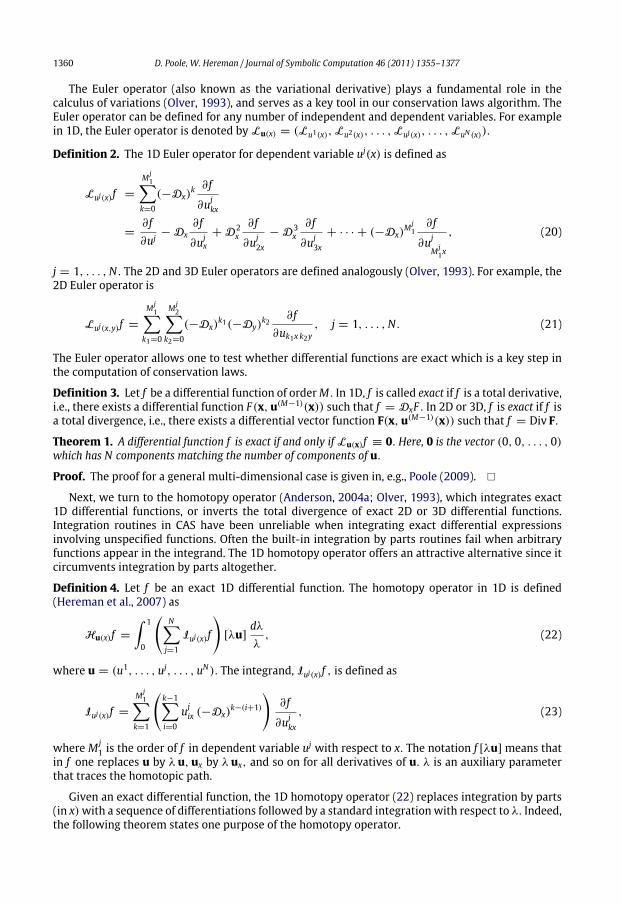
The Euler operator (also known as the variational derivative) plays a fundamental role in thecalculus of variations (Olver, 1993), and serves as a key tool in our conservation laws algorithm. TheEuler operator can be defined for any number of independent and dependent variables. For examplein 1D, the Euler operator is denoted by Lu(x) = (Lu1(x), Lu2(x), . . . , Luj(x), . . . , LuN (x)).
Definition 2. The 1D Euler operator for dependent variable uj(x) is defined as
Luj(x)f =
M j1−
k=0
(−Dx)k ∂ f
∂ujkx
=∂ f∂uj
− Dx∂ f
∂ujx
+ D2x
∂ f
∂uj2x
− D3x
∂ f
∂uj3x
+ · · · + (−Dx)M j
1∂ f
∂uj
M j1x
, (20)
j = 1, . . . ,N. The 2D and 3D Euler operators are defined analogously (Olver, 1993). For example, the2D Euler operator is
Luj(x,y)f =
M j1−
k1=0
M j2−
k2=0
(−Dx)k1(−Dy)
k2∂ f
∂uk1x k2y, j = 1, . . . ,N. (21)
The Euler operator allows one to test whether differential functions are exact which is a key step inthe computation of conservation laws.
Definition 3. Let f be a differential function of orderM. In 1D, f is called exact if f is a total derivative,i.e., there exists a differential function F(x,u(M−1)(x)) such that f = DxF . In 2D or 3D, f is exact if f isa total divergence, i.e., there exists a differential vector function F(x,u(M−1)(x)) such that f = Div F.
Theorem 1. A differential function f is exact if and only if Lu(x)f ≡ 0. Here, 0 is the vector (0, 0, . . . , 0)which has N components matching the number of components of u.
Proof. The proof for a general multi-dimensional case is given in, e.g., Poole (2009). �
Next, we turn to the homotopy operator (Anderson, 2004a; Olver, 1993), which integrates exact1D differential functions, or inverts the total divergence of exact 2D or 3D differential functions.Integration routines in CAS have been unreliable when integrating exact differential expressionsinvolving unspecified functions. Often the built-in integration by parts routines fail when arbitraryfunctions appear in the integrand. The 1D homotopy operator offers an attractive alternative since itcircumvents integration by parts altogether.
Definition 4. Let f be an exact 1D differential function. The homotopy operator in 1D is defined(Hereman et al., 2007) as
Hu(x)f =
∫ 1
0
N−j=1
Iuj(x)f
[λu]
dλλ
, (22)
where u = (u1, . . . , uj, . . . , uN). The integrand, Iuj(x)f , is defined as
Iuj(x)f =
M j1−
k=1
k−1−i=0
ujix (−Dx)
k−(i+1)
∂ f
∂ujkx
, (23)
where M j1 is the order of f in dependent variable uj with respect to x. The notation f [λu] means that
in f one replaces u by λu,ux by λux, and so on for all derivatives of u. λ is an auxiliary parameterthat traces the homotopic path.
Given an exact differential function, the 1D homotopy operator (22) replaces integration by parts(in x)with a sequence of differentiations followed by a standard integrationwith respect to λ. Indeed,the following theorem states one purpose of the homotopy operator.
D. Poole, W. Hereman / Journal of Symbolic Computation 46 (2011) 1355–1377 1361
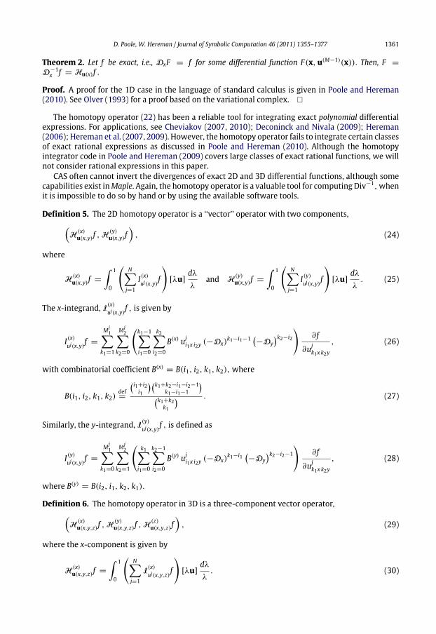
Theorem 2. Let f be exact, i.e., DxF = f for some differential function F(x,u(M−1)(x)). Then, F =
D−1x f = Hu(x)f .
Proof. A proof for the 1D case in the language of standard calculus is given in Poole and Hereman(2010). See Olver (1993) for a proof based on the variational complex. �
The homotopy operator (22) has been a reliable tool for integrating exact polynomial differentialexpressions. For applications, see Cheviakov (2007, 2010); Deconinck and Nivala (2009); Hereman(2006); Hereman et al. (2007, 2009). However, the homotopy operator fails to integrate certain classesof exact rational expressions as discussed in Poole and Hereman (2010). Although the homotopyintegrator code in Poole and Hereman (2009) covers large classes of exact rational functions, we willnot consider rational expressions in this paper.
CAS often cannot invert the divergences of exact 2D and 3D differential functions, although somecapabilities exist inMaple. Again, the homotopy operator is a valuable tool for computing Div−1,whenit is impossible to do so by hand or by using the available software tools.
Definition 5. The 2D homotopy operator is a ‘‘vector’’ operator with two components,H
(x)u(x,y)f , H
(y)u(x,y)f
, (24)
where
H(x)u(x,y)f =
∫ 1
0
N−j=1
I(x)uj(x,y)f
[λu]
dλλ
and H(y)u(x,y)f =
∫ 1
0
N−j=1
I(y)uj(x,y)f
[λu]
dλλ
. (25)
The x-integrand, I(x)uj(x,y)f , is given by
I(x)uj(x,y)f =
M j1−
k1=1
M j2−
k2=0
k1−1−i1=0
k2−i2=0
B(x) uji1x i2y (−Dx)
k1−i1−1 −Dy
k2−i2
∂ f
∂ujk1x k2y
, (26)
with combinatorial coefficient B(x)= B(i1, i2, k1, k2), where
B(i1, i2, k1, k2)def=
i1+i2i1
k1+k2−i1−i2−1k1−i1−1
k1+k2k1
. (27)
Similarly, the y-integrand, I(y)uj(x,y)f , is defined as
I(y)uj(x,y)f =
M j1−
k1=0
M j2−
k2=1
k1−
i1=0
k2−1−i2=0
B(y) uji1x i2y (−Dx)
k1−i1−Dy
k2−i2−1
∂ f
∂ujk1x k2y
, (28)
where B(y)= B(i2, i1, k2, k1).
Definition 6. The homotopy operator in 3D is a three-component vector operator,H
(x)u(x,y,z)f , H
(y)u(x,y,z)f , H
(z)u(x,y,z)f
, (29)
where the x-component is given by
H(x)u(x,y,z)f =
∫ 1
0
N−j=1
I(x)uj(x,y,z)f
[λu]
dλλ
. (30)
1362 D. Poole, W. Hereman / Journal of Symbolic Computation 46 (2011) 1355–1377
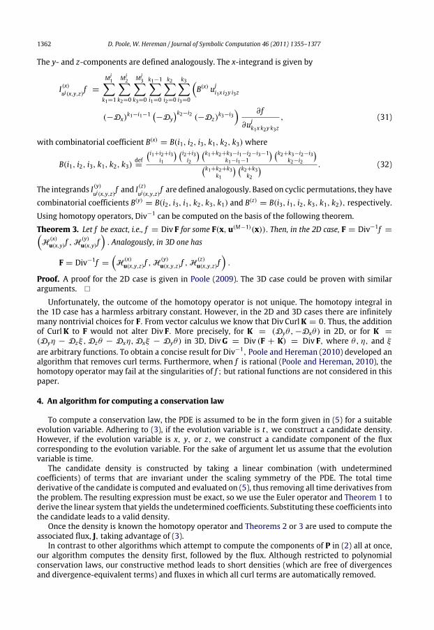
The y- and z-components are defined analogously. The x-integrand is given by
I(x)uj(x,y,z)f =
M j1−
k1=1
M j2−
k2=0
M j3−
k3=0
k1−1−i1=0
k2−i2=0
k3−i3=0
B(x) uj
i1x i2y i3z
(−Dx)k1−i1−1
−Dyk2−i2 (−Dz)
k3−i3 ∂ f
∂ujk1x k2y k3z
, (31)
with combinatorial coefficient B(x)= B(i1, i2, i3, k1, k2, k3) where
B(i1, i2, i3, k1, k2, k3)def=
i1+i2+i3i1
i2+i3i2
k1+k2+k3−i1−i2−i3−1k1−i1−1
k2+k3−i2−i3k2−i2
k1+k2+k3k1
k2+k3k2
. (32)
The integrands I(y)uj(x,y,z)f and I(z)uj(x,y,z)f are defined analogously. Based on cyclic permutations, they have
combinatorial coefficients B(y)= B(i2, i3, i1, k2, k3, k1) and B(z)
= B(i3, i1, i2, k3, k1, k2), respectively.
Using homotopy operators, Div−1 can be computed on the basis of the following theorem.
Theorem 3. Let f be exact, i.e., f = Div F for some F(x,u(M−1)(x)). Then, in the 2D case, F = Div−1f =H
(x)u(x,y)f , H
(y)u(x,y)f
. Analogously, in 3D one has
F = Div−1f =
H
(x)u(x,y,z)f , H
(y)u(x,y,z)f , H
(z)u(x,y,z)f
.
Proof. A proof for the 2D case is given in Poole (2009). The 3D case could be proven with similararguments. �
Unfortunately, the outcome of the homotopy operator is not unique. The homotopy integral inthe 1D case has a harmless arbitrary constant. However, in the 2D and 3D cases there are infinitelymany nontrivial choices for F. From vector calculus we know that Div CurlK = 0. Thus, the additionof CurlK to F would not alter Div F. More precisely, for K = (Dyθ, −Dxθ) in 2D, or for K =
(Dyη − Dzξ, Dzθ − Dxη, Dxξ − Dyθ) in 3D, DivG = Div (F + K) = Div F, where θ, η, and ξ
are arbitrary functions. To obtain a concise result for Div−1, Poole and Hereman (2010) developed analgorithm that removes curl terms. Furthermore, when f is rational (Poole and Hereman, 2010), thehomotopy operator may fail at the singularities of f ; but rational functions are not considered in thispaper.
4. An algorithm for computing a conservation law
To compute a conservation law, the PDE is assumed to be in the form given in (5) for a suitableevolution variable. Adhering to (3), if the evolution variable is t, we construct a candidate density.However, if the evolution variable is x, y, or z, we construct a candidate component of the fluxcorresponding to the evolution variable. For the sake of argument let us assume that the evolutionvariable is time.
The candidate density is constructed by taking a linear combination (with undeterminedcoefficients) of terms that are invariant under the scaling symmetry of the PDE. The total timederivative of the candidate is computed and evaluated on (5), thus removing all time derivatives fromthe problem. The resulting expression must be exact, so we use the Euler operator and Theorem 1 toderive the linear system that yields the undetermined coefficients. Substituting these coefficients intothe candidate leads to a valid density.
Once the density is known the homotopy operator and Theorems 2 or 3 are used to compute theassociated flux, J, taking advantage of (3).
In contrast to other algorithms which attempt to compute the components of P in (2) all at once,our algorithm computes the density first, followed by the flux. Although restricted to polynomialconservation laws, our constructive method leads to short densities (which are free of divergencesand divergence-equivalent terms) and fluxes in which all curl terms are automatically removed.
D. Poole, W. Hereman / Journal of Symbolic Computation 46 (2011) 1355–1377 1363
Definition 7. A term or expression f is a divergence if there exists a vector F such that f = Div F. In the1D case, f is a total derivative if there exists a function F such that f = DxF .Note thatDxf is essentiallya one-dimensional divergence. So, fromhere onwards, the term ‘‘divergence’’ will also cover the ‘‘totalderivative" case. Two ormore terms are divergence-equivalentwhen a linear combination of the termsis a divergence.
To illustrate the subtleties of the algorithm we intersperse the steps of the algorithm with twoexamples, viz., the ZK and KP equations.
4.1. Computing the scaling symmetry
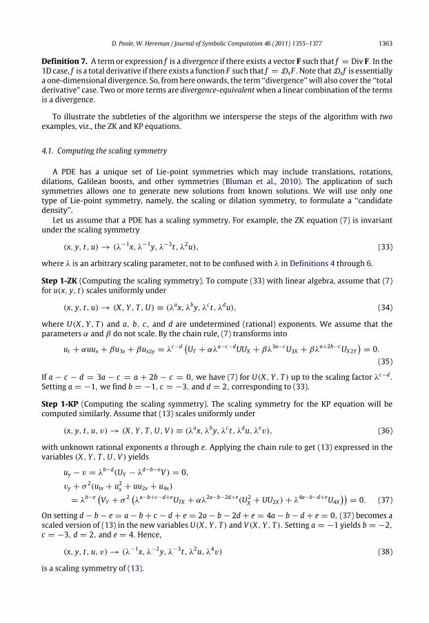
A PDE has a unique set of Lie-point symmetries which may include translations, rotations,dilations, Galilean boosts, and other symmetries (Bluman et al., 2010). The application of suchsymmetries allows one to generate new solutions from known solutions. We will use only onetype of Lie-point symmetry, namely, the scaling or dilation symmetry, to formulate a ‘‘candidatedensity’’.
Let us assume that a PDE has a scaling symmetry. For example, the ZK equation (7) is invariantunder the scaling symmetry
(x, y, t, u) → (λ−1x, λ−1y, λ−3t, λ2u), (33)
where λ is an arbitrary scaling parameter, not to be confused with λ in Definitions 4 through 6.
Step 1-ZK (Computing the scaling symmetry). To compute (33) with linear algebra, assume that (7)for u(x, y, t) scales uniformly under
(x, y, t, u) → (X, Y , T ,U) ≡ (λax, λby, λc t, λdu), (34)
where U(X, Y , T ) and a, b, c, and d are undetermined (rational) exponents. We assume that theparameters α and β do not scale. By the chain rule, (7) transforms into
ut + αuux + βu3x + βux2y = λc−d UT + αλa−c−dUUX + βλ3a−cU3X + βλa+2b−cUX2Y
= 0.(35)
If a − c − d = 3a − c = a + 2b − c = 0, we have (7) for U(X, Y , T ) up to the scaling factor λc−d.Setting a = −1, we find b = −1, c = −3, and d = 2, corresponding to (33).
Step 1-KP (Computing the scaling symmetry). The scaling symmetry for the KP equation will becomputed similarly. Assume that (13) scales uniformly under
(x, y, t, u, v) → (X, Y , T ,U, V ) ≡ (λax, λby, λc t, λdu, λev), (36)
with unknown rational exponents a through e. Applying the chain rule to get (13) expressed in thevariables (X, Y , T ,U, V ) yields
uy − v = λb−d(UY − λd−b−eV ) = 0,
vy + σ 2(utx + u2x + uu2x + u4x)
= λb−e VY + σ 2 λa−b+c−d+eUTX + αλ2a−b−2d+e(U2X + UU2X ) + λ4a−b−d+eU4X
= 0. (37)
On setting d − b − e = a − b + c − d + e = 2a − b − 2d + e = 4a − b − d + e = 0, (37) becomes ascaled version of (13) in the new variables U(X, Y , T ) and V (X, Y , T ). Setting a = −1 yields b = −2,c = −3, d = 2, and e = 4. Hence,
(x, y, t, u, v) → (λ−1x, λ−2y, λ−3t, λ2u, λ4v) (38)
is a scaling symmetry of (13).

1364 D. Poole, W. Hereman / Journal of Symbolic Computation 46 (2011) 1355–1377
4.2. Constructing a candidate component
Conservation law (2) must hold on solutions of the PDE. Therefore, we search for polynomialconservation laws that obey the scaling symmetry of the PDE. Indeed,we have yet to find a polynomialconservation law that does not adhere to the scaling symmetry.
On the basis of the scaling symmetry of the PDE, we choose a scaling factor for one of thecomponents of P in (2). The selected scaling factor will be called the rank (R) of that component.Then, we construct a candidate for that component as a linear combination of monomial terms (all ofrank R) with undetermined coefficients. By dynamically removing divergence terms and divergence-equivalent terms we make that candidate short and of low order.
Step 2-ZK (Building the candidate component). Since the ZK equation (7) has t as evolution variable,we will compute the density ρ of (3) of a fixed rank, for example, R = 6.
(a) Construct a list,P , of differential terms containing all powers of dependent variables and productsof dependent variables that have rank 6 or less. By (33), u has a scaling factor of 2, so u3 scales to rank6 and u2 has rank 4. This leads to P = {u3, u2, u}.
(b) Bring all of the terms in P up to rank 6 and put them into a new list, Q. This is done by applyingthe total derivative operators with respect to the space variables. Taking the terms in P , u3 has rank6 and is placed directly into Q. The term u2 has rank 4 and can be brought up to rank 6 in three ways:either by applying Dx twice, by applying Dy twice, or by applying each of Dx and Dy once, since bothDx andDy have scaling factors of 1. All three possibilities are considered and the resulting terms areput into Q. Similarly, the term u can be brought up to rank 6 in five ways, and all results are placedinto Q. Doing so,
Q = {u3, u2x , uu2x, u2
y, uu2y, uxuy, uuxy, u4x, u3xy, u2x2y, ux3y, u4y}, (39)
in which all monomials are now of rank 6.
(c)With the goal of constructing a nontrivial densitywith the least number of terms, remove all termsthat are divergences or are divergence-equivalent to other terms in Q. This can be done algorithmicallyby applying the Euler operator (21) to each term in (39), yielding
Lu(x,y)Q = {3u2, −2u2x, 2u2x, −2u2y, 2u2y, −2uxy, 2uxy, 0, 0, 0, 0, 0}. (40)
By Theorem 1, divergences are terms corresponding to 0 in (40). Hence, u4x, u3xy, u2x2y, ux3y, and u4yare divergences and can be removed from Q. Next, all divergence-equivalent terms will be removed.Following Hereman et al. (2005), form a linear combination of the terms that remained in (40) withundetermined coefficients pi, gathering like terms, and set it identically equal to zero,
3p1u2+ 2(p3 − p2)u2x + 2(p5 − p4)u2y + 2(p7 − p6)uxy = 0. (41)
Hence, p1 = 0, p2 = p3, p4 = p5, and p6 = p7. Terms with coefficients p3, p5, and p7 are divergence-equivalent to the terms with coefficients p2. p4, and p6, respectively. For each divergence-equivalentpair, the terms of highest order are removed from Q in (39). After all divergences and divergence-equivalent terms are removed, Q = {u3, u2
x , u2y, uxuy}.
(d) A candidate density is obtained by forming a linear combination of the remaining terms inQ usingundetermined coefficients ci. Thus, the candidate density of rank 6 for (7) is
ρ = c1u3+ c2u2
x + c3u2y + c4uxuy. (42)
Now,we turn to the KP equation (12). The conservation laws for the KP equation, (15) and (16), involvean arbitrary functional coefficient f (t). The scaling factor for f (t) depends on the degree if f (t) ispolynomial; whereas there is no scaling factor if f (t) is non-polynomial. In general, working withundetermined functional (instead of constant) coefficients f (x, y, z, t) would require a sophisticatedsolver for PDEs for f (seeWolf (2002)). Therefore, we cannot automatically compute (15) and (16) withour method. However, our algorithm can find conservation laws with explicit variable coefficients,e.g., tx2, txy, etc., as long as the degree is specified. Allowing such coefficients causes the candidate
D. Poole, W. Hereman / Journal of Symbolic Computation 46 (2011) 1355–1377 1365
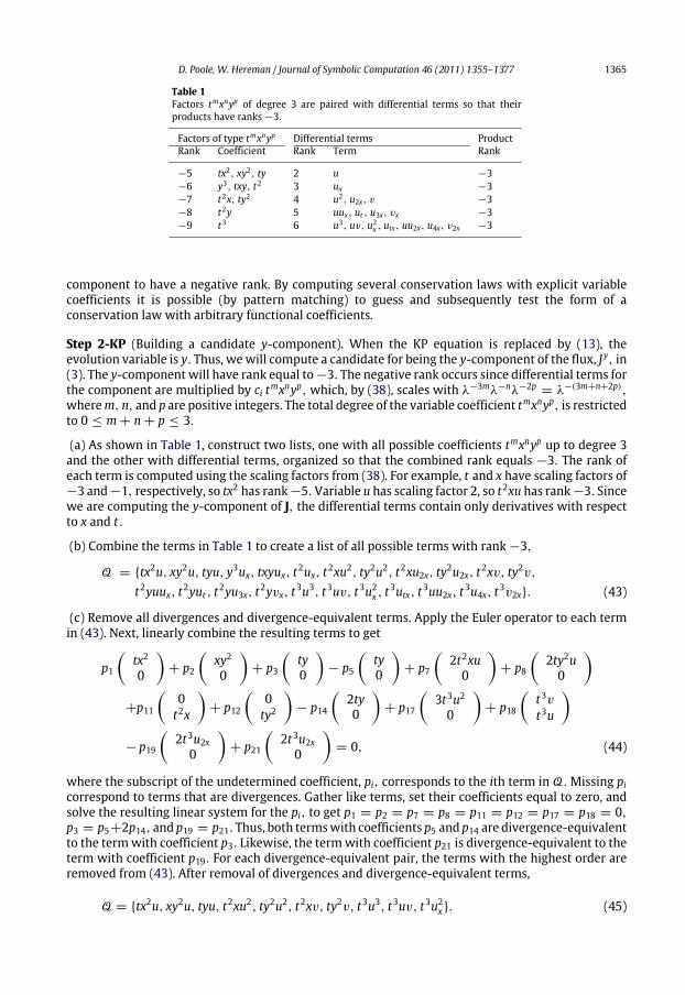
Table 1Factors tmxnyp of degree 3 are paired with differential terms so that theirproducts have ranks −3.
Factors of type tmxnyp Differential terms ProductRank Coefficient Rank Term Rank
−5 tx2, xy2, ty 2 u −3−6 y3, txy, t2 3 ux −3−7 t2x, ty2 4 u2, u2x, v −3−8 t2y 5 uux, ut , u3x, vx −3−9 t3 6 u3, uv, u2
x , utx, uu2x, u4x, v2x −3
component to have a negative rank. By computing several conservation laws with explicit variablecoefficients it is possible (by pattern matching) to guess and subsequently test the form of aconservation law with arbitrary functional coefficients.
Step 2-KP (Building a candidate y-component). When the KP equation is replaced by (13), theevolution variable is y. Thus, wewill compute a candidate for being the y-component of the flux, Jy, in(3). The y-component will have rank equal to−3. The negative rank occurs since differential terms forthe component are multiplied by ci tmxnyp, which, by (38), scales with λ−3mλ−nλ−2p
= λ−(3m+n+2p),wherem, n, and p are positive integers. The total degree of the variable coefficient tmxnyp, is restrictedto 0 ≤ m + n + p ≤ 3.
(a) As shown in Table 1, construct two lists, one with all possible coefficients tmxnyp up to degree 3and the other with differential terms, organized so that the combined rank equals −3. The rank ofeach term is computed using the scaling factors from (38). For example, t and x have scaling factors of−3 and−1, respectively, so tx2 has rank−5.Variable u has scaling factor 2, so t2xu has rank−3. Sincewe are computing the y-component of J, the differential terms contain only derivatives with respectto x and t.
(b) Combine the terms in Table 1 to create a list of all possible terms with rank −3,
Q = {tx2u, xy2u, tyu, y3ux, txyux, t2ux, t2xu2, ty2u2, t2xu2x, ty2u2x, t2xv, ty2v,
t2yuux, t2yut , t2yu3x, t2yvx, t3u3, t3uv, t3u2x , t
3utx, t3uu2x, t3u4x, t3v2x}. (43)
(c) Remove all divergences and divergence-equivalent terms. Apply the Euler operator to each termin (43). Next, linearly combine the resulting terms to get
p1
tx20
+ p2
xy20
+ p3
ty0
− p5
ty0
+ p7
2t2xu0
+ p8
2ty2u0
+p11
0t2x
+ p12
0ty2
− p14
2ty0
+ p17
3t3u2
0
+ p18
t3vt3u
− p19
2t3u2x
0
+ p21
2t3u2x
0
= 0, (44)
where the subscript of the undetermined coefficient, pi, corresponds to the ith term in Q. Missing picorrespond to terms that are divergences. Gather like terms, set their coefficients equal to zero, andsolve the resulting linear system for the pi, to get p1 = p2 = p7 = p8 = p11 = p12 = p17 = p18 = 0,p3 = p5+2p14, and p19 = p21. Thus, both termswith coefficients p5 and p14 are divergence-equivalentto the termwith coefficient p3. Likewise, the termwith coefficient p21 is divergence-equivalent to theterm with coefficient p19. For each divergence-equivalent pair, the terms with the highest order areremoved from (43). After removal of divergences and divergence-equivalent terms,
Q = {tx2u, xy2u, tyu, t2xu2, ty2u2, t2xv, ty2v, t3u3, t3uv, t3u2x}. (45)
1366 D. Poole, W. Hereman / Journal of Symbolic Computation 46 (2011) 1355–1377
(d) A linear combination of the terms in (45) with undetermined coefficients ci yields the candidate(of rank −3) for being the y-component of the flux, i.e.,
Jy = c1tx2u + c2xy2u + c3tyu + c4t2xu2+ c5ty2u2
+ c6t2xv+ c7ty2v + c8t3u3
+ c9t3uv + c10t3u2x . (46)
4.3. Evaluating the undetermined coefficients
All, part, or none of the candidate density (42) may be an actual density for the ZK equation. It isalso possible that the candidate is a linear combination of two ormore independent densities, yieldingindependent conservation laws. The true nature of the density will be revealed by computing theundetermined coefficients. By (3), Dtρ = −Div (Jx, Jy), so Dtρ must be a divergence with respectto the space variables x and y. Using Theorem 1, an algorithm for computing the undeterminedcoefficients readily follows.
Step 3-ZK (Computing the undetermined coefficients). To compute the undetermined coefficients,we form a system of linear equations for these coefficients. As part of the solution process, we alsogenerate compatibility conditions for the constant parameters in the PDE, if present.
(a) Compute the total derivative with respect to t of (42),
Dtρ = 3c1u2ut + 2c2uxutx + 2c3uyuty + c4(utxuy + uxuty). (47)
Let E = −Dtρ after ut and utx have been replaced using (7). This yields
E = 3c1u2(αuux + β(u3x + ux2y)) + 2c2ux(αuux + β(u3x + ux2y))x
+ 2c3uy(αuux + β(u3x + ux2y))y + c4(uy(αuux + β(u3x + ux2y))x
+ ux(αuux + β(u3x + ux2y))y). (48)
(b) By (3), E = Div (Jx, Jy). Therefore, by Theorem 1, Lu(x,y) E ≡ 0. Apply the Euler operator to (48),gather like terms, and set the result identically equal to zero:
0 ≡ Lu(x,y) E = −2(3c1β + c3α)uxu2y + 2(3c1β + c3α)uyuxy
+ 2c4αuxuxy + c4αuyu2x + 3(3c1β + c2α)uxu2x. (49)
(c) Form a linear system of equations for the undetermined coefficients ci by setting each coefficientequal to zero, thus satisfying (49). After eliminating duplicate equations, the system is
3c1β + c3α = 0, c4α = 0, 3c1β + c2α = 0. (50)
(d) Check for possible compatibility conditions on the parameters α and β in (50). This is done bysetting each ci = 1, one at a time, and algebraically eliminating the other undetermined coefficients.Consult Göktaş and Hereman (1997) for details about searching for compatibility conditions. System(50) is compatible for all nonzero α and β.
(e) Solve (50), taking into account the compatibility conditions (if applicable). Here,
c2 = c3 = −3β
αc1, c4 = 0, (51)
where c1 is arbitrary. We set c1 = 1 so that the density is normalized on the highest degree term,yielding
ρ = u3− 3
β
α(u2
x + u2y). (52)
Step 3-KP (Computing the undetermined coefficients). The procedure for finding the undeterminedcoefficients in the KP case is similar to that for the ZK case.
D. Poole, W. Hereman / Journal of Symbolic Computation 46 (2011) 1355–1377 1367
(a) Starting from (46), compute
DyJy = (c1x + 2c4tu)txuy + c2xy(2u + yuy) + (c3t + 2c5tyu)(u + yuy)
+ c6t2xvy + c7ty(2v + yvy) + 3c8t3u2uy + c9t3(uyv + uvy) + 2c10t3uxuxy, (53)
and replace uy and vy and their differential consequences using (13). Thus,
E = −DyJy = −(c1x + 2c4tu)txv − c2xy(2u + yv) − (c3t + 2c5tyu)(u + yv)
+ σ 2(c6t2x + c7ty2 + c9t3u)(utx + αu2x + αuu2x + u4x) − 2c7tyv
− 3c8t3u2v − c9t3v2− 2c10t3uxvx. (54)
(b) Apply the Euler operator to (54) and set the result identically equal to zero. This yields
(0, 0) = 0 ≡ Lu(t,x) E =Lu(t,x) E, Lv(t,x) E
= −
2c2xy + (c3 − 2σ 2c6)t + 2c4t2xv + 2c5ty(2u + yv) + 6c8t3uv
− 2σ 2c9t232ux + tutx + αtu2
x + αuu2x + tu4x
− 2c10t3v2x, c1tx2 + c2xy2
+ (c3 + 2c7)ty + 2c4t2xu + 2c5ty2u + 3c8t3u2+ 2c9t3v − 2c10t3u2x
. (55)
(c) Form a linear system for the undetermined coefficients ci. After duplicate equations and commonfactors have been removed, one gets
c1 = 0, c2 = 0, c3 − 2σ 2c6 = 0, c3 + 2c7 = 0, c4 = 0, c5 = 0,c8 = 0, c9 = 0, c10 = 0. (56)
(d) Compute potential compatibility conditions on the parameters α and σ . Again, the system iscompatible for all nonzero values of α and σ .
(e) Use σ 2= ±1 and solve the linear system, yielding
c1 = c2 = c4 = c5 = c8 = c9 = c10 = 0, c6 =12σ 2c3, c7 = −
12c3. (57)
Set c3 = −2 (to normalize the density) and substitute the result into (46), to obtain
Jy = −t(2yu + (σ 2tx − y2)v), (58)
which matches Jy in (15) if f (t) = t2 and v = uy.
4.4. Completing the conservation law
With the density (or a component of the flux at hand), the remaining components of theconservation law can be computed with the homotopy operator using Theorem 2 or 3.
Step 4-ZK (Computing the flux, J). Again, by the continuity equation (3), Div J = Div (Jx, Jy) =
−Dtρ = E. Therefore, compute Div−1 E, where the divergence is with respect to x and y. Aftersubstitution of (51) with c1 = 1 into (48),
E = 3u2(αuux + βu3x + βux2y) − 6β
αux(αuux + βu3x + βux2y)x
− 6β
αuy(αuux + βu3x + βux2y)y. (59)

1368 D. Poole, W. Hereman / Journal of Symbolic Computation 46 (2011) 1355–1377
Apply the 2D homotopy operator from Theorem 3. Compute the integrands (26) and (28):
I(x)u(x,y)E = 3αu4+ β
9u2
u2x +
23u2y
− 6u(3u2
x + u2y)
+
β2
α
6u2
2x + 5u2xy +
32u22y
+32u(u2x2y + u4y) − ux(12u3x + 7ux2y) − uy(3u3y + 8u2xy) +
52u2xu2y
, (60)
I(y)u(x,y)E = 3βu(uuxy − 4uxuy) −12
β2
α
3u(u3xy + ux3y) + ux(13u2xy + 3u3y)
+ 5uy(u3x + 3ux2y) − 9uxy(u2x + u2y), (61)
respectively. Use (25), to compute J =
H
(x)u(x,y)E, H
(y)u(x,y)E
where
H(x)u(x,y)E =
∫ 1
0
I
(x)u(x,y)E
[λu]
dλλ
=34αu4
+ β
3u2
u2x +
23u2y
− 2u(3u2
x + u2y)
+
β2
α
3u2
2x +52u2xy +
34u22y
+34u(u2x2y + u4y) − ux
6u3x +
72ux2y
− uy
32u3y + 4u2xy
+
54u2xu2y
, (62)
H(y)u(x,y)E =
∫ 1
0
I
(x)u(x,y)E
[λu]
dλλ
= βu(uuxy − 4uxuy) −14
β2
α
3u(u3xy + ux3y) + ux(13u2xy + 3u3y)
+ 5uy(u3x + 3ux2y) − 9uxy(u2x + u2y). (63)
Notice that J has a curl term, K = (Dyθ, −Dxθ), with
θ = 2βu2uy +14
β2
α
3u(u2xy + u3y) + 5(2uxuxy + 3uyu2y + u2xuy)
. (64)
Therefore, compute J − K to obtain
Jx = 3u214αu2
+ βu2x
− 2βu(u2
x + u2y) +
β2
α(u2
2x − u22y)
− 2β2
α(ux(u3x + ux2y) + uy(u2xy + u3y))
, (65)
Jy = 3βu2uxy + 2
β
αuxy(u2x + u2y)
, (66)
which match the components in (10).
Step 4-KP (Computing the density and the x-component of the flux). For the KP example, (ρ, Jx)remains to be computed. Using the continuity equation (3), Dtρ + DxJx = −DyJy = E. Thus, tofind (ρ, Jx), compute Div−1E, where this time the divergence is with respect to t and x. Proceed as inthe previous example. First, substitute (57) and c3 = −2 into (54),
E = t2u +
σ 2y2 − tx
(utx + αu2
x + αuu2x + u4x). (67)
Second, compute the integrands for the homotopy operator,
I(t)u(t,x)E = −12(uDx − uxI)
∂E∂utx
=12t(tu + (σ 2y2 − tx)ux), (68)
D. Poole, W. Hereman / Journal of Symbolic Computation 46 (2011) 1355–1377 1369
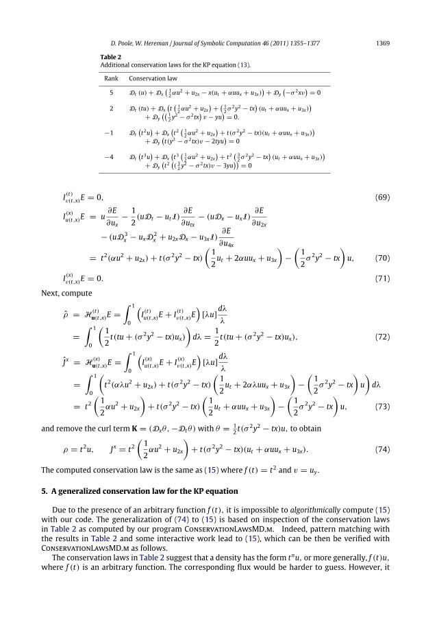
Table 2Additional conservation laws for the KP equation (13).
Rank Conservation law
5 Dt (u) + Dx 12αu2
+ u2x − x(ut + αuux + u3x)+ Dy
−σ 2xv
= 0
2 Dt (tu) + Dxt 12αu2
+ u2x+ 12σ 2y2 − tx
(ut + αuux + u3x)
+ Dy
12 y
2− σ 2tx
v − yu
= 0.
−1 Dtt2u+ Dx
t2 12αu2
+ u2x+ t(σ 2y2 − tx)(ut + αuux + u3x)
+ Dy
t(y2 − σ 2tx)v − 2tyu
= 0
−4 Dtt3u+ Dx
t3 12αu2
+ u2x+ t2
32σ 2y2 − tx
(ut + αuux + u3x)
+ Dy
t2( 32 y
2− σ 2tx)v − 3yu
= 0
I(t)v(t,x)E = 0, (69)
I(x)u(t,x)E = u∂E∂ux
−12(uDt − utI)
∂E∂utx
− (uDx − uxI)∂E
∂u2x
− (uD3x − uxD
2x + u2xDx − u3xI)
∂E∂u4x
= t2(αu2+ u2x) + t(σ 2y2 − tx)
12ut + 2αuux + u3x
−
12σ 2y2 − tx
u, (70)
I(x)v(t,x)E = 0. (71)
Next, compute
ρ = H(t)u(t,x)E =
∫ 1
0
I(t)u(t,x)E + I(t)v(t,x)E
[λu]
dλλ
=
∫ 1
0
12t(tu + (σ 2y2 − tx)ux)
dλ =
12t(tu + (σ 2y2 − tx)ux), (72)
Jx = H(x)u(t,x)E =
∫ 1
0
I(x)u(t,x)E + I(x)v(t,x)E
[λu]
dλλ
=
∫ 1
0
t2(αλu2
+ u2x) + t(σ 2y2 − tx)12ut + 2αλuux + u3x
−
12σ 2y2 − tx
udλ
= t212αu2
+ u2x
+ t(σ 2y2 − tx)
12ut + αuux + u3x
−
12σ 2y2 − tx
u, (73)
and remove the curl term K = (Dxθ, −Dtθ) with θ =12 t(σ
2y2 − tx)u, to obtain
ρ = t2u, Jx = t212αu2
+ u2x
+ t(σ 2y2 − tx)(ut + αuux + u3x). (74)
The computed conservation law is the same as (15) where f (t) = t2 and v = uy.
5. A generalized conservation law for the KP equation
Due to the presence of an arbitrary function f (t), it is impossible to algorithmically compute (15)with our code. The generalization of (74) to (15) is based on inspection of the conservation lawsin Table 2 as computed by our program ConservationLawsMD.m. Indeed, pattern matching withthe results in Table 2 and some interactive work lead to (15), which can be then be verified withConservationLawsMD.m as follows.
The conservation laws in Table 2 suggest that a density has the form tnu, or more generally, f (t)u,where f (t) is an arbitrary function. The corresponding flux would be harder to guess. However, it
1370 D. Poole, W. Hereman / Journal of Symbolic Computation 46 (2011) 1355–1377
can be computed as follows. Since the KP equation (13) is an evolution equation in y, we construct asuitable candidate for being Jy. Guided by the results in Table 2, we take
Jy = c1f ′(t)yu + c2f ′(t)y2v + c3f (t)xv, (75)
where c1, c2, and c3 are undetermined coefficients, and uy is replaced by v in agreement with (13). Asbefore, we compute DyJy and replace uy and vy using (13). Doing so,
E = DyPy= c1f ′u + (c1 + 2c2)f ′yv − (σ 2c2f ′y2 + σ 2c3fx)(utx + αu2
x + αuu2x + u4x). (76)
By (3), DyJy = −Div(ρ, Jx). By Theorem 1,
(0, 0) = 0 ≡ Lu(t,x)E =(c1 − σ 2c3)f ′, (c1 + 2c2)f ′y
. (77)
Clearly, c2 = −12 c1 and c3 = σ 2c1. If we set c1 = −1 and v = uy we obtain Jy in (15). Application
of the homotopy operator (in this case to an expression with arbitrary functional coefficients) yields(ρ, Jx). This is how conservation law (15) was computed. Conservation law (16) was obtained in asimilar way. Both conservation laws were then verified using the ConservationLawsMD.m code.
6. Applications
In this sectionwe state results obtained by using our algorithm on a variety of (2+1)- and (3+1)-dimensional nonlinear PDEs. The selected PDEs highlight several of the issues that arise when usingour algorithm and software package ConservationLawsMD.m.
6.1. The Sawada–Kotera Equation in 2D
The (2+1)-dimensional SK equation (Konopelchenko and Dubrovsky, 1984),
ut = 5u2ux + 5uu3x + 5uuy + 5uxu2x + 5u2xy + u5x − 5∂−1x u2y + 5ux∂
−1x uy, (78)
with u(x) = u(x, y, t) is a completely integrable 2D generalization of the standard SK equation. Thelatter has infinitely many conservation laws (see, e.g., Göktaş and Hereman (1997)). Our algorithmcannot handle the integral terms in (78), so we set v = ∂−1
x uy. Doing so, (78) becomes a system ofevolution equations in y:
vy = −15ut + u2ux + uu3x + uvx + uxu2x + v3x +
15u5x + uxv, uy = vx. (79)
Application of our algorithm to (79) yields several conservation laws, all of which have densitiesu, tu, t2u, etc., and yu, tyu, t2yu, etc. Like with the KP equation, this suggests that there areconservation laws with an arbitrary functional coefficient f (t). Proceeding as in Section 5 and usingConservationLawsMD.m, we obtained
Dt (fu) + Dx
f ′yv − 5f
13u3
+ uv + uu2x + uxy +15u4x
+ Dy
5f v − f ′yu
= 0, (80)
Dt (fyu) + Dx
12f ′y2 − 5fx
v − 5fy
13u3
+ uv + uu2x + uxy +15u4x
+ Dy
5fyv −
12f ′y2 − 5fx
u
= 0. (81)
Note that the densities in (80) and (81) are identical to those in (15) and (16) for the KP equation.These two densities occur often in (2 + 1)-dimensional PDEs that have a utx instead of a ut term, asshown in the next example.
D. Poole, W. Hereman / Journal of Symbolic Computation 46 (2011) 1355–1377 1371
6.2. The Khokhlov–Zabolotskaya equation in 2D and 3D
TheKhokhlov–Zabolotskaya (KZ) equation or dispersionless KP equation describes the propagationof sound in nonlinearmedia in two or three space dimensions (Sanders andWang, 1997a). The (2+1)-dimensional KZ equation,
(ut − uux)x − u2y = 0, (82)
with u(x) = u(x, y, t) can be written as a system of evolution equations in y,
uy = v, vy = utx − u2x − uu2x, (83)
by setting v = uy. Again, two familiar densities appear in the following conservation laws, computedindirectly as we showed for the KP and SK equations:
Dt(ux) + Dx(−uux) + Dy(−uy) = 0, (84)
Dt (fu) + Dx
−
12fu2
−
12f ′y2 + fx
(ut − uux)
+ Dy
12f ′y2 + fx
uy − f ′yu
= 0, (85)
Dt (fyu) + Dx
−
12fyu2
− y16f ′y2 + fx
(ut − uux)
+ Dy
y16f ′y2 + fx
uy −
12f ′y2 + fx
u
= 0, (86)
where f (t) is an arbitrary function. Actually, (85) and (86) are nonlocal because, from (82), ut − uux =u2y dx. By swapping terms in the density and the x-component of the flux, (85), with f (t) = 1, can
be rewritten as
Dt (xux) + Dx
12u2
− xuux
+ Dy
−xuy
= 0, (87)
which is local. The computation of conservation laws for the (3 + 1)-dimensional KZ equation,
(ut − uux)x − u2y − u2z = 0, (88)
where u(x) = u(x, y, z, t), is more difficult. This equation can be written as a system of evolutionequations in either y or z. Although the intermediate results differ, either choice leads to equivalentconservation laws. Writing (88) as an evolution system in z,
uz = v, vz = utx − u2x − uu2x − u2y, (89)
ConservationLawsMD.m is able to compute a variety of conservation lawswhose densities are shownin Table 3.
Density ρ1 = xux in Table 3 is part of local conservation law
Dt (xux) + Dx
12u2
− xuux
+ Dy
−xuy
+ Dz (−xuz) = 0, (90)
which can be rewritten as a nonlocal conservation law
Dt (u) + Dx
−
12u2
− x(ut − uux)
+ Dy
xuy+ Dz (xuz) = 0. (91)
In general, if a factor xux appears in a density then that factor can be replaced by u. Doing so, alldensities in Table 3 that can be expressed as ρ = g(y, z, t)u, where g(y, z, t) is arbitrary. Introducing
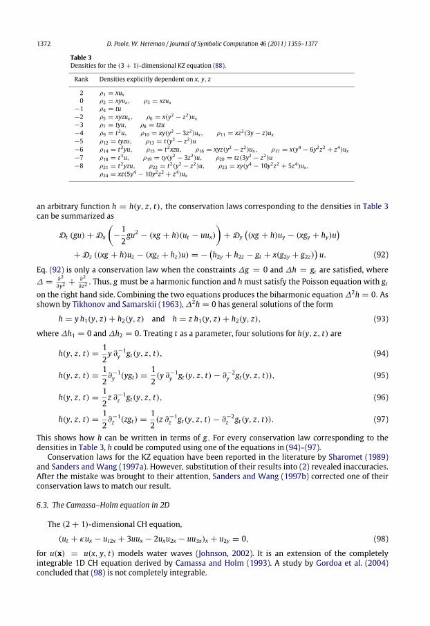
1372 D. Poole, W. Hereman / Journal of Symbolic Computation 46 (2011) 1355–1377
Table 3Densities for the (3 + 1)-dimensional KZ equation (88).
Rank Densities explicitly dependent on x, y, z
2 ρ1 = xux0 ρ2 = xyux, ρ3 = xzux
−1 ρ4 = tu−2 ρ5 = xyzux, ρ6 = x(y2 − z2)ux−3 ρ7 = tyu, ρ8 = tzu−4 ρ9 = t2u, ρ10 = xy(y2 − 3z2)ux, ρ11 = xz2(3y − z)ux−5 ρ12 = tyzu, ρ13 = t(y2 − z2)u−6 ρ14 = t2yu, ρ15 = t2xzu, ρ16 = xyz(y2 − z2)ux, ρ17 = x(y4 − 6y2z2 + z4)ux−7 ρ18 = t3u, ρ19 = ty(y2 − 3z2)u, ρ20 = tz(3y2 − z2)u−8 ρ21 = t2yzu, ρ22 = t2(y2 − z2)u, ρ23 = xy(y4 − 10y2z2 + 5z4)ux,
ρ24 = xz(5y4 − 10y2z2 + z4)ux
an arbitrary function h = h(y, z, t), the conservation laws corresponding to the densities in Table 3can be summarized as
Dt (gu) + Dx
−
12gu2
− (xg + h)(ut − uux)
+ Dy
(xg + h)uy − (xgy + hy)u
+ Dz ((xg + h)uz − (xgz + hz)u) = −
h2y + h2z − gt + x(g2y + g2z)
u. (92)
Eq. (92) is only a conservation law when the constraints ∆g = 0 and ∆h = gt are satisfied, where∆ =
∂2
∂y2+
∂2
∂z2. Thus, g must be a harmonic function and h must satisfy the Poisson equation with gt
on the right hand side. Combining the two equations produces the biharmonic equation ∆2h = 0. Asshown by Tikhonov and Samarskii (1963), ∆2h = 0 has general solutions of the form
h = y h1(y, z) + h2(y, z) and h = z h1(y, z) + h2(y, z), (93)
where ∆h1 = 0 and ∆h2 = 0. Treating t as a parameter, four solutions for h(y, z, t) are
h(y, z, t) =12y ∂−1
y gt(y, z, t), (94)
h(y, z, t) =12∂−1y (ygt) =
12(y ∂−1
y gt(y, z, t) − ∂−2y gt(y, z, t)), (95)
h(y, z, t) =12z ∂−1
z gt(y, z, t), (96)
h(y, z, t) =12∂−1z (zgt) =
12(z ∂−1
z gt(y, z, t) − ∂−2z gt(y, z, t)). (97)
This shows how h can be written in terms of g. For every conservation law corresponding to thedensities in Table 3, h could be computed using one of the equations in (94)–(97).
Conservation laws for the KZ equation have been reported in the literature by Sharomet (1989)and Sanders and Wang (1997a). However, substitution of their results into (2) revealed inaccuracies.After the mistake was brought to their attention, Sanders and Wang (1997b) corrected one of theirconservation laws to match our result.
6.3. The Camassa–Holm equation in 2D
The (2 + 1)-dimensional CH equation,
(ut + κux − ut2x + 3uux − 2uxu2x − uu3x)x + u2y = 0, (98)
for u(x) = u(x, y, t) models water waves (Johnson, 2002). It is an extension of the completelyintegrable 1D CH equation derived by Camassa and Holm (1993). A study by Gordoa et al. (2004)concluded that (98) is not completely integrable.
D. Poole, W. Hereman / Journal of Symbolic Computation 46 (2011) 1355–1377 1373
Obviously, (98) is a conservation law itself,
Dt(ux − u3x) + Dx(κux + 3uux − 2uxu2x − uu3x) + Dy(uy) = 0. (99)
It can be written as a system of evolution equations in y. Indeed,
uy = v, vy = −(αut + κux − ut2x + 3βuux − 2uxu2x − uu3x)x. (100)
Note that we introduced auxiliary parameters α and β as coefficients of the ut and uux terms,respectively. The reason for doing so is that the CH equation (98) does not have a scaling symmetryunless we add scales on the parameters α, β and κ. Our code guided us in finding the followingconservation laws with functional coefficients:
Dt (fu) + Dx
1αf32βu2
+ κu −12u2x − uu2x − utx
+
12f ′y2 −
1αfx
(αut + κux
+ 3βuux − 2uxu2x − uu3x − ut2x
+ Dy
12f ′y2 −
1αfxuy − f ′yu
= 0, (101)
Dt (fyu) + Dx
1αfy32βu2
+ κu −12u2x − uu2x − utx
+ y
16f ′y2 −
1αfx
× (αut + κux + 3βuux − 2uxu2x − uu3x − ut2x)
+ Dy
y16f ′y2 −
1αfxuy
+
1αfx −
12f ′y2
u
= 0, (102)
where f (t) is arbitrary and without constraints on the parameters. Thus, if we set α = β = 1, wehave conservation laws for (98).
6.4. The Gardner equation in 2D
The (2 + 1)-dimensional Gardner equation (Konopelchenko and Dubrovsky, 1984),
ut = −32α2u2ux + 6βuux + u3x − 3αux∂
−1x uy + 3∂−1
x u2y, (103)
for u(x) = u(x, y, t) is a 2D generalization of
ut = −32αu2ux + 6βuux + u3x, (104)
which is an integrable combination of the KdV and mKdV equations due to Gardner. For α = 0, (103)reduces to the KP equation (12). For β = 0, (103) becomes a modified KP equation. Adding a newdependent variable, v = ∂−1
x uy, allows one to remove the integral terms and replace (103) by thesystem
uy = vx, vy =13ut −
13u3x − 2βuux + αuxv +
12α2u2ux. (105)
For (103), we found two conservation laws with constant coefficients,
Dt (u) + Dx
12α2u3
− 3βu2+ 3αuv − u2x
+ Dy
−
32αu2
+ 3v
= 0, (106)
Dtu2
+ Dx
34α2u4
− 4βu3+ 3αu2v + 3v2
+ u2x − 2uu2x
+ Dy
−u(αu2
+ 6v)
= 0. (107)
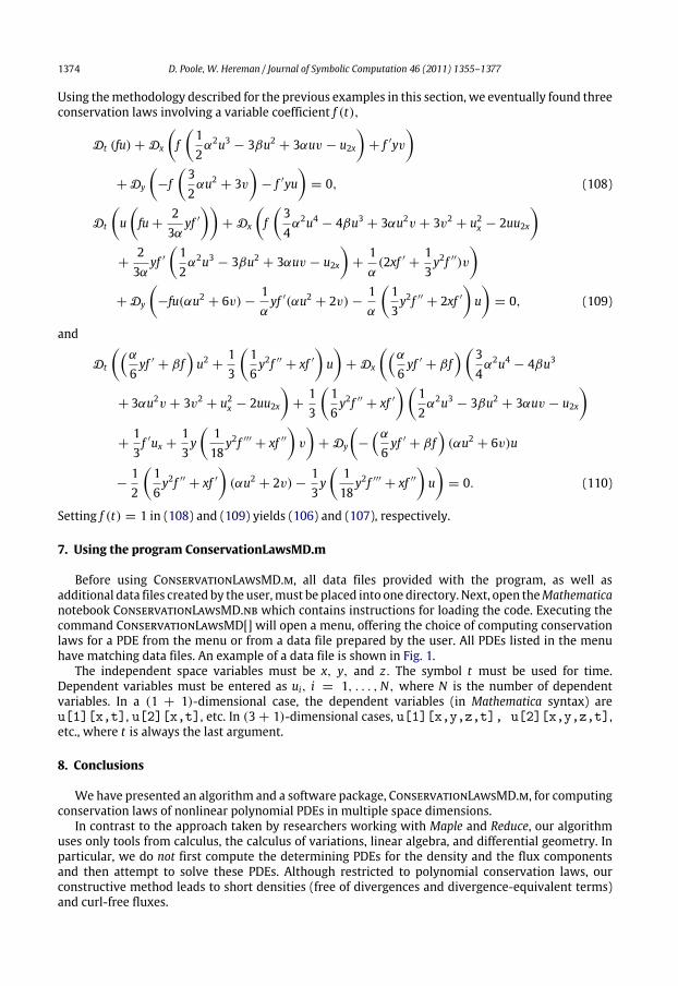
1374 D. Poole, W. Hereman / Journal of Symbolic Computation 46 (2011) 1355–1377
Using themethodology described for the previous examples in this section, we eventually found threeconservation laws involving a variable coefficient f (t),
Dt (fu) + Dx
f12α2u3
− 3βu2+ 3αuv − u2x
+ f ′yv
+ Dy
−f32αu2
+ 3v
− f ′yu
= 0, (108)
Dt
ufu +
23α
yf ′
+ Dx
f34α2u4
− 4βu3+ 3αu2v + 3v2
+ u2x − 2uu2x
+
23α
yf ′
12α2u3
− 3βu2+ 3αuv − u2x
+
1α
(2xf ′+
13y2f ′′)v
+ Dy
−fu(αu2
+ 6v) −1αyf ′(αu2
+ 2v) −1α
13y2f ′′
+ 2xf ′
u
= 0, (109)
and
Dt
α
6yf ′
+ βfu2
+13
16y2f ′′
+ xf ′
u
+ Dx
α
6yf ′
+ βf3
4α2u4
− 4βu3
+ 3αu2v + 3v2+ u2
x − 2uu2x
+
13
16y2f ′′
+ xf ′
12α2u3
− 3βu2+ 3αuv − u2x
+
13f ′ux +
13y
118
y2f ′′′+ xf ′′
v
+ Dy
−
α
6yf ′
+ βf
(αu2+ 6v)u
−12
16y2f ′′
+ xf ′
(αu2
+ 2v) −13y
118
y2f ′′′+ xf ′′
u
= 0. (110)
Setting f (t) = 1 in (108) and (109) yields (106) and (107), respectively.
7. Using the program ConservationLawsMD.m
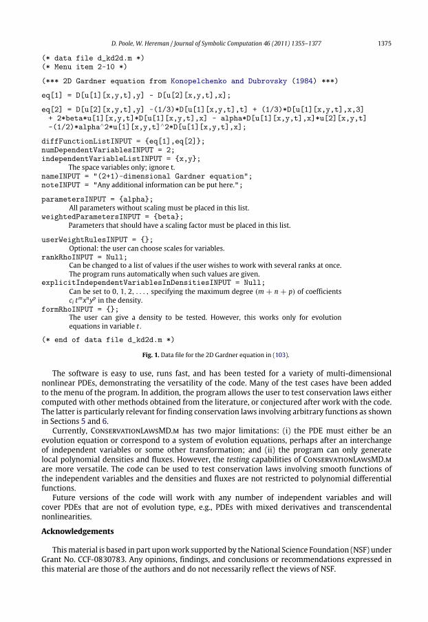
Before using ConservationLawsMD.m, all data files provided with the program, as well asadditional data files created by the user,must be placed into one directory. Next, open theMathematicanotebook ConservationLawsMD.nb which contains instructions for loading the code. Executing thecommand ConservationLawsMD[] will open a menu, offering the choice of computing conservationlaws for a PDE from the menu or from a data file prepared by the user. All PDEs listed in the menuhave matching data files. An example of a data file is shown in Fig. 1.
The independent space variables must be x, y, and z. The symbol t must be used for time.Dependent variables must be entered as ui, i = 1, . . . ,N, where N is the number of dependentvariables. In a (1 + 1)-dimensional case, the dependent variables (in Mathematica syntax) areu[1][x,t], u[2][x,t], etc. In (3 + 1)-dimensional cases, u[1][x,y,z,t], u[2][x,y,z,t],etc., where t is always the last argument.
8. Conclusions
Wehave presented an algorithm and a software package, ConservationLawsMD.m, for computingconservation laws of nonlinear polynomial PDEs in multiple space dimensions.
In contrast to the approach taken by researchers working with Maple and Reduce, our algorithmuses only tools from calculus, the calculus of variations, linear algebra, and differential geometry. Inparticular, we do not first compute the determining PDEs for the density and the flux componentsand then attempt to solve these PDEs. Although restricted to polynomial conservation laws, ourconstructive method leads to short densities (free of divergences and divergence-equivalent terms)and curl-free fluxes.
D. Poole, W. Hereman / Journal of Symbolic Computation 46 (2011) 1355–1377 1375
(* data file d_kd2d.m *)(* Menu item 2-10 *)
(*** 2D Gardner equation from Konopelchenko and Dubrovsky (1984) ***)
eq[1] = D[u[1][x,y,t],y] - D[u[2][x,y,t],x];
eq[2] = D[u[2][x,y,t],y] -(1/3)*D[u[1][x,y,t],t] + (1/3)*D[u[1][x,y,t],x,3]+ 2*beta*u[1][x,y,t]*D[u[1][x,y,t],x] - alpha*D[u[1][x,y,t],x]*u[2][x,y,t]-(1/2)*alpha∧2*u[1][x,y,t]∧2*D[u[1][x,y,t],x];
diffFunctionListINPUT = {eq[1],eq[2]};numDependentVariablesINPUT = 2;independentVariableListINPUT = {x,y};
The space variables only; ignore t.nameINPUT = "(2+1)-dimensional Gardner equation";noteINPUT = "Any additional information can be put here.";
parametersINPUT = {alpha};All parameters without scaling must be placed in this list.
weightedParametersINPUT = {beta};Parameters that should have a scaling factor must be placed in this list.
userWeightRulesINPUT = {};Optional: the user can choose scales for variables.
rankRhoINPUT = Null;Can be changed to a list of values if the user wishes to work with several ranks at once.The program runs automatically when such values are given.
explicitIndependentVariablesInDensitiesINPUT = Null;Can be set to 0, 1, 2, . . . , specifying the maximum degree (m + n + p) of coefficientsci tmxnyp in the density.
formRhoINPUT = {};The user can give a density to be tested. However, this works only for evolutionequations in variable t.
(* end of data file d_kd2d.m *)
Fig. 1. Data file for the 2D Gardner equation in (103).
The software is easy to use, runs fast, and has been tested for a variety of multi-dimensionalnonlinear PDEs, demonstrating the versatility of the code. Many of the test cases have been addedto the menu of the program. In addition, the program allows the user to test conservation laws eithercomputed with other methods obtained from the literature, or conjectured after work with the code.The latter is particularly relevant for finding conservation laws involving arbitrary functions as shownin Sections 5 and 6.
Currently, ConservationLawsMD.m has two major limitations: (i) the PDE must either be anevolution equation or correspond to a system of evolution equations, perhaps after an interchangeof independent variables or some other transformation; and (ii) the program can only generatelocal polynomial densities and fluxes. However, the testing capabilities of ConservationLawsMD.mare more versatile. The code can be used to test conservation laws involving smooth functions ofthe independent variables and the densities and fluxes are not restricted to polynomial differentialfunctions.
Future versions of the code will work with any number of independent variables and willcover PDEs that are not of evolution type, e.g., PDEs with mixed derivatives and transcendentalnonlinearities.
Acknowledgements
Thismaterial is based in part uponwork supported by theNational Science Foundation (NSF) underGrant No. CCF-0830783. Any opinions, findings, and conclusions or recommendations expressed inthis material are those of the authors and do not necessarily reflect the views of NSF.

1376 D. Poole, W. Hereman / Journal of Symbolic Computation 46 (2011) 1355–1377
Mark Hickman (University of Canterbury, Christchurch, New Zealand) and Bernard Deconinck(University of Washington, Seattle) are gratefully acknowledged for valuable discussions. Undergrad-uate students Jacob Rezac, John-Bosco Tran, and Travis ‘‘Alan" Volz are thanked for their helpwith thisproject. We thank the anonymous referees whose constructive comments and suggestions helped usto further improve the manuscript.
References
Ablowitz, M.J., Clarkson, P.A., 1991. Solitons, Nonlinear Evolution Equations and Inverse Scattering. Cambridge University Press,Cambridge, UK.
Ablowitz, M.A., Segur, H., 1981. Solitons and the Inverse Scattering Transform. In: SIAM Stud. in Appl. Math., vol. 4. SIAM,Philadelphia, Pennsylvania.
Anderson, I.M., 2004a. The Variational Complex. Dept. of Mathematics, Utah State University, Logan, Utah, 318 pages.Manuscript available at http://www.math.usu.edu/~fg_mp/Publications/VB/vb.pdf.
Anderson, I.M., 2004b. The Vessiot package; the software with documentation is available at http://www.math.usu.edu/∼fg_mp/Pages/SymbolicsPage/VessiotDownloads.html.
Anderson, I.M., Cheb-Terrab, E., 2009. DifferentialGeometry package, Maple Online Help, www.maplesoft.com/support/help/Maple/view.aspx?path=DifferentialGeometry.
Baldwin, D., Hereman, W., 2010. A symbolic algorithm for computing recursion operators of nonlinear PDEs. Int. J. Comput.Math. 87, 1094–1119.
Bluman, G.W., Cheviakov, A.F., Anco, S.C., 2010. Applications of Symmetry Methods to Partial Differential Equations. In: Appl.Math. Sciences, vol. 168. Springer-Verlag, New York.
Camassa, R., Holm, D.D., 1993. An integrable shallow water equation with peaked solutions. Phys. Rev. Lett. 71, 1661–1664.Cheb-Terrab, E., von Bulow, K., 2004. PDEtools package, Maple Online Help, http://www.maplesoft.com/support/help/Maple/
view.aspx?path=PDEtools.Cheviakov, A.F., 2007. GeM software package for computation of symmetries and conservation laws of differential equations.
Comput. Phys. Comm. 76, 48–61.Cheviakov, A.F., 2010. Computation of fluxes of conservation laws. J. Engrg. Math. 66, 153–173.Deconinck, B., Nivala, M., 2009. Symbolic integration and summation using homotopy operators. Math. Comput. Simulation 80,
825–836.Drinfel’d, V.G., Sokolov, V.V., 1985. Lie algebras and equations of Korteweg–de Vries type. J. Sov. Math. 30, 1975–2036.Göktaş, Ü., Hereman, W., 1997. Symbolic computation of conserved densities for systems of nonlinear evolution equations.
J. Symbolic Comput. 24, 591–621.Gordoa, P.G., Pickering, A., Senthilvelan,M., 2004. Evidence for thenonintegrability of awaterwave equation in 2+1dimensions.
Zeit. für Naturfor. 59a, 640–644.Hereman,W., 2006. Symbolic computation of conservation laws of nonlinear partial differential equations inmulti-dimensions.
Int. J. Quantum Chem. 106, 278–299.Hereman, W., Adams, P.J., Eklund, H.L., Hickman, M.S., Herbst, B.M., 2009. Direct methods and symbolic software for
conservation laws of nonlinear equations. In: Yan, Z. (Ed.), Advances in Nonlinear Waves and Symbolic Computation. NovaScience Publishers, New York, pp. 19–79.
Hereman, W., Colagrosso, M., Sayers, R., Ringler, A., Deconinck, B., Nivala, M., Hickman, M.S., 2005. Continuous and discretehomotopy operators and the computation of conservation laws. In: Wang, D., Zheng, Z. (Eds.), Differential Equations withSymbolic Computation. Birkhäuser, Basel, pp. 249–285.
Hereman, W., Deconinck, B., Poole, L.D., 2007. Continuous and discrete homotopy operators: a theoretical approach madeconcrete. Math. Comput. Simulation 74, 352–360.
Infeld, E., 1985. Self-focusing nonlinear waves. J. Plasma Phys. 33, 171–182.Johnson, R.S., 2002. Camassa–Holm, Korteweg–de Vries and related models for water waves. J. Fluid Mech. 455, 63–82.Kadomtsev, B.B., Petviashvili, V.I., 1970. On the stability of solitary waves in weakly dispersive media. Sov. Phys. Dokl. 15,
539–541.Konopelchenko, B.G., Dubrovsky, V.G., 1984. Some new integrable nonlinear evolution equations in 2 + 1 dimensions. Phys.
Lett. A 102, 15–17.Lax, P.D., 1968. Integrals of nonlinear equations of evolution and solitary waves. Commun. Pure Appl. Math. 21, 467–490.Miura, R.M., Gardner, C.S., Kruskal, M.D., 1968. Korteweg–de Vries equation and generalizations II. Existence of conservation
laws and constants of motion. J. Math. Phys. 9, 1204–1209.Naz, R., 2008. Symmetry solutions and conservation laws for some partial differential equations in field mechanics, Ph.D.
dissertation, University of the Witwatersrand, Johannesburg.Naz, R.,Mahomed, F.M.,Mason, D.P., 2008. Comparison of different approaches to conservation laws for somepartial differential
equations in fluid mechanics. Appl. Math. Comput. 205, 212–230.Newell, A.C., 1983. The history of the soliton. J. Appl. Mech. 50, 1127–1138.Olver, P.J., 1993. Applications of Lie Groups to Differential Equations, 2nd ed.. In: Grad. Texts inMath., vol. 107. Springer-Verlag,
New York.Poole, L.D., 2009. Symbolic computation of conservation laws of nonlinear partial differential equations using homotopy
operators, Ph.D. dissertation, Colorado School of Mines, Golden, Colorado.Poole, D., Hereman, W., 2009. HomotopyIntegrator.m: a Mathematica package for the application of the homotopy method
for (i) integration by parts of expressions involving unspecified functions of one variable and (ii) the inversion of a totaldivergence involving unspecified functions of two or three independent variables; software available at http://inside.mines.edu/∼whereman under scientific software.
D. Poole, W. Hereman / Journal of Symbolic Computation 46 (2011) 1355–1377 1377
Poole, D., Hereman, W., 2009. ConservationLawsMD.m: a Mathematica package for the symbolic computation of conservationlaws of polynomial systems of nonlinear PDEs in multiple space dimensions, software available at http://inside.mines.edu/∼whereman under scientific software.
Poole, D., Hereman, W., 2010. The homotopy operator method for symbolic integration by parts and inversion of divergenceswith applications. Appl. Anal. 87, 433–455.
Rosenhaus, V., 2002. Infinite symmetries and conservation laws. J. Math. Phys. 43, 6129–6150.Sanders, J., Wang, J.P., 1997a. Hodge decomposition and conservation laws. Math. Comput. Simulation 44, 483–493.Sanders, J., Wang, J.P., 1997b. Hodge decomposition and conservation laws; corrected paper, see URL http://www.math.vu.nl/
∼jansa/#research.Sanz-Serna, J.M., 1982. An explicit finite-difference scheme with exact conservation properties. J. Comput. Phys. 47, 199–210.Sharomet, N.O., 1989. Symmetries, invariant solutions and conservation laws of the nonlinear acoustics equation. Acta Appl.
Math. 15, 83–120.Shivamoggi, B.K., Rollins, D.K., Fanjul, R., 1993. Analytic aspects of the Zakharov–Kuznetsov equation. Phys. Scr. 47, 15–17.Tikhonov, A.N., Samarskii, A.A., 1963. Equations of Mathematical Physics. Dover Publications, New York.Vinogradov, A.M., 1989. Symmetries and conservation laws of partial differential equations: basic notions and results. Acta
Appl. Math. 15, 3–21.Wolf, T., 2002. A comparison of four approaches to the calculation of conservation laws. European J. Appl. Math. 13, 129–152.Zakharov, V.E., Kuznetsov, E.A., 1974. Three-dimensional solitons. Sov. Phys. JETP 39, 285–286.Zakharov, V.E., Shabat, A.B., 1972. Exact theory of two-dimensional self-focusing and one-dimensional self-modulation ofwaves
in nonlinear media. Sov. Phys. JETP 34, 62–69.