Symbol approach in a signal-restoration problem

involving block Toeplitz matrices∗

Vincenza Del Prete †, Fabio Di Benedetto ‡, Marco Donatelli §, Stefano Serra-Capizzano ¶

August 3, 2014

Abstract

We consider a special type of signal restoration problem where some of the sampling data are notavailable. The formulation related to samples of the function and its derivative leads to a possiblylarge linear system associated to a nonsymmetric block Toeplitz matrix which can be equipped with a2 × 2 matrix-valued symbol. The aim of the paper is to study the eigenvalues of the matrix. We firstidentify in detail the symbol and its analytical features. Then, by using recent results on the eigenvaluedistribution of block Toeplitz matrix-sequences, we formally describe the cluster sets and the asymptoticspectral distribution of the matrix-sequences related to our problem. The localization areas, the extremalbehavior, and the conditioning are only observed numerically, but their behavior is strongly related tothe analytical properties of the symbol, even though a rigorous proof is still missing in the block case.

1 Introduction and description of the problem

We consider a special type of signal restoration problem, where a finite number of samples of a band limitedsignal is lost. A band limited signal is a function belonging to the space Bω of the square-integrable functions,whose Fourier transform is supported in [−ω, ω]. Functions belonging to this space can be represented by theShannon series, which is an expansion in terms of the orthonormal basis of translates of the sinc function.The coefficients of the expansion, called sampling formula, are the samples of the function at a uniform gridon R, with “density ω/π”(Nyquist density). This theory has been extended by replacing the orthonormalbasis with more general families, like Riesz bases or frames, formed by translates of a single or more functionsand other sampling formulae have been obtained (see the one-channel (4) and the two-channel (15) formulasand reference [1]). Frames, unlike Riesz or orthonormal bases, are overcomplete and their redundancy allowsthe recovery of missing samples.

The problem of the recovery of missing samples has been first investigated by Ferreira in [8] where theauthor shows that, under suitable oversampling assumptions, any finite set of samples can be recoveredfrom the others. The recovery technique uses an oversampling one-channel formula (see (4)) and consists insolving a structured linear system (I −S)X = B where S is a positive definite matrix, whose eigenvalues liein the interval (0, 1). If the missing samples are equidistant, this matrix is a scalar symmetric Toeplitz matrixassociated to a scalar symbol (a characteristic function); thus, by standard localization and by distributionresults [4], the eigenvalues lie in the convex hull of the symbol range and are clustered at the range.

∗This is a preprint of a paper published in J. Comput. Appl. Math., 272 (2014), pp. 399416.†Dipartimento di Matematica, Via Dodecaneso 35, 16146 Genova (ITALY) (E-mail: delprete@dima.unige.it)‡Dipartimento di Matematica, Via Dodecaneso 35, 16146 Genova (ITALY) (E-mail: dibenede@dima.unige.it)§Dipartimento di Scienza e alta Tecnologia, Via Valleggio 11, 22100 Como (ITALY) (E-mail:

marco.donatelli@uninsubria.it)¶Dipartimento di Scienza e alta Tecnologia, Via Valleggio 11, 22100 Como (ITALY) (E-mail:

stefano.serrac@uninsubria.it)

1

In a further step, Santos and Ferreira considered the case of the two-channel derivative oversamplingformula [10], in which a band limited function is expanded in terms of the translates of two functions(generators) (see (15)) and the coefficients are the samples of the function and its derivative. The authors of[10] show that a finite number of missing samples either of the function or of the derivative can be recovered,solving in each case a nonsingular linear system. Their technique extends in a natural way to the case wherethe missing samples come both from the function and its derivative, leading to a system (I − S)X = B,where the matrix S (see (19)) is a 2 × 2 block matrix depending on the generators and on the position ofthe missing samples. The unknowns X are the missing samples of the function and of its derivative.

In [1] Brianzi and Del Prete, using Ferreira’s technique, studied the stability of the matrix in the two-channel derivative case, especially when the missing samples are located in positions

U = {mi1,m i2, . . . ,m in},

where m is an integer (interleaving factor). The practical interest for studying these cases lies in thetechnique of interleaving the samples of a signal, prior to their transmission or archival; the advantage ofthis procedure is that the transmitted (or stored) information becomes less sensitive to the burst errorsthat typically affect contiguous set of samples [8]. The authors have obtained estimates of the minimumand maximum eigenvalues of the block submatrices of the matrix S, showing that in some cases the matrixreduces to a (block) lower triangular matrix. Moreover they performed several numerical experiments onthe dependence of the eigenvalues on the parameters of the problem and on the reconstruction of the signal,also in the ill-conditioned case of contiguous missing samples.

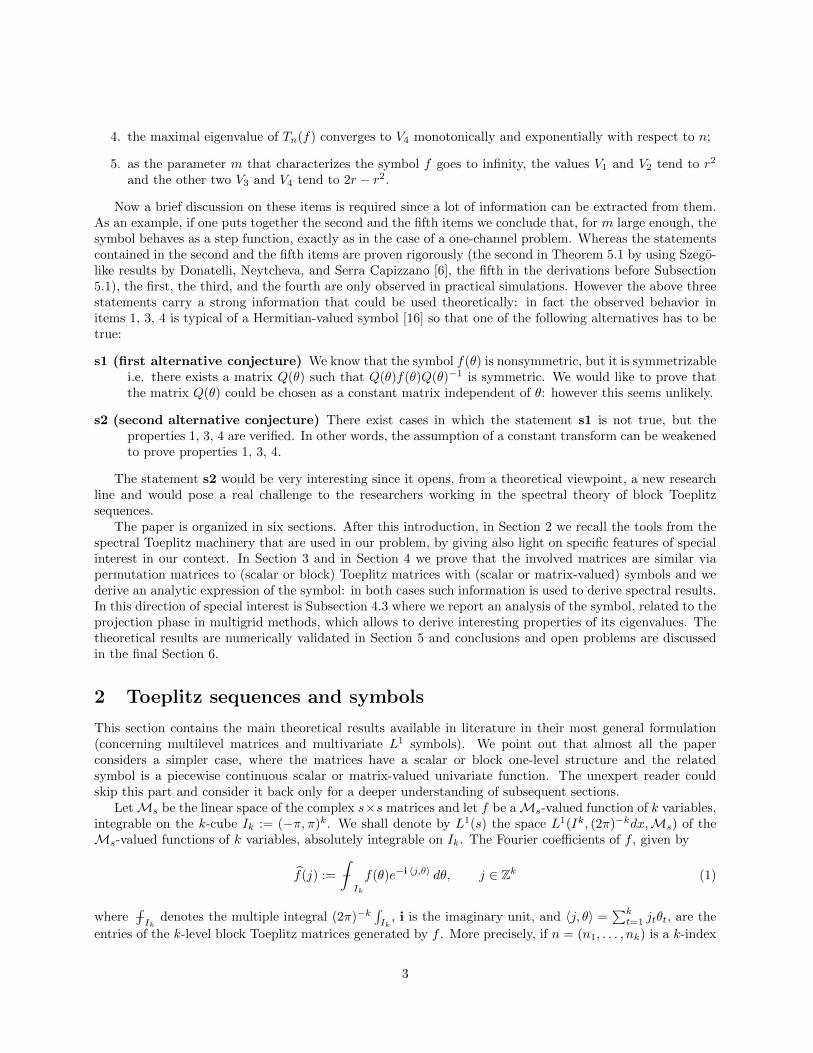
In this paper we consider the case of missing samples of the function and of its derivative at equidistantpoints. The formulation of the related signal restoration problem leads to a nonsymmetric block Toeplitzmatrix, possibly large. Here we perform three steps. First we construct an explicit expression of the symbolf , by interpreting the entries of the matrix as Fourier coefficients of the symbol. As a second step, we studythe related symbol and, as a third step, we use the information for giving a spectral characterization of thematrices S in terms of the different parameters. More specifically, concerning the second step, we provethat the double channel matrix is similar (via a permutation transform) to a standard block Toeplitz matrixTn(f) with 2-by-2 nonsymmetric matrix-valued symbol f(θ) associated with two main parameters: theoversampling parameter r ∈ (0, 1) (see (13)) and the interleaving factor m (positive integer), both dependingon the problem. For any choice of the parameters the eigenvalues λ1(f(θ)) and λ2(f(θ)) of f(θ) have thefollowing features:

(i) their range is real (proved formally),

(ii) their range consists of two intervals contained in (0, 1) (proved formally only for special sets of theparameters).

For specific choices of the parameters it can also be seen that the range of λ1(f(θ)) is made by two singlepoints V1, V2 and the range of λ2(f(θ)) is made by two single points V3, V4 with 0 < V1 ≤ V2 ≤ V3 ≤ V4 < 1and where the Lebesgue measure of the θ-values such that λ(f(θ)) = Vj is a positive number Mj for everyj = 1, 2, 3, 4. In addition this behavior of the symbol (though not proved rigorously for every possible choiceof the parameters) seems to be general. On the other hand, the numerical tests show that

1. all the eigenvalues of Tn(f) are contained in (V1, V4);

2. the global spectrum of the sequence {Tn(f)} is distributed as the symbol f (see Theorem 2.3 andTheorem 5.1) and it is clustered to the set {V1, V2, V3, V4} and the number of the eigenvalues which areclose within ε to Vj is equal to 2Mjn+o(n) (the quantity named o(n) seems to grow only logarithmicallywith n) where the Mj ’s are the Lebesgue measures mentioned above with M1 +M2 +M3 +M4 = 2πi.e. the total measure of the definition set of the symbol;

3. the minimal eigenvalue of Tn(f) converges to V1 monotonically and exponentially with respect to n;

2

4. the maximal eigenvalue of Tn(f) converges to V4 monotonically and exponentially with respect to n;

5. as the parameter m that characterizes the symbol f goes to infinity, the values V1 and V2 tend to r2

and the other two V3 and V4 tend to 2r − r2.

Now a brief discussion on these items is required since a lot of information can be extracted from them.As an example, if one puts together the second and the fifth items we conclude that, for m large enough, thesymbol behaves as a step function, exactly as in the case of a one-channel problem. Whereas the statementscontained in the second and the fifth items are proven rigorously (the second in Theorem 5.1 by using Szego-like results by Donatelli, Neytcheva, and Serra Capizzano [6], the fifth in the derivations before Subsection5.1), the first, the third, and the fourth are only observed in practical simulations. However the above threestatements carry a strong information that could be used theoretically: in fact the observed behavior initems 1, 3, 4 is typical of a Hermitian-valued symbol [16] so that one of the following alternatives has to betrue:

s1 (first alternative conjecture) We know that the symbol f(θ) is nonsymmetric, but it is symmetrizablei.e. there exists a matrix Q(θ) such that Q(θ)f(θ)Q(θ)−1 is symmetric. We would like to prove thatthe matrix Q(θ) could be chosen as a constant matrix independent of θ: however this seems unlikely.

s2 (second alternative conjecture) There exist cases in which the statement s1 is not true, but theproperties 1, 3, 4 are verified. In other words, the assumption of a constant transform can be weakenedto prove properties 1, 3, 4.

The statement s2 would be very interesting since it opens, from a theoretical viewpoint, a new researchline and would pose a real challenge to the researchers working in the spectral theory of block Toeplitzsequences.

The paper is organized in six sections. After this introduction, in Section 2 we recall the tools from thespectral Toeplitz machinery that are used in our problem, by giving also light on specific features of specialinterest in our context. In Section 3 and in Section 4 we prove that the involved matrices are similar viapermutation matrices to (scalar or block) Toeplitz matrices with (scalar or matrix-valued) symbols and wederive an analytic expression of the symbol: in both cases such information is used to derive spectral results.In this direction of special interest is Subsection 4.3 where we report an analysis of the symbol, related to theprojection phase in multigrid methods, which allows to derive interesting properties of its eigenvalues. Thetheoretical results are numerically validated in Section 5 and conclusions and open problems are discussedin the final Section 6.

2 Toeplitz sequences and symbols

This section contains the main theoretical results available in literature in their most general formulation(concerning multilevel matrices and multivariate L1 symbols). We point out that almost all the paperconsiders a simpler case, where the matrices have a scalar or block one-level structure and the relatedsymbol is a piecewise continuous scalar or matrix-valued univariate function. The unexpert reader couldskip this part and consider it back only for a deeper understanding of subsequent sections.

LetMs be the linear space of the complex s×s matrices and let f be aMs-valued function of k variables,integrable on the k-cube Ik := (−π, π)k. We shall denote by L1(s) the space L1(Ik, (2π)−kdx,Ms) of theMs-valued functions of k variables, absolutely integrable on Ik. The Fourier coefficients of f , given by

f(j) := −∫Ik

f(θ)e−i 〈j,θ〉 dθ, j ∈ Zk (1)

where −∫Ik

denotes the multiple integral (2π)−k∫Ik

, i is the imaginary unit, and 〈j, θ〉 =∑kt=1 jtθt, are the

entries of the k-level block Toeplitz matrices generated by f . More precisely, if n = (n1, . . . , nk) is a k-index

3

with positive entries, then Tn(f) denotes the matrix of order sn (throughout, we let n :=∏ki=1 ni) given by

Tn(f) =∑|j1|<n1

· · ·∑|jk|<nk

[J (j1)n1⊗ · · · ⊗ J (jk)

nk

]⊗ f(j1, . . . , jk). (2)

In this case, we say that the sequence {Tn(f)} is generated by the symbol f . In the above equation, ⊗ denotes

the tensor product, whereas J(l)t denotes the matrix of order t whose (i, j) entry equals 1 if j − i = l and

equals zero otherwise: the reader is referred to [18] for more details on multilevel block Toeplitz matrices.

2.1 Eigenvalue Localization for non-Hermitian block Toeplitz matrices

We first recall some localization results concerning singular values that turn out to be useful also to localizethe eigenvalues of block Toeplitz matrices. In the following, the considered measure µ{·} is the Lebesguemeasure on Rk for some integer k ≥ 1 and σmin(f) and σmax(f) denote the essential infimum and theessential supremum (with respect to the Lebesgue measure) of the singular values of f . Furthermore, if f isHermitian-valued then λmin(f) and λmax(f) denote the essential infimum and the essential supremum (withrespect to the Lebesgue measure) of the eigenvalues of f .

Definition 2.1 Suppose f ∈ L1(s). Assume that, for any x ∈ Ik, σj(f(θ))/λj(f(θ)) denotes the j-thsingular/eigen value of f(θ). Then the quantities σmin(f) and σmax(f) are defined as follows:

σmin(f) = sup {c ∈ R : µ{θ ∈ Ik : min1≤j≤sσj(f(θ)) < c} = 0}

and

σmax(f) = inf {C ∈ R : µ{θ ∈ Ik : max1≤j≤sσj(f(θ)) > C} = 0} .

Furthermore, if f is Hermitian-valued then the quantities λmin(f) and λmax(f) are defined as follows:

λmin(f) = sup {c ∈ R : µ{θ ∈ Ik : min1≤j≤sλj(f(θ)) < c} = 0}

and

λmax(f) = inf {C ∈ R : µ{θ ∈ Ik : max1≤j≤sλj(f(θ)) > C} = 0} .

Finally we introduce the notion of Essential Numerical Range (ENR(f)) of f which is the set of all thecomplex numbers y so that for any positive ε we have µ{x ∈ Ik : ∃v so that ‖v‖2 = 1 and v∗f(x)v ∈B(y, ε)} > 0 where B(y, ε) = {z ∈ C : |z − y| ≤ ε}.

If s = 1 (scalar case) then σmin(f) and σmax(f) coincide with the essential infimum and the essentialsupremum of |f |. Here the word “essential” means up to zero measure sets: in general, for the sake ofsimplicity, we will indicate inf h and suph instead of essinf h and esssup h for measurable functions h.Moreover in the case of s = 1, the quantity ENR(f) coincides with ER(f) i.e. with the standard essentialrange (for the notion of essential range of a scalar valued function see [9]). In the scalar case, the followingTheorem 2.1 is essentially already in [2].

Theorem 2.1 [15] Suppose f ∈ L1(s). Suppose also that there exists a straight line z in the complexplane such that, denoting by H1 and H2 the two open half-planes such that C = H1

⋃z⋃H2, it holds

ENR(f)⋂H1 = ∅ and 0 ∈ H1

⋃z. Let d(z) ≥ 0 denote the distance of z from the origin (generalization

of the notion of weakly sectoriality [15]). Then if σ is a singular value of Tn(f), it holds σ ≥ d. Inaddition if ω is the rotation number so that z = {w ∈ C : Rew = d} and if the minimal eigenvalue ofωf(θ) + ωf∗(θ) is not identically equal to d, then the inequality is strict that is σ > d. Finally, we havesupz∈S{d(z)} = maxz∈S{d(z)} = δ where S is the set of all separating lines and δ is defined as the distanceof the complex zero from the convex hull of ENR(f) (when s = 1 then the constant δ is the distance of thecomplex zero from Coh[ER(f)] where Coh[X] denotes the convex hull of a subset X of the complex plane).

4

Theorem 2.2 [15] Suppose f, g ∈ L1(s). Consider R(f, g) = {λ ∈ C : P(f − λg)} where the propositionP(h) is true if the function h, h ∈ L1(s), satisfies the assumptions of Theorem 2.1. Suppose also that P(g)holds. Then, for any n, the eigenvalues of T−1

n (g)Tn(f) belong to [R(f, g)]c i.e. to the complementary set ofR(f, g).

The assumptions of Theorem 2.1 are trivially satisfied when ENR(f) ⊂ R (it suffices to choose e.g.z = {w ∈ C : Imw = 0} and H1 = {w ∈ C : Imw > 0}), but this will not happen in the two-channelcase. However, consider the case g = I (the s × s identity matrix): except for pathological situations,ENR(f − λI) = ENR(f)− λ and therefore Theorem 2.2 says that λ is in a localization region for the spec-trum whenever a translation of ENR(f) by λ is not well separated from the origin (in the sense of Theorem2.1). In several cases, this means that the spectrum is localized in terms of the convex hull of ENR(f).

It is quite immediate to observe that the tools given in Theorem 2.1 and in Theorem 2.2 are difficult touse in pratice. The following observation gives a series of indications on how to use the results (especiallyin our setting).

Remark 2.1 In Theorem 2.2, if f is similar to f via a constant transformation and g is similar to g viathe same constant transformation, then T−1

n (g)Tn(f) is similar to T−1n (g)Tn(f) and therefore for any n, the

eigenvalues of T−1n (g)Tn(f) belong to [R(f , g)]c as well. As a consequence if F denotes the set of all the

pairs (f , g) satisfying the previous assumptions, then for any n, the eigenvalues of T−1n (g)Tn(f) belong to⋂

(f ,g)∈F [R(f , g)]c i.e. to the intersection of all complementary sets of R(f , g).We will be interested in the particular case where g = I and f is similar to a Hermitian-valued symbol

via a constant transform; then all the eigenvalues of Tn(f) are real and belong to the interval

[λmin(f), λmax(f)].

Furthermore, if min1≤j≤sλj(f(θ)) is not constantly equal to λmin(f), then the localization interval becomesopen on the left (λmin(f), λmax(f)]. Analogously, if max1≤j≤sλj(f(θ)) is not constantly equal to λmax(f),then the localization interval becomes open on the right [λmin(f), λmax(f)), so that if both min1≤j≤sλj(f(θ))and max1≤j≤sλj(f(θ)) are not constant the localization result is refined by replacing the closed interval withthe open interval

(λmin(f), λmax(f)).

As we will see this is the case occurring for the symbols appearing in the one-channel and two-channelproblems, even if there is theoretical gap since we have been not able to prove the existence of a constantsimilarity transform which makes the symbol Hermitian (see items s1, s2 and the related discussion in theIntroduction). As a final remark, if

µ{θ ∈ Ik : min1≤j≤sλj(f(θ)) = λmin(f)} > 0

then the monotone convergence (from above) of the minimal eigenvalue of Tn(f) to λmin(f) is exponentiallyfast; in perfect analogy, if

µ{θ ∈ Ik : max1≤j≤sλj(f(θ)) = λmax(f)} > 0

then the monotone convergence (from below) of the maximal eigenvalue of Tn(f) to λmax(f) is exponentiallyfast. It is worth stressing that the latter situation occurs, both for the minimal and the maximal eigenvaluesof Tn(f), for our one-channel and two-channel problems.

2.2 Asymptotic results for the spectrum of non-Hermitian block Toeplitz se-quences

Among the several asymptotic results for block Toeplitz sequences and their generalizations, we recall atheorem which is especially suited in our context since it gives the Szego formula and the cluster sets for thematrices coming from the one-channel and two-channel problems.

5

Theorem 2.3 [6] Let f ∈ L∞(s) with eigenvalues λj(f), j = 1, . . . , s, and let Λn be the spectrum of Tn(f).Define R(f) =

⋃sj=1R(λj(f)) as the union of the essential ranges of the eigenvalues of f . If R(f) has empty

interior part and does not disconnect the complex plane, then for every function F ∈ C0(C) continuous withbounded support, the following asymptotic formula

limn→∞

1

ns

∑λ∈Λn

F (λ) = −∫Ik

1

str(F (f(θ))) dθ (3)

holds. The latter relation is indicated in short using the notation {Tn(f)} ∼λ (f, Ik).

We emphasize that in our problems k = 1 and s = 1 (one-channel problem) or s = 2 (two-channelproblem). In both the cases the set R(f) is made by only qs real numbers in the interval (0, 1), at least fora wide choice of parameters, where q1 = 2 and q2 = 4. Therefore the assumptions of the above theorem aretrivially fulfilled and the distribution result holds so that {Tn(f)} ∼λ (f, I1).

We conclude this preliminary section of tools by giving a visual interpretation of the above distributionalTheorem 2.3: we focus our attention to the case where k = 1 and f(θ) is piecewise continuous as inthe application at hand. In fact, a practical reading of formula (3), for every test function F continuous

with bounded support, is that the eigenvalues of Tn(f) can be partitioned in s sets Λ(1)n , . . . ,Λ

(s)n , each of

cardinality n (since k = 1). A suitable ordering of the pairs(−π +

2πj

n, λ

(l)j

), j = 1, . . . , n, λ

(l)j ∈ Λ(l)

n ,

reconstructs, approximately for n large enough, the function

θ → λl(f(θ))

for every l = 1, . . . , s. In other words, the pairs(−π +

2πj

n, λ

(l)j

)≈(−π +

2πj

n, λl

(f

(−π +

2πj

n

)))are approximate sampling values of the function λl(f(θ)).

3 One-channel case: the symbol and the spectral analysis

First, we briefly summarize the general one-channel case and recall some stability results obtained in [8]. Inthe following we shall denote by χ[−T,T ] the characteristic function of the interval [−T, T ]. The Shannonone-channel oversampling formula for a signal F in Bω is

F(x) =ωt0π

∑n∈ZF(nt0)

sin(ω(x− nt0))

ω(x− nt0), (4)

where t0 is less then the Nyquist density π/ω. We shall denote by r the oversampling parameter

r =ωt0π.

Note that if r = 1, the family of the translates of the function

sinc(x) = sin(πx)/πx

becomes an orthonormal basis. Let U = {l1, l2, . . . , ln} be a set of integers and

{F(lkt0) : k = 1, . . . , n} (5)

6

be the set of missing samples. By evaluating (4) in lkt0, k = 1, . . . , n and separating the known samplesfrom the unknown ones, we obtain the following system

(I − S)X = B, (6)

where I is the identity n× n matrix,

S(j, k) = r sinc(r(lj − lk)), j, k = 1, . . . , n,

X = (F(lkt0))nk=1, B = (b1, b2, . . . , bn)T , and

bj = r∑k/∈U

F(kt0)sinc(r(lj − lk)), j = 1, . . . , n.

The matrix S is symmetric and positive definite. In [8], the author observes that when r is close to 1the recovery is impossible. This is in agreement with the theory, since for r = 1 the family of translatesof the sinc function is not a frame but an orthonormal basis and S is the identity matrix. In addition, theauthor shows that all its eigenvalues are in (0, 1) for every choice of the set U , by observing that S is alwaysa principal submatrix of a scalar Toeplitz prolate matrix of sufficiently large order. Recall that the n × nprolate matrix is defined as

M := (rsinc[r(j − k)])nj,k=1. (7)

An interesting situation occurs when U consists of equidistant points: let m be the interleaving factorand set U = {m, 2m, . . . , nm}. In this case the matrix S

S := (rsinc[r(j − k)m])nj,k=1 (8)

keeps the Toeplitz structure and it can be seen as a generalization of M . For instance, in [8] the quadraticforms associated to the matrices M and S are expressed as follows

v∗Mv =1

2

∫ r

−r|φ(t)|2 dt, v∗Sv =

1

2

∫ r

−r|φ(t)|2 dt, (9)

where v = (v1, v2, . . . vn)T , φ(t) =∑n−1k=0 vke

iπkt and φ(t) =∑n−1k=0 vke

iπmkt. Note that φ(t) = φ(mt).The prolate matrix M is studied in detail in [20] and is generated, in the sense of the previous section,

by a scalar symbol represented by the characteristic function χ[−rπ,rπ]. This fact is related to the identity

2w + 2

+∞∑k=1

sin 2kπw

kπcos kθ = χ[−2πw,2πw](θ), for |θ| 6= 2πw and w ∈ (0, 1/2) (10)

and to the integral expression in (9) for v∗Mv. Given the strong analogy with the formula associated to Sin (9), we are tempted to conclude that its symbol too could be the characteristic function of some interval.Unfortunately things are not so straightforward.

Indeed, if we try to compute directly the scalar symbol

f(θ) = r∑k∈Z

sinc(kmr)eikθ (11)

of S by making a plain use of (10), we should assume w = rm/2 which does not belong to (0, 1/2). In realitywe should proceed differently by defining

L := brmc, L0 := rm− L (fractionary part of rm, belonging to [0, 1)), w := L0/2.

7

With such a setting, the quantity w satisfies the required bounds. Denote by g(θ) the 2π-periodic function,that in [−π, π] is equal to χ[−2πw,2πw](θ). Then the symbol is

f(θ) =g(θ + Lπ) + L

m.

In order to obtain the explicit expression of f , we have to discuss the parity of L.When L is even, we have

f(θ) = feven(θ) = {χ[−πL0,πL0] + L}/m.

For odd L, we obtain

f(θ) = fodd(θ) = {L+ 1− χ[−π(1−L0),π(1−L0)]}/m

so that

fodd(θ + π) = feven(θ). (12)

In both cases, since f is nonnegative and not identically zero, the matrix S is symmetric positive definite.

According to Remark 2.1, all the eigenvalues λ(n)1 ≤ λ

(n)2 ≤ · · · ≤ λ

(n)n of the Hermitian matrix S = Tn(f)

belong to the open interval (L/m, (L+1)/m) = (minf,maxf) where the interval is open since minf < maxf(all this derives from a classical integral representation of the Rayleigh quotients, for which we refer to [4]).

Some spectrum localization results for S have been proved in [8] in a direct way, without the use of asymbol approach; but in the case of equidistant points, this new tool allows us to say much more.

For instance, by using the classical distribution results of Szego, the graph of f gives a faithful repre-sentation of the eigenvalues of S which shows “jumps” as a function of the parameter r (which determinesthe value of the integer L). Moreover, we have exponential convergence of the extremal eigenvalues to theextremal values of f (since f attains minimum and maximum on a nontrivial interval). More precisely, by[12, Example 2 at page 123 and Section 3.1], since f −minf has a zero of infinite order (indeed f −minfvanishes on a non trivial interval), for any k, q fixed positive integers, we have

limn→∞

(λ

(n)k −minf

)nq = 0.

The same argument applied to maxf−f leads to the dual conclusion that, for any k, q fixed positive integers,one finds

limn→∞

(maxf − λ(n)

n−k

)nq = 0.

In other words the two points minf and maxf , which represent the range of the function, are exponentialattractors for the extremal eigenvalues. Moreover all the spectrum is clustered at the range (it is a directconsequence of Theorem 2.3) and more precisely nL0±o(n) eigenvalues belong to ((L+1)/m− ε, (L+1)/m)and n(1−L0)±o(n) eigenvalues belong to (L/m,L/m+ ε), for any ε > 0 with the two o(n) terms dependingon ε. Hence the two points of the range, minf and maxf , are the only sub-clusters of the spectra of thematrix sequence (see [4, p. 143]).

A general conclusion is that the essential information on the asymptotic and localization of the spectrais totally independent on the parity of L: however this conclusion is not surprising and in fact it is expectedand already written in the theoretical results of Section 2.1 and in relation (12), where it is evident that therange of the two functions fodd and feven is identical (one is the shift of the other by half a period).

On the other hand the information on the domain where the minimum or the maximum is attained isimportant for the asymptotic eigenvector behavior (see the work in [21] for a global clustering study andthe work in [3] for a single eigenvector asymptotic analysis): the eigenvectors related to the sub-cluster at(L+ 1)/m are associated with the low frequencies for L even and with the high frequencies for L odd. Theopposite behavior occurs for the eigenvectors related to the sub-cluster at L/m.

8

4 Two-channel case: the symbol and the spectral analysis

In [10] the authors obtained a two-channel derivative formula (see (15) below) for functions in Bω, wherethe sampling frequency in each channel is greater than the Nyquist frequency ω/2π (first order derivative

oversampling formula). We shall denote by F the Fourier transform of an absolutely integrable function F

F(ξ) =1√2π

∫F(t)e−itξdt.

Let t0 be a positive number less than 2π/ω and r be the ratio

r =ωt02π

. (13)

Denote by ϕ1, ϕ2 the functions whose Fourier transforms are

ϕ1(ξ) =r

ω

(1− r

ω|ξ|)χ[−ω,ω](ξ) ϕ2(ξ) = i

r2

ω2sign(ξ)χ[−ω,ω](ξ). (14)

Then any F ∈ Bω can be written according to the expansion

F(t) =√

2π∑k∈Z

(F(kt0)ϕ1(t− kt0)−F ′(kt0)ϕ2(t− kt0)

)(15)

called derivative oversampling formula. We observe that 1/r = 2π/(ωt0) is the ratio between the samplingfrequency and the Nyquist frequency and that r ∈ (0, 1). We shall be mainly interested in the case 1/2 <r < 1, since for 0 < r ≤ 1/2 it is possible to use one channel separately for the function and for its derivative[10]. Note that if r is close to 1, the frame is close to a Riesz basis, while if r is small, then the frame is veryredundant [1].

Let

U = {l1, l2 . . . , ln} ⊂ Z (16)

the positions of the missing samples and let

X = (F(l1t0), . . . ,F(lnt0),F ′(l1t0), . . . ,F ′(lnt0))T

(17)

be a vector containing the corresponding set of missing samples. To find a system with these samples asunknowns, we proceed as in the one-channel case. We compute the derivative of both sides of (15), evaluatethe expansions in `kt0 and separate the unknown samples from the known ones (for explicit computationssee [1]). Thus we obtain the system of 2n equations in 2n unknowns

(I − S)X = B , (18)

where I is now the 2n× 2n identity matrix and S = S(U , r) is the real matrix

S =

(S11 S12

S21 S22

), (19)

where S11, S12, S21, S22 are the n× n blocks whose entries are

S11(k, j) =√

2π ϕ1((lk − lj)t0) S12(k, j) = −√

2π ϕ2((lk − lj)t0)

(20)

S21(k, j) =√

2π ϕ1′((lk − lj)t0) S22(k, j) = −

√2π ϕ2

′((lk − lj)t0)

k, j = 1, . . . , n. Finally B is a 2n-vector containing only known samples [1, formula (3.6) p.196].

9

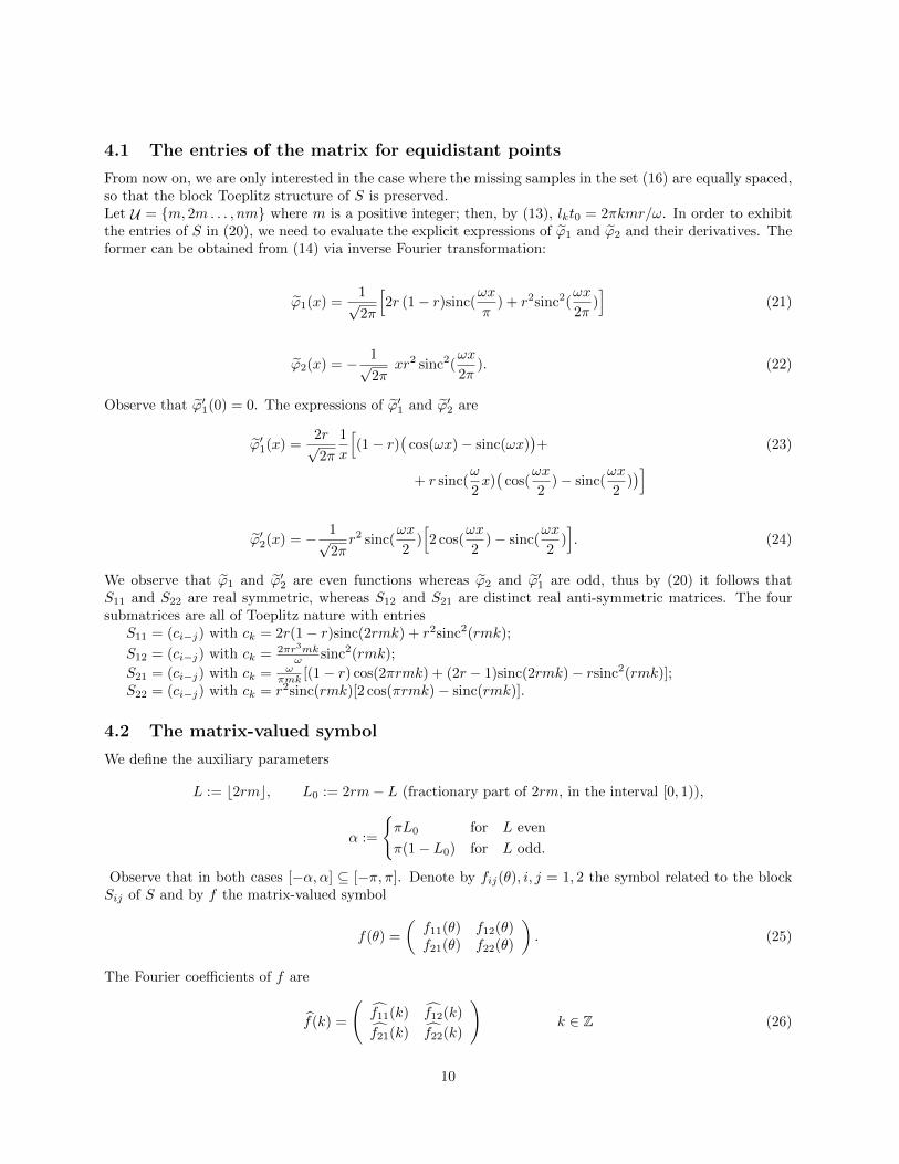
4.1 The entries of the matrix for equidistant points

From now on, we are only interested in the case where the missing samples in the set (16) are equally spaced,so that the block Toeplitz structure of S is preserved.Let U = {m, 2m. . . , nm} where m is a positive integer; then, by (13), lkt0 = 2πkmr/ω. In order to exhibitthe entries of S in (20), we need to evaluate the explicit expressions of ϕ1 and ϕ2 and their derivatives. Theformer can be obtained from (14) via inverse Fourier transformation:

ϕ1(x) =1√2π

[2r (1− r)sinc(

ωx

π) + r2sinc2(

ωx

2π)]

(21)

ϕ2(x) = − 1√2π

xr2 sinc2(ωx

2π). (22)

Observe that ϕ′1(0) = 0. The expressions of ϕ′1 and ϕ′2 are

ϕ′1(x) =2r√2π

1

x

[(1− r)

(cos(ωx)− sinc(ωx)

)+ (23)

+ r sinc(ω

2x)(

cos(ωx

2)− sinc(

ωx

2))]

ϕ′2(x) = − 1√2πr2 sinc(

ωx

2)[2 cos(

ωx

2)− sinc(

ωx

2)]. (24)

We observe that ϕ1 and ϕ′2 are even functions whereas ϕ2 and ϕ′1 are odd, thus by (20) it follows thatS11 and S22 are real symmetric, whereas S12 and S21 are distinct real anti-symmetric matrices. The foursubmatrices are all of Toeplitz nature with entries

S11 = (ci−j) with ck = 2r(1− r)sinc(2rmk) + r2sinc2(rmk);

S12 = (ci−j) with ck = 2πr3mkω sinc2(rmk);

S21 = (ci−j) with ck = ωπmk [(1− r) cos(2πrmk) + (2r − 1)sinc(2rmk)− rsinc2(rmk)];

S22 = (ci−j) with ck = r2sinc(rmk)[2 cos(πrmk)− sinc(rmk)].

4.2 The matrix-valued symbol

We define the auxiliary parameters

L := b2rmc, L0 := 2rm− L (fractionary part of 2rm, in the interval [0, 1)),

α :=

{πL0 for L even

π(1− L0) for L odd.

Observe that in both cases [−α, α] ⊆ [−π, π]. Denote by fij(θ), i, j = 1, 2 the symbol related to the blockSij of S and by f the matrix-valued symbol

f(θ) =

(f11(θ) f12(θ)f21(θ) f22(θ)

). (25)

The Fourier coefficients of f are

f(k) =

(f11(k) f12(k)

f21(k) f22(k)

)k ∈ Z (26)

10

where for each i, j (fij(k)) is the sequence (ck) giving the entries of Sij in Subsection 4.1.

Of course S is not in the form prescribed in (2), but is similar via a permutation matrix to Tn(f) withf as in (25) and according to (2). In formulae we have

ΠSΠT = Tn(f)

with Π of size 2n being the permutation matrix

Π =

eT1 00 eT1...

...eTn 00 eTn

and with ej , j = 1, . . . , n, being the n vectors of the canonical basis of Cn.

In the subsections below we find the explicit expressions of fij which depend on the parity of L and arepiecewise defined on the subintervals (−π,−α), (−α, 0), (0, α) and (α, π). We also observe that fij is evenor odd according with the parity of the sequence of its Fourier coefficients ck, so that f11 and f22 are even,whereas f12 and f21 are odd. Thus it is sufficient to give their expressions only for θ ∈ (0, π).

4.2.1 Even L

f11(θ) =

c11 + 1

m −L

2m2 − θ2πm2 if θ ∈ (0, α)

c11 if θ ∈ (α, π)

f12(θ) =

irmω if θ ∈ (0, α)

0 if θ ∈ (α, π)

where c11 := 2r − r2 − (1− r)L0

m −L2

0

4m2 ,

f21(θ) =

iωθ

4πrm3 (c2 + θ/π) if θ ∈ (0, α)

iωc14πrm3 (θ − π) if θ ∈ (α, π)

f22(θ) =

c22 + L+θ/π

2m2 if θ ∈ (0, α)

c22 if θ ∈ (α, π)

where c1 := L2 − 2mL, c2 := c1 + 2(1− 4r)m+ 2L and c22 := r2 − rL0

m +L2

0

4m2 .

4.2.2 Odd L

f11(θ) =

c11 + 1

2πm2 (−θ + α) if θ ∈ (0, α)

c11 + 1−rm if θ ∈ (α, π)

f12(θ) =

irmω if θ ∈ (0, α)

0 if θ ∈ (α, π)

where c11 := 2r − r2 − (1− r)L0

m −(1−L0)2

4m2 ,

f21(θ) =

iωθ

4πrm3 (c4 + θ/π) if θ ∈ (0, α)

iωc34πrm3 (θ − π) if θ ∈ (α, π)

f22(θ) =

c22 + 1

2πm2 (θ − α) if θ ∈ (0, α)

c22 + rm if θ ∈ (α, π)

where c3 := (1 + L)(1 + L− 2m), c4 := L2 − 2mL− 1 and c22 := r2 − rL0

m + (1−L0)2

4m2 .

11

4.3 A simplified matrix-valued symbol, multigrid methods, and some represen-tations of the true symbol

As well known, several spectral results on block Toeplitz sequences (including those summarized in Section 2)are based on integral formulas in terms of the symbol and specific trigonometric polynomials. The same istrue for the matrix S described in (19) since

v∗Sv =1

2π

∫ π

−πp(θ)∗f(θ)p(θ) dθ, (27)

where v =(xy

)with x = (x1, x2, . . . , xn)T and y = (y1, y2, . . . , yn)T in Cn, whereas p(θ) =

(x(θ)y(θ)

)with x(θ)

and y(θ) trigonometric polynomials isometrically associated to the vectors x and y, respectively, as follows:

x(θ) =

n∑k=1

xkeikθ, y(θ) =

n∑k=1

ykeikθ.

Below we find an interesting analog of the classical Toeplitz representation (27) in terms of a new 2× 2matrix-valued symbol A(t) having a very simplified expression. Let m be the interleaving factor in thepositions U = {m, 2m. . . , nm} of the missing samples.

Theorem 4.1 Let r ∈ (0, 1) and let S be the matrix in (19). Then the following integral formula

v∗Sv =

∫ r

−rP (t)∗A(t)P (t) dt (28)

holds, where

A(t) =

(1− |t| −irsgn(t)/ω

iωt(1− |t|)/r |t|

)t ∈ [−1, 1], (29)

P (t) = (Φ(t),Ψ(t))T and

Φ(t) =

n∑k=1

xke2πimkt , Ψ(t) =

n∑k=1

yke2πimkt. (30)

Proof. From the expressions of the entries of S in (20) with `k = mk, k = 1, . . . n, we have

v∗Sv =√

2π

n∑k,j=1

xkxj ϕ1(m(k − j)t0)+

n∑k,j=1

xjyk ϕ2(m(k − j)t0)+

+

n∑k,j=1

xkyj ϕ1′(m(k − j)t0)+

n∑k,j=1

ykyj ϕ2′(m(k − j)t0)

.By inverse transforming in (14) and changing variables in the integral, we obtain

ϕ1(x) =√

2π

∫ r

−r(1− |t|)eixωt/rdt ϕ2(x) =

√2π i

r

ω

∫ r

−rsign(t)eixωt/rdt .

From this, by using the identity g′(ξ) = iξ g(ξ) we deduce similarly for the derivatives

ϕ1′(x) =

√2πi

ω

r

∫ r

−rt(1− |t|)eixωt/rdt ϕ2

′(x) = −

√2π

∫ r

−r|t|eixωt/rdt .

12

Thus, by reminding that t0 = 2πr/ω by (13), the quadratic form can be written as

v∗Sv =

∫ r

−r(1− |t|)

n∑k,j=1

xk xj e2πim(k−j)tdt− i

r

ω

∫ r

−rsign(t)

n∑k,j=1

xj yk e2πim(k−j)tdt

+ iω

r

∫ r

−rt(1− |t|)

n∑k,j=1

xk yj e2πim(k−j)tdt+

∫ r

−r|t|

n∑k,j=1

yk yj e2πim(k−j)tdt .

Hence, by (30), the expression of the quadratic form becomes

v∗Sv =

∫ r

−r(1− |t|)|Φ(t)|2 dt− i

r

ω

∫ r

−rsign(t)Φ(t)Ψ(t) dt

(31)

+ iω

r

∫ r

−rt(1− |t|)Φ(t)Ψ(t) dt+

∫ r

−r|t||Ψ(t)|2 dt .

Thus formula (28) is proved.

When 1/2 < r < 1 (the main case of interest) the integration domain in (31) can be further restricted.

Corollary 4.1 Let 1/2 < r < 1 and let S,Φ,Ψ, P be as in Theorem 4.1, then

v∗Sv =

∫ 1/2

−1/2

P (s)∗A(s)P (s) ds

where P = (Φ,Ψ)T ; the matrix A(s) is equal to A(s) in (29) if |s| ≤ 1 − r and is the identity matrix if1− r ≤ |s| < 1/2.

Proof. Since 1/2 < r < 1, we may write the first integral in (31) as the sum of the integrals on theintervals [−r,−1/2], [−r, r] and [r, 1/2]. Then we change the variable in the first and the third integral anduse the fact that the function Φ has period 1, obtaining∫ r

−r(1− |t|)|Φ(t)|2 dt =

∫ 1/2

1−rs |Φ(s)|2 ds +

∫ 1/2

−1/2

(1− |s|) |Φ(s)|2 ds −∫ −1+r

−1/2

s |Φ(s)|2 ds.

This can be written as follows∫ r

−r(1− |t|)|Φ(t)|2 dt =

∫ 1/2

−1/2

[s χ[1−r,1/2](s) + (1− |s|)− s χ[−1/2,r−1](s)

]|Φ(s)|2 ds .

By performing similar calculations for the other three integrals in (31), we obtain

v∗Sv =

∫ 1/2

−1/2

[a11(s)|Φ(s)|2 + a12(s)Φ(s)Ψ(s) + a21(s)Φ(s)Ψ(s) + a22(s)|Φ(s)|2

]ds

where

a11(s) =

{(1− |s|) if |s| ≤ 1− r1 if 1− r ≤ |s| < 1/2

a22(s) =

{|s| if |s| ≤ 1− r1 if 1− r ≤ |s| < 1/2

a12(s) =

{−i rω sign(s) if |s| ≤ 1− r0 if 1− r ≤ |s| < 1/2

a21(s) =

{iωr s(1− |s|) if |s| ≤ 1− r0 if 1− r ≤ |s| < 1/2.

13

This concludes the proof.

The results of Theorem 4.1 and Corollary 4.1 easily extend to the case where the missing samples arenot equally spaced. Indeed it suffices to replace the functions Φ and Ψ in (30) by

Φ(t) =

n∑k=1

xke2πi`kt , Ψ(t) =

n∑k=1

yke2πi`kt. (32)

Now we can discuss the spectral properties of the simplified symbol A(t) in (29). The first key observationis that, since A12(t)A21(t) = |t|(1− |t|), A(t) has rank equal to 1 independently of t so that the spectrum isgiven by 0 and 1 (that is the trace of A(t)).

Second we observe that A(t) is similar to the symmetric matrix-valued symbol

Asym(t) =

(1− |t|

√|t|(1− |t|)√

|t|(1− |t|) |t|

).

Indeed if we prove that A(t) is similar via a constant similarity transformation to a Hermitian symbol,then by Remark 2.1 we would have that all the eigenvalues of S are real, belonging to the interval [0, 1].Unfortunately the similarity transformation matrix is not constant with respect to t so that we cannot applythe intersection statement in Remark 2.1. This negative fact is structural in the sense that for every constantinvertible matrix Q, a trivial computation shows that QA(t)Q−1 is not always Hermitian: however this factdoes not imply that the same is true for f(θ).Moreover, we observe that, by a change of variable, the integral formula (28) may be written as

v∗Sv =1

π

∫ πr

−πrP (θ)∗A(θ/π)P (θ) dθ, (33)

where

Φ(θ) :=

n∑k=1

xkei2mkθ, Ψ(θ) :=

n∑k=1

ykei2mkθ (34)

for θ ∈ [−π, π] and P (θ) = (Φ(θ),Ψ(θ))T .

It is intriguing to compare (33) with the classical representation formula (27) relating a block Toeplitzmatrix and its symbol, which we remind below:

v∗Sv =1

2π

∫ π

−πp(θ)∗f(θ)p(θ) dθ

(with p(θ) different from P (θ)). We can guess that the product

F (θ) = 2A(θ/π) · χ[−πr,πr](θ) (35)

plays the role of a symbol (a simplified symbol), but with a much simpler expression when compared withthe true symbol f(θ).

Therefore we try to determine the relations between the spectral properties of the block Toeplitz sequenceunder study and the analytical/spectral features of the simplified symbol.

First we put in relation the simplified symbol and the true symbol: to this end classical tools used whendesigning multigrid methods are really useful (see [7]: equation (4.7) in Proposition 4.1 where g := 2m, pidentically 1 and Section 6.1 therein for a discussion on the Toeplitz case). In fact the integral formula (33),in matrix terms, can be read as

ΠSΠT = Tn(f) = UTT2nm(F )U

14

where U = U ⊗ I2 is the “cutting” matrix of size 4nm × 2n, with Uij = 1 if and only if j = (i − 1)2m + 1and zero otherwise. Therefore we have

f(θ) =1

2m

2m−1∑j=0

F

(θ + 2πj

2m

)=

1

m

2m−1∑j=0

A

(θ + 2πj

2mπ

)· χ[−πr,πr]

(θ + 2πj

2m

). (36)

We observe that the characteristic function present in the expression (35) for F , evaluated in the varioussub-intervals given by the change of variable θ 7→ θ+2πj

2m , becomes identically 1 or identically 0 most of thetimes so that, taking into account the definition domain of A(t), the symbol f(θ) in (36) becomes

f(θ) =1

m

bL/2c∑

j=−bL/2c

A

(θ + 2πj

2mπ

)

−A(θ − Lπ2mπ

)· χ[−π,−πL0](θ) (37)

−A(θ + Lπ

2mπ

)· χ[πL0,π](θ)

}if L is even or

f(θ) =1

m

bL/2c∑

j=−bL/2c

A

(θ + 2πj

2mπ

)

+A

(θ + (L+ 1)π

2mπ

)· χ[−π,−π(1−L0)](θ) (38)

+A

(θ − (L+ 1)π

2mπ

)· χ[π(1−L0),π](θ)

}if L is odd.

Formulae (37) and (38) can be considered as an alternative representation of f in place of that given inSubsection 4.2.

5 Numerical results (vs Theoretical results)

First of all we concentrate our attention on the distribution results (and a fortiori on the cluster sets). Tothis end the first task is to check the assumptions of Theorem 2.3: the latter means that the range R(f) (theunion of the ranges of λ1(f(θ)) and λ2(f(θ))) must not disconnect the complex plane. The main difficultyrelies on the several parameters involved in the analytical expression of the symbol f(θ). Nevertheless thenext proposition answers in the positive to our question, as it will be explicitly emphasized in Theorem 5.1.

Proposition 5.1 Let αi, i = 1, . . . , l be real numbers belonging to [0, 1] with l ≤ 2l′, both l, l′ being positive

integer numbers. Let si, i = 1, . . . , l be a collection of signs i.e. si ∈ {±1}, i = 1, . . . , l, let ν =∑li=1 si, and

finally let γ be a nonzero complex value. For every i = 1, . . . , l define

Ai =

(1− αi γ−1si

γsi(1− αi)αi αi

)and

A =1

l′

l∑i=1

Ai. (39)

15

If ν ≥ 0 then the eigenvalues of A, namely λ1(A) and λ2(A), are both real nonnegative with

0 ≤ λ1(A) ≤ l

2l′≤ λ2(A) ≤ l

l′≤ 2. (40)

Moreover for ν = 0 we have

λ1(A) =l −∑li=1 αil′

,

λ2(A) =

∑li=1 αil′

.

If ν < 0 then the eigenvalues of A can take either the same form as in (40) or the form

λ1,2(A) =l

2l′± iβ,

l

2l′≥ β > 0. (41)

Proof. It is enough to observe that every Ai can be seen as a sampling of the simplified symbol A(t) ona given point ti: therefore each Ai is a rank-one matrix with trace 1. Hence, by (39), the trace of A is givenby

tr(A) =l

l′,

while a simple check (again by (39)) shows that

det(l′A) = (l −l∑i=1

αi)

l∑i=1

αi − νl∑i=1

(1− αi)αi

with

λ1,2(A) =1

2

[tr(A)±

√tr2(A)− 4det(A)

]. (42)

Now assume ν ≥ 0. Since∑li=1 αi ∈ [0, l], it follows that (l −

∑li=1 αi)

∑li=1 αi ∈ [0, l2/4] with minimum

attained when∑li=1 αi = 0 or

∑li=1 αi = l and maximum attained for

∑li=1 αi = l/2. Since

l∑i=1

(1− αi)αi ≥ 0

it directly follows that det(l′A) ≤ l2/4. In order to find a lower bound, we perform a direct computation sothat, taking into account that ν ≤ l we have

det(l′A) = (l −l∑i=1

αi)

l∑i=1

αi − νl∑i=1

(1− αi)αi

≥ (l −l∑i=1

αi)

l∑i=1

αi − ll∑i=1

(1− αi)αi

= l

l∑i=1

(αi)2 −

(l∑i=1

αi

)2

= ‖e‖22‖a‖22 − (eTa)2 ≥ 0,

where e is the vector of length l of all ones, a is the vector whose i-th component is αi, and where in thelast line we have used the Cauchy-Schwartz inequality. Therefore

√tr2(l′A)− 4det(l′A) ∈ [0, l] and the

estimates in (40) directly follow.

16

With analogous computation the case of ν ∈ [−l, 0] leads to the estimate det(l′A) ∈ [0, l2/2] so thateither (40) is true or (41) is true and the proof is complete.

In the sequel, we use the notation Sn to emphasize that the matrix S has inner blocks of size n whichcan arbitrarily grow.

Theorem 5.1 The eigenvalues of the sequence {Sn} are distributed as λ1(f(θ)) and λ2(f(θ)) that is

{Sn} ∼λ (f, I1)

according to the notations in Theorem 2.3.

Proof. As already proved Sn is similar to Tn(f) and, according to (36), the symbol f(θ) is such that,for any fixed θ, the matrix f(θ) is of the form (39) with l′ = m, l ≤ 2m and γ = iω/r. Therefore, byProposition 5.1 the set R(f) is a subset of the cross K in the complex plane given by

K = {z ∈ C : Im(z) = 0,Re(z) ∈ [0, 2]}⋃{

z ∈ C : Re(z) =l

2m, Im(z) ∈ [−1, 1]

}.

Since K does not disconnect C, the same does R(f) and the desired result follows from Theorem 2.3.

Therefore, according to the discussion in Subsection 2.2, n eigenvalues of S = Sn behave as the function

θ 7→ λ1(f(θ))

and the remaining n eigenvalues of S = Sn behave as the function

θ 7→ λ2(f(θ))

or equivalently (−π +

2πj

n, λ

(k)j

)≈(−π +

2πj

n, λk

(f

(−π +

2πj

n

)))are approximate sampling values of the function λk(f(θ)), k = 1, 2.

At this point it is clear that our goal has to be the understanding as much as possible of the expressionof λk(f(θ)), k = 1, 2.

The information is in fact contained in the representations (37) and (38), and in those of Subsection 4.2.In connection with Proposition 5.1, a careful analysis shows that

l ∈ {L,L+ 1}, ν ∈ {0,±1}.

In fact, in formula (36), the sub-domains

Ij =

[2j − 1

2m,

2j + 1

2m

]obtained from the affine transform θ 7→ θ+2πj

2m , θ ∈ [−π, π], are such that χ[−πr,πr](θ)∣∣Ij is either identically

zero or identically one most of the times.As a consequence, when ν = 0, the symbol is lower triangular so that the eigenvalues of f(θ) are the

diagonal entries. i.e.

λ1(f(θ)) = r2 − rL0

m+

L20

4m2,

λ2(f(θ)) = 2r − r2 − (1− r)L0

m− L2

0

4m2,

17

for L even and θ ∈ [−π, π]\[−α, α] or

λ1(f(θ)) = r2 + (1− L0)r

m+

(1− L0)2

4m2,

λ2(f(θ)) = 2r − r2 − (1− L0)(1− r)m

− (1− L0)2

4m2,

for L odd and θ ∈ [−π, π]\[−α, α].In the remaining domain, both for even and odd L, an explicit computation shows that

|λ1(f(θ))− r2| ≤ r

m+O

(1

m3

), (43)

|λ2(f(θ))− (2r − r2)| ≤ 1− rm

+O

(1

m3

)(44)

so that R(f) is made by 4 points V1, V2, V3, V4, where for m tending to infinity we have V1 = V2 = r2 andV3 = V4 = 2r−r2, i.e. two parabola symmetrically placed with respect to the first bisectrix with r2 ≤ 2r−r2

for r ∈ [0, 1] and equality only at r = 0, r = 1 (we recall in any case that the parameter r lies in the physicaldomain (0, 1)).

Concerning the localization results we do not try to apply Theorem 2.2, because of its intrinsic difficulty.Instead we follow the discussion in Remark 2.1: indeed, we have been not able to prove the existence of aconstant similarity transform which makes the symbol Hermitian and this leaves the door open for furtherinvestigations, in the sense of items s1 and s2 and of the related discussion in the Introduction.

One of the desired properties (required by the algorithms used for treating the considered signal-restoration problem with missing data) is the fact that all the eigenvalues of S = Sn are nonnegativeand strictly less than one.

Indeed the asymptotic values r2 and 2r − r2 have the desired property and the same occurs for everyn for the eigenvalues of S = Sn, when m is large. The problem is nontrivial when m is moderate, but afiner analysis, taking into account that L0 depends on r, shows that the two eigenvalues of the symbol havealways essential infimum and essential supremum in the interval (0, 1).

5.1 Numerical evidences

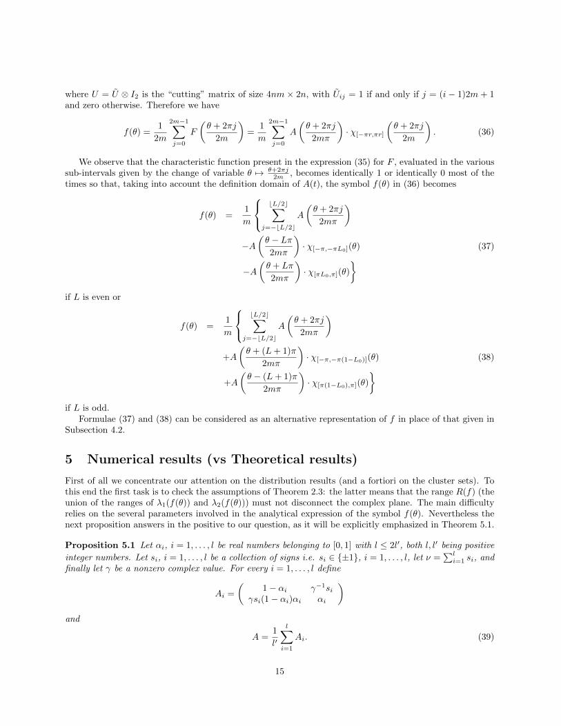
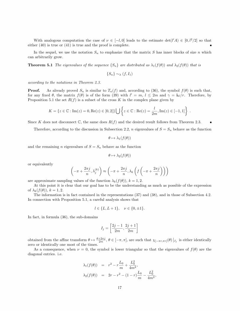
The following set of numerical tests confirms that the spectrum of S = Sn is well described by the range ofthe two functions λ1(f(θ)) and λ2(f(θ)) according to Theorem 5.1. To this end the eigenvalues of the 2× 2matrix valued symbol f(θ) are sampled over 1000 equi-spaced points on the natural domain I1 = [−π, π].The tests are performed using MatLab in double precision.

Figures 1–3 show the eigenvalues of S = Sn and the values of λ1(f(θ)) and λ2(f(θ)), for several combi-nations of the parameters. The imaginary part of the computed eigenvalues has a size comparable to themachine precision and therefore we can safely claim that the eigenvalues of Sn are purely real. Furthermore,the agreement among the eigenvalues and R(f) is impressive, giving evidence of the result described inTheorem 5.1 (see the discussion after the theorem for a ‘visual’ interpretation of the result that is perfectlyvisible in our tests).

Now we focus our attention on the behavior of the extremal eigenvalues. Indeed it is proved that

limm,n→∞

λk(Sn) = r2, limm,n→∞

λ2n−k(Sn) = 2r − r2 (45)

for every fixed k independent of n (see also [1]), where we have assumed the ordering λ1(Sn) ≤ λ2(Sn) ≤· · · ≤ λ2n(Sn).

Figure 4 shows that a similar behavior can be observed for the range of the two eigenvalues of f , forlarge m (they approach the limits in (45), symmetric around the line y = r, r ∈ [0, 1]). More specificallyin Figure 4 (c) we see that for r = 0.8, n = 50 and large m the maximal eigenvalue of S = Sn differs from

18

0.4 0.5 0.6 0.7 0.8 0.9 1−5

0

5x 10

−15

0.4 0.5 0.6 0.7 0.8 0.9 1−8

−6

−4

−2

0

2

4

6

8x 10

−15

0.4 0.5 0.6 0.7 0.8 0.9 1−2

−1.5

−1

−0.5

0

0.5

1

1.5

2x 10

−15

m = 5 m = 12 m = 21

Figure 1: The ◦ depict the eigenvalues of S for n = 100 and the × depict the range of the eigenvalues of ffor r = 0.7.

0.2 0.4 0.6 0.8 1−3

−2

−1

0

1

2

3x 10

−16

0.5 0.6 0.7 0.8 0.9 1−4

−3

−2

−1

0

1

2

3

4x 10

−16

0.7 0.8 0.9 1 1.1−1.5

−1

−0.5

0

0.5

1

1.5

2x 10

−15

r = 0.6 r = 0.75 r = 0.9

Figure 2: The ◦ depict the eigenvalues of S for n = 100 and the × depict the range of the eigenvalues of ffor m = 8

0.4 0.5 0.6 0.7 0.8 0.9 1−1

−0.5

0

0.5

1

0.4 0.5 0.6 0.7 0.8 0.9 1−3

−2

−1

0

1

2

3x 10

−16

0.4 0.5 0.6 0.7 0.8 0.9 1−3

−2

−1

0

1

2

3

4x 10

−15

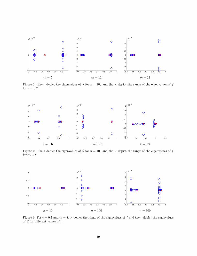
n = 10 n = 100 n = 300

Figure 3: For r = 0.7 and m = 8, × depict the range of the eigenvalues of f and the ◦ depict the eigenvaluesof S for different values of n.

19

0 20 40 60 80 100−0.2

0

0.2

0.4

0.6

0.8

1

1.2

0 20 40 60 80 100−0.2

0

0.2

0.4

0.6

0.8

1

1.2

0 20 40 60 80 10010

−16

10−15

10−14

10−13

10−12

(a) (b) (c)

Figure 4: For r = 0.8 and n = 50 versus m = 1, . . . , 100: (a) ◦ are λmax(S) and × are λmin(S), (b) ◦are λmax(f) and × are λmin(f) (introduced in Definition 2.1), (c) the dashed curve depicts |λmax(S) −λmax(f)|/|λmax(S)| while the solid curve depicts |λmin(S)− λmin(f)|/|λmin(S)|.

0 10 20 30 400.4

0.5

0.6

0.7

0.8

0.9

1

1.1

0 50 100 150 2000.4

0.5

0.6

0.7

0.8

0.9

1

1.1

0 100 200 300 400 500 6000.4

0.5

0.6

0.7

0.8

0.9

1

1.1

(a) (b) (c)

Figure 5: For r = 0.8 and m = 3 varying n, ◦ are the eigenvalues of S while × denote R(f): (a) n = 20, (b)n = 100, (c) n = 300.

λmax(f) for less than 10−14, while λmin(f) and the minimal eigenvalue of S = Sn are equal up to the machineprecision (for m = 1 the error is only relatively big since all the involved quantities are of the order of themachine precision, see Figures 4 (a)–(b)).

Figure 5 shows that the eigenvalues of S are all contained in R(f) with the only exception of (O(log(n)))that are far away from the 4 points forming R(f), but still in the envelope of the range (λmin(f), λmax(f));see [11] and [4, p. 143] for the study of a similar situation in the case of a scalar-valued symbol.

Figure 6 shows an interesting asymptotic behavior of R(f) as the parameter m tends to infinity: in thelimit two of the points forming R(f) collapse from above to r2 and the other two collapse from below to2r − r2 according to (43) and (44), respectively.

The last test shows how fast the minimum eigenvalue of S approaches λmin(f). Figure 7 shows thatincreasing n, λmin(S) converges exponentially to λmin(f): see conjectures s1 and s2.

We finally remark that the exponential convergence (with difference going to zero monotonically as e−n)is the fastest rate we can have for block Toeplitz matrices, according to the result conjectured in [13] andformally proved by Tilli in [19].

6 Conclusions and open problems

We have considered a special type of signal restoration problem where some of the sampling data are notavailable. The formulation leads to a large nonsymmetric block Toeplitz matrix which can be associated

20

0 200 400 600 800 10000.5

0.6

0.7

0.8

0.9

1

1.1

0 200 400 600 800 10000.5

0.6

0.7

0.8

0.9

1

1.1

0 200 400 600 800 10000.5

0.6

0.7

0.8

0.9

1

1.1

(a) (b) (c)

Figure 6: R(f) for r = 0.8 varying m: (a) m = 4, (b) m = 31, (c) m = 101.

0 10 20 30 40 5010

−25

10−20

10−15

10−10

10−5

100

0 10 20 30 40 5010

−25

10−20

10−15

10−10

10−5

100

0 10 20 30 40 5010

−25

10−20

10−15

10−10

10−5

100

r = 0.7, m = 9 r = 0.9, m = 4 r = 0.8, m = 11

Figure 7: The dashed curve depicts the reference function e−n, while the solid curve depicts |λmin(S) −λmin(f)|/|λmin(f)|, versus n = 1, . . . , 50.

21

to a 2 × 2 matrix-valued symbol f(θ) that has been identified and studied. The use of recent results onthe eigenvalue localization and distribution of block Toeplitz matrix-sequences, has been of great help indescribing the cluster sets, the spectral distribution, and the localization areas/extremal behavior of thespectrum of the double window matrix, although the information is not yet complete.

In any case, we believe that further developments in the asymptotic theory for nonsymmetric symbolswill be possible, providing a very effective tool to predict the full dependence of the spectral behaviour onthe parameters. In addition, the applicative impact of such future results could address the most appropriatechoice of free parameters in the design of transmission devices.

Furthermore, the theory is very general and so we are confident that our analysis can be extended alongthe following lines:

• The case of arbitrary positions of missing samples (one difficulty is given by the lack of spectral resultsrelating a non-symmetric matrix to its submatrices). The more specific case where the positions of themissing samples are approximately described by a nonlinear function will lead to Generalized LocallyToeplitz structures whose spectral theory is well developed (see [17, 14]).

• The case of s > 2 channels (leading to s× s matrix-valued symbols).

• The case of 2D or 3D images in place of a one-dimensional signal F (leading to 2- or 3-level Toeplitzstructures with symbol depending on 2 or 3 variables). This new reconstruction problem presents someanalogies with the inpainting problem, investigated with the help of structured matrices by R. Chanand collaborators in a series of papers (see e.g. [5]).

References

[1] P. Brianzi, V. Del Prete, Stability of the Recovery of Missing Samples in Derivative Oversampling,Sampl. Theory in Signal and Image Process. 10 (2011) 191–210.

[2] A. Bottcher, S. Grudsky, On the condition numbers of large semi-definite Toeplitz matrices, LinearAlgebra Appl. 279 (1998) 285–301.

[3] A. Bottcher, S. Grudsky, E. Ramirez de Arellano, On the asymptotic behavior of the eigenvectors oflarge banded Toeplitz Matrices, Math. Nachr. 279 (2006) 121–129.

[4] A. Bottcher, B. Silbermann, Introduction to Large Truncated Toeplitz Matrices, Springer, New York,1999.

[5] J.F. Cai, R.H. Chan, Z.W. Shen, A Framelet-Based Image Inpainting Algorithm, Appl. Comput. Har-mon. Anal. 24 (2008) 131–149.

[6] M. Donatelli, M. Neytcheva, S. Serra-Capizzano, Canonical eigenvalue distribution of multilevel blockToeplitz sequences with non-Hermitian symbols, Operator Theory: Adv. and Appl. 221 (2012) 273–295.

[7] M. Donatelli, S. Serra-Capizzano, D. Sesana, Multigrid methods for Toeplitz linear systems with differentsize reduction, BIT 52 (2012) 305–327.

[8] P.J.S.G. Ferreira, The stability of a procedure for the recovery of lost samples in band-limited signals,Signal Processing 40 (1994) 195–205.

[9] W. Rudin, Real and Complex Analysis, McGraw-Hill, New York, 1974.

[10] D.M.S. Santos, P.J.S.G. Ferreira, Reconstruction from Missing Function and Derivative Samples andOversampled Filter Banks, Proceedings of the IEEE International Conference on Acoustics, Speech, andSignal Processing, ICASSP 3 (2004) 941–944.

22

[11] S. Serra-Capizzano, Preconditioning strategies for Hermitian Toeplitz systems with nondefinite gener-ating functions, SIAM J. Matrix Anal. Appl. 17 (1996) 1007–1019.

[12] S. Serra-Capizzano, On the extreme eigenvalues of Hermitian (block) Toeplitz matrices, Linear AlgebraAppl. 270 (1998) 109–129.

[13] S. Serra-Capizzano, How bad can positive definite Toeplitz matrices be?, Numer. Funct. Anal. Optim.,21 (2000) 255–261.

[14] S. Serra-Capizzano, Generalized Locally Toeplitz sequences: spectral analysis and applications to dis-cretized Partial Differential Equations, Linear Algebra Appl. 366 (2003) 371–402.

[15] S. Serra-Capizzano, P. Tilli, Extreme singular values and eigenvalues of non Hermitian block Toeplitzmatrices, J. Comput. Appl. Math. 108 (1999) 113–130.

[16] S. Serra-Capizzano, Spectral and computational analysis of block Toeplitz matrices having nonnegativedefinite matrix-valued generating functions, BIT 39 (1999) 152–175.

[17] P. Tilli, Locally Toeplitz sequences: spectral properties and applications, Linear Algebra Appl. 278(1998) 91–120.

[18] P. Tilli, A note on the spectral distribution of Toeplitz matrices, Linear Multilin. Algebra 45 (1998)147–159.

[19] P. Tilli, Universal bounds on the convergence rate of extreme Toeplitz eigenvalues, Linear Algebra Appl.366 (2003) 403–416.

[20] J.M. Varah, The prolate matrix, Linear Algebra Appl. 187 (1993) 269–278.

[21] N.L. Zamarashkin, E.E. Tyrtyshnikov, On the distribution of eigenvectors of Toeplitz matrices withweakened requirements on the generating function, Russ. Math. Surv. 522 (1997) 1333–1334.

23