~ 1 ~

Symbiosis and Coordination of Macroeconomic Policies in a

Monetary Union

Georgios Chortareas

School of Management & Business, King’s College London,

and Department of Economics, National & Kapodistrian University of Athens

georgios.chortareas@kcl.ac.uk

and

Christos Mavrodimitrakis1

School of Economics and Finance, Queen Mary University of London, and

Department of Economics, National & Kapodistrian University of Athens

xmaurod@econ.uoa.gr

Abstract

This paper deals with strategic policy interactions in a monetary union. We use a static two-country

monetary-union model, which incorporates the key features of the New-Keynesian framework. We

investigate the policy mix outcome under non-conflicting but different objectives when the two policy

instruments can directly affect inflation. Thus, we provide a reconciliation of the early literature, which is

mostly based on the supply-side of the economy with the most recent literature, which mainly focuses on

the demand side. We consider the short-run macroeconomic stabilization and welfare implications of the

fiscal-monetary policy interactions at both the union and national levels. We compare and contrast the

alternative strategic regimes (simultaneous-move, fiscal/monetary leadership) in the monetary union and

we analyze both the horizontal (across governments) and the vertical (between the monetary and the fiscal

authorities) coordination problems. We define the impact that the policies’ direct effects on inflation has

on (i) fiscal authorities’ cooperation, (ii) policies’ cyclicality, and (iii) the alternative strategic regimes

(symbiosis). We draw important results on the preferable strategic and fiscal regimes for the monetary

authority.

1 (Corresponding Author) Queen Mary University of London, School of Economics & Finance, Graduate Centre,

Bancroft Road, London E1 4DQ, UK. Email: c.mavrodimitrakis@qmul.ac.uk. Tel: +44 (0)7546090138.

~ 2 ~

Keywords: Monetary union; Fiscal/monetary policies; Coordination; Symbiosis; Strategic regimes.

JEL Classification: E52; E61; E62; E63; F45.

1. Introduction

There has been more than fifteen years since the official launch of the Economic and Monetary Union

(EMU) in Europe, the “greatest monetary reform since Bretton Woods” (Buti, 2003, p. 24). However, the

consequences of fiscal and monetary policy interactions still remain an issue among both academia and

policymakers. The recent travails of the Eurozone reveal that the institutional structure of policymaking has

been imperfect and motivate further research on fiscal-monetary policy interactions in monetary unions.

Monetary policy is conducted by an independent supranational authority, the European Central Bank

(ECB), while fiscal policy remains decentralized at national level, respecting the debt sustainability

constraint imposed by the European Union (EU), meaning the Stability and Growth Pact (SGP), and more

recent fiscal developments described by the Fiscal Compact2 (FC). In this framework, fiscal policy remains

the macroeconomic tool of national authorities to stabilize their economies under country-specific shocks.

However, non-coordinated fiscal policies in national level may create externalities to other member-states,

creating inefficiencies. This might induce the possibility of policy coordination.

Beetsma and Giuliodori (2010) provide an overview of the research on the macroeconomic costs and

benefits of the EMU. In Sections 6 and 7, the authors examine fiscal policy and conflicts of interest in the

monetary union, as well as fiscal spillovers and coordination. Formal analysis of the policy mix and fiscal

policies’ coordination requires a framework to model strategic interactions among fiscal authorities and the

common central bank.3 In particular, assumptions regarding authorities’ objectives, their ability to commit

and the timing of their decisions are at the center of the analysis. In a recent paper, Foresti (2017) analyzes

the literature on strategic fiscal/monetary policy interactions in a monetary union. The author presents a

generic theoretical framework in order to highlight the main points of the literature, regarding uncertainty

issues, authorities’ preferences, the role of commitment to policy rules, and coordination. All these issues

have regained interest due to the Eurozone sovereign debt crisis, being part of the appropriate institutional

framework of policymaking in the EMU.

Following Plasmans et. al. (2006), the literature has been mainly focused on two policy interactions:

(i) the links between deficits, debts, inflation and interest rates via the (dynamic) government budget

constraints, and (ii) the links between fiscal and monetary policies in a macroeconomic stabilization

2 Its official name is “The Treaty on Stability, Coordination and Governance” (TSCG). 3 To quote Fragetta and Kirsanova (2010, p. 856), “…there is little doubt that authorities can act strategically”.

~ 3 ~

perspective. This paper follows the second strand of the literature, abstracting from important long-run

issues that are related to fiscal policy, such as debt sustainability.4 To quote Uhlig (2003, p. 43), we are

dealing with the ‘…day-to-day policy task of responding to business cycle shocks’. The literature so far has

offered a plethora of different modeling assumptions that provided mixed results, while general conditions

for cooperation and commitment irrelevance provided by Kempf and von Thadden (2013) follow the lines

of the traditional Barro-Gordon (1983) set-up, where the effects of monetary and fiscal policies are often

set to work only on the supply side of the economy. According to Plasmans et. al. (2006), such an approach

seems rather narrow, considering also that the supply-side effects of monetary and fiscal policies may in

practice be of limited relevance, as they often take a very long time to materialize. On the contrary, the

most recent literature is based on the New-Keynesian framework, which focuses on the demand side of the

economy, where supply is often held fixed.

This paper proposes a unified theoretical framework to analyze strategic policy interactions in a

monetary union. We use a static representation of the New-Keynesian model, following mainly Andersen

(2005, 2008). We assume that the two (for simplicity) member-states in the monetary union are

interconnected via a trade effect and a terms-of-trade effect, and that the policy instruments, namely the

country-specific fiscal stances and the common nominal interest rate, can also directly affect country-

specific inflation. Fiscal policy can have either positive or negative direct effects on inflation, as various

fiscal instruments can have (positive/negative) short-run effects on the supply-side of the economy (see,

e.g., Andersen, 2005, 2008; Debrun, 2000), whereas monetary policy can have a direct positive effect on

inflation, following mainly the cost channel (Ravenna and Walsh, 2006). Our motivation is to provide a

reconciliation between the early literature that was mainly based on the supply-side of the economy with

the most recent one that is mainly focused on the demand side. In the latter case, the Phillips curve is only

affected by the output gap, which means that the two policy instruments are perfect substitutes in the

stabilization process. By comparing the two cases, we mainly focus on the ordering of moves and the

resulting cyclical behavior on the part of the authorities, for both cases of decentralized and centralized

fiscal policies, where the latter case defines fiscal authorities’ cooperation. We thus investigate the policy

mix and the coordination problem in a monetary union under non-conflicting but different objectives, when

both policy instruments can directly affect inflation. Beetsma and Debrun (2004) distinguish the

coordination problem between a horizontal (across governments) coordination problem and a vertical

(between the monetary and the fiscal authorities) one. By non-conflicting objectives we mean that all the

authorities agree on the ideal targets of the concerned macroeconomic variables, being their long-run

4 For example, Aguiar et. al. (2015) study fiscal and monetary policies in a monetary union with the potential for rollover crises in

sovereign debt markets.

~ 4 ~

equilibrium values (Uhlig, 2003). However, objectives may differ, as the national fiscal authorities care

about fiscal stance stabilization and not about inflation. This creates the policy conflict (Kempf and von

Thadden, 2013).

In a series of critical papers, Dixit and Lambertini (2001, 2003a) studied strategic policy interactions

(pure macroeconomic stabilization) in a monetary union in a Barro-Gordon (1983) framework where fiscal

policy can also affect (common) inflation, together with monetary policy, while the monetary authority is

concerned with country-specific data. The main results are: (i) under conflicting objectives, the

simultaneous-move strategic regime is inferior to any leadership regime, while (ii) under non-conflicting

objectives, there is symbiosis of monetary and fiscal policies, in that the actual targets can be obtained

irrespective of the ordering of moves, of fiscal authorities’ cooperation or of identical preference priorities.

Under conflicting objectives, the Nash game produces a sub-optimal race with fiscal expansion aimed at

raising output and monetary contraction aimed at offsetting the effect of fiscal expansion on inflation, which

yields extreme outcomes. The leadership regime, instead, produces improved outcomes, as the leader

moderates its policy in anticipation of the follower’s reaction, who moderates its policy, too.5 Beetsma and

Bovenberg (1998), following Alesina and Tabellini (1987), assume that the monetary authority directly

controls the common inflation rate, while they also incorporate a government budget constraint. The authors

find that fiscal policies’ coordination is welfare-reducing, as it makes the fiscal authorities to set a high tax

rate in order to induce a relax of their budget constraints through an expansionary monetary policy, hence

strengthening their strategic position relative to the monetary authority. In this model, monetary unification

is welfare-enhancing.

Kempf and von Thadden (2013) provide the general conditions for the irrelevance of the ECB’s

commitment capacity and the sequencing of moves (symbiosis result), as well as for fiscal policies’

coordination irrelevance, in monetary unions under both private and fiscal spillovers, combining the work

of Dixit and Lambertini (2001, 2003a) and Chari and Kehoe (2008) in a unified framework. The private

spillovers refer to the (wage) decisions by (multiple) private agents (non-coordinated wage setters) within

countries (Chari and Kehoe, 2008).6 The monetary authority is concerned with country-specific data, there

is a common inflation rate, and the comparison between the two fiscal regimes is made on union-wide

equilibrium solutions. The authors consider alternative commitment patterns (leadership regimes) in that

each player (the private sector; fiscal authorities; the monetary authority) moves at a particular stage of the

game, where all private agents act at the same stage. The fiscal authorities act at the same stage, too. The

5 In a closed-economy setting, the superiority of the fiscal leadership regime is also stressed by Dixit and Lambertini (2003b) and

Hughes Hallett and Weymark (2007), as it provides a regime of implicit coordination between the authorities. 6 In the Barro-Gordon (1983) framework, instead, there exists a representative private sector.

~ 5 ~

sufficient conditions are that the direct spill-over effects must have no strategic significance and that the

number of instruments must match the number of squared gaps in all authorities’ payoff functions. If further

all the authorities agree on the objectives, then the bliss points can be also achieved. In the absence of those

conditions, both cooperation and commitment (the sequence of moves) matter, while the difference between

the non-cooperative and the cooperative outcome depends on the number of countries in the monetary

union. The authors clearly show that the monetary union benefits from fiscal authorities’ cooperation under

fiscal leadership.

The above discussion on the symbiosis result shows that it only holds under specific assumptions of

the model. In the opposite case, both coordination and timing issues become relevant, creating a policy-mix

bias (Foresti, 2017). Since the official launch of the EMU, there are a lot of papers that deal with the

macroeconomic policy mix, fiscal authorities’ cooperation, and the sequencing of moves in monetary

unions. Banerjee (2001) allows for fiscal policies to be subject to potential time inconsistencies, while

comparing different scenarios of commitment and discretion. The author finds that moving from the

scenario of full discretion to other scenarios results in lower inflation and higher expenditure at the expense

of lower output for the full commitment and the fiscal commitment ones, whereas for the monetary

commitment we end up with lower public spending. Godbillon and Sidiropoulos (2001) show that

delegation of fiscal policy to a council of country representatives and monetary policy to a council of

governors is the appropriate institutional design to reduce the inflation bias and better stabilize regional

idiosyncratic supply and demand shocks in a monetary union. Lambertini and Rovelli (2004) show that a

‘vertical’ coordination problem arises even in an extremely simple setting of a simultaneous-move game in

a static two-country monetary-union model, where the two countries are identical and there are no

interconnections between them. The authors further show that the common central bank prefers national

fiscal authorities’ cooperation in minimizing a union-wide welfare function that also includes price stability.

Cavallari and Di Gioacchino (2005) show that fiscal authorities’ cooperation leads to favorable outcomes

for output under demand/supply shocks and for inflation under demand shocks, while overall policy

coordination improves macroeconomic stabilization only under demand shocks. The authors further show

that monetary-fiscal symbiosis vanishes when there are other policy goals than cyclical stabilization, in

particular costly policy instruments, as there must also be agreement on preferences’ weights. Della Posta

and De Bonis (2009) reject the symbiosis result in the presence of asymmetric shocks, showing that policy

coordination can be welfare improving even if the authorities have equal targets. Di Bartolomeo and Giuli

(2011) also reject the symbiosis result in a closed-economy setting, when there is uncertainty about the

effectiveness of the policy instruments.

~ 6 ~

Oros and Zimmer (2015) consider the impact of political (central bank) transparency on the policy

mix in a monetary union under monetary policy transmission heterogeneity. The authors conclude that

when the monetary transmission mechanism is relatively weak, higher monetary uncertainty may contribute

to reduce inflation expectations, improving macroeconomic performance. Von Hagen and Mundschenk

(2003) show that under strict inflation targeting the central bank controls union-wide output gap, while the

national fiscal authorities determine the distribution of aggregate demand between them, engaging in a

purely distributional game with inefficient outcomes unless policies are coordinated. Uhlig (2003) shows

that in the absence of fiscal shocks and symmetrical countries size-wise, all fiscal authorities would be

better off under a cooperative equilibrium characterized by a common fiscal policy of zero deficits. Ferre

(2005) finds that in expansive phases of the economy, fiscal authorities’ cooperation leads to a higher

deficit, while in Ferre (2008) the author shows that the non-cooperative case leads to a more volatile union-

wide fiscal stance. Beetsma and Bovenberg (2005) consider the impact of fiscal authorities’ cooperation

for the accumulation of debt, along with the interaction with structural distortions in labor markets. The

authors find that ex-ante policy coordination among all the authorities can be beneficial. Furthermore,

Acocella et. al. (2007b) show that fiscal authorities’ cooperation is beneficial when the labor market

distortion is endogenously determined by trade union’s strategy, while in Acocella et. al. (2007a) fiscal

leadership is desirable under a conservative central banker, rendering fiscal policies’ coordination

preferable. Andersen (2005, 2008) shows that in the face of aggregate shocks, the fiscal authorities

underestimate the monetary reaction, resulting in a more countercyclical fiscal policy, whereas in the case

of idiosyncratic shocks, the monetary response is overestimated, and fiscal policy is insufficiently

countercyclical. Gatti and Wijnbergen (2002) show that, in the event of adverse symmetric output (demand)

shocks, the common central bank can impose fiscal authorities’ cooperation under the form of fiscal

restraint by attaching a reward to the fiscal authorities in the form of a discretional, nonstrategic level of

the interest rate.

There is also a parallel literature that uses micro-founded dynamic stochastic general equilibrium

(DSGE) models to examine optimal fiscal/monetary policies in a monetary union, where the focus is on

transitional dynamics (see, e.g., Beetsma and Jensen, 2005; Gali and Monacelli, 2008; Ferrero, 2009). In a

recent paper, Palek and Scwanebeck (2017) derive the welfare-maximizing (fiscal-monetary) policy

response to demand and supply shocks in a two-country micro-founded DSGE monetary-union model with

financial frictions, where the common nominal interest rate can directly affect inflation. The authors also

allow for inflation to be directly affected by fiscal policy. Their analysis corresponds to that of full

coordination of monetary and fiscal policies. Literally, the authors state: ‘…since we are interested in the

output and inflation dynamics as well as the welfare losses arising from the cost channel, we do not take

into account any strategic interaction between both policymakers’ (Palek and Schwanebeck, 2017, pp. 465-

~ 7 ~

6). On the contrary, we explicitly consider the strategic policy interactions in a monetary union when the

two policy instruments can directly affect inflation. Their results are comparable to our regime of fiscal-

monetary (overall) policy coordination. Naturally, we compare our results with the standard case in the

literature that the two policy instruments cannot directly affect inflation, which makes them perfect

substitutes in the stabilization process.

We can summarize our main results here: (i) the leader authority reacts to the follower authority’s

reaction parameter, hence to the follower’s preference parameter, depending on the sign of a specific

combination of structural parameters, (ii) the leader authority might choose not to trade-off its objectives

(i.e., acting pro-cyclically), (iii) the symbiosis result collapses at the union level, too, as both the strategic

and the fiscal regimes matter, (iv) the monetary authority chooses its preferable fiscal regime under

simultaneous move according to the same before-mentioned combination of structural parameters, (v) the

national fiscal authorities prefer to coordinate their policies under idiosyncratic shocks for all strategic

regimes, (v) fiscal authorities’ cooperation can become welfare-improving, (vi) the simultaneous-move

strategic regime may even emerge as superior to the leadership ones, and (vii) fiscal leadership with

centralized fiscal policies can become a superior institutional arrangement even to overall policy

coordination.

The next section presents the baseline model, while Section 3 describes the general solution at both

the union and national levels for the alternative strategic regimes. In Section 4, we analyze the policy mix

for all the alternative strategic and fiscal regimes. Section 5 proceeds to a welfare analysis for the two fiscal

regimes, while Section 6 presents some results on the comparison among the alternative strategic regimes

regarding union-wide pure cyclical macroeconomic stabilization. Finally, Section 7 concludes the paper.

2. The Model

We consider a monetary union consisted of two identical countries interconnected via traditional trade

links and monetary policy. We model the monetary union as a closed area, assuming that both countries

have no interconnections with countries outside the union.7 The model is a static representation of a

reduced-form New Keynesian model based on an Aggregate Demand (AD) and a Phillips Curve (PC)

equation, which constitutes a first-order approximation to a DSGE model with monopolistic competition

and nominal rigidities (see, e.g., Gali, 2008). In particular, both equations can emerge from a micro-founded

model that captures monopolistic competition in product and labor markets, along with sticky wages (see,

7 This assumption is common in this literature. Moreover, the model includes various exogenous shocks that can be thought of as

trade channels with countries outside the union.

~ 8 ~

e.g., Beetsma and Jensen, 2005; Gali and Monacelli, 2008). The static representation provides analytical

results, which make the policy transmission mechanisms tractable and the study of the corresponding

interactions manageable. This proves particularly useful in policy games, where a relatively simple

analytical framework is required to allow comparisons of different solution concepts without resorting to

numerical simulations.8 The model is mainly based on Andersen (2005, 2008) extended to include a cost

channel of monetary policy, while it follows the same notation, too.

For each country 𝑗, the non-policy block of equations is given by:

𝑦𝑗 = −𝛿𝑟(𝑖 − 𝜋𝑗𝑒 − �̅�𝑗) − 𝛿𝜏(𝜋𝑗 − 𝜋𝑘) + 𝛿𝑦𝑦𝑘 + 𝛿𝑔𝑔𝑗 + 𝑢𝑗 (1)

𝜋𝑗 = 𝜔𝑦𝑦𝑗 + 𝜔𝑔𝑔𝑗 + 𝜔𝑖𝑖 − 휀𝑗, (2)

where the index 𝑘 represents the other country. All variables represent log-deviations from long-run

equilibrium values, apart from the decimal nominal interest rate, 𝑖. Thus, 𝜋 represents inflation, 𝑦 represents

the output gap, while the variable 𝑔 represents fiscal policy, captured by the overall fiscal stance. We

assume that before the shocks both economies have balanced budgets.9 The structural parameter �̅�𝑗

represents the long-run equilibrium real interest rate, which for simplicity we set equal to zero for both

countries. The variables 𝑢𝑗 and 휀𝑗 are independently and identically distributed (i.i.d.-random) demand and

supply shocks, respectively, with zero means and constant variances. We assume that they both are pure

and uncorrelated. The inflation differential 𝜋𝑗 − 𝜋𝑘 represents the real exchange rate and captures intra-

union competitiveness (the terms-of-trade effect);10 in particular, higher prices for domestic products shift

domestic demand to foreign. Finally, 𝜋𝑗𝑒 denotes the private sector’s (rational) expectation on country 𝑗’s

future inflation.

Starting with the AD equation (1), all the parameters are positive. In particular, the parameter 𝛿𝑟

captures the real interest rate elasticity of aggregate demand, while 𝛿𝑔 captures the effectiveness of fiscal

policy. The parameters 𝛿𝜏 and 𝛿𝑦 capture the interconnections between the two countries; in particular, the

effect of competitiveness on domestic output and the relative openness of the economy, respectively (Ferre,

2008). The former corresponds to a cost spill-over effect, since higher domestic activity leads to higher

prices and thus makes it possible for foreign partners to increase their market share, while the latter

8 As quoted in Hughes Hallett et. al. (2011), Blanchard (2009, p. 27) calls for the “re-legalization of short-cuts and of simple

models”, in order to improve intuition and communication. 9 This is a trivial assumption, as our model departs from debt considerations and focuses on stabilization policies. Thus, the model

does not include an explicit government budget constraint. For a model with such a constraint, see, e.g., Beetsma and Bovenberg

(1998). 10 As the two countries form a monetary union, the nominal exchange rate is fixed to unity, which means that the real exchange

rate is equal to their price ratio.

~ 9 ~

corresponds to a demand spill-over effect, since a domestic fiscal expansion benefits trading partners by an

increase in demand for foreign products. Both parameters are called trade externalities and may lead to

insufficient stabilization (Andersen, 2005). The inflation differential works as a stabilization mechanism

that compensates for the lack of an independent monetary policy. For example, if a country experiences a

negative supply shock that increases inflation, a real appreciation would decrease exports to the other

country (or to the rest of the union, in a mutli-country setting), reducing output demand. This means that

the country loses in competitiveness vis-a-vis the other country. However, the resulting reduction in demand

eventually decreases inflation, thus acting as a stabilization mechanism (see, e.g., Landmann, 2012). Thus,

the competitiveness channel works as a force of automatic stabilizers.11 The analysis does not change

allowing for different consumption bundles across member-states (see, e.g., Andersen, 2005).

The existence of country-specific Phillips curves means that the ‘law of one price’ does not hold (see,

e.g., Bofinger and Mayer, 2007). The PC equation (2) represents the short-run Lucass aggregate supply

equation (see, e.g., Clarida et. al., 1999), which links country-specific inflation with the output gap.12 The

former can be also directly affected by the two policy instruments, namely the domestic fiscal stance and

the common nominal interest rate. Starting with the output gap, the parameter 𝜔𝑦 is assumed to be positive,

capturing nominal (price/wage) rigidities in the economy (see, e.g., Clarida et. al., 1999; Gali, 2008; Walsh,

2010). The existence of nominal rigidities provides a rationale for the monetary authority to influence

output, as this passes through to inflation. The sign of the parameter for fiscal policy, namely 𝜔𝑔, can be

either positive or negative, capturing the direct effect that the plethora of the available fiscal instruments

may have upon inflation (see, also, Chortareas and Mavrodimitrakis, 2016). Fiscal policy has a positive

effect on output and through this a positive effect on inflation. However, following Andersen (2005, p. 5-

6), it may also have (temporarily) separate effects on wage (price) inflation depending on the particular

instrument used. For example, public expansions financed by value-added and excise taxes add

(temporarily) to the inflationary pressure in the economy. However, it is also possible that tax increases

may lead to wage moderation; in particular, high income taxes may increase labor supply causing a

downward pressure on the wage rate (see, e.g., Baxter and King, 1993). According to Dixit and Lambertini

(2003a), it can also arise via public investment or a production subsidy that raises private productivity,

increasing the supply of goods.13 In order to capture standard reasoning on fiscal policy, we follow

Andersen (2005, 2008) by assuming that 𝜕𝑦𝑗

𝜕𝑔𝑗= 𝛿𝑔 − 𝛿𝜏𝜔𝑔 > 0 and

𝜕𝜋𝑗

𝜕𝑔𝑗= 𝜔𝑔 + 𝜔𝑦𝛿𝑔 > 0.

11 This procedure represents the adjustment of the real exchange rate through inflation differentials. 12 Following equation (2), country-specific inflation does not depend on expected inflation. We further examine this element on

footnote 20. 13 Micro-foundations are provided by Gali and Monacelli (2008) for 𝜔𝑔 < 0, and more recently by Palek and Scwanebeck (2017).

~ 10 ~

In our model, we also allow the common nominal interest rate to directly affect inflation, following

the cost channel of monetary policy effect of Ravenna and Walsh (2006), where 𝜔𝑖 > 0 (see, also, Walsh,

2010). The cost channel of monetary policy creates a meaningful policy trade-off for the central bank

without the need for an exogenous cost-push shock.14 In particular, the authors assume a financial

intermediary that monopolistically competitive firms must borrow from in order to pay for wages in

advance. Thus, prices set by firms directly depend on the cost of borrowing, i.e. the loan rate; e.g., under a

high (low) loan rate, prices will be also high (low). Financial intermediaries operate under perfect

competition and the loan rate coincides with the basic interest rate set by the central bank.15 Moreover, as

firms’ marginal cost is also a function of the loan rate, the PC equation depends also directly on the basic

interest rate set by the central bank. This cost channel generates a meaningful trade-off between the output

gap and inflation, as they will both fluctuate in response to supply and demand disturbances under the

optimal policy. Thus, the authors provide theoretical justification for the fact that monetary policy directly

affects the inflation adjustment equation if nominal interest rate movements directly affect real marginal

costs, which has been empirically confirmed (see, e.g., Chowdhury et. al., 2006; Henzel et. al., 2009).

Similar to the assumption about fiscal policy, we assume that 𝜕𝜋𝑗

𝜕𝑖= 𝜔𝑖 − 𝛿𝑟𝜔𝑦 < 0 ⇒ 𝛿𝑟𝜔𝑦 − 𝜔𝑖 > 0 in

order to guarantee that monetary policy has the usual (expected) overall effect upon inflation, maintaining

the nominal interest rate as a demand-side policy instrument.

Alternative explanations for the (positive) direct effect of the nominal interest rate on inflation are

provided by Ismihan and Ozkan (2012) and De Grauwe (2012). The former authors assume that the level

of total bank credits affects output supply in a Barro-Gordon (1983) framework, where total bank credits

are negatively affected by the loan rate set by a monopolistically-competitive commercial bank. Thus, the

loan rate directly affects inflation in a positive manner. De Grauwe (2012) let asset (stock) prices to affect

both the aggregate demand and supply of a behavioral macroeconomic model.16 Regarding aggregate

supply, an increase in stock prices makes external risk premia to decrease, reducing firms’ credit costs. As

the nominal interest rate affects negatively the stock prices, the former would directly affect inflation in a

positive manner.17

14 For the importance of the exogenous cost-push shock in creating a meaningful policy trade-off in the standard New Keynesian

model, see Gali (2008, Chapter 5). 15 This means that there is complete interest rate pass-through. Kobayashi (2008) examines the case of incomplete interest rate

pass-through resulting from real and nominal frictions in financial markets. 16 De Grauwe (2012) proposes a behavioral macroeconomic model that modifies the standard New Keynesian model mainly in two

aspects: (i) it encompasses inertia on the output gap and the inflation rate by incorporating backward-looking elements, too, and

(ii) it departs from rational expectations for forward-looking variables, introducing heuristics, instead. 17 Areosa and Areosa (2016) introduce an inequality channel through which the real interest rate can affect the PC equation in an

otherwise standard New Keynesian DSGE model, by incorporating unskilled agents with no access to financial markets. The

authors show that if there is an excess of unskilled agents, inequality rises with the interest rate and increases inflation. This means

that there is a direct positive link between the nominal interest rate and inflation through the inequality channel.

~ 11 ~

In a recent paper, Palek and Schwanebeck (2017) examine optimal fiscal-monetary policy in a

monetary union under financial frictions in a two-country DSGE model, assuming a cost channel of

monetary policy, following Ravenna and Walsh (2006). The authors provide micro-foundations for the

country-specific Phillips curve (eq. 2), where both policy instruments can directly affect inflation. They are

interested in the output and inflation dynamics, as well as in the welfare losses arising from the cost channel

of monetary policy. However, the authors do not impose our assumption 𝜕𝜋𝑗

𝜕𝑖< 0, allowing the common

nominal interest rate to become a supply-side policy instrument. Moreover, they also consider

heterogeneous financial frictions between the two member-states. In our model, this can be captured by

asymmetric supply shocks between the two member-states, as we only deal with discretionary policies.

We can find the descriptive non-policy block of equations at the union level by averaging the country-

specific equations (1)-(2). We get:

𝑦 =1

1−𝛿𝑦(−𝛿𝑟𝑖 + 𝛿𝑔𝑔 + 𝑢) (3)

𝜋 = 𝜔𝑦𝑦 + 𝜔𝑔𝑔 + 𝜔𝑖𝑖 − 휀, (4)

where for every variable 𝑥, it follows that 𝑥 =1

2(𝑥𝑗 + 𝑥𝑘). The policy instruments for the national fiscal

authorities and the monetary authority are 𝑔𝑗, 𝑔𝑘 and 𝑖, respectively.

Following Kydland and Prescott (1977) and Barro and Gordon (1983), we assume that all the

authorities have complete control over a policy instrument and preferences over some variables that can be

approximated by a quadratic loss function. This methodology is standard in this literature and it is based on

Theil’s (1956) flexible target approach, where a policymaker minimizes the inevitable deviations of some

targets in the form of a quadratic objective (loss) function under the economy’s constraints. The quadratic

loss function illustrates that objectives are symmetric; i.e., the authorities weight the same either a positive

or a negative deviation of a concerned variable from a target value.18

The authorities’ loss functions are given by:

𝐿𝑀 =1

2(𝜋2 + 𝑎𝑀𝑦2) (5)

𝐿𝐹𝑗=

1

2(𝑔𝑗

2 + 𝑎𝐹𝑦𝑗2), (6)

18 Following Acocella et. al. (2013), quadratic functions are used both because they are mathematically tractable and because they

encompass useful economic properties. As deviations from the target are associated with increasing costs, the marginal rate of

substitution between any two target variables is never constant, depending on the values of the two variables at the specific point

it is computed. Moreover, quadratic forms can be obtained as second-order approximations of more complex functions (see, e.g.,

Woodford, 2003).

~ 12 ~

where ‘M’ stands for the ‘Monetary’ authority and ‘F’ for the national ‘Fiscal’ authorities. They all target

long-run equilibrium values of concerned variables, assumed to equal zero; i.e., they all seek to minimize

deviations of their concerned variables from long-run equilibrium. This means that they agree on the steady

state of overall optimal policy (Uhlig, 2003), hence they have non-conflicting objectives. In particular, we

assume that the national fiscal authorities share identical preferences and that they are concerned with the

output gap and the deviation from the balanced budget, whereas the common central bank is concerned

with the average output gap and inflation in the union.

The parameters 𝑎𝑀 and 𝑎𝐹 are both positive and represent the weights that the authorities place on

output-gap stabilization, meaning the monetary authority and the fiscal authorities, respectively. These

weights are relative to the preference parameters for inflation and the fiscal stance, respectively, which for

simplicity we have both set equal to unity. Regarding monetary authority, the larger 𝑎𝑀, the more flexible

is the inflation targeting approach that the common central bank follows (Svensson, 1997). Naturally, 𝑎𝑀 <

1.0. The case of 𝑎𝑀 = 0 corresponds to strict inflation targeting, where the common central banker is only

concerned with stabilizing union-wide inflation.

The specification of the monetary and the fiscal authorities’ loss functions, namely equations (5) and

(6), follows Uhlig (2003) and Andersen (2008). This set of loss functions represents a realistic mapping of

the actual policy-making concerns in the EMU (see, also, Chortareas and Mavrodimitrakis, 2017).

Following the most recent literature, we include each country’s fiscal stance in the fiscal authorities’ loss

functions, as countries in the EMU are constrained by both the SGP and the FC. Thus, the fiscal stance is

simultaneously a target and an instrument for the national fiscal authorities. However, fiscal policymakers

are not directly concerned about inflation, since the task of controlling inflation is delegated to the common

central bank. However, the inclusion of a terms-of-trade effect in the aggregate demand equation creates an

implicit preference for inflation stabilization for the national fiscal authorities (see, e.g., Andersen, 2005,

2008). Andersen and Spange (2006) show that equation (6) can be derived from a representative

household’s utility function that depends positively on the private consumption bundle and on the provision

of public goods and negatively on labor supply, where the private consumption bundle is defined over the

consumption of the domestic and the foreign commodity.

The main objective of this paper is to investigate the macroeconomic policy mix in the monetary union

we have just described that arises from the interaction between the common central bank and the two

national fiscal authorities when the two policy instruments can also directly affect the PC equation and

when the authorities have non-conflicting but different objectives under alternative assumptions about the

ordering of moves. The ordering of moves represents the institutional setting in the monetary union where

policies are being implemented. We analyze the standard one-shot policy games of simultaneous move,

~ 13 ~

fiscal and monetary leadership.19 In all scenarios, the time context begins with the private sector forming

expectations about future inflation rationally and not strategically (Uhlig, 2003); then, demand and supply

shocks are realized; finally, the authorities choose their control instrument in order to achieve their goals

according to the particular institutional setting (strategic regime), hence considering discretionary policies.

The strategic regime of simultaneous move demands all the authorities to act independently and

simultaneously, where the equilibrium is described by a Cournot-Nash equilibrium. For the two leadership

regimes we assume that the authority that has the lead makes its move before the follower authority, while

it takes into account the way the latter will react to its choice of the policy instrument. These Stackelberg

games are solved using backward induction and the equilibrium rests on sub-game perfection. The fiscal

leadership regime requires the two fiscal authorities to lead the game with the common central bank, while

in the monetary leadership regime the monetary authority has the lead and the national fiscal authorities

follow. It follows that policies are time-consistent, hence 𝜋𝑗𝑒 = 𝜋𝑒 = 0 (see, e.g., Uhlig, 2003; Andersen,

2008; among others).20 In any case, we assume that the national fiscal authorities move simultaneously.21

The model also assumes that there is no uncertainty about structural parameters between the two fiscal

authorities and between them and the monetary authority.22

In every strategic regime we also consider the case of fiscal authorities’ cooperation, where the

national fiscal authorities minimize a joint loss function according to a straightforward utilitarian criterion

that corresponds to simply averaging the two loss functions given by equation (6). This is common in all

papers in the literature that consider an interconnection between the countries that form a monetary union

(see, e.g., Debrun, 2000; Dixit and Lambertini, 2001, 2003a; Cavallari and Di Gioacchino, 2005; Ferre,

2008, 2012; Andersen, 2005, 2008; among others). The joint loss function is given by:

𝐿𝐹 =1

2(𝐿𝐹𝑗

+ 𝐿𝐹𝑘) =

1

4[𝑔𝑗

2 + 𝑔𝑘2 + 𝑎𝐹(𝑦𝑗

2 + 𝑦𝑘2)] (7)

We also investigate the case of fiscal-monetary (overall) policy coordination, where the monetary authority

and the two national fiscal authorities choose their policy instruments so as to achieve their joint objectives.

In particular, we create a loss function that is the sum of each authority’s loss function, namely:

19 For a novel framework that generalizes the time structure through players’ rational inattention that creates rigidities in the timing

of moves and makes the game more dynamic and asynchronous, see Libich and Stehlik (2010). 20 We have already incorporated this result in equation (4). It needs rational expectations on the part of the private sector, the private

sector to form its expectations prior to the shocks’ realization, and all the authorities to target long-run equilibrium values, in order

for policies to be time-consistent. We follow Uhlig (2003) by using this result at the beginning, rather than deriving it as the last

step of the calculation. 21 For models where the national fiscal authorities in a monetary union do not move simultaneously but sequentially, see Chortareas

and Mavrodimitrakis (2016, 2017). 22 We can think of this game as a regime that is in place for long horizon; then, repeated play of this game would reveal the exact

structural parameters (Lane, 2003).

~ 14 ~

𝐿𝑂𝐶 = 𝐿𝑀 +1

2(𝐿𝐹𝑗

+ 𝐿𝐹𝑘) =

1

2[𝜋2 +

1

2(𝑔𝑗

2 + 𝑔𝑘2) + 𝑎𝑀𝑦2 +

1

2𝑎𝐹(𝑦𝑗

2 + 𝑦𝑘2)], (8)

where ‘OC’ stands for ‘Overall Coordination’. We follow Flotho (2012) by adding the mean of the fiscal

authorities’ loss functions. Naturally, this joint loss function includes both union-wide and country-specific

variables, while all spillover effects are fully internalized.

We also define the social planner’s loss function by assuming that it encompasses the union-wide

variables that the authorities are concerned with. For this specification, we follow Beetsma and Bovenberg

(1998) and mainly Andersen (2008). We assume the following social loss function23 for the monetary union:

𝐿𝑆 =1

2(𝜋2 + 𝑏𝑆𝑔2 + 𝑎𝑆𝑦2), (9)

where ‘S’ stands for ‘Society’ (or the ‘Social planner’), and 𝑎𝑆 and 𝑏𝑆 are the weights that society places

upon union-wide output gap and fiscal stance, respectively, relative to inflation. Thus, the social planner

minimizes equation (9) subject to the non-policy block of equations for the monetary union, namely

equations (3) and (4). Andersen (2008) uses the above loss function in order to examine fiscal-monetary

(overall) policy coordination in a monetary union, as the two cases deliver the same equilibrium solutions

for the union-wide macroeconomic variables. Equation (9) can be also used as a welfare criterion for the

comparison of the alternative strategic regimes.

We conclude this section by computing the reduced form country-specific aggregate demand

equations with respect to the policy instruments and shocks.24 We end up with:

𝑦𝑗 = −𝑍𝑖𝑖 + 𝑍𝑔𝑔𝑗 + 𝑍𝑔∗𝑔𝑘 + 𝑍 (휀𝑗 − 휀𝑘) + 𝑍𝑢𝑢𝑗 + 𝑍𝑢

∗ 𝑢𝑘, (10)

where 𝑍𝑖 = |𝜕𝑦𝑗

𝜕𝑖| =

𝛿𝑟

1−𝛿𝑦, 𝑍𝑔 =

𝜕𝑦𝑗

𝜕𝑔𝑗=

𝛿𝑔−𝛿𝜏𝜔𝑔+𝛿𝜏(𝜔𝑔𝛿𝑦+𝜔𝑦𝛿𝑔)

(1−𝛿𝑦)(1+𝛿𝑦+2𝛿𝜏𝜔𝑦), 𝑍𝑔

∗ =𝜕𝑦𝑗

𝜕𝑔𝑘=

𝛿𝜏(𝜔𝑔+𝜔𝑦𝛿𝑔)+𝛿𝑦(𝛿𝑔−𝛿𝜏𝜔𝑔)

(1−𝛿𝑦)(1+𝛿𝑦+2𝛿𝜏𝜔𝑦),

𝑍 = |𝜕𝑦𝑗

𝜕| =

𝛿𝜏

1+𝛿𝑦+2𝛿𝜏𝜔𝑦, 𝑍𝑢 =

𝜕𝑦𝑗

𝜕𝑢𝑗=

1+𝛿𝜏𝜔𝑦

(1−𝛿𝑦)(1+𝛿𝑦+2𝛿𝜏𝜔𝑦), 𝑍𝑢

∗ =𝜕𝑦𝑗

𝜕𝑢𝑘=

𝛿𝑦+𝛿𝜏𝜔𝑦

(1−𝛿𝑦)(1+𝛿𝑦+2𝛿𝜏𝜔𝑦). Equation (10)

is a reduced form equation that defines a target variable, namely country-specific output demand, with

respect to the policy instruments and exogenous shocks. All the 𝑍 parameters are country-specific output

demand elasticities relative to the three policy instruments (𝑍𝑖, 𝑍𝑔, 𝑍𝑔∗), to domestic and foreign demand

shocks (𝑍𝑢, 𝑍𝑢∗ ) and to supply shocks’ asymmetries (𝑍 ), where the latter is presented in absolute terms and

23 Similar loss functions can be also found in DSGE models that examine optimal fiscal-monetary policies in a monetary union,

such as Gali and Monacelli (2008), Ferrero (2009), and more recently Palek and Schwanebeck (2017). In all models, society’s loss

function is derived from the representative household’s utility function following the methodology of Woodford (2003). In the

EMU context, we can think of the social planner as the European Commission. 24 We solve together the two aggregate demand equations (eq. 1) for both countries. We then subtract the two PC equations (eq. 2)

to create 𝜋𝑗 − 𝜋𝑘 , and we incorporate the latter to both the aggregate demand equations, which we solve together.

~ 15 ~

defined as 휀𝑗 − 휀𝑘. It is straightforward that under 1 − 𝛿𝑦 > 0, all the 𝑍 parameters are positive. The

corresponding ones that refer to the policy instruments define policy effectiveness, as long as they are

different to zero. The importance of the interconnections for those elasticities is profound. First, domestic

output demand is directly affected by foreign demand shocks, by supply shocks’ asymmetries and by

foreign fiscal policy only through the interconnections; in the opposite case of 𝛿𝑦 = 𝛿𝜏 = 0, domestic

aggregate demand is only affected by domestic demand shocks, while supply shocks’ asymmetries are

present only because of the terms-of-trade effect. Second, both domestic and foreign fiscal policy affect

domestic aggregate demand. The former’s direct effect is positive, while it affects it negatively through the

terms-of-trade effect. The foreign fiscal policy affects positively domestic output through both the trade

and the terms-of-trade effects. Third, all the above elasticities are independent of the cost channel of

monetary policy, as it is assumed to be the same for the two countries. This means that it does not affect

the terms-of-trade effect and thus it cannot affect aggregate demand.25

3. The General Solution at the Union Level

The monetary authority and the national fiscal authorities have two targets but only one instrument:

(i) the monetary authority controls the common nominal interest rate, 𝑖, to minimize its loss function (eq.

5), and (ii) each national fiscal authority controls its fiscal stance, 𝑔𝑗, in order to minimize its loss function

(eq. 6). Both problems follow Theil’s (1956) flexible target approach. Each authority chooses its instrument

of control by equating the marginal rate of transformation with the marginal rate of substitution between

the two target variables, where the latter is also based on the authorities’ preference parameters, 𝑎𝑀 and 𝑎𝐹.

Each authority’s problem ends up with a corresponding policy rule that combines the concerned

macroeconomic variables.

The country-specific fiscal rule for the national fiscal authorities under decentralization is given by:

𝑔𝑗 = −𝜙𝑔𝑗𝑦𝑗, (11)

where 𝜙𝑔𝑗= 𝑎𝐹

𝑑𝑦𝑗

𝑑𝑔𝑗 is the country-specific fiscal reaction parameter. The symmetry assumption for the two

member-states ensures that 𝑑𝑦𝑗

𝑑𝑔𝑗=

𝑑𝑦𝑘

𝑑𝑔𝑘, which leads to the two fiscal rules being symmetric, too, meaning

25 Supply shocks’ asymmetries could also represent a cost channel heterogeneity between the two member-states, reflecting possible

differences in the degree of competition in financial markets. In this sense, the PC would depend on the loan rate, 𝑖𝑙, as 𝑖𝑙𝑗= 𝑖 + 𝑣𝑗 ,

where 𝑣𝑗 is an i.i.d. cost-push shock with zero mean and constant variance. Then, it follows that 휀𝑗 = −𝜔𝑖𝑣𝑗 and 휀𝑗 − 휀𝑘 =

−𝜔𝑖(𝑣𝑗 − 𝑣𝑘).

~ 16 ~

𝜙𝑔𝑗= 𝜙𝑔𝑘

. For the centralized case, where both fiscal authorities minimize equation (7), the first order

condition becomes:

𝑔𝑗 + 𝑎𝐹 (𝑑𝑦𝑗

𝑑𝑔𝑗𝑦𝑗 +

𝑑𝑦𝑘

𝑑𝑔𝑗𝑦𝑘) = 0 (12)

At the union level, the two rules can be found to be:

MR: 𝑦 = −𝜙𝜋𝜋 (13)

FR: 𝑔 = −𝜙𝑔𝑦, (14)

where ‘MR’ stands for ‘Monetary Rule’ and ‘FR’ for ‘Fiscal Rule’, and 𝜙𝜋 =1

𝑎𝑀∗

𝑑𝜋

𝑑𝑖𝑑𝑦

𝑑𝑖

. The parameters 𝜙𝜋

and 𝜙𝑔 correspond to the monetary and the (union-wide) fiscal reaction parameters, respectively. For the

decentralized fiscal regime, it is straightforward that 𝜙𝑔𝑗= 𝜙𝑔, while for the centralized case, we get 𝜙𝑔 =

𝑎𝐹 (𝑑𝑦𝑗

𝑑𝑔𝑗+

𝑑𝑦𝑗

𝑑𝑔𝑘). Both rules represent closed-form equilibrium solutions that show how both monetary and

union-wide fiscal policy react to a change in the authorities’ concerned macroeconomic variables. Both

reaction parameters are functions of the model’s structural (𝛿𝑟 , 𝛿𝜏, 𝛿𝑦, 𝛿𝑔 , 𝜔𝑦, 𝜔𝑖, 𝜔𝑔) and preference

(𝑎𝑀 , 𝑎𝐹) parameters, while they can be of either sign; in particular, a possible positive sign defines a trade-

off between the authorities’ target variables. They depend upon the ordering of moves, namely the three

strategic regimes of fiscal/monetary leadership and simultaneous move, and also on whether fiscal policies

are coordinated or not.

At the union level, the two descriptive equations, namely the AD equation (3) and the PC equation

(4), along with the monetary rule (eq. 13) and the fiscal rule (eq. 14) create a 4 ∗ 4 system of (log)-linear

equations, with unknowns the inflation rate, the output gap, the fiscal stance and the common nominal

interest rate. The two former variables represent the target variables, while the two latter the policy

instruments, although country-specific fiscal stances are both targets and instruments, following the fiscal

authorities’ loss functions (eq. 6). This assumption is responsible for the policy conflict (see, e.g., Dixit and

Lambertini, 2003a; Kempf and von Thadden, 2013). Solving all four equations simultaneously, we end up

with the following equilibrium solutions:

𝜋 =1

Ω(𝜔𝑖𝑢 − 𝛿𝑟휀) (15)

𝑦 = −𝜙𝜋

Ω(𝜔𝑖𝑢 − 𝛿𝑟휀) (16)

~ 17 ~

𝑔 =𝜙𝑔𝜙𝜋

Ω(𝜔𝑖𝑢 − 𝛿𝑟휀) (17)

𝑖 =[1+(𝜔𝑦−𝜔𝑔𝜙𝑔)𝜙𝜋]𝑢−(1−𝛿𝑦+𝛿𝑔𝜙𝑔)𝜙𝜋

Ω, (18)

where:

Ω = 𝛿𝑟[1 + (𝜔𝑦 − 𝜔𝑔𝜙𝑔)𝜙𝜋] − (1 − 𝛿𝑦 + 𝛿𝑔𝜙𝑔)𝜔𝑖𝜙𝜋 =

= 𝛿𝑟 + [𝜔𝑦𝛿𝑟 − (1 − 𝛿𝑦)𝜔𝑖]𝜙𝜋 − (𝛿𝑔𝜔𝑖 + 𝛿𝑟𝜔𝑔)𝜙𝑔𝜙𝜋 (19)

We call Ω (eq. 19) the ‘reference parameter’, as it ‘refers’ to a particular institutional arrangement; thus, it

captures differences on equilibrium solutions of the union-wide macroeconomic variables across strategic

and fiscal regimes. Following the union-wide equilibrium solutions, namely equations (15)-(18), we can

extract some important remarks.

Remark 1: The cost channel of monetary policy makes union-wide (pure) demand shocks not to be fully

stabilized at the union level.

The vast literature does not take into consideration the cost channel of monetary policy. In this special

case, union-wide pure demand shocks are fully stabilized at the union level. Countering pure demand shocks

pushes both the output gap and inflation in the same direction, as there is no trade-off between those two.

Thus, the monetary authority succeeds in fully-stabilizing pure demand shocks (𝑖 =1

𝛿𝑟𝑢) and the union-

wide fiscal stance is passive.26 This is the ‘divine coincidence’ property of the standard closed-economy

New Keynesian model (Blanchard and Gali, 2007), which illustrates the optimality of the strict inflation

targeting monetary policy framework (see, also, Clarida et. al, 1999). The irrelevance of demand shocks at

the union level in a micro-founded monetary union model is also demonstrated by Beetsma and Jensen

(2005). The existence of the cost channel of monetary policy, which mainly intends to capture the existence

of a financial sector in the economy in the most simple way, makes demand shocks not to be fully stabilized

at the union level by creating a trade-off between inflation and output gap, even in the absence of supply

shocks, similar to Ravenna and Walsh (2006) (see, also, Palek and Schwanebeck, 2017). In this case, the

26 However, this does not mean that the country-specific fiscal policies are passive. It only means that their reactions either cancel

out at the union level or are countered by the monetary authority.

~ 18 ~

union-wide fiscal stance is not passive, which means that the national fiscal authorities supplement the

monetary authority in the stabilization process.

Andersen (2008) considers shocks that are not pure, in the sense that they can simultaneously affect

demand and supply in various ways. However, pure demand shocks emerge as a special case, where his

result does not differ from the literature. Cavallari and Di Gioacchino (2005), Lambertini and Rovelli (2004)

and Oros and Zimmer (2015) contrast from the literature in this aspect, as they all assume interest-rate

smoothing on the part of the monetary authority, which corresponds to the inclusion of the square of the

common nominal interest rate in the monetary authority’s loss function.27 Because of interest-rate

smoothing, the monetary reaction to shocks is milder, leaving demand shocks partially stabilized.

Remark 2: At the union level, all macroeconomic variables are affected by union-wide demand and supply

shocks and not by shocks’ asymmetries. Thus, idiosyncratic shocks are fully stabilized at the union level.

Following equations (17) and (18), the two policy instruments at the union level do not react to shocks’

asymmetries. In spite of the ordering of moves, we will see that the two national fiscal authorities respond

to this shocks in exactly the opposite way, as the two countries are identical; hence, their responses cancel

out at the union level. The common central bank reacts neither in the simultaneous move nor in the fiscal

leadership regime, as there is no average shock to the monetary union, whereas in the case of monetary

leadership it does not react because it anticipates that the reactions of the fiscal authorities will be offset. In

a previous paper, we have shown that asymmetric demand shocks pass through to the union-wide

macroeconomic variables when the two national fiscal authorities follow a sequential game, hence they do

not move simultaneously, and fiscal policy can directly affect inflation (Chortareas and Mavrodimitrakis,

2016).

Remark 3: If the two policy instruments are not perfect substitutes in the stabilization process, then the

deficit bias result does not hold and fiscal policy becomes non-neutral at the union level.

The standard case in the vast literature that corresponds to a special case in our model is when the two

policy instruments do not directly affect inflation, which means that they are perfect substitutes in the

27 For an interest-rate smoothing central bank in a closed-economy setting, see, e.g., Buti et. al. (2001).

~ 19 ~

stabilization process. The fiscal reaction parameter does not affect the reference parameter (eq. 19) and thus

neither equilibrium inflation nor the output gap, given by equations (15) and (16), respectively. However,

it affects both the union-wide fiscal stance and the common nominal interest rate for supply shocks,

following equations (17) and (18). This result holds for all strategic regimes,28 and it is known in the

literature as the deficit-bias result (see, e.g., Beetsma and Bovenberg, 1998; Buti et. al., 2001; Uhlig, 2003;

among others).29 Naturally, the fiscal reaction parameter is a function of the fiscal authorities’ preference

parameter, 𝑎𝐹. Thus, the fact that the fiscal authorities’ preference parameter cannot affect either the

equilibrium union-wide output gap or inflation corresponds to (endogenous) policy neutrality on the part

of the (union-wide) fiscal policy.30 In general, the fiscal reaction parameter needs at least one policy

instrument to directly affect the PC equation in order to affect the reference parameter, Ω, and thus affecting

equilibrium inflation and the output gap (see, e.g., Debrun, 2000; Andersen, 2005, 2008).

Following equation (19), the deficit bias result can be also obtained under 𝛿𝑔𝜔𝑖 + 𝛿𝑟𝜔𝑔 = 𝛿𝑔𝜔𝑖 −

(−𝛿𝑟)𝜔𝑔 = 0 ⇒𝛿𝑔

(1−𝛿𝑦)𝜔𝑔=

−𝛿𝑟

(1−𝛿𝑦)𝜔𝑖, for 𝜔𝑔, 𝜔𝑖, 1 − 𝛿𝑦 ≠ 0, where each ratio represents the analogy of

the (direct) impact that each policy instrument has upon the two target variables, following equations (3)

and (4). Each ratio gives the gradient (i.e., the marginal rate of transformation) of the output gap and

inflation as a result of changes in each policy instrument. If the two ratios are equal, which only holds under

𝜔𝑔 < 0, the two policy instruments are again perfect substitutes in the stabilization process, along with the

previous case of 𝜔𝑔 = 𝜔𝑖 = 0. The comparison of the two ratios 𝛿𝑔

𝜔𝑔 and

−𝛿𝑟

𝜔𝑖 reveals the more efficient

policy instrument according to output gap (versus inflation) stabilization.31 We thus proceed with the

following definition.

Definition: We define fiscal policy’s relative efficiency in stabilizing aggregate demand (relative to

inflation) following the sign of 𝛿𝑔𝜔𝑖 + 𝛿𝑟𝜔𝑔, when 𝜔𝑔 < 0. In particular, (i) if 𝛿𝑔𝜔𝑖 + 𝛿𝑟𝜔𝑔 ≷ 0, then

fiscal policy is more (less) efficient in stabilizing aggregate demand (relative to inflation) than monetary

28 It is straightforward, combining the union-wide PC equation (4) with the monetary rule (eq. 13), after setting 𝜔𝑔 = 𝜔𝑖 = 0. 29 Agell et. al. (1996) establish the deficit (spending) bias result in a small open economy under an activist fiscal policy and a

monetary policy exclusively committed to price stability. 30 Endogenous policy neutrality with respect to a target variable is present if the optimal value of such a variable is not affected by

any change in the policymaker’s preferences. Endogeneity refers to the flexible target approach (see Acocella et. al., 2013, p. 23). 31 A similar remark is made by Onorante (2004), where monetary policy is assumed to be relatively more efficient on prices than

fiscal policies, which means that monetary policy has a comparative advantage in controlling prices. In her model, the money

supply is assumed to be the monetary instrument, where it affects positively the price level and negatively the unemployment rate,

similar to fiscal policy.

~ 20 ~

policy,32 and (ii) if 𝛿𝑔𝜔𝑖 + 𝛿𝑟𝜔𝑔 = 0, then fiscal policy is equally efficient in stabilizing aggregate demand

(relative to inflation) with monetary policy. In the latter case, the two policy instruments are perfect

substitutes in the stabilization process, along with the case of 𝜔𝑔 = 𝜔𝑖 = 0.

4. The Policy Mix under Alternative Institutional (Strategic) Regimes

In this section we present and analyze the solutions for the fiscal and monetary reaction parameters

for all strategic and fiscal regimes, along with the reference parameters, in order to understand the policy

mix in the monetary union. The results are shown in Table 1.33

[Insert Table 1]

4.1 The Authorities’ Reaction Parameters

The two strategic regimes of simultaneous move and fiscal leadership deliver the same monetary

reaction parameter for both fiscal regimes, which is unambiguously positive. The common central bank

faces a trade-off between inflation and output gap at the union level, hence pursuing a ‘lean against the

wind’ monetary policy (see, e.g., Clarida et. al., 1999). In particular, the monetary authority reacts to a

possible rise (fall) in the union-wide inflation rate caused by an average negative (positive) supply shock

by reducing (increasing) the union-wide output gap. In order to do that, it raises (decreases) the common

nominal interest rate. Its reaction is stronger the larger the slope of the PC equation (𝜔𝑦), the lower the

weight that it assigns to output-gap stabilization (𝑎𝑀) and the lower the cost channel of monetary policy

(𝜔𝑖), where the latter makes the monetary authority less reactionary (Palek and Schwanebeck, 2017).

However, both the trade effect, 𝛿𝑦, and the semi-elasticity of the interest rate, 𝛿𝑟, now affect the monetary

reaction parameter positively, reducing the cost channel effect of monetary policy. In the standard case in

the literature where there is no cost channel of monetary policy, the monetary reaction parameter becomes

𝜙𝜋𝑆𝑀 =

𝜔𝑦

𝑎𝑀 (see, e.g., Dixit and Lambertini, 2003a; Uhlig, 2003; Ferre, 2005; Andersen, 2008; Flotho, 2012;

32 The second case of 𝛿𝑔𝜔𝑖 + 𝛿𝑟𝜔𝑔 < 0 holds under 𝜔𝑔 < 0 and |𝜔𝑔| >

𝛿𝑔𝜔𝑖

𝛿𝑟. However, we have already impose two restrictions

for the values of 𝜔𝑔 and 𝜔𝑖 in our model, namely 𝜔𝑔 + 𝜔𝑦𝛿𝑔 > 0 and 𝜔𝑖 − 𝛿𝑟𝜔𝑦 < 0, respectively. This means that in the case of

𝜔𝑔 < 0, its absolute value must not exceed 𝜔𝑦𝛿𝑔, where 𝜔𝑦 >𝜔𝑖

𝛿𝑟; hence,

𝛿𝑔𝜔𝑖

𝛿𝑟< 𝜔𝑦𝛿𝑔. Thus, the special case of 𝛿𝑔𝜔𝑖 + 𝛿𝑟𝜔𝑔 < 0

can be satisfied under our parameter values' restrictions for 𝜔𝑔 < 0 and 𝛿𝑔𝜔𝑖

𝛿𝑟< |𝜔𝑔| < 𝜔𝑦𝛿𝑔, where 𝜔𝑦 >

𝜔𝑖

𝛿𝑟 holds by assumption.

33 See Appendix A for details on the construction of Table 1.

~ 21 ~

Chortareas and Mavrodimitrakis, 2016, 2017; among others).34 In this case, there is no trade-off between

union-wide inflation and the output gap without supply shocks. The existence of the cost channel of

monetary policy creates a trade-off to the monetary authority even when there are no supply shocks and

fiscal policy does not directly affect inflation (Ravenna and Walsh, 2006). Moreover, the monetary reaction

parameter differs from the one for the overall policy coordination regime only in the weight that the

corresponding authorities who set policy place on output-gap stabilization relative to inflation. Naturally,

for this strategic regime, monetary policy would be less reactionary.

The determination of the fiscal reaction parameter’s sign for the overall policy coordination regime

depends on the sign of 𝛿𝑔𝜔𝑖 + 𝛿𝑟𝜔𝑔. If it is positive (negative), the fiscal reaction parameter is

unambiguously negative (positive), which means that union-wide fiscal policy reacts pro-(counter)-

cyclically. In this case, 𝜕𝜙𝑔

𝜕𝜙𝜋> 0 (

𝜕𝜙𝑔

𝜕𝜙𝜋< 0), which means that union-wide fiscal policy supplements

(substitutes for) monetary policy in the stabilization process. Moreover, the higher the authorities’ joint

weight on output-gap stabilization and/or the cost channel of monetary policy, the stronger is the pro-

(counter)-cyclicality of fiscal policy. If 𝛿𝑔𝜔𝑖 + 𝛿𝑟𝜔𝑔 = 0, meaning that the two policy instruments are

perfect substitutes in the stabilization process, the union-wide fiscal policy is passive and monetary policy

takes all the burden of stabilizing the cycle. Both the reaction parameters for the overall policy coordination

regime do not depend on the terms-of-trade effect, 𝛿𝜏, as the latter is not being exploited by the fiscal

authorities when they cooperate.35

For the simultaneous-move strategic regime, the union-wide fiscal policy reacts unambiguously

counter-cyclically for both fiscal regimes, contradicting with the previous case of overall policy

coordination. In the decentralized case, the fiscal reaction parameter does not depend on the monetary

reaction parameter, hence neither on the cost channel of monetary policy, 𝜔𝑖, nor on the real interest rate

semi-elasticity of aggregate demand. However, it depends positively on the (actual) fiscal multiplier, 𝑍𝑔,

which, following the country-specific aggregate demand equation (10), is substantially affected by both

interconnections. In the case of overall policy coordination, all the authorities cooperate with each other so

as not to exploit the terms of trade. However, under decentralized fiscal policies, each fiscal authority tries

to exploit the terms-of-trade effect to gain in competitiveness vis-a-vis the other country. This channel

works through fiscal policy and also through its direct impact upon inflation. In the special case where the

latter channel does not exist, i.e. under 𝜔𝑔 = 0, the terms-of-trade effect affects the fiscal reaction parameter

34 It is also exactly the same with the classical reference of Clarida et. al. (1999) for monetary policy analysis. Andersen (2005) and

Ferre (2008, 2012) consider strict inflation targeting, instead. 35 Our results are equivalent to Flotho (2012) for 𝜔𝑖 = 0 and 𝜔𝑔 < 0: the union-wide fiscal policy reacts unambiguously counter-

cyclically, whereas under 𝜔𝑔 = 0, fiscal policy is passive.

~ 22 ~

negatively, as it works as an automatic stabilizer (see, e.g., Landmann, 2012). If the two countries in the

monetary union are not interconnected, the fiscal reaction parameter equals the effectiveness of fiscal

policy, 𝛿𝑔, multiplied by the weight, 𝑎𝐹 (see, e.g., Lambertini and Rovelli, 2004; Ferre, 2005; Cavallari and

Di Gioacchino, 2005).36

In the decentralized case, the national fiscal authorities change their fiscal stances only in response to

their own output gap, whereas in the centralized case, following equation (12), they also react to changes

in the other country’s output gap, although in a countercyclical manner.37 In the latter case, the externalities

created by the interconnections between the two countries are internalized (see, e.g., Uhlig, 2003; Andersen,

2005). At the union level, the fiscal reaction parameter equals the union-wide fiscal multiplier, 𝛿𝑔

1−𝛿𝑦,

multiplied by the authorities’ weight on output-gap stabilization, 𝑎𝐹. If the fiscal authorities cooperate, their

responses to output changes cancel out, so their joint reaction has the same result with the effect of fiscal

policy upon the union-wide output gap.

It is straightforward that the fiscal reaction parameter for the centralized case is higher than the one

for the decentralized case, as 𝜙𝑔𝑐𝑆𝑀 − 𝜙𝑔𝑛𝑐

𝑆𝑀 = 𝑎𝐹𝑍𝑔∗ > 0, which means that (union-wide) fiscal policy is

more counter-cyclical under fiscal cooperation. This further implies that the decentralized case leads to

insufficient stabilization at the country level. However, the case of fiscal policies’ coordination departs

further from the fiscal-monetary (overall) policy coordination regime. By cooperating with each other, the

national fiscal authorities succeed in strengthening their strategic position relative to the common central

bank (see, e.g., Beetsma and Bovenberg, 1998; Cavallari and Di Gioacchino, 2005). In complete contrast,

under the decentralized case, their attempt to exploit one another is completely inefficient, weakening their

strategic position, which diminishes under the case of fiscal-monetary (overall) policy coordination.

We proceed to the leadership strategic regimes. Under monetary leadership, the fiscal reaction

parameter is exactly the same with the simultaneous-move strategic regime, for both fiscal regimes. On the

contrary, the monetary reaction parameter differs in depending on the fiscal reaction parameter. However,

this takes place only under 𝛿𝑔𝜔𝑖 + 𝛿𝑟𝜔𝑔 ≠ 0; otherwise, the monetary reaction parameter is equal to the

one from the simultaneous-move strategic regime, i.e. 𝜙𝜋𝑀𝐿 = 𝜙𝜋

𝑆𝑀.38

36 Cavallari and Di Gioacchino (2005) consider a fiscal spill-over effect between the two countries following Dixit and Lambertini

(2003a), which enhances the horizontal coordination problem between the two fiscal authorities. However, it cannot affect the

fiscal reaction parameter for the decentralized case, as each fiscal authority takes the other authority's fiscal stance as given. See,

also, Oros and Zimmer (2015). This is what Kempf and von Thadden (2013) mean by (in)-significant direct (fiscal) spill-overs. 37 See equation (A.1) in the Appendix A for the country-specific fiscal rule. 38 See also Kirsanova et. al. (2005) and Flotho (2012) for both the simultaneous move and the monetary leadership regimes.

~ 23 ~

For the fiscal leadership strategic regime,39 the national fiscal authorities take into account the

monetary authority’s reaction function, where the parameter 𝑉𝑖 defines the reaction of the common nominal

interest rate to a possible change in the average fiscal stance, i.e. 𝑉𝑖 =𝜕𝑖

𝜕𝑔. Its sign is unambiguously positive

under 1 − 𝛿𝑦 > 0, which means that the monetary authority reacts counter-cyclically. Thus, the sign of the

fiscal reaction parameter for the decentralized fiscal regime cannot be determined; in particular, fiscal

policy can be either counter-cyclical or pro-cyclical, depending on the sign of 𝑍𝑔 −1

2𝑍𝑖𝑉𝑖. In general, it is

straightforward that the fiscal reaction parameter for the fiscal leadership regime is lower than the one for

the simultaneous-move regime, as 𝜙𝑔𝑛𝑐𝑆𝑀 − 𝜙𝑔𝑛𝑐

𝐹𝐿 =1

2𝑍𝑖𝑉𝑖 > 0. Under fiscal leadership, the national fiscal

authorities anticipate the monetary reaction, hence becoming less countercyclical. If the fiscal authorities

anticipate that the impact of fiscal policy on country-specific output gap will be larger than the one of the

monetary policy response, then the fiscal reaction parameter will be positive and fiscal policy will be

unambiguously counter-cyclical. In this case, the monetary policy’s counteraction cannot overturn the

counter-cyclical nature of fiscal policy. In the opposite case, fiscal policy is pro-cyclical; i.e., the fiscal

authorities anticipate that the monetary response will be too strong, so they move pro-cyclically to induce

a counter-cyclical overall reaction. In the special case of 𝜔𝑖 = 𝜔𝑔 = 0, then 𝑉𝑖 =𝛿𝑔

𝛿𝑟 and 𝜙𝑔𝑛𝑐

𝐹𝐿 =

1

2𝑎𝐹(𝑍𝑔 − 𝑍𝑔

∗) =1

2∗

𝑎𝐹𝛿𝑔

1+𝛿𝑦+2𝛿𝜏𝜔𝑦> 0. In this case, the fiscal reaction parameter is unambiguously positive,

while it does not depend on the monetary reaction parameter.40 We can establish the following result.

Result 1: If we allow either policy instrument to directly affect inflation, the leader authority reacts to the

follower authority’s reaction parameter, hence to the follower’s preference parameter, depending on the

sign of 𝛿𝑔𝜔𝑖 + 𝛿𝑟𝜔𝑔. For the fiscal leadership strategic regime, the fiscal authorities react positively, while

for the regime of monetary leadership, the monetary authority reacts negatively. In cases, the leader

authority might choose not to trade-off its objectives, reacting pro-cyclically.

Proof: For the monetary leadership strategic regime, 𝜙𝜋𝑀𝐿 = 𝜙𝜋

𝑆𝑀 −(𝛿𝑔𝜔𝑖+𝛿𝑟𝜔𝑔)𝜙𝑔

𝑆𝑀

𝑎𝑀𝛿𝑟. For 𝛿𝑔𝜔𝑖 + 𝛿𝑟𝜔𝑔 ≠

0, then 𝜙𝜋𝑀𝐿 = 𝜙𝜋

𝑀𝐿 (𝜙𝑔𝑆𝑀(𝑎𝐹)). In particular,

𝜕𝜙𝜋𝑀𝐿

𝜕𝑎𝐹= −

(𝛿𝑔𝜔𝑖+𝛿𝑟𝜔𝑔)𝜙𝑔𝑆𝑀

𝑎𝐹𝑎𝑀𝛿𝑟, which means that 𝑠𝑖𝑔𝑛 {

𝜕𝜙𝜋𝑀𝐿

𝜕𝑎𝐹} =

−𝑠𝑖𝑔𝑛{𝛿𝑔𝜔𝑖 + 𝛿𝑟𝜔𝑔}. Moreover, for 𝛿𝑔𝜔𝑖 + 𝛿𝑟𝜔𝑔 > 0, then 𝜙𝜋𝑀𝐿 can become negative. For the fiscal

39 See equations (A.2)-(A.3) in the Appendix A. 40 The case of 𝜔𝑔 ≠ 0 and 𝜔𝑖 = 0 has been analyzed in Andersen (2005, 2008), for strict and flexible inflation targeting,

respectively.

~ 24 ~

leadership regime, 𝜙𝑔𝑛𝑐𝑆𝑀 = 𝑎𝐹 (𝑍𝑔 −

1

2𝑍𝑖𝑉𝑖). For 𝜔𝑖𝜔𝑔 ≠ 0, then 𝜙𝑔𝑛𝑐

𝑆𝑀 = 𝜙𝑔𝑛𝑐𝑆𝑀 (𝑉𝑖(𝜙𝜋

𝑆𝑀(𝑎𝑀))). In

particular, 𝜕𝜙𝑔𝑛𝑐

𝐹𝐿

𝜕𝑎𝑀=

1

2∗

(𝛿𝑔𝜔𝑖+𝛿𝑟𝜔𝑔)𝜙𝜋𝑆𝑀

𝑎𝑀𝛿𝑟[1+𝑎𝑀(𝜙𝜋𝑆𝑀)

2]

2, which means that 𝑠𝑖𝑔𝑛 {𝜕𝜙𝑔𝑛𝑐

𝐹𝐿

𝜕𝑎𝑀} = 𝑠𝑖𝑔𝑛{𝛿𝑔𝜔𝑖 + 𝛿𝑟𝜔𝑔}.

Moreover, 𝜙𝑔𝑛𝑐𝑆𝑀 can become negative, as 𝑉𝑖 > 0. ∎

Under monetary leadership, if 𝛿𝑔𝜔𝑖 + 𝛿𝑟𝜔𝑔 > 0, the monetary authority responds in a negative way

to the fiscal reaction parameter, hence to the fiscal authorities’ preference parameter, which leads to a less

reactionary monetary policy, i.e. 𝜙𝜋𝑀𝐿 < 𝜙𝜋

𝑆𝑀. In this case, fiscal (counter)-cyclicality loosens the monetary

authority’s trade-off between inflation and output gap. The existence of the cost channel of monetary policy

reduces the trade-off of monetary policy. The monetary reaction parameter can even become negative,

which means that the monetary authority decides not to trade-off inflation with output gap. This is more so

for the centralized fiscal regime, as the union-wide fiscal policy is more counter-cyclical. In the opposite

case of 𝛿𝑔𝜔𝑖 + 𝛿𝑟𝜔𝑔 < 0, the monetary reaction parameter is unambiguously positive and larger than the

corresponding one for the simultaneous-move strategic regime, as the monetary authority becomes more

reactionary with the fiscal reaction parameter.

Comparing the two fiscal regimes, we get:

𝜙𝜋𝑛𝑐𝑀𝐿 − 𝜙𝜋𝑐

𝑀𝐿 =(𝛿𝑔𝜔𝑖+𝛿𝑟𝜔𝑔)(𝜙𝑔𝑐

𝑆𝑀−𝜙𝑔𝑛𝑐𝑆𝑀 )

𝑎𝑀𝛿𝑟=

(𝛿𝑔𝜔𝑖+𝛿𝑟𝜔𝑔)𝑎𝐹𝑍𝑔∗

𝑎𝑀𝛿𝑟 (20)

If 𝛿𝑔𝜔𝑖 + 𝛿𝑟𝜔𝑔 > 0 (𝛿𝑔𝜔𝑖 + 𝛿𝑟𝜔𝑔 < 0), monetary policy is more (less) reactionary for the decentralized

fiscal regime. Following equation (20), we can easily observe that 𝑠𝑖𝑔𝑛 {𝜕(𝜙𝜋𝑛𝑐

𝑀𝐿 −𝜙𝜋𝑐𝑀𝐿)

𝜕(𝑎𝐹𝑎𝑀

)} = 𝑠𝑖𝑔𝑛{𝛿𝑔𝜔𝑖 +

𝛿𝑟𝜔𝑔}. This means that the ratio of the authorities’ preference parameters can either increase or decrease

the difference of the monetary reaction parameters for the fiscal regimes. For example, if 𝛿𝑔𝜔𝑖 + 𝛿𝑟𝜔𝑔 >

0, then if the weight that the monetary authority places on output-gap stabilization increases relative to the

one that the fiscal authorities place, the difference between the two monetary reaction parameters decreases.

Under fiscal leadership, the national fiscal authorities react to the monetary authority’s preference

parameter, as long as the two policy instruments can directly affect inflation. For 𝛿𝑔𝜔𝑖 + 𝛿𝑟𝜔𝑔 > 0, they

respond positively, which leads to a more counter-cyclical fiscal policy. This is in contrast to the monetary

leadership regime, where the monetary authority reacts negatively to the fiscal authorities’ preference

parameter, hence being less reactionary. For the centralized fiscal regime, following Table 1, the union-

wide fiscal policy is passive if the two policy instruments are perfect substitutes in the stabilization process.

~ 25 ~

In this case, the monetary authority’s response exactly offsets the impact that the union-wide fiscal stance

would have on the union-wide output gap, which equals the union-wide fiscal multiplier, 𝛿𝑔

1−𝛿𝑦.41 Moreover,

the average fiscal stance is pro-cyclical under 𝛿𝑔𝜔𝑖 + 𝛿𝑟𝜔𝑔 > 0. Furthermore, fiscal policy for the

simultaneous-move strategic regime is more counter-cyclical than under fiscal leadership, as 𝜙𝑔𝑐𝐹𝐿 = 𝜙𝑔𝑐

𝑆𝑀 −

𝑎𝐹𝑍𝑖𝑉𝑖 ⇒ 𝜙𝑔𝑐𝐹𝐿 < 𝜙𝑔𝑐

𝑆𝑀. Thus, the union-wide fiscal policy is more counter-cyclical under the simultaneous-

move strategic regime, for both fiscal regimes.

By comparing the two fiscal regimes, we get:

𝜙𝑔𝑛𝑐𝐹𝐿 − 𝜙𝑔𝑐

𝐹𝐿 = −𝑎𝐹 (𝑍𝑔∗ −

1

2𝑍𝑖𝑉𝑖) =

𝜕𝑔𝑗

𝜕𝑦𝑘 (21)

Equation (21) shows that the difference of the two fiscal reaction parameters equals the domestic fiscal

response to changes in the foreign output gap, which depends on the effect of foreign fiscal policy on

domestic aggregate demand minus the monetary response. If the former (latter) effect prevails, then union-

wide fiscal policy for the centralized fiscal regime would be more (less) countercyclical (or less (more) pro-

cyclical). We can easily show that the union-wide fiscal policy for the decentralized fiscal regime is

unambiguously more counter-cyclical when the two policy instruments are perfect substitutes in the

stabilization process, whereas if there is a direct effect of fiscal policy on inflation, then the monetary

preference for union-wide output-gap stabilization must exceed a critical value.42 In Andersen (2008),

equation (21) demonstrates the horizontal coordination problem. Each fiscal authority only perceives a

fraction of its fiscal decision on the common monetary policy, while the cooperative case takes into account

the aggregate nature of the shock and the implied monetary response. Thus, the decentralized case delivers

an inefficiency in fiscal policymaking.

The union-wide fiscal reaction parameters for the two regimes of overall policy coordination and fiscal

leadership for centralized fiscal policies are very much alike, following Table 1. However, in the overall

policy coordination regime the fiscal reaction parameter reacts to the monetary one in a negative way for

𝛿𝑔𝜔𝑖 + 𝛿𝑟𝜔𝑔 > 0, whereas in the fiscal leadership regime the reaction is ambiguous; in particular, it can

be positive for an important monetary reaction, as 𝜕𝜙𝑔𝑐

𝐹𝐿

𝜕𝜙𝜋𝑆𝑀 = −

𝑎𝐹(𝛿𝑔𝜔𝑖+𝛿𝑟𝜔𝑔)

𝛿𝑟[1+𝑎𝑀(𝜙𝜋𝑆𝑀)

2]

2 ∗ [1 − 𝑎𝑀(𝜙𝜋𝑆𝑀)2]. In

general, the case of fiscal authorities’ cooperation under fiscal leadership approximates the overall policy

coordination regime for both reaction parameters. The question is now if the common central bank can in

41 We can also find this result in Ferre (2008) for 𝜔𝑔 = 𝜔𝑖 = 0 and an exogenous terms-of-trade effect and in Andersen (2005,

2008) for an endogenous one, after setting 𝜔𝑔 = 0. 42 See equation A.4 in the Appendix A.

~ 26 ~

some way approximate the overall policy coordination regime under decentralized fiscal policies, i.e. how

the common central bank can reduce the horizontal coordination problem. This can be the case as under

fiscal leadership, in contrast with the simultaneous-move strategic regime, central bank’s preferences can

affect the fiscal reaction parameter, i.e. 𝑎𝑀 affects 𝜙𝑔𝐹𝐿, as long as a policy instrument can directly affect

inflation.

Corollary 1: The monetary authority’s preferences affect the horizontal coordination problem, depending

on the sign of 𝛿𝑔𝜔𝑖 + 𝛿𝑟𝜔𝑔. If it is positive (negative), the monetary authority reduces the horizontal

coordination problem pursuing a more (less) flexible inflation-targeting monetary policy.

Proof: Following equation (20), it is straightforward that 𝜕(𝜙𝑔𝑛𝑐

𝐹𝐿 −𝜙𝑔𝑐𝐹𝐿)

𝜕𝑎𝑀= −

𝑎𝐹(𝛿𝑔𝜔𝑖+𝛿𝑟𝜔𝑔)𝜙𝜋𝑆𝑀

𝑎𝑀𝛿𝑟[1+𝑎𝑀(𝜙𝜋𝑆𝑀)

2]

2, which means

that 𝑠𝑖𝑔𝑛 {𝜕(𝜙𝑔𝑛𝑐

𝐹𝐿 −𝜙𝑔𝑐𝐹𝐿)

𝜕𝑎𝑀} = −𝑠𝑖𝑔𝑛{𝛿𝑔𝜔𝑖 + 𝛿𝑟𝜔𝑔}. ∎

The previous result generalizes the corresponding one by Andersen (2008) when there is a cost channel

of monetary policy, too. Naturally, the cost channel of monetary policy alone unambiguously induces a

more flexible inflation-targeting central banker in order to eliminate the horizontal coordination problem.

4.2 Union-wide Equilibrium Solutions

The equilibrium solutions for the union-wide macroeconomic variables (equations 15-18) require the

computation of the reference parameter, Ω. Table 1 presents the reference parameter for any strategic regime

for both fiscal regimes. We can make two important observations. The first one is that under perfect

instrumental substitutability, the reference parameter is unambiguously positive under all strategic and

fiscal regimes. In the general case where we allow the two policy instruments to directly affect inflation,

then the reference parameter can become negative only under two circumstances: (i) if fiscal policy affects

inflation positively, and (ii) if fiscal policy has a direct negative effect on inflation and at the same time it

is more efficient in stabilizing aggregate demand (relative to inflation) than monetary policy. In general,

the direct effects must be strong enough to make the reference parameter negative. The second observation

is that the reference parameters for the strategic regimes of overall policy coordination and of fiscal

leadership under fiscal authorities’ cooperation are unambiguously positive.

~ 27 ~

Let us now examine the case of a positive reference parameter. The union-wide inflation is positively

related to demand shocks and negatively related to supply shocks, for all strategic and fiscal regimes. For

the simultaneous-move strategic regime, where both the fiscal and the monetary reaction parameters are

unambiguously positive, the union-wide output gap is negatively related to demand shocks and positively

related to supply shocks, while the union-wide fiscal stance follows inflation. For example, a positive

(negative) average supply shock that decreases (increases) average inflation leads to a reduction (increase)

in both inflation and the fiscal stance at equilibrium. This means that union-wide inflation is partially

stabilized, whereas the union-wide fiscal stance ends up counter-cyclical. However, the average output gap

is negatively related to demand shocks and positively related to supply shocks. This means that under a

positive (negative) average demand shock, the union-wide output gap decreases (increases) at equilibrium

as a result of the common nominal interest rate’s reaction, hence being overly stabilized. In this case, the

union-wide fiscal stance is pro-cyclical and the two policy instruments act as strategic substitutes.

We have already shown that under fiscal/monetary leadership, the leader authority’s reaction

parameter might turn negative, inducing a pro-cyclical policy. Being the case, the union-wide output gap

follows inflation under monetary leadership, while the union-wide fiscal stance becomes negatively

(positively) related to demand (supply) shocks. In the fiscal leadership regime, the union-wide fiscal stance

follows the output gap, being negatively (positively) related to demand (supply) shocks. For the two regimes

of overall policy coordination and fiscal leadership for centralized fiscal policies, the union-wide fiscal

stance unambiguously follows the output gap for 𝛿𝑔𝜔𝑖 + 𝛿𝑟𝜔𝑔 > 0.

Result 2: Under perfect instrumental substitutability, neither the strategic nor the fiscal regimes matter for

pure cyclical macroeconomic stabilization at the union level; i.e., there is symbiosis of fiscal and monetary

policies. However, if the policy instruments are let to directly affect inflation, then this symbiosis collapses

and both the strategic and the fiscal regimes do matter at the union level.

Proof: It is straightforward from Table 1 that for 𝜔𝑔 = 𝜔𝑖 = 0, then 𝜙𝜋 =𝜔𝑦

𝑎𝑀 and Ω = 𝛿𝑟 (1 +

𝜔𝑦2

𝑎𝑀) for all

strategic and fiscal regimes. Thus, following equations (15) and (16) that show the equilibrium solutions

for the inflation rate and the output gap at the union level, respectively, then 𝜋 = −𝑎𝑀

𝜔𝑦2 +𝑎𝑀

휀 and 𝑦 =

𝜔𝑦

𝜔𝑦2 +𝑎𝑀

휀. ∎

~ 28 ~

Following the previous result, demand shocks can be fully stabilized at the union level, whereas supply

shocks are only partially stabilized. Regarding the latter, the equilibrium solutions for inflation and the

output gap are not equal to their long-run equilibrium values, as the authorities have (non-conflicting but)

different objectives. In particular, the national fiscal authorities are concerned with fiscal stance

stabilization, instead of inflation, which makes the total number of the authorities’ target variables to exceed

the number of policy instruments (see, e.g., Dixit and Lambertini, 2003b; Kempf and von Thadden, 2013).

Corollary 2: In the general case that the two policy instruments can directly affect inflation, the choice of

the particular strategic and fiscal regime becomes non-trivial for the common central bank.

Proof: We can compute the monetary authority’s expected loss by combining its loss function (eq. 5) with

the monetary rule (eq. 13) and the union-wide equilibrium solution for inflation (eq. 15). We get:

𝐸(𝐿𝑀) =1

2∗

1+𝑎𝑀𝜙𝜋2

Ω2 ∗ [𝜔𝑖2𝑉𝑎𝑟(𝑢) + 𝛿𝑟

2𝑉𝑎𝑟(휀)]

For the general case, it is straightforward from Table 1 that both the monetary reaction parameter, 𝜙𝜋, and

the reference parameter, Ω, are susceptible to the particular strategic and fiscal regime. For the special case

of 𝜔𝑔 = 𝜔𝑖 = 0, following the proof of Result 2, the monetary authority’s expected loss is exactly the same

for all strategic and fiscal regimes. ∎

Result 3: Under perfect instrumental substitutability, the social planner is indifferent between the two

strategic regimes of simultaneous move and monetary leadership.

Proof: Equation (17) shows that the union-wide fiscal stance at equilibrium depends on the fiscal reaction

parameter. As the latter is equal between the two strategic regimes of simultaneous move and monetary

leadership, then the two regimes deliver the same union-wide fiscal stance, too. Thus, following the social

planner’s loss function (eq. 9), the social planner would be indifferent between the two strategic regimes

for both fiscal regimes. ∎

~ 29 ~

4.3 Country-specific Equilibrium Solutions

We complete this section with the computation of country-specific equilibrium solutions for the

decentralized fiscal regime for all the alternative strategic regimes. We solve equation (10) for both

countries,43 to get:

𝑦𝑗 − 𝑦 =𝑍

1+𝜙𝑔(𝑍𝑔−𝑍𝑔∗ )

(휀𝑗 − 휀𝑘) +1

2∗

𝑍𝑢−𝑍𝑢∗

1+𝜙𝑔(𝑍𝑔−𝑍𝑔∗ )

(𝑢𝑗 − 𝑢𝑘), (22)

where 𝑍𝑔 − 𝑍𝑔∗ =

𝛿𝑔−2𝛿𝜏𝜔𝑔

1+𝛿𝑦+2𝛿𝜏𝜔𝑦 and 𝑍𝑢 − 𝑍𝑢

∗ =1

1+𝛿𝑦+2𝛿𝜏𝜔𝑦. Equation (22) shows that country 𝑗’s output gap

differs from the union-wide one, defined by equation (16), as long as there are asymmetric demand or

supply shocks.

We proceed to the centralized fiscal regime.44 Following some tedious algebra, we end up with

country-specific output gap for the simultaneous-move (and the monetary leadership) regime, as:

𝑦𝑗 =1+𝑎𝐹𝑍𝑔(𝑍𝑔−𝑍𝑔

∗ )

1+𝑎𝐹(𝑍𝑔−𝑍𝑔∗ )

2 𝑦 +𝑍

1+𝑎𝐹(𝑍𝑔−𝑍𝑔∗ )

2 (휀𝑗 − 휀𝑘) +1

2∗

𝑍𝑢−𝑍𝑢∗

1+𝑎𝐹(𝑍𝑔−𝑍𝑔∗ )

2 (𝑢𝑗 − 𝑢𝑘) (23)

Now, the country-specific output gap differs from the union-wide one even under common shocks. We can

easily show that the nominator is higher than the denominator, which means that a change in the union-

wide output gap leads to a bigger change to the country-specific one. Moreover, the nominator for the

union-wide output gap is the same with the denominator for shocks’ asymmetries in the decentralized case.

Thus, under centralized fiscal policies, the country-specific output gap is more volatile to shocks’

asymmetries than under decentralized fiscal policies.

We complete this section with the fiscal leadership strategic regime. For the decentralized case, we

use equation (22). The focus is on the determination of the sign of the denominator, meaning 1 +

𝑎𝐹 (𝑍𝑔 −1

2𝑍𝑖𝑉𝑖) (𝑍𝑔 − 𝑍𝑔

∗), following the fiscal reaction parameter from Table 1. If it is positive

(negative), then under demand or supply shocks’ asymmetries country 𝑗’s output gap will be higher (lower)

than the union-wide one, whereas the other country 𝑘’s will be lower (higher). For centralized fiscal

policies, following again some tedious algebra, we end up with:

𝑦𝑗 − 𝑦 =𝑍

1+𝑎𝐹(𝑍𝑔−𝑍𝑔∗ )

2 (휀𝑗 − 휀𝑘) +1

2∗

𝑍𝑢−𝑍𝑢∗

1+𝑎𝐹(𝑍𝑔−𝑍𝑔∗ )

2 (𝑢𝑗 − 𝑢𝑘), (24)

43 We subtract the two symmetric equations for the two countries and we incorporate the country-specific fiscal rules defined by

equation (11). 44 The country-specific equilibrium solution for the overall policy coordination regime can be found in the Appendix B.

~ 30 ~

where the sign of the denominator is unambiguous. Thus, under positive demand or supply shocks’

asymmetries, country 𝑗’s output gap is higher than the union-wide one. A simple comparison with the

simultaneous-move (monetary leadership) strategic regime (eq. 23) demonstrates that under idiosyncratic

shocks all the regimes deliver identical results. On the contrary, under common shocks, the country-specific

output gap for the fiscal leadership regime equals the union-wide one, while the corresponding one from

the simultaneous-move (monetary leadership) regime is higher than the union-wide one. We can establish

the following result.

Result 4: Let perfect instrumental substitutability and common shocks. For demand shocks, there is overall

symbiosis between monetary and fiscal policies; i.e., all strategic and fiscal regimes deliver the same

equilibrium solutions for both union-wide and country-specific inflation and output gap, which are also

equal to the target (long-run equilibrium) values. For supply shocks, there is overall symbiosis only for the

decentralized fiscal regime, while the equilibrium solutions depart from the target values. For the fiscal

leadership regime, the centralized fiscal regime delivers the same equilibrium solutions, too.

Proof: Following the proof of Result 2, we only need to show that 𝑦𝑗 = 𝑦 for common shocks. For the

decentralized fiscal regime, it is straightforward from equation (22), while for the centralized case under

fiscal leadership, it is straightforward from equation (24). Following equation (23) for the simultaneous-

move and the monetary leadership regimes, for demand shocks, 𝑦 = 0, which means that 𝑦𝑗 = 𝑦. For

supply shocks, 𝑦𝑗 ≠ 𝑦, as 𝑦 =𝜔𝑦

𝜔𝑦2 +𝑎𝑀

휀, hence indifferent to zero. ∎

5. A Welfare Analysis of the Alternative Fiscal Regimes

This section is dedicated to a welfare analysis for the monetary authority, the national fiscal authorities

and the social planner, regarding the two alternative fiscal regimes. We begin with the monetary authority.

5.1 The Monetary Authority

Following Corollary 2, we know that there is a preferable strategic regime for the monetary authority

when the two policy instruments can directly affect inflation. We can establish the following propositions.45

45 We compare the variances of union-wide inflation and the output gap for the two alternative fiscal regimes, following the

equilibrium solutions (equations 15 and 16). See Appendix C.1.

~ 31 ~

Proposition 1: For the simultaneous-move strategic regime, the monetary authority prefers the

decentralized fiscal regime if and only if 0 < 𝛿𝑔𝜔𝑖 + 𝛿𝑟𝜔𝑔 <2𝛿𝑟[1+𝑎𝑀(𝜙𝜋

𝑆𝑀)2

]

𝜙𝜋𝑆𝑀𝑎𝐹(2𝑍𝑔+𝑍𝑔

∗ ).Otherwise, it prefers the

centralized fiscal regime.

Proof: Following equations (C.1) and (C.2) in Appendix C.1, we get Ω𝑆𝑀𝑐 − Ω𝑆𝑀

𝑛𝑐 = −(𝛿𝑔𝜔𝑖 +

𝛿𝑟𝜔𝑔)𝜙𝜋𝑆𝑀𝑎𝐹𝑍𝑔

∗ and Ω𝑆𝑀𝑐 + Ω𝑆𝑀

𝑛𝑐 = 2𝛿𝑟[1 + 𝑎𝑀(𝜙𝜋𝑆𝑀)2] − (𝛿𝑔𝜔𝑖 + 𝛿𝑟𝜔𝑔)𝜙𝜋

𝑆𝑀𝑎𝐹(2𝑍𝑔 + 𝑍𝑔∗). For

𝛿𝑔𝜔𝑖 + 𝛿𝑟𝜔𝑔 < 0, then Ω𝑆𝑀𝑐 − Ω𝑆𝑀

𝑛𝑐 = |𝛿𝑔𝜔𝑖 + 𝛿𝑟𝜔𝑔|𝜙𝜋𝑆𝑀𝑎𝐹𝑍𝑔

∗ > 0 and Ω𝑆𝑀𝑐 + Ω𝑆𝑀

𝑛𝑐 = 2𝛿𝑟[1 +

𝑎𝑀(𝜙𝜋𝑆𝑀)2] + |𝛿𝑔𝜔𝑖 + 𝛿𝑟𝜔𝑔|𝜙𝜋

𝑆𝑀𝑎𝐹(2𝑍𝑔 + 𝑍𝑔∗) > 0. Thus, 𝑉𝑎𝑟(𝜋)𝑆𝑀

𝑛𝑐 > 𝑉𝑎𝑟(𝜋)𝑆𝑀𝑐 and 𝑉𝑎𝑟(𝑦)𝑆𝑀

𝑛𝑐 >

𝑉𝑎𝑟(𝑦)𝑆𝑀𝑐 , which also leads to 𝐸(𝐿𝑀)𝑆𝑀

𝑛𝑐 > 𝐸(𝐿𝑀)𝑆𝑀𝑐 , following equation (C.4). In the general case of 𝜔𝑖

and 𝜔𝑔 positive, which means that 𝛿𝑔𝜔𝑖 + 𝛿𝑟𝜔𝑔 > 0, then for 𝐸(𝐿𝑀)𝑆𝑀𝑛𝑐 < 𝐸(𝐿𝑀)𝑆𝑀

𝑐 must be Ω𝑆𝑀𝑐 +

Ω𝑆𝑀𝑛𝑐 > 0 ⇒ 𝛿𝑔𝜔𝑖 + 𝛿𝑟𝜔𝑔 <

2𝛿𝑟[1+𝑎𝑀(𝜙𝜋𝑆𝑀)

2]

𝜙𝜋𝑆𝑀𝑎𝐹(2𝑍𝑔+𝑍𝑔

∗ ), as Ω𝑆𝑀

𝑐 − Ω𝑆𝑀𝑛𝑐 < 0. Thus, 0 < 𝛿𝑔𝜔𝑖 + 𝛿𝑟𝜔𝑔 <

2𝛿𝑟[1+𝑎𝑀(𝜙𝜋𝑆𝑀)

2]

𝜙𝜋𝑆𝑀𝑎𝐹(2𝑍𝑔+𝑍𝑔

∗ ). ∎

Proposition 1 shows that the answer to the question which fiscal regime is preferable for the monetary

authority depends on the specific structural combination of parameters, 𝛿𝑔𝜔𝑖 + 𝛿𝑟𝜔𝑔. In particular, the

monetary authority prefers fiscal authorities’ cooperation if (i) fiscal policy directly affects inflation in a

negative way and at the same time fiscal policy is less efficient in stabilizing aggregate demand than

monetary policy, and (ii) if the two policy instruments directly affect positively the inflation rate and 𝛿𝑔𝜔𝑖 +

𝛿𝑟𝜔𝑔 is high enough. In the case of 𝛿𝑔𝜔𝑖 + 𝛿𝑟𝜔𝑔 > 0, the fraction 2𝛿𝑟[1+𝑎𝑀(𝜙𝜋

𝑆𝑀)2

]

𝜙𝜋𝑆𝑀𝑎𝐹(2𝑍𝑔+𝑍𝑔

∗ ) defines a critical value

over which the monetary authority prefers the centralized fiscal regime. This critical value is positively

related to the weight that the common central bank places on output-gap stabilization, 𝑎𝑀, whereas it is

negatively related to the corresponding one for the national fiscal authorities. The former observation means

that a more flexible inflation-targeting central banker increases this critical value and eases the case where

the monetary authority would prefer the decentralized case; so, there is no need to promote fiscal

authorities’ cooperation. On the contrary, if the common central bank follows a less flexible inflation-

targeting approach, the critical value in favor of the decentralized case would be low, which makes 𝛿𝑔𝜔𝑖 +

𝛿𝑟𝜔𝑔 have more chances to exceed this critical value, hence being in favor of the centralized case. Finally,

if the national fiscal authorities care a lot about country-specific output-gap stabilization, it is more possible

that the monetary authority would prefer the centralized fiscal regime.

~ 32 ~

Proposition 2: For the fiscal leadership regime, in the special case of (𝛿𝑔𝜔𝑖 + 𝛿𝑟𝜔𝑔) (𝑍𝑔∗ −

1

2𝑍𝑖𝑉𝑖) > 0,

both union-wide inflation and the output gap are less volatile for the decentralized fiscal regime, which

makes this regime preferable.

Proof: Following equations (C.1) and (C.2) in the Appendix C.1, we get Ω𝐹𝐿𝑐 − Ω𝐹𝐿

𝑛𝑐 = −(𝛿𝑔𝜔𝑖 +

𝛿𝑟𝜔𝑔)𝜙𝜋𝑆𝑀𝑎𝐹 (𝑍𝑔

∗ −1

2𝑍𝑖𝑉𝑖) and Ω𝐹𝐿

𝑐 + Ω𝐹𝐿𝑛𝑐 = 2Ω𝐹𝐿

𝑐 + (𝛿𝑔𝜔𝑖 + 𝛿𝑟𝜔𝑔)𝜙𝜋𝑆𝑀𝑎𝐹 (𝑍𝑔

∗ −1

2𝑍𝑖𝑉𝑖), where

Ω𝐹𝐿𝑐 > 0. Thus, if (𝛿𝑔𝜔𝑖 + 𝛿𝑟𝜔𝑔) (𝑍𝑔

∗ −1

2𝑍𝑖𝑉𝑖) > 0, then Ω𝐹𝐿

𝑐 − Ω𝐹𝐿𝑛𝑐 < 0 and Ω𝐹𝐿

𝑐 + Ω𝐹𝐿𝑛𝑐 > 0, which lead

to 𝑉𝑎𝑟(𝜋)𝐹𝐿𝑛𝑐 < 𝑉𝑎𝑟(𝜋)𝐹𝐿

𝑐 and 𝑉𝑎𝑟(𝑦)𝐹𝐿𝑛𝑐 < 𝑉𝑎𝑟(𝑦)𝐹𝐿

𝑐 , and 𝐸(𝐿𝑀)𝐹𝐿𝑛𝑐 < 𝐸(𝐿𝑀)𝐹𝐿

𝑐 , following equation

(C.4). ∎

Following Proposition 2, if both policy instruments directly affect inflation in a positive manner,

meaning 𝛿𝑔𝜔𝑖 + 𝛿𝑟𝜔𝑔 > 0, then the monetary authority prefers the decentralized case if and only if the

country-specific fiscal policy responds counter-cyclically to changes in foreign aggregate demand, as 𝜕𝑔𝑗

𝜕𝑦𝑘=

−𝑎𝐹 (𝑍𝑔∗ −

1

2𝑍𝑖𝑉𝑖) following equation (21).

5.2 The Two National Fiscal Authorities

In this subsection, the variances of the country-specific output gap between the two alternative fiscal

regimes are compared, as well as the expected losses of both national fiscal authorities, in order to determine

the preferable fiscal regime. Only common and idiosyncratic (perfectly asymmetric) demand and supply

shocks are considered, while it is assumed that shocks have the same variances, following Beetsma and

Jensen (2005).46 We will see that results are shock-independent.

Result 5: The national fiscal authorities prefer to coordinate their policies for all strategic regimes under

idiosyncratic shocks, even when the two policy instruments can directly affect inflation.

46 In particular, we assume that 𝜎

𝑗

2 = 𝜎𝑘

2 = 𝜎2 for supply shocks and 𝜎𝑢𝑗

2 = 𝜎𝑢𝑘

2 = 𝜎𝑢2 for demand shocks, which simply means

that shocks are of equal size. We may justify this assumption as countries are identical and of the same size.

~ 33 ~

Proof: We use equation (22) for the case of decentralized fiscal policies and equations (23) and (24) for

the centralized case, for the simultaneous-move and the fiscal leadership strategic regimes, respectively,

together with the fiscal rules and the expected losses. Starting with the former regime, we get:

𝐸 (𝐿𝐹𝑗)

𝑆𝑀

𝑛𝑐− 𝐸 (𝐿𝐹𝑗

)𝑆𝑀

𝑐=

1

2∗

(𝑎𝐹𝑍𝑔∗ )

2[(𝑍𝑢−𝑍𝑢

∗ )2𝜎𝑢2+4𝑍 𝜎2]

[1+𝑎𝐹𝑍𝑔(𝑍𝑔−𝑍𝑔∗ )]

2[1+𝑎𝐹(𝑍𝑔−𝑍𝑔

∗ )2

]2 > 0

For the fiscal leadership regime, we get:

𝐸 (𝐿𝐹𝑗)

𝐹𝐿

𝑛𝑐− 𝐸 (𝐿𝐹𝑗

)𝐹𝐿

𝑐=

1

2∗

𝑎𝐹2(𝑍𝑔

∗ −1

2𝑍𝑖𝑉𝑖)

2[(𝑍𝑢−𝑍𝑢

∗ )2𝜎𝑢2+4𝑍 𝜎2]

[1+𝜙𝑔𝑛𝑐𝐹𝐿 (𝑍𝑔−𝑍𝑔

∗ )]2

[1+𝑎𝐹(𝑍𝑔−𝑍𝑔∗ )

2]

> 0. ∎

For the monetary leadership strategic regime, it turns out that the results are exactly the same with the

simultaneous-move one. This is so, as under idiosyncratic shocks, the monetary reaction parameter cannot

affect country-specific macroeconomic variables and the fiscal reaction parameters for the case of monetary

leadership equal the corresponding ones from the simultaneous-move case. Result 5 embraces the

traditional Optimum Currency Area (OCA) theory that asymmetric shocks increase the costs of being in a

monetary union. Thus, fiscal authorities’ cooperation can improve the functioning of a monetary union

(Foresti, 2017). It also extends Della Posta and De Bonis (2009) for the case where the two policy

instruments can directly affect inflation, including also the monetary leadership strategic regime. We

proceed the analysis with common shocks.

Proposition 3: In the special case where the two policy instruments are perfect substitutes in the

stabilization process, the national fiscal authorities would unambiguously prefer not to coordinate their

fiscal policies when their economies are hit by common shocks under the simultaneous-move strategic

regime, while under fiscal leadership they prefer the decentralized fiscal regime if and only if country-

specific fiscal policies respond in the same way to both domestic and foreign changes in aggregate demand,

meaning either counter-cyclically or pro-cyclically.

Proof: See Appendix C.2. ∎

The previous result is consistent with Della Posta and De Bonis (2009). It follows the rationale of

traditional OCA theory that fiscal policies’ coordination is most likely to be undesirable when shocks

between member-states are highly correlated (Foresti, 2017). It also reinforces Rogoff’s result that partial

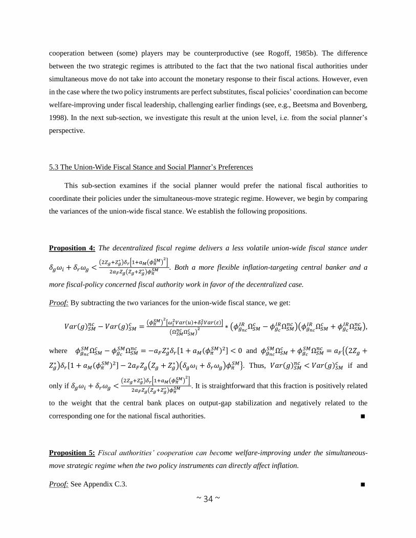
~ 34 ~

cooperation between (some) players may be counterproductive (see Rogoff, 1985b). The difference

between the two strategic regimes is attributed to the fact that the two national fiscal authorities under

simultaneous move do not take into account the monetary response to their fiscal actions. However, even

in the case where the two policy instruments are perfect substitutes, fiscal policies’ coordination can become

welfare-improving under fiscal leadership, challenging earlier findings (see, e.g., Beetsma and Bovenberg,

1998). In the next sub-section, we investigate this result at the union level, i.e. from the social planner’s

perspective.

5.3 The Union-Wide Fiscal Stance and Social Planner’s Preferences

This sub-section examines if the social planner would prefer the national fiscal authorities to

coordinate their policies under the simultaneous-move strategic regime. However, we begin by comparing

the variances of the union-wide fiscal stance. We establish the following propositions.

Proposition 4: The decentralized fiscal regime delivers a less volatile union-wide fiscal stance under

𝛿𝑔𝜔𝑖 + 𝛿𝑟𝜔𝑔 <(2𝑍𝑔+𝑍𝑔

∗ )𝛿𝑟[1+𝑎𝑀(𝜙𝜋𝑆𝑀)

2]

2𝑎𝐹𝑍𝑔(𝑍𝑔+𝑍𝑔∗ )𝜙𝜋

𝑆𝑀 . Both a more flexible inflation-targeting central banker and a

more fiscal-policy concerned fiscal authority work in favor of the decentralized case.

Proof: By subtracting the two variances for the union-wide fiscal stance, we get:

𝑉𝑎𝑟(𝑔)𝑆𝑀𝑛𝑐 − 𝑉𝑎𝑟(𝑔)𝑆𝑀

𝑐 =(𝜙𝜋

𝑆𝑀)2

[𝜔𝑖2𝑉𝑎𝑟(𝑢)+𝛿𝑟

2𝑉𝑎𝑟( )]

(Ω𝑆𝑀𝑛𝑐 Ω𝑆𝑀

𝑐 )2 ∗ (𝜙𝑔𝑛𝑐

𝐼𝑅 Ω𝑆𝑀𝑐 − 𝜙𝑔𝑐

𝐼𝑅Ω𝑆𝑀𝑛𝑐 )(𝜙𝑔𝑛𝑐

𝐼𝑅 Ω𝑆𝑀𝑐 + 𝜙𝑔𝑐

𝐼𝑅Ω𝑆𝑀𝑛𝑐 ),

where 𝜙𝑔𝑛𝑐𝑆𝑀 Ω𝑆𝑀

𝑐 − 𝜙𝑔𝑐𝑆𝑀Ω𝑆𝑀

𝑛𝑐 = −𝑎𝐹𝑍𝑔∗𝛿𝑟[1 + 𝑎𝑀(𝜙𝜋

𝑆𝑀)2] < 0 and 𝜙𝑔𝑛𝑐𝑆𝑀 Ω𝑆𝑀

𝑐 + 𝜙𝑔𝑐𝑆𝑀Ω𝑆𝑀

𝑛𝑐 = 𝑎𝐹{(2𝑍𝑔 +

𝑍𝑔∗)𝛿𝑟[1 + 𝑎𝑀(𝜙𝜋

𝑆𝑀)2] − 2𝑎𝐹𝑍𝑔(𝑍𝑔 + 𝑍𝑔∗)(𝛿𝑔𝜔𝑖 + 𝛿𝑟𝜔𝑔)𝜙𝜋

𝑆𝑀}. Thus, 𝑉𝑎𝑟(𝑔)𝑆𝑀𝑛𝑐 < 𝑉𝑎𝑟(𝑔)𝑆𝑀

𝑐 if and

only if 𝛿𝑔𝜔𝑖 + 𝛿𝑟𝜔𝑔 <(2𝑍𝑔+𝑍𝑔

∗ )𝛿𝑟[1+𝑎𝑀(𝜙𝜋𝑆𝑀)

2]

2𝑎𝐹𝑍𝑔(𝑍𝑔+𝑍𝑔∗ )𝜙𝜋

𝑆𝑀 . It is straightforward that this fraction is positively related

to the weight that the central bank places on output-gap stabilization and negatively related to the

corresponding one for the national fiscal authorities. ∎

Proposition 5: Fiscal authorities’ cooperation can become welfare-improving under the simultaneous-

move strategic regime when the two policy instruments can directly affect inflation.

Proof: See Appendix C.3. ∎

~ 35 ~

For the special case of perfect instrumental substitutability, the social planner prefers the national

fiscal authorities not to cooperate with one another. This result is consistent with Rogoff’s (1985b) classical

result that partial cooperation among (some) players is not welfare improving, whereas it is also consistent

with Beetsma and Bovenberg (1998). However, for the general case of 𝛿𝑔𝜔𝑖 + 𝛿𝑟𝜔𝑔 ≠ 0 we cannot get a

clear-cut result, which means that fiscal authorities’ cooperation after all can become welfare improving

when the two policy instruments can directly affect inflation, contradicting with the previous authors.

6. Comparison of the Alternative Strategic Regimes

This section is dedicated to a comparison of the alternative strategic regimes regarding union-wide

(cyclical) macroeconomic stabilization. In particular, we compare the variances of our main

macroeconomic variables, namely the output gap, inflation and the fiscal stance for the overall policy

coordination regime, the simultaneous-move one and the regime of fiscal leadership. We also consider both

fiscal regimes. We will see that the comparison mainly depends on a specific configuration of structural

parameters that shows which policy instrument is more effective in stabilizing aggregate demand relative

to inflation, namely 𝛿𝑔𝜔𝑖 + 𝛿𝑟𝜔𝑔.

6.1 The Simultaneous-Move Regime versus the Fiscal Leadership Regime

The comparisons of the variances of the main macroeconomic variables are presented in the Appendix

D.1. Our main results are as follows.

Proposition 6: Under perfect instrumental substitutability, the simultaneous-move strategic regime is

inferior to the fiscal leadership one under supply shocks, for both fiscal regimes (see, e.g., Dixit and

Lambertini, 2001). However, when we allow for the two policy instruments to directly affect inflation, the

simultaneous move can become a superior strategic regime, independent on shocks.

Proof: See Appendix D.2. ∎

Corollary 3: The common central bank unambiguously prefers the simultaneous-move strategic regime

over the fiscal leadership one under fiscal policies’ coordination, when 𝛿𝑔𝜔𝑖 + 𝛿𝑟𝜔𝑔 < 0.

~ 36 ~

Proof: In the Appendix D.1, we show that 𝑉𝑎𝑟(𝜋)𝑆𝑀𝑐 < 𝑉𝑎𝑟(𝜋)𝐹𝐿

𝑐 and 𝑉𝑎𝑟(𝑦)𝑆𝑀𝑐 < 𝑉𝑎𝑟(𝑦)𝐹𝐿

𝑐 for 𝛿𝑔𝜔𝑖 +

𝛿𝑟𝜔𝑔 < 0. Following the monetary authority’s expected loss, it is straightforward that 𝐸(𝐿𝑀)𝑆𝑀𝑐 <

𝐸(𝐿𝑀)𝐹𝐿𝑐 . The result is shock-independent. ∎

Corollary 3 shows that the simultaneous-move strategic regime can become superior to the fiscal

leadership strategic regime for pure cyclical macroeconomic stabilization at the union level if the national

fiscal authorities coordinate their policies. In fact, it shows that if fiscal policy can directly affect inflation

in a negative manner and fiscal policy is less efficient on aggregate demand than monetary policy, then this

is unambiguously so. This result contradicts with the famous result of Dixit and Lambertini (2001) for the

superiority of the leadership regimes over the simultaneous-move one.

6.2 The Overall Policy Coordination Regime versus the Fiscal Leadership for Coordinated Fiscal Policies

We have seen from our analysis so far that the two regimes are alike. For the special case of perfect

substitutability, we can determine three specific cases that refer to preferences where the fiscal leadership

regime for coordinated fiscal policies becomes superior.

Proposition 7: For the special case of perfect instrumental substitutability, the fiscal leadership regime

under fiscal authorities’ cooperation becomes unambiguously welfare-superior under three specific

circumstances regarding the agents’ (monetary authority, fiscal authorities, social planner) preference on

output-gap stabilization: (i) when all the authorities have the same preference, (ii) when the monetary and

the fiscal authorities jointly share society’s preferences and fiscal authorities’ preference is less than

double (as the fiscal authorities are two) from the monetary authority’s preference, and (ii) when the

monetary authority has society’s preference and at the same time the national fiscal authorities’ preference

is lower.

Proof: See Appendix D.3. ∎

7. Conclusion

We examine the policy mix in a monetary union in a strategic context when the two policy instruments

can directly affect inflation. In particular, we use a reduced-form two-country monetary union model based

~ 37 ~

on the New Keynesian framework, in order to study the strategic interactions of the monetary authority and

the national fiscal authorities under all strategic regimes and fiscal authorities’ cooperation. We find that

the cost channel of monetary policy limits union-wide demand shocks’ stabilization at the union level, that

the leader policy authority might choose not to trade-off its objectives, acting pro-cyclically, that fiscal

policy becomes non-neutral at the union level, and that fiscal authorities’ cooperation may end up welfare-

enhancing.

The most important result from our macroeconomic and welfare comparisons is that when we allow

the two policy instruments to directly affect inflation, then the choice of both the fiscal and the institutional

strategic regimes does matter at the union level, even when all the authorities have non-conflicting (but

different) objectives. Thus, the irrelevance conditions of Kempf and von Thadden (2013) and the symbiosis

result of Dixit and Lambertini (2001, 2003a) do not hold anymore. In particular, the monetary authority

becomes interested in the specific fiscal and strategic regimes. For the simultaneous-move strategic regime,

we succeed in defining the preferable fiscal regime for the monetary authority, depending on the

combination of parameters that show which policy instrument is more efficient in stabilizing aggregate

demand relative to inflation. We also find that the simultaneous-move strategic regime can become welfare-

improving. In particular, if fiscal policy can directly affect inflation negatively and at the same time fiscal

policy is less efficient in stabilizing aggregate demand (relative to inflation) than monetary policy, then the

common central bank prefers the simultaneous-move regime under fiscal authorities’ cooperation, as it

delivers less volatile union-wide inflation and output gap. Both results are of particular importance, as in

cases of extreme shocks and events, like the Great Recession, the simultaneous-move strategic regime

might be the most appropriate to analyse fiscal/monetary policy interactions (Dai and Sidiropoulos, 2011).

Empirical evidence provided by Hughes Hallett (2005) are also in favour of the simultaneous-move

strategic regime for the EMU.

In the special case that the two policy instruments are perfect substitutes in the stabilization process,

we have shown that (i) the alternative fiscal regimes do not matter, (ii) the simultaneous-move strategic

regime delivers exactly the same results with the monetary leadership regime at the union level for all

macroeconomic variables, which further means that both the common central bank and the social planner

are indifferent between those two strategic regimes, and (iii) that the simultaneous-move strategic regime

coincide with the fiscal leadership for inflation and the output gap, which makes the common central bank

indifferent between those two strategic regimes, but the union-wide fiscal stance is less volatile under fiscal

leadership, which makes this particular regime desirable for the social planner. We further show that for

common demand shocks, there is overall symbiosis between fiscal and monetary policies; i.e., all strategic

and fiscal regimes deliver the same equilibrium solutions for both union-wide and country-specific inflation

~ 38 ~

and output gap, which are also equal to the target (long-run equilibrium) values. For common supply shocks,

there is overall symbiosis only for the decentralized fiscal regime, but equilibrium solutions depart from

the target values. This resuts from the fiscal stance being both ain instrument and a target for the national

fiscal authorities (see Dixit and Lambertini, 2003a; Kempf and von Thadden, 2013). For the fiscal

leadership regime, the centralized fiscal regime delivers the same equilibrium solutions, too.

The similarity of the fiscal leadership regime under fiscal authorities’ cooperation with the overall

policy coordination regime means that the former regime enhances overall policy coordination (see, e.g.,

Andersen, 2008; Hughes Hallett and Weymark, 2007). In the special case of perfect instrumental

substitutability, where the two policy instruments are equally efficient, the union-wide fiscal stance is

equally volatile for both strategic regimes. Moreover, in this case, the fiscal leadership regime under

centralized fiscal policies delivers a less volatile union-wide inflation. As far as the social planner is

concerned, the fiscal leadership regime under fiscal authorities’ cooperation becomes unambiguously

welfare superior under three specific circumstances regarding the agents’ (monetary authority, fiscal

authorities, social planner) preference on output-gap stabilization: (i) when the monetary and the fiscal

authorities share the same preference, which also equals to the social planner’s preference, (ii) when the

monetary and the fiscal authorities jointly share society’s preferences and fiscal authorities’ preference is

less than double (as the fiscal authorities are two) of the monetary authority’s preference, and (ii) when the

monetary authority has the social planner’s preference and at the same time the national fiscal authorities’

preference is lower. In the second case, the overall policy coordination regime is desirable when fiscal

authorities’ preference is larger than double than the monetary authority’s preference, while the two regimes

are identical if the fiscal authorities’ preference is equal to the double of the monetary authority’s

preference.

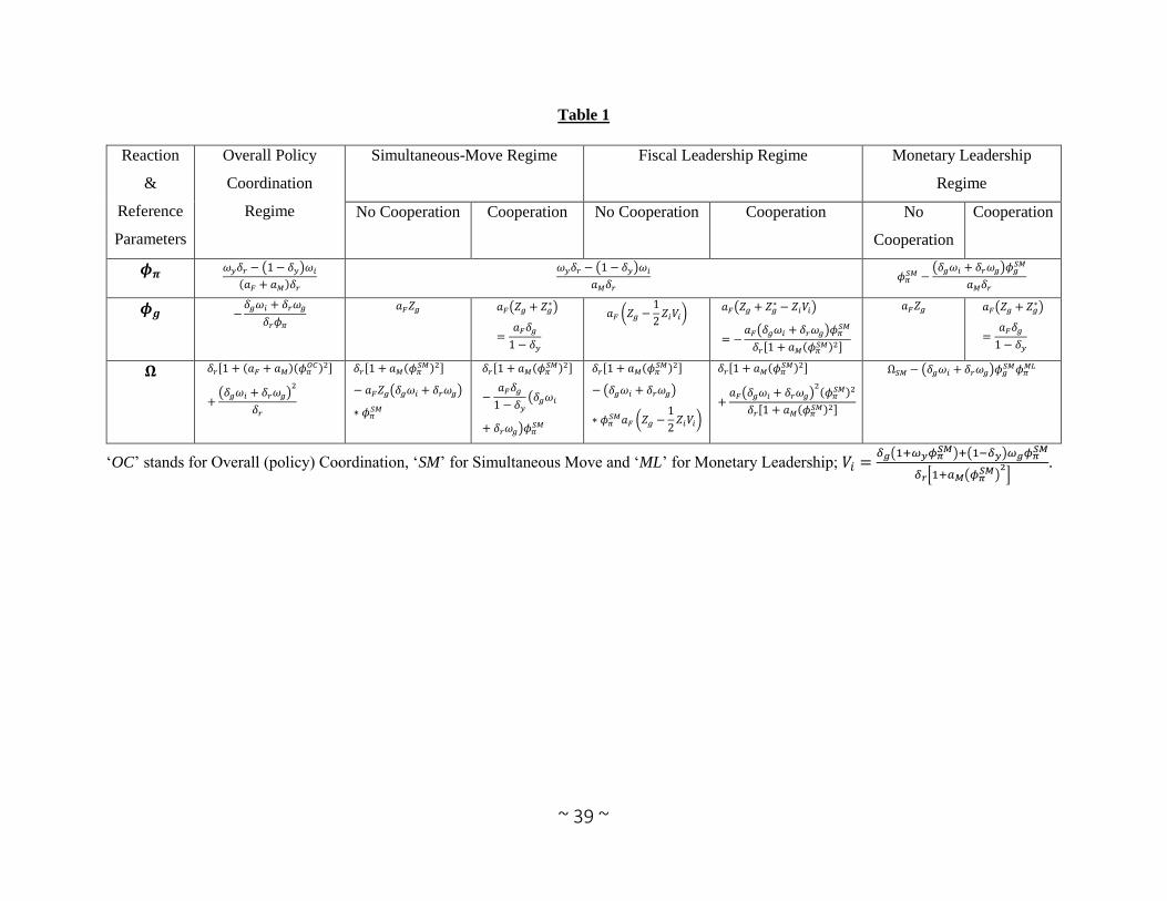
~ 39 ~

Table 1

Reaction

&

Reference

Parameters

Overall Policy

Coordination

Regime

Simultaneous-Move Regime Fiscal Leadership Regime Monetary Leadership

Regime

No Cooperation Cooperation No Cooperation Cooperation No

Cooperation

Cooperation

𝝓𝝅 𝜔𝑦𝛿𝑟 − (1 − 𝛿𝑦)𝜔𝑖

(𝑎𝐹 + 𝑎𝑀)𝛿𝑟

𝜔𝑦𝛿𝑟 − (1 − 𝛿𝑦)𝜔𝑖

𝑎𝑀𝛿𝑟

𝜙𝜋𝑆𝑀 −

(𝛿𝑔𝜔𝑖 + 𝛿𝑟𝜔𝑔)𝜙𝑔𝑆𝑀

𝑎𝑀𝛿𝑟

𝝓𝒈 −𝛿𝑔𝜔𝑖 + 𝛿𝑟𝜔𝑔

𝛿𝑟𝜙𝜋

𝑎𝐹𝑍𝑔 𝑎𝐹(𝑍𝑔 + 𝑍𝑔

∗)

=𝑎𝐹𝛿𝑔

1 − 𝛿𝑦

𝑎𝐹 (𝑍𝑔 −1

2𝑍𝑖𝑉𝑖)

𝑎𝐹(𝑍𝑔 + 𝑍𝑔∗ − 𝑍𝑖𝑉𝑖)

= −𝑎𝐹(𝛿𝑔𝜔𝑖 + 𝛿𝑟𝜔𝑔)𝜙𝜋

𝑆𝑀

𝛿𝑟[1 + 𝑎𝑀(𝜙𝜋𝑆𝑀)2]

𝑎𝐹𝑍𝑔 𝑎𝐹(𝑍𝑔 + 𝑍𝑔∗)

=𝑎𝐹𝛿𝑔

1 − 𝛿𝑦

𝛀 𝛿𝑟[1 + (𝑎𝐹 + 𝑎𝑀)(𝜙𝜋𝑂𝐶)2]

+(𝛿𝑔𝜔𝑖 + 𝛿𝑟𝜔𝑔)

2

𝛿𝑟

𝛿𝑟[1 + 𝑎𝑀(𝜙𝜋𝑆𝑀)2]

− 𝑎𝐹𝑍𝑔(𝛿𝑔𝜔𝑖 + 𝛿𝑟𝜔𝑔)

∗ 𝜙𝜋𝑆𝑀

𝛿𝑟[1 + 𝑎𝑀(𝜙𝜋𝑆𝑀)2]

−𝑎𝐹𝛿𝑔

1 − 𝛿𝑦

(𝛿𝑔𝜔𝑖

+ 𝛿𝑟𝜔𝑔)𝜙𝜋𝑆𝑀

𝛿𝑟[1 + 𝑎𝑀(𝜙𝜋𝑆𝑀)2]

− (𝛿𝑔𝜔𝑖 + 𝛿𝑟𝜔𝑔)

∗ 𝜙𝜋𝑆𝑀𝑎𝐹 (𝑍𝑔 −

1

2𝑍𝑖𝑉𝑖)

𝛿𝑟[1 + 𝑎𝑀(𝜙𝜋𝑆𝑀)2]

+𝑎𝐹(𝛿𝑔𝜔𝑖 + 𝛿𝑟𝜔𝑔)

2(𝜙𝜋

𝑆𝑀)2

𝛿𝑟[1 + 𝑎𝑀(𝜙𝜋𝑆𝑀)2]

Ω𝑆𝑀 − (𝛿𝑔𝜔𝑖 + 𝛿𝑟𝜔𝑔)𝜙𝑔𝑆𝑀𝜙𝜋

𝑀𝐿

‘OC’ stands for Overall (policy) Coordination, ‘SM’ for Simultaneous Move and ‘ML’ for Monetary Leadership; 𝑉𝑖 =𝛿𝑔(1+𝜔𝑦𝜙𝜋

𝑆𝑀)+(1−𝛿𝑦)𝜔𝑔𝜙𝜋𝑆𝑀

𝛿𝑟[1+𝑎𝑀(𝜙𝜋𝑆𝑀)

2]

.

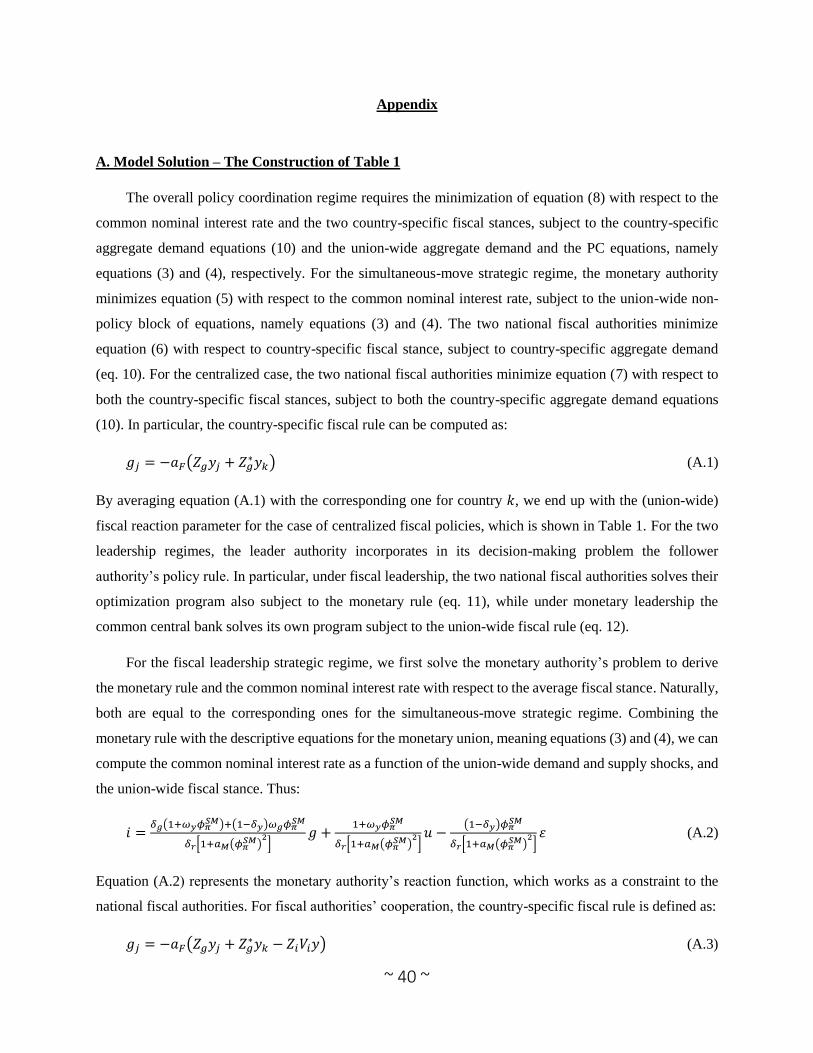
~ 40 ~

Appendix

A. Model Solution – The Construction of Table 1

The overall policy coordination regime requires the minimization of equation (8) with respect to the

common nominal interest rate and the two country-specific fiscal stances, subject to the country-specific

aggregate demand equations (10) and the union-wide aggregate demand and the PC equations, namely

equations (3) and (4), respectively. For the simultaneous-move strategic regime, the monetary authority

minimizes equation (5) with respect to the common nominal interest rate, subject to the union-wide non-

policy block of equations, namely equations (3) and (4). The two national fiscal authorities minimize

equation (6) with respect to country-specific fiscal stance, subject to country-specific aggregate demand

(eq. 10). For the centralized case, the two national fiscal authorities minimize equation (7) with respect to

both the country-specific fiscal stances, subject to both the country-specific aggregate demand equations

(10). In particular, the country-specific fiscal rule can be computed as:

𝑔𝑗 = −𝑎𝐹(𝑍𝑔𝑦𝑗 + 𝑍𝑔∗𝑦𝑘) (A.1)

By averaging equation (A.1) with the corresponding one for country 𝑘, we end up with the (union-wide)

fiscal reaction parameter for the case of centralized fiscal policies, which is shown in Table 1. For the two

leadership regimes, the leader authority incorporates in its decision-making problem the follower

authority’s policy rule. In particular, under fiscal leadership, the two national fiscal authorities solves their

optimization program also subject to the monetary rule (eq. 11), while under monetary leadership the

common central bank solves its own program subject to the union-wide fiscal rule (eq. 12).

For the fiscal leadership strategic regime, we first solve the monetary authority’s problem to derive

the monetary rule and the common nominal interest rate with respect to the average fiscal stance. Naturally,

both are equal to the corresponding ones for the simultaneous-move strategic regime. Combining the

monetary rule with the descriptive equations for the monetary union, meaning equations (3) and (4), we can

compute the common nominal interest rate as a function of the union-wide demand and supply shocks, and

the union-wide fiscal stance. Thus:

𝑖 =𝛿𝑔(1+𝜔𝑦𝜙𝜋

𝑆𝑀)+(1−𝛿𝑦)𝜔𝑔𝜙𝜋𝑆𝑀

𝛿𝑟[1+𝑎𝑀(𝜙𝜋𝑆𝑀)

2]

𝑔 +1+𝜔𝑦𝜙𝜋

𝑆𝑀

𝛿𝑟[1+𝑎𝑀(𝜙𝜋𝑆𝑀)

2]𝑢 −

(1−𝛿𝑦)𝜙𝜋𝑆𝑀

𝛿𝑟[1+𝑎𝑀(𝜙𝜋𝑆𝑀)

2]휀 (A.2)

Equation (A.2) represents the monetary authority’s reaction function, which works as a constraint to the

national fiscal authorities. For fiscal authorities’ cooperation, the country-specific fiscal rule is defined as:

𝑔𝑗 = −𝑎𝐹(𝑍𝑔𝑦𝑗 + 𝑍𝑔∗𝑦𝑘 − 𝑍𝑖𝑉𝑖𝑦) (A.3)

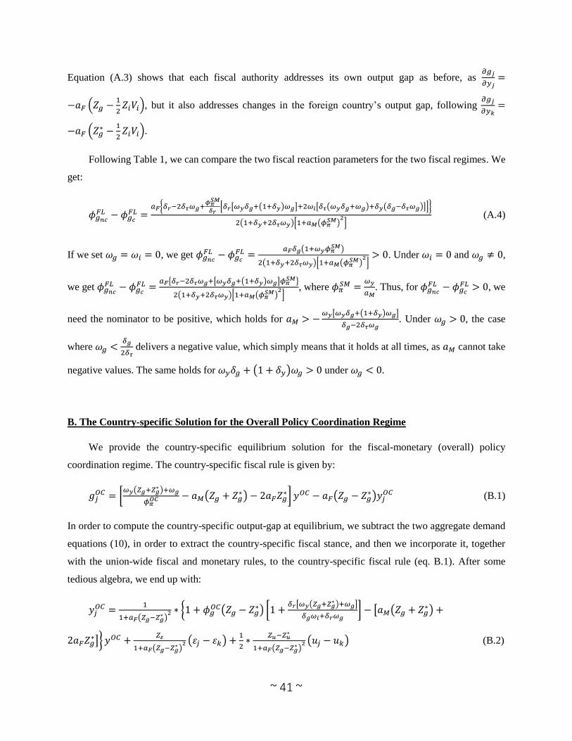
~ 41 ~

Equation (A.3) shows that each fiscal authority addresses its own output gap as before, as 𝜕𝑔𝑗

𝜕𝑦𝑗=

−𝑎𝐹 (𝑍𝑔 −1

2𝑍𝑖𝑉𝑖), but it also addresses changes in the foreign country’s output gap, following

𝜕𝑔𝑗

𝜕𝑦𝑘=

−𝑎𝐹 (𝑍𝑔∗ −

1

2𝑍𝑖𝑉𝑖).

Following Table 1, we can compare the two fiscal reaction parameters for the two fiscal regimes. We

get:

𝜙𝑔𝑛𝑐𝐹𝐿 − 𝜙𝑔𝑐

𝐹𝐿 =𝑎𝐹{𝛿𝑟−2𝛿𝜏𝜔𝑔+

𝜙𝜋𝑆𝑀

𝛿𝑟[𝛿𝑟[𝜔𝑦𝛿𝑔+(1+𝛿𝑦)𝜔𝑔]+2𝜔𝑖[𝛿𝜏(𝜔𝑦𝛿𝑔+𝜔𝑔)+𝛿𝑦(𝛿𝑔−𝛿𝜏𝜔𝑔)]]}

2(1+𝛿𝑦+2𝛿𝜏𝜔𝑦)[1+𝑎𝑀(𝜙𝜋𝑆𝑀)

2]

(A.4)

If we set 𝜔𝑔 = 𝜔𝑖 = 0, we get 𝜙𝑔𝑛𝑐𝐹𝐿 − 𝜙𝑔𝑐

𝐹𝐿 =𝑎𝐹𝛿𝑔(1+𝜔𝑦𝜙𝜋

𝑆𝑀)

2(1+𝛿𝑦+2𝛿𝜏𝜔𝑦)[1+𝑎𝑀(𝜙𝜋𝑆𝑀)

2]

> 0. Under 𝜔𝑖 = 0 and 𝜔𝑔 ≠ 0,

we get 𝜙𝑔𝑛𝑐𝐹𝐿 − 𝜙𝑔𝑐

𝐹𝐿 =𝑎𝐹{𝛿𝑟−2𝛿𝜏𝜔𝑔+[𝜔𝑦𝛿𝑔+(1+𝛿𝑦)𝜔𝑔]𝜙𝜋

𝑆𝑀}

2(1+𝛿𝑦+2𝛿𝜏𝜔𝑦)[1+𝑎𝑀(𝜙𝜋𝑆𝑀)

2]

, where 𝜙𝜋𝑆𝑀 =

𝜔𝑦

𝑎𝑀. Thus, for 𝜙𝑔𝑛𝑐

𝐹𝐿 − 𝜙𝑔𝑐𝐹𝐿 > 0, we

need the nominator to be positive, which holds for 𝑎𝑀 > −𝜔𝑦[𝜔𝑦𝛿𝑔+(1+𝛿𝑦)𝜔𝑔]

𝛿𝑔−2𝛿𝜏𝜔𝑔. Under 𝜔𝑔 > 0, the case

where 𝜔𝑔 <𝛿𝑔

2𝛿𝜏 delivers a negative value, which simply means that it holds at all times, as 𝑎𝑀 cannot take

negative values. The same holds for 𝜔𝑦𝛿𝑔 + (1 + 𝛿𝑦)𝜔𝑔 > 0 under 𝜔𝑔 < 0.

B. The Country-specific Solution for the Overall Policy Coordination Regime

We provide the country-specific equilibrium solution for the fiscal-monetary (overall) policy

coordination regime. The country-specific fiscal rule is given by:

𝑔𝑗𝑂𝐶 = [

𝜔𝑦(𝑍𝑔+𝑍𝑔∗ )+𝜔𝑔

𝜙𝜋𝑂𝐶 − 𝑎𝑀(𝑍𝑔 + 𝑍𝑔

∗) − 2𝑎𝐹𝑍𝑔∗] 𝑦𝑂𝐶 − 𝑎𝐹(𝑍𝑔 − 𝑍𝑔

∗)𝑦𝑗𝑂𝐶 (B.1)

In order to compute the country-specific output-gap at equilibrium, we subtract the two aggregate demand

equations (10), in order to extract the country-specific fiscal stance, and then we incorporate it, together

with the union-wide fiscal and monetary rules, to the country-specific fiscal rule (eq. B.1). After some

tedious algebra, we end up with:

𝑦𝑗𝑂𝐶 =

1

1+𝑎𝐹(𝑍𝑔−𝑍𝑔∗ )

2 ∗ {1 + 𝜙𝑔𝑂𝐶(𝑍𝑔 − 𝑍𝑔

∗) [1 +𝛿𝑟[𝜔𝑦(𝑍𝑔+𝑍𝑔

∗ )+𝜔𝑔]

𝛿𝑔𝜔𝑖+𝛿𝑟𝜔𝑔] − [𝑎𝑀(𝑍𝑔 + 𝑍𝑔

∗) +

2𝑎𝐹𝑍𝑔∗]} 𝑦𝑂𝐶 +

𝑍

1+𝑎𝐹(𝑍𝑔−𝑍𝑔∗ )

2 (휀𝑗 − 휀𝑘) +1

2∗

𝑍𝑢−𝑍𝑢∗

1+𝑎𝐹(𝑍𝑔−𝑍𝑔∗ )

2 (𝑢𝑗 − 𝑢𝑘) (B.2)

~ 42 ~

At equilibrium, we incorporate the solution for the union-wide output gap following equation (16).

C. A Welfare Analysis of the Alternative Fiscal Regimes (Section 5)

C.1 The Monetary Authority’s Welfare Analysis (Section 5.1)

We compare the variances for union-wide inflation and the output gap. We get:

𝑉𝑎𝑟(𝜋)𝐼𝑅𝑛𝑐 − 𝑉𝑎𝑟(𝜋)𝐼𝑅

𝑐 =𝜔𝑖

2𝑉𝑎𝑟(𝑢)+𝛿𝑟2𝑉𝑎𝑟( )

(Ω𝐼𝑅𝑛𝑐Ω𝐼𝑅

𝑐 )2 ∗ (Ω𝐼𝑅

𝑐 − Ω𝐼𝑅𝑛𝑐)(Ω𝐼𝑅

𝑐 + Ω𝐼𝑅𝑛𝑐) (C.1)

𝑉𝑎𝑟(𝑦)𝐼𝑅𝑛𝑐 − 𝑉𝑎𝑟(𝑦)𝐼𝑅

𝑐 = (𝜙𝜋𝐼𝑅)2[𝑉𝑎𝑟(𝜋)𝐼𝑅

𝑛𝑐 − 𝑉𝑎𝑟(𝜋)𝐼𝑅𝑐 ], (C.2)

where ‘IR’ stands for ‘Institutional Regimes’. The former equation holds for all strategic regimes, while the

latter holds only for the simultaneous move and the fiscal leadership regimes. For the monetary leadership

regime, it becomes:

𝑉𝑎𝑟(𝑦)𝑀𝐿𝑛𝑐 − 𝑉𝑎𝑟(𝑦)𝑀𝐿

𝑐 =𝜔𝑖

2𝑉𝑎𝑟(𝑢)+𝛿𝑟2𝑉𝑎𝑟( )

(Ω𝑀𝐿𝑛𝑐 Ω𝑀𝐿

𝑐 )2 ∗ (𝜙𝜋𝑛𝑐

𝑀𝐿 Ω𝑀𝐿𝑐 − 𝜙𝜋𝑐

𝑀𝐿Ω𝑀𝐿𝑛𝑐 )(𝜙𝜋𝑛𝑐

𝑀𝐿 Ω𝑀𝐿𝑐 + 𝜙𝜋𝑐

𝑀𝐿Ω𝑀𝐿𝑛𝑐 ) (C.3)

We can compare the monetary authority’s loss under the two alternative fiscal regimes for the simultaneous

move and the fiscal leadership regime. It is straightforward that:

𝐸(𝐿𝑀)𝐼𝑅𝑛𝑐 − 𝐸(𝐿𝑀)𝐼𝑅

𝑐 =1

2∗ [1 + 𝑎𝑀(𝜙𝜋

𝐼𝑅)2] ∗ [𝑉𝑎𝑟(𝜋)𝐼𝑅𝑛𝑐 − 𝑉𝑎𝑟(𝜋)𝐼𝑅

𝑐 ] (C.4)

The reaction and the reference parameters for both fiscal regimes are taken from Table 1.

C.2. Proof of Proposition 3

For the simultaneous-move strategic regime, we get:

𝐸 (𝐿𝐹𝑗)

𝑆𝑀

𝑛𝑐− 𝐸 (𝐿𝐹𝑗

)𝑆𝑀

𝑐=

1

2∗

𝑎𝐹(𝜙𝜋𝑆𝑀)

2(𝜔𝑖

2𝜎𝑢2+𝛿𝑟

2𝜎2)

(Ω𝑆𝑀𝑛𝑐 Ω𝑆𝑀

𝑐 )2

[1+𝑎𝐹(𝑍𝑔−𝑍𝑔∗ )

2]

2 ∗ {(1 + 𝑎𝐹𝑍𝑔2) [1 + 𝑎𝐹(𝑍𝑔 −

𝑍𝑔∗)

2]

2(Ω𝑆𝑀

𝑐 )2 − [1 + 𝑎𝐹(𝑍𝑔 + 𝑍𝑔∗)

2] [1 + 𝑎𝐹𝑍𝑔(𝑍𝑔 − 𝑍𝑔

∗)]2

(Ω𝑆𝑀𝑛𝑐 )2},

~ 43 ~

where we can get a clear-cut result for 𝛿𝑔𝜔𝑖 + 𝛿𝑟𝜔𝑔 = 0, where 𝐸 (𝐿𝐹𝑗)

𝑆𝑀

𝑛𝑐− 𝐸 (𝐿𝐹𝑗

)𝑆𝑀

𝑐= −

1

2∗

𝑎𝐹2𝑍𝑔

∗ (𝜙𝜋𝑆𝑀)

2(𝜔𝑖

2𝜎𝑢2+𝛿𝑟

2𝜎2)

𝛿𝑟[1+𝑎𝑀(𝜙𝜋𝑆𝑀)

2][1+𝑎𝐹(𝑍𝑔−𝑍𝑔

∗ )2

]2 ∗ {(𝑍𝑔 − 𝑍𝑔

∗)[2 + 𝑎𝐹(𝑍𝑔 − 𝑍𝑔∗)(2𝑍𝑔 + 𝑍𝑔

∗)] + (2𝑍𝑔 + 𝑍𝑔∗)[1 +

𝑎𝐹𝑍𝑔(𝑍𝑔 − 𝑍𝑔∗)]

2} < 0, as 𝑍𝑔 − 𝑍𝑔

∗ > 0. For the fiscal leadership regime, we get:

𝐸 (𝐿𝐹𝑗)

𝐹𝐿

𝑛𝑐− 𝐸 (𝐿𝐹𝑗

)𝐹𝐿

𝑐=

1

2∗

(𝜙𝜋𝑆𝑀)

2(𝜔𝑖

2𝜎𝑢2+𝛿𝑟

2𝜎2)

(Ω𝐹𝐿𝑛𝑐Ω𝐹𝐿

𝑐 )2 ∗ {𝑎𝐹(Ω𝐹𝐿

𝑐 − Ω𝐹𝐿𝑛𝑐)(Ω𝐹𝐿

𝑐 + Ω𝐹𝐿𝑛𝑐) + (𝜙𝑔𝑛𝑐

𝐹𝐿 Ω𝐹𝐿𝑐 −

𝜙𝑔𝑐𝐹𝐿Ω𝐹𝐿

𝑛𝑐)(𝜙𝑔𝑛𝑐𝐹𝐿 Ω𝐹𝐿

𝑐 + 𝜙𝑔𝑐𝐹𝐿Ω𝐹𝐿

𝑛𝑐)},

where we already know Ω𝐹𝐿𝑐 − Ω𝐹𝐿

𝑛𝑐 and Ω𝐹𝐿𝑐 + Ω𝐹𝐿

𝑛𝑐 from the Proof of Proposition 2. Moreover, 𝜙𝑔𝑛𝑐𝐹𝐿 Ω𝐹𝐿

𝑐 −

𝜙𝑔𝑐𝐹𝐿Ω𝐹𝐿

𝑛𝑐 = −𝑎𝐹 (𝑍𝑔∗ −

1

2𝑍𝑖𝑉𝑖) 𝛿𝑟[1 + 𝑎𝑀(𝜙𝜋

𝑆𝑀)2] and 𝜙𝑔𝑛𝑐𝐹𝐿 Ω𝐹𝐿

𝑐 + 𝜙𝑔𝑐𝐹𝐿Ω𝐹𝐿

𝑛𝑐 = 𝑎𝐹 {2 (𝑍𝑔 −1

2𝑍𝑖𝑉𝑖) Ω𝐹𝐿

𝑐 +

(𝑍𝑔∗ −

1

2𝑍𝑖𝑉𝑖) 𝛿𝑟[1 + 𝑎𝑀(𝜙𝜋

𝑆𝑀)2]}. We can see that we can only get an unambiguous result for both

(𝛿𝑔𝜔𝑖 + 𝛿𝑟𝜔𝑔) (𝑍𝑔∗ −

1

2𝑍𝑖𝑉𝑖) > 0 and (𝑍𝑔 −

1

2𝑍𝑖𝑉𝑖) (𝑍𝑔

∗ −1

2𝑍𝑖𝑉𝑖) > 0, where 𝐸 (𝐿𝐹𝑗

)𝐹𝐿

𝑛𝑐< 𝐸 (𝐿𝐹𝑗

)𝐹𝐿

𝑐.

Thus, for the special case of 𝛿𝑔𝜔𝑖 + 𝛿𝑟𝜔𝑔 = 0, we need (𝑍𝑔 −1

2𝑍𝑖𝑉𝑖) (𝑍𝑔

∗ −1

2𝑍𝑖𝑉𝑖) > 0. ∎

C.3. Proof of Proposition 5

For both the simultaneous move and the fiscal leadership regime, we compare society’s loss under the

two alternative fiscal regimes, as:

𝐸(𝐿𝑆)𝐼𝑅𝑛𝑐 − 𝐸(𝐿𝑆)𝐼𝑅

𝑐 =1

2∗

𝜔𝑖2𝑉𝑎𝑟(𝑢)+𝛿𝑟

2𝑉𝑎𝑟( )

(Ω𝐼𝑅𝑛𝑐Ω𝐼𝑅

𝑐 )2 ∗ {[1 + 𝑎𝑆(𝜙𝜋

𝑆𝑀)2](Ω𝐼𝑅𝑐 − Ω𝐼𝑅

𝑛𝑐)(Ω𝐼𝑅𝑐 + Ω𝐼𝑅

𝑛𝑐) +

𝑏𝑆(𝜙𝜋𝑆𝑀)2(𝜙𝑔𝑛𝑐

𝐼𝑅 Ω𝐼𝑅𝑐 − 𝜙𝑔𝑐

𝐼𝑅Ω𝐼𝑅𝑛𝑐)(𝜙𝑔𝑛𝑐

𝐼𝑅 Ω𝐼𝑅𝑐 + 𝜙𝑔𝑐

𝐼𝑅Ω𝐼𝑅𝑛𝑐)}

For the simultaneous-move strategic regime, we get:

𝐸(𝐿𝑆)𝑆𝑀𝑛𝑐 − 𝐸(𝐿𝑆)𝑆𝑀

𝑐 = −1

2∗

𝑎𝐹𝑍𝑔∗ 𝜙𝜋

𝑆𝑀[𝜔𝑖2𝑉𝑎𝑟(𝑢)+𝛿𝑟

2𝑉𝑎𝑟( )]

(Ω𝑆𝑀𝑛𝑐 Ω𝑆𝑀

𝑐 )2 ∗ {𝑎𝐹(2𝑍𝑔 + 𝑍𝑔

∗)𝜙𝜋𝑆𝑀 ∗ [𝑏𝑆𝛿𝑟

2(1 +

𝑎𝑀(𝜙𝜋𝑆𝑀)2)2 − (𝛿𝑔𝜔𝑖 + 𝛿𝑟𝜔𝑔)

2(1 + 𝑎𝑆(𝜙𝜋

𝑆𝑀)2)2] + 2𝛿𝑟[1 + 𝑎𝑀(𝜙𝜋𝑆𝑀)2](𝛿𝑔𝜔𝑖 + 𝛿𝑟𝜔𝑔) ∗ [1 +

𝑎𝑆(𝜙𝜋𝑆𝑀)2 − 𝑏𝑆𝑎𝐹

2𝑍𝑔(𝑍𝑔 + 𝑍𝑔∗)(𝜙𝜋

𝑆𝑀)2]} ≷ 0

For the special case of 𝛿𝑔𝜔𝑖 + 𝛿𝑟𝜔𝑔 = 0, we get:

𝐸(𝐿𝑆)𝑆𝑀𝑛𝑐 − 𝐸(𝐿𝑆)𝑆𝑀

𝑐 = −1

2∗

𝑏𝑆𝑎𝐹2𝑍𝑔

∗ (2𝑍𝑔+𝑍𝑔∗ )𝛿𝑟

2(𝜙𝜋𝑆𝑀)

2[1+𝑎𝑀(𝜙𝜋

𝑆𝑀)2

]2

[𝜔𝑖2𝑉𝑎𝑟(𝑢)+𝛿𝑟

2𝑉𝑎𝑟( )]

(Ω𝑆𝑀𝑛𝑐 Ω𝑆𝑀

𝑐 )2 < 0 ∎

~ 44 ~

D. Comparison of the Alternative Strategic Regimes (Section 6)

D.1. The Simultaneous-Move versus the Fiscal Leadership Regime

We compare the union-wide inflation rate and the output gap, following equilibrium solutions

(equations 15 and 16). We get:

𝑉𝑎𝑟(𝜋)𝑆𝑀 − 𝑉𝑎𝑟(𝜋)𝐹𝐿 =𝜔𝑖

2𝑉𝑎𝑟(𝑢)+𝛿𝑟2𝑉𝑎𝑟( )

(Ω𝑆𝑀Ω𝐹𝐿)2 ∗ (Ω𝐹𝐿 − Ω𝑆𝑀)(Ω𝐹𝐿 + Ω𝑆𝑀) (D.1)

𝑉𝑎𝑟(𝑦)𝑆𝑀 − 𝑉𝑎𝑟(𝑦)𝐹𝐿 = (𝜙𝜋𝑆𝑀)2[𝑉𝑎𝑟(𝜋)𝑆𝑀 − 𝑉𝑎𝑟(𝜋)𝐹𝐿], (D.2)

where Ω𝐹𝐿 − Ω𝑆𝑀 = (𝛿𝑔𝜔𝑖 + 𝛿𝑟𝜔𝑔)𝜙𝜋𝑆𝑀(𝜙𝑔

𝑆𝑀 − 𝜙𝑔𝐹𝐿) and Ω𝐹𝐿 + Ω𝑆𝑀 = 2𝛿𝑟[1 + 𝑎𝑀(𝜙𝜋

𝑆𝑀)2] −

(𝛿𝑔𝜔𝑖 + 𝛿𝑟𝜔𝑔)𝜙𝜋𝑆𝑀(𝜙𝑔

𝑆𝑀 + 𝜙𝑔𝐹𝐿). For the two fiscal regimes, we get:

𝑉𝑎𝑟(𝜋)𝑆𝑀𝑛𝑐 − 𝑉𝑎𝑟(𝜋)𝐹𝐿

𝑛𝑐 =𝜔𝑖

2𝑉𝑎𝑟(𝑢)+𝛿𝑟2𝑉𝑎𝑟( )

(Ω𝑆𝑀𝑛𝑐 Ω𝐹𝐿

𝑛𝑐)2 𝑎𝐹𝑍𝑖𝑉𝑖𝜙𝜋

𝑆𝑀(𝛿𝑔𝜔𝑖 + 𝛿𝑟𝜔𝑔) {𝛿𝑟[1 + 𝑎𝑀(𝜙𝜋𝑆𝑀)2] −

(𝛿𝑔𝜔𝑖 + 𝛿𝑟𝜔𝑔)𝜙𝜋𝑆𝑀𝑎𝐹 (𝑍𝑔 −

1

4𝑍𝑖𝑉𝑖)} (D.3)

𝑉𝑎𝑟(𝜋)𝑆𝑀𝑐 − 𝑉𝑎𝑟(𝜋)𝐹𝐿

𝑐 =𝜔𝑖

2𝑉𝑎𝑟(𝑢)+𝛿𝑟2𝑉𝑎𝑟( )

(Ω𝑆𝑀𝑐 Ω𝐹𝐿

𝑐 )2 𝑎𝐹𝑍𝑖𝑉𝑖𝜙𝜋

𝑆𝑀(𝛿𝑔𝜔𝑖 + 𝛿𝑟𝜔𝑔){𝛿𝑟[1 + 𝑎𝑀(𝜙𝜋𝑆𝑀)2] −

(𝛿𝑔𝜔𝑖 + 𝛿𝑟𝜔𝑔)𝜙𝜋𝑆𝑀𝑎𝐹[2(𝑍𝑔 + 𝑍𝑔

∗) − 𝑍𝑖𝑉𝑖]} (D.4)

Both equations (D.3) and (D.4) reveal that in the special case of 𝛿𝑔𝜔𝑖 + 𝛿𝑟𝜔𝑔 = 0, then 𝑉𝑎𝑟(𝜋)𝑆𝑀 =

𝑉𝑎𝑟(𝜋)𝐹𝐿 and 𝑉𝑎𝑟(𝑦)𝑆𝑀 = 𝑉𝑎𝑟(𝑦)𝐹𝐿. Following equation (D.3), under 𝛿𝑔𝜔𝑖 + 𝛿𝑟𝜔𝑔 > 0 and 𝑍𝑔 −

1

4𝑍𝑖𝑉𝑖 < 0, then 𝑉𝑎𝑟(𝜋)𝑆𝑀

𝑛𝑐 > 𝑉𝑎𝑟(𝜋)𝐹𝐿𝑛𝑐, and vice versa. Following equation (D.4) for the cooperative

fiscal regime, under 𝛿𝑔𝜔𝑖 + 𝛿𝑟𝜔𝑔 > 0 and 2(𝑍𝑔 + 𝑍𝑔∗) − 𝑍𝑖𝑉𝑖 < 0, then 𝑉𝑎𝑟(𝜋)𝑆𝑀

𝑐 > 𝑉𝑎𝑟(𝜋)𝐹𝐿𝑐 .

However, under 𝛿𝑔𝜔𝑖 + 𝛿𝑟𝜔𝑔 < 0 then 2(𝑍𝑔 + 𝑍𝑔∗) − 𝑍𝑖𝑉𝑖 =

𝛿𝑔

1−𝛿𝑦−

(𝛿𝑔𝜔𝑖+𝛿𝑟𝜔𝑔)𝜙𝜋𝑆𝑀

𝛿𝑟[1+𝑎𝑀(𝜙𝜋𝑆𝑀)

2]

> 0. This means

that 𝑉𝑎𝑟(𝜋)𝑆𝑀𝑐 < 𝑉𝑎𝑟(𝜋)𝐹𝐿

𝑐 , hence 𝑉𝑎𝑟(𝑦)𝑆𝑀𝑐 < 𝑉𝑎𝑟(𝑦)𝐹𝐿

𝑐 .

Turning now to the union-wide fiscal stance, we get:

𝑉𝑎𝑟(𝑔)𝑆𝑀 − 𝑉𝑎𝑟(𝑔)𝐹𝐿 =(𝜙𝜋

𝑆𝑀)2

[𝜔𝑖2𝑉𝑎𝑟(𝑢)+𝛿𝑟

2𝑉𝑎𝑟( )]

(Ω𝑆𝑀Ω𝐹𝐿)2 (𝜙𝑔𝑆𝑀Ω𝐹𝐿 − 𝜙𝑔

𝐹𝐿Ω𝐹𝐿)(𝜙𝑔𝑆𝑀Ω𝐹𝐿 + 𝜙𝑔

𝐹𝐿Ω𝐹𝐿),

(D.5)

For the decentralized fiscal regime, 𝜙𝑔𝑛𝑐𝑆𝑀 Ω𝐹𝐿

𝑛𝑐 − 𝜙𝑔𝑛𝑐𝐹𝐿 Ω𝑆𝑀

𝑛𝑐 =1

2𝑎𝐹𝛿𝑟𝑍𝑖𝑉𝑖[1 + 𝑎𝑀(𝜙𝜋

𝑆𝑀)2] > 0 and

𝜙𝑔𝑛𝑐𝑆𝑀 Ω𝐹𝐿

𝑛𝑐 + 𝜙𝑔𝑛𝑐𝐹𝐿 Ω𝑆𝑀

𝑛𝑐 = 𝑎𝐹 {(2𝑍𝑔 −1

2𝑍𝑖𝑉𝑖) 𝛿𝑟[1 + 𝑎𝑀(𝜙𝜋

𝑆𝑀)2] − 2(𝛿𝑔𝜔𝑖 + 𝛿𝑟𝜔𝑔)𝜙𝜋𝑆𝑀𝑎𝐹𝑍𝑔 (𝑍𝑔 −

~ 45 ~

1

2𝑍𝑖𝑉𝑖)}. Thus, under 𝛿𝑔𝜔𝑖 + 𝛿𝑟𝜔𝑔 = 0, then 𝑠𝑖𝑔𝑛{𝑉𝑎𝑟(𝑔)𝑆𝑀

𝑛𝑐 − 𝑉𝑎𝑟(𝑔)𝐹𝐿𝑛𝑐} = 𝑠𝑖𝑔𝑛 {2𝑍𝑔 −

1

2𝑍𝑖𝑉𝑖},

which is unambiguously positive for 𝜔𝑔 = 𝜔𝑖 = 0. For 𝑉𝑎𝑟(𝑔)𝑆𝑀𝑛𝑐 > 𝑉𝑎𝑟(𝑔)𝐹𝐿

𝑛𝑐 we need either 𝑍𝑔 −

1

2𝑍𝑖𝑉𝑖 > 0 or 𝑍𝑔 −

1

2𝑍𝑖𝑉𝑖 < 0 and 2𝑍𝑔 −

1

2𝑍𝑖𝑉𝑖 < 0 for 𝛿𝑔𝜔𝑖 + 𝛿𝑟𝜔𝑔 < 0, and both 𝑍𝑔 −

1

2𝑍𝑖𝑉𝑖 < 0 and

2𝑍𝑔 −1

2𝑍𝑖𝑉𝑖 > 0 for 𝛿𝑔𝜔𝑖 + 𝛿𝑟𝜔𝑔 > 0. For the centralized fiscal regime, we have 𝜙𝑔𝑐

𝑆𝑀Ω𝐹𝐿𝑐 − 𝜙𝑔𝑐

𝐹𝐿Ω𝑆𝑀𝑐 =

𝑎𝐹𝛿𝑟𝑍𝑖𝑉𝑖[1 + 𝑎𝑀(𝜙𝜋𝑆𝑀)2] > 0 and 𝜙𝑔𝑐

𝑆𝑀Ω𝐹𝐿𝑐 + 𝜙𝑔𝑐

𝐹𝐿Ω𝑆𝑀𝑐 = 𝑎𝐹 {[2(𝑍𝑔 + 𝑍𝑔

∗) − 𝑍𝑖𝑉𝑖]𝛿𝑟[1 + 𝑎𝑀(𝜙𝜋𝑆𝑀)2] +

2𝜙𝑔𝑐𝑆𝑀(𝛿𝑔𝜔𝑖 + 𝛿𝑟𝜔𝑔)

2(𝜙𝜋

𝑆𝑀)2}. We can get a clear-cut result for 𝛿𝑔𝜔𝑖 + 𝛿𝑟𝜔𝑔 < 0, where 2𝑍𝑔 + 2𝑍𝑔∗ −

𝑍𝑖𝑉𝑖 > 0, hence 𝑉𝑎𝑟(𝑔)𝑆𝑀𝑐 > 𝑉𝑎𝑟(𝑔)𝐹𝐿

𝑐 . In the special case of 𝛿𝑔𝜔𝑖 + 𝛿𝑟𝜔𝑔 = 0, then 𝜙𝑔𝑐𝑆𝑀Ω𝐹𝐿

𝑐 +

𝜙𝑔𝑐𝐹𝐿Ω𝑆𝑀

𝑐 =𝑎𝐹𝛿𝑔𝛿𝑟[1+𝑎𝑀(𝜙𝜋

𝑆𝑀)2

]

1−𝛿𝑦> 0, which again leads to 𝑉𝑎𝑟(𝑔)𝑆𝑀

𝑐 > 𝑉𝑎𝑟(𝑔)𝐹𝐿𝑐 .

D.2. Proof of Proposition 6

The social planner’s expected loss can be computed from equation (9) as:

𝐸(𝐿𝑆) =1

2∗

1+(𝑎𝑆+𝑏𝑆𝜙𝑔2)𝜙𝜋

2

Ω2 ∗ [𝜔𝑖2𝑉𝑎𝑟(𝑢) + 𝛿𝑟

2𝑉𝑎𝑟(휀)]

We compare the expected losses for the two strategic regimes, as:

𝐸(𝐿𝑆)𝑆𝑀 − 𝐸(𝐿𝑆)𝐹𝐿 =1

2∗

𝜔𝑖2𝑉𝑎𝑟(𝑢)+𝛿𝑟

2𝑉𝑎𝑟( )

(Ω𝑆𝑀Ω𝐹𝐿)2 ∗ {[1 + 𝑎𝑆(𝜙𝜋𝑆𝑀)2](Ω𝐹𝐿 − Ω𝑆𝑀)(𝛺𝐹𝐿 + 𝛺𝑆𝑀) +

𝑏𝑆(𝜙𝜋𝑆𝑀)2(𝜙𝑔

𝑆𝑀Ω𝐹𝐿 − 𝜙𝑔𝐹𝐿Ω𝑆𝑀)(𝜙𝑔

𝑆𝑀𝛺𝐹𝐿 − 𝜙𝑔𝐹𝐿𝛺𝑆𝑀)}

The above equation presents the general formula for both fiscal regimes. The specific formula for the

decentralized fiscal regime is given by:

𝐸(𝐿𝑆)𝑆𝑀𝑛𝑐 − 𝐸(𝐿𝑆)𝐹𝐿

𝑛𝑐 =1

2∗

𝜔𝑖2𝑉𝑎𝑟(𝑢)+𝛿𝑟

2𝑉𝑎𝑟( )

(Ω𝑆𝑀𝑛𝑐 𝛺𝐹𝐿

𝑛𝑐)2 ∗ 𝑎𝐹𝜙𝜋

𝑆𝑀𝑍𝑖𝑉𝑖 {(𝛿𝑔𝜔𝑖 + 𝛿𝑟𝜔𝑔)[1 + 𝑎𝑆(𝜙𝜋𝑆𝑀)2] [𝛿𝑟[1 +

𝑎𝑀(𝜙𝜋𝑆𝑀)2] − (𝛿𝑔𝜔𝑖 + 𝛿𝑟𝜔𝑔)𝑎𝐹𝜙𝜋

𝑆𝑀 (𝑍𝑔 −1

4𝑍𝑖𝑉𝑖)] + 𝑏𝑆𝑎𝐹𝜙𝜋

𝑆𝑀𝛿𝑟[1 + 𝑎𝑀(𝜙𝜋𝑆𝑀)2] [(𝑍𝑔 −

1

4𝑍𝑖𝑉𝑖) 𝛿𝑟[1 + 𝑎𝑀(𝜙𝜋

𝑆𝑀)2] − (𝛿𝑔𝜔𝑖 + 𝛿𝑟𝜔𝑔)𝑎𝐹𝜙𝜋𝑆𝑀𝑍𝑔 (𝑍𝑔 −

1

2𝑍𝑖𝑉𝑖)]},

Under 𝛿𝑔𝜔𝑖 + 𝛿𝑟𝜔𝑔 = 0, then 𝑠𝑖𝑔𝑛{𝐸(𝐿𝑆)𝑆𝑀𝑛𝑐 − 𝐸(𝐿𝑆)𝐹𝐿

𝑛𝑐} = 𝑠𝑖𝑔𝑛 {𝑍𝑔 −1

4𝑍𝑖𝑉𝑖}, which is unambiguously

positive for 𝜔𝑔 = 𝜔𝑖 = 0. Thus, 𝐸(𝐿𝑆)𝑆𝑀𝑛𝑐 > 𝐸(𝐿𝑆)𝐹𝐿

𝑛𝑐. For centralized fiscal policies, we get:

~ 46 ~

𝐸(𝐿𝑆)𝑆𝑀𝑐 − 𝐸(𝐿𝑆)𝐹𝐿

𝑐 =1

2∗

𝜔𝑖2𝑉𝑎𝑟(𝑢)+𝛿𝑟

2𝑉𝑎𝑟( )

(Ω𝑆𝑀𝑐 𝛺𝐹𝐿

𝑐 )2 ∗ 𝑎𝐹𝜙𝜋

𝑆𝑀𝑍𝑖𝑉𝑖 {(𝛿𝑔𝜔𝑖 + 𝛿𝑟𝜔𝑔)[1 +

𝑎𝑆(𝜙𝜋𝑆𝑀)2][2𝛿𝑟[1 + 𝑎𝑀(𝜙𝜋

𝑆𝑀)2] − (𝛿𝑔𝜔𝑖 + 𝛿𝑟𝜔𝑔)𝑎𝐹𝜙𝜋𝑆𝑀(2𝑍𝑔 + 2𝑍𝑔

∗ − 𝑍𝑖𝑉𝑖)] + 𝑏𝑆𝑎𝐹𝜙𝜋𝑆𝑀𝛿𝑟[1 +

𝑎𝑀(𝜙𝜋𝑆𝑀)2] [(2𝑍𝑔 + 2𝑍𝑔

∗ − 𝑍𝑖𝑉𝑖)𝛿𝑟[1 + 𝑎𝑀(𝜙𝜋𝑆𝑀)2] + 2(𝛿𝑔𝜔𝑖 + 𝛿𝑟𝜔𝑔)

2(𝜙𝜋

𝑆𝑀)2(𝑍𝑔 + 𝑍𝑔∗)]},

which again can be of either sign for any 𝛿𝑔𝜔𝑖 + 𝛿𝑟𝜔𝑔 ≷ 0. Under 𝛿𝑔𝜔𝑖 + 𝛿𝑟𝜔𝑔 = 0, then

𝑠𝑖𝑔𝑛{𝐸(𝐿𝑆)𝑆𝑀𝑐 − 𝐸(𝐿𝑆)𝐹𝐿

𝑐 } = 𝑠𝑖𝑔𝑛 {2𝑍𝑔 + 2𝑍𝑔∗ − 𝑍𝑖𝑉𝑖 =

𝛿𝑔

1−𝛿𝑦}, which is unambiguously positive. Thus,

𝐸(𝐿𝑆)𝑆𝑀𝑐 > 𝐸(𝐿𝑆)𝐹𝐿

𝑐 . ∎

D.3. Proof of Proposition 7

The general case can be computed as:

𝐸(𝐿𝑆)𝐹𝐿𝑐 − 𝐸(𝐿𝑆)𝑂𝐶 =

1

2∗

𝜔𝑖2𝑉𝑎𝑟(𝑢)+𝛿𝑟

2𝑉𝑎𝑟( )

(𝛺𝑂𝐶𝛺𝐹𝐿𝑐 )

2 ∗ {(𝛺𝑂𝐶 − 𝛺𝐹𝐿𝑐 )(𝛺𝑂𝐶 + 𝛺𝐹𝐿

𝑐 ) +𝑎𝑆(𝜙𝜋

𝑆𝑀)2

(𝑎𝐹+𝑎𝑀)2 ∗ [(𝑎𝐹 +

𝑎𝑀)𝛺𝑂𝐶 − 𝑎𝑀𝛺𝐹𝐿𝑐 ] ∗ [(𝑎𝐹 + 𝑎𝑀)𝛺𝑂𝐶 + 𝑎𝑀𝛺𝐹𝐿

𝑐 ] +𝑏𝑆(𝛿𝑔𝜔𝑖+𝛿𝑟𝜔𝑔)

2

𝛿𝑟2[1+𝑎𝑀(𝜙𝜋

𝑆𝑀)2

]∗ [𝑎𝐹(𝜙𝜋

𝑆𝑀)2𝛺𝑂𝐶 − [1 +

𝑎𝑀(𝜙𝜋𝑆𝑀)2]𝛺𝐹𝐿

𝑐 ] ∗ [𝑎𝐹(𝜙𝜋𝑆𝑀)2𝛺𝑂𝐶 + [1 + 𝑎𝑀(𝜙𝜋

𝑆𝑀)2]𝛺𝐹𝐿𝑐 ]}

Let 𝛿𝑔𝜔𝑖 + 𝛿𝑟𝜔𝑔 = 0. Then, the previous equation becomes:

𝐸(𝐿𝑆)𝐹𝐿𝑐 − 𝐸(𝐿𝑆)𝑂𝐶 =

1

2∗

𝜔𝑖2𝑉𝑎𝑟(𝑢)+𝛿𝑟

2𝑉𝑎𝑟( )

(𝛺𝑂𝐶𝛺𝐹𝐿𝑐 )

2 ∗𝑎𝐹𝛿𝑟

2𝜙𝜋𝑆𝑀𝜙𝜋

𝑂𝐶

𝑎𝑀(𝑎𝐹+𝑎𝑀)∗ {𝑎𝑆𝑎𝐹 − 2𝑎𝑀(𝑎𝐹 + 𝑎𝑀) + (𝑎𝐹 +

𝑎𝑀)(𝜙𝜋𝑂𝐶)2[2𝑎𝑆𝑎𝐹 − 𝑎𝑀(𝑎𝐹 + 𝑎𝑀) − (𝑎𝐹 + 𝑎𝑀)2]},

(i) For 𝑎𝑆 = 𝑎𝐹 = 𝑎𝑀 = 𝑎 then the relation in brackets becomes negative, and equal to

−𝑎2[3 + 8𝑎(𝜙𝜋𝑂𝐶)2]. This leads to 𝐸(𝐿𝑆)𝐹𝐿

𝑐 < 𝐸(𝐿𝑆)𝑂𝐶.

(ii) For 𝑎𝑆 = 𝑎𝐹 + 𝑎𝑀, then the relation in brackets becomes (𝑎𝐹 + 𝑎𝑀)(𝑎𝐹 − 2𝑎𝑀)[1 + (𝜙𝜋𝑂𝐶)2].

Thus, 𝑎𝐹 − 2𝑎𝑀 ⋛ 0 ⇒ 𝐸(𝐿𝑆)𝐹𝐿𝑐 ⋛ 𝐸(𝐿𝑆)𝑂𝐶.

(iii) For 𝑎𝑆 = 𝑎𝑀 and 𝑎𝐹 < 𝑎𝑀, then the relation in brackets becomes negative, equal to

−{𝑎𝑀(𝑎𝐹 + 2𝑎𝑀) − (𝑎𝐹 + 𝑎𝑀)(𝜙𝜋𝑂𝐶)2[𝑎𝑀(𝑎𝑀 − 𝑎𝐹) + (𝑎𝐹 + 𝑎𝑀)2]}. This again leads to

𝐸(𝐿𝑆)𝐹𝐿𝑐 < 𝐸(𝐿𝑆)𝑂𝐶. ∎

~ 47 ~

References

Acocella, N., G. Di Bartolomeo & P. Tirelli (2007a). Fiscal Leadership and Coordination in the EMU. Open

Economies Review, 18, (3) pp. 281-9.

Acocella, N., G. Di Bartolomeo & P. Tirelli (2007b). Monetary Conservatism and Fiscal Coordination in a

Monetary Union. Economics Letters, 94, pp. 56-63.

Acocella, N., G. Di Bartolomeo & A. Hughes Hallett (2013). The Theory of Economic Policy in a Strategic

Context. Cambridge University Press.

Agell, J., L. Calmfors & G. Jonsson (1996). Fiscal Policy when Monetary Policy is tied to the Mast.

European Economic Review, 40, pp. 1413-40.

Aguiar, M., M. Amador, E. Farhi & G. Gopinath (2015). Coordination and Crisis in Monetary Unions.

Quarterly Journal of Economics, pp. 1727-79.

Alesina, A. & G. Tabellini (1987). Rules and Discretion with Non-coordinated Monetary and Fiscal

Policies. Economic Inquiry, 25 (4), pp. 619-30.

Andersen, T. M. (2005). Fiscal Stabilization Policy in a Monetary Union with Inflation Targeting. Journal

of Macroeconomics, 27, pp. 1-29.

Andersen, T. M. (2008). The Macroeconomic Policy Mix in a Monetary Union with Flexible Inflation

Targeting. Journal of International Money and Finance, 27, pp. 411-37.

Andersen, T. M. & M. Spange (2006). International Interdependencies in Fiscal Stabilization Policies.

European Economic Review, 50 (5), pp. 1169-95.

Areosa, W. D. & M. B.M. Areosa (2016). The Inequality Channel of Monetary Transmission. Journal of

Macroeconomics, 48, pp. 214-30.

Banerjee, G. (2001). Rules and Discretion with Common Central Bank and Separate Fiscal Authorities.

Journal of Economics & Business, 53 (1), pp. 45-68.

Barro, R., & D. Gordon (1983). A Positive Theory of Monetary Policy in a Natural Rate Model. Journal of

Political Economy, 91, pp. 589-610.

Baxter, M. & R. G. King (1993). Fiscal Policy in General Equilibrium. American Economic Review, 83,

pp. 315-34.

~ 48 ~

Beetsma, R. M.W.J. & A. L. Bovenberg (1998). Monetary Union without Fiscal Coordination may

Discipline Policymakers. Journal of International Economics, 45, pp. 239-58.

Beetsma, R. M.W.J. & A. L. Bovenberg (2005). Structural Distortions and Decentralized Fiscal Policies in

EMU. Journal of Money, Credit and Banking, 37, pp. 1001-18.

Beetsma, R. M.W.J. & X. Debrun (2004). The Interaction between Monetary and Fiscal Policies in a

Monetary Union: A Review of Recent Literature. Paper in Monetary Policy, Fiscal Policies and

Labour Markets: Macroeconomic Policymaking in the EMU, eds. R. Beetsma, C. Favero, A.

Missale, A. Muscatelli, P. Natale, and P. Tirelli, Cambridge University Press.

Beetsma, R. M.W.J. & M. Giuliodori (2010). The Macroeconomic Costs and Benefits of the EMU and

Other Monetary Unions: An Overview of Recent Research. Journal of Economic Literature, 48,

pp. 603-41.

Beetsma, R. M.W.J. & H. Jensen (2005). Monetary and Fiscal Policy Interactions in a Micro-Founded

Model of a Monetary Union. Journal of International Economics, 67, pp. 320-52.

Blanchard, O. (2009). The State of Macro. Annual Review of Economics, Annual Reviews, 1 (1), pp. 209-

28.

Blanchard, O. & J. Gali (2007). Real Wage Rigidities and the New Keynesian Model. Journal of Money,

Credit and Banking, Supplement to V. 39, 1, pp. 35-65.

Bofinger, P. & E. Mayer (2007). Monetary and Fiscal Policy Interaction in the Euro Area with Different

Assumptions on the Phillips Curve. Open Economies Review, 18 (3), pp. 291-305.

Buti, M. (2003). Interactions and Coordination between Monetary and Fiscal Policies in EMU: What are

the Issues? Paper in Monetary and Fiscal Policies in EMU, ed. M. Buti, Cambridge University

Press.

Buti, M., W. Roeger & J. I. Veld (2001). Stabilizing Output and Inflation: Policy Conflicts and Co-operation

under a Stability Pact. Journal of Common Market Studies, 39, pp. 801-28.

Canzoneri, M. B., R. E. Cumby & B. T. Diba (2002). Should the European Central Bank and the Federal

Reserve Be Concerned about Fiscal Policy? Proceedings, Federal Reserve Bank of Kansas City,

pp. 333-89.

~ 49 ~

Cavallari, L. & D. Di Gioacchino (2005). Macroeconomic Stabilization in the EMU: Rules versus

Institutions. Review of Development Economics, 9 (2), pp. 264-76.

Chari, V. V. & P. J. Kehoe (2008). Time Inconsistency and Free-Riding in a Monetary Union. Journal of

Money Credit and Banking, 40 (7), pp. 1329-55.

Chortareas, G. & C. Mavrodimitrakis (2016). Can Monetary Policy Fully Stabilize Pure Demand Shocks

in a Monetary Union with a Fiscal Leader? Economic Modelling, 54, pp. 463-8.

Chortareas, G. & C. Mavrodimitrakis (2017). Strategic Fiscal Policies and Leadership in a Monetary Union.

European Journal of Political Economy, 47, pp. 133-47.

Chowdhury, I., M. Hoffmann & A. Schabert (2006). Inflation Dynamics and the Cost Channel of Monetary

Transmission. European Economic Review, 50, pp. 995-1016.

Clarida, R., J. Gali & M. Gertler (1999). The Science of Monetary Policy: A New Keynesian Perspective.

Journal of Economic Literature, 37, pp. 1661-707.

Dai, M. & M. Sidiropoulos (2011). Fiscal Disciplining Effect of Central Bank Opacity: Stackelberg versus

Nash Equilibrium. Economics Bulletin, 31 (4), pp. 3069-76.

Debrun, X. (2000). Fiscal Rules in a Monetary Union: A Short Run-Analysis. Open Economies Review, 11,

pp. 323-58.

De Grauwe, P. (2012). Lectures on Behavioral Macroeconomics. Princeton University Press.

Della Posta, P. & V. De Bonis (2009). Strategic Interactions among Central Bank and National Fiscal

Authorities in a Monetary Union Subject to Asymmetric Country Shocks. Open Economies Review,

20 (2), pp. 241-63.

Di Bartolomeo, G. & F. Giuli (2011). Fiscal and Monetary Interaction under Monetary Policy Uncertainty.

European Journal of Political Economy, 27 (2), pp. 369-75.

Dixit, A. & L. Lambertini (2001). Monetary-Fiscal Policy Interactions and Commitment versus Discretion

in a Monetary Union. European Economic Review, 45, pp. 977-87.

Dixit, A. & L. Lambertini (2003a). Symbiosis of Monetary and Fiscal Policies in a Monetary Union.

Journal of International Economics, 60, pp. 235-47.

~ 50 ~

Dixit, A. & L. Lambertini (2003b). Interactions of Commitment and Discretion in Monetary and Fiscal

Policies. American Economic Review, 93 (5), pp. 1522-42.

Ferre, M. (2005). Should Fiscal Authorities Co-Operate in a Monetary Union with Public Deficit Targets?

Journal of Common Market Studies, 43 (3), pp. 539-50.

Ferre, M. (2008). Fiscal policy Coordination in the EMU. Journal of Policy Modelling, 30, pp. 221-35.

Ferre, M. (2012). The Effects of Uncertainty about Countries' Compliance with the Stability and Growth

Pact. Journal of Policy Modelling, 34, pp. 660-74.

Ferrero, A. (2009). Fiscal and Monetary Rules for a Currency Union. Journal of International Economics,

77, pp. 1-10.

Flotho, S. (2012). A Simple Model of a Monetary Union. Revue Economique, 63 (5), pp. 953-74.

Foresti, P. (2017). Monetary and Fiscal Policies Interactions in Monetary Unions. Journal of Economic

Surveys, forthcoming.

Fragetta, M. & T. Kirsanova (2010). Strategic Monetary and Fiscal Policy Interactions: An Empirical

Investigation. European Economic Review, 54, pp. 855-79.

Gali, J. (2008). Monetary Policy, Inflation, and the Business Cycle: An Introduction to the New Keynesian

Framework. Princeton University Press.

Gali, J. & T. Monacelli (2008). Optimal Monetary and Fiscal Policy in a Currency Union. Journal of

International Economics, 76 (1), pp. 116-32.

Gatti, D. & C. Van Wijnbergen (2002). Coordinating Fiscal Authorities in the Euro Zone: A Key Role for

the ECB. Oxford Economic Papers, 54, pp. 56-71.

Godbillon, B. & M. Sidiropoulos (2001). Designing Fiscal Institutions in a Monetary Union. Open

Economies Review, 12, pp. 163-79.

Henzel, S., O. Hulseweg, E. Mayer & T. Wollmershausher (2009). The Price Puzzle Revisited: Can the

Cost Channel Explain a Rise in Inflation After a Monetary Policy Shock? Journal of

Macroeconomics, 31 (2), pp. 268-89.

Hughes Hallett, A. (2005). In Praise of Fiscal Restraint and Debt Rules: What the Euro Zone Might Do

Now. CEPR DP5043.

~ 51 ~

Hughes Hallett, A. & D. N. Weymark (2007). Fiscal Leadership and Central Bank Design. Canadian

Journal of Economics, 40 (2), pp. 607-27.

Ismihan, M. & F. G. Ozkan (2012). Public Debt and Financial Development: A Theoretical Exploration.

Economics Letters, 115 (3), pp. 348-51.

Kempf, H. & L. von Thadden (2013). When Do Cooperation and Commitment Matter in a Monetary

Union? Journal of International Economics, 91, pp. 252-62.

Kirsanova, T., S. J. Stehn & D. Vines (2005). The Interactions between Fiscal Policy and Monetary Policy.

Oxford Review of Economic Policy, 21, pp. 532-64.

Kobayashi, T. (2008). Incomplete Interest Rate Pass-Through and Optimal Monetary Policy. International

Journal of Central Banking, 4 (3), pp. 77-118.

Kydland, F. E. & E. C. Prescott (1977). Rules rather than Discretion: The Inconsistency of Optimal Plans,

Journal of Political Economy, 85, pp. 473-92.

Lambertini, L. & R. Rovelli (2004). Independent or Coordinated? Monetary and Fiscal Policy in EMU.

Paper in Monetary Policy, Fiscal Policies and Labor Markets: Macroeconomic Policymaking in

the EMU, eds. R. Beetsma, C. Favero, A. Missale, A. Muscatelli, P. Natale, and P. Tirelli,

Cambridge University Press.

Landmann, O. (2012). Rotating Slumps in a Monetary Union. Open Economies Review, 23 (2), pp. 303-17.

Lane, P. R. (2003). Monetary-Fiscal Interactions in an Uncertain World: Lessons for European Policy-

Makers. Paper in Monetary and Fiscal Policies in EMU, ed. M. Buti, Cambridge University Press.

Libich, J. & P. Stehlik (2010). Incorporating Rigidity and Commitment in the Timing Structure of

Macroeconomic Games. Economic Modelling, 27, pp. 767-81.

Onorante, L. (2004). Interaction of Fiscal Policies in the Euro Area: How Much Pressure on the ECB?.

Paper in Monetary Policy, Fiscal Policies and Labor Markets: Macroeconomic Policymaking in

the EMU, eds. R. Beetsma, C. Favero, A. Missale, A. Muscatelli, P. Natale, and P. Tirelli,

Cambridge University Press.

Oros, C. & B. Zimmer (2015). Uncertainty and Fiscal Policy in a Monetary Union: Why Does Monetary

Policy Transmission Matter? Economic Modelling, 50, pp. 85-93.

~ 52 ~

Palek, J. & B. Schwanebeck (2017). Financial Frictions and Optimal Stabilization Policy in a Monetary

Union. Economic Modelling, 61, pp. 462-77.

Plasmans, J., J. Engwerda, B. Van Aarle, G. Di Bartolomeo & T. Michalak (2006). Dynamic Modelling of

Monetary and Fiscal Cooperation among Nations, Springer.

Ravenna, F. & C. E. Walsh (2006). Optimal Monetary Policy with the Cost Channel. Journal of Monetary

Economics, 53. pp. 199-216.

Rogoff, K. (1985a). The Optimal Degree of Commitment to an Intermediate Monetary Target. Quarterly

Journal of Economics, 100, pp. 1169-90.

Rogoff, K. (1985b). Can International Monetary Policy Cooperation be Counterproductive? Journal of

International Economics, 18, pp. 199-217.

Svensson, L. E. O. (1997). Inflation Forecast Targeting: Implementing and Monitoring Inflation Targets.

European Economic Review, 41, pp. 1111-47.

Theil, H. (1956). On the Theory of Economic Policy. American Economic Review, 46, pp. 360-66.

Uhlig, H. (2003). One Money, but Many Fiscal Policies in Europe: What are the Consequences? Paper in

Monetary and Fiscal Policies in EMU, ed. M. Buti, Cambridge University Press.

Von Hagen, J. & S. Mundschenk (2003). Fiscal and Monetary Policy Coordination in EMU. International

Journal of Finance & Economics, 8 (4), pp. 279-95.

Walsh, C. E. (2010). Monetary Theory & Policy. 3rd edition, MIT Press, Cambridge, MA.

Woodford, M. (2003). Interest and Prices: Foundations of a Theory of Monetary Policy. Princeton

University Press.