Syllabus S.Y.B.Sc. (IT) SEMESTER - III, PAPER - II

1

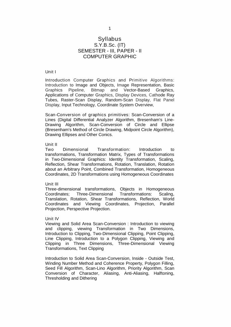
SyllabusS.Y.B.Sc. (IT)

SEMESTER - III, PAPER - IICOMPUTER GRAPHIC

Unit I

Introduction Computer Graphics and Primitive Algorithms:Introduction to Image and Objects, Image Representation, BasicGraphics Pipeline, Bitmap and Vector-Based Graphics,Applications of Computer Graphics, Display Devices, Cathode RayTubes, Raster-Scan Display, Random-Scan Display, Flat PanelDisplay, Input Technology, Coordinate System Overview,

Scan-Conversion of graphics primitives: Scan-Conversion of aLines (Digital Differential Analyzer Algorithm, Bresenham's Line-Drawing Algorithm, Scan-Conversion of Circle and Ellipse(Bresenham's Method of Circle Drawing, Midpoint Circle Algorithm),Drawing Ellipses and Other Conics.

Unit IITwo Dimensional Transformation: Introduction totransformations, Transformation Matrix, Types of Transformationsin Two-Dimensional Graphics: Identity Transformation, Scaling,Reflection, Shear Transformations, Rotation, Translation, Rotationabout an Arbitrary Point, Combined Transformation, HomogeneousCoordinates, 2D Transformations using Homogeneous Coordinates

Unit IIIThree-dimensional transformations, Objects in HomogeneousCoordinates; Three-Dimensional Transformations: Scaling,Translation, Rotation, Shear Transformations, Reflection, WorldCoordinates and Viewing Coordinates, Projection, ParallelProjection, Perspective Projection.

Unit IVViewing and Solid Area Scan-Conversion : Introduction to viewingand clipping, viewing Transformation in Two Dimensions,Introduction to Clipping, Two-Dimensional Clipping, Point Clipping,Line Clipping, Introduction to a Polygon Clipping, Viewing andClipping in Three Dimensions, Three-Dimensional ViewingTransformations, Text Clipping

Introduction to Solid Area Scan-Conversion, Inside - Outside Test,Winding Number Method and Coherence Property, Polygon Filling,Seed Fill Algorithm, Scan-Lino Algorithm, Priority Algorithm, ScanConversion of Character, Aliasing, Anti-Aliasing, Halftoning,Thresholding and Dithering

2

Unit VIntroduction to curves, Curve Continuity, Conic Curves, PiecewiseCurve Design, Parametric Curve Design, Spline CurveRepresentation, Bezier Curves, B-Spline Curves, Fractals and itsapplications.

Surface Design : Bilinear Surfaces, Ruled Surfaces, DevelopableSurfaces, Coons Patch, Sweep Surfaces, Surface of Revolution,Quadric Surfaces, Constructive Solid Geometry, Bezier Surfaces,B-Spline Surfaces, Subdivision Surfaces.

Visible Surfaces : Introduction to visible and hidden surfaces,Coherence for visibility, Extents and Bounding Volumes, Back FaceCulling, Painter’s Algorithm, Z-Buffer Algorithm, Floating HorizonAlgorithm, Roberts Algorithm.

Unit VIObject Rendering : Introduction Object-Rendering, Light ModelingTechniques, illumination Model, Shading, Flat Shading, PolygonMesh Shading, Gaurand Shading Model, Phong Shading,Transparency Effect, Shadows, Texture and ObjectRepresentation, Ray Tracing, Ray Casting, Radiosity, ColorModels.

Introduction to animation, Key-Frame Animation, Construction of anAnimation Sequence, Motion Control Methods, ProceduralAnimation, Key-Frame Animation vs. Procedural Animation,Introduction to Morphing, Three-Dimensional Morphing.

Books :Computer Graphics, R. K. Maurya, John Wiley.Mathematical elements of Computer Graphics, David F. Rogers, J.Alan Adams, Tata McGraw-Hill.Procedural elements of Computer Graphics, David F. Rogers, TataMcGraw-Hill.

Reference:Computer Graphics, Donald Hearn and M. Pauline Baker, PrenticeHall of India.Computer Graphics, Steven Harrington, McGraw-Hill.Computer Graphics Principles and Practice, J.D. Foley, A VanDam, S. K. Feiner and R. L. Phillips, Addision Wesley.Principles of Interactive Computer Graphics, William M. Newman,Robert F. Sproull, Tata McGraw-Hill.Introduction to Computer Graphics, J.D. Foley, A. Van Dam, S. K.Feiner, J.F. Hughes and R.L. Phillips, Addision Wesley.

3

Practical (Suggested) :Should contain at least 10 programs developed using C++. Somesample practical are listed below.1. Write a program with menu option to input the line coordinates

from the user to generate a line using Bresenham’s methodand DDA algorithm. Compare the lines for their values on theline.

2. Develop a program to generate a complete circle based on.

a) Bresenham’s circle algorithm

b) Midpoint Circle Algorithm

3. Implement the Bresenham’s / DDA algorithm for drawing line(programmer is expected to shift the origin to the center of thescreen and divide the screen into required quadrants)

4. Write a program to implement a stretch band effect. (A userwill click on the screen and drag the mouse / arrow keys overthe screen coordinates. The line should be updated likerubber-band and on the right-click gets fixed).

5. Write program to perform the following 2D and 3Dtransformations on the given input figure

a) Rotate through

b) Reflection

c) Scaling

d) Translation

6. Write a program to demonstrate shear transformation indifferent directions on a unit square situated at the origin.

7. Develop a program to clip a line using Cohen-Sutherland line

clipping algorithm between 1 1 2 2, ,X Y X Y against a window

min min max max, ,X Y X Y .

8. Write a program to implement polygon filling.

9. Write a program to generate a 2D/3D fractal figures (Sierpinskitriangle, Cantor set, tree etc).

10. Write a program to draw Bezier and B-Spline Curves withinteractive user inputs for control polygon defining the shapeof the curve.

11. Write a program to demonstrate 2D animation such as clocksimulation or rising sun.

12. Write a program to implement the bouncing ball inside adefined rectangular window.

4

1

COMPUTER GRAPHICS -FUNDAMENTALS

Unit Structure

1.0 Objectives

1.1 Introduction

1.2 Introduction to Image and Objects

1.3 Image Representation

1.4 Basic Graphics Pipeline

1.5 Bitmap and Vector-Based Graphics

1.6 Applications of Computer Graphics

1.7 Display Devices

1.7.1 Cathode Ray Tubes

1.7.2 Raster-Scan Display

1.7.3 Random-Scan Display

1.7.4 Flat Panel Display

1.8 Input Technology

1.9 Coordinate System Overview

1.10 Let us sum up

1.4 References and Suggested Reading

1.5 Exercise

1.0OBJECTIVES

The objective of this chapter is To understand the basics of computer graphics. To be aware of applications of computer graphics. To know the elements of computer graphics.

1.1 INTRODUCTION

Computer graphics involves display, manipulation andstorage of pictures and experimental data for proper visualizationusing a computer. It provides methods for producing images andanimations (sequence of images). It deals with the hardware aswell as software support for generating images.

5

Basically, there are four major operations that we perform incomputer graphics:

Imaging: refers to the representation of 2D images. Modeling: refers to the representation of 3D images. Rendering: refers to the generation of 2D images from 3D

models.

Animation: refers to the simulation of sequence of images overtime.

1.2 INTRODUCTION TO IMAGE AND OBJECTS

An image is basically representation of a real world object ona computer. Itcan be an actual picture display, a stored page in avideo memory, or a source code generated by a program.Mathematically, an image is a two - dimensional array of data withintensity or a color value at each element of the array.

Objects are real world entities defined in three – dimensionalworld coordinates. In computer graphics we deal with both 2D and3D descriptions of an object. We also study the algorithms andprocedures for generation and manipulation of objects and imagesin computer graphics.

Check your Progress:1. Define image and object.2. How an image is represented mathematically?

1.3 IMAGE REPRESENTATION

Image representation is the approximations of the real worlddisplayed in a computer. A picture in computer graphics isrepresented as a collection of discrete picture elements termed aspixels. A pixel is the smallest element of picture or object that canbe represented on the screen of a device like computer.

6

Check your progress:1. Define pixel.

1.4 BASIC GRAPHIC PIPELINE

In computer graphics, the graphics pipeline refers to a seriesof interconnected stages through which data and commandsrelated to a scene go through during rendering process.

It takes us from the mathematical description of an object toits representation on the device.

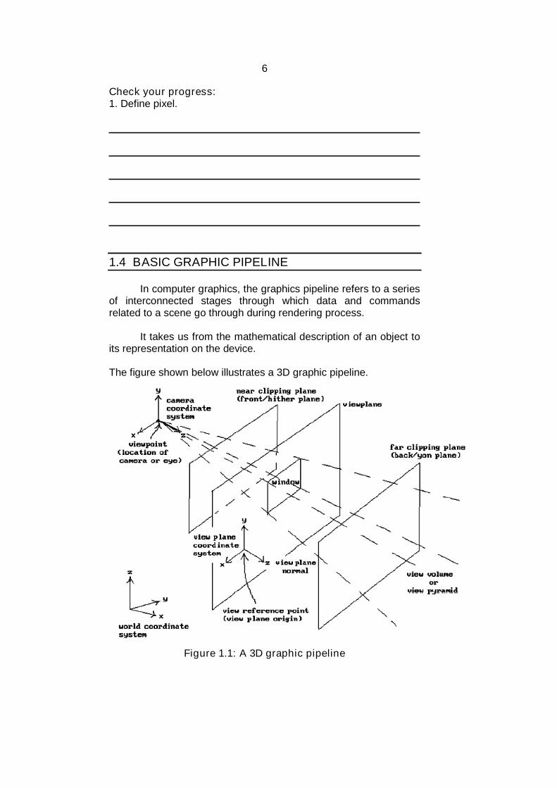
The figure shown below illustrates a 3D graphic pipeline.

Figure 1.1: A 3D graphic pipeline

7

The real world objects are represented in world coordinatesystem. It is then projected onto a view plane. The projection isdone from the viewpoint of the position of a camera or eye. There isan associated camera coordinate system whose z axis specifiesthe view direction when viewed from the viewpoint. The infinitevolume swept by the rays emerging from the viewpoint and passingthrough the window is called as view volume or view pyramid.Clipping planes (near and far) are used to limit the output of theobject.

The mapping of an object to a graphic device requires thetransformation of view plane coordinates to physical devicecoordinates. There are two steps involved in this process.

(i) The window to a viewport transformation. The viewport isbasically a sub – rectangle of a fixed rectangle known aslogical screen.

(ii) The transformation of logical screen coordinates to physicaldevice coordinates.

Figure : Sequence of transformation in viewing pipeline

Figure 1.2: 2D coordinate system to physical devicecoordinates transformation.

The figures above depict the graphic pipeline and the 2Dcoordinate transformation to physical device coordinates.

Representationof 3D world

objects

Clip againstview volume

Transform tophysical devicecoordinates

Transform toviewport

Project to viewplane

Transform intocamera

coordinates

Clip againstwindow

Transform tophysical device

coordinates

Transport toviewport

Representationof 2D world

objects

8

Check your Progress:1. Differentiate between world coordinates system and camera

coordinate system.2. Define view volume.

1.5 BITMAP AND VECTOR – BASED GRAPHICS

Computer graphics can be classified into two categories:Raster or Bitmap graphics and Vector graphics.

Bitmap graphics: It is pixel based graphics. The position and color information about the image are

stored in pixels arranged in grid pattern. The Image size is determined on the basis of image

resolution. These images cannot be scaled easily. Bitmap images are used to represent photorealistic images

which involve complex color variations.

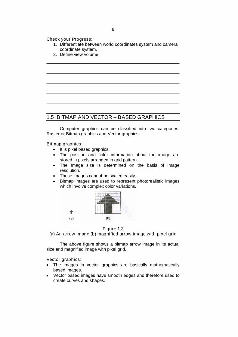
Figure 1.3(a) An arrow image (b) magnified arrow image with pixel grid

The above figure shows a bitmap arrow image in its actualsize and magnified image with pixel grid.

Vector graphics: The images in vector graphics are basically mathematically

based images. Vector based images have smooth edges and therefore used to

create curves and shapes.

9

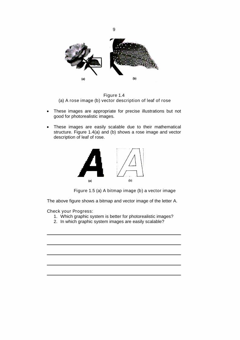
Figure 1.4(a) A rose image (b) vector description of leaf of rose

These images are appropriate for precise illustrations but notgood for photorealistic images.

These images are easily scalable due to their mathematicalstructure. Figure 1.4(a) and (b) shows a rose image and vectordescription of leaf of rose.

Figure 1.5 (a) A bitmap image (b) a vector image

The above figure shows a bitmap and vector image of the letter A.

Check your Progress:1. Which graphic system is better for photorealistic images?2. In which graphic system images are easily scalable?

10

1.6 APPLICATIONS OF COMPUTER GRAPHICS

Computer graphics finds its application in various areas; some ofthe important areas are discussed below:

Computer-Aided Design: In engineering and architecturalsystems, the products are modeled using computer graphicscommonly referred as CAD (Computer Aided Design).

In many design applications like automobiles, aircraft,spacecraft, etc., objects are modeled in a wireframe outline thathelps the designer to observe the overall shape and internalfeatures of the objects.

CAD applications are also used in computer animations. Themotion of an object can be simulated using CAD.

Presentation graphics: In applications like summarizing ofdata of financial, statistical, mathematical, scientific andeconomic research reports, presentation graphics are used. Itincreases the understanding using visual tools like bar charts,line graphs, pie charts and other displays.

Computer Art: A variety of computer methods are available forartists for designing and specifying motions of an object. Theobject can be painted electronically on a graphic tablet usingstylus with different brush strokes, brush widths and colors. Theartists can also use combination of 3D modeling packages,texture mapping, drawing programs and CAD software to paintand visualize any object.

Entertainment: In making motion pictures, music videos andtelevision shows, computer graphics methods are widely used.Graphics objects can be combined with live actions or can beused with image processing techniques to transform one objectto another (morphing).

Education and training: Computer graphics can make usunderstand the functioning of a system in a better way. Inphysical systems, biological systems, population trends, etc.,models makes it easier to understand.

In some training systems, graphical models with simulationshelp a trainee to train in virtual reality environment. Forexample, practice session or training of ship captains, aircraftpilots, air traffic control personnel.

11

Visualization: For analyzing scientific, engineering, medicaland business data or behavior where we have to deal with largeamount of information, it is very tedious and ineffective processto determine trends and relationships among them. But if it isconverted into visual form, it becomes easier to understand.This process is termed as visualization.

Image processing: Image processing provides us techniquesto modify or interpret existing images. One can improve picturequality through image processing techniques and can also beused for machine perception of visual information in robotics.

In medical applications, image processing techniques can beapplied for image enhancements and is been widely used forCT (Computer X-ray Tomography) and PET (Position EmissionTomography) images.

Graphical User Interface: GUI commonly used these days tomake a software package more interactive. There are multiplewindow system, icons, menus, which allows a computer setupto be utilized more efficiently.

Check your progress:

1. Fill in the blanks

(a) GUI stands for.................

(b) ............ provides us techniques to modify or interpret existingimages.

2. Explain how computer graphics are useful in entertainmentindustry.

1.7 DISPLAY DEVICES

There are various types of displays like CRT, LCD andPlasma. We will discuss each of these three in brief.

12

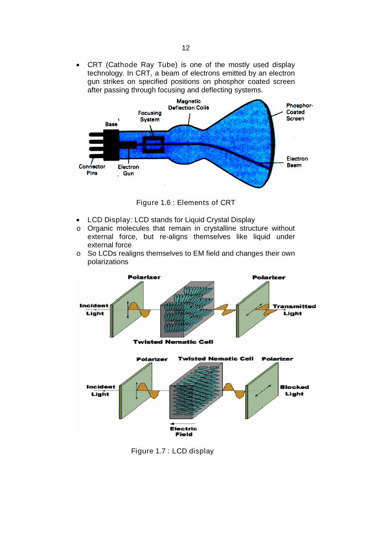
CRT (Cathode Ray Tube) is one of the mostly used displaytechnology. In CRT, a beam of electrons emitted by an electrongun strikes on specified positions on phosphor coated screenafter passing through focusing and deflecting systems.

Figure 1.6 : Elements of CRT

LCD Display: LCD stands for Liquid Crystal Displayo Organic molecules that remain in crystalline structure without

external force, but re-aligns themselves like liquid underexternal force

o So LCDs realigns themselves to EM field and changes their ownpolarizations

Figure 1.7 : LCD display

13

o There are two types of LCD displays:

o Active Matrix LCD: Electric field is retained by a capacitor so that the crystal

remains in a constant state. Transistor switches are used to transfer charge into the

capacitors during scanning. The capacitors can hold the charge for significantly longer than

the refresh period Crisp display with no shadows. More expensive to produce.

o Passive matrix LCD: LCD slowly transit between states. In scanned displays, with a large number of pixels, the

percentage of the time that LCDs are excited is very small. Crystals spend most of their time in intermediate states, being

neither "On" or "Off". These displays are not very sharp and are prone to ghosting.

Plasma display:

Figure1.8 (showing the basic structure of plasma display)

o These are basically fluorescent tubes.o High- voltage discharge excites gas mixture (He, Xe), upon

relaxation UV light is emitted, UV light excites phosphors.o Some of its features are Large view angle Large format display Less efficient than CRT, more power Large pixels: 1mm (0.2 mm for CRT) Phosphors depletion

In CRT monitors there are two techniques of displaying images.

14

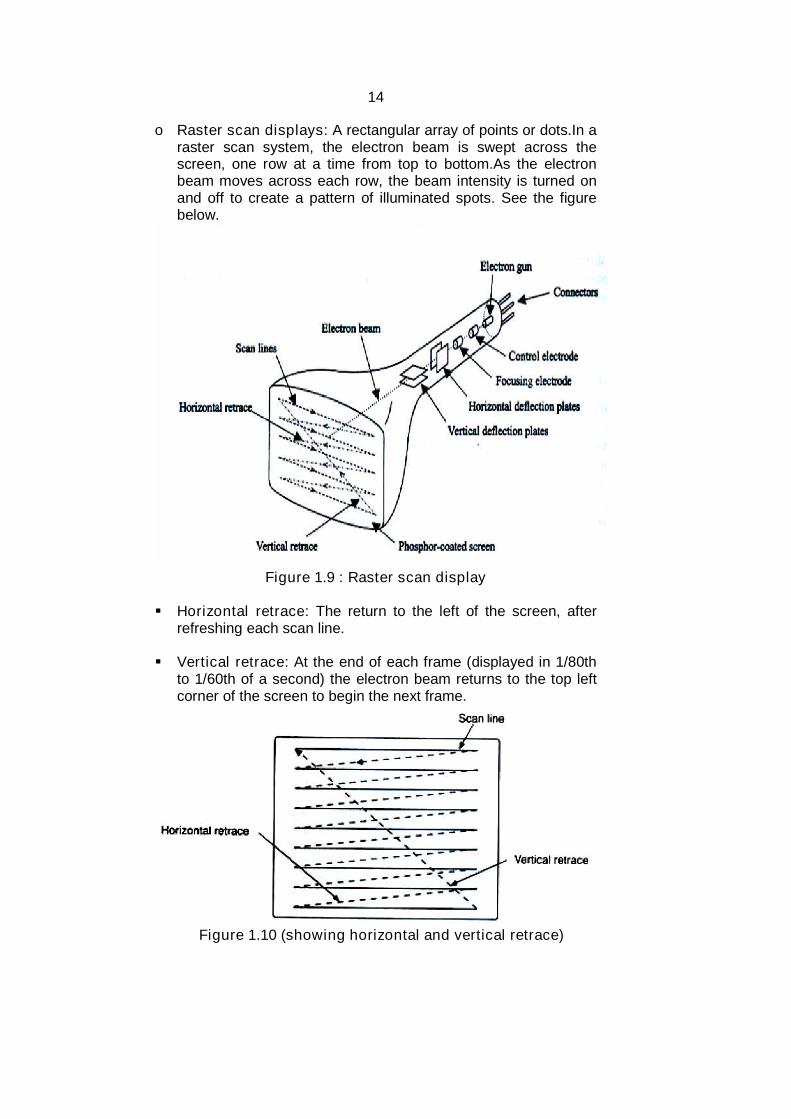
o Raster scan displays: A rectangular array of points or dots.In araster scan system, the electron beam is swept across thescreen, one row at a time from top to bottom.As the electronbeam moves across each row, the beam intensity is turned onand off to create a pattern of illuminated spots. See the figurebelow.

Figure 1.9 : Raster scan display

Horizontal retrace: The return to the left of the screen, afterrefreshing each scan line.

Vertical retrace: At the end of each frame (displayed in 1/80thto 1/60th of a second) the electron beam returns to the top leftcorner of the screen to begin the next frame.

Figure 1.10 (showing horizontal and vertical retrace)

15

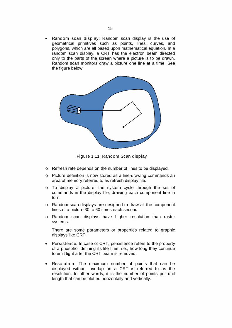
Random scan display: Random scan display is the use ofgeometrical primitives such as points, lines, curves, andpolygons, which are all based upon mathematical equation. In arandom scan display, a CRT has the electron beam directedonly to the parts of the screen where a picture is to be drawn.Random scan monitors draw a picture one line at a time. Seethe figure below.

Figure 1.11: Random Scan display

o Refresh rate depends on the number of lines to be displayed.

o Picture definition is now stored as a line-drawing commands anarea of memory referred to as refresh display file.

o To display a picture, the system cycle through the set ofcommands in the display file, drawing each component line inturn.

o Random scan displays are designed to draw all the componentlines of a picture 30 to 60 times each second.

o Random scan displays have higher resolution than rastersystems.

There are some parameters or properties related to graphicdisplays like CRT:

Persistence: In case of CRT, persistence refers to the propertyof a phosphor defining its life time, i.e., how long they continueto emit light after the CRT beam is removed.

Resolution: The maximum number of points that can bedisplayed without overlap on a CRT is referred to as theresolution. In other words, it is the number of points per unitlength that can be plotted horizontally and vertically.

16

Aspect ratio: It is the ratio of the number of vertical points tothe number of horizontal points necessary to produce equal-length lines in both directions on the screen.

Frame buffer: Frame buffer also known as refresh buffer is thememory area that holds the set of intensity values for all thescreen points.

Pixel: It refers a point on the screen. It is also known as pel andis shortened form of ‘picture element’.

Bitmap or pixmap: A frame buffer is said to be bitmap on ablack and white system with one bit per pixel. For systems withmultiple bits per pixel, the frame buffer is referred to as pixmap.

Graphical images - used to add emphasis, direct attention,illustrate concepts, and provide background content. Two typesof graphics:

o Draw-type graphics or vector graphics – represent an image asa geometric shape

o Bitmap graphics – represents the image as an array of dots,called pixels

Three basic elements for drawing in graphics are:

o Point: A point marks a position in space. In pure geometricterms, a point is a pair of x, y coordinates. It has no mass at all.Graphically, however, a point takes form as a dot, a visiblemark. A point can be an insignificant fleck of matter or aconcentrated locus of power. It can penetrate like a bullet,pierce like a nail, or pucker like a kiss. A mass of pointsbecomes texture, shape, or plane. Tiny points of varying sizecreate shades of gray.

o Line: A line is an infinite series of points. Understoodgeometrically, a line has length, but no breadth. A line is theconnection between two points, or it is the path of a movingpoint. A line can be a positive mark or a negative gap. Linesappear at the edges of objects and where two planes meet.Graphically, lines exist in many weights; the thickness andtexture as well as the path of the mark determine its visualpresence. Lines are drawn with a pen, pencil, brush, mouse, ordigital code. They can be straight or curved, continuous orbroken. When a line reaches a certain thickness, it becomes aplane. Lines multiply to describe volumes, planes, and textures.

o Plane: A plane is a flat surface extending in height and width. Aplane is the path of a moving line; it is a line with breadth. A linecloses to become a shape, a bounded plane. Shapes are

17

planes with edges. In vector–based software, every shapeconsists of line and fill. A plane can be parallel to the picturesurface, or it can skew and recede into space. Ceilings, walls,floors, and windows are physical planes. A plane can be solid orperforated, opaque or transparent, textured or smooth.

Check your progress:1. Explain different display technologies.2. Differentiate between Raster scan and Random scan display.

1.8 INPUT TECHNOLOGY

There are different techniques for information input ingraphical system. The input can be in the form of text, graphic orsound. Some of the commonly used input technologies arediscussed below.

1.8.1Touch ScreensA touch screen device allows a user to operate a touch

sensitive device by simply touching the display screen. The inputcan be given by a finger or passive objects like stylus. There arethree components of a touch screen device: a touch sensor, acontroller and a software driver.

A touch sensor is a touch sensitive clear glass panel. Acontroller is a small PC card which establishes the connectionbetween a touch sensor and the PC. The software driver is asoftware that allows the touch screen to work together with the PC.The touch screen technology can be implemented in various wayslike resistive, surface acoustic, capacitive, infrared, strain gauge,optical imaging, dispersive signal technology, acoustic pulserecognition and frustrated total internal reflection.

1.8.2Light penA light pen is pen shaped pointing device which is connected

to a visual display unit. It has light sensitive tip which detects thelight from the screen when placed against it which enables acomputer to locate the position of the pen on the screen. Users can

18

point to the image displayed on the screen and also can draw anyobject on the screen similar to touch screen with more accuracy.

1.8.3 Graphic tabletsGraphic tablets allow a user to draw hand draw images and

graphics in the similar way as is drawn with a pencil and paper.

It consists of a flat surface upon which the user can draw ortrace an image with the help of a provided stylus. The image isgenerally displayed on the computer monitor instead of appearingon the tablet itself.

Check your Progress:1. Name different types of touch screen technologies.2. Differentiate between light pen and graphic tablet.

1.9 COORDINATE SYSTEM OVERVIEW

To define positions of points in space one requires acoordinate system. It is way of determining the position of a pointby defining a set of numbers called as coordinates. There aredifferent coordinate systems for representing an object in 2D or 3D.

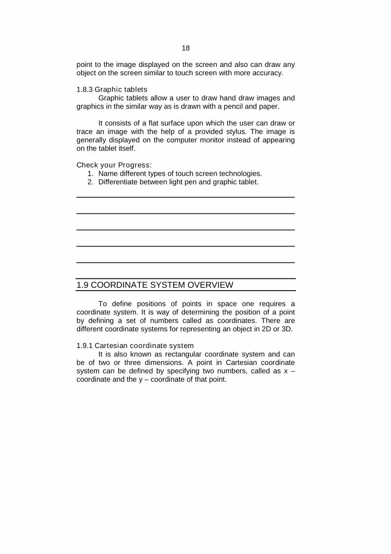
1.9.1 Cartesian coordinate systemIt is also known as rectangular coordinate system and can

be of two or three dimensions. A point in Cartesian coordinatesystem can be defined by specifying two numbers, called as x –coordinate and the y – coordinate of that point.

19

.

Figure 1.12: Cartesian coordinate system

In the above figure, there are two points (2, 3) and (3, 2) arespecified in Cartesian coordinate system

1.9.2 Polar coordinate systemIn polar coordinate system, the position of a point is defined byspecifying the distance (radius) from a fixed point called as originand the angle between the line joining the point and the origin andthe polar axis (horizontal line passing through the origin).

Figure 1.13: Polar coordinate system

The above figure shows a point (r, θ) in polar coordinates.

20

Check your Progress:

Fill in the blanks1. The position of a point is defined by specifying the distance

(radius) from a fixed point called as ……….

2. A point in Cartesian coordinate system can be defined byspecifying two numbers, called as …….. and the ………… ofthat point.

Answers: 1. Origin2. x - coordinate, y – coordinate.

1.10 LET US SUM UP

We learnt about computer graphics, its application indifferent areas. We studied various display and input technologies.We also studied basic graphic pipeline, bitmap and vector basedgraphics. Then we learnt the elements of computer graphics inwhich came to know about the terms like persistence, resolution,aspect ratio, frame buffer, pixel and bitmap. Finally we studiedabout the coordinate system.

1.11 REFERENCES AND SUGGESTED READING

(1) Computer Graphics, Donald Hearn, M P. Baker, PHI.

(2) Procedural elements of Computer Graphics, David F. Rogers,Tata McGraw Hill.

(3) Computer Graphics, Rajesh K. Maurya, Wiley - India

1.12 EXERCISE

1. What are the major operations that we perform on ComputerGraphics?

2. Define some of the applications of Computer Graphics.

21

3. Define graphic pipeline and the process involved in it.

4. Differentiate between bitmap and vector based graphics.

5. Define the following terms:a. Persistenceb. Aspect ratioc. Frame bufferd. Resolutione. Pixel

6. Define horizontal and vertical retrace.

22

2

SCAN CONVERSION OF GRAPHICSPRIMITIVES

Unit Structure

2.0 Objectives

2.1 Introduction

2.2Scan-Conversion of a Lines

2.3Scan- Conversion of Circle and Ellipse

2.3.1 Digital Differential Analyzer Algorithm

2.3.2 Bresenham's Line-Drawing Algorithm

2.4Drawing Ellipses and Other Conics

2.4.1 Bresenham's Method of Circle Drawing

2.4.2 Midpoint Circle Algorithm

2.5Drawing Ellipses and Other Conics

2.6Let us sum up

2.7References and Suggested Reading

2.8Exercise

2.0 OBJECTIVES

The objective of this chapter is To understand the basic idea of scan conversion techniques. To understand the algorithms for scan conversion of line,

circle and other conics.

2.1 INTRODUCTION

Scan conversion or rasterization is the process of convertingthe primitives from its geometric definition into a set of pixels thatmake the primitive in image space. This technique is used to drawshapes like line, circle, ellipse, etc. on the screen. Some of themare discussed below

23

2.2 SCAN – CONVERSION OF LINES

A straight line can be represented by a slope intercept equationas

where m represents the slope of the line and b as the yintercept.

If two endpoints of the line are specified at positions (x1,y1) and(x2,y2), the values of the slope m and intercept b can bedetermined as

If ∆x and ∆y are the intervals corresponding to x and y respectively for a line, then for given interval ∆x, we can calculate ∆y.

Similarly for given interval ∆y, ∆x can be calculated as

For lines with magnitude |m| < 1, ∆x can be set proportional to a small horizontal deflection and the corresponding horizontaldeflection is et proportional to ∆y and can be calculated as

For lines with |m|>1, ∆y can be set proportional to small vertical deflection and corresponding ∆x which is set proportional to

horizontal deflection is calculated using

The following shows line drawn between points (x1, y1) and (x2, y2).

Figure 2.1 : A line representation in Cartesian coordinatesystem

24

2.2.1 Digital Differential Analyzer (DDA) Algorithm

Sampling of the line at unit interval is carried out in onecoordinate and corresponding integer value for the othercoordinate is calculated.

If the slope is less than or equal to 1( |m| ≤ 1), the coordinate xis sampled at unit intervals (∆x = 1) and each successive values of y is computed as

where k varies from 1 to the end point value taking integervalues only. The value of y calculated is rounded off to thenearest integer value.

For slope greater than 1 (|m| > 1), the roles of y and x arereversed, i.e., y is sampled at unit intervals (∆y = 1) and corresponding x values are calculated as

For negative value slopes, we follow the same procedure asabove, only the sampling unit ∆x and ∆y becomes ‘-1’ and

Pseudocode for DDA algorithm is as followsLineDDA(Xa, Ya, Xb, Yb) // to draw a line from (Xa, Ya) to(Xb, Yb)

{Set dx = Xb - Xa, dy = Yb - Ya;Set steps = dx;SetX = Xa, Y = Ya;int c = 0;Call PutPixel(Xa, ya);For (i=0; i <steps; i++)

{X = X + 1;

c = c + dy; // update the fractional partIf (c > dx)

{ // (that is, the fractional part is greater than 1now

Y = y +1; // carry the overflowed integer overc = c - dx // update the fractional part

Call PutPixel(X, Y);}}

}

25

2.2.2 Bresenham’s Line Drawing Algorithm

This line drawing algorithm proposed by Bresenham, is anaccurate and efficient raster-line generating algorithm using onlyincremental integer calculations.

For lines |m| ≤ 1, the Bresenham’s line drawing algorithm

I. Read the end points of the line and store left point in (x0, y0)

II. Plot (x0, y0), the first point.

III. Calculate constants ∆x, ∆y, 2∆y and 2∆y - 2∆x, and obtain a decision parameter p0

IV. Perform the following test for each xk, starting at k = 0 if pk<0, then next plotting point is (xk+1, yk) and

Otherwise, the next point to plot is (xk+1, yk+1) and

V. Repeat step 4 ∆x times.For a line with positive slope more than 1, the roles of the x

and y directions are interchanged.


1. Fill in the blanks

(a) ............of the line at unit interval is carried out in one coordinateand corresponding integer value for the other coordinate iscalculated.

(b) Bresenham's line drawing algorithm is an accurate and efficientraster-line generating algorithm using only ................calculations.

2. Compare DDA and Bresenham's line drawing algorithm.

Answers: 1(a) sampling (b) incremental integer

.

26

2.3 SCAN – CONVERSION OF CIRCLE AND ELLIPSE

A circle with centre (xc, yc) and radius r can be represented inequation form in three ways

Analytical representation: r2 = (x – xc)2 + (y – yc)

2

Implicit representation : (x – xc)2 + (y – yc)

2 – r2 = 0 Parametric representation: x = xc + r cosθ

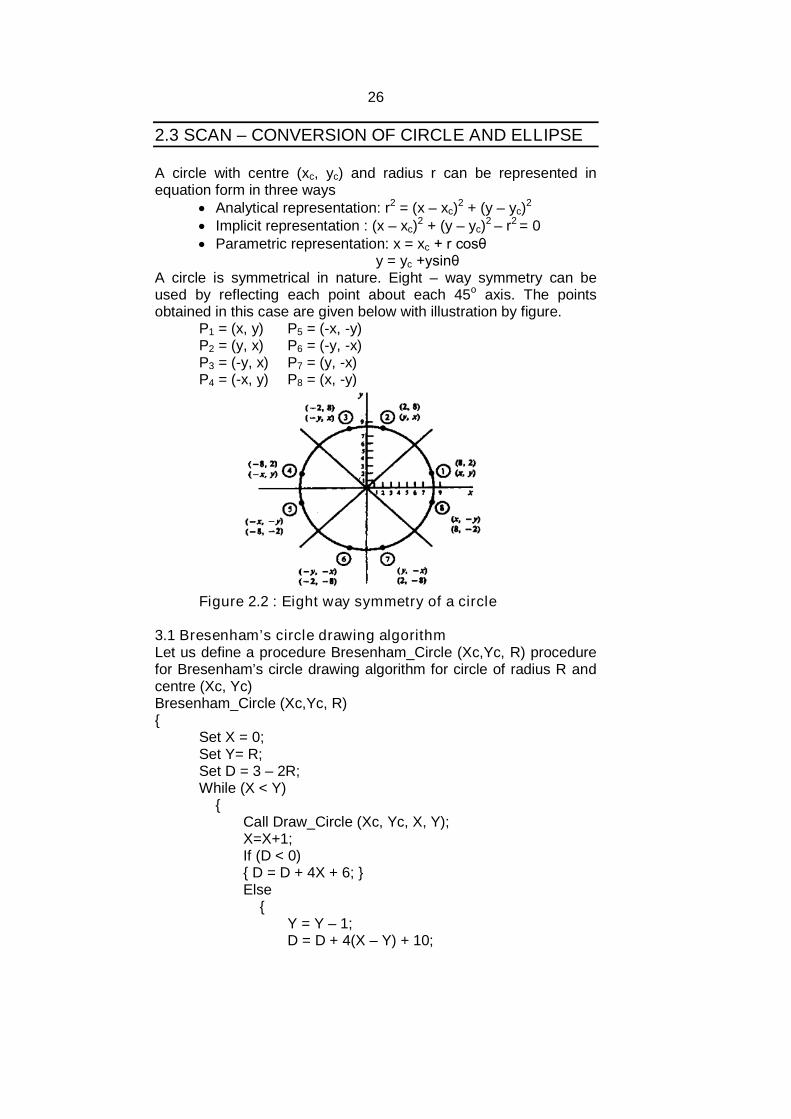
y = yc +ysinθA circle is symmetrical in nature. Eight – way symmetry can beused by reflecting each point about each 45o axis. The pointsobtained in this case are given below with illustration by figure.

P1 = (x, y) P5 = (-x, -y)P2 = (y, x) P6 = (-y, -x)P3 = (-y, x) P7 = (y, -x)P4 = (-x, y) P8 = (x, -y)

Figure 2.2 : Eight way symmetry of a circle

3.1 Bresenham’s circle drawing algorithmLet us define a procedure Bresenham_Circle (Xc,Yc, R) procedurefor Bresenham’s circle drawing algorithm for circle of radius R andcentre (Xc, Yc)Bresenham_Circle (Xc,Yc, R){

Set X = 0;Set Y= R;Set D = 3 – 2R;While (X < Y)

{Call Draw_Circle (Xc, Yc, X, Y);X=X+1;If (D < 0){ D = D + 4X + 6; }Else

{Y = Y – 1;D = D + 4(X – Y) + 10;

27

}Call Draw_Circle (Xc, Yc, X, Y);}

}Draw_Circle (Xc, Yc, X, Y)

{Call PutPixel (Xc + X, Yc, +Y);Call PutPixel (Xc – X, Yc, +Y);Call PutPixel (Xc + X, Yc, – Y);Call PutPixel (Xc – X, Yc, – Y);Call PutPixel (Xc + Y, Yc, + X);Call PutPixel (Xc – Y ,Yc, – X);Call PutPixel (Xc + Y, Yc, – X);Call PutPixel (Xc – Y, Yc, – X);

}

2.3.2Midpoint circle drawing algorithmThis algorithm uses the implicit function of the circle in the followingwayf (x, y) = (x – xc)

2 + (y – yc)2 – r2

here f (x, y) < 0 means (x, y) is inside the circlef ( x, y) = 0 means (x, y) is on the circlef (x, y) > 0 means (x, y) is outside the circleThe algorithm now follows as

Midpoint_Circle( Xc, Yc, R){

Set X = 0;Set Y = R;Set P = 1 – R;While (X < Y)

{Call Draw_Circle( Xc, Yc, X, Y);X = X + 1;If (P < 0){P = P + 2X + 6; }Else

{Y = Y – 1;P = P + 2 (X – Y) + 1;

}Call Draw_Circle( Xc, Yc, X, Y);

}}

2.3.3 Midpoint Ellipse AlgorithmThis is a modified form of midpoint circle algorithm for drawingellipse. The general equation of an ellipse in implicit form isf (x, y) = b2x2 + a2y2 – a2b2 = 0

28

Now the algorithm for ellipse follows asMidPoint_Ellipse( Xc, Yc, Rx, Ry)

{/* Xc and Yc here denotes the x coordinate and ycoordinate of the center of the ellipse and Rx and Ryare the x-radius and y-radius of the ellipserespectively */Set Sx = Rx * Rx;Set Sy = Ry * Ry;Set X = 0;Set Y = Ry;Set Px = 0;Set Py = 2 * Sx * Y;Call Draw_Ellipse (Xc, Yc, X, Y);Set P = Sy – (Sx * Ry) + (0.25 * Sx);/* First Region*/While ( Px<Py)

{X = X + 1;Px = Px + 2 * Sy;If (P < 0)

{P = P + Sy + Px;}Else

{Y = Y – 1;Py = Py – 2 * Sx;P = P + Sy + Px – Py;

}Call Draw_Ellipse (Xc, Yc, X, Y);

}P = Sy * (X + 0.5)2 + Sx * (Y – 1)2 – Sx * Sy;

/*Second Region*/While (Y > 0)

{Y = Y – 1;Py = Py – 2 * Sx;If (P > 0)

{P = P + Sx – Py;}Else

{X = X + 1;Px = Px + 2 * Sy;P = P + Sx – Py + Px;

}Call Draw_Ellipse (Xc, Yc, X, Y);

}}

Draw_Ellipse (Xc, Yc, X, Y){

29

Call PutPixel (Xc + X, Yc + Y);Call PutPixel (Xc – X, Yc + Y);Call PutPixel (Xc + X, Yc – Y);Call PutPixel (Xc – X, Yc – Y);

}

Check your progress:1. Give three representations of circle, also give their equations.2. Fill in the blanks

In midpoint circle drawing algorithm iff (x, y) < 0 means (x, y) is ......the circlef ( x, y) = 0 means (x, y) is ......the circlef (x, y) > 0 means (x, y) is ........the circleAnswers: 2. inside, on, outside

2.4 DRAWING ELLIPSES AND OTHER CONICS

The equation of an ellipse with center at the origin is given as

Using standard parameterization, we can generate points on it as

Differentiating the standard ellipse equation we get

Now the DDA algorithm for circle can be applied to draw the ellipse.Similarly a conic can be defined by the equation

If starting pixel on the conic is given, the adjacent pixel can bedetermined similar to the circle drawing algorithm.

30

Check your Progress:1. Write down the equation of a standard ellipse.2. Which scan conversion technique can be applied to draw an

ellipse?

2.5 LET US SUM UP

We learnt about the scan conversion technique and how it isused to represent line, circle and ellipse. The DDA andBresenham’s line drawing algorithm were discussed. We thenlearnt Bresenham’s and Midpoint circle drawing algorithm. Midpointellipse drawing algorithm was also illustrated. Finally we learntabout drawing ellipse and other conics.


(1) Computer Graphics, Donald Hearn, M P. Baker, PHI.(4) Procedural elements of Computer Graphics, David F. Rogers,

Tata McGraw Hill.(5) Computer Graphics, Rajesh K. Maurya, Wiley – India.

2.7 EXERCISE

7. Describe scan conversion?8. Explain briefly the DDA line drawing algorithm.9. Explain the Bresenham’s line drawing algorithm with

example.10. Discuss scan conversion of circle with Bresenham’s and

midpoint circle algorithms.11.Explain how ellipse and other conics can be drawn using

scan conversion technique.

31

3

TWO DIMENSIONALTRANSFORMATIONS I

Unit Structure

3.0 Objectives

3.1 Introduction

3.2 Introduction to transformations

3.3 Transformation Matrix

3.4 Types of Transformations in Two-Dimensional Graphics

3.5 Identity Transformation

3.6 Scaling

3.7 Reflection

3.8 Shear Transformations

3.9 Let us sum up


3.11 Exercise

3.0 OBJECTIVES

The objective of this chapter is To understand the basics of 2D transformations. To understand transformation matrix and types of 2D

transformations. To understand two dimensional Identity transformations. To understand 2D Scaling and Reflection transformations. To understand Shear transformations in 2D.

3.1 INTRODUCTION

Transformations are one of the fundamental operationsthat are performed in computer graphics. It is often required whenobject is defined in one coordinate system and is needed toobserve in some other coordinate system. Transformations are alsouseful in animation. In the coming sections we will see differenttypes of transformation and their mathematical form.

32

3.2 INTRODUCTION TO TRANSFORMATIONS

In computer graphics we often require to transform the coordinatesof an object (position, orientation and size). One can view objecttransformation in two complementary ways:

(i) Geometric transformation: Object transformation takes placein relatively stationary coordinate system or background.

(ii) Coordinate transformation: In this view point, coordinatesystem is transformed instead of object.

On the basis of preservation, there are three classes oftransformation

Rigid body: Preserves distance and angle. Example –translation and rotation

Conformal: Preserves angles. Example- translation, rotationand uniform scaling

Affine: Preserves parallelism, means lines remains lines.Example- translation, rotation, scaling, shear and reflection

In general there are four attributes of an object that may betransformed

(i) Position(translation)(ii) Size(scaling)(iii) Orientation(rotation)(iv)Shapes(shear)

Check your progress:1. Differentiate between geometrical and coordinate transformation.2. Fill in the blanks

(a) Rigid body transformation preserves...........(b) Conformal transformation preserves............(c) Affine transformation preserves...............

Answers: 2(a) distance and angle (b) angles (c) parallelism

3.3 TRANSFORMATION MATRIX

Transformation matrix is a basic tool for transformation.A matrix with n m dimensions is multiplied with the coordinate of

objects. Usually 3 3 or 4 4 matrices are used for transformation.

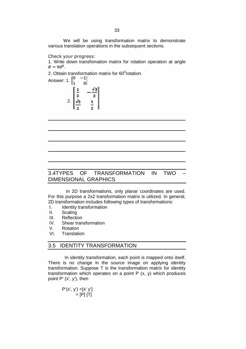
For example consider the following matrix for rotation operation

33

We will be using transformation matrix to demonstratevarious translation operations in the subsequent sections.

Check your progress:1. Write down transfomation matrix for rotation operation at angle

.

2. Obtain transformation matrix for 600rotation.

Answer: 1.

2.

3.4TYPES OF TRANSFORMATION IN TWO –DIMENSIONAL GRAPHICS

In 2D transformations, only planar coordinates are used.For this purpose a 2x2 transformation matrix is utilized. In general,2D transformation includes following types of transformations:I. Identity transformationII. ScalingIII. ReflectionIV. Shear transformationV. RotationVI. Translation

3.5 IDENTITY TRANSFORMATION

In identity transformation, each point is mapped onto itself.There is no change in the source image on applying identitytransformation. Suppose T is the transformation matrix for identitytransformation which operates on a point P (x, y) which producespoint P’ (x’, y’), then

P’(x’, y’) =[x’ y’]= [P] [T]

34

= [x y]

=[x y]We can see that on applying identity transformation we

obtain the same points. Here the identity transformation is

[T] =

The identity transformation matrix is basically anxn matrixwith ones on the main diagonal and zeros for other values.

Check your progress:Fill in the blanks

1. In identity transformation, each point is mapped onto …….2. The identity transformation matrix is basically anxn matrix

with …… on the main diagonal and ……. for other values.

Answers: 1. Itself2. ones, zeros.

3.6 SCALING

This transforms changes the size of the object. Weperform this operation by multiplying scaling factors sx and sy to theoriginal coordinate values (x, y) to obtain scaled new coordinates(x’, y’).

x'= x. sx y'= y. sy

In matrix form it can be represented as

For same sx and sy, the scaling is called as uniform scaling.For different sx and sy , the scaling is called as differential scaling.

Check your Progress:Fill in the blanks

1. Scaling changes the ……… of the object.2. For same sx and sy, the scaling is called as ………. Scaling.

Answers: 1. Size.2. uniform.

3.7REFLECTION

In reflection transformation, the mirror image of an objectis formed. In two dimensions, it is achieved through rotating theobject by 180 degrees about an axis known as axis of reflectionlying in a plane. We can choose any plane of reflection in xy planeor perpendicular to xy plane.

35

For example, reflection about x axis (y = 0) plane can bedone with the transformation matrix

Figure 3.1 : Reflection transformation about x axis

A reflection about y axis (x = 0) is shown in the figure belowwhich can be done by following transformation matrix.

Figure 3.2 : Reflection about y axis

Check Your Progress:Fill in the blanks1. In reflection transformation,

the ……… image of an object is formed.2. 2D reflection transformation

can be achieved through rotating the object by …….degrees.

Answers: 1. Mirror2. 180.

36

3.8 SHEAR TRANSFORMATIONS

An object can be considered to be composed of differentlayers. In shear transformation, the shape of the object is distortedby producing the sliding effect of layers over each other. There aretwo general shearing transformations, one which shift coordinatesof x axis and the other that shifts y coordinate values.

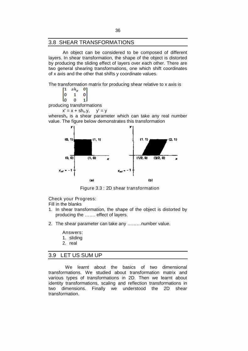
The transformation matrix for producing shear relative to x axis is

producing transformationsx' = x + shx.y, y' = y

whereshx is a shear parameter which can take any real numbervalue. The figure below demonstrates this transformation

Figure 3.3 : 2D shear transformation

Check your Progress:Fill in the blanks1. In shear transformation, the shape of the object is distorted by

producing the ……. effect of layers.

2. The shear parameter can take any ………number value.

Answers:1. sliding2. real

3.9 LET US SUM UP

We learnt about the basics of two dimensionaltransformations. We studied about transformation matrix andvarious types of transformations in 2D. Then we learnt aboutidentity transformations, scaling and reflection transformations intwo dimensions. Finally we understood the 2D sheartransformation.

37




3.11 EXERCISE

1. Explain transformation and its importance.2. Describe using transformation matrix, following 2D

transformations(i) Translation (ii) Scaling (iii) Reflection

3. Scale a triangle with respect to the origin, with vertices at originalcoordinates (10,20), (10,10), (20,10) by sx=2, sy=1.5.

4. What is the importance of homogenous coordinates?

5. Explain two dimensional shear transformations.

6. Obtain the transformation matrix for reflection along diagonal line(y = x axis).

Answers: 3. (20,30), (20,15), and (40,15)

38

4

TWO DIMENSIONALTRANSFORMATIONS II

Unit Structure

4.0 Objectives

4.1 Introduction

4.2 Rotation

4.3 Translation

4.4 Rotation about an Arbitrary Point

4.5 Combined Transformation

4.6 Homogeneous Coordinates

4.7 2D Transformations using Homogeneous Coordinates

4.8 Let us sum up


4.10 Exercise

4.0 OBJECTIVES

The objective of this chapter is To understand 2D rotation transformation. To understand 2D translation transformations. To understand two dimensional combined transformations. To understand homogenous coordinates and 2D

transformation using homogenous coordinates. To understand Shear transformations in 2D.

4.1 INTRODUCTION

This chapter is the extension of the previous chapter inwhich we will discuss the rotation transformation about origin andabout any arbitrary point. We will also learn about the translationtransformation in which the position of an object changes. Thehomogenous coordinates and 2D transformation usinghomogenous coordinates will also be explained.

39

4.2 ROTATION

In rotation transformation, an object is repositionedalong a circular path in the xy plane. The rotation is performed withcertain angle θ, known as rotation angle. Rotation can be performed in two ways: about origin or about an arbitrary pointcalled as rotation point or pivot point.

Rotation about origin: The pivot point here is the origin. We canobtain transformation equations for rotating a point (x, y) through anangleθ to obtain final point as (x’, y’) with the help of figure as

x' = x cosθ – y sinθy' = x sinθ + y cosθ

(x, y)r

r

(x , y )¢ ¢

q

q

Figure 4.1 : Rotation about origin

The transformation matrix for rotation can be written as

Hence, the rotation transformation in matrix form can berepresented as 1 1(x , y )

P' = R.P


1. Find the new equation of line in new coordinates (x’, y’) resultingfrom rotation of 900. [use line equation y = mx + c].

Answer: 1. y' = (-1/m)x – c/m.

40

4.3 TRANSLATION

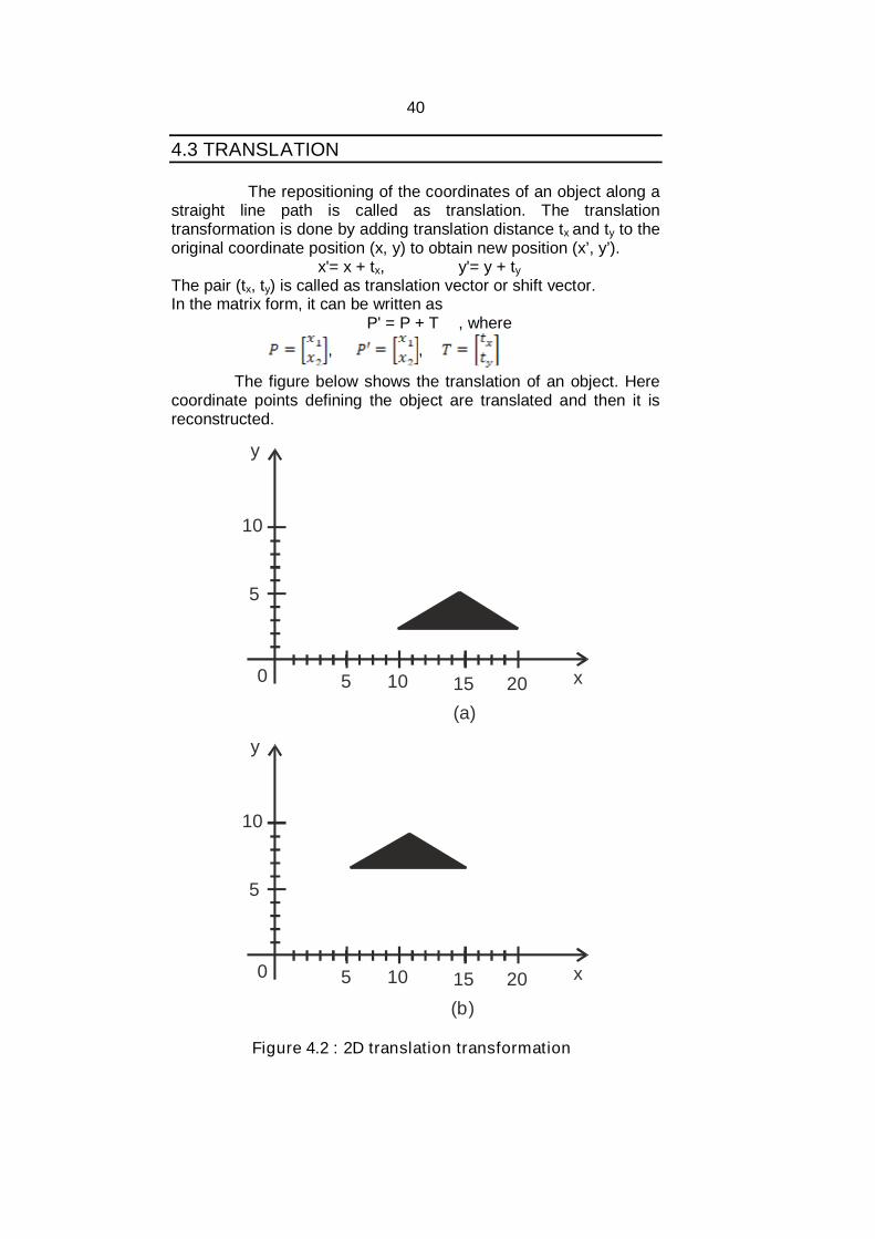
The repositioning of the coordinates of an object along astraight line path is called as translation. The translationtransformation is done by adding translation distance tx and ty to theoriginal coordinate position (x, y) to obtain new position (x’, y’).

x'= x + tx, y'= y + tyThe pair (tx, ty) is called as translation vector or shift vector.In the matrix form, it can be written as

P' = P + T , where

, ,

The figure below shows the translation of an object. Herecoordinate points defining the object are translated and then it isreconstructed.

0

5

10

5 10 15 20

(a)

(b)

x

y

0

5

10

5 10 15 20 x

y

Figure 4.2 : 2D translation transformation

41


1. Translate a triangle with vertices at original coordinates (10, 20),(10,10), (20,10) by tx=5, ty=10.

Answer:1. (15, 30), (15, 20), and (25, 20)

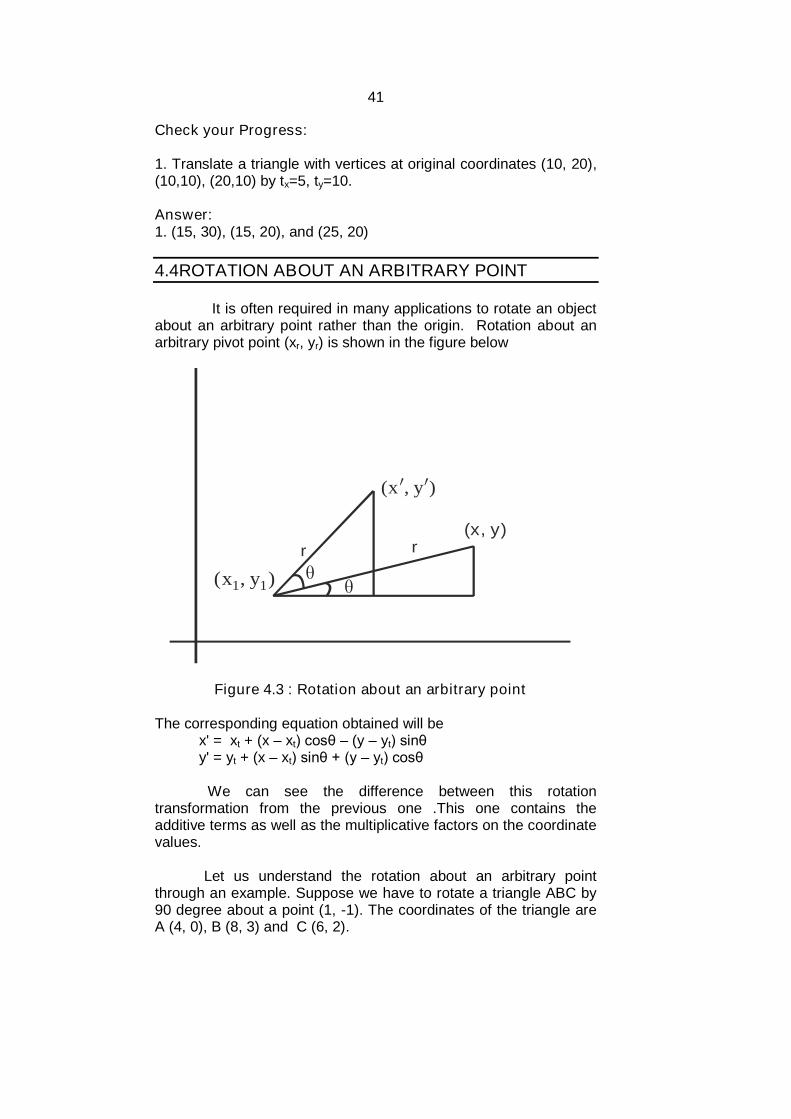
4.4ROTATION ABOUT AN ARBITRARY POINT

It is often required in many applications to rotate an objectabout an arbitrary point rather than the origin. Rotation about anarbitrary pivot point (xr, yr) is shown in the figure below

(x, y)r r

(x , y )¢ ¢

qq

1 1(x , y )

Figure 4.3 : Rotation about an arbitrary point

The corresponding equation obtained will bex' = xt + (x – xt) cosθ – (y – yt) sinθy' = yt + (x – xt) sinθ + (y – yt) cosθ

We can see the difference between this rotationtransformation from the previous one .This one contains theadditive terms as well as the multiplicative factors on the coordinatevalues.

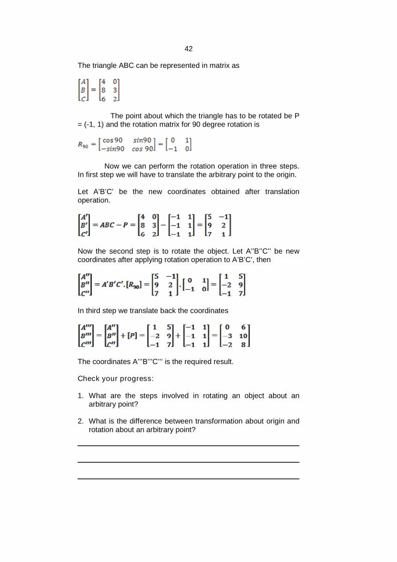
Let us understand the rotation about an arbitrary pointthrough an example. Suppose we have to rotate a triangle ABC by90 degree about a point (1, -1). The coordinates of the triangle areA (4, 0), B (8, 3) and C (6, 2).

42

The triangle ABC can be represented in matrix as

The point about which the triangle has to be rotated be P= (-1, 1) and the rotation matrix for 90 degree rotation is

Now we can perform the rotation operation in three steps.In first step we will have to translate the arbitrary point to the origin.

Let A’B’C’ be the new coordinates obtained after translationoperation.

Now the second step is to rotate the object. Let A’’B’’C’’ be newcoordinates after applying rotation operation to A’B’C’, then

In third step we translate back the coordinates

The coordinates A’’’B’’’C’’’ is the required result.


1. What are the steps involved in rotating an object about anarbitrary point?

2. What is the difference between transformation about origin androtation about an arbitrary point?

43

4.5 COMBINED TRANSFORMATION

A sequence of transformation is said to be as compositeor combined transformations can be represented by product ofmatrices. The product is obtained by multiplying the transformationmatrices in order from right to left.

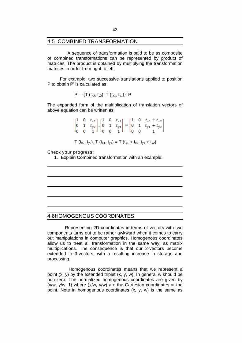
For example, two successive translations applied to positionP to obtain P’ is calculated as

P' = {T (tx2, ty2). T (tx1, ty1)}. P

The expanded form of the multiplication of translation vectors ofabove equation can be written as

T (tx2, ty2). T (tx1, ty1) = T (tx1 + tx2, ty1 + ty2)

Check your progress:1. Explain Combined transformation with an example.

4.6HOMOGENOUS COORDINATES

Representing 2D coordinates in terms of vectors with twocomponents turns out to be rather awkward when it comes to carryout manipulations in computer graphics. Homogenous coordinatesallow us to treat all transformation in the same way, as matrixmultiplications. The consequence is that our 2-vectors becomeextended to 3-vectors, with a resulting increase in storage andprocessing.

Homogenous coordinates means that we represent apoint (x, y) by the extended triplet (x, y, w). In general w should benon-zero. The normalized homogenous coordinates are given by(x/w, y/w, 1) where (x/w, y/w) are the Cartesian coordinates at thepoint. Note in homogenous coordinates (x, y, w) is the same as

44

(x/w, y/w, 1) as is (ax; ay; aw) where a can be any real number.Points with w=0 are called points at infinity, and are not frequentlyused.

Check your progress:1. What is the significance of homogenous coordinates?

4.7 2D TRANSFORMATIONS USING HOMOGENOUSCOORDINATES

The homogenous coordinates for transformations are as follows:For translation

For rotation

For scaling


1. Obtain translation matrix for tx=2, ty=3 in homogenouscoordinate system.

2. Obtain scaling matrix for sx=sy=2 in homogenous coordinatesystem.

45

Answers: 1.

2.

4.8 LET US SUM UP

We learnt the basics of transformation and its use. Then westudied two dimensional transformation and its types which weretranslation, scaling, rotation, reflection and shear. Thetransformation matrix corresponding to each transformationoperation was also studied. Homogenous coordinate system and itsimportance were also discussed.




4.10 EXERCISE

12.Find the new coordinates of the point (2, -4) after the rotation of300.

13.Rotate a triangle about the origin with vertices at originalcoordinates (10, 20), (10, 10), (20, 10) by 30 degrees.

14.Show that successive rotations in two dimensions are additive.

15.Obtain a matrix for two dimensional rotation transformation byan angle θ in clockwise direction.

16.Obtain the transformation matrix to reflect a point A (x, y) aboutthe line y = mx + c.

Answers: 1. (√3+2, 1-2√3)2. (-1.34, 22.32), (3.6, 13.66), and (12.32, 18.66)

46

5

THREE DIMENSIONALTRANSFORMATIONS I

Unit Structure

5.0 Objectives

5.1 Introduction

5.2 Objects in Homogeneous Coordinates

5.3 Transformation Matrix

5.4 Three-Dimensional Transformations

5.5 Scaling

5.6 Translation

5.7 Rotation

5.8 Shear Transformations

5.9 Reflection

5.10 Let us sum up


5.12 Exercise

5.0 OBJECTIVES

The objective of this chapter is To understand the Objects in Homogeneous Coordinates To understand the transformation matrix for 3D transformation. To understand the basics of three- dimensional

transformations To understand the 3D scaling transformation. To understand 3D translation and rotation transformations. To understand 3D shear and reflection transformations.

5.1 INTRODUCTION

In two dimensions there are two perpendicular axes labeledx and y. A coordinate system in three dimensions consists similarlyof three perpendicular axes labeled x, y and z. The third axis makesthe transformation operations different from two dimensions whichwill be discussed in this chapter.

47

5.2 OBJECTS IN HOMOGENOUS COORDINATES

Homogeneous coordinates enables us to perform certainstandard operations on points in Euclidean (XYZ) space by meansof matrix multiplications. In Cartesian coordinate system, a point isrepresented by list ofn points, where n is the dimension of thespace. The homogeneous coordinates corresponding to the samepoint require n+1 coordinates. Thus the two-dimensional point (x, y)becomes (x, y, 1) in homogeneous coordinates, and the three-dimensional point (x, y, z) becomes (x, y, z, 1). The same conceptcan be applied to higher dimensions. For example, Homogeneouscoordinates in a seven-dimensional Euclidean space have eightcoordinates.

In combined transformation, a translation matrix can becombined with a translation matrix, a scaling matrix with a scalingmatrix and similarly a rotation matrix with a rotation matrix. Thescaling matrices and rotation matrices can also be combined asboth of them are 3x3 matrices. If we want to combine a translationmatrix with a scaling matrix and/or a rotation matrix, we will firsthave to change the translation matrix in homogenous coordinatesystem.

Further in three dimensional, for uniform transformation weneed to add a component to the vectors and increase thedimension of the transformation matrices. This for componentsrepresentation is known as homogenous coordinate representation.

5.3THREE DIMENSIONAL TRANSFORMATIONS

The transformations procedure in three dimensions is similarto transformations in two dimensions. 3D Affine Transformation:

A coordinate transformation of the form:x' = axx x + axy y + axz z + bx ,y' = ayx x + ayy y + ayz z + by ,z' = azx x + azy y + azz z + bz ,

is called a 3D affine transformation. It can also berepresented by transformation matrix as given below

11000

'

'

'

z

y

x

baaa

baaa

baaa

w

z

y

x

zzzzyzx

yyzyyyx

xxzxyxx

48

o Translation, scaling, shearing, rotation (or any combinationsof them) are examples affine transformations.

o Lines and planes are preserved.

o Parallelism of lines and planes are also preserved, but notangles and length.

Object transformation:Objects can be transformed using 2D and 3D transformationtechniques

Line: Lines can be transformed by transforming the endpoints.

Plane (described by 3-points):It can be transformed bytransforming the 3-points.

Plane (described by a point and normal): Point istransformed as usual. Special treatment is needed fortransforming normal.

Check your progress:1. Explain 3D affine transformation.2. Explain object transformation.

5.4 SCALING

Scaling transformation changes the dimension of a 3D objectdetermined by scale factors in all three directions.

x' = x. sx y' = y. sy z' = z. sz

The transformation matrix and scaling through it

49

Check your Progress:1. Explain the scaling process in three dimension.2. Derive scaling matrix with sx=sy=2 and sz=1.

Answer: 2.

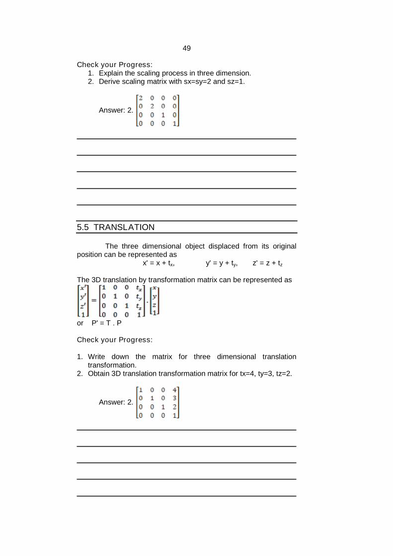
5.5 TRANSLATION

The three dimensional object displaced from its originalposition can be represented as

x' = x + tx, y' = y + ty, z' = z + tz

The 3D translation by transformation matrix can be represented as

or P' = T . P


1. Write down the matrix for three dimensional translationtransformation.

2. Obtain 3D translation transformation matrix for tx=4, ty=3, tz=2.

Answer: 2.

50

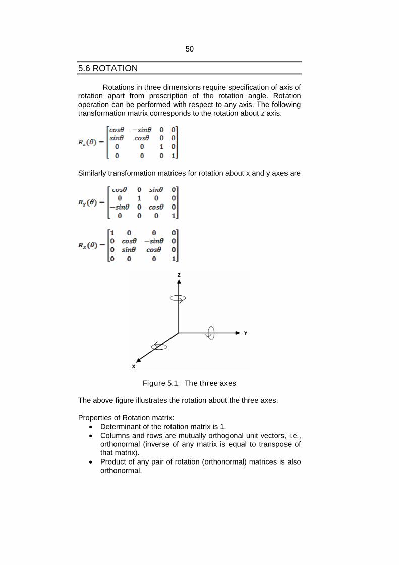
5.6 ROTATION

Rotations in three dimensions require specification of axis ofrotation apart from prescription of the rotation angle. Rotationoperation can be performed with respect to any axis. The followingtransformation matrix corresponds to the rotation about z axis.

Similarly transformation matrices for rotation about x and y axes are

Figure 5.1: The three axes

The above figure illustrates the rotation about the three axes.

Properties of Rotation matrix: Determinant of the rotation matrix is 1. Columns and rows are mutually orthogonal unit vectors, i.e.,

orthonormal (inverse of any matrix is equal to transpose ofthat matrix).

Product of any pair of rotation (orthonormal) matrices is alsoorthonormal.

51

Check your progress:1. Explain three dimensional rotation transformation.2. Derive the three dimensional rotation matrix about y axis with

rotation angle 90 degrees.

Answer: 2.

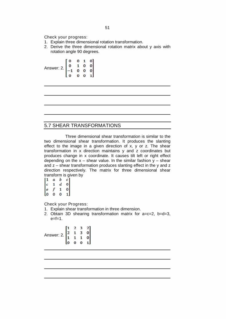
5.7 SHEAR TRANSFORMATIONS

Three dimensional shear transformation is similar to thetwo dimensional shear transformation. It produces the slantingeffect to the image in a given direction of x, y or z. The sheartransformation in x direction maintains y and z coordinates butproduces change in x coordinate. It causes tilt left or right effectdepending on the x – shear value. In the similar fashion y – shearand z – shear transformation produces slanting effect in the y and zdirection respectively. The matrix for three dimensional sheartransform is given by

Check your Progress:1. Explain shear transformation in three dimension.2. Obtain 3D shearing transformation matrix for a=c=2, b=d=3,

e=f=1.

Answer: 2.

52

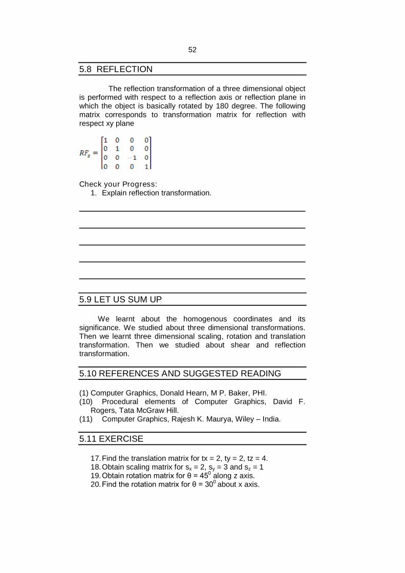
5.8 REFLECTION

The reflection transformation of a three dimensional objectis performed with respect to a reflection axis or reflection plane inwhich the object is basically rotated by 180 degree. The followingmatrix corresponds to transformation matrix for reflection withrespect xy plane

Check your Progress:1. Explain reflection transformation.

5.9 LET US SUM UP

We learnt about the homogenous coordinates and itssignificance. We studied about three dimensional transformations.Then we learnt three dimensional scaling, rotation and translationtransformation. Then we studied about shear and reflectiontransformation.


(1) Computer Graphics, Donald Hearn, M P. Baker, PHI.(10) Procedural elements of Computer Graphics, David F.

Rogers, Tata McGraw Hill.(11) Computer Graphics, Rajesh K. Maurya, Wiley – India.

5.11 EXERCISE

17.Find the translation matrix for tx = 2, ty = 2, tz = 4.18.Obtain scaling matrix for sx = 2, sy = 3 and sz = 119.Obtain rotation matrix for θ = 450 along z axis.20.Find the rotation matrix for θ = 300 about x axis.

53

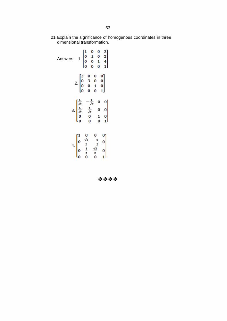
21.Explain the significance of homogenous coordinates in threedimensional transformation.

Answers: 1.

2.

3.

4.

54

6

THREE DIMENSIONALTRANSFORMATIONS II

Unit Structure6.0 Objectives6.1 Introduction6.2 World Coordinates and Viewing Coordinates6.3 Projection6.4 Parallel Projection6.5 Perspective Projection6.6 Let us sum up6.7 References and Suggested Reading6.8 Exercise

6.0 OBJECTIVES

The objective of this chapter is to understand World Coordinates and Viewing Coordinates Projection transformation – Parallel projections and

perspective projection

6.1 INTRODUCTION

Projections help us to represent a three dimensional objectinto two dimensional plane. It is basically mapping of a point ontoits image in the view plane or projection plane. There are differenttypes of projection techniques. In this chapter we are going todiscuss the basic idea of projection.

6.2 WORLD COORDINATES AND VIEWINGCOORDINATES

Objects in general are said to be specified by the coordinatesystem known as world coordinate system (WCS). Sometimes itis required to select a portion of the scene in which the objects areplaced. This portion is captured by a rectangular area whose edgesare parallel to the axes of the WCS and is known as window.

55

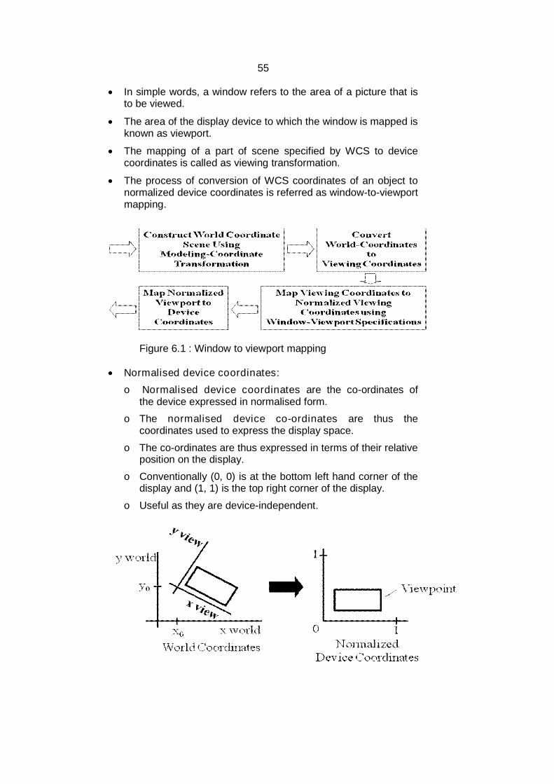
In simple words, a window refers to the area of a picture that isto be viewed.

The area of the display device to which the window is mapped isknown as viewport.

The mapping of a part of scene specified by WCS to devicecoordinates is called as viewing transformation.

The process of conversion of WCS coordinates of an object tonormalized device coordinates is referred as window-to-viewportmapping.

Figure 6.1 : Window to viewport mapping

Normalised device coordinates:

o Normalised device coordinates are the co-ordinates ofthe device expressed in normalised form.

o The normalised device co-ordinates are thus thecoordinates used to express the display space.

o The co-ordinates are thus expressed in terms of their relativeposition on the display.

o Conventionally (0, 0) is at the bottom left hand corner of thedisplay and (1, 1) is the top right corner of the display.

o Useful as they are device-independent.

56

Figure 6.2: World coordinates and normalized devicecoordinate

Check your progress:1. A rectangular area whose edges are parallel to the axes of the

WCS and is known as.............

2. Define normalised device coordinates.

Answers: 1. window

6.3 PROJECTION

Projection is the process of representing a 3D object onto a2D screen. It is basically a mapping of any point P (x, y, z) to itsimage P (x’, y’, z’) onto a plane called as projection plane. Theprojection transformation can be broadly classified into twocategories: Parallel and Perspective projections.

6.4 PARALLEL PROJECTION

In parallel projections the lines of projection are parallel bothin reality and in the projection plane. The orthographic projection isone of the most widely used parallel projections.

Orthographic projection: Orthographic projection utilizesperpendicular projectors from the object to a plane of projection togenerate a system of drawing views.

These projections are used to describe the design and featuresof an object.

It is one of the parallel projection form, all the projection linesare orthogonal to the projection plane.

57

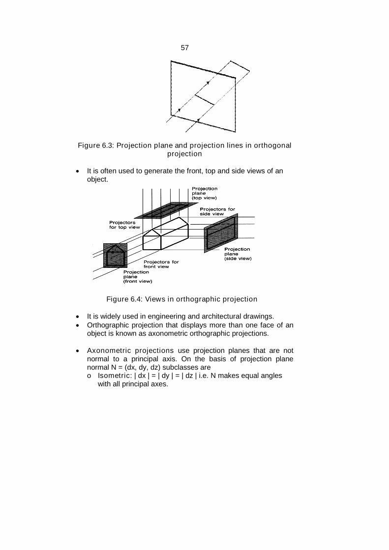
Figure 6.3: Projection plane and projection lines in orthogonalprojection

It is often used to generate the front, top and side views of anobject.

Figure 6.4: Views in orthographic projection

It is widely used in engineering and architectural drawings. Orthographic projection that displays more than one face of an

object is known as axonometric orthographic projections.

Axonometric projections use projection planes that are notnormal to a principal axis. On the basis of projection planenormal N = (dx, dy, dz) subclasses areo Isometric: | dx | = | dy | = | dz | i.e. N makes equal angles

with all principal axes.

58

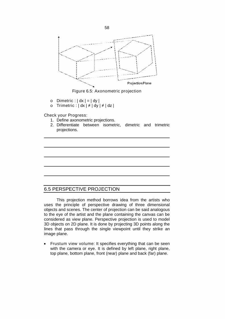
Figure 6.5: Axonometric projection

o Dimetric : | dx | = | dy |o Trimetric : | dx | ≠ | dy | ≠ | dz |

Check your Progress:1. Define axonometric projections.2. Differentiate between isometric, dimetric and trimetric

projections.

6.5 PERSPECTIVE PROJECTION

This projection method borrows idea from the artists whouses the principle of perspective drawing of three dimensionalobjects and scenes. The center of projection can be said analogousto the eye of the artist and the plane containing the canvas can beconsidered as view plane. Perspective projection is used to model3D objects on 2D plane. It is done by projecting 3D points along thelines that pass through the single viewpoint until they strike animage plane.

Frustum view volume: It specifies everything that can be seenwith the camera or eye. It is defined by left plane, right plane,top plane, bottom plane, front (near) plane and back (far) plane.

59

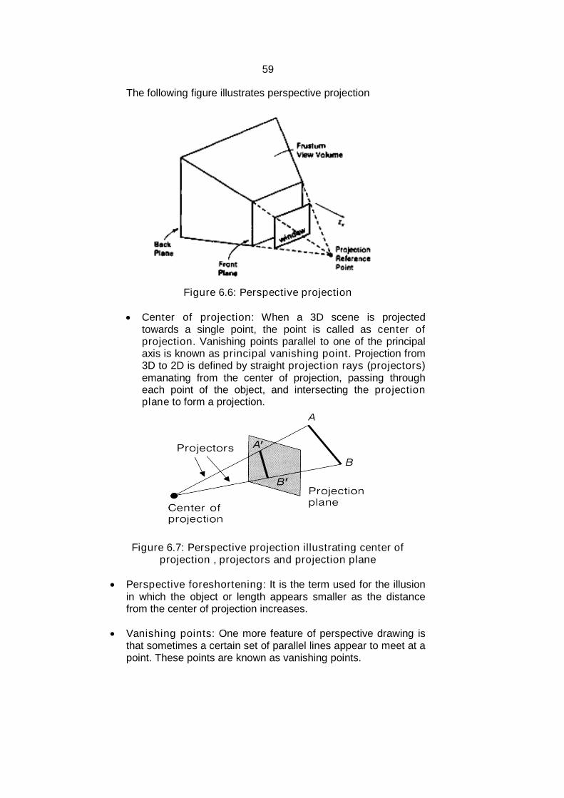
The following figure illustrates perspective projection

Figure 6.6: Perspective projection

Center of projection: When a 3D scene is projectedtowards a single point, the point is called as center ofprojection. Vanishing points parallel to one of the principalaxis is known as principal vanishing point. Projection from3D to 2D is defined by straight projection rays (projectors)emanating from the center of projection, passing througheach point of the object, and intersecting the projectionplane to form a projection.

Figure 6.7: Perspective projection illustrating center ofprojection , projectors and projection plane

Perspective foreshortening: It is the term used for the illusionin which the object or length appears smaller as the distancefrom the center of projection increases.

Vanishing points: One more feature of perspective drawing isthat sometimes a certain set of parallel lines appear to meet at apoint. These points are known as vanishing points.

60

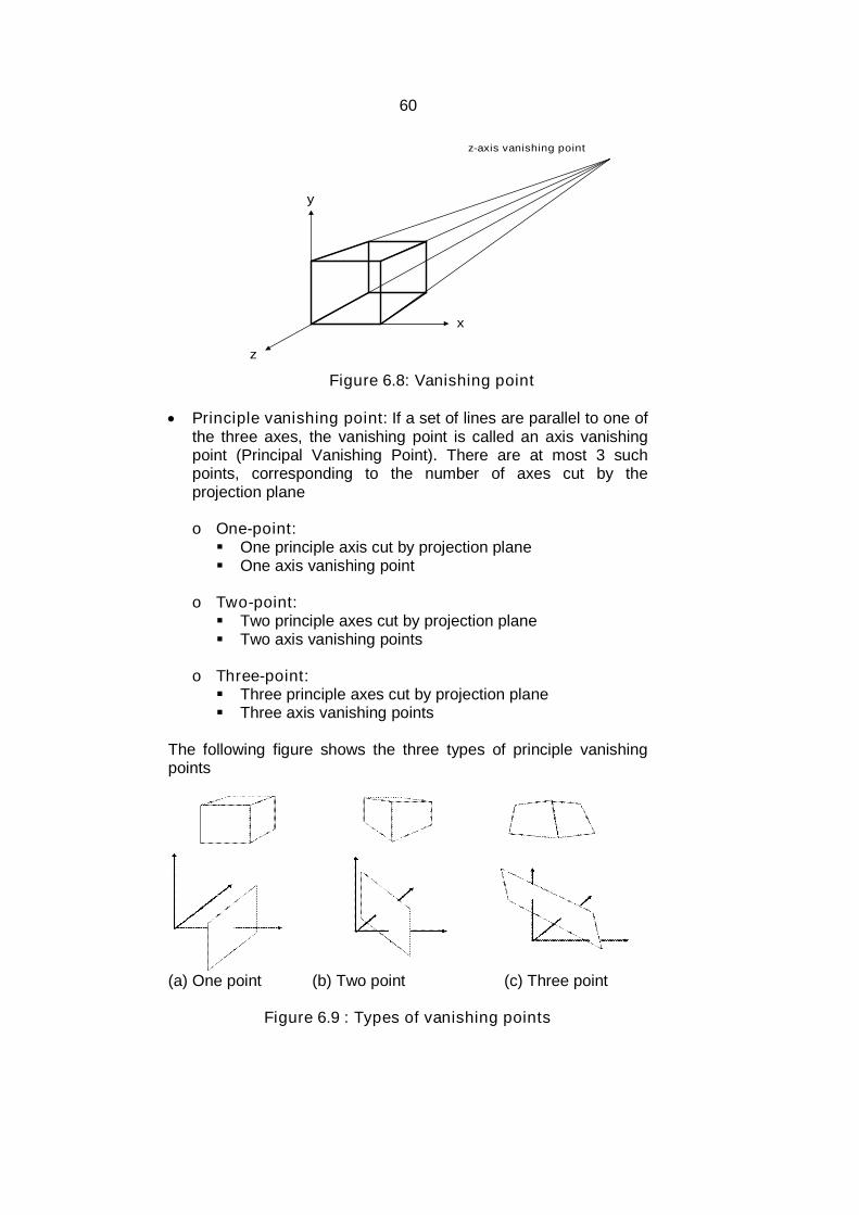
Figure 6.8: Vanishing point

Principle vanishing point: If a set of lines are parallel to one ofthe three axes, the vanishing point is called an axis vanishingpoint (Principal Vanishing Point). There are at most 3 suchpoints, corresponding to the number of axes cut by theprojection plane

o One-point: One principle axis cut by projection plane One axis vanishing point

o Two-point: Two principle axes cut by projection plane Two axis vanishing points

o Three-point: Three principle axes cut by projection plane Three axis vanishing points

The following figure shows the three types of principle vanishingpoints

(a) One point (b) Two point (c) Three point

Figure 6.9 : Types of vanishing points

x

y

z

z-axis vanishing point

61

View confusion: Objects behind the center of projection areprojected upside down and backward onto the view plane.

Topological distortion: A line segment joining a point whichlies in front of the viewer to a point in back of the viewer isprojected to a broken line of infinite extent.

Check your progress:1. Define centre of projection.2. What is the term used for the illusion in which the object or

length appears smaller as the distance from the center ofprojection increases?

Answer: 2. Perspective foreshortening

6.6 LET US SUM UP

In this chapter we learnt about world coordinate system andview coordinates. We then learnt the fundamental definition ofprojection. Orthographic projection with its application wasdiscussed in short. We then learnt perspective projection and termsassociated with it.


(1) Computer Graphics, Donald Hearn, M P. Baker, PHI.(12) Procedural elements of Computer Graphics, David F.

Rogers, Tata McGraw Hill.(13) Computer Graphics, Rajesh K. Maurya, Wiley – India.

6.8 EXERCISE

1. Explain world coordinate system.2. Define viewing coordinates.3. Explain orthographic projection with its applications.4. What is topological distortion?5. Describe perspective projection and explain perspectiveforeshortening and vanishing points.

62

7

VIEWING AND SOLID AREA SCAN-CONVERSION

Unit Structure:

7.0 Objectives7.1 Introduction to viewing and clipping7.2 Viewing Transformation in Two Dimensions7.3 Introduction to Clipping:

7.3.1 Point Clipping7.3.2 Line Clipping

7.4 Introduction to a Polygon Clipping7.5 Viewing and Clipping in Three Dimensions7.6 Three-Dimensional Viewing Transformations7.7 Text Clipping7.8 Let us sum up


7.10 Exercise

7.0 OBJECTIVES

The objective of this chapter is

To understand the basics of concept of viewing transformations. To understand point clipping, line clipping and polygon clipping To understand the concept of text clipping.

7.1 INTRODUCTION TO VIEWING AND CLIPPING

Windowing and clippingA “picture” is a “scene” consists of different objects.

The individual objects are represented by coordinates calledas “model” or “local” or ”master” coordinates.

The objects are fitted together to create a picture, using co-ordinates called a word coordinate (WCS).

63

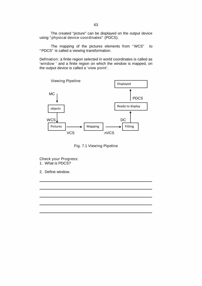
The created “picture” can be displayed on the output deviceusing “physical device coordinates” (PDCS).

The mapping of the pictures elements from “WCS” to“PDCS” is called a viewing transformation.

Defination: a finite region selected in world coordinates is called as‘window ’ and a finite region on which the window is mapped, onthe output device is called a ‘view point’.

Viewing Pipeline

MCPDCS

WCS DC

VCS nVCS

Fig. 7.1 Viewing Pipeline

Check your Progress:1. What is PDCS?

2. Define window.

objects

Pictures Mapping Fitting

Ready to display

Displayed

64

7.2 VIEWING TRANSFORMATION IN TWODIMENSIONS

Viewing Transformation / a complete mapping from window toview point.

Window

ywmax

ywmin

Xwmin xwmax

View port

yvmax

yvmin

Xvmin xvmax

Let W in window defined

by the lines:

x= xwmin, x=xwmax,

y=ywmin, y=ywmax

Then the aspect ratio for

w defined by,

aw= (xwamx –xwmin) /

(ywmax- ywmin)

similarly for a view port

say V we have,

av= (xvmax-xvmin) /

(yvmax- yvmin)

Fig. 7.2 Window and Viewpoint

7.3 INTRODUCTION TO CLIPPING

The process which divides the given picture into two parts :visible and Invisible and allows to discard the invisible part is knownas clipping. For clipping we need reference window called asclipping window.

(Xmax,Ymax)

(Xmin, Ymin)

Fig. 7.3 Window

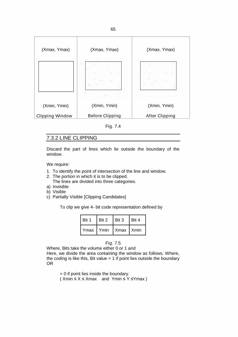
7.3.1 POINT CLIPPING

Discard the points which lie outside the boundary of the clippingwindow. Where,Xmin ≤ X ≤ Xmax andYmin ≤ Y ≤Ymax

WV

65

(Xmax, Ymax)

(Xmin, Ymin)

Clipping Window

(Xmax, Ymax)

(Xmin, Ymin)

Before Clipping

(Xmax, Ymax)

(Xmin, Ymin)

After Clipping

Fig. 7.4

7.3.2 LINE CLIPPING

Discard the part of lines which lie outside the boundary of thewindow.

We require:

1. To identify the point of intersection of the line and window.2. The portion in which it is to be clipped.

The lines are divided into three categories.a) Invisibleb) Visiblec) Partially Visible [Clipping Candidates]

To clip we give 4- bit code representation defined by

Bit 1 Bit 2 Bit 3 Bit 4

Ymax Ymin Xmax Xmin

Fig. 7.5Where, Bits take the volume either 0 or 1 andHere, we divide the area containing the window as follows. Where,the coding is like this, Bit value = 1 if point lies outside the boundaryOR

= 0 if point lies inside the boundary.( Xmin ≤ X ≤ Xmax and Ymin ≤ Y ≤Ymax )

66

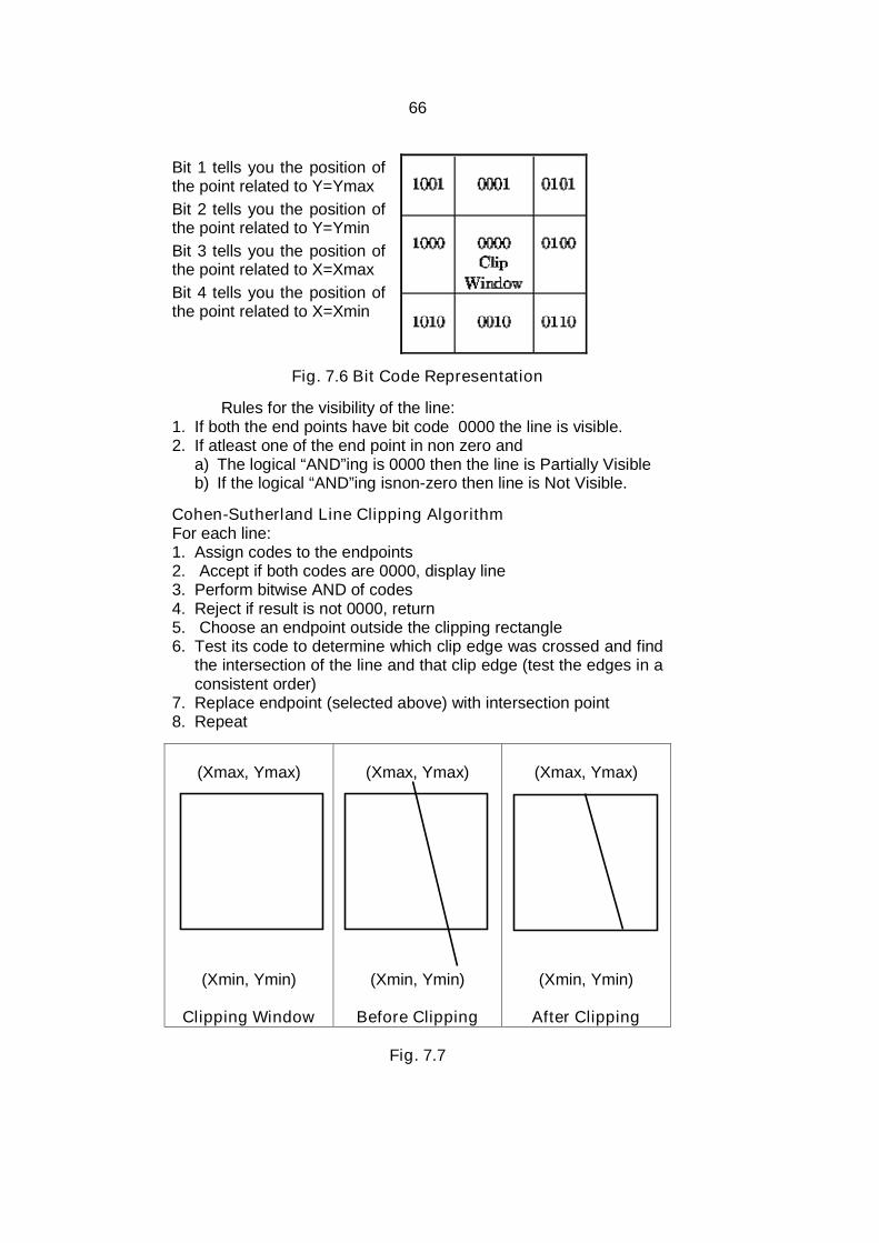
Bit 1 tells you the position ofthe point related to Y=Ymax

Bit 2 tells you the position ofthe point related to Y=Ymin

Bit 3 tells you the position ofthe point related to X=Xmax

Bit 4 tells you the position ofthe point related to X=Xmin

Fig. 7.6 Bit Code Representation

Rules for the visibility of the line:1. If both the end points have bit code 0000 the line is visible.2. If atleast one of the end point in non zero and

a) The logical “AND”ing is 0000 then the line is Partially Visibleb) If the logical “AND”ing isnon-zero then line is Not Visible.

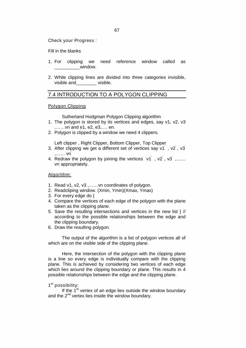
Cohen-Sutherland Line Clipping AlgorithmFor each line:1. Assign codes to the endpoints2. Accept if both codes are 0000, display line3. Perform bitwise AND of codes4. Reject if result is not 0000, return5. Choose an endpoint outside the clipping rectangle6. Test its code to determine which clip edge was crossed and find

the intersection of the line and that clip edge (test the edges in aconsistent order)

7. Replace endpoint (selected above) with intersection point8. Repeat

(Xmax, Ymax)

(Xmin, Ymin)

Clipping Window

(Xmax, Ymax)

(Xmin, Ymin)

Before Clipping

(Xmax, Ymax)

(Xmin, Ymin)

After Clipping

Fig. 7.7

67

Check your Progress :

Fill in the blanks

1. For clipping we need reference window called as__________window.

2. While clipping lines are divided into three categories invisible,visible and________ visible.

7.4 INTRODUCTION TO A POLYGON CLIPPING

Polygon Clipping

Sutherland Hodgman Polygon Clipping algorithm1. The polygon is stored by its vertices and edges, say v1, v2, v3

,……vn and e1, e2, e3,…. en.2. Polygon is clipped by a window we need 4 clippers.

Left clipper , Right Clipper, Bottom Clipper, Top Clipper3. After clipping we get a different set of vertices say v1’ , v2’ , v3’

,…… vn’

4. Redraw the polygon by joining the vertices v1’ , v2’ , v3’ ,……vn’ appropriately.

Algorithm:

1. Read v1, v2, v3 ,……vn coordinates of polygon.2. Readcliping window. (Xmin, Ymin)(Xmax, Ymax)3. For every edge do {4. Compare the vertices of each edge of the polygon with the plane

taken as the clipping plane.5. Save the resulting intersections and vertices in the new list } //

according to the possible relationships between the edge andthe clipping boundary.

6. Draw the resulting polygon.

The output of the algorithm is a list of polygon vertices all ofwhich are on the visible side of the clipping plane.

Here, the intersection of the polygon with the clipping planeis a line so every edge is individually compare with the clippingplane. This is achieved by considering two vertices of each edgewhich lies around the clipping boundary or plane. This results in 4possible relationships between the edge and the clipping plane.

1st possibility:If the 1st vertex of an edge lies outside the window boundary

and the 2nd vertex lies inside the window boundary.

68

Here, point of intersection of the edge with the windowboundaryand the second vertex are added to the putput vertex list(V1, v2)→( V1’, v2)

V1V1’ V2

Fig. 7.8

2nd possibility:If both the vertices of an edge are inside of the window

boundary only the second vertex is added to the vertex list

Fig. 7.9

3rd possibility:If the 1st vertex is inside the window and 2nd vertex is outside

only the intersection point is add to the output vertex list.

V1V2’ V2 v3’ v4

V3

Fig. 7.10

4th possibility:If both vertices are outside the window nothing is added to

the vertex list.

Once all vertices are processed for one clipped boundarythen the output list of vertices is clipped against the next windowboundary going through above 4 possibilities. We have to considerthe following points.

1) The visibility of the point. We apply inside-outside test.2) Finding intersection of the edge with the clipping plane.

69

7.5 VIEWING AND CLIPPING IN THREE DIMENSIONS

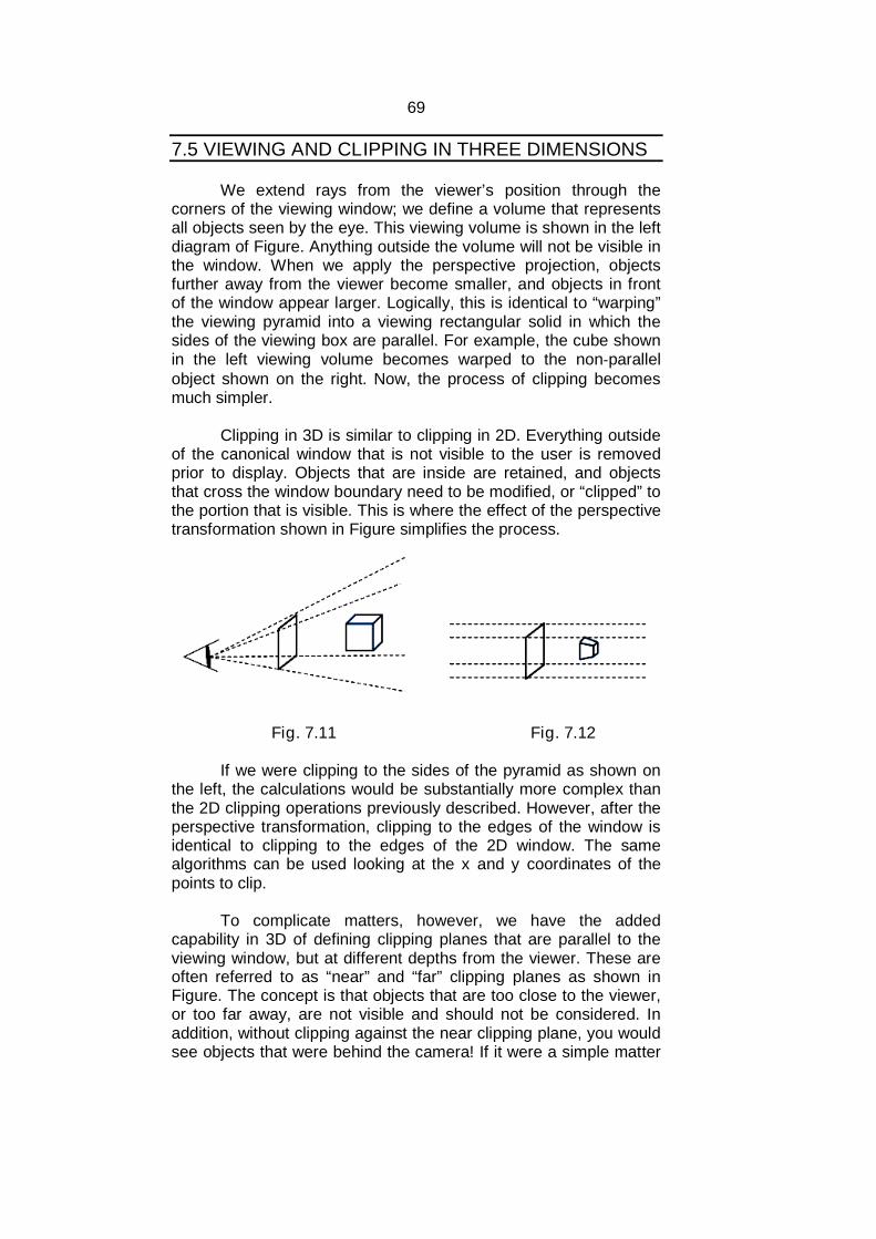
We extend rays from the viewer’s position through thecorners of the viewing window; we define a volume that representsall objects seen by the eye. This viewing volume is shown in the leftdiagram of Figure. Anything outside the volume will not be visible inthe window. When we apply the perspective projection, objectsfurther away from the viewer become smaller, and objects in frontof the window appear larger. Logically, this is identical to “warping”the viewing pyramid into a viewing rectangular solid in which thesides of the viewing box are parallel. For example, the cube shownin the left viewing volume becomes warped to the non-parallelobject shown on the right. Now, the process of clipping becomesmuch simpler.

Clipping in 3D is similar to clipping in 2D. Everything outsideof the canonical window that is not visible to the user is removedprior to display. Objects that are inside are retained, and objectsthat cross the window boundary need to be modified, or “clipped” tothe portion that is visible. This is where the effect of the perspectivetransformation shown in Figure simplifies the process.

Fig. 7.11 Fig. 7.12

If we were clipping to the sides of the pyramid as shown onthe left, the calculations would be substantially more complex thanthe 2D clipping operations previously described. However, after theperspective transformation, clipping to the edges of the window isidentical to clipping to the edges of the 2D window. The samealgorithms can be used looking at the x and y coordinates of thepoints to clip.

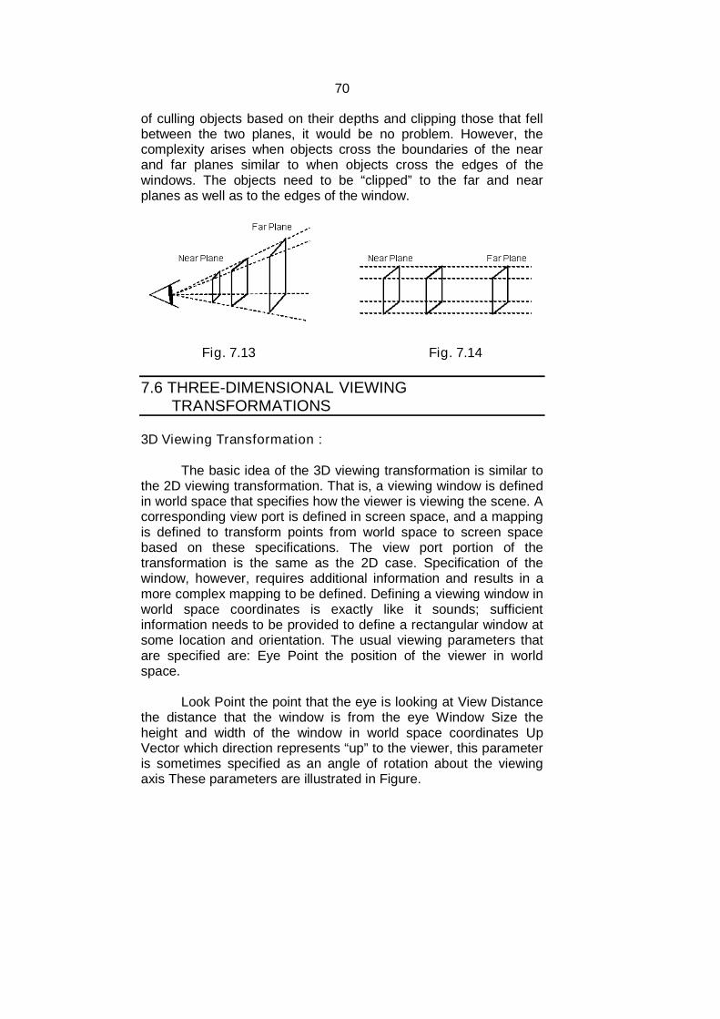
To complicate matters, however, we have the addedcapability in 3D of defining clipping planes that are parallel to theviewing window, but at different depths from the viewer. These areoften referred to as “near” and “far” clipping planes as shown inFigure. The concept is that objects that are too close to the viewer,or too far away, are not visible and should not be considered. Inaddition, without clipping against the near clipping plane, you wouldsee objects that were behind the camera! If it were a simple matter

70

of culling objects based on their depths and clipping those that fellbetween the two planes, it would be no problem. However, thecomplexity arises when objects cross the boundaries of the nearand far planes similar to when objects cross the edges of thewindows. The objects need to be “clipped” to the far and nearplanes as well as to the edges of the window.

Fig. 7.13 Fig. 7.14

7.6 THREE-DIMENSIONAL VIEWINGTRANSFORMATIONS

3D Viewing Transformation :

The basic idea of the 3D viewing transformation is similar tothe 2D viewing transformation. That is, a viewing window is definedin world space that specifies how the viewer is viewing the scene. Acorresponding view port is defined in screen space, and a mappingis defined to transform points from world space to screen spacebased on these specifications. The view port portion of thetransformation is the same as the 2D case. Specification of thewindow, however, requires additional information and results in amore complex mapping to be defined. Defining a viewing window inworld space coordinates is exactly like it sounds; sufficientinformation needs to be provided to define a rectangular window atsome location and orientation. The usual viewing parameters thatare specified are: Eye Point the position of the viewer in worldspace.

Look Point the point that the eye is looking at View Distancethe distance that the window is from the eye Window Size theheight and width of the window in world space coordinates UpVector which direction represents “up” to the viewer, this parameteris sometimes specified as an angle of rotation about the viewingaxis These parameters are illustrated in Figure.

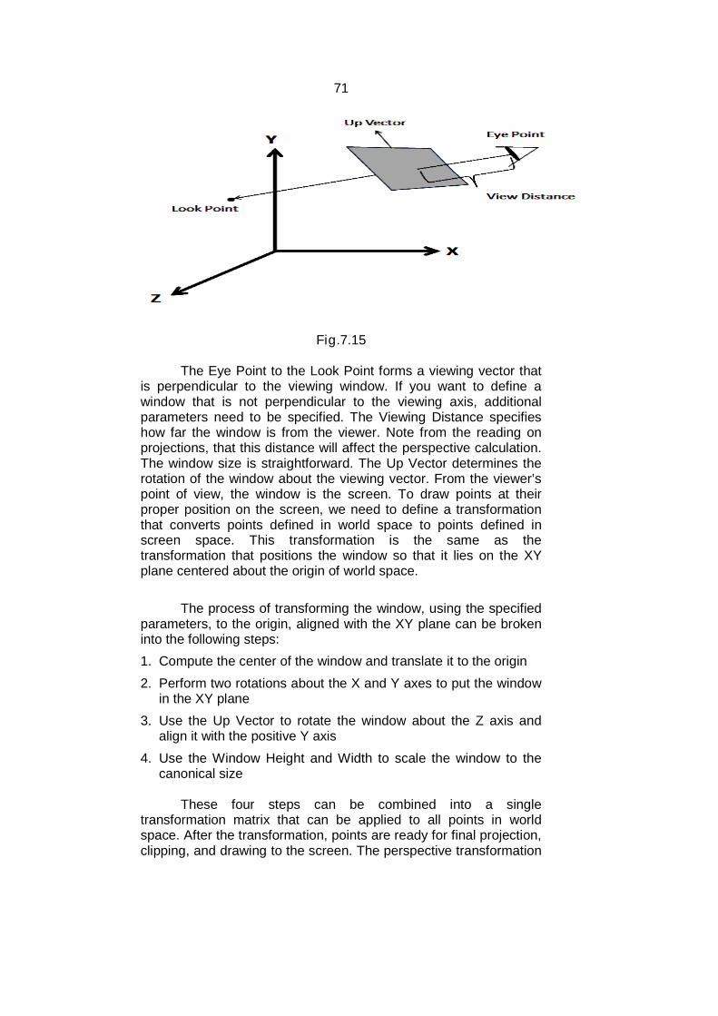
71

Fig.7.15

The Eye Point to the Look Point forms a viewing vector thatis perpendicular to the viewing window. If you want to define awindow that is not perpendicular to the viewing axis, additionalparameters need to be specified. The Viewing Distance specifieshow far the window is from the viewer. Note from the reading onprojections, that this distance will affect the perspective calculation.The window size is straightforward. The Up Vector determines therotation of the window about the viewing vector. From the viewer’spoint of view, the window is the screen. To draw points at theirproper position on the screen, we need to define a transformationthat converts points defined in world space to points defined inscreen space. This transformation is the same as thetransformation that positions the window so that it lies on the XYplane centered about the origin of world space.

The process of transforming the window, using the specifiedparameters, to the origin, aligned with the XY plane can be brokeninto the following steps:

1. Compute the center of the window and translate it to the origin

2. Perform two rotations about the X and Y axes to put the windowin the XY plane

3. Use the Up Vector to rotate the window about the Z axis andalign it with the positive Y axis

4. Use the Window Height and Width to scale the window to thecanonical size

These four steps can be combined into a singletransformation matrix that can be applied to all points in worldspace. After the transformation, points are ready for final projection,clipping, and drawing to the screen. The perspective transformation

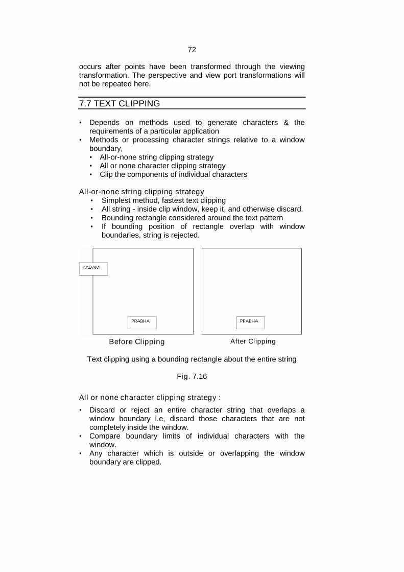
72

occurs after points have been transformed through the viewingtransformation. The perspective and view port transformations willnot be repeated here.

7.7 TEXT CLIPPING

• Depends on methods used to generate characters & therequirements of a particular application

• Methods or processing character strings relative to a windowboundary,• All-or-none string clipping strategy• All or none character clipping strategy• Clip the components of individual characters

All-or-none string clipping strategy• Simplest method, fastest text clipping• All string - inside clip window, keep it, and otherwise discard.• Bounding rectangle considered around the text pattern• If bounding position of rectangle overlap with window

boundaries, string is rejected.

Before Clipping After Clipping

Text clipping using a bounding rectangle about the entire string

Fig. 7.16

All or none character clipping strategy :

• Discard or reject an entire character string that overlaps awindow boundary i.e, discard those characters that are notcompletely inside the window.

• Compare boundary limits of individual characters with thewindow.

• Any character which is outside or overlapping the windowboundary are clipped.

73


Text clipping using a bounding rectangle about individualcharacters

Fig. 7.17

Clip the components of individual characters :• Treat characters same as lines• If individual char overlaps a clip window boundary, clip off the

parts of the character that are outside the window


Text clipping is performed on the components of individualcharacters.

Fig. 7.18

74

Check your Progress:True or False.

1. The perspective and viewport transformations will not berepeated in3D Viewing Transformation.

2. In Sutherland Hodgman Polygon Clipping algorithm polygon isclipped by a window we need 4 clippers.

3. To check the visibility of the point, we apply inside-outside test.

7.8 LET US SUM UP

Point clipping, line clipping, polygon clipping and text clippingare types of the clipping.

Normally window and view points are ‘rectangular’ shaped. The viewing transformation is also called as windowing

transformation. Discarding and removing the invisible region of object from the

given window is known as clipping.

7. 9 REFERENCES AND SUGGESTED READING

Computer Graphics, Donald Hearn, M P. Baker, PHI. Procedural elements of Computer Graphics, David F. Rogers,

Tata McGraw Hill. Computer Graphics, Amarendra Sinha, A. Udai,, Tata McGraw

Hill. Computer Graphics,A. P. Godase, Technical Publications Pune.

7.10 EXERCISE

1. What is point clipping?2. Explain Cohen-Sutherland Line clipping algorithm.3. Explain the polygon clipping algorithm.4. Write a short note on text clipping.5. Define: window, View point.

75

8

INTRODUCTION TO SOLID AREA SCAN-CONVERSION

Unit Structure:

8.0 Objectives8.1 Introduction8.2 Inside–Outside Test8.3 Winding Number Method and Coherence Property8.4 Polygon Filling and Seed Fill Algorithm8.5 Scan-Line Algorithm8.6 Priority Algorithm8.7 Scan Conversion of Character8.8 Aliasing, Anti-Aliasing, Half toning8.9 Thresholding and Dithering8.10 Let us sum up8.11 References and Suggested Reading8.12 Exercise

8.0 OBJECTIVE

The objective of this chapter is To understand polygon filling techniques and algorithms. To understand scan conversion of characters. To understand concepts of anti-alising, half toning, thresholding

and diathering.

8.1 INTRODUCTION

To perform the scan conversion or to fill the polygon, weneed the pixels inside the polygon as well as those on theboundary. The pixels which are inside the polygon can bedetermined by using the following two test: Inside outside test andWinding number test.

8.2 INSIDE–OUTSIDE TEST

1. Inside outside test (Even- Odd Test)

We assume that the vertex list for the polygon is alreadystored and proceed as follows.

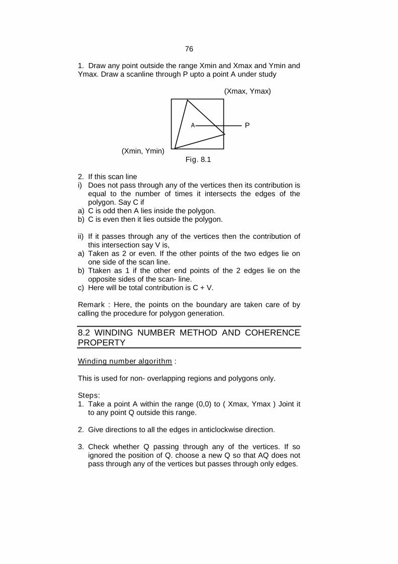
76

1. Draw any point outside the range Xmin and Xmax and Ymin andYmax. Draw a scanline through P upto a point A under study

(Xmax, Ymax)

P

(Xmin, Ymin)Fig. 8.1

2. If this scan linei) Does not pass through any of the vertices then its contribution is

equal to the number of times it intersects the edges of thepolygon. Say C if

a) C is odd then A lies inside the polygon.b) C is even then it lies outside the polygon.

ii) If it passes through any of the vertices then the contribution ofthis intersection say V is,

a) Taken as 2 or even. If the other points of the two edges lie onone side of the scan line.

b) Ttaken as 1 if the other end points of the 2 edges lie on theopposite sides of the scanline.

c) Here will be total contribution is C + V.

Remark : Here, the points on the boundary are taken care of bycalling the procedure for polygon generation.

8.2 WINDING NUMBER METHOD AND COHERENCEPROPERTY

Winding number algorithm :

This is used for non- overlapping regions and polygons only.

Steps:1. Take a point A within the range (0,0) to ( Xmax, Ymax ) Joint it

to any point Q outside this range.

2. Give directions to all the edges in anticlockwise direction.

3. Check whether Q passing through any of the vertices. If soignored the position of Q. choose a new Q so that AQ does notpass through any of the vertices but passes through only edges.

A

77

(Xmax, Ymax) AQ is passing through edges.

Q

(0,0)

w=0Subtract 1 from w, if crossesedge moves from left to right:w= 0-1= -1w is non zero so A lies insidethe polygon.

4. Initialize winding number w=0. Observe the edges intersectingAQ and

1) Add 1 to w if cross edge moves from right to left2) Subtract 1 from w, if crosses edge moves from left to right.

5. If final count of w is zero1) A lies outside the polygon2) Non zero, A lies inside the polygon.3) Illuminate the interior position till all the pixels in the above set

range are painted.

8.3 POLYGON FILLING AND SEED FILL ALGORITHM

Polygon filling algorithm

There are two types of polygon filling algorithm.1. Scan conversion polygon filling algorithm2. Seed filling algorithms

Besides these algorithms we can usea) Boundary fill algorithms andb) Flood fill algorithm

Seed Fill

To fill a polygon we start with a seed and point theneighboring points till the boundary of the polygon is reached. Ifboundary pixels are not reaching pixels are illuminated one by oneand the process is continuing until the boundary points arereached. Here, at every step we need check the boundary. Hence,this algorithm is called “boundary fill algorithm”.

To find the neighboring pixels we can use either a 4connected or 8 connected region filling algorithm.

A

78

The algorithm is recursive one and can be given as follows:

Here, we specify the parameters, fore-color by F and back-color by B

4 Neighbors are:N4={ (X+1,Y), (X-1,Y),(X,Y+1), (X,Y-1) }

Fig. 8.3 Neighboring Pixels

Seed pixel (x,y)Seed_Fill ( x, y, F, B)// 4 connected approach{//Seed= getpixel (x,y);If (getpixel(x,y)!= B && getpixel(x,y)!= F){putpixel (x,y,F);Seed_Fill (x-1, y, F, B);Seed_Fill (x+1, y, F, B);Seed_Fill (x, y-1, F, B);Seed_Fill (x, y+1, F, B);}}getpixel (): is a procedure which gives the color of the specifiedpixel.putpixel(): is a procedure which draws the pixel with the specifiedcolor.B : is the boundary color.

Drawbacks: in Seed Fill algorithm we have 2 drawbacks.1. If some inside pixels are already painted with color F then the

recursive branch terminates leaving further internal pixelsunfilled.

2. The procedure required stacking of neighboring pixels. If thepolygon is too large the stack space may became insufficient forall the neighboring pixels.

79

To remove the above drawbacks we use the secondapproach. Scan Line Filling algorithm.

Check your Progress:True or False1. In winding number test directions to all the edges in

anticlockwise direction2. Seed fill algorithm fails if polygon is large.3. In inside outside test if C (count) is odd then A lies inside the

polygon.

8.4 SCAN-LINE ALGORITHM

Scan Line Algorithm.

In scanline filling algorithm, we take the intersection of eachscanline with the edges of the polygon.

Steps :

1. Read n2. Read (xi,yi) for all i=1,2,3……n3. Read edges and store it in the array E which will be sorted

accordingly to y axies.4. Xmin=a; xmax=b; ymin=c; ymax=d5. Take intersection6. Take the scanline y=c and scan from x=a to x=b7. Find the intersecting edges of E with y=c by comparing the y

coordinate of the end points with y=c8. Activate those edges9. Scan through the line y=c and compute the next x position by

appling the formulationXk+1= xk +1/mCheck whether the point (Xk+1,, Yk) is inside or outside thepolygon, by inside outside procedure. If the point (Xk+1,, Yk) isinside , paint it.

10. Repeat the procedure from Yc to Yd i.e. y=c to y=d.

80

c

d

Scan line

Fig. 8.4

Here, all the pixels inside the polygon can be painted withoutleaving any of the neighboring pixels. If the point of intersection ofan edge and the scanline is a vertex, we shorten one of the edges.So that it will be contributed to the intersection is 1. If the endpointof the two edges are on one side of the scan line and thecontribution will be 2 if the other points are on the opposite side ofthe scanline.

The scan line filling algorithm can be applied for the curveclosed boundary as follows:

1. Determine the pixels position along the curve boundary by usingany of the incrementing methods

2. Filling the pixels by scanning through a scanline which spansbetween the boundary points. If the shape to be filled is regulargeometrical figure like circle, ellipses etc. use symmetricproperty of geometrical figure to reduce boundary pointcalculations.

8.5 PRIORITY ALGORITHM

In the context of computer graphics, priority fill is a HiddenLine/Surface Removal algorithm which establishes a priority listbased upon the depth of parts of an object, so that the partsfarthest from the viewer are rendered first.

The algorithm continues in reverse priority, just as an artistwould create a painting starting with the background, then elementsor objects at an intermediate distance would be added and finallythose objects in the foreground. Priority fill is also known asthe Painter's algorithm

81

8.6 SCAN CONVERSION OF CHARACTER

Meanings:

Glyph: In information technology, a glyph (pronounced GLIPH;from a Greek word meaning carving) is a graphic symbol thatprovides the appearance or form a character. A glyph can be analphabetic or numeric font or some other symbol that pictures anencoded character.

Contour: A line drawn on a map connecting points of equalheight or an outline especially of curving or irregular figure:SHAPE

Character fonts, such as letters and digits, are the buildingblocks of textural content of an image presented in variety of stylesand attributes. Character fonts on raster scanned display devicesare usually represented by arrays of bits that are displayed as amatrix of black and white dots. Value for Black - 0 and White - 1.

There are three basic kinds of computer font file dataformats: Bitmap font consists of a series of dots or pixels, representing

the image of each glyph in each face and size.

Outline fonts use Bezier curves, drawing instructions andmathematical formulas to describe each glyph, which make thecharacter outline scalable to any size.

Stroke fonts use a series of specified lines and additionalinformational information to define the profile, size and shape ofa line in a specific face and size, which together describe theappearance of the glyph.

A scan conversion is essentially the job of coloring inside thecharacter outlines contained in the font; scan converter is able tomaintain the continuity of character bitmaps by performing dropoutcontrol. Dropouts occur when the space within the outlinesbecomes so narrow that pixel centers are missed.

The process of a scan conversion consists of four steps:1. Measurement: The outline of the character is traversed point by

point and contour by contour in order to find the maximum andminimum coordinate values of the outline. In addition, theamount of workspace memory that will be needed to performsteps 2 and 3 is calculated.

2. Rendering: Every contour is broken into lines and splines.Calculations are made to find the point at which each line orspline intersects with scan lines. The intersections for eachscanline are scaled from left to right.

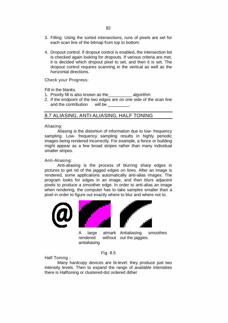
82

3. Filling: Using the sorted intersections, runs of pixels are set foreach scan line of the bitmap from top to bottom.

4. Dropout control: If dropout control is enabled, the intersection listis checked again looking for dropouts. If various criteria are met,it is decided which dropout pixel to set, and then it is set. Thedropout control requires scanning in the vertical as well as thehorizontal directions.


Fill in the blanks.1. Priority fill is also known as the__________ algorithm2. If the endpoint of the two edges are on one side of the scan line

and the contribution will be _________.

8.7 ALIASING, ANTI-ALIASING, HALF TONING

Aliasing:Aliasing is the distortion of information due to low- frequency

sampling. Low- frequency sampling results in highly periodicimages being rendered incorrectly. For example, a fence or buildingmight appear as a few broad stripes rather than many individualsmaller stripes.

Anti-Aliasing:Anti-aliasing is the process of blurring sharp edges in

pictures to get rid of the jagged edges on lines. After an image isrendered, some applications automatically anti-alias images. Theprogram looks for edges in an image, and then blurs adjacentpixels to produce a smoother edge. In order to anti-alias an imagewhen rendering, the computer has to take samples smaller than apixel in order to figure out exactly where to blur and where not to.

A large atmarkrendered withoutantialiasing

Antialiasing smoothesout the jaggies.

Fig. 8.5Half Toning :

Many hardcopy devices are bi-level: they produce just twointensity levels. Then to expand the range of available intensitiesthere is Halftoning or clustered-dot ordered dither

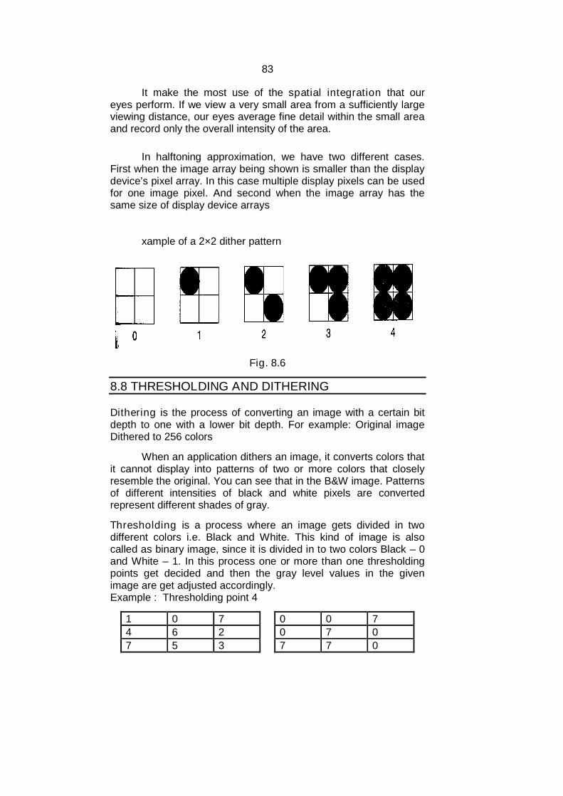
83

It make the most use of the spatial integration that oureyes perform. If we view a very small area from a sufficiently largeviewing distance, our eyes average fine detail within the small areaand record only the overall intensity of the area.

In halftoning approximation, we have two different cases.First when the image array being shown is smaller than the displaydevice’s pixel array. In this case multiple display pixels can be usedfor one image pixel. And second when the image array has thesame size of display device arrays

xample of a 2×2 dither pattern

Fig. 8.6

8.8 THRESHOLDING AND DITHERING

Dithering is the process of converting an image with a certain bitdepth to one with a lower bit depth. For example: Original imageDithered to 256 colors

When an application dithers an image, it converts colors thatit cannot display into patterns of two or more colors that closelyresemble the original. You can see that in the B&W image. Patternsof different intensities of black and white pixels are convertedrepresent different shades of gray.

Thresholding is a process where an image gets divided in twodifferent colors i.e. Black and White. This kind of image is alsocalled as binary image, since it is divided in to two colors Black – 0and White – 1. In this process one or more than one thresholdingpoints get decided and then the gray level values in the givenimage are get adjusted accordingly.Example : Thresholding point 4

1 0 7 0 0 7

4 6 2 0 7 0

7 5 3 7 7 0

84

The Original Image

3x3 image . 3bit image. L= 2bit

size =23 = 8Gray values L= 0 to 7Lmin (Black) - 0Lmax (White) - 7

Threhold Image

If color(Gray Value) <=T ---- 0 (Lmin)ElseIf color(Gray Value) >T ---- 7(Lmax)

Check your Progress:1. Define: Thresholding.2. What is anti- alising?3. Explain Half Toning.

8.9 LET US SUM UP

The pixels which are inside the polygon can be determined byusing the following two test: Inside outside test and Windingnumber test.

The scan line filling algorithm can be applied for the curveclosed boundary

Priority fill is also known as the Painter's algorithm

Anti-aliasing is the process of blurring sharp edges in pictures toget rid of the jagged edges on lines

Dithering is the process of converting an image with a certain bitdepth to one with a lower bit depth.

Thresholding is a process where an image gets divided in twodifferent colors


Procedural elements of Computer Graphics, David F. Rogers,Tata McGraw Hill.

85

Computer Graphics, ISRD Group, Tata McGraw Hill.

Computer Graphics, Amarendra Sinha, A. Udai,, Tata McGrawHill.

Computer Graphics,A. P. Godase, Technical Publications Pune.

Computer Graphics, Donald Hearn, M P. Baker, PHI.

8.11 EXERCISE

1. What are the polygon filling techniques? Explain any one.2. Write a short note on Scan conversion of character.3. Explain Inside- Outside test.4. Define: Aliasing, Anti- Aliasing.5. Write a short note on Thresholding and Dithering.

86

9

INTRODUCTION TO CURVES

Unit Structure:

9.0 Objective

9.1 Introduction

9.2 Curve Continuity

9.3 Conic Curves

9.4 Piecewise Curve Design

9.5 Parametric Curve Design

9.6 Spline Curve Representation

9.7 Bezier Curves

9.8 B-Spline Curves

9.9 Difference between Bezier Curves and B-Spline Curves

9.10 Fractals and its applications.

9.11 Let us sum up


9.13 Exercise

9.0 OBJECTIVE

The objective of this chapter is To understand concept of curve and different types of curves. To understand difference between Bezier and B- Spline curves. To understand concept of fractals and its branches and different

application areas.

9.1 INTRODUCTION

Curves (and surfaces) are specified by the user in terms ofpoints and are constructed in an interactive process. Here, are fewpoints which we have to consider since we are going to learn aboutcurves: Control Points, Multi valued, Axis Independent, Global orLocal Curve Control, Diminishing variation and versatility, Order ofcontinuity, Parametric function, Blending functions.

87

Fractal was coined in 1975, by mathematician BenoitMandelbrot to describe an intricate looking set of curves, many ofwhich were never seen before the advent of computers, because ofits ability to perform quickly massive calculations. Fractals arefigures with an infinite amount of detail. When magnified, they don’tbecome more simple, but remain as complex as they were withoutmagnification

9.2 CURVE CONTINUITY

A breakpoint is where two curve segments meet within apiecewise curve. The continuity of a curve at a breakpointdescribes how those curves meet at the breakpoint.

There are four possible types of continuity:

No continuity: It means the curves do not meet at all.

C0continuity : Here, it may be a sharp point where they meet.

C1continuity: The curves have identical tangents at the breakpointand the curves join smoothly. C2continuity: The curves haveidentical curvature at the breakpoint and curvature continuityimplies both tangential and positional continuity.

Fig. 9.1 Fig. 9.2 Fig. 9.3

9.3 CONIC CURVES

Both circles and ellipses are special cases of a class ofcurves known as conics. Conics are distinguished by second-degree discriminating functions of the form:

2 2,f x y Ax Bxy Cy Dx Ey F

The values of the constants, A, B, C, D, E, and F determinesthe type of curve as follows:

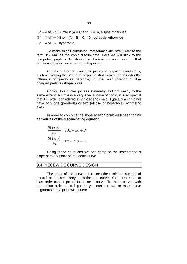
88

2 4 0B AC circle if (A = C and B = 0), ellipse otherwise2 4 0B AC line if (A = B = C = 0), parabola otherwise2 4 0B AC hyperbola

To make things confusing, mathematicians often refer to theterm B2 - 4AC as the conic discriminate. Here we will stick to thecomputer graphics definition of a discriminant as a function thatpartitions interior and exterior half-spaces.

Curves of this form arise frequently in physical simulations,such as plotting the path of a projectile shot from a canon under theinfluence of gravity (a parabola), or the near collision of like-charged particles (hyperbolas).

Conics, like circles posses symmetry, but not nearly to thesame extent. A circle is a very special case of conic, it is so specialthat it is often considered a non-generic conic. Typically a conic willhave only one (parabola) or two (ellipse or hyperbola) symmetricaxes.

In order to compute the slope at each point we'll need to findderivatives of the discriminating equation:

,2

,2

f x yAx By D

x

f x yBx Cy E

x

Using these equations we can compute the instantaneousslope at every point on the conic curve.

9.4 PIECEWISE CURVE DESIGN

The order of the curve determines the minimum number ofcontrol points necessary to define the curve. You must have atleast order control points to define a curve. To make curves withmore than order control points, you can join two or more curvesegments into a piecewise curve

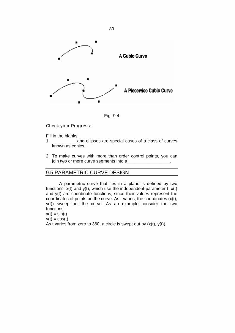
89

Fig. 9.4


Fill in the blanks.1. __________ and ellipses are special cases of a class of curves

known as conics .

2. To make curves with more than order control points, you canjoin two or more curve segments into a _________________.

9.5 PARAMETRIC CURVE DESIGN

A parametric curve that lies in a plane is defined by twofunctions, x(t) and y(t), which use the independent parameter t. x(t)and y(t) are coordinate functions, since their values represent thecoordinates of points on the curve. As t varies, the coordinates (x(t),y(t)) sweep out the curve. As an example consider the twofunctions:x(t) = sin(t)y(t) = cos(t)As t varies from zero to 360, a circle is swept out by (x(t), y(t)).

90

Fig. 9.5 Fig. 9.6

9.6 SPLINE CURVE REPRESENTATION

A spline curve is a mathematical representation for which itis easy to build an interface that will allow a user to design andcontrol the shape of complex curves and surfaces. The generalapproach is that the user enters a sequence of points, and a curveis constructed whose shape closely follows this sequence. Thepoints are called control points. A curve that actually passesthrough each control point is called an interpolating curve; a curvethat passes near to the control points but not necessarily throughthem is called an approximating curve.

Fig. 9.7

91

9.7 BEZIER CURVES

Bezier curveBezier curve section can be fitted to any number of control

points. The number of control points to be approximated and theirrelative position determine the degree of the Bezier polynomial. ABezier curve can be specified with boundary conditions, withblending function. Suppose we are given n+1 control pointpositions: Pk =(Xk,Yk,Zk) with k varing from 0 to n. thesecoordinate points can be blended to produce the following positionvector P(u) , which describes the path of an approximating Bezierpolynomial function between P0 and Pn.P(u)= ∑n

k=0 Pk BEZk ,n(u) ……….. 0≤u≤1.

The Bernstein polynomials:BEZk ,n(u) =C(n,k) uk (1-u)C(n,k)= binomial coefficients.C(n,k)=n!/ k! (n-k)!BEZk ,n(u) = (1-u) BEZk ,n-1(u) +u BEZk-1 ,n-1(u) ……….. n› k≥ 1

X(u)= ∑nk=0 Xk BEZk ,n(u)

Y(u)= ∑nk=0 Yk BEZk ,n(u)

3 points : Generate a parabola4 points : A cubic curve3 collinear controlpoints :

Generate a straight line segment

Why use?

1. Easy to implement2. Reasonably powerful in curve design.3. Efficient methods for determining coordinate positions along a

Bezier curve can be set up using recursive calculations.C(n,k)=((n-k+1)/k ) C (n,k-1) ………… n≥k.

Properties:

1. Bezier curves are always passes through the first and lastcontrol points.

2. The slop at the beginning of the curve is along the line joiningthe first two control points and the slop at the end of the curve isalong the line joining the last two end points.

3. It lies within the convex hull of the control points.

Cubic Bezier Curves.

It gives reasonable design flexibility while avoiding theincreased calculations needed with higher order polynomials.

92

BEZ0 ,3(u) = (1-u)3

BEZ1,3(u) = 3u(1-u)2

BEZ2,3(u) = 3u2(1-u)BEZ3,3(u) = u3

At u=0 and u=1 only non zero blending function is BEZ0,3

and BEZ3,3 respectively. Thus, the cubic curve will always passthrough control points P0 and P3

The BEZ1,3 and BEZ2,3 influence the shape of the curve atintermediate values of parameter u, so that the resulting curvetends toward points p1 and p2. BEZ1,3 is max at u=1/3BEZ2,3 is max at u=2/3.

Bezier curves do not allow for local control of the curveshape. If we reposition any one of the control points, the entirecurve will be affected.

9.8 B-SPLINE CURVES

B-splines are not used very often in 2D graphics softwarebut are used quite extensively in 3D modeling software. They havean advantage over Bezier curves in that they are smoother andeasier to control. B-splines consist entirely of smooth curves, butsharp corners can be introduced by joining two spline curvesegments. The continuous curve of a b-spline is defined by controlpoints.

The equation for k-order B-spline with n+1 control

points 0 1, , ... nP P P is , 1 10, ,i k i k niP t n N t P t t t .

In a B-spline each control point is associated with a basisfunction Ni,k which is given by the recurrence relations B-splinebasis functions as like as Bezier ones arenonnegative 0ikN and have "partition of unity"

property 0, 1, 1, 1n N t t t ti ni k k therefore ,0 1i kN

As since 0ikN for jt t or j kt t therefore a control

point Pi influences the curve only for ti < t < ti+k.

The main properties of B-splines composed of (n-k+2) Bezier curves of k-order joined Ck-

2 continuously at knot values (t0 , t1 , ... , tn+k) each point affected by k control points each control point affected k segments inside convex hull affine invarianc

93

uniform B-splines don't interpolate deBoor controlpoints (P0 , P1 , ... , Pn )

Check your Progress:True or False.1. Bezier curve is easy to implement.2. The continuous curve of a b-spline is defined by control points.

9.9 DIFFERENCE BETWEEN BEZIER CURVES AND B-SPLINE CURVES

Bezier Curve B-Spline Curve

Bezier curves do not need knots To construct B-splines oneneeds to specify knots

Bezier curve automaticallyclams its endpoints.

B-Splines do not interpolate anyof its control points.

Bezier curve basis functions areeasier to compute.

B-Spline curve requires morecomputations

Table 9.1

9.10 FRACTALS AND ITS APPLICATIONS

Introduction:

Fractal Geometry has found its applications not onlyanimations or film industries, creating beautiful natural objects , butalso in Biological study, Medicines, Telecommunications, FluidMechanics, Image Compression, Fractal Music etc.

“Art is the creation of mind, an idea. A painting, a piece ofmusic or a sculpture is only the embodiment of that idea. The ideathat nature and mathematics are inextricably linked can be verywell proved by using fractal geometry in Computer Graphics.Natural objects can be realistically described by fractal geometrymethods.

Fractals can be seen as mysterious expressions of beautyrepresenting exquisite preordained shapes that mimic the universe.Art and science will eventually be seen to be as closely connectedas arms to the body. Both are vital elements of order and itsdiscovery. But when art is seen as the ability to do, make, apply, orportray in way that withstands the test of time, its connection withscience becomes clearer.

94

Applications of Fractal Geometry:

Nature:Fractals have become immensely popular for describing and

creatin natural objects like mountains, clouds, flames, etc. thatcannot be described in terms of mathematical geometry usingtriangles or squares. In Computer Graphics, modeling techniquesgenerally assume that an object is a collection of lines or polygonsor that it can be described by higher order polynomials e.g. Bezieror B-Spline curves. While these techniques efficiently model solidobjects like cars, roads, houses etc. they are not well adapted torepresentation of natural object features like terrains, snow, smoke,etc.

Fig.9.8 The Fractal Fern

The Fractal FernThe "fractal fern" is generatedcompletely by fractals. This isnot a digital photograph - it iscompletely computer-generated.

Animations & movies:The application of fractal has mostly been in the field of

animations, motion pictures and visualizations. E.g.: Real popularapplication is in form of Imaginary Landscapes of outer space inSTAR TREK, STAR WARS. Here UCLA mathematicians along withHollywood filmmakers used the 3D fractals beautifully and createdlandscapes which looked very real; but were non-existent. Fractalimages are used as an alternative to costly elaborate sets toproduce fantasy landscapes.

Bacteria Cultures:Some of the most amazing applications of fractals can be

found in such distant areas as the shapes of bacteria cultures. Abacteria culture is all bacteria that originated from a single ancestorand are living in the same place. When a culture is growing, itspreads outwards in different directions from the place where theoriginal organism was placed. Just like plants the spreadingbacteria can branch and form patterns which turn out to be fractal.The spreading of bacteria can be modeled by fractals such as thediffusion fractals, because bacteria spread similarly to nonlivingmaterials.

95

Biological systems:Fractal and chaos phenomena specific to non-linear systems

are widely observed in biological systems. A study has beenestablished an analytical method based on fractals and chaostheory for two patterns: the dendrite pattern of cells duringdevelopment in the cerebellum and the firing pattern of intercellularpotential. Variation in the development of the dendrite stage wasevaluated with fractal dimension, enabling the high order seenthere to be quantized

Origin of Fractals:

With the aid of computer graphics, Mandelbrot who thenworked at IBM's Watson Research Center was able to show howJulia's work is a source of some of the most beautiful fractalsknown today. By iterating a simple equation and mapping thisequation in the complex plane, Mandelbrot discovered the fractalnamed after his name, Mandelbrot Set. He has been initiallyresponsible for extending the theory and graphics representation ofiterated functions as a special class of new geometry as “FractalGeometry”.

The fact that any small part of the coast will look similar tothe whole thing was first noted by Benoit Mandelbrot. He calledshapes like this fractals. In nature, you can find them everywhere.Any tree branch, when magnified, looks like the entire tree. Anyrock from a mountain looks like the entire mountain. The theory offractals was first developed to study nature. Now it is used in avariety of other applications. And, of course, beauty is what makesthem popular! And now fractal geometry is providing us with a newperspective to view the world, creating real life landscapes, to datacompression, music etc.

Advantages of using Fractal Geometry:

Fractal was coined in 1975, by mathematician BenoitMandelbrot to describe an intricate looking set of curves, many ofwhich were never seen before the advent of computers, because ofits ability to perform quickly massive calculations.

Fractals are figures with an infinite amount of detail. Whenmagnified, they don’t become more simple, but remain as complexas they were without magnification.

The modeling and rendering time required is minimalcompared with traditional methods. In this respect our newapproach is comparable to the old one, though it’s slower for large,complex scenes.

96

L-system can be considered as a compression of the film with afactor typically bigger than one million. In general, a productionsystem needs not to build up a 3D database to the completeenvironment. It can directly draw objects during the interpretation ofa symbolic environment string.

In the case of fractals, few properties are: a fine structure, too much irregularity to be described in traditional geometric

language, both locally and globally, some form of self-similarity, perhaps approximate or statistical, a "fractal dimension"(somehow defined) which is greater than its

topological dimension, and A simple definition, perhaps recursive.

Classification of IFS and complex fractals:

Fig. 9.9

The term “fractal” was introduced for characterizing spatial ortemporal phenomena that are continuous but not differentiable(Mandelbrot, 1975).

Fractal is defined as a rough or fragmented geometric shapethat can be sub-divided into parts, each of which is (at leastapproximately) a reduced size copy of the whole. Mathematically, afractal is defined as a set of points whose fractal dimensionexceeds its topological dimension (Mandelbrot, 1983).

In general, the dimension of a fractal is typically a non-integer or a fraction, meaning its dimension is not a whole numberand its formation is by an iteration (or recursive) process, and

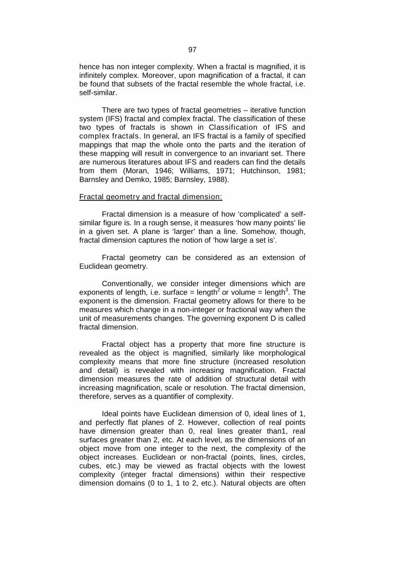
97

hence has non integer complexity. When a fractal is magnified, it isinfinitely complex. Moreover, upon magnification of a fractal, it canbe found that subsets of the fractal resemble the whole fractal, i.e.self-similar.

There are two types of fractal geometries – iterative functionsystem (IFS) fractal and complex fractal. The classification of thesetwo types of fractals is shown in Classification of IFS andcomplex fractals. In general, an IFS fractal is a family of specifiedmappings that map the whole onto the parts and the iteration ofthese mapping will result in convergence to an invariant set. Thereare numerous literatures about IFS and readers can find the detailsfrom them (Moran, 1946; Williams, 1971; Hutchinson, 1981;Barnsley and Demko, 1985; Barnsley, 1988).

Fractal geometry and fractal dimension:

Fractal dimension is a measure of how ‘complicated’ a self-similar figure is. In a rough sense, it measures ‘how many points’ liein a given set. A plane is ‘larger’ than a line. Somehow, though,fractal dimension captures the notion of ‘how large a set is’.

Fractal geometry can be considered as an extension ofEuclidean geometry.

Conventionally, we consider integer dimensions which areexponents of length, i.e. surface = length2 or volume = length3. Theexponent is the dimension. Fractal geometry allows for there to bemeasures which change in a non-integer or fractional way when theunit of measurements changes. The governing exponent D is calledfractal dimension.

Fractal object has a property that more fine structure isrevealed as the object is magnified, similarly like morphologicalcomplexity means that more fine structure (increased resolutionand detail) is revealed with increasing magnification. Fractaldimension measures the rate of addition of structural detail withincreasing magnification, scale or resolution. The fractal dimension,therefore, serves as a quantifier of complexity.

Ideal points have Euclidean dimension of 0, ideal lines of 1,and perfectly flat planes of 2. However, collection of real pointshave dimension greater than 0, real lines greater than1, realsurfaces greater than 2, etc. At each level, as the dimensions of anobject move from one integer to the next, the complexity of theobject increases. Euclidean or non-fractal (points, lines, circles,cubes, etc.) may be viewed as fractal objects with the lowestcomplexity (integer fractal dimensions) within their respectivedimension domains (0 to 1, 1 to 2, etc.). Natural objects are often

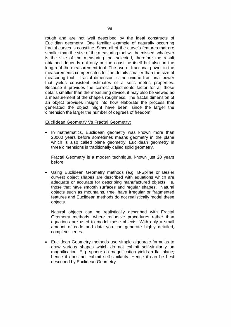
98

rough and are not well described by the ideal constructs ofEuclidian geometry .One familiar example of naturally occurringfractal curves is coastline. Since all of the curve’s features that aresmaller than the size of the measuring tool will be missed, whateveris the size of the measuring tool selected, therefore the resultobtained depends not only on the coastline itself but also on thelength of the measurement tool. The use of fractional power in themeasurements compensates for the details smaller than the size ofmeasuring tool – fractal dimension is the unique fractional powerthat yields consistent estimates of a set’s metric properties.Because it provides the correct adjustments factor for all thosedetails smaller than the measuring device, it may also be viewed asa measurement of the shape’s roughness. The fractal dimension ofan object provides insight into how elaborate the process thatgenerated the object might have been, since the larger thedimension the larger the number of degrees of freedom.

Euclidean Geometry Vs Fractal Geometry:

In mathematics, Euclidean geometry was known more than20000 years before sometimes means geometry in the planewhich is also called plane geometry. Euclidean geometry inthree dimensions is traditionally called solid geometry.

Fractal Geometry is a modern technique, known just 20 yearsbefore.

Using Euclidean Geometry methods (e.g. B-Spline or Beziercurves) object shapes are described with equations which areadequate or accurate for describing manufactured objects, i.e.those that have smooth surfaces and regular shapes. Naturalobjects such as mountains, tree, have irregular or fragmentedfeatures and Euclidean methods do not realistically model theseobjects.

Natural objects can be realistically described with FractalGeometry methods, where recursive procedures rather thanequations are used to model these objects. With only a smallamount of code and data you can generate highly detailed,complex scenes.

Euclidean Geometry methods use simple algebraic formulas todraw various shapes which do not exhibit self-similarity onmagnification. E.g. sphere on magnification yields a flat plane;hence it does not exhibit self-similarity. Hence it can be bestdescribed by Euclidean Geometry.

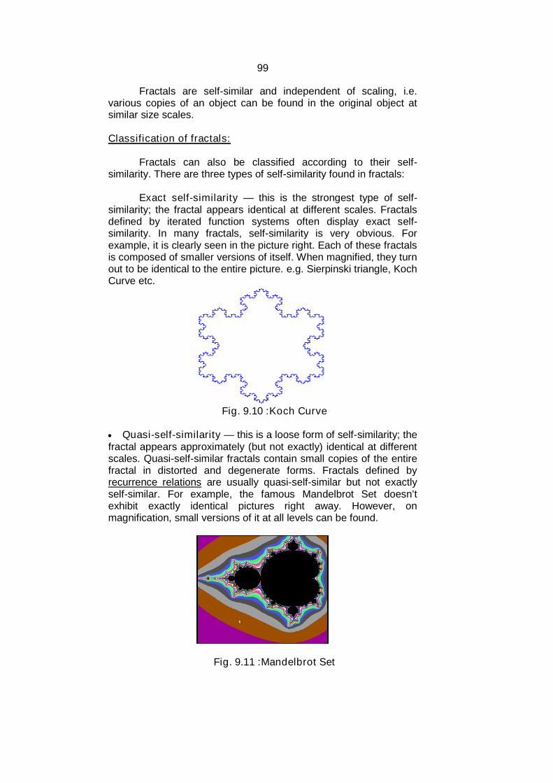
99

Fractals are self-similar and independent of scaling, i.e.various copies of an object can be found in the original object atsimilar size scales.

Classification of fractals:

Fractals can also be classified according to their self-similarity. There are three types of self-similarity found in fractals:

Exact self-similarity — this is the strongest type of self-similarity; the fractal appears identical at different scales. Fractalsdefined by iterated function systems often display exact self-similarity. In many fractals, self-similarity is very obvious. Forexample, it is clearly seen in the picture right. Each of these fractalsis composed of smaller versions of itself. When magnified, they turnout to be identical to the entire picture. e.g. Sierpinski triangle, KochCurve etc.

Fig. 9.10 :Koch Curve

Quasi-self-similarity — this is a loose form of self-similarity; thefractal appears approximately (but not exactly) identical at differentscales. Quasi-self-similar fractals contain small copies of the entirefractal in distorted and degenerate forms. Fractals defined byrecurrence relations are usually quasi-self-similar but not exactlyself-similar. For example, the famous Mandelbrot Set doesn’texhibit exactly identical pictures right away. However, onmagnification, small versions of it at all levels can be found.

Fig. 9.11 :Mandelbrot Set

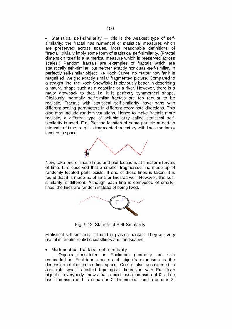
100

Statistical self-similarity — this is the weakest type of self-similarity; the fractal has numerical or statistical measures whichare preserved across scales. Most reasonable definitions of"fractal" trivially imply some form of statistical self-similarity. (Fractaldimension itself is a numerical measure which is preserved acrossscales.) Random fractals are examples of fractals which arestatistically self-similar, but neither exactly nor quasi-self-similar. Inperfectly self-similar object like Koch Curve, no matter how far it ismagnified, we get exactly similar fragmented picture. Compared toa straight line, the Koch Snowflake is obviously better in describinga natural shape such as a coastline or a river. However, there is amajor drawback to that, i.e. it is perfectly symmetrical shape.Obviously, normally self-similar fractals are too regular to berealistic. Fractals with statistical self-similarity have parts withdifferent scaling parameters in different coordinate directions. Thisalso may include random variations. Hence to make fractals morerealistic, a different type of self-similarity called statistical self-similarity is used. E.g. Plot the location of some particle at certainintervals of time; to get a fragmented trajectory with lines randomlylocated in space.

Now, take one of these lines and plot locations at smaller intervalsof time. It is observed that a smaller fragmented line made up ofrandomly located parts exists. If one of these lines is taken, it isfound that it is made up of smaller lines as well. However, this self-similarity is different. Although each line is composed of smallerlines, the lines are random instead of being fixed.

Fig. 9.12 :Statistical Self-Similarity

Statistical self-similarity is found in plasma fractals. They are veryuseful in creatin realistic coastlines and landscapes.

Mathematical fractals - self-similarityObjects considered in Euclidean geometry are sets

embedded in Euclidean space and object’s dimension is thedimension of the embedding space. One is also accustomed toassociate what is called topological dimension with Euclideanobjects - everybody knows that a point has dimension of 0, a linehas dimension of 1, a square is 2 dimensional, and a cube is 3-

101

dimensional. The topological dimension is preserved when theobjects are transformed by a homeomorphism. One cannot usetopological dimension for fractals, but instead has to use what iscalled Hausdorff-Besikovitch dimension, commonly known asfractal dimension. In fact, a formal definition of a fractal says that itis an object for which the fractal dimension is greater than thetopological dimension. But this definition is too restrictive. Analternative definition uses the concept of self-similarity – a fractal isan object made of parts similar to the whole. The notion of self-similarity is the basic property of fractal objects. Taking advantageof self-similarity is one way (called similarity method) to calculatefractal dimension.

For example, one can subdivide a line segment into m self-similar intervals, each with the same length, and each of which canbe magnified by a factor of n to yield the original segment. A squareor a triangle may be subdivided into n2 self-similar copies of itself,each of which must be magnified by a factor of n to yield theoriginal object. Similarly, a cube can be decomposed into n2 self-similar copies of itself, each of which must be magnified by a factorof n to yield the original cube (Table 1). If one takes themagnification, n , and raise it to the power of dimension, D , one willget the number of self-similar pieces in the original object, P: P = nD

Solving this equation for D one easily finds thatD = log(P) / log(n)Using this formula one can calculate fractal dimension of

some fractals.

Object Dimension No. of Copies

Line 1 2 = 21

Square 2 4 = 22

Cube 3 8 = 23

Anyself-similar figure

D P = 2D

Sierpinski triangle 1.58 3 = 2D

Table 9.2

A mathematical fractal has some infinitely repeating patternand can be made by the iteration of a certain rule.

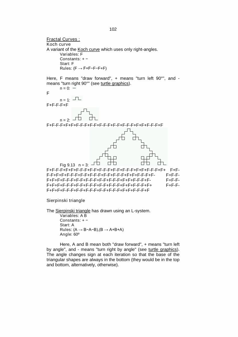
102

Fractal Curves :Koch curveA variant of the Koch curve which uses only right-angles.

Variables: FConstants: + −Start: FRules: (F → F+F−F−F+F)

Here, F means "draw forward", + means "turn left 90°", and -means "turn right 90°" (see turtle graphics).

n = 0:F

n = 1:F+F-F-F+F

n = 2:

F+F-F-F+F+F+F-F-F+F-F+F-F-F+F-F+F-F-F+F+F+F-F-F+F

Fig 9.13 n = 3:F+F-F-F+F+F+F-F-F+F-F+F-F-F+F-F+F-F-F+F+F+F-F-F+F+ F+F-F-F+F+F+F-F-F+F-F+F-F-F+F-F+F-F-F+F+F+F-F-F+F- F+F-F-F+F+F+F-F-F+F-F+F-F-F+F-F+F-F-F+F+F+F-F-F+F- F+F-F-F+F+F+F-F-F+F-F+F-F-F+F-F+F-F-F+F+F+F-F-F+F+ F+F-F-F+F+F+F-F-F+F-F+F-F-F+F-F+F-F-F+F+F+F-F-F+F

Sierpinski triangle

The Sierpinski triangle has drawn using an L-system.Variables: A BConstants: + −Start: ARules: (A → B−A−B),(B → A+B+A) Angle: 60º

Here, A and B mean both "draw forward", + means "turn leftby angle", and - means "turn right by angle" (see turtle graphics).The angle changes sign at each iteration so that the base of thetriangular shapes are always in the bottom (they would be in the topand bottom, alternatively, otherwise).

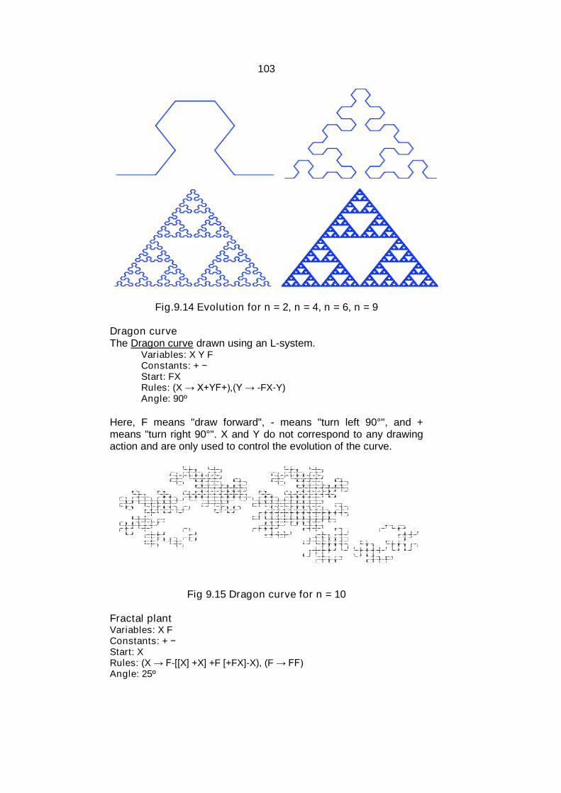
103

Fig.9.14 Evolution for n = 2, n = 4, n = 6, n = 9

Dragon curveThe Dragon curve drawn using an L-system.

Variables: X Y FConstants: + −Start: FXRules: (X → X+YF+),(Y → -FX-Y)Angle: 90º

Here, F means "draw forward", - means "turn left 90°", and +means "turn right 90°". X and Y do not correspond to any drawingaction and are only used to control the evolution of the curve.

Fig 9.15 Dragon curve for n = 10

Fractal plantVariables: X FConstants: + −Start: XRules: (X → F-[[X] +X] +F [+FX]-X), (F → FF) Angle: 25º

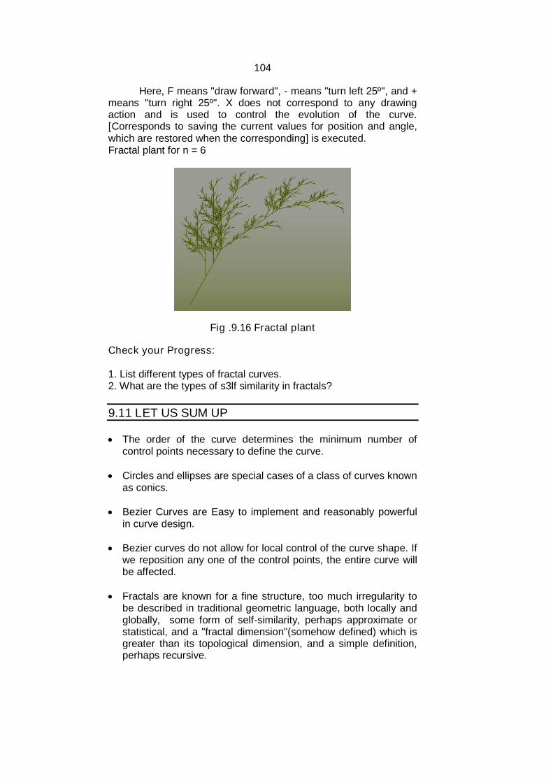
104

Here, F means "draw forward", - means "turn left 25º", and +means "turn right 25º". X does not correspond to any drawingaction and is used to control the evolution of the curve.[Corresponds to saving the current values for position and angle,which are restored when the corresponding] is executed.Fractal plant for n = 6

Fig .9.16 Fractal plant


1. List different types of fractal curves.2. What are the types of s3lf similarity in fractals?

9.11 LET US SUM UP

The order of the curve determines the minimum number ofcontrol points necessary to define the curve.

Circles and ellipses are special cases of a class of curves knownas conics.

Bezier Curves are Easy to implement and reasonably powerfulin curve design.

Bezier curves do not allow for local control of the curve shape. Ifwe reposition any one of the control points, the entire curve willbe affected.

Fractals are known for a fine structure, too much irregularity tobe described in traditional geometric language, both locally andglobally, some form of self-similarity, perhaps approximate orstatistical, and a "fractal dimension"(somehow defined) which isgreater than its topological dimension, and a simple definition,perhaps recursive.

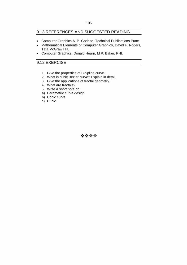
105


Computer Graphics,A. P. Godase, Technical Publications Pune. Mathematical Elements of Computer Graphics, David F. Rogers,

Tata McGraw Hill. Computer Graphics, Donald Hearn, M P. Baker, PHI.

9.12 EXERCISE

1. Give the properties of B-Spline curve.2. What is cubic Bezier curve? Explain in detail.3. Give the applications of fractal geometry.4. What are fractals?5. Write a short note on:a) Parametric curve designb) Conic curvec) Cubic

106

10

SURFACE DESIGN AND VISIBLESURFACES

Unit Structure:

10.0 Objectives

10.1 Introduction

10.2 Types of surfaces

10.2.1 Bilinear Surfaces

10.2.2 Ruled Surfaces

10.2.3 Developable Surfaces

10.2.4 Coons Patch

10.2.5 Sweep Surfaces

10.2.6 Surface of Revolution

10.2.7 Quadric Surfaces

10.3 Constructive Solid Geometry

10.3.1 Bezier Surfaces

10.3.2 BSpline Surfaces

10.3.3 Subdivision Surfaces

10.4 Introduction to visible and hidden surfaces

10.5 Coherence for visibility

10.6 Extents and Bounding Volumes

10.7 Back FaceCulling

10.8 Painter’s Algorithm

10.9 Z-Buffer Algorithm

10.10 Floating Horizon Algorithm

10.11 Roberts Algorithm

10.12 Let us sum up


10.14 Exercise

10.0 OBJECTIVE

The objective of this chapter is To understand the different types of surfaces. To understand concept of solid geometry.

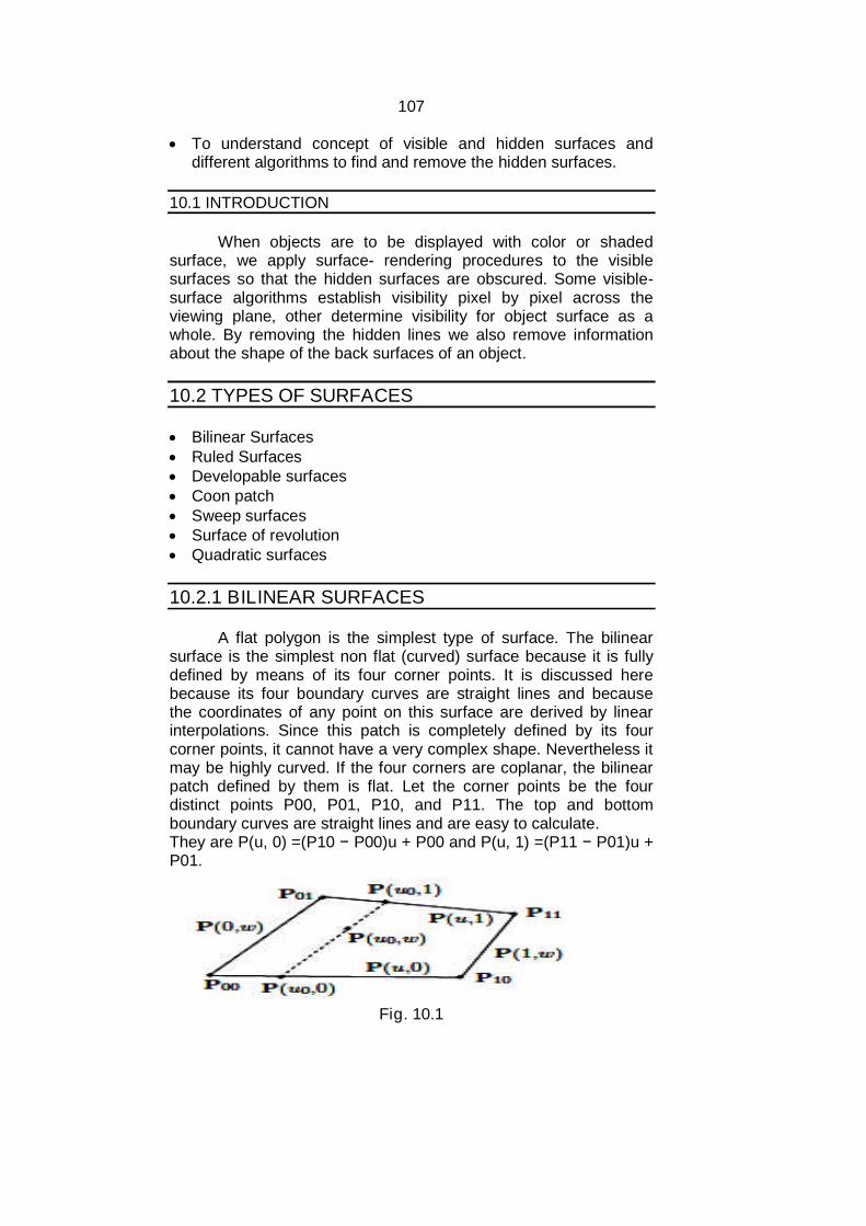
107

To understand concept of visible and hidden surfaces anddifferent algorithms to find and remove the hidden surfaces.

10.1 INTRODUCTION

When objects are to be displayed with color or shadedsurface, we apply surface- rendering procedures to the visiblesurfaces so that the hidden surfaces are obscured. Some visible-surface algorithms establish visibility pixel by pixel across theviewing plane, other determine visibility for object surface as awhole. By removing the hidden lines we also remove informationabout the shape of the back surfaces of an object.

10.2 TYPES OF SURFACES

Bilinear Surfaces Ruled Surfaces Developable surfaces Coon patch Sweep surfaces Surface of revolution Quadratic surfaces

10.2.1 BILINEAR SURFACES

A flat polygon is the simplest type of surface. The bilinearsurface is the simplest non flat (curved) surface because it is fullydefined by means of its four corner points. It is discussed herebecause its four boundary curves are straight lines and becausethe coordinates of any point on this surface are derived by linearinterpolations. Since this patch is completely defined by its fourcorner points, it cannot have a very complex shape. Nevertheless itmay be highly curved. If the four corners are coplanar, the bilinearpatch defined by them is flat. Let the corner points be the fourdistinct points P00, P01, P10, and P11. The top and bottomboundary curves are straight lines and are easy to calculate.They are P(u, 0) =(P10 − P00)u + P00 and P(u, 1) =(P11 − P01)u +P01.

Fig. 10.1

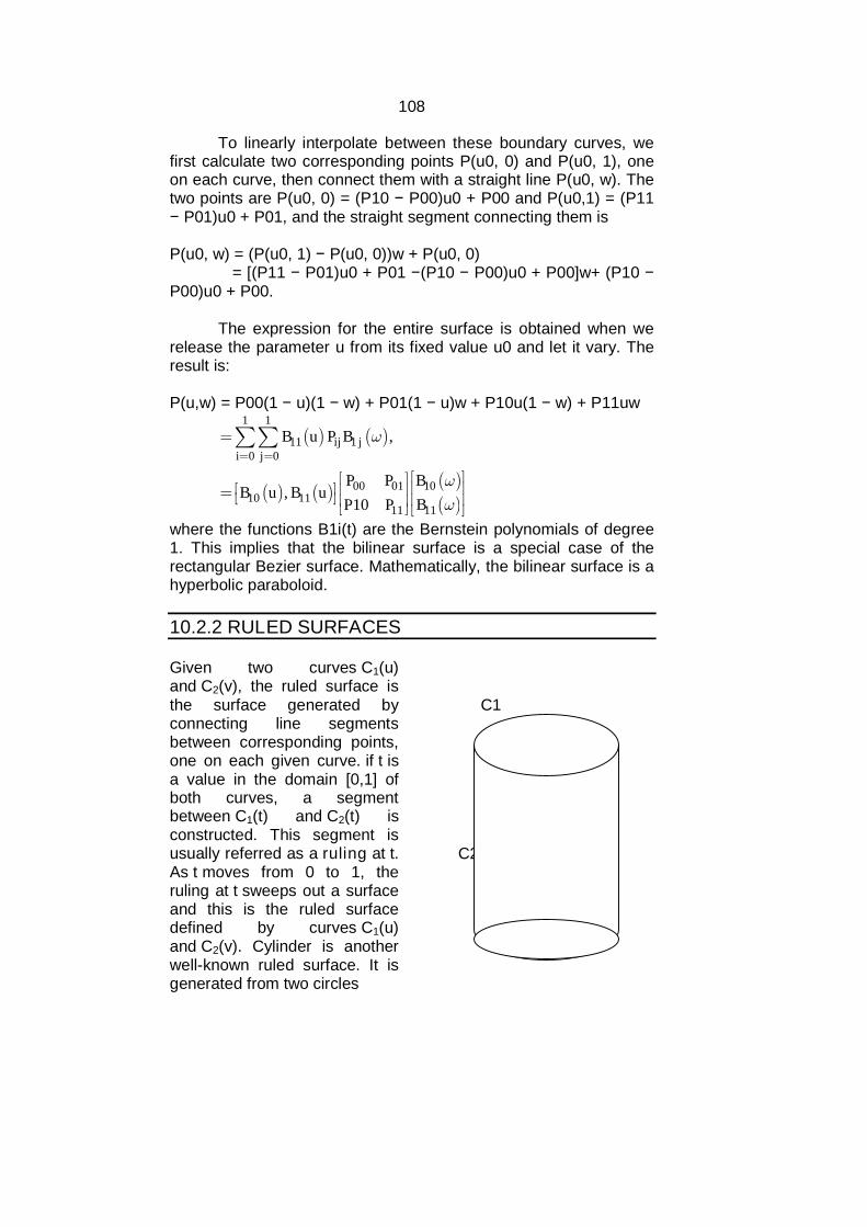
108

To linearly interpolate between these boundary curves, wefirst calculate two corresponding points P(u0, 0) and P(u0, 1), oneon each curve, then connect them with a straight line P(u0, w). Thetwo points are P(u0, 0) = (P10 − P00)u0 + P00 and P(u0,1) = (P11− P01)u0 + P01, and the straight segment connecting them is

P(u0, w) = (P(u0, 1) − P(u0, 0))w + P(u0, 0)= [(P11 − P01)u0 + P01 −(P10 − P00)u0 + P00]w+ (P10 −

P00)u0 + P00.

The expression for the entire surface is obtained when werelease the parameter u from its fixed value u0 and let it vary. Theresult is:

P(u,w) = P00(1 − u)(1 − w) + P01(1 − u)w + P10u(1 − w) + P11uw

1 1

11 10 0

1000 0110 11

1111

,

,10

ij ji j

B u P B

BP PB u B u

BP P

where the functions B1i(t) are the Bernstein polynomials of degree1. This implies that the bilinear surface is a special case of therectangular Bezier surface. Mathematically, the bilinear surface is ahyperbolic paraboloid.

10.2.2 RULED SURFACES

Given two curves C1(u)and C2(v), the ruled surface isthe surface generated byconnecting line segmentsbetween corresponding points,one on each given curve. if t isa value in the domain [0,1] ofboth curves, a segmentbetween C1(t) and C2(t) isconstructed. This segment isusually referred as a ruling at t.As t moves from 0 to 1, theruling at t sweeps out a surfaceand this is the ruled surfacedefined by curves C1(u)and C2(v). Cylinder is anotherwell-known ruled surface. It isgenerated from two circles

C1

C2

Fig. 10.2

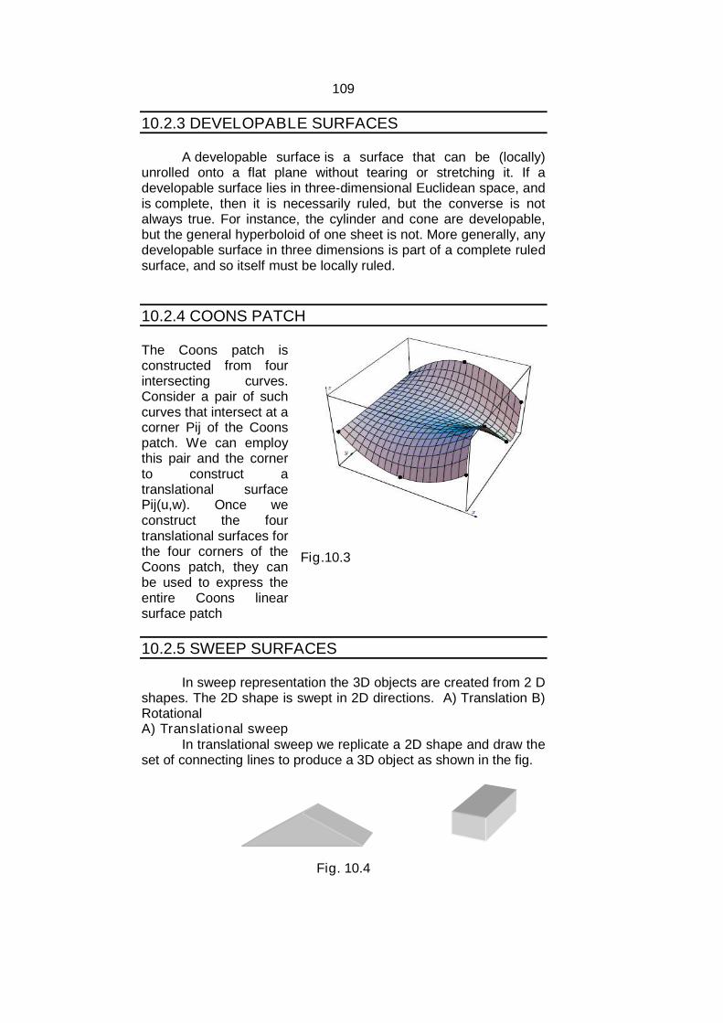
109

10.2.3 DEVELOPABLE SURFACES

A developable surface is a surface that can be (locally)unrolled onto a flat plane without tearing or stretching it. If adevelopable surface lies in three-dimensional Euclidean space, andis complete, then it is necessarily ruled, but the converse is notalways true. For instance, the cylinder and cone are developable,but the general hyperboloid of one sheet is not. More generally, anydevelopable surface in three dimensions is part of a complete ruledsurface, and so itself must be locally ruled.

10.2.4 COONS PATCH

The Coons patch isconstructed from fourintersecting curves.Consider a pair of suchcurves that intersect at acorner Pij of the Coonspatch. We can employthis pair and the cornerto construct atranslational surfacePij(u,w). Once weconstruct the fourtranslational surfaces forthe four corners of theCoons patch, they canbe used to express theentire Coons linearsurface patch

Fig.10.3

10.2.5 SWEEP SURFACES

In sweep representation the 3D objects are created from 2 Dshapes. The 2D shape is swept in 2D directions. A) Translation B)RotationalA) Translational sweep

In translational sweep we replicate a 2D shape and draw theset of connecting lines to produce a 3D object as shown in the fig.

Fig. 10.4

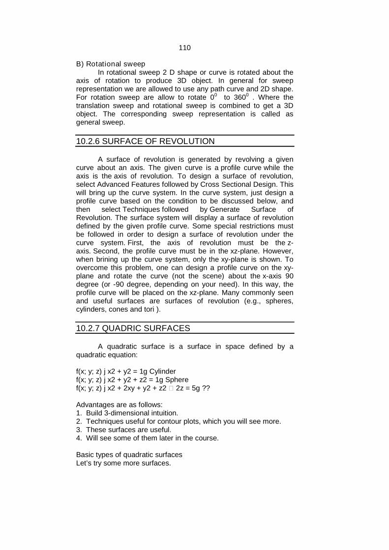
110

B) Rotational sweepIn rotational sweep 2 D shape or curve is rotated about the

axis of rotation to produce 3D object. In general for sweeprepresentation we are allowed to use any path curve and 2D shape.For rotation sweep are allow to rotate 00 to 3600 . Where thetranslation sweep and rotational sweep is combined to get a 3Dobject. The corresponding sweep representation is called asgeneral sweep.

10.2.6 SURFACE OF REVOLUTION

A surface of revolution is generated by revolving a givencurve about an axis. The given curve is a profile curve while theaxis is the axis of revolution. To design a surface of revolution,select Advanced Features followed by Cross Sectional Design. Thiswill bring up the curve system. In the curve system, just design aprofile curve based on the condition to be discussed below, andthen select Techniques followed by Generate Surface ofRevolution. The surface system will display a surface of revolutiondefined by the given profile curve. Some special restrictions mustbe followed in order to design a surface of revolution under thecurve system. First, the axis of revolution must be the z-axis. Second, the profile curve must be in the xz-plane. However,when brining up the curve system, only the xy-plane is shown. Toovercome this problem, one can design a profile curve on the xy-plane and rotate the curve (not the scene) about the x-axis 90degree (or -90 degree, depending on your need). In this way, theprofile curve will be placed on the xz-plane. Many commonly seenand useful surfaces are surfaces of revolution (e.g., spheres,cylinders, cones and tori ).

10.2.7 QUADRIC SURFACES

A quadratic surface is a surface in space defined by aquadratic equation:

f(x; y; z) j x2 + y2 = 1g Cylinderf(x; y; z) j x2 + y2 + z2 = 1g Spheref(x; y; z) j x2 + 2xy + y2 + z2 � 2z = 5g ??

Advantages are as follows:1. Build 3-dimensional intuition.2. Techniques useful for contour plots, which you will see more.3. These surfaces are useful.4. Will see some of them later in the course.

Basic types of quadratic surfacesLet’s try some more surfaces.

111

1. f(x; y; z) j x2 + y2/2 + z2/3 = 1 g: An ellipsoid2. f(x; y; z) j x2 + y2 - z2 = 1 g: A hyperboloid of one sheet3. f(x; y; z) j x2 + y2 - z2 = -1 g: A hyperboloid of two sheets4. f(x; y; z) j x2 + y2 - z2 = 0 g: A cone5. f(x; y; z) j z = x2 + y2 g: An (elliptic) paraboloid6. f(x; y; z) j z = x2 - y2 g: A hyperbolic paraboloid


1. What do you mean by developable surface?2. Define: Translational Sweep and Rotational Sweep.

10.3 CONSTRUCTIVE SOLID GEOMETRY

Constructive solid geometric representation

Here, we combine 3D objects using set operations such as,union, intersection and many more. Here, the 3D object is definedby a volume function and 2 or more volumes are combined togenerate a new shape or a new object.

Fig. 10.5

In CSG method we can use objects such as blocks,cylinders, pyramids, cones, spheres, splines.

Fig. 10.6

A good graphic package always provides these 3D shapesand the different operations and transformations that can beapplied.

10.3.1 BEZIER SURFACES

To create a Bezier surface, we blend a mesh of Beziercurves using the blending function

, , ,0 0

,m n

j k j m k nj k

P u v P BEZ v BEZ u

where j and k are points in

parametric space and ,x yP represents the location of the knots in

real space. The Bezier functions specify the weighting of aparticular knot. They are the Bernstein coefficients. The definition of

112

the Bezier functions is , , 1u kk

k nBEZ u C n k u u

. Where

,C n k represents the binary coefficients. When u=0, the function

is one for k=0 and zero for all other points. When we combine twoorthogonal parameters, we find a Bezier curve along each edge ofthe surface, as defined by the points along that edge. Beziersurfaces are useful for interactive design and were first applied tocar body design.

10.3.2 BSPLINE SURFACES

The equation of a B-spline surface follows directly from theequation of a B-spline curve. This relationship is analogous to thatbetween Bezier curves and surfaces. Furthermore, we define the B-spline surface, like the Bzier surface, in terms of a characteristicpolyhedron. The shape of the surface approximates thepolyhedron. The approximation is weaker the higher the degree.

The tensor product equation of the B-spline surface is

, , ,0 0

,m n

i p j q i ji j

P u v N u N v P

Where Ni,p(u) and Nj,q(v) are B-

spline basis functions of degree p and q, respectively. Note thatthe fundamental identities, one for each direction, must hold: h =m + p + 1 and k = n + q + 1. Therefore, a B-spline surface isanother example of tensor product surfaces. As in Bezier surfaces,the set of control points is usually referred to as the controlnet and the range of u and v is 0 and 1. Hence, a B-spline surfacemaps the unit square to a rectangular surface patch.

10.3.3 SUBDIVISION SURFACES

Subdivision surfaces are defined recursively. The processstarts with a given polygonal mesh. A refinement scheme is thenapplied to this mesh. This process takes that mesh and subdividesit, creating new vertices and new faces. The positions of the newvertices in the mesh are computed based on the positions ofnearby old vertices. In some refinement schemes, the positions ofold vertices might also be altered (possibly based on the positionsof new vertices).

This process produces a denser mesh than the original one,containing more polygonal faces. This resulting mesh can bepassed through the same refinement scheme again and so on.

The limit subdivision surface is the surface produced fromthis process being iteratively applied infinitely many times. Inpractical use however, this algorithm is only applied a limitednumber of times.

113


Fill in the Blanks.1. Subdivision surfaces are defined _________.2. A B-spline surface maps the unit square to a ________surface

patch.

10.4 INTRODUCTION TO VISIBLE AND HIDDENSURFACES

In graphics, a picture /scene consists of objects which arenearer to the “eye“ or block. The other objects are block, some partof the other objects.

The part which cannot be visible needs to be removed togive a realistic effect.

The problem of removing the unwanted surfaces and line iscalled “hidden surface problem”. There are two methods used tosolve hidden surface problem:

Image- Space Method Object –Space Method

Image - Space Method Here, we compare every object within the scene with pixel

location on the screen Here, we apply screen coordinates with above mention

conversion. If n is the number of objects and N is the number of pixels, then

the computational work increases proportional to the product . The method dependent on the precession of the screen

representation. The objects enlarge themselves significantly and do not give

correct results Eg. Z- Buffer Algorithms.

10.5 COHERENCE FOR VISIBILITY

Coherence is the result of local similarity which can becalculated using the results calculated for one part of the scene orimage for other nearby parts as objects have continuous spatialextent, object properties vary smoothly within a small local region inthe scene. Calculations can then be made incremental.

114

Types of coherence:

1. Object Coherence: Visibility of an object can often be decidedby examining a circumscribing solid (which may be of simpleform, eg. A sphere or a polyhedron.)

2. Face Coherence: Surface properties computed for one part of aface can be applied to adjacent parts after small incrementalmodification. (eg. If the face is small, we sometimes can assumeif one part of the face is invisible to the viewer, the entire face isalso invisible).

3. Edge Coherence: The Visibility of an edge changes only whenit crosses another edge, so if one segment of an nonintersectingedge is visible, the entire edge is also visible.

4. Scan line Coherence: Line or surface segments visible in onescan line are also likely to be visible in adjacent scan lines.Consequently, the image of a scan line is similar to the image ofadjacent scan lines.

5. Area and Span Coherence: A group of adjacent pixels in animage is often covered by the same visible object. Thiscoherence is based on the assumption that a small enoughregion of pixels will most likely lie within a single polygon. Thisreduces computation effort in searching for those polygonswhich contain a given screen area (region of pixels) as in somesubdivision algorithms.

6. Depth Coherence: The depths of adjacent parts of the samesurface are similar.

7. Frame Coherence: Pictures of the same scene at successivepoints in time are likely to be similar, despite small changes inobjects and viewpoint, except near the edges of moving objects.

Most visible surface detection methods make use of one ormore of these coherence properties of a scene. To take advantageof regularities in a scene, eg. Constant relationships often can beestablished between objects and surfaces in a scene.

10.6 EXTENTS AND BOUNDING VOLUMES

Bounding volume for a set of objects is a closed volume thatcompletely contains the union of the objects in the set. Boundingvolumes are used to improve the efficiency of geometricaloperations by using simple volumes to contain more complexobjects. Normally, simpler volumes have simpler ways to test foroverlap. A bounding volume for a set of objects is also a bounding

115

volume for the single object consisting of their union, and the otherway around. Therefore it is possible to confine the description to thecase of a single object, which is assumed to be non-empty andbounded (finite). Bounding volumes are most often used toaccelerate certain kinds of tests. In ray tracing, bounding volumesare used in ray-intersection tests, and in many renderingalgorithms, they are used for viewing frustum tests. If the ray orviewing frustum does not intersect the bounding volume, it cannotintersect the object contained in the volume. These intersectiontests produce a list of objects that must be displayed. Here,displayed means rendered or rasterized. In collision detection,when two bounding volumes do not intersect, then the containedobjects cannot collide, either.

Common types of bounding volumeA bounding sphere is a sphere containing the object. In 2-Dgraphics, this is a circle.

A bounding ellipsoid is an ellipsoid containing the object.Ellipsoids usually provide tighter fitting than a sphere.

A bounding cylinder is a cylinder containing the object.

A bounding capsule is a swept sphere (i.e. the volume that asphere takes as it moves along a straight line segment) containingthe object

A bounding box is a cuboid, or in 2-D a rectangle containing theobject


True or False.1. In ray tracing, bounding volumes are used in ray-intersection

tests.2. Coherence is the result of global similarity.

10.7 BACK FACECULLING

Back face culling is when you do not render a polygonbecause its normal is pointing away from the viewer's eye point. Anaive way of preforming this check would be to construct a vectorfrom the eye point to a point on the face and compute the dotproduct of this line of sight vector and the normal vector. If thisscalar is positive then the face is pointing away and consequentlycan be culled. A more sophisticated way of making this check is totransform the face's normal into the projection space, where the lineof sight vector is always the negative Z-axis. Then the check for

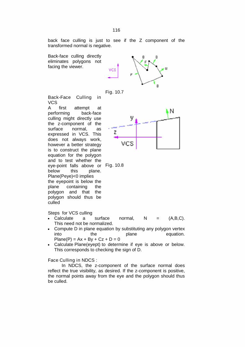
116

back face culling is just to see if the Z component of thetransformed normal is negative.

Back-face culling directlyeliminates polygons notfacing the viewer.

Fig. 10.7Back-Face Culling inVCSA first attempt atperforming back-faceculling might directly usethe z-component of thesurface normal, asexpressed in VCS. Thisdoes not always work,however a better strategyis to construct the planeequation for the polygonand to test whether theeye-point falls above orbelow this plane.Plane(Peye)<0 impliesthe eyepoint is below theplane containing thepolygon and that thepolygon should thus beculled

Fig. 10.8

Steps for VCS culling Calculate a surface normal, N = (A,B,C).

This need not be normalized. Compute D in plane equation by substituting any polygon vertex

into the plane equation.Plane(P) = Ax + By + Cz + D = 0

Calculate Plane(eyept) to determine if eye is above or below.This corresponds to checking the sign of D.

Face Culling in NDCS :In NDCS, the z-component of the surface normal does

reflect the true visibility, as desired. If the z-component is positive,the normal points away from the eye and the polygon should thusbe culled.

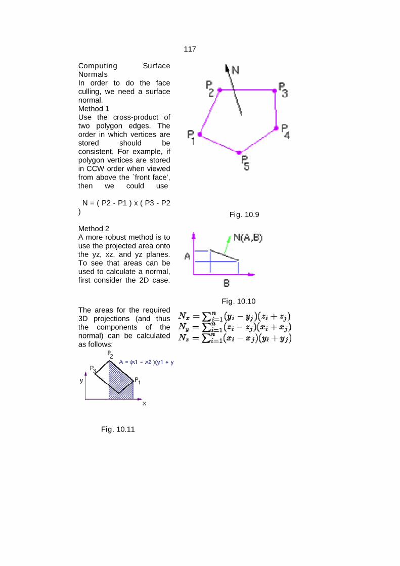
117

Computing SurfaceNormalsIn order to do the faceculling, we need a surfacenormal.Method 1Use the cross-product oftwo polygon edges. Theorder in which vertices arestored should beconsistent. For example, ifpolygon vertices are storedin CCW order when viewedfrom above the `front face',then we could use

N = ( P2 - P1 ) x ( P3 - P2) Fig. 10.9

Method 2A more robust method is touse the projected area ontothe yz, xz, and yz planes.To see that areas can beused to calculate a normal,first consider the 2D case.

Fig. 10.10The areas for the required3D projections (and thusthe components of thenormal) can be calculatedas follows:

Fig. 10.11

118

10.8 PAINTER’S ALGORITHM

Painter’s Algorithm

• Sort polygons by farthest depth.

• Check if polygon is in front of any other.

• If no, render it.

• If yes, has its order already changed backward?

– If no, render it.

– If yes, break it apart.

Which polygon is in front? Our strategy: apply a series of tests.

– First tests are cheapest

– Each test says poly1 is behind poly2, or maybe.

1. If min z of poly1 > max z poly2 ------1 in back.

2. The plane of the polygon with smaller z is closer to viewer thanother polygon.

(a,b,c,)*(x,y,z) >= d.

3. The plane of polygon with larger z is completely behind otherpolygon.

4. Check whether they overlap in image

a. Use axial rectangle test.

b. Use complete test.

Problem Cases: Cyclic and Intersecting Objects• Solution: split polygons

Advantages of Painter’s Algorithm– Simple– Easy transparency

Disadvantages– Have to sort first– Need to split polygons to solve cyclic and intersecting objects

10.9 Z-BUFFER ALGORITHM

Z- Buffer Algorithms.Here, the depth of the surface is given by the coordinates.

Algorithm compares the depth of each pixel position. We use thenormalized coordinates. So that the range of depth(z) values varyfrom 0 to 1.

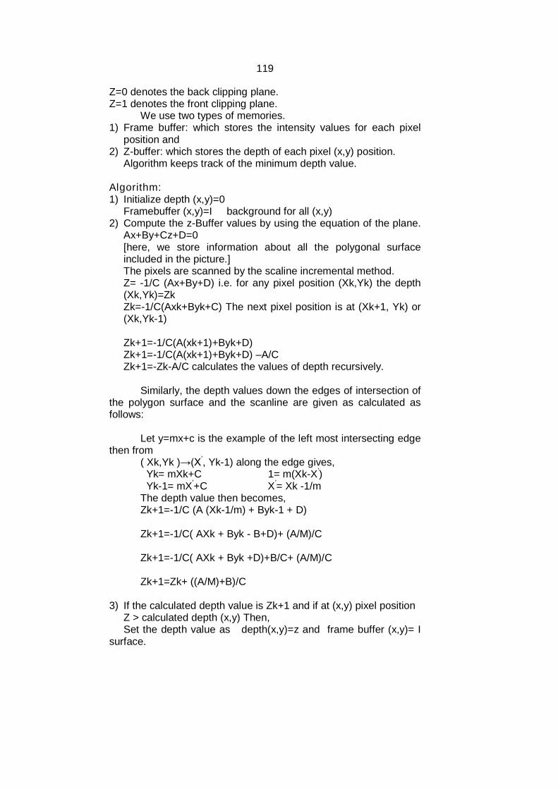
119

Z=0 denotes the back clipping plane.Z=1 denotes the front clipping plane.

We use two types of memories.1) Frame buffer: which stores the intensity values for each pixel

position and2) Z-buffer: which stores the depth of each pixel (x,y) position.

Algorithm keeps track of the minimum depth value.

Algorithm:1) Initialize depth (x,y)=0

Framebuffer (x,y)=I background for all (x,y)2) Compute the z-Buffer values by using the equation of the plane.

Ax+By+Cz+D=0[here, we store information about all the polygonal surfaceincluded in the picture.]The pixels are scanned by the scaline incremental method.Z= -1/C (Ax+By+D) i.e. for any pixel position (Xk,Yk) the depth(Xk,Yk)=ZkZk=-1/C(Axk+Byk+C) The next pixel position is at (Xk+1, Yk) or(Xk,Yk-1)

Zk+1=-1/C(A(xk+1)+Byk+D)Zk+1=-1/C(A(xk+1)+Byk+D) –A/CZk+1=-Zk-A/C calculates the values of depth recursively.

Similarly, the depth values down the edges of intersection ofthe polygon surface and the scanline are given as calculated asfollows:

Let y=mx+c is the example of the left most intersecting edgethen from

( Xk,Yk )→(X’, Yk-1) along the edge gives,Yk= mXk+C 1= m(Xk-X’)Yk-1= mX’+C X’= Xk -1/m

The depth value then becomes,Zk+1=-1/C (A (Xk-1/m) + Byk-1 + D)

Zk+1=-1/C( AXk + Byk - B+D)+ (A/M)/C

Zk+1=-1/C( AXk + Byk +D)+B/C+ (A/M)/C

Zk+1=Zk+ ((A/M)+B)/C

3) If the calculated depth value is Zk+1 and if at (x,y) pixel positionZ > calculated depth (x,y) Then,Set the depth value as depth(x,y)=z and frame buffer (x,y)= I

surface.

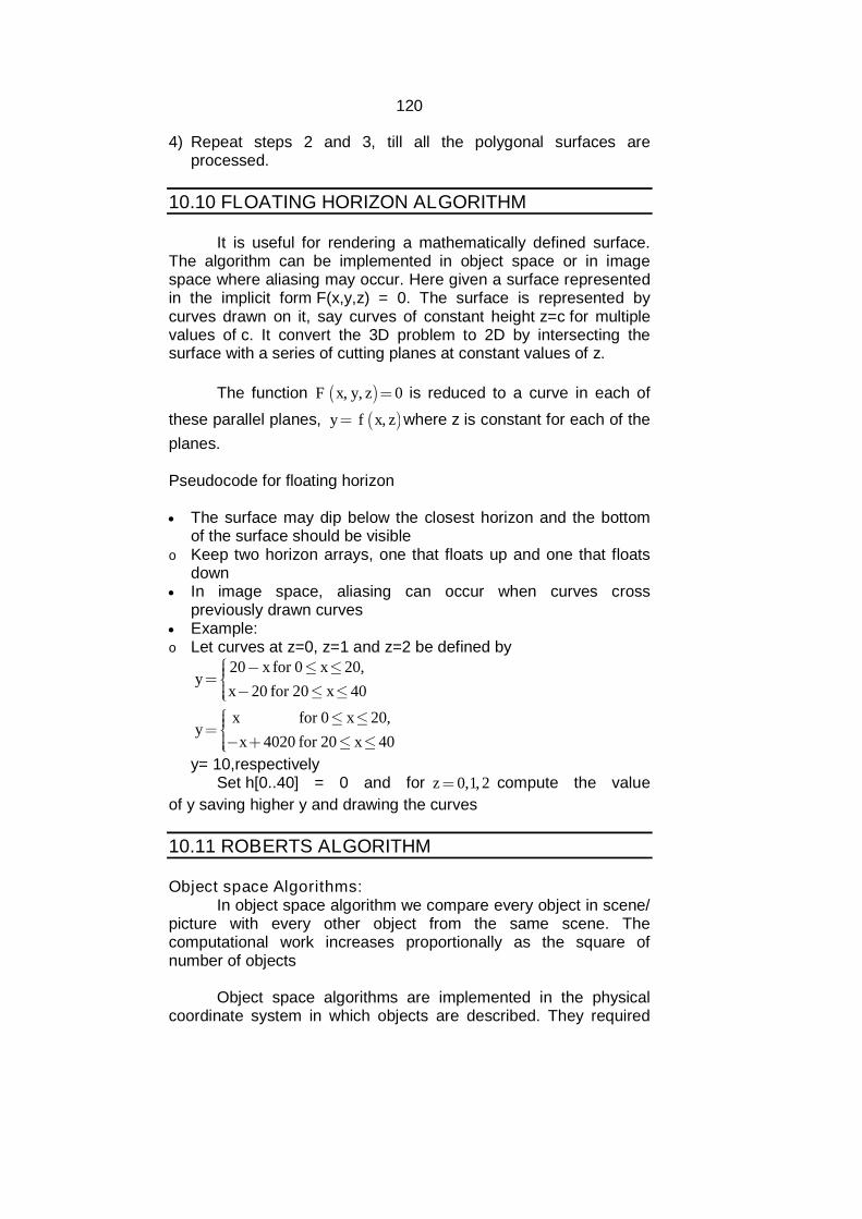
120

4) Repeat steps 2 and 3, till all the polygonal surfaces areprocessed.

10.10 FLOATING HORIZON ALGORITHM

It is useful for rendering a mathematically defined surface.The algorithm can be implemented in object space or in imagespace where aliasing may occur. Here given a surface representedin the implicit form F(x,y,z) = 0. The surface is represented bycurves drawn on it, say curves of constant height z=c for multiplevalues of c. It convert the 3D problem to 2D by intersecting thesurface with a series of cutting planes at constant values of z.

The function , , 0F x y z is reduced to a curve in each of

these parallel planes, ,y f x z where z is constant for each of the

planes.

Pseudocode for floating horizon

The surface may dip below the closest horizon and the bottomof the surface should be visible

o Keep two horizon arrays, one that floats up and one that floatsdown

In image space, aliasing can occur when curves crosspreviously drawn curves

Example:o Let curves at z=0, z=1 and z=2 be defined by

20 for 0 20,

20 for 20 40

for 0 20,

4020 for 20 40

x xy

x x

x xy

x x

y= 10,respectivelySet h[0..40] = 0 and for 0,1, 2z compute the value

of y saving higher y and drawing the curves

10.11 ROBERTS ALGORITHM

Object space Algorithms:In object space algorithm we compare every object in scene/

picture with every other object from the same scene. Thecomputational work increases proportionally as the square ofnumber of objects

Object space algorithms are implemented in the physicalcoordinate system in which objects are described. They required

121

less storage space. They are particularly useful in engineeringapplications.

The object space algorithm is Robert’s Algorithm.It gives elegant mathematical solution which is operated in

object space because of more efficient image space algorithm.Roberts’s algorithm is less appreciated. It requires each scene tobe divided into volumes which are either convex or concave. Thesevolumes are further divided to component volumes.

This algorithm is developed in 3 parts. 1st part analysis each part separately to eliminate the hidden

plane. 2nd part compares remaining edges of each volume against all

other to find which line segments are hidden 3rd part construct the junction lines for penetrating volume.

Algorithm assumes that a volume consists of planepolygonal faces. The faces consist of edges and the edges consistof individual vertices.

Algorihtm:1. { start

Eliminate the hidden plane{2. For each volume in the scene{3.

i) form volume matrix listii) compute the equation of plane for each face polygon of the

volume.iii) Check the sign of the plane equation.iv) find a point which lies inside the volume and find the dot

product of the equation of plane with this point. If the dotproduct is less than zero change the sign of the planeequation.

v) form the modified volume matrix.vi) Multiply by the inverse of the viewing transformation.vii) Compute and store the bounding box values as Xmin, Xmax,

Ymin, Ymax, Zmin, Zmax for the transformation volume.1. Identify the hidden plane.{

i) Take the dot product of test point at infinity and transformvolume matrix.

ii) If the dot product is < 0 then the plane is the hidden plane.iii) Eliminate entire polygon forming that plane. This eliminates

the necessity for separately identifying hidden lines.}

2. Eliminate the line segments for each volume hidden by on othervolume in the scene.If there is only one volume ---- STOP.Else

122

For a priority list of volumes by performing any efficientsorting algorithm on the z- coordinate

For each volume in the sorted listDO {

i) Test the self hidden edges against all other volumes.ii) The volume whose edges are being tested is named as the test

object which is tested against the current test volume.iii) Perform bounding box test. For the test object and test volume.

As follows: {If Xmin(test vol) > Xmax(test obj)OR Xmax(test vol) < Xmin(test obj)OR Ymin(test vol) > Ymax(test obj)OR Ymax(test vol) < Ymin(test obj) Then

The test volume cannot hide any edge of the objectContinue with the next test volume.

Else perform preliminary penetrating text to click if the testobject is in sorted in the test volume.

[if the insertion list is empty No insertion.]3. Determine the visible junction lines for penetrating volumes.

If the visibility False, Skip through the display routine.If no penetrating points have been recorded, Skip through thedisplay routine.Form possible junction edges by connections all penetratingpoints.Test all junction edges against the both volumes.Test the surviving visible junction edges against all volumes inthe scene for visibility. Save the visible segments.

4. Display remaining visible edges5. } End.


1. Which stores the intensity values for each pixel position isknown as _______.

2. Which stores the depth of each pixel (x,y) position is known as___________.

10.12 LET US SUM UP

The bilinear surface is the simplest non flat (curved) surfacebecause it is fully defined by means of its four corner points

The translation sweep and rotational sweep is combined to get a3D object. The corresponding sweep representation is called asgeneral sweep.

123

The problem of removing the unwanted surfaces and line iscalled “hidden surface problem”.

Back-face culling directly eliminates polygons not facing theviewer.



Computer Graphics, ISRD Group, Tata McGraw Hill. Computer Graphics, Amarendra Sinha, A. Udai,, Tata McGraw

Hill. Computer Graphics,A. P. Godase, Technical Publications Pune. Mathematical Elements of Computer Graphics, David F. Rogers,

Tata McGraw Hill. Computer Graphics, Donald Hearn, M P. Baker, PHI. Computer Graphics: A programming Approach, Steven

Harrington, McGraw-Hill. Theory and Problems of Computer Graphics, Zhigang Xiang,

Roy, plastock, Schaum’s outline series, McGraw-Hill.

10.14 EXERCISE

1. What is hidden surface problem? Discuss in brief.2. Explain the following models: a) wireframe b) sweep

representation3. What is painter’s algorithm? Explain with an example.4. Give the z-buffer algorithm and explain it.5. What is Back-face culling?6. Explain the steps in Robert’s algorithm.7. How to construct Bezier Surface?

124

11

OBJECT RENDERING

Unit Structure:

11.0 Objectives

11.1 Introduction

11.2 Light Modeling Techniques

11.3 Illumination Model

11.4 Shading:

11.4.1 Flat Shading

11.4.2 Polygon Mesh Shading

11.4.3 Gaurand Shading Model

11.4.4 Phong Shading

11.5 Transparency Effect

11.6 Shadows

11.7 Texture and Object Representation

11.8 Ray Tracing

11.9 Ray Casting

11.10 Radiosity

11.11 Color Models

11.12 Let us sum up


11.14 Exercise

11.0 OBJECTIVE

The objective of this chapter is To understand light modeling techniques and illumination

models. To understand different types of shading models. To understand concepts Ray Tracing and Radiosity.

11.1 INTRODUCTION

We know that the realistic scenes are obtained bygenerating transformations, perceptive projection of objects and by

125

applying lighting effects to the visible surface. An illumination modelis used to calculate the intensity of light that we are going to see ata given point on the surface of an object. Illumination models arealso some time called as lighting or shading models. Here, weconsider shading of 3-D objects and its models. In illuminationmodels to calculate the intensity of the color we use the method ofthe object rendering.

11.2 LIGHT MODELING TECHNIQUES

The object may be illuminated by light which can come fromall direction.

A surface that is not exposed directly to a light source will bestill visible if nearby objects are illuminated. In basic illuminationmodel we can set a general level of brightness of a scene. Themethod by which we create such effect usually follows the laws ofreflections. The light reflections obtained from various surfaces topproduce a uniform illumination is called ambient light or backgroundlight. It has no special or directional characteristics the amount ofambient light incident on each object is constant for all the surfacesand for all the direction. When the illumination is uniform from alldirections it is called ‘diffused illumination’. Usually diffusedillumination is a back ground light which is reflected from wallsscenes and curve ceiling, floor.

When we illuminate a shiny surface such as polish metal weobserve highlight or bright spot on the shining surface. Thisphenomenon of reflection of light in concentrated area around thereflection angle is called specular reflection. Due to specularreflection the surface appears to be not in its original color butwhite, the color of the incident light. The specular reflection angle isalways equal to the angle of incident light.

11.3 ILLUMINATION MODEL

An illumination or lighting model is a model or technique fordetermining the colour of a surface of an object at a given point. Asimple illumination model can be based on three components:ambient reflection, diffuse reflection and specular reflection.

11.4 SHADING

A shading model is used in computer graphics to simulatethe effects of light shining on a surface. The intensity that we seeon a surface is dependent upon two things one the type of lightsources and second the surface characteristics (eg. Shining, matte,dull, and opaque or transparent).

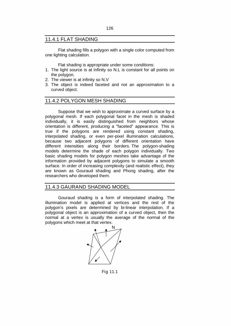
126

11.4.1 FLAT SHADING

Flat shading fills a polygon with a single color computed fromone lighting calculation.

Flat shading is appropriate under some conditions:1. The light source is at infinity so N.L is constant for all points on

the polygon.2. The viewer is at infinity so N.V3. The object is indeed faceted and not an approximation to a

curved object.

11.4.2 POLYGON MESH SHADING

Suppose that we wish to approximate a curved surface by apolygonal mesh. If each polygonal facet in the mesh is shadedindividually, it is easily distinguished from neighbors whoseorientation is different, producing a "faceted" appearance. This istrue if the polygons are rendered using constant shading,interpolated shading, or even per-pixel illumination calculations,because two adjacent polygons of different orientation havedifferent intensities along their borders. The polygon-shadingmodels determine the shade of each polygon individually. Twobasic shading models for polygon meshes take advantage of theinformation provided by adjacent polygons to simulate a smoothsurface. In order of increasing complexity (and realistic effect), theyare known as Gouraud shading and Phong shading, after theresearchers who developed them.

11.4.3 GAURAND SHADING MODEL

Gouraud shading is a form of interpolated shading. Theillumination model is applied at vertices and the rest of thepolygon’s pixels are determined by bi-linear interpolation. If apolygonal object is an approximation of a curved object, then thenormal at a vertex is usually the average of the normal of thepolygons which meet at that vertex.

N

Fig 11.1

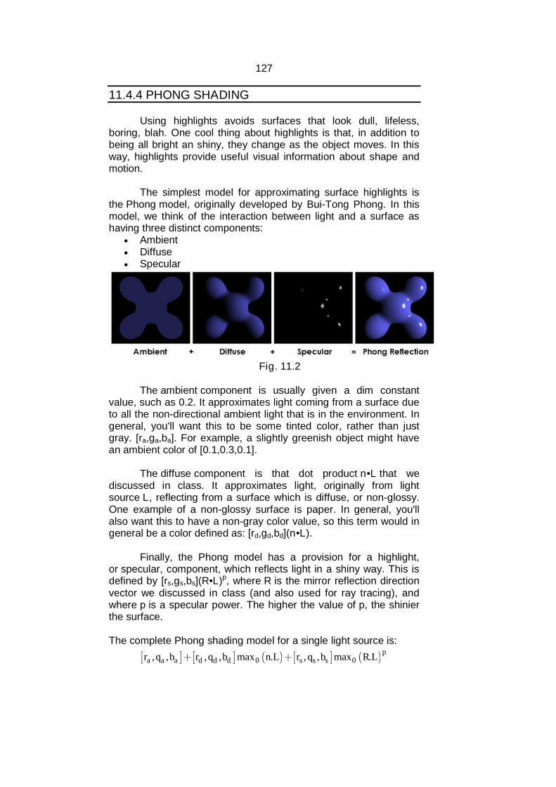
127

11.4.4 PHONG SHADING

Using highlights avoids surfaces that look dull, lifeless,boring, blah. One cool thing about highlights is that, in addition tobeing all bright an shiny, they change as the object moves. In thisway, highlights provide useful visual information about shape andmotion.

The simplest model for approximating surface highlights isthe Phong model, originally developed by Bui-Tong Phong. In thismodel, we think of the interaction between light and a surface ashaving three distinct components:

Ambient Diffuse Specular

Fig. 11.2

The ambient component is usually given a dim constantvalue, such as 0.2. It approximates light coming from a surface dueto all the non-directional ambient light that is in the environment. Ingeneral, you'll want this to be some tinted color, rather than justgray. [ra,ga,ba]. For example, a slightly greenish object might havean ambient color of [0.1,0.3,0.1].

The diffuse component is that dot product n•L that wediscussed in class. It approximates light, originally from lightsource L, reflecting from a surface which is diffuse, or non-glossy.One example of a non-glossy surface is paper. In general, you'llalso want this to have a non-gray color value, so this term would ingeneral be a color defined as: [rd,gd,bd](n•L).

Finally, the Phong model has a provision for a highlight,or specular, component, which reflects light in a shiny way. This isdefined by [rs,gs,bs](R•L)p, where R is the mirror reflection directionvector we discussed in class (and also used for ray tracing), andwhere p is a specular power. The higher the value of p, the shinierthe surface.

The complete Phong shading model for a single light source is:

0 0, , , , max . , , max .p

a a a d d d s s sr q b r q b n L r q b R L

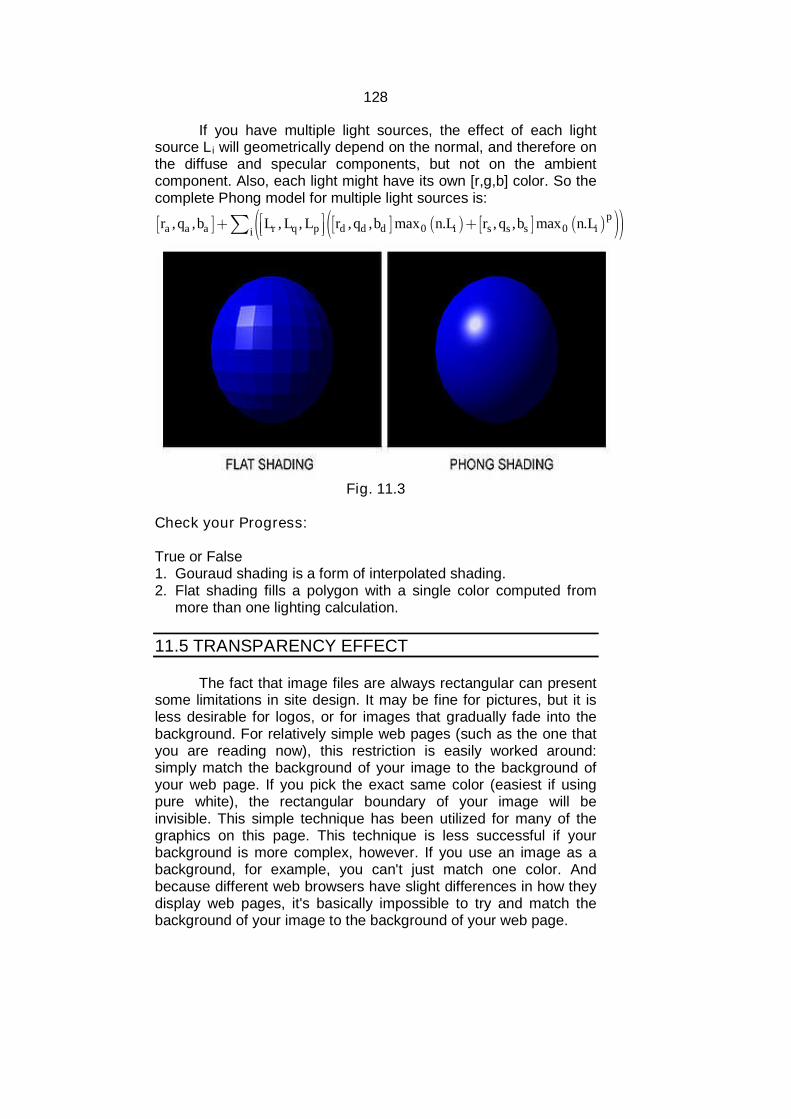
128

If you have multiple light sources, the effect of each lightsource Li will geometrically depend on the normal, and therefore onthe diffuse and specular components, but not on the ambientcomponent. Also, each light might have its own [r,g,b] color. So thecomplete Phong model for multiple light sources is:

0 0, , , , , , max . , , max .p

a a a r q p d d d i s s s iir q b L L L r q b n L r q b n L

Fig. 11.3


True or False1. Gouraud shading is a form of interpolated shading.2. Flat shading fills a polygon with a single color computed from

more than one lighting calculation.

11.5 TRANSPARENCY EFFECT

The fact that image files are always rectangular can presentsome limitations in site design. It may be fine for pictures, but it isless desirable for logos, or for images that gradually fade into thebackground. For relatively simple web pages (such as the one thatyou are reading now), this restriction is easily worked around:simply match the background of your image to the background ofyour web page. If you pick the exact same color (easiest if usingpure white), the rectangular boundary of your image will beinvisible. This simple technique has been utilized for many of thegraphics on this page. This technique is less successful if yourbackground is more complex, however. If you use an image as abackground, for example, you can't just match one color. Andbecause different web browsers have slight differences in how theydisplay web pages, it's basically impossible to try and match thebackground of your image to the background of your web page.

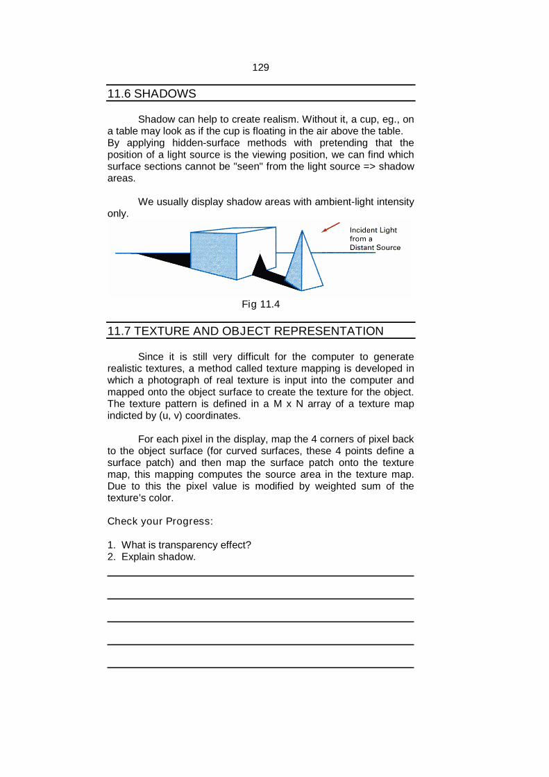
129

11.6 SHADOWS

Shadow can help to create realism. Without it, a cup, eg., ona table may look as if the cup is floating in the air above the table.By applying hidden-surface methods with pretending that theposition of a light source is the viewing position, we can find whichsurface sections cannot be "seen" from the light source => shadowareas.

We usually display shadow areas with ambient-light intensityonly.

Fig 11.4

11.7 TEXTURE AND OBJECT REPRESENTATION

Since it is still very difficult for the computer to generaterealistic textures, a method called texture mapping is developed inwhich a photograph of real texture is input into the computer andmapped onto the object surface to create the texture for the object.The texture pattern is defined in a M x N array of a texture mapindicted by (u, v) coordinates.

For each pixel in the display, map the 4 corners of pixel backto the object surface (for curved surfaces, these 4 points define asurface patch) and then map the surface patch onto the texturemap, this mapping computes the source area in the texture map.Due to this the pixel value is modified by weighted sum of thetexture’s color.


1. What is transparency effect?2. Explain shadow.

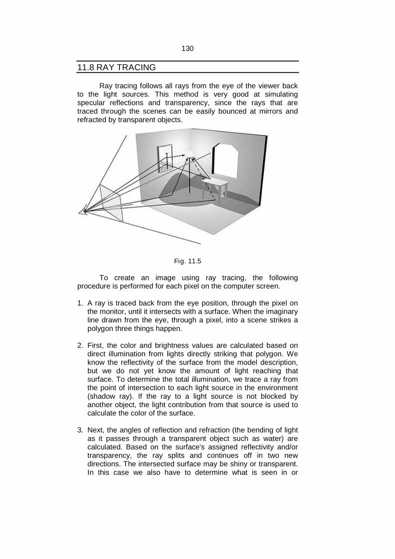
130

11.8 RAY TRACING

Ray tracing follows all rays from the eye of the viewer backto the light sources. This method is very good at simulatingspecular reflections and transparency, since the rays that aretraced through the scenes can be easily bounced at mirrors andrefracted by transparent objects.

Fig. 11.5

To create an image using ray tracing, the followingprocedure is performed for each pixel on the computer screen.

1. A ray is traced back from the eye position, through the pixel onthe monitor, until it intersects with a surface. When the imaginaryline drawn from the eye, through a pixel, into a scene strikes apolygon three things happen.

2. First, the color and brightness values are calculated based ondirect illumination from lights directly striking that polygon. Weknow the reflectivity of the surface from the model description,but we do not yet know the amount of light reaching thatsurface. To determine the total illumination, we trace a ray fromthe point of intersection to each light source in the environment(shadow ray). If the ray to a light source is not blocked byanother object, the light contribution from that source is used tocalculate the color of the surface.

3. Next, the angles of reflection and refraction (the bending of lightas it passes through a transparent object such as water) arecalculated. Based on the surface's assigned reflectivity and/ortransparency, the ray splits and continues off in two newdirections. The intersected surface may be shiny or transparent.In this case we also have to determine what is seen in or

131

through the surface being processed. Steps 1 and 2 arerepeated in the reflected (and, in the case of transparency,transmitted) direction until another surface is encountered. Thecolor at the subsequent intersection point is calculated andfactored into the original point.

4. If the second surface is yet again a reflective or transparentsurface, the ray tracing process repeats once again, and so on,until a maximum number of iterations is reached or until no moresurfaces are intersected. Each ray continues bouncing aroundthe scene until it hits a light source, leaves the scene, orreaches some arbitrary number (recursion level). When all therays have completed their journeys the intensity and colorvalues are combined and the pixel is painted.

11.9 RAY CASTING

The basic goal of ray casting is to allow the best use of thethree-dimensional data and not attempt to impose any geometricstructure on it. It solves one of the most important limitations ofsurface extraction techniques, namely the way in which they displaya projection of a thin shell in the acquisition space. Surfaceextraction techniques fail to take into account that, particularly inmedical imaging, data may originate from fluid and other materialswhich may be partially transparent and should be modeled as such.Ray casting doesn't suffer from this limitation.

11.10 RADIOSITY

There is a new method of rendering that was recentlydeveloped. It is called radiosity.

It does something all the other rendering methods don't do: itfigures out the relationship in the scene of all the objects present.For example, in real life, if you take a bright colored ball and put itinto a white room, the walls of the room are going to reflect a littlebit of color from the ball, making them look a little reddish forexample.

This is not possible in ray tracing, since it does not bouncerays off of matte objects, such as a wall. You can compare theabove picture to the one of the ray traced object. All though this isnot a very good example, you can see that the checkerboardpattern of the "tri-ball" has a slight effect on the color of the bricksright underneath it. This adds the extra thing to rendered scenesand makes them look extremely realistic. Radiosity producesextremely good results, but unfortunately, there is a tradeoff:rendering time. Before the computer even starts rendering, it has to

132

solve a certain "radiosity model" which is the relationship of oneobject on all the other ones in a scene. Then it can start rendering.

Check your progress:1. Give the procedure of ray tracing.2. What is radiosity?

11.11 COLOR MODELS

RGB Model:There are many different ways of specifying color, or color

models. The most common is the RGB color model where a color isspecified in terms of red, green and blue color components. If weuse the RGB color model then the ambient color (reflectivity) of anobject is (kaR, kaG, kaB), the diffuse color (reflectivity) of an objectkd is (kdR, kdG, kdB) and the color of the light emitted from thepoint light source as (LdR,LdG,LdB).

Fig. 11.6

CMY:It is possible to achieve a large range of colors seen by humans bycombining cyan, magenta, and yellow transparent dyes/inks on awhite substrate. These are the subtractive primary colors. Often afourth black is added to improve reproduction of some dark colors.This is called "CMY" or "CMYK" color space. The cyan ink absorbs

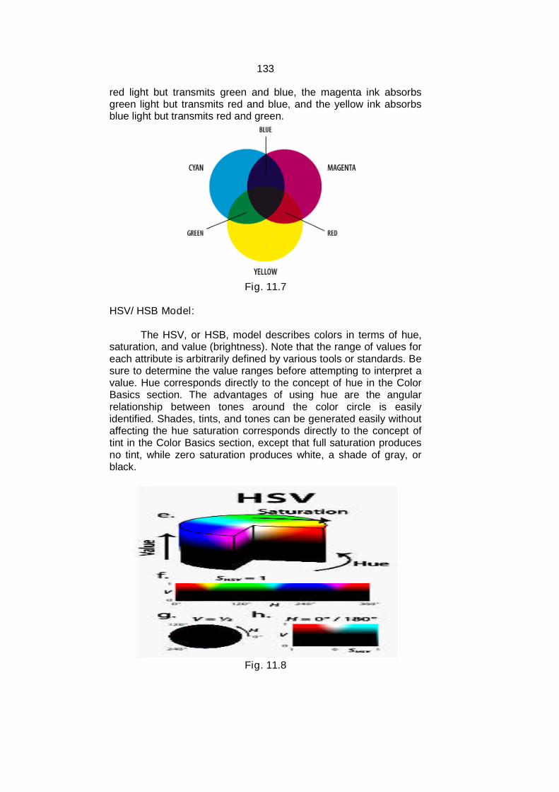
133

red light but transmits green and blue, the magenta ink absorbsgreen light but transmits red and blue, and the yellow ink absorbsblue light but transmits red and green.

Fig. 11.7

HSV/ HSB Model:

The HSV, or HSB, model describes colors in terms of hue,saturation, and value (brightness). Note that the range of values foreach attribute is arbitrarily defined by various tools or standards. Besure to determine the value ranges before attempting to interpret avalue. Hue corresponds directly to the concept of hue in the ColorBasics section. The advantages of using hue are the angularrelationship between tones around the color circle is easilyidentified. Shades, tints, and tones can be generated easily withoutaffecting the hue saturation corresponds directly to the concept oftint in the Color Basics section, except that full saturation producesno tint, while zero saturation produces white, a shade of gray, orblack.

Fig. 11.8

134

11.12 LET US SUM UP

When light sources create highlights or bright spots they arecalled ‘specular reflections’. This effect is usually seen onshining surfaces than on dull surfaces.

When the illumination is uniform from all directions it is called‘diffused illumination’.

Flat shading fills a polygon with a single color

Gouraud shading is a form of interpolated shading.




Mathematical Elements of Computer Graphics, David F. Rogers,Tata McGraw Hill.


11.13 EXERCISE

1. Write a short note on light modeling techniques.2. List the different types of shading. Explain any one in details.3. Write a short note on Phong shading.4. Write a short note on Gaurand Shading Model

135

12

INTRODUCTION TO ANIMATION

Unit Structure:

12.0 Objectives12.1 Introduction12.2 Key-Frame Animation12.3 Construction of an Animation Sequence12.4 Motion Control Methods12.5 Procedural Animation12.6 Key-Frame Animation vs. Procedural Animation12.7 Introduction to Morphing12.8 Three-Dimensional Morphing12.9 Let us sum up12.10 References and Suggested Reading12.11 Exercise

12.0 OBJECTIVE

The objective of this chapter is To understand the concepts of computer animation. To understand Morphing.

12.1 INTRODUCTION

The main goal of computer animation is to synthesize thedesired motion effect which is a mixing of natural phenomena,perception and imagination. The animator designs the object'sdynamic behavior with his mental representation of causality

12.2 KEY-FRAME ANIMATION

When someone creates an animation on a computer, theyusually don't specify the exact position of any given object on everysingle frame. They create key frames. Key frames are importantframes during which an object changes its size, direction, shape orother properties. The computer then figures out all the in betweenframes and saves an extreme amount of time for the animator. Twoframes are drawn by user In between frames generated bycomputer.

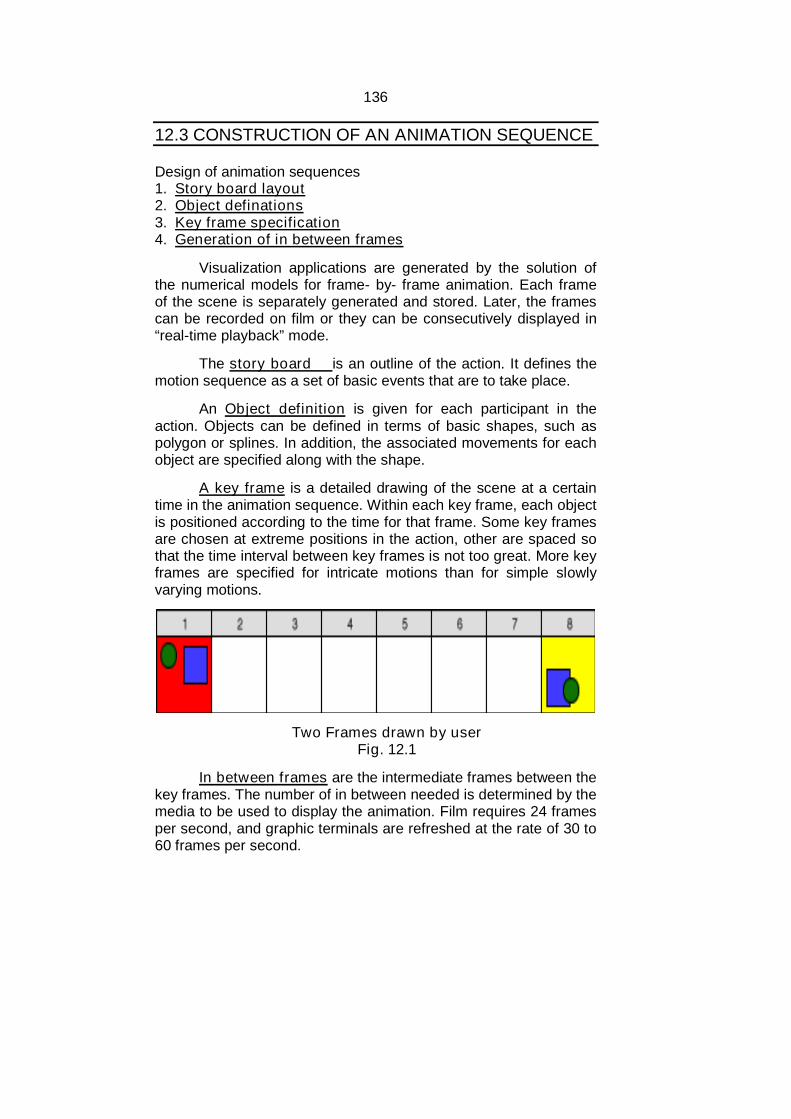
136

12.3 CONSTRUCTION OF AN ANIMATION SEQUENCE

Design of animation sequences1. Story board layout2. Object definations3. Key frame specification4. Generation of in between frames

Visualization applications are generated by the solution ofthe numerical models for frame- by- frame animation. Each frameof the scene is separately generated and stored. Later, the framescan be recorded on film or they can be consecutively displayed in“real-time playback” mode.

The story board is an outline of the action. It defines themotion sequence as a set of basic events that are to take place.

An Object definition is given for each participant in theaction. Objects can be defined in terms of basic shapes, such aspolygon or splines. In addition, the associated movements for eachobject are specified along with the shape.

A key frame is a detailed drawing of the scene at a certaintime in the animation sequence. Within each key frame, each objectis positioned according to the time for that frame. Some key framesare chosen at extreme positions in the action, other are spaced sothat the time interval between key frames is not too great. More keyframes are specified for intricate motions than for simple slowlyvarying motions.

Two Frames drawn by userFig. 12.1

In between frames are the intermediate frames between thekey frames. The number of in between needed is determined by themedia to be used to display the animation. Film requires 24 framesper second, and graphic terminals are refreshed at the rate of 30 to60 frames per second.

137

In between frames generated by computerFig. 12.2

Final AnimationFig. 12.3


Fill in the blanks.1. _________ frames are the intermediate frames between the key

frames.2. The ________is an outline of the action.3. _________ is a detailed drawing of the scene at a certain time in

the animation sequence.

12.4 MOTION CONTROL METHODS

The key issue of Computer Animation is the way of definingmotion, what is commonly known as Motion Control Methods(MCMs). MCMs may be classified based on the nature of theinformation, which is directly manipulated: geometric, physical, orbehavioral

Methods based on Geometric and Kinematics informationThese methods are heavily relied upon the animator. Motion

is locally controlled and defined in terms of coordinates, angles,velocities, or accelerations.

The Performance Animation which consists in magnetic oroptical measurement and recording of direct actions of a realperson for immediate or delayed playback. The technique is

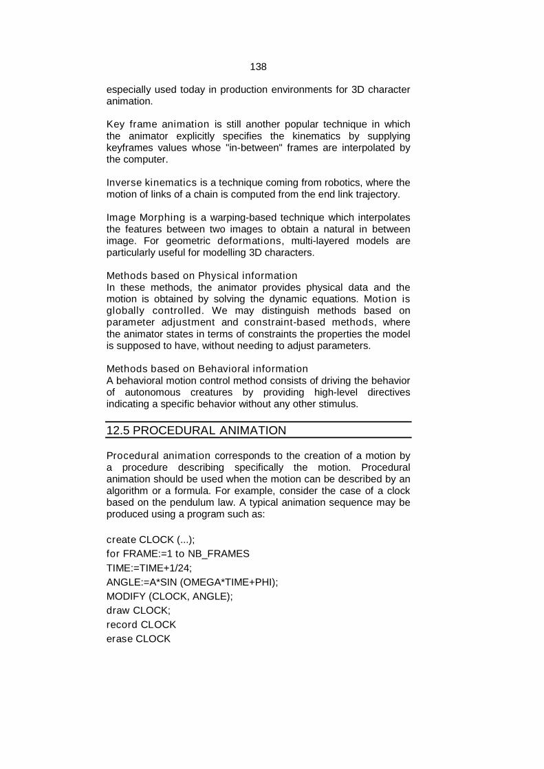
138

especially used today in production environments for 3D characteranimation.

Key frame animation is still another popular technique in whichthe animator explicitly specifies the kinematics by supplyingkeyframes values whose "in-between" frames are interpolated bythe computer.

Inverse kinematics is a technique coming from robotics, where themotion of links of a chain is computed from the end link trajectory.

Image Morphing is a warping-based technique which interpolatesthe features between two images to obtain a natural in betweenimage. For geometric deformations, multi-layered models areparticularly useful for modelling 3D characters.

Methods based on Physical informationIn these methods, the animator provides physical data and themotion is obtained by solving the dynamic equations. Motion isglobally controlled. We may distinguish methods based onparameter adjustment and constraint-based methods, wherethe animator states in terms of constraints the properties the modelis supposed to have, without needing to adjust parameters.

Methods based on Behavioral informationA behavioral motion control method consists of driving the behaviorof autonomous creatures by providing high-level directivesindicating a specific behavior without any other stimulus.

12.5 PROCEDURAL ANIMATION

Procedural animation corresponds to the creation of a motion bya procedure describing specifically the motion. Proceduralanimation should be used when the motion can be described by analgorithm or a formula. For example, consider the case of a clockbased on the pendulum law. A typical animation sequence may beproduced using a program such as:

create CLOCK (...);

for FRAME:=1 to NB_FRAMES

TIME:=TIME+1/24;

ANGLE:=A*SIN (OMEGA*TIME+PHI);

MODIFY (CLOCK, ANGLE);

draw CLOCK;

record CLOCK

erase CLOCK

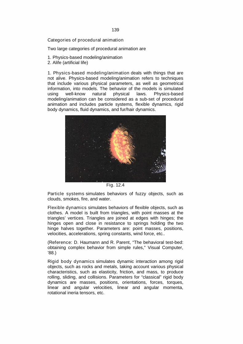
139

Categories of procedural animation

Two large categories of procedural animation are

1. Physics-based modeling/animation2. Alife (artificial life)

1. Physics-based modeling/animation deals with things that arenot alive. Physics-based modeling/animation refers to techniquesthat include various physical parameters, as well as geometricalinformation, into models. The behavior of the models is simulatedusing well-know natural physical laws. Physics-basedmodeling/animation can be considered as a sub-set of proceduralanimation and includes particle systems, flexible dynamics, rigidbody dynamics, fluid dynamics, and fur/hair dynamics.

Fig. 12.4

Particle systems simulates behaviors of fuzzy objects, such asclouds, smokes, fire, and water.

Flexible dynamics simulates behaviors of flexible objects, such asclothes. A model is built from triangles, with point masses at thetriangles’ vertices. Triangles are joined at edges with hinges; thehinges open and close in resistance to springs holding the twohinge halves together. Parameters are: point masses, positions,velocities, accelerations, spring constants, wind force, etc..

(Reference: D. Haumann and R. Parent, “The behavioral test-bed:obtaining complex behavior from simple rules,” Visual Computer,’88.)

Rigid body dynamics simulates dynamic interaction among rigidobjects, such as rocks and metals, taking account various physicalcharacteristics, such as elasticity, friction, and mass, to producerolling, sliding, and collisions. Parameters for “classical” rigid bodydynamics are masses, positions, orientations, forces, torques,linear and angular velocities, linear and angular momenta,rotational ineria tensors, etc.

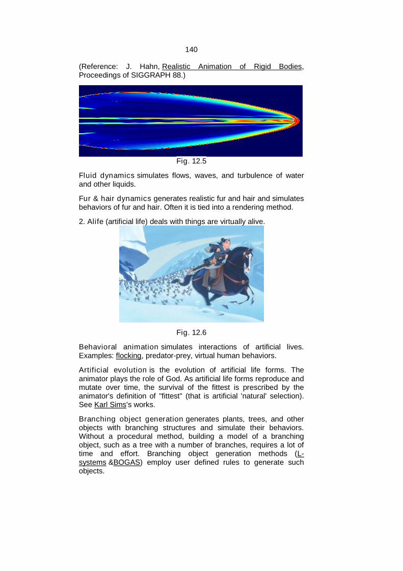
140

(Reference: J. Hahn, Realistic Animation of Rigid Bodies,Proceedings of SIGGRAPH 88.)

Fig. 12.5

Fluid dynamics simulates flows, waves, and turbulence of waterand other liquids.

Fur & hair dynamics generates realistic fur and hair and simulatesbehaviors of fur and hair. Often it is tied into a rendering method.

2. Alife (artificial life) deals with things are virtually alive.

Fig. 12.6

Behavioral animation simulates interactions of artificial lives.Examples: flocking, predator-prey, virtual human behaviors.

Artificial evolution is the evolution of artificial life forms. Theanimator plays the role of God. As artificial life forms reproduce andmutate over time, the survival of the fittest is prescribed by theanimator's definition of "fittest" (that is artificial 'natural' selection).See Karl Sims's works.

Branching object generation generates plants, trees, and otherobjects with branching structures and simulate their behaviors.Without a procedural method, building a model of a branchingobject, such as a tree with a number of branches, requires a lot oftime and effort. Branching object generation methods (L-systems &BOGAS) employ user defined rules to generate suchobjects.

141

12.6 KEY-FRAME ANIMATION VS. PROCEDURALANIMATION

In a procedural animation objects are animated by aprocedure -- a set of rules -- not by keyframing. The animatorspecifies rules and initial conditions and runs simulation. Rules areoften based on physical rules of the real world expressed bymathematical equations.

To produce a keyframe animation, the animator creates thebehavior of a model manually by using an intuitive “put that there”methodology. The animator has direct control over the positions,shapes, and motions of models at any moment in the animation. Onthe other hand, to produce a procedural animation the animatorprovides initial conditions and adjusts rather abstract physicalparameters, such as forces and torques, in order to controlpositions, shapes, and motions of models. The effect of changing aparameter value is often unpredictable in procedural animation. Theanimator has to run a simulation to see the result.


1. What are motion control methods?2. Explain procedural animation.

12.7 INTRODUCTION TO MORPHING

Morphing is a special effect in motion pictures andanimations that changes (or morphs) one image into anotherthrough a seamless transition. Image morphing means creating asequence of images which when played in sequence, show oneimage being slowly changed into another image.

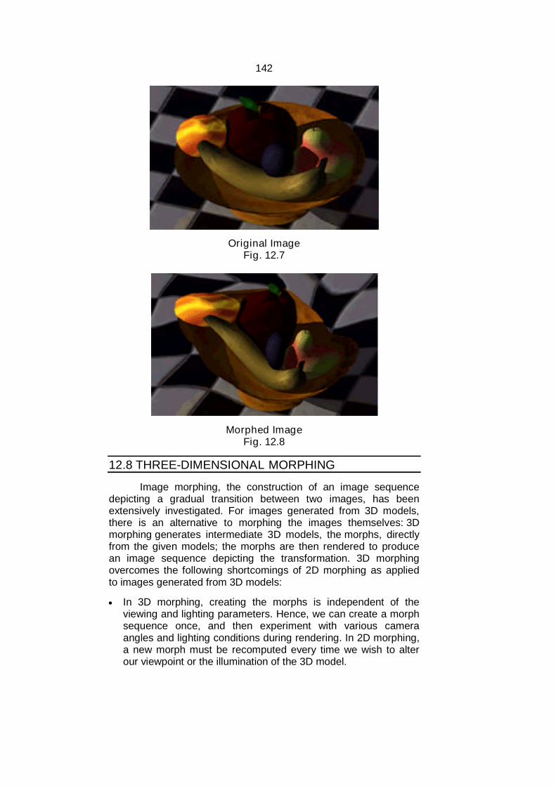
142

Original ImageFig. 12.7

Morphed ImageFig. 12.8

12.8 THREE-DIMENSIONAL MORPHING

Image morphing, the construction of an image sequencedepicting a gradual transition between two images, has beenextensively investigated. For images generated from 3D models,there is an alternative to morphing the images themselves: 3Dmorphing generates intermediate 3D models, the morphs, directlyfrom the given models; the morphs are then rendered to producean image sequence depicting the transformation. 3D morphingovercomes the following shortcomings of 2D morphing as appliedto images generated from 3D models:

In 3D morphing, creating the morphs is independent of theviewing and lighting parameters. Hence, we can create a morphsequence once, and then experiment with various cameraangles and lighting conditions during rendering. In 2D morphing,a new morph must be recomputed every time we wish to alterour viewpoint or the illumination of the 3D model.

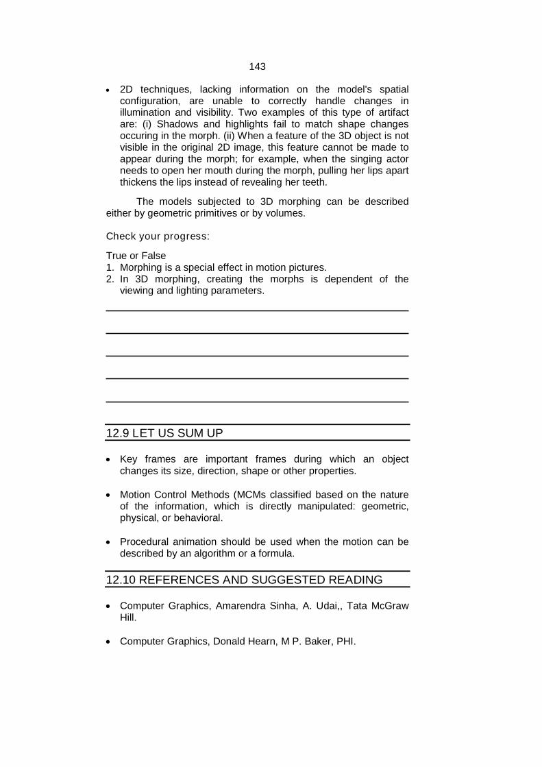
143

2D techniques, lacking information on the model's spatialconfiguration, are unable to correctly handle changes inillumination and visibility. Two examples of this type of artifactare: (i) Shadows and highlights fail to match shape changesoccuring in the morph. (ii) When a feature of the 3D object is notvisible in the original 2D image, this feature cannot be made toappear during the morph; for example, when the singing actorneeds to open her mouth during the morph, pulling her lips apartthickens the lips instead of revealing her teeth.

The models subjected to 3D morphing can be describedeither by geometric primitives or by volumes.


True or False1. Morphing is a special effect in motion pictures.2. In 3D morphing, creating the morphs is dependent of the

viewing and lighting parameters.

12.9 LET US SUM UP

Key frames are important frames during which an objectchanges its size, direction, shape or other properties.

Motion Control Methods (MCMs classified based on the natureof the information, which is directly manipulated: geometric,physical, or behavioral.

Procedural animation should be used when the motion can bedescribed by an algorithm or a formula.




144

Computer Graphics: A programming Approach, StevenHarrington, McGraw-Hill.

Theory and Problems of Computer Graphics, Zhigang Xiang,Roy, plastock, Schaum’s outline series, McGraw-Hill.

12.11 EXERCISE

1. Explain conventional animation.2. Write a short note on virtual reality.3. Write a short note on image morphing.4. Give the methods of controlling animation.5. What is frame by frame animation?6. Differentiate between Key-Frame Animation and Procedural

Animation.

Documents

Syllabus S.Y.B.Sc. (IT) SEMESTER - III, PAPER - II