1

S.Y. B.Sc. (IT) : Sem. III Data Structures

Time : 2½ Hrs.] Prelim Question Paper Solution [Marks : 75

Q.1 Attempt the following (any THREE) [15]Q.1(a) What is algorithm and explain by on Notation? [5](A) The term ‘algorithm’ refers to the sequence of instructions that must be followed to solve a

problem. In other words, an algorithm is a logical representation of the instructions which should be executed to perform a meaningful task.

An algorithm has certain characteristics. These are as follows : Each instruction should be unique and concise. Each instruction should be relative in nature and should not be repeated infinitely. Repetition of same task(s) should be avoided. The result should be available to the user after the algorithm terminates. Thus, an algorithm is any well defined computational procedure, along with a specified set of

allowable inputs, that produce some value or set of values as output. After an algorithm has been designed, its efficiency must be analyzed. This involves

determining whether the algorithm is economical in the use of computer resources. i.e. CPU time and memory. The term used to refer to the memory required by an algorithm is memory space and the term used to refer to the computational time is the running time.

The importance of efficiency of an algorithm is in the correctness that is, does it always

produce the correct result, and program complexity which considers both the difficulty of implementing an algorithm along with its efficiency.

Q.1(b) Explain sorting of array. [5](A) /*Program to accept numbers and sort them in ascending order using bubble sort*/ # include<stdio.h> main( ) { int n. i. j. arr[10]. temp : print f(“Enter how many numbers :”) : scanf (“ %d”, &n) : for (i = 0 : i<n : i++) { print f(“ enter the numbers%d : “, i+1): scanf(“%d” . &arr[i]) : } for (i=0 : i<n : i++) for (j=0 : J<n : j++) { i f(arr[j]>arr[j+1]) { temp=arr[j] : arr[j]=arr[j+1] : arr[j+1]=temp : } } printf (“Sorted numbers are : \n”) : for(i = 0 : i<n : i++)

Vidyalankar : S.Y. B.Sc. (IT) DS

2

print f(“%d ”. arr[i]) : print f(“\n”) : } / If the entered numbers are 23 15 29 11 1 the program will show the following output : Sorted numbers are : 1 11 15 23 29 Q.1(c) Explain two dimensional array. [5](A) A twodimensional array is a collection of elements placed in m rows and n columns. There

are two subscripts in the syntax of 2D array in which one specifies the number of rows and the other the number of columns. In a twodimensional array each element is itself an array.

The twodimensional array is also called a matrix. Manthematically, a matrix A is a collection

of elements ‘aij’ for all i and j’s such that 0 i<m and 0<j n. A matrix is said to be of order m n. A matrix can be conveniently represented by a twodimensional array. The various operations that can be performed on a matrix are : addition, multiplication, transposition, and finding the determinant of the matrix.

An example of 2D array can be arr [2][3] containing 2 rows and 3 columns and arr[0] [1] is

an element placed at 0th row and 1at column in the array. A twodimensional array can thus be represented as given in Fig.

A twodimensional array differentiates between the logical and physical view of data. A 2D array is a logical data structure that is useful in programming and problem solving. For example, such an array is useful in describing an object that is physically twodimensional such as a map or checkerboard.

Q.1(d) Explain different types of data structures. [5](A) Data Structure : Data Structure is the way of organizing data in such a way that the

retrieval of data becomes convenient. The journey of data structures start form fundamentals data types as they are the first

facility provided by the language to store data. Due to the increasing needs, the size and variety of data, data structures have gone ahead with derived data types, linear and finally non-linear data structures. Let us take a brief look on the various types of data structures.

Types of Data Structures 1) Primitive Data Structures : These are the default data types provided by the specific

language. For example, C language provides int, float, char etc., which can be used to store simple primary level data. For basic programming, these data types are more than sufficient for the management of data but as the level of programming increases, these data types normally are not used directly but are combined to form more complex data structures of the different types. We also form array and structures from these primitive types that are known as derived data types.

2) Linear Data Structures : The data structure where all the elements are stored in a

linear sequence is known as Linear Data Structure. Here all elements are of same

Prelim Paper Solution

3

hierarchy or level. For examples array and structure falls under the linear category which we have already studied. Now we are going to study stack, queue, linked list which are also considered as linear data structures.

Such data structures are limited when the system only uses same level of data. But in many situations we require to store data with hierarchy or level, for example directory structure. In such cases we need to take the help of non-linear data structures.

3) Non-Linear Data Structures : The data structure in which the data is stored with

hierarchy is known as Non-Linear Data Structure. All elements in this are not at same level. These are very useful when we have to store data with precedence or hierarchy. Some nonlinear data structures that we are going to study are binary tree and graph.

The various operations performed on the data structures are as follows: Traversing : The process of visiting each and every element of a data structure. Insertion : Adding new elements to the set of existing elements of a data structure. Deletion : Removing the existing elements from a data structure. Sorting : Arranging the elements of the data structure in the given order or

sequence. Searching : Finding the required element in the set of elements of a data structure. Q.1(e) Explain insertion and deletion in array. [5](A) Arrays are preferred for situations which require similar type of data items to be stored

together. An array is a finite collection of similar elements stored in adjacent memory locations. By

finite we mean that there are specific number of elements in an array and similar implies that all the elements in an array are of the same type. For example, an array may contain all integers of all characters.

Thus, an array is a collection of variables, of the same type that are referred by a common

name. The elements of the array are referenced respectively by an index set containing n consecutive numbers. An array with a number of elements is referenced using an index that ranges from 0 to n1. The lowest index of an array is called its range. The elements of an array arr[n]. containing n elements are referenced as arr[0], arr[2],… arr[n1] where 0 is the lower bound and ‘n1’ is the upper bound of the array.

Q.1(f) Explain abstract data type. [5](A) An Abstract Data Type (ADT) is defined as a mathematical model of the data objects that

make up a data type as well as the functions that operate on these objects. An abstract data type is the specification of logical and mathematical properties of a data type or structure. ADT acts as a useful guideline to implement a data type correctly. The specification of an ADT does not imply any implementation consideration. The implementation of an ADT involves the translation of the ADT’s specification into syntax of a particular programming language. The important step is the definition of ADT that involves mainly two parts :

1. Description of the way in which components are related to each other 2. Statements of operations that can be performed on that data type. For example, the int data type, available in the ‘C’ programming language provides an

implementation of the mathematical concept of an integer number. The int data type in ‘C’ can be considered as an implementation of Abstract Data Type, INTEGERADT. INTEGERADT defines the set of numbers given by the union of the set {1, 2, 3, …. } and the set of whole numbers {0, 1, …. + ). INTEGERADT also specifies the operations that can be performed on an integer number, for example addition, subtraction,

Vidyalankar : S.Y. B.Sc. (IT) DS

4

multiplication, etc. In the specification of the INTEGERADT. Following issues must be considered :

Range of numbers that will be represented. Format for storing the integer numbers.

This determines the representation of a signed integer value. Q.2 Attempt the following (any THREE) [15]Q.2(a) Explain how to insert the element in beginning of linked list. [5](A) Insertion in a linked list can be done in the following two ways: Insertion at the Beginning of the list Suppose we already have 5 nodes in the list and wish

to insert a new node in the beginning of the list. /*Function to insert a new node at the beginning of the linked list*/ void add_beg(struct node **q. int no) { struct node *temp : /* add new node */ temp malloc(sizeof(struct node)) : temp > data = no : temp > next = *q : t *q = temp : } From the figure given above it can be seen that a temp variable of structure type is taken and

space is allocated for this element using ‘malloc’ function and its data part contains the element or number and its link points to the existing first node.

Q.2(b) Explain deletion of a specified node in a linked list. [5](A) The process of deleting an element from a list is depicted in below Fig. In the following function, we traverse through the entire linked list, checking at each node

whether it has to be deleted. If the node being deleted is the first node then we shift the structure type pointer variable to the next node and then delete the earlier node.

If the node to be deleted is an intermediate node then the various pointers the links

before and after the deletion should be taken care of.

/* Function to Delete the specified node from the linked list */ void del(struct node **q. int no) {

Fig.: Insertion at the Beginning of the list

Fig. Deletion in Linked List

Prelim Paper Solution

5

struct node *old. *temp : temp = *q : while(temp : = NULL) { if (temp > data ==no) { /* If node to be deleted is the first node in the linked list */ if (temp ==*q) *q = temp > next : /* Deletes the intermediate node from the linked list */ else old > next = temp > next : /* Free the memory occupied by the node */ free(temp) : return : } /* Traverse the linked list till the last node is reached */ else { old = temp : /* old points to the previous node */ temp = temp > next : /* go to the next node */ } } printf(“\nElement %d not found”. no) : } Q.2(c) Explain Searching in Linked List. [5](A) Searching means finding information in a given linked list. /* Search a node with a given information */ void search (struct node *nodel) { int node_number = 0: int search_node : int flag = 0: nodel = &start : printf(*\n Input information of a node we want to search: =) : scanf(“%d” . & search_node) : if(nodel ==NULL) { printf(“\n List is empty) : } while(nodel) { if (search_node == node >data) { printf(“\n Search is successful”):

printf(“\n Information which we want to search is : %d”. search_node): printf(“\n Position from beginning of the list : %d”. node_number+1):

nodel = nodel > next : flag = 1 : }

Vidyalankar : S.Y. B.Sc. (IT) DS

6

else { nodel = nodel > next : } node_number ++: } if (!flag) { printf(“\n Search is unsuccessful”) : printf(“\n Information does not exist in the list: %d”. search_node): } } Q.2(d) Explain memory allocation and de-allocation in linked list. [5](A) C language requires us to specify the number of elements in an array at compile time. This

may cause wastage of memory space. Such situations can be taken care of by using dynamic data structures.

Dynamic memory management techniques allow us to allocate additional memory space or to release unwanted space at run time, thus, optimizing the use of storage space.

The memory management functions that can be used for allocating and freeing memory during

program execution are : * malloc Allocates requested size of bytes * calloc Allocates space for an array of elements * free Frees previously allocated space * realloc Modifies the size of previously allocated space. Q.2(e) Explain circular linked list. [5](A) A linked list in which last node points to the header node is called the circular linked list.

The circular linked lists have neither a beginning nor an end. A small change in the structure of linear linked list is made, that is, the next field in the last node contains a pointer back to the first node rather than the NULL pointer. Therefore, the structure defined for circular linked list is same as for the linear linked list as given below :

struct node { int data : struct node * next : } A shortcoming of the linear linked list is that with a given pointer to a node in linked list we

cannot reach and of the nodes that precede the node which the given pointer variable is pointing to. This disadvantage is overcome by making a little change in the structure of linear linked list and thus making a circular linked list as shown in Fig.

A circular linked list can be used to represent a stack and a queue. The following program

implements queue as a circular linked list. Pointers front and rear point to the first and last nodes of the list respectively.

Q.2(f) Explain Representation of Sparse Matrixes. [5](A) The sparse matrix can also be represented using a linked list. An element of sparse matrix

consists of three integers

Fig.

Prelim Paper Solution

7

it row number (i) its column number (j) and its value (val) In linked representation, consider “head” nodes for each row and each column pointing to

the elements in a particular row or column. A head node for a new consists of three parts (Fig.)

Row number indicates the row to which the “head” node is pointing to by component

“Element”. The head node also points to another “head” node for the next row. The structure definition for Rowhead is typedef struct Rowhead { int rownum : Element * right : struct Rowhead * next : } Row : Similarly, a column consists of column number, a pointer pointing to next column and the

pointer to elements in that column. The structure definition of colhead will be : typedef struct columnhead { int column : Element * down : struct columnhead * next : } Co] : The structure definition for Element will be : typedef struct Element { int i. j. val : struct Element * down : struct Element * right : } Element : The structure defined for one element can be shown as fig.

A sparse matrix can be defined as a node having two pointers, one pointing to the list of

rows and other pointing to the list of columns. The node also contains two integers specifying the number of rows and the number of columns. The node can be shown as in Fig.

Fig.: Parts of Head Node for a Row

Fig.: Structure for an Element

Fig.: Node

Vidyalankar : S.Y. B.Sc. (IT) DS

8

Q.3 Attempt the following (any THREE) [15]Q.3(a) Explain array representation of stack. [5](A) /*Program implements stack as an array */ # include <stdio.h> # include <conio.h> # define ARR 10 struct stack { int a[ARR]: int top : } : void init_stack(struct stack *) : void push(struct stack *. int item) : int pop(struct stack *) : void main( ) { struct stack s : int 1 : clrscr ( ) : init_stack (&s) : push(&s. 8) : push(&s. 20) : push(&s. 4) : push(&s. 15) : push(&s. 18) : push(&s. 12) : push(&s. 16) : push(&s. 25) : push(&s. 0) : push(&s. 10) : push(&s. 5) : i = pop(&s) : printf(“\n\nItem popped : %d” . i) :

i = pop(&s) : printf(“\nItem popped : %d=. i) :

i = pop(&s) : printf(“\nItem popped : %d=. 1) :

i = pop(&s) : printf(“\nItem popped : %d= . 1) :

i = pop(&s) : printf(“\nItem popped : %d= . 1) : getch( ) : } /* Initializes the stack */ void init_stack (struct stack *s) {

Prelim Paper Solution

9

s -> top = 1 : } /* Adds an element to the stack */ void push (struct stack *s. int item) { if(s > top == ARR 1) { printf(“\nStack is full. “) : return : } s > top++ : s > a[s > top] = item : } /* Removes an element from the stack */ int pop(struct stack *s) { int data : if(s > top == 1) { printf(“\nStack is empty. “) : return NULL : } data = s > a[s > top] : s > to == : return data : } A structure stack has been defined as follows : struct stack { int a[ARR] : int top : } The push ( ) and pop ( ) functions are used to insert or delete elements from the top of the

stack. The elements are actually stored in the array. The variable top is an index into that array. The insertions and deletions are done with the value of top in the array. To begin with, the stack is empty, the top is set to a value 1, by initializing the stack with init_stack function.

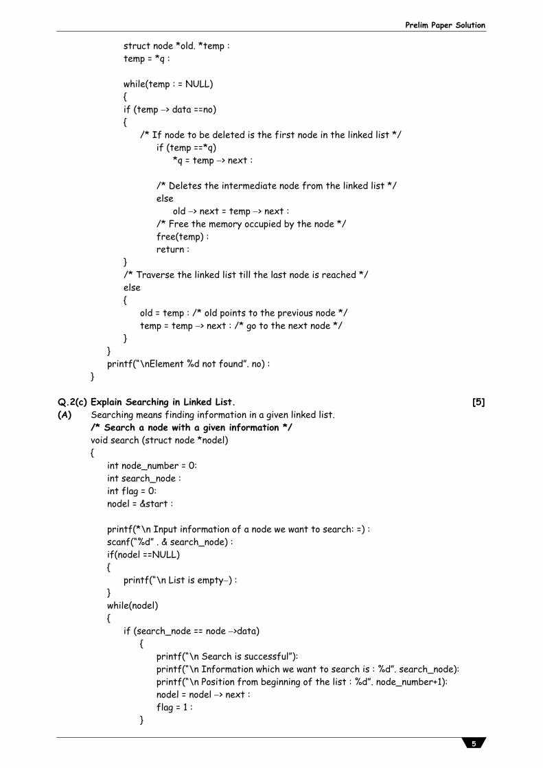
Q.3(b) Explain deque. [5](A) A deque is a linear list in which elements can be added or removed at either end but not in

the middle. The items can be added or deleted from the front or rear end, but no changes can be made elsewhere in the list.

There are two variations of a deque and input restricted deque and an output restricted

deque which are intermediate between deque and a regular queue. Specifically, an input restricted deque is a deque which allows insertions at only one end of the list, but allows deletions at both ends of the list. An output restricted deque which allows deletions at only one end of the list but allows insertions at both ends of the list.

Vidyalankar : S.Y. B.Sc. (IT) DS

10

The two possibilities that must be considered while inserting or deleting elements into the queue are :

When an attempt is also to insert an element into a deque which is already full, an overflow occurs.

When an attempt is made to delete an element from a deque which is empty, underflow occurs.

Q.3(c) Explain conversion of infix to postfix. [5](A) Rules :

1) If the operand is encountered, display it (or store it in result). 2) If the operator is encountered and the stack is empty then push it on the stack. 3) If operator is encountered and the stack is not empty then compare the entering

operator with residing operator (the current top of the stack). (a) If the entering operator has higher precedence than the residing operator then

push it on the stack (b) If the entering operator has lower or equal precedence than the residing operator

then the stack is popped and elements are displayed till either the residing operator’s precedence becomes higher or the stack becomes empty. Then the entering operator is pushed on to the stack.

(c) In case of brackets, the opening bracket has highest priority as a entering operator but the lowest priority as residing operator. Hence whenever opening bracket is encountered it is pushed on to the stack (Highest Priority). If the residing operator is opening bracket then any operator is pushed on the stack (Lowest Priority).

(d) Whenever the closing bracket is encountered, the stack is popped till the opening bracket is getting popped and all the popped elements are displayed. Both the closing and opening brackets are discarded.

In-fix to Post-fix Implementation: The program will used stack of char type int isoperand (char ch) { if (ch = ‘+’ || ch = = ‘’ || ch = = ‘*’ || ch = = ‘/’ || ch = = ‘%’) return 0; else return 1; } int ipr (char ch) int rpr (char ch) { { switch (ch) switch (ch) { { case ‘+’: case’+’: case ‘’: return 1; case ‘’: return 1; case ‘*’: case ‘*’: case ‘/’: case ‘/’: return 1; case ‘%”: return 2; case ‘%’: return 2; case ‘c’: return 0; case ‘(‘: return 0; return 1; } } } }

Fig.: Representation of a Deque

Prelim Paper Solution

11

void main ( ) { stack a; char in [50], post [50]; int l, i, k = 0, ele; a.tos = 1; printf (“Enter infix string in”); gets (in); l = strlen (in); for (i = 0; i < d; i ++) { if (in [i] = = ‘ (‘) push if (in [i] = = ‘)’) } while (isempty (&a)) { ele = pop (&a); if (ele = = ‘ (‘); break; post [ k + +] = ele; } } else if (is operand (in [i]) post [k++] = in [i]; else if (isempty (&a)) push (k a, in [i]); else if (ipr (in [i]) > rpr (stacktop (&a))) push (& a, in [i]); else { while (isempty (&a) = = 0&& ipr (in [i] < = rpr (stack to (&a))) { ele = pop (&a); post [k + +] = elc; { push (&a, in [i]); } } inside (isempty (&a) = = 0) { ele = pop (&a); post [k++] = ele; } post [k] = ‘/0’; printf (“postfix = %s”, post); }

Q.3(d) Explain priority queues. [5](A) Priority Queues : A queue in which we are able to insert items or remove items from any

position based on some property (such as priority of the task to be processed) is often referred to as a priority queue. Figure (a) represents a priority queue of jobs waiting to use a computer. Priorities of 1, 2 and 3 have been attached to jobs of type real-time, on-line, and batch, respectively. Therefore, if a job is initiated with priority i, it is inserted immediately at the end of the list of other jobs with priority i, for

Vidyalankar : S.Y. B.Sc. (IT) DS

12

i = 1, 2 or 3. In this example, jobs are always removed from the front of the queue. (In general, this is not a necessary restriction on a priority queue.) A priority queue can be conceptualized as a series of queue representing situations in which it is known a priori what priorities are associated with queue items. Figure (b) shows how the single-priority queue can be visualized as three separate queue, each exhibiting a strictly FIFO behavior. Elements in the second queue are removed only when the first queue is empty, and elements from the third queue are removed only when the first and second queues are empty. This separation of a single-priority queue into a series of queues also suggests an efficient storage representation of a priority queue. When elements are inserted, they are always added at the end of one of the queues as determined by the priority. Alternatively, if a single sequential storage structure is used for the priority queue, then insertion may mean that the new element must be placed in the middle of the structure. Task identification

R1 R2 … Ri-1 O1 O2 … Oi1 B1 B2 … Bk1 … 1 1 … 1 2 2 … 2 3 4 … 3 …

Priority ↑ ↑ ↑ Ri Rj Rk

(a) : A priority queue viewed as a single queue with insertion allowed at any position.

Priority 1 R1 R2 … Ri1 … ← Ri

Priority 2 O1 O2 … Oi1 … ← Oj

Priority 3 B1 B2 … Bk1 … ← Bk

(b) : A priority queue viewed as a setoff queue. Q.3(e) Explain implementation of circular queue. [5](A) Circular Queue If define CAP 5 typedef struct { int q [CAT], f, r, Flag; } queue; void insert (queue *t, int ele) {

if (t f = = 0 && t r = = cap 1 || t f = = t r + 1 & t flag = = 1) { printf (“Queue overflow”); returns; } t flag = 1; t r = (t r + 1)% CAP; t q [t r] = ele; } int isempty (queue *t)

Prelim Paper Solution

13

{ if (tflag = = 0) return 1; else return 0; } int delete1 (queue *t) { int z; if [isempty (t)] { print (“Queue underflow”); return 1; } if (t r = = t F) Flag = 0; z = t q [ t f] t F = (t f + 1) % CAP; return z; } int queuefront (queue *t) { if (isempty (t)) { printf (“queue Empty”); return 1; } return (t q [t f)); } void display (queue ++) { int i; if (isempty (t)) { printf (“Queue Empty”); return; } i = t f; while (1) { printf(“% f”, t q[i]); if (i = = t r) break; i = (i + 1)% CAP; } print [“\n”]; } Q.3(f) Explain application of queues. [5](A) It is the use of one system to imitate the behavior of another system. Simulations are

often used when it would be too expensive or dangerous to experiment with the real system. There are physical simulations, such as wind tunnels used to experiment with designs for car bodies and flight simulators used to train airline pilots. Mathematical simulations are systems of equations used to describe some system, and computer simulations use the steps of a program to imitate the behavior of the system under study.

Vidyalankar : S.Y. B.Sc. (IT) DS

14

In a computer simulation, the objects being studied are usually represented as data, often as data structures like structures or arrays whose entries describe the properties of the objects. Actions in the system being studied are represented as operations on the data, and the rules describing these actions are translated into computer algorithms. By changing the values of the data or by modifying these algorithms, we can observe the changes in the computer simulation, and then, we hope, we can draw worthwhile inferences concerning the behavior of the actual system in which we are interested. While one object in a system is involved in some action, other objects and actions will often need to be kept waiting. Hence, queues are important data structures for use in computer simulations. We shall study one of the most common and useful kinds of computer simulations, one that concentrates on queues as its basic data structure. These simulations imitate the behavior of systems (often, in fact, called queuing systems) in which there are queue of objects waiting to be served by various processes).

Q.4 Attempt the following (any THREE) [15]Q.4(a) Explain what are binary trees. Explain turns related to binary trees. [5](A) A tree is a collection of data stored in a hierarchical manner using different levels. A tree

starts from root and then it descends till the last level where all leaves are situated.

For better understanding, lets make some concepts clear using the following definitions. 1) Tree : It is a finite set of elements which can either be empty or can have distinguished

node ‘r’ called root with zero or more sub trees each of whose roots are connected to ‘r’ by edge.

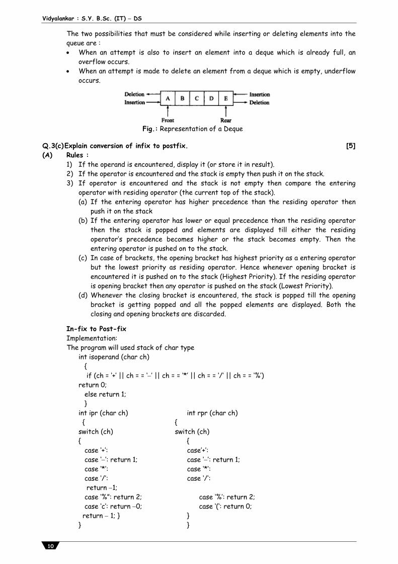
2) Binary Tree : It is a finite set of elements that can either be empty or can be divided into three subsets. The first subset contains a single element called root of the tree and the other two subsets themselves are binary trees called left and right sub tree of the original tree.

OR It is a tree in which each node can have at the most two children.

3) Node : Each element of a tree is called node, 4) Root : It is the distinguished node from which the tree originates. 5) Path : A path from node n1 to nk is defined as sequence of nodes n1, n2, … nk such that ni

is the parent of ni+1 for i =1 to k. - Length of the path is number of edges on the path. - In a tree there is exactly one path from the root to each node.

A

B D C

E F

G H I

J

A

B C

D E F G

Prelim Paper Solution

15

6) Depth of a node : For any node ni, the depth of ni is the length of the unique path from the root to ni.

- root is at depth 0. 7) Depth of the tree : Depth of the tree is equal to depth of the deepest leaf. 8) Height of a node : Height of a node ni is the longest path from ni to a leaf. - all leaves are at height 0 - nodes at same level may not have same height. 9) Height of the tree : The height of the tree is equal to the height of root. 10) Degree of a node : Degree of a node is the number of sub trees of the node.

- a node with degree 0 is called leaf node. 11) Degree of a tree : Degree of a tree is the degree of its node having maximum degree. 12) Ancestors of a node : All nodes on a path from root to a node are called ancestors of

that node. 13) Descendents of a node : All nodes having a path from the given nodes are called

descendents of that node. 14) Sub tree : It is defined as a tree formed using collection of some nodes and edges that are

present in original tree. 15) Forest : It is a collection of one or more disjoint trees.

Q.4(b) Explain Huffmann algorithm. [5](A) Huffman Algorithm

A binary tree is very useful in Huffman algorithm. Huffman Algorithm is useful in encoding and decoding messages. It gives efficient codes for each character in message depending on its frequencies. So that a character with highest frequency gets smallest code and vice versa. Suppose we have a message ACBDACA. If we keep two digit codes for every symbol as

A 00 B 01 C 10 D 11

Then there are total 7 symbols hence the complete message will require 2 * 7 = 14 bits. For the same message we can construct a Huffman Tree as follows.

The method of deriving codes for each symbol is to climb up till the root starting from the symbol. If climbed form left then 0 is added into code and if climbed from right then 1 is added to the code. Hence now codes for individual symbols can be derived as follows:

A 0 B 110 C 10 D 111

ACBD

A 3

CBD 4

C,2 BD,2

B,1 D,1

Vidyalankar : S.Y. B.Sc. (IT) DS

16

Then if calculated now the same message will require 11 bits. As the message length increases there would be significant reduction in number of bits.

Let us try to devise an algorithm for generating symbols using Huffman's Algorithm. Terms Used n Number of symbols frequency array storing frequencies of symbols code array storing codes of symbols position array which stores the position of symbols (address) rootnodes ascending priority queue

/* Initialize the set of root nodes */ root nodes = empty ascending priority queue /* constructing node for each symbol */ for (i=0; i<n; i++) { p = maketree (frequency[i]); position [i] = p; pqinsert ( rootnodes, p); } while (rootnodes contains more than one element) { p1 = pqmindelete (rootnodes); p2 = pqmindelete (rootnodes); /* combining p1 and p2 branches of single tree */ p = maketree (info (p1) + info (p2)); setleft (p,p1); setright (p,p2); pqinsert (rootnodes, p); } /* constructing tree and finding codes */ root = pqmindelete (rootnodes); // symbol with minimum frequency will be root for (i = 0; i < n; i++0) p = position [i]; initialize code[i[ to null string while (p ! = root) { /* travel up the tree i.e. climbing */ if (isleft (p) = = TRUE) code [i] = code[i] preceded by 0 (zero) else code [i] = code[i] preceded by 1 p=father (p); } /* end of while */ } /* end of for */

Prelim Paper Solution

17

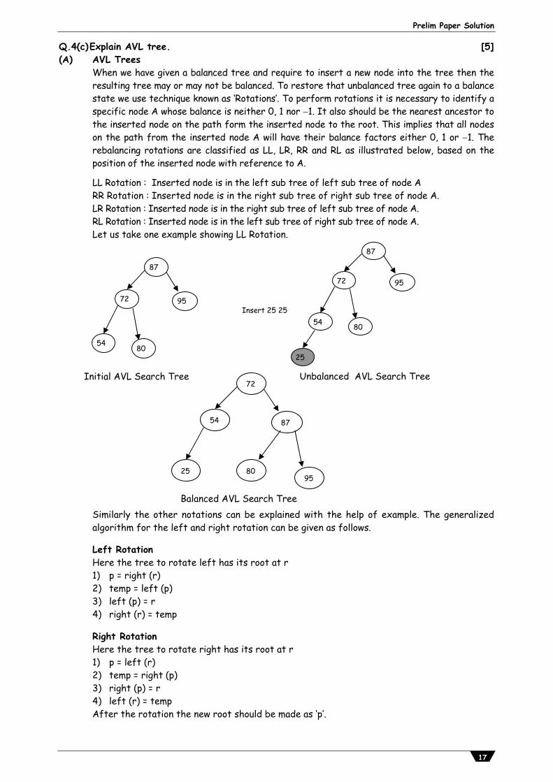
Q.4(c) Explain AVL tree. [5](A) AVL Trees

When we have given a balanced tree and require to insert a new node into the tree then the resulting tree may or may not be balanced. To restore that unbalanced tree again to a balance state we use technique known as ‘Rotations’. To perform rotations it is necessary to identify a specific node A whose balance is neither 0, 1 nor 1. It also should be the nearest ancestor to the inserted node on the path form the inserted node to the root. This implies that all nodes on the path from the inserted node A will have their balance factors either 0, 1 or 1. The rebalancing rotations are classified as LL, LR, RR and RL as illustrated below, based on the position of the inserted node with reference to A.

LL Rotation : Inserted node is in the left sub tree of left sub tree of node A RR Rotation : Inserted node is in the right sub tree of right sub tree of node A. LR Rotation : Inserted node is in the right sub tree of left sub tree of node A. RL Rotation : Inserted node is in the left sub tree of right sub tree of node A. Let us take one example showing LL Rotation.

Similarly the other notations can be explained with the help of example. The generalized algorithm for the left and right rotation can be given as follows.

Left Rotation Here the tree to rotate left has its root at r 1) p = right (r) 2) temp = left (p) 3) left (p) = r 4) right (r) = temp

Right Rotation Here the tree to rotate right has its root at r 1) p = left (r) 2) temp = right (p) 3) right (p) = r 4) left (r) = temp After the rotation the new root should be made as ‘p’.

Initial AVL Search Tree Unbalanced AVL Search Tree

87

72 95

80 54

87

72 95

80 54 Insert 25 25

25

72

54 87

80 25

Balanced AVL Search Tree

95

Vidyalankar : S.Y. B.Sc. (IT) DS

18

AVL tree (Adelson velskil and landis tree) AVL tree is Balanced Binary Search tree. In which every node must satisfy following criteria :

| h −hr | 1 h = height of left subtree hr = height of Right subtree.

If any node does not obey the criteria then the tree is unbalanced. AVL gives 4 Rotation Algorithm for 4 different cases, which are useful for Balancing the tree. Case 1 : Left − Left Case

100 is not balanced due to left−left case. So rotate 100 to right. This is Right rotation. Case 2 : Right − Right case

100 is not balanced due to right−right case. So rotate 100 to left. This is left rotation. Case 3 : Left − Right case

100 is not balanced due to left-right case. So rotate left child of 100. i.e. so this is left rotation. Case 4 : Right − Left case

100 is not balanced due to right-left case. So rotate right child of 100. i.e. 150 this is right rotation.

100 root

50

25

100

50

75

75

50 100

100

75

50

Left − left case

150

100 200

100

200

150

100

150

200

100 root

20

30

root

20

100 30

Prelim Paper Solution

19

Show the steps of creating AVL tree using following data . 1) 2)

3) 5)

4)

Improve Binary search tree searching become faster

6)

Root 2 is not Balanced due to Rightright, rotate left.

7)

Show the result of inserting 2 1 4 5 9 3 6 7 into an initially empty AVL tree.

1) 2)

3) 4)

2

4

5

1

6

3

4

5

6

2

7

1 3

4

6

7

2

3 1 5

2

1

2

1 4

2

1 4

5

2

3

4

1

2 root

root 1

2

1

2

1 3

5

4

2

1 4

5 3

4

5

6

2

3 1

1

2

3

Vidyalankar : S.Y. B.Sc. (IT) DS

20

5)

6)

2 is not balance because of 5, so right left

7)

5 is unbalanced rotate to the left Q.4(d) Explain insertion sort. [5](A) Insertion sort :

Algorithm 1) Create array of a[0 … n-1] of n elements. 2) initialize i to 0 3) initialize num to the element at i+1 4) for j = i downto 0 do the following a) if element at j is greater than num then shift the element at j to j+1 otherwise come out of the block 5) place num at j+1 6) increment i by 1 7) if i<n-1 then goto step 3 8) return the sorted array

2

5

9

1

4

3

2

4

5

1

9

3

4

5

9

2

3 1

4

5

9

2

3 1

6

Right left 4

5

6

2

9

3 1

4

6

9

2

3 1 5

7

2

1 5

9 4

2

5

9

1 4

Prelim Paper Solution

21

Analysis : Best Case : Even though the array is already sorted, one comparison is required in each pass. So 1 comparison for each pass and there are n passes which accounts to total of n-1 comparisons. Hence insertion sort gives best case efficiency of O(n).

Worst Case : It would be when array is sorted in the reversed order. Number of comparisons = (n-1) + (n-2) + ….. + 2 + 1 = n(n-1) /2 = n2 So it gives worst case efficiency of O(n2). Insertion sort is efficient when array is almost sorted.

Sample Output : Initial Array :

7 54 29 41 12 5 78 35 22 18

7 54 29 41 12 5 78 35 22 18

7 29 54 41 12 5 78 35 22 18

7 29 41 54 12 5 78 35 22 18

7 12 29 41 54 5 78 35 22 18

5 7 12 29 41 54 78 35 22 18

5 7 12 29 41 54 78 35 22 18

5 7 12 29 35 41 54 78 22 18

5 7 12 22 29 35 41 54 78 18

5 7 12 18 22 29 35 41 54 78

Q.4(e) Explain merge sort with an example. [5](A) Merge Sort

Algorithm : 1) Create array a[0 … n-1] of n elements. 2) Consider size equal to unity. 3) Subdivide the array in sub-arrays of ‘size’. 4) Merge these sub arrays in pairs of two such that they remain sorted. 5) Double the size. 6) if size <= array size then goto step 3 7) Return the sorted array.

Analysis : Here if the size of the input is n then the number of passes required is m such that n = 2m. Hence log n = m. So number of passes are m = log n.

Maximum number of comparisons made in each pass is n. Hence total comparisons can be calculated as follows: Total comparisons = Comparisons in each pass * No. of passes = n * m = n* log n

Hence the worst case complexity of Merge Sort is O(nlogn). Here the space complexity is not good. This sort gives very good time efficiency but requires extra space other than the array of input elements. The array ‘temp’ which of the same size as the input array is used while sorting. Generally a sorting technique which does not use extra space other than the set of input array, is known as ‘In place Sorting’ technique. Merge Sort is not ‘In Place Sorting’ technique. Sample Output : Initial Array :

7 54 29 41 12 5 78 35 22 18

7 54 29 41 5 12 35 78 18 22

7 29 41 54 5 12 35 78 18 22

5 7 12 29 35 41 54 78 18 22

Vidyalankar : S.Y. B.Sc. (IT) DS

22

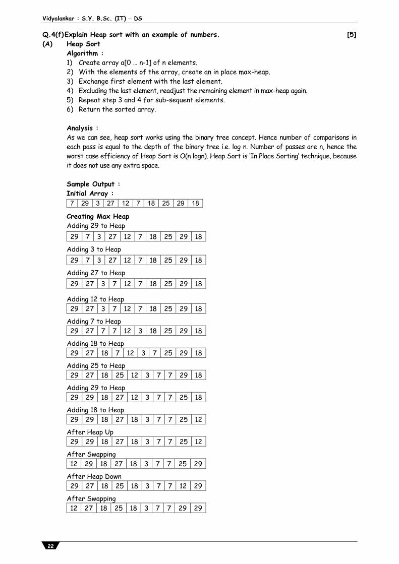
Q.4(f) Explain Heap sort with an example of numbers. [5](A) Heap Sort

Algorithm : 1) Create array a[0 … n-1] of n elements. 2) With the elements of the array, create an in place max-heap. 3) Exchange first element with the last element. 4) Excluding the last element, readjust the remaining element in max-heap again. 5) Repeat step 3 and 4 for sub-sequent elements. 6) Return the sorted array. Analysis : As we can see, heap sort works using the binary tree concept. Hence number of comparisons in each pass is equal to the depth of the binary tree i.e. log n. Number of passes are n, hence the worst case efficiency of Heap Sort is O(n logn). Heap Sort is ‘In Place Sorting’ technique, because it does not use any extra space. Sample Output : Initial Array : 7 29 3 27 12 7 18 25 29 18

Creating Max Heap Adding 29 to Heap 29 7 3 27 12 7 18 25 29 18

Adding 3 to Heap 29 7 3 27 12 7 18 25 29 18

Adding 27 to Heap 29 27 3 7 12 7 18 25 29 18

Adding 12 to Heap 29 27 3 7 12 7 18 25 29 18

Adding 7 to Heap 29 27 7 7 12 3 18 25 29 18

Adding 18 to Heap 29 27 18 7 12 3 7 25 29 18

Adding 25 to Heap 29 27 18 25 12 3 7 7 29 18

Adding 29 to Heap 29 29 18 27 12 3 7 7 25 18

Adding 18 to Heap 29 29 18 27 18 3 7 7 25 12

After Heap Up 29 29 18 27 18 3 7 7 25 12

After Swapping 12 29 18 27 18 3 7 7 25 29

After Heap Down 29 27 18 25 18 3 7 7 12 29

After Swapping 12 27 18 25 18 3 7 7 29 29

Prelim Paper Solution

23

After Heap Down 27 25 18 12 18 3 7 7 29 29

After Swapping 7 25 18 12 18 3 7 27 29 29

After Heap Down 25 18 18 12 7 3 7 27 29 29

After Swapping 7 18 18 12 7 3 25 27 29 29

After Heap Down 18 18 7 12 7 3 25 27 29 29

After Swapping 3 18 7 12 7 18 25 27 29 29

After Heap Down 18 12 7 3 7 18 25 27 29 29

After Swapping 7 12 7 3 18 18 25 27 29 29

After Heap Down 12 7 7 3 18 18 25 27 29 29

After Swapping 3 7 7 12 18 18 25 27 29 29

After Heap Down 7 7 3 12 18 18 25 27 29 29

After Swapping 3 7 7 12 18 18 25 27 29 29

After Heap Down 7 3 7 12 18 18 25 27 29 29

After Swapping 3 7 7 12 18 18 25 27 29 29

After Heap Down 3 7 7 12 18 18 25 27 29 29

Sorted Array 3 7 7 12 18 18 25 27 29 29

Q.5 Attempt the following (any THREE) [15]Q.5(a) Explain graph and methods to represent a graph. [5](A) Graph Representations

1) Adjacency Matrix : Let G = (V, E) be a graph of n vertices such that n >=1. Then adjacency matrix of G is a two-dimensional array of n x n say A where A[i][j] = 1 if edge (Vi, Vj) is present in E(G) A[i][j] = 0 if edge (Vi, Vj) is absent in E(G).

The graph shown in figure can be represented by, V(G) = {1,2,3,4} E(G) = { (1,4), (4,1), (2,3). (3,2), (2,4), (4,2), (3,4), (4,3) }

1

2 4

3

Vidyalankar : S.Y. B.Sc. (IT) DS

24

The same graph can be represented using Adjacency matrix as follows: Adj = 0 0 0 0

0 0 1 1 0 1 0 1 0 1 1 1

Adjacency matrix is also known as ‘Bit Matrix’ as it stores the presence and absence of the edge with the help of bits i.e. 1 for present and 0 for absent. Now if Adj is the adjacency matrix and Adj[i][j=1 then there exists a path between Vi and Vj. Adj2 = Adj * Adj (Boolean Matrix Multiplication) Now if Adj[i][j] =1 then it shows that there exists a path between Vi and Vj of length 2. Similarly we can have Adj3 = Adj2 * Adj ……. Adjn = Adj(n-1) * Adj.

2) Adjacency List Representation : As we have seen earlier that Adjacency matrix representation gives complexity of O(n2). It is because even though fewer edges are present still the traversal can not be completed till all the n2 elements are traversed. If the matrix is sparse i.e. not many edges are present then the earlier representation will result in huge amount of wastage of space. In such case, we can use the second type of representation for graph known as ‘Adjacency List Representation’. With this the performance can be improved to O(e+n) where n is number of vertices and e is number of edges. In adjacency list representation, n rows of matrix are represented by ‘n’ liked list. Each linked list stores the nodes adjacent to it. Every node will have two fields namely vertex and link.

The class can be defined as follows : class Node {

private int vertex; private Node link; }

The graph in the figure can be represented as follows:

1 4 2 3 3 2 4 4 1 3

Q.5(b) Explain BFS (Breadth first search). [5](A) Starting at vertex v and making it as visited, BFS visits next all unvisited vertices adjacent to v.

then unvisited vertices adjacent to there vertices are visited and so on. Algorithm : A breadth first search of G is carried out beginning at vertex v as bfs (v). All vertices visited are marked as visited [i]=true. The graph G and arrat visited are global and visited is initialized to false. Initialize, addqueue, emptyqueue, deletequeue are the functions to handle operations on queue.

1

2 4

3

Prelim Paper Solution

25

bfs (v) initialize queue q visited [v] = true addqueue(q,v) while not emptyqueue for all vertices w adjacent to v do if not visited [w] then addqueue (q,w) visited [w]=true deletequeue

Q.5(c) Explain depth first search. [5](A) The procedure of performing DFS on an undirected graph can be as follows : The starting vertex v is visited. Next an unvisited vertex w adjacent to v is selected and a

depth first search from w is initiated. When a vertex u is reached such that all its adjacent vertices have been visited, we back up to the last vertex visited which has an unvisited vertex w adjacent to it and initiate a depth first search from w. the search terminates when no unvisited vertex can be reached from any of the visited ones.

Algorithm : Given an undirected graph G=(V,E) with n vertices and an array visited[n]

initially set to false, this algorithm, dfs (v) visits all vertices reachable from v. Visited is a global array.

dfs (v) visited [v] = true for each vertex w adjacent to v if not visited [w] then dfs(w) Q.5(d) Explain Linear probing. [5](A) Suppose, that a new record R with key K is to be added into memory

table T. but that the memory location with hash addresses H(K) = h is already occupied. One natural way to resolve the collision is to assign R to the first available location. This collision resolution is called linear probing.

Linear probing is easy to implement but it suffers from “primary clustering”. A collision at any particular address in the memory indicates that many keys are mapped to the same address. Therefore, all keys mapped at that particular address will be clustered around the slot building up of long run of occupied slots. This would increase the search and insertion time values.

Q.5(f) Explain collision resolution techniques. [5](A) Every hash function is likely to generate the same address for some set different key

values. Suppose we want to add new records R with key K to our file F but suppose the memory location H(K) is already occupied. This situation is called collision. Therefore, one must know how to deal with such situations. The collision resolution techniques fall in two broad classes :

Open addressing Chaining