Embed Size (px)
Citation preview

SWEDISH SCHOOL OF ECONOMICS AND BUSINESS ADMINISTRATION
THE YRJÖ JAHNSSON WORKING PAPER SERIES
IN INDUSTRIAL ECONOMICS
6 (2004)
Oz Shy & Rune Stenbacka
SERVICE HOURS WITH ASYMMETRIC DISTRIBUTIONS OF IDEAL SERVICE TIME
2004

Service Hours With Asymmetric Distributions of Ideal Service Time Key words: Service Hours, Service Hour Competition, Nonuniform distribution of ideal service time JEL Classification: L81, M2, J51 © Swedish School of Economics and Business Administration, Oz Shy & Rune Stenbacka Oz Shy & Rune Stenbacka Swedish School of Economics and Business Administration P.O.Box 479 00101 Helsinki, Finland Distributor: Library Swedish School of Economics and Business Administration P.O.Box 479 00101 Helsinki Finland Phone: +358-9-431 33 376, +358-9-431 33 265 Fax: +358-9-431 33 425 E-mail: [email protected] http://www.hanken.fi/hanken/eng/page1579.php SHS intressebyrå IB (Oy Casa Security Ab), Helsingfors 2004 ISBN 951-555-858-1 ISSN 0424-7256

Service Hours With Asymmetric Distributions ofIdeal Service Time∗
Oz Shy†
University of Haifa, andSwedish School of Economics, and
WZ–Berlin
Rune Stenbacka‡
Swedish School of Economicsand HECER
October 13, 2004
Abstract
We show that private provision of service hours will be inefficiently low from a socialpoint of view independently of the market structure. We study how asymmetric distributionsof ideal service time impact on this market failure. We establish that the time gap betweenany two opening and closing hours in an oligopoly equilibrium is constant and that this timegap increases if the distribution of ideal service times becomes more uniform. Finally, weestablish that longest available service hours are sensitive to price changes but are invariantto changes in the market structure alone.
Keywords: Service Hours, Service Hour Competition, Nonuniform distribution of idealservice time
JEL Classification Numbers: L81, M2, J51
(Draft = hoursmonop45.tex 2004/10/13 10:39)
∗We are thankful for constructive comments from Paul Dobson, Staffan Ringbom and Michael Waterson.Financial support from The Yrjo Jahnsson Foundation and The Hanken Foundation is gratefully acknowledged.Part of this research was conducted while Rune Stenbacka was visiting WZB, whose hospitality is gratefullyacknowledged.
†WZB – Social Science Research Center Berlin, Reichpietschufer 50, D–10785 Berlin, Germany.E-mail: [email protected]
‡Department of Economics, Swedish School of Economics, P.O. Box 479, 00101 Helsinki, Finland.E-mail: [email protected]

1. Introduction
The performance of many industries, in particular all the service industries, is importantly affected
by the determination of service hours. Short service hours typically save costs for service operators,
but short business hours hurt consumers, who may face disutility associated with having to
advance or postpone their business transactions relative to their ideal time. Business hours have
always constituted a central issue that generates public debates no matter whether we focus on
private industries or industries with heavy public involvement. For example, in the private retailing
industry, business hours have traditionally been severely regulated in many European countries
and more recently the effects of business hour liberalization have generated heated debates in
the political arena as well as in the academic literature (see, for example, Clemenz (1990, 1994),
Kay and Morris (1987), Inderst and Irmen (forthcoming), Tangay, Vallee and Lanoie (1995) and
Thum and Weichenrieder (1997)). Similarly, no matter whether the transportation services in
metropolitan areas are outsourced to private operators or not, the local policymakers have to
determine the service hours and frequency of service.
In general, the determination of service hours is affected by at least four major considerations:
(a) There are typically important spillovers between periods. This means that some consumers
may advance (postpone) their service acquisition to the previous (next) period if the service is not
available at their ideal time. (b) There is typically an asymmetric distribution of consumers’ ideal
service time, which leads to regular fluctuations between phases of high demand and low demand
within each period. (c) The technology for service provision may exhibit increasing, constant or
decreasing returns to scale in both sales and service hours. Finally, (d) price competition may
be influenced by service hours. The novelty of our present approach is the focus on the first two
aspects by assuming that the consumers’ ideal service time follows an asymmetric distribution
on the unit circle. In particular, we explore the relationship between market structure, service
hour competition, and social welfare for a class of asymmetric distributions of ideal service time.
Further, we will focus on service hour provision in isolation from its possible implications for price
competition, because those issues have recently been analyzed by Inderst and Irmen (forthcoming)
1

as well as Shy and Stenbacka (2004) within the context of duopolistic retail industries for a given
unchanging distribution. In particular, in the present paper we explicitly explore the relationship
among classes of ideal service time distributions, market structure, service hour competition, and
social welfare.
Our analysis initially focuses on a private single operator. We characterize how the single
operator’s service hour provision depends on the degree of asymmetry of the distribution of
consumers’ ideal service time. We demonstrate that the private service provider will maintain
inefficiently short service hours from a social point view. Subsequently, we introduce competition
with respect to service hour provision.
For a duopolistic industry we characterize two feasible equilibrium configurations. First we find
that the duopoly equilibrium, where the providers maintain symmetric service hours around the
peak, has the feature that the service providers maintain different opening hours: One operator
opens earlier and closes later than its rival. Such an asymmetric equilibrium emerges because
there is a high return to a service operator from extending the hours relative to the rival, because
such an operator can automatically capture all those consumers who postpone or advance their
service acquisition. For such an equilibrium configuration we find that an increased degree of
uniformity of the distribution of ideal service times induces an increased degree of differentiation
with respect to the service hours. In this equilibrium configuration the service hour provision
by the operator providing long service hours is shown to coincide with the service hours offered
by a monopoly. We also characterize an alternative equilibrium configuration with service hours
asymmetrically around the peak. These two equilibrium configurations are found to be equivalent
from the social point of view.
Finally, we investigate an oligopoly industry of service operators. We establish that in the
oligopoly equilibrium the time gap between any two opening and closing hours is constant. Fur-
ther, we prove that this time gap increases if the distribution of ideal service times becomes more
uniform. Then, we conclude that the maximal service hours offered by the operator with the
longest opening hours is invariant to the market structure of service operators. This invariance
result implies that the social benefit of competition is realized at the price dimension and possibly
2

at the variety dimension, but not at the dimension represented by the longest available service
hours.
We are not aware of any existing research contribution, which analyzes the socially optimal
service hours, or the relationship between market structure and service hour provision, from the
point of view of a public economics perspective. There are some related studies of asymmetric
distributions of consumers’ ideal variety within the field of industrial economics. Neven (1986)
has explored some consequences for location equilibria of a non-uniform distribution of consumers
within the framework of a Hotelling model of horizontal product differentiation. Also, Waterson
(1990) has explored the consequences of asymmetries in the costs of supplying customers at
different points of the tastes spectrum, for the profitability of an oligopolistic industry within the
framework of horizontal product differentiation.
The present study is organized as follows. Section 2 develops a model of consumers who
differ in their ideal service time. Section 3 analyzes the profit-maximizing service hours of a single
service operator. Section 4 solves for the socially optimal service hours. Section 5 extends the
model to two competiting service providers. Section 6 extends the model to any arbitrary number
of service operators competing with respect to service hours. Section 7 explores some features
associated with a price equilibrium. Finally, Section 8 offers concluding comments.
2. The Model
Consider a single service provider, for example a store, operating in a given area (the “firm” in
what follows). What we have in mind here is a firm that provides a service, or sells a good, such
that consumers attach utility to the precise time at which the service is provided or delivered.
This means that the consumers’ utility is affected by a store’s opening hours, a bank’s service
hours and so on. Clearly, it seems that all services belong to this category. Our model also
fits more regulated industries, such as local bus companies with a decreased service of operation
during late night hours.
Time is indexed continuously on the unit circle. The unit circle representation is important
3
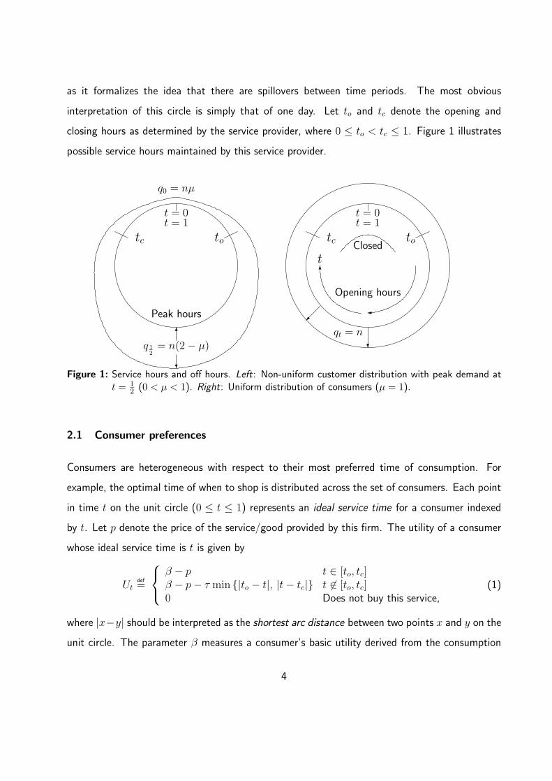
as it formalizes the idea that there are spillovers between time periods. The most obvious
interpretation of this circle is simply that of one day. Let to and tc denote the opening and
closing hours as determined by the service provider, where 0 ≤ to < tc ≤ 1. Figure 1 illustrates
possible service hours maintained by this service provider.
to totc tc
t = 0t = 1
t = 0t = 1
Peak hours �
�
Opening hours
t
q0 = nµ
q 12
= n(2 − µ)�
�
�qt = n
�
Closed
Figure 1: Service hours and off hours. Left: Non-uniform customer distribution with peak demand att = 1
2 (0 < µ < 1). Right: Uniform distribution of consumers (µ = 1).
2.1 Consumer preferences
Consumers are heterogeneous with respect to their most preferred time of consumption. For
example, the optimal time of when to shop is distributed across the set of consumers. Each point
in time t on the unit circle (0 ≤ t ≤ 1) represents an ideal service time for a consumer indexed
by t. Let p denote the price of the service/good provided by this firm. The utility of a consumer
whose ideal service time is t is given by
Utdef=
β − p t ∈ [to, tc]β − p − τ min {|to − t|, |t − tc|} t �∈ [to, tc]0 Does not buy this service,
(1)
where |x−y| should be interpreted as the shortest arc distance between two points x and y on the
unit circle. The parameter β measures a consumer’s basic utility derived from the consumption
4

of the service. The parameter τ > 0, which we refer to as the value-of-time parameter, measures
the per-unit-of-time disutility experienced by consumers when they are forced to either advance
or postpone their service acquisition, because the service is not offered at their ideal time. We
assume that the consumers are equally flexible when it comes to advancing or postponing the
acquisition of this service. Observe that when the ideal for the service falls outside of the service
hours, the consumer has two options: Either to postpone buying until service is resumed at to,
or to advance buying to the closing time tc.
In order to be able to distinguish between consumers who obtain service at their ideal time, and
those who do not, let to, where to < to, denote a consumer who is indifferent between postponing
purchasing the service to to, and not purchasing it at all. Similarly, let tc, where tc > tc, denote a
consumer who is indifferent between advancing purchasing the service to the closing hour tc and
not buying at all. Figure 2 illustrates the types of consumers who obtain service at their ideal
time, as well as consumers who must either postpone or advance their purchase.
totc
Postpone purchaseAdvance purchase
Do not purchase
Purchase at their ideal time
totc
t = 0t = 1
�
�
Opening hours
Figure 2: Consumers who obtain service at their ideal time, consumers with delayed or advanced service,and those who are not served at all.
2.2 Consumer distribution
In this paper, we wish to compute the service hours under a variety of asymmetric customer
distributions, which include peak and off-peak phases. For this reason, we will analyze a general
5

class of distribution functions in which the number of consumers with an ideal service time t is
qtdef=
{n[µ + 4(1 − µ)t] for ideal time 0 ≤ t ≤ 1
2
n[4 − 3µ − 4(1 − µ)t] for ideal time 12 < t < 1,
(2)
where 0 ≤ µ ≤ 1, measures the degree of uniformity. More precisely, if µ = 1 then qt = n for all
t, meaning that each time is an ideal service time for an equal number, n, of customers. That
is, µ = 1 implies that the distribution of ideal service time is uniform. Figure 1(left) illustrates
a non-uniform distribution with a peak at t = 12 , and off-peak at t = 0. As µ increases, the
distribution becomes more uniform as illustrated in Figure 1(right). In contrast, as µ declines
towards zero, the number of customers with an ideal service time at t = 0 vanishes, whereas the
number of peak customers at t = 12 is maximized reaching the level of q 1
2= 2n.
In a technical sense, the main justification for focusing on the distribution function (2) is that
it represents a “pure” shift in the degree of asymmetry, since any change in µ is independent
of the population parameter n. More precisely, the total number of buyers (ideal service time)
during the time intervals [0, 12 ] and [12 , 1] is constant and is given by
12∫
0
qt dt = n
12∫
0
[µ + 4(1 − µ)t] dt =
1∫12
qt dt = n
1∫12
[4 − 3µ − 4(1 − µ)t] dt =n
2. (3)
Furthermore, through the introduction of the parameter µ in (2), we are formally able to char-
acterize how asymmetries in the distribution of the consumers’ ideal service time affect the
endogenously-determined service hours.
We will make use of the following assumption.
Assumption 1
Consumers value their time. Formally,
τ >4(1 − µ)2 − µ
(β − p).
Assumption 1 can be easily interpreted by looking at extreme distributions. If µ = 1 (uniform
distribution), Assumption 1 becomes τ > 0. If µ = 0, this condition becomes τ/2 > (β − p),
6

which must be assumed in order to avoid the trivial solution where the store is open only for
a short time around t = 12 while serving the entire consumer population. If Assumption 1 is
reversed, consumers whose ideal time of service is half-a-day later or earlier would be willing to
wait or advance their service time. For these consumers, the cost of waiting or advancing would
be τ/2 whereas the benefit from obtaining the service would be (β − p).
Next, we will be using the following terminology.
Definition 1
We say that consumers are inflexible if they have a high value of time, formally if τ > 4(β − p).
We say that consumers are flexible if they have a low value of time, formally if
4(1 − µ)2 − µ
(β − p) < τ ≤ 4(β − p).
Intuitively, Definition 1 implies that if consumers have a high value of time, they will never advance
or postpone obtaining the service for more than 14 of a day as their benefit from the service β − p
is smaller than the time cost τ/4.
2.3 The service provider
The service provider controls two strategic instruments: The opening hour, to, and the closing
hour, tc. On the cost side, we assume that the service technology exhibits constant returns to
scale with a constant marginal cost c. In addition, we assume that the cost of operating the
business is w per unit of time. Therefore, the total cost of operation (independently of the sales
level) is w(tc − to). We will refer to w as the per-unit of time cost of business operation.
3. Equilibrium Service Hours of a Single Service operator
The environment discussed in the previous section extends Salop (1979) in the sense that it
allows for a non-uniform distribution of consumer tastes. However, we found out that closed
form solutions with respect to service hours and prices are impossible to obtain for a general
class of asymmetric distributions of ideal service times. For this reason we confine our analysis
7

to a fixed price p.1 Clearly, whenever we treat p as fixed, we must assume that β ≥ p ≥ c, so
that the price does not exceed consumers’ willingness to pay, and is not below the marginal cost.
Section 7 points out the difficulties of solving for price equilibria.
Figure 1(left) plots the consumer distribution defined in (2) and demonstrates that the off-
peak hours are symmetrically distributed around t = 0. Hence, a profit-maximizing service
provider would choose its service hours to satisfy tc = 1 − to. The utility function (1) implies
that the consumer indifferent between postponing the service deal or not buying at all, indexed
by to, is determined by the equation 0 = β − p − τ(to − to). Similarly, the location, tc, denoting
the consumer indifferent between advancing and not buying at all, is determined by 0 = β − p −τ(tc − tc). Therefore,
to = to − β − p
τand tc = tc +
β − p
τ. (4)
Clearly, a higher basic valuation parameter β decreases to and increases tc, hence increases
consumer participation. In contrast, an increase in the service price p increases the range of
excluded consumers.
Next, since the distribution of ideal service time (2) is symmetric around t = 12 , we will be
solving for an equilibrium where
to = 1 − tc and to = 1 − tc. (5)
This implies that the length of the service hours, when the service is offered, is tc − to = 1 − 2to.
Hence, Figure 2 and (5) imply that total output, which equals the total number of buyers, is
Q(to, tc) = n
12∫
to
[µ + 4(1 − µ)t] dt + n
tc∫12
[4 − 3µ − 4(1 − µ)t] dt = 2n
12∫
to
[µ + 4(1 − µ)t] dt, (6)
in a symmetric equilibrium where to = 1 − tc.1Stenbacka and Tombak (1995) made a similar assumption in their analysis of time-based competition, i.e.
competition based on service speed, within the framework of a vertical differentiation model, which exhibitscongestion effects.
8

Substituting (4) into (6) yields the number of served consumers as a function of the opening
hour only. Hence,
Q(to) = n
{1 − 2
(β − τto − p
τ
) [µ − 2(1 − µ)
(β − τto − p
τ
)]}. (7)
Thus, the number of excluded consumers is
n − Q(to) = n
{2(
β − τto − p
τ
) [µ − 2(1 − µ)
(β − τto − p
τ
)]}. (8)
Next, the cost of maintaining tc − to hours of operation is w(tc − to) = w(1 − 2to), again by
symmetry. Altogether, the service provider takes the price p as given, and chooses an opening
hour to to solve
maxto
π = (p − c)Q(t0) − w(1 − 2to), (9)
where Q is given in (7). Maximizing (9) with the respect to the opening hour to yields
to = 1 − tc =n(p − c) [4(1 − µ)(β − p) − µτ ] + wτ
4nτ(1 − µ)(p − c). (10)
We can show that
to ≤ 12
if w ≤ w|to= 12
def=1τ
n(p − c) [(2 − µ)τ − 4(1 − µ)(β − p)] . (11)
That is, the operating cost parameter must be below a certain level, specified in (11), to ensure
that the store is not always closed (the case where t0 = 12). Observe that Assumption 1 implies
that w|to= 12
> 0. Also, note that the second-order condition for a maximum is d2π/dt2o =
8n(1 − µ)(c − p) < 0 as the price was assumed to exceed marginal cost.
Next, by substituting the opening hour (10) into (4), we find that the buyers who are indifferent
between postponing their service to the opening hour to and not consuming at all, are indexed by
to = 1 − tc =w − nµ(p − c)
4n(p − c)(1 − µ)≥ 0 if w ≥ w|to=0
def= nµ(p − c). (12)
Otherwise, if w < nµ(p − c), to = 1 − tc = 0 meaning that all consumers are served. Notice
that w < nµ(p − c) implies that it is profitable to operate even the most off-peak time period
when consumer density is at its lowest level and is given by µn (see Figure 2). This condition
9

is interesting since to = 1 − tc = 0 does not mean that the service provider must operate at
t = 0. That is, the consumers located in the neighborhood of t = 0 can advance or postpone
their service time to the opening or closing hours.
Our comparative statics analysis will make sense only for interior equilibria where 0 < to <
to < 12 implying that some consumers are not served, and that the store is not always closed
(t < 12). To obtain these interior equilibrium configurations, (11) and (12) imply that the
operation cost parameter should be restricted as follows:
Assumption 2
The operating cost parameter is bounded from below and from above, so that the store is open
but not full time. Formally,
nµ(p − c) = w|to=0 < w < w|to= 12
=1τ
n(p − c) [(2 − µ)τ − 4(1 − µ)(β − p)] .
It is worth noting that when µ → 1, the range defined in Assumption 2 collapses to a singleton
where w = n(p − c). This means that under µ = 1 (uniform distribution), if w > n(p − c) the
store never opens, and if w < n(p − c) the store is open nonstop. In this respect the asymmetric
distribution of consumers is a crucial aspect of our model as the description of the optimal service
hours converges to such a trivial configuration in the limiting case of the uniform distribution.
To compute the equilibrium profit, substitute (10) into (9) for to to obtain
π =(2 − µ)2τn2(p − c)2 + 2nw[4(β − p)(1 − µ) − τ(2 − µ)](p − c) + w2τ
4nτ(1 − µ)(p − c). (13)
We now turn to analyzing how opening hours are affected by the parameters of the model.
Perhaps, the most interesting investigation is to alter the distribution of consumers’ ideal service
time, that is, changing the parameter µ in (2). We will make use of the following terminology.
Definition 2
We say that the operating cost, as reflected by the parameter w, is high relative to the operating
profit if w > wHM def= n(p − c); at a medium level if n(p − c)√
µ(2 − µ) def= wML ≤ w ≤ wHM .
Otherwise, if w < wML, we say that the operating cost is low.
10

Observe it is never profitable to provide service around the clock if the operating cost is high,
since the operating profit given by n(p − c) does not cover the cost of nonstop operation given
by 1 × w.
We now list the main findings of this section. Proofs are relegated to Appendix A.
Proposition 1
Suppose that the distribution of ideal service time (2) becomes more uniform (µ increases). Then,
(a) (i) Opening hours expand if the operating cost is not high.
Formally, dto/dµ < 0 whenever w < wHM .
(ii) Opening hours contract if the operating cost is high.
Formally, dto/dµ > 0 whenever w > wHM .
(b) The number of served consumers increases if and only if the operating cost is low.
More precisely,
dQ
dµ≥ 0 if and only if w ≤ wML = n(p − c)
√µ(2 − µ).
(c) Profit always declines. Formally, dπ/dµ < 0.
Part (c) is rather straightforward. To explain part (c) let us look at the opposite extreme situation
where all consumers have their ideal service time at t = 12 (i.e., a mass). Then, operation costs are
zero, whereas all consumers are served, hence profit reaches the highest possible level. Part (a)
shows that a more uniform distribution of ideal service time generates longer or shorter service
hours depending on whether the cost of operation is high or not. Intuitively, this result formalizes
the idea that the profit-maximizing service hours are extended when the distribution of customers
becomes more uniform if the cost of operation is below the high level, wHM. However, for very
high costs of operation the service hours are shortened, because in that case the firm has to
concentrate its operation so as to exploit the peak in demand and the opportunities for doing this
are reduced with a more uniform distribution of consumers. The result incorporated in part (b)
can be interpreted along similar lines with the qualification that it covers the number of served
customers instead of the service hours.
11

Figure 3 illustrates our Proposition 1.
�
n(p − c)√
µ(2 − µ)
�
All are servedRuled out by Ass.2
n(p − c)µ
w
wto= 12
No serviceRuled out by Ass.2
MediumLowwto=0 wML
Q ↑ to ↓ Q ↓ to ↓
‖ ‖
HighwHM
‖n(p − c)
Q ↓ to ↑
Figure 3: Illustration of Proposition 1: The effects of a more uniform distribution (µ ↑), as functions ofthe operation cost parameter w. Note: The range marked as High may be empty (Corollary 2).
The following corollary, proved in Appendix B, places a condition on buyers’ value of time
that is necessary to obtain the result listed in Proposition 1(a)(ii).
Corollary 2
A high value of time (see Definition 1) is a necessary condition for having a more uniform
distribution contracting the service hours.
It is instructive to summarize this section with a numerical example confirming the results
listed in Proposition 1. Table 1 displays some computations of the opening time t0, the marginal
customer type to, the number of served consumers Q, and the equilibrium profit π.
The upper part Table 1 clearly demonstrates that as µ increases, to increases (shorter service
hours), and compared with the lower two parts, this can happen only when the value of time is
high, as established in Corollary 2. Table 1 confirms that profit always declines when µ increases.
In addition, the Table confirms that the number of served customers Q declines for high values of
w and increases for low values of w. The two right columns demonstrate that the assumed values
of w indeed fall at the range of high, medium, and low operating costs as stated in Definition 2.
The column third from the right confirms that w falls in the range where the store maintains
some opening hours as defined by wto= 12
in (11).
12

High τ = 60 & High operating cost: w = 1250 > wHM
µ t0 t0 Q π wto= 12
wHM wML
0.4 0.467 0.276 61.45 656 1344 1200 9600.5 0.471 0.271 58.25 626 1320 1200 1039
Low τ = 40 & Medium operating cost: w = 1050 > wML
µ t0 t0 Q π wto= 12
wHM wHL
0.4 0.498 0.198 74.76 892 1056 1200 9600.5 0.487 0.187 74.22 864 1080 1200 1039
Low τ = 40 & Low operating cost: w = 900 < wML
µ t0 t0 Q π wto= 12
wHM wML
0.4 0.446 0.146 83.23 901 1056 1200 9600.5 0.425 0.125 84.37 877 1080 1200 1039
Table 1: Computer simulations demonstrating how the opening time, number of served customers, andprofit are affected when buyers’ distribution becomes more uniform (µ ↑). Simulations assumen = 100, β = 24, p = 12, and c = 0.
4. Socially Efficient Service Hours
This section computes the socially optimal opening and closing hours for our model. We then
compare these to the equilibrium service hours computed in the previous section.
We define the social welfare function of the economy as the sum of consumer surplus and
industry profit. Since prices are merely transfers from consumers to service providers, the social
welfare function is given by
W = 2(β − c)
12∫
to
qt dt − 2τ
t∗o∫to
qt(t∗o − t) dt − w(1 − 2t∗o), (14)
where qt is given in the upper part of (2). The first term measures buyers’ utility net of unit
production cost. The second term measures the total adjustment costs of the consumers who
have to advance or postpone their service acquisition so as the make transactions take place when
service is available. The last term is the cost of maintaining t∗c − t∗o = 1 − 2t∗o service hours.
Substituting (4) into (14) for to, and then differentiating with respect to t∗o shows that the
13

socially optimal opening hour is
t∗o =wτ − cn[4p(µ − 1) + 4β(1 − µ) − µτ ] − nβ[2β(µ − 1) + µτ ] − 2p2(µ − 1)
4nτ(1 − µ)(β − c). (15)
Subtracting the socially optimal opening hour from the equilibrium hour given in (10) yields
to − t∗o =(β − p)[2n(p − c)(1 − µ)(β − p) + wτ ]
4nτ(1 − µ)(p − c)(β − c)> 0. (16)
Hence,
Proposition 3
(a) A single service provider will maintain inefficiently short service hours from a social point of
view. Formally, to > t∗o and tc < t∗c .
(b) The provider’s profit-maximizing service hours equal the socially optimal level if the price is
set at the level where all consumer surplus is extracted. Formally, to = t∗o if p = β.
Part (a) can be intuitively explained by reference to the fact that the private service provider does
not internalize the social costs borne by those customers, who have to advance or postpone their
business transaction. In this respect, and at least in the absence of price effects, all regulation
which is designed to limit the service hours, seems to be misplaced as any potential economi-
cally justified regulation should impose requirements on minimum, not maximum, service hours.
Proposition 3(b) is very much related to Swan’s (1970a,b), where a price setting monopoly will
use the price system to extract more surplus, but will maintain social optimum with respect to
other decision variables (opening hours in the present case). Thus, a monopoly service provider
has an incentive to utilize only the price, and not service hours, to extract surplus from consumers.
We now ask what is the relationship between the magnitude of the market failure characterized
in Proposition 3 and the distribution of consumers’ ideal service time? By differentiation of (16)
with respect to µ, and separately with respect to the price p, we find that
d(to − t∗o)dµ
=w(β − p)
4n(p − c)(β − c)(1 − µ)2 > 0 and (17)
d(to − t∗o)dp
∣∣∣∣c=0
=−4np2(β − p)(1 − µ) − wβτ
4np2βτ(1 − µ)< 0.
14

Therefore, we can state the following proposition.
Proposition 4
The difference between the socially-optimal and the equilibrium opening hours
(a) increases when the distribution becomes more uniform, and
(b) decreases with an increase in the price of the service.
Thus, our model predicts that the market failure associated with reduced service hours is less
significant with a more asymmetric distribution of buyers’ ideal service time. The distortion is
magnified with a more uniform distribution of consumers. Intuitively this makes sense, because
with a more uniform distribution a larger number of consumers have to adjust the service time
of their business transaction.
Proposition 4(b) demonstrates that the shortage of service hours from a social viewpoint is
smaller for high-priced services (with insignificant marginal costs). This implies the following
corollary.
Corollary 5
In markets with low marginal service production cost, the introduction of price competition
enlarges the difference between the business hour equilibrium and the socially optimal service
hours.
The next section investigate whether competition in service hours (holding the price level
constant) can serve as a mechanism for extending the service hours towards the social optimum.
5. Equilibrium Service Hours under Duopoly
Suppose now that there are two service providers labeled as 1 and 2. Let t1o and t1c denote the
opening and closing time of service provider 1. t2o and t2c are similarly defined. We will distinguish
between two equilibrium configurations.
15

Definition 3
We say that a service operator i extends its opening hours symmetrically around the peak if
the time interval between the opening hour and the peak hour equals the time interval between
the peak hour and the closing hour. Formally, if 12 − tio = tic − 1
2 , i = 1, 2.
Section 5.1 analyzes symmetric service operations around the peak hour. Section 5.2 solves for
equilibria with service hours asymmetrically located around the demand peak.
5.1 Duopoly equilibrium with symmetric-around-the-peak service hours
Figure 4 displays opening and closing hours which are symmetric around the demand peak as-
suming, with no loss of generality, that t1o ≤ t2o and t1c ≥ t2c . Figure 4 shows that both firms
t2ot2c
Buy only 1Buy only 1
Do not purchase
Equally split between 1 & 2
t1ot1c
t = 0t = 1
�
�
Both open
t1ot1c
Postpone to t1oAdvance to t1c
Both closed
t = 12
Figure 4: Two service providers: Symmetric around the peak opening hours.
provide service between t2o and t2c . Firm 1 starts providing the service earlier, at t1o and closes at a
later time t1c . Therefore, given equal prices, all buyers indexed on [t1o, t1o) obtain the service later
than their ideal time, and from firm 1 only, whereas all buyers indexed on (t1c , t1c ] obtain their
service also from firm 1 and earlier than their ideal time.
16

Similar to (4), the buyers who are indifferent between obtaining the service at a non-ideal
time and not obtaining it at all are indexed by
t1o = t1o − β − p
τand t1c = t1c +
β − p
τ. (18)
In view of Figure 4, assuming that buyers split evenly between the providers when both stores
are open, the number of clients served by each firm is
q1 = 2n
t2o∫t1o
[µ+4(1−µ)t] dt+212n
12∫
t2o
[µ+4(1−µ)t] dt and q2 = 212n
12∫
t2o
[µ+4(1−µ)t] dt. (19)
The service providers choose the opening hours to solve
maxt1o
π1 = (p − c)q1 − w(1 − 2t1o) and maxt2o
π2 = (p − c)q2 − w(1 − 2t2o), (20)
where q1 and q2 are given in (19) and t1o in (18). It can be shown that d2π1/d(t1o)2 = 8n(1 −
µ)(c−p) < 0, and that d2π2/d(t2o)2 = 4n(1−µ)(c−p) < 0, hence both providers’ profit functions
are strictly concave with respect to their opening hours. Thus, the first-order conditions imply
the following opening hours:
t1o =n(p − c)[4(β − p)(1 − µ) − µτ ] + wτ
4nτ(1 − µ)(p − c)and t2o =
2w − µn(p − c)4n(1 − µ)(p − c)
. (21)
Comparing (21) with (10) demonstrates that the opening hour of firm 1 in duopoly competition
equals the opening hour of a single service provider. Thus, under duopoly, the service provider
who opens earlier determines the opening hour by equating the per-unit-of-time operating cost
w with the marginal operating profit at the opening hour. This consideration is identical to the
one made by a single provider, which is a consequence of our assumption that prices are fixed.
Why do two initially identical service providers end up maintaining different opening hours?
The answer is that the store that opens longer hours attains two additional market segments:
The early morning customers who postpone service to the opening hour, and late customers
who advance their service acquisition. In contrast, the store with shorter service hours captures
only customers at their ideal service times. Consequently, there is an additional return from
17

maintaining longer hours and this additional return explains why identical opening hours does
not constitute a Nash equilibrium. If the service provider with the shorter hours would match the
opening hours of the long hour operator, this additional return would be cut by half and would
not cover the additional operating costs.
The opening hours (21) imply that the difference between the two opening hours (hence, the
duration at which only one firm provides the service) is
t2o − t1o =wτ − 4n(1 − µ)(β − p)(p − c)
4nτ(1 − µ)(p − c)> 0 if w >
4n(1 − µ)(p − c)(β − p)τ
. (22)
Appendix C provides the proof of the following proposition.
Proposition 6
Suppose that (22) holds and that the distribution of ideal service time becomes more uniform (µ
increases). Then,
(a) Both providers extend their service hours if w < n(p − c)/2 = wHM/2.
(b) Provider 1 extends whereas provider 2 shortens business hours if n(p− c)/2 < w < n(p− c).
(c) Both providers shorten their service hours if w > wHM = n(p − c), that is if operating costs
are high according to Definition 2.
(d) The gap between the opening and closing hours of the two providers is enlarged.
The reader can notice the resemblance between Proposition 6 and Proposition 1 which is also
illustrated in Figure 3, as both firm 1 under duopoly competition, and a single provider offer
identical service hours, and hence react to changes in the distribution in the same way via the
parameter w. In fact, the condition listed in Proposition 6(a) and (b) can be logically deduced
since each provider serves 50% of the customers, hence the threshold value equals precisely to
wHM/2. For this reason we can omit a formal proof of this proposition. Part (d) means that an
increased degree of uniformity of the distribution of ideal service time implies an increased degree
of differentiation with respect to opening hours. This is a natural features because with a more
uniform distribution a larger number of consumers will adjust their business transactions to take
18

place during firm 1’s opening hours. This, in turn, will increase firm 1’s return from extended
service hours. At the same time, firm 2 will face a lower number of peak-hour customers, which
leads firm 2 to shorten its service hours.
Table 2 demonstrates our finding regarding the effect of a changing distribution on equilibrium
service hours.
Proposition 6(a): w = 550 < 600 = wHM/2µ t10 t10 t2o t2o − t1o π1 π2
0.2 0.080 0.173 0.224 0.051 326.62 146.300.3 0.056 0.149 0.220 0.071 323.06 131.490.4 0.024 0.117 0.215 0.099 323.31 116.74
Proposition 6(b): w = 650 > 600 = wHM/2µ t10 t10 t2o t2o − t1o π1 π2
0.2 0.107 0.199 0.276 0.077 326.33 96.300.3 0.086 0.179 0.280 0.101 327.23 81.490.4 0.059 0.151 0.285 0.133 333.44 66.74
Table 2: Computer simulations showing how the opening hours, difference in opening hours, numberof served customers, and profits are affected when buyers’ distribution becomes more uniform(µ ↑). Simulations assume n = 100, τ = 130, β = 24, p = 12, and c = 0.
Table 2 verifies and demonstrates the results listed in Proposition 6. The top table demon-
strates that the opening hours of firm 1 expand when operating expenses are sufficiently low.
The bottom table demonstrates that for intermediate operating costs provider 2 shortens its
service hours, whereas the large operator extends its service hours. Finally, Table 2 confirms
Proposition 6(d) showing that the gap between opening hours is enlarged with a more uniform
distribution.
We now wish to investigate how service hours are affected by an exogenous increase in the
price of the service. Differentiating (21) with respect to p yields
dt1odp
= − w
4n(1 − µ)(p − c)2 − 1τ
< 0 anddt2odp
= − w
2n(1 − µ)(p − c)2 < 0. (23)
Hence,
19

Proposition 7
Suppose that there is an increase in the price of the service, then
(a) Both service providers extend their service hours.
(b) The difference between the service hours of the two providers increases as long as the oper-
ating cost does not exceed a certain threshold level. Formally,
d (t2o − t1o)dp
≥ 0 if and only if w ≤ 4n(1 − µ)(p − c)2
τ.
The intuition behind the first part is straight forward as it is clear that a higher price makes it
more profitable to extend service hours. Part (b) states that firm 1 extends its hours “faster”
than firm 2 for sufficiently low operating costs, and vice versa.
5.2 Duopoly equilibrium with asymmetric-around-the-peak service hours
Figure 5 displays asymmetric opening and closing hours assuming, with no loss of generality, that
firm 1 opens earlier than firm 2 and also closes earlier than firm 2, that is t1o ≤ t2o and t1c ≤ t2c .
Comparing Figure 5 to Figure 4 reveals that both providers maintain the same opening hours.
The difference between the figures is that in Figure 5 provider 1’s closing time is earlier than that
of provider 2. However, in Figure 5 both providers maintain the same length of opening hours
(in contrast to Figure 4 where provider 1 maintains longer hours). Loosely speaking, Figure 5
“reverses’ the roles of provider 1 and provider 2 during the second half of the day.
Clearly, since in this asymmetric equilibrium both service operators provide the same lengths
of opening hours, they bear the same operation costs. Hence, there is no need to recalculate the
opening and closing hours. Instead, we need only switch between t1c and t2c , therefore,
t1c = 1 − t2o =n(p − c)(4 − 3µ) − 2w
4n(1 − µ)(p − c)and (24)
t2c = 1 − t1o =n(p − c)[τ(4 − 3µ) − 4(β − p)(1 − µ)] − wτ
4nτ(1 − µ)(p − c),
where t1o and t2o are given in (21). Now we can state the following proposition.
20

t2ot1c
Buy only 1Buy only 2
Do not purchase
Equally split between 1 & 2
t1ot2c
t = 0t = 1
�
�
Both open
t1ot2c
Postpone to t1oAdvance to t2c
Both closed
t = 12
Figure 5: Two service providers: Asymmetric around the peak opening hours.
Proposition 8
(a) There exist two equilibria where the service operators extend their opening hours asymmet-
rically around the peak. (b) In both equilibria, one service provider opens early and closes early,
whereas the competing provider opens late and closes late. (c) Both providers earn the same
profits.
The asymmetric configuration captured by Proposition 8 could be exemplified by the opening
hour pattern often applied by bars and night clubs. Night clubs tend to open late and close late.
It is important to emphasize that the symmetric and the asymmetric equilibrium configurations
generate allocations, which are equivalent from a social point of view as long as the prices are
fixed. Of course, in a more general context with endogenous prices it may matter a great deal
from a social point of view whether the equilibrium configuration is symmetric or asymmetric
around the peak. In such a generalized context, the asymmetric business hour configuration may
facilitate market sharing and thereby serve as a collusion device.
21

6. Equilibrium Service Hours under Oligopoly
Sections 3 and 5 analyzed the market structures with a single service provider as well as a duopoly.
In this section we demonstrate how our model can be extended to incorporate any number of
service providers. Perhaps the most interesting issue to investigate is the time gaps between the
providers’ opening (and closing) hours.
Suppose now that there are φ ≥ 3 service providers who all choose to be open around the
peak time t = 12 . As before, we assume that the buyers are equally divided among all operators
which are open. Figure 6 illustrates possible opening hours on the half-circle [0, 12 ].
Off-peak(t = 0)
Peak(t = 1
2)
t1o
t1o
t2ot3o
t4o t5o t6o
t7o
tφo
No providers
1 provider2 providers
3 providers 4 providers5 providers
6 providers
7 providers
φ providers
Figure 6: Equidistant opening hours under oligopoly.
Let f(µ, t) def= µ + 4(1 − µ)t. A straigtforward generalization of (19) shows that the number
of buyers served by firm i (for 2 ≤ i ≤ φ − 1) is
qi =2ni
ti+1o∫
tio
f(µ, t) dt +2n
i + 1
ti+2o∫
ti+1o
f(µ, t) dt + · · · +2nφ
12∫
tφo
f(µ, t) dt. (25)
That is, consumers with an ideal time close to t = 12 are divided among a larger number of
providers, whereas buyers whose ideal service time is further away from t = 12 are successively
divided among fewer providers. Similar to (20), each of the above service providers chooses the
opening hour tio to maximize πi = (p − c)qi − w(1 − 2tio), where qi is given in (25). Abstracting
from corner solutions, the opening hour of provider i is given by
tio =i w − µn(p − c)4n(1 − µ)(p − c)
. (26)
22

Since d2πi/d(tio)2 = 8n(1 − µ)(c − p) < 0, (26) is a unique maximum. Differentiating (26) with
respect to the distribution parameter µ and the price p yields
dtiodµ
=i w − n(p − c)
4n(p − c)(1 − µ)2 anddtiodp
=i w
4n(µ − 1)(p − c)2 , (27)
where the second expression is always negative. Therefore,
Proposition 9
(a) When the distribution becomes more uniform, service providers with longer service hours are
more likely to extend their opening hours than providers with shorter service hours. Formally,
dtiodµ
≤ 0 if and only if i ≤ n(p − c)w
.
(b) All service providers increase their service hours when the price increases.
Note that the firms indexed by a lower i have longer service hours. Part (a) implies that a low
value of the product i × w induces these firms to extend hours when the distribution becomes
more uniform. This holds true, because making the distribution more uniform shifts buyers from
firms indexed by a high i with concentrated service hours towards firms with longer service hours.
For this reason, part (a) captures the idea that firms indexed by high i tend to reduce their service
hours since they tend to lose buyers.
In order to gain further insights how opening and closing hours vary across oligopoly com-
petitors, let us look at a provider indexed by j < i. Then, (26) implies that
tio − tjo =w(i − j)
4n(1 − µ)(p − c). (28)
In particular, setting j = i + 1 yields the following proposition.
Proposition 10
(a) The time gap between any two opening and closing hours is constant. Formally, ti+1o − tio is
independent of i, for any service provider 2 ≤ i ≤ φ.
(b) The time gap between any two opening hours (similarly, between any two closing hours)
increases when the distribution becomes more uniform.
23

Part (a) confirms the configuration illustrated in Figure 6, which exhibits opening hours at con-
stant intervals. Of course, this result may be attributed to the assumption of the constant value
of time parameter, τ . The only exception is service provider 1 with the longest service hours. The
reason is that firm 1 also serves buyers whose ideal service time falls when no firm provide any
service. That is, firm 1 also serves buyers indexed on [t1o, t1o) and [t1c , t
1c ] during which no firm pro-
vides any service. Proposition 10(b) captures the idea that a service operator with longer business
hours has higher returns from extending its service hours further in response to a shift towards
more off-peak customers. In this sense, a shift towards a more uniform distribution of consumers
leads to a higher degree of business hour differentiation. Or, conversely, a change towards a more
asymmetric distribution of consumers induces a tendency towards increased agglomeration of the
service hours around the peak hour.
7. Service Hours and Pricing Decisions
Our analysis has so far assumed that the price of the service/good has been fixed. This could
be the result of a regulatory requirement, or some kind of resale price maintenance marketing
arrangements. In this section we “reverse” our assumption regarding the strategic decisions
by holding the opening and closing hours constant and characterizing the price equilibrium. In
particular, we are interested in finding out how the price equilibrium is affected by varying the
(now) exogenously-given service hours.
Substituting (7) into (9), and then maximizing (9) with respect to p, taking to as given, yields
p(to, µ) =√
A + B + C
6(1 − µ), where
Adef= 4c2(µ − 1)2 + 2c(µ − 1)(4toτ(µ − 1) + 4β(1 − µ) − µτ) + 4t2oτ
2(µ − 1)2
Bdef= 2toτ(1 − µ)(4β(µ − 1) + µτ) + 4β2(µ − 1)2 + 2βµτ(µ − 1) + τ 2(µ − 3µ + 3)
Cdef= 2c(1 − µ) + 4toτ(µ − 1) + 4β(1 − µ) − µτ.
(29)
From this algebraic expression, the reader can already observe that although closed-form solutions
for the price equilibrium and the associated profits can be obtained, systematic and general
24
comparative statics are hard to display. Therefore, we here extract only some limited observations
based on numerical simulations.
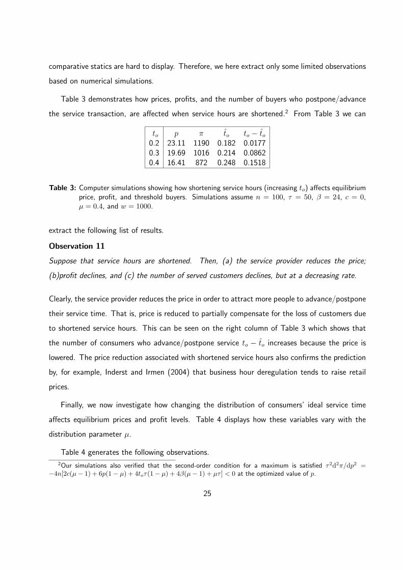
Table 3 demonstrates how prices, profits, and the number of buyers who postpone/advance
the service transaction, are affected when service hours are shortened.2 From Table 3 we can
to p π to to − to0.2 23.11 1190 0.182 0.01770.3 19.69 1016 0.214 0.08620.4 16.41 872 0.248 0.1518
Table 3: Computer simulations showing how shortening service hours (increasing to) affects equilibriumprice, profit, and threshold buyers. Simulations assume n = 100, τ = 50, β = 24, c = 0,µ = 0.4, and w = 1000.
extract the following list of results.
Observation 11
Suppose that service hours are shortened. Then, (a) the service provider reduces the price;
(b)profit declines, and (c) the number of served customers declines, but at a decreasing rate.
Clearly, the service provider reduces the price in order to attract more people to advance/postpone
their service time. That is, price is reduced to partially compensate for the loss of customers due
to shortened service hours. This can be seen on the right column of Table 3 which shows that
the number of consumers who advance/postpone service to − to increases because the price is
lowered. The price reduction associated with shortened service hours also confirms the prediction
by, for example, Inderst and Irmen (2004) that business hour deregulation tends to raise retail
prices.
Finally, we now investigate how changing the distribution of consumers’ ideal service time
affects equilibrium prices and profit levels. Table 4 displays how these variables vary with the
distribution parameter µ.
Table 4 generates the following observations.2Our simulations also verified that the second-order condition for a maximum is satisfied τ2d2π/dp2 =
−4n[2c(µ − 1) + 6p(1 − µ) + 4toτ(1 − µ) + 4β(µ − 1) + µτ ] < 0 at the optimized value of p.
25

µ p π to to − to0.4 19.69 1016 0.214 0.08610.5 19.35 969 0.207 0.09300.6 18.97 922 0.199 0.1006
Table 4: Computer simulations showing how making the distribution more uniform (increasing µ) affectsequilibrium price, profit, and threshold buyers. Simulations assume n = 100, τ = 50, β = 24,c = 0, to = 0.3, and w = 1000.
Observation 12
Suppose that buyers’ distribution of ideal service time becomes more uniform (µ increases). Then,
(a) equilibrium price and profit decrease; and (b) more consumers are served
The increase in the number of served consumers follows from two effects operating in the same
direction: The decline in p and the shift of consumers from peak to off-peak hours.
8. Conclusion
In this study we have theoretically established that private provision of service hours will be
inefficiently low from a social point of view independently of the market structure. We have
investigated how asymmetric distributions of ideal service time impact on this market failure.
We have shown that the time gap between any two opening and closing hours in an oligopoly
equilibrium is constant and that this time gap increases if the distribution of ideal service times
becomes more uniform. Finally, we have established that maximal service hour provision is
invariant to the market structure in the industry of service operators. This invariance result
means that the social benefit of competition is realized at the price dimension and possibly at the
variety dimension, but not at the dimension represented by the longest available service hours.
Appendix A. Proof of Proposition 1
Differentiating (10) and (12) with respect to µ yields
dtodµ
=dtodµ
=w − n(p − c)
4n< 0 if w < n(p − c) = wHM .
26

This proves part (a). To prove part (b), observe that
dQ
dµ=
µ(2 − µ)n2(p − c)2 − w2
4n(1 − µ)2(p − c)2 ≥ 0 if and only if w ≤ wML.
Finally, to prove (c),
dπ
dµ=
c2n2µ(µ − 2) − 2cn[npµ(µ − 2) + w] + n2p2µ(µ − 2) + 2npw − w2
4n(p − c)(1 − µ)2 < 0
if w > µn(p − c) which holds by Assumption 2.
Appendix B. Proof of Corollary 2
As shown in Figure 3, this case happens when w fall in the interval where wHM < w < w|t= 12.
(11) and Definition 2 imply that this interval is nonempty if τ > 4(β − p), which means high
value of time according to Definition 1.
Appendix C. Proof of Proposition 6
Part (c) is identical to Proposition 1(a). To prove (a), Differentiating (21) with respect to µ
yieldsdt2odµ
=2w − n(p − c)
4n(1 − µ)2(p − c)≤ 0 if w ≤ wHM
2.
Part (b) is implied by parts (a) and (c). To prove part (d), (22) implies that
d(t2o − t2o)dµ
=w
4n(1 − µ)2(p − c)> 0.
27

References
Clemenz, G. 1990. “Non-Sequential Consumer Search and the Consequences of a Deregulationof Trading Hours.” European Economic Review, 34: 1323–1337.
Clemenz, G. 1994. “Competition Via Shopping Hours: A Case for Regulation?” Journal ofInstitutional and Theoretical Economics, 150: 625–641.
Inderst, R., and A. Irmen. Forthcoming. “Shopping Hours and Price Competition.” EuropeanEconomic Review.
Kay, J., and C. Morris. 1987. “The Economic Efficiency of Sunday Trading Restrictions.”Journal of Industrial Economics, 36: 113–129.
Neven, D. 1986. “On Hotelling’s Competition with Non-Uniform Customer Distributions,”Economics Letters, 21: 121–126.
Salop, S. 1979. “Monopolistic Competition with Outside Goods.” Bell Journal of Economics,10: 141–156.
Shy, O., and R. Stenbacka. 2004. “Price Competition, Business Hours, and Shopping TimeFlexibility,” available for downloading from www.ozshy.com .
Stenbacka, R., and M. Tombak. 1995. “Time-Based Competition and the Privatization ofServices,” Journal of Industrial Economics, 43: 435–454.
Swan, p. 1970a. “Durability of Consumer Goods.” American Economic Review, 60: 884–894.
Swan, p. 1970b. “Market Structure and Technological Progress: The Influence of Monopolyon Product Innovation.” Quarterly Journal of Economics, 84: 627–638.
Tangay, G., L. Vallee and P. Lanoie. 1995. “Shopping Hours and Price Levels in the RetailingIndustry: A Theoretical and Empirical Analysis.” Economic Inquiry, 33: 516–524.
Thum, M., and A. Weichenrieder. 1997. “Dinkies and housewifes: The regulation of shoppinghours.” Kyklos, 50: 539–560.
Waterson, M. 1990. “Product Differentiation and Profitability: An Asymmetric Model,” Journalof Industrial Economics, 39: 113–130.
28

The Yrjö Jahnsson Working Paper Series in Industrial Economics is funded by The Yrjö Jahnsson Foundation. Editor of the Working Paper Series: Professor Rune Stenbacka 2001 1. Anthony Dukes & Esther Gal-Or: Negotiations and Exclusivity Contracts for
Advertising 2. Oz Shy & Rune Stenbacka: Partial Subcontracting, Monitoring Cost, and
Market Structure 3. Jukka Liikanen, Paul Stoneman & Otto Toivanen: Intergenerational Effects in the Diffusion
of New Technology: The Case of Mobile 2002 1. Thomas Gehrig & Rune Stenbacka: Introductory Offers in a Model of Strategic Competition 2. Amit Gayer & Oz Shy: Copyright Protection and Hardware Taxation 3. Christian Schultz: Transparency and Tacit Collusion in a Differentiated Market 4. Luis H. R. Alvarez & Rune Stenbacka: Strategic Adoption of Intermediate
Technologies: A Real Options Approach 5. Thomas Gehrig & Rune Stenbacka: Information Sharing in Banking:
An Anti-Competitive Device? 6. Oz Shy & Rune Stenbacka: Regulated Business Hours, Competition, and Labor Unions 7. Jean Jacques-Laffont, Scott Marcus, Patrick Rey & Jean Tirole:
Internet Interconnection and The Off-Net-Cost Pricing Principle 8. Marc Ivaldi & Frank Verboven: Quantifying the Effects from Horizontal Mergers in European
Competition Policy 9. Ari Hyytinen & Otto Toivanen: Do Financial Constraints Hold Back Innovation and
Growth? Evidence on the Role of Public Policy 10. Staffan Ringbom & Oz Shy: Advance Booking, Reservations and Refunds 2003 1. Luis H. R. Alvarez & Rune Stenbacka: Irreversibility, Uncertainty and Investment in the
Presence of Technological Progress 2. Thomas Gehrig & Rune Stenbacka: Screening Cycles 3. Thomas Gehrig & Rune Stenbacka: Differentiation-Induced Switching Costs and Poaching 4. Luis H.R. Alvarez & Rune Stenbacka: Outsourcing or In-house Production? A Real Options
Perspective on Optimal Organizational Mode 5. Staffan Ringbom & Oz Shy: Reservations, Refunds, and Price Competition 6. Joanne Sault, Otto Toivanen & Michael Waterson: Learning and Location 7. Tuomas Takalo & Otto Toivanen: Entrepreneurship and Financial Markets with Adverse
Selection 2004 1. Oz Shy & Rune Stenbacka : Liquidity Provision and Optimal Bank Regulation 2. Heikki Kauppi, Erkki Koskela & Rune Stenbacka: Equilibrium Unemployment and Investment Under Product and Labour Market Imperfections 3. Mikael Juselius: The Relationship Between Wages and the Capital-Labor Ratio: Finnish Evidence on the Production Function 4. Erkki Koskela & Rune Stenbacka Agency Cost of Debt and Credit Market Imperfections: a
Bargaining Approach 5. Luis H. R. Alvarez & Rune Stenbacka: Takeovers and Implementation Uncertainty: A Real
Options Approach 6. Oz Shy & Rune Stenbacka : Service Hours With Asymmetric Distributions of Ideal Service Time