Swarm and Evolutionary Computation 4 (2012) 44–53

Contents lists available at SciVerse ScienceDirect

Swarm and Evolutionary Computation

journal homepage: www.elsevier.com/locate/swevo

Regular paper

State estimation of nonlinear stochastic systems using a novel meta-heuristicparticle filterMohamadreza Ahmadi a, Hamed Mojallali a,∗, Roozbeh Izadi-Zamanabadi ba Electrical Engineering Department, Faculty of Engineering, University of Guilan, P.O. Box: 3756, Rasht, Iranb Department of Electronic Systems, Automation & Control, Aalborg University, Fredrik Bajers Vej 7, 9220, Aalborg Ø, Denmark

a r t i c l e i n f o

Article history:Received 19 April 2011Received in revised form26 September 2011Accepted 21 November 2011Available online 13 December 2011

Keywords:Particle filterSub-optimal filteringNonlinear state estimationInvasive weed optimization

a b s t r a c t

This paper proposes a new version of the particle filtering (PF) algorithm based on the invasive weedoptimization (IWO) method. The sub-optimality of the sampling step in the PF algorithm is prone toestimation errors. In order to avert such approximation errors, this paper suggests applying the IWOalgorithm by translating the sampling step into a nonlinear optimization problem. By introducing anappropriate fitness function, the optimization problem is properly treated. The validity of the proposedmethod is evaluated against three distinct examples: the stochastic volatility estimation problem infinance, the severely nonlinear waste water sludge treatment plant, and the benchmark target trackingon re-entry problem. By simulation analysis and evaluation, it is verified that applying the suggested IWOenhanced PF algorithm (PFIWO) would contribute to significant estimation performance improvements.

© 2011 Elsevier B.V. All rights reserved.

1. Introduction

State estimation plays a key role in different applications suchas fault detection, process monitoring, process optimization, andmodel based control techniques [1]. Fortunately, a large group ofmodels in signal processing can be represented by a state-spaceform inwhich prior knowledge of the system is available. This priorknowledge allows us to exploit a Bayesian estimation approach.Within this statistical framework, one can perform inference onthe unknown states according to the posterior distribution. Inmost cases, the observations arrive sequentially in time, and oneis interested in recursively estimating the hidden states from thetime-varying posterior distribution. This problem is referred asthe optimal filtering problem [2,3]. Owing to the mathematicalcomplexity, only few specific models (including linear Gaussianstate-space models and finite state-space hidden Markov models(HMM) [4]) can be adopted to reach an analytical solution. Thepopular Kalman filter (KF) [2,3] and the renowned HMM filter [4]provide close form solutions to the latter models.

In many real-life applications, however, the models possessnonlinearity and non-Gaussian behavior. Thus, an optimal solutionto the filtering problem cannot be attained. In this case, it becomesnecessary to exploit approximate and computationally traceable

∗ Corresponding author. Tel.: +98 131 6690276 8; fax: +98 131 6690271.E-mail addresses: mrezaahmadi@ieee.org (M. Ahmadi), mojallali@guilan.ac.ir

(H. Mojallali), riz@es.aau.dk (R. Izadi-Zamanabadi).

2210-6502/$ – see front matter© 2011 Elsevier B.V. All rights reserved.doi:10.1016/j.swevo.2011.11.004

sub-optimal solutions to the sequential Bayesian estimationmethodology. Over the past decades, several sub-optimal filteringmethods such as the extended Kalman filter (EKF), and theunscented Kalman filter (UKF) have been proposed in the openliterature [5]. But, these filtering algorithms suffer from the curseof dimensionality; that is, they perform poorly as the dimension ofthe model states increases. Furthermore, the rate of convergenceof the approximation error decreases dramatically for large statedimensions, say 4 [5]. Notably, it has been demonstrated thatthe estimation performance of UKF inhibits intrinsic limitations.In other words, the deterministic choice of the so called sigmapoints confines the flexibility desired to construct a probabilitydistribution.

The particle filter (PF), first brought forward byGordon et al. [6],employs a set of N random samples (or particles) to approximatethe posterior distribution. The particles are evolved over time viaa combination of importance sampling and re-sampling steps. Ina few words, the re-sampling step statistically multiplies and/ordiscards particles at each time step to adaptively concentrateparticles in the regions of high posterior probability [7]. Thepopularity of the PF results from the notion that it does not callfor model simplification or adopting special distributions.

Recently, researchers have shown an increased interest inthe subject of integrating meta-heuristic algorithms in PF. Ina seminal paper, Tong et al. [8] proposed an optimized PFbased on particle swarm optimization (PSO) algorithm [9] whichdemonstrated improved estimation accuracy. Many subsequentstudies also followed the same trend using PSO; e.g., refer

M. Ahmadi et al. / Swarm and Evolutionary Computation 4 (2012) 44–53 45

to [10,11]. In [10], the authors exploited a similar method basedon PSO for visual tracking, and claimed that the modified schemehas better accuracy than the conventional PF. Later, Jing et al. [11]further advanced the algorithm brought forward in [8] with anew re-sampling strategy. However, to authors’ knowledge, therehas been very little discussion on developing other meta-heuristicbased PF algorithms, thus far. The studies reported to date havefocused on adjusting the PSO enhanced PF algorithm rather thanincorporating other techniques established upon evolutionaryalgorithms and swarm intelligence.

The bio-inspired IWO algorithm was introduced by Mehrabianand Lucas [12] which imitates the colonial behavior of invasiveweeds in nature. The IWO algorithm has shown to be virtu-ous in converging to optimal solution by employing some basiccharacteristics of weed colonization, e.g. seeding, growth and com-petition. In [13], Chakraborty et al. investigated the search per-formance and specifically the effect of population variance on theexplorative power of the algorithm. Later, Roy et al. [14] proposeda hybrid optimization algorithm by integrating the optimal forag-ing theory in IWO which evinced improved optimization capac-ity. Previously, the IWO algorithm has been utilized in a surfeitof applications including optimizing and tuning of a robust con-troller [12], antenna configuration optimization [15], optimal ar-rangement of piezoelectric actuators on smart structures [16], DNAcomputing [17], and etc.

This paper considers the implementation of the IWO algorithmas a mean to optimize the PF method. Since sampling in PF iscarried out in a sub-optimal manner, it can bring about someperformance defects such as sample impoverishment [5]. Byintroducing a suitable fitness function for particles, such problemsare circumvented and an enhanced PF algorithm is achievedthanks to the IWO approach. The functionality of the combinedmethod is verified using three nonlinear state estimation problemsfrom different fields: volatility estimation of a stock market, stateestimation of a nonlinear chemical process, and the re-entryvehicle tracking problem.

The rest of this paper is organized as follows. Section 2 providesa concise description of some preliminary notions including thefiltering problem, the Monte Carlo method, Importance Sampling,and the basic particle filtering algorithm. The IWO algorithm islimned in Section 3. The proposed PFIWO method is discussed inSection 4. Simulation Results based on the PFIWO algorithm andsome discussions are outlined in Section 5. Section 6 concludes thepaper.

2. Preliminaries

2.1. The filtering problem

Consider the general class of nonlinear non-Gaussian systemswith state-space model as described below

xk = f (xk−1, uk−1, vk−1), xk ∼ p(xk|xk−1) (1a)

yk = g(xk, uk, wk), yk ∼ p(yk|xk), (1b)

where the subscript k denotes the time instance. xk ∈ Rnx representthe system states with probability distribution of p(xk|xk−1) whichis not directly measurable, and yk ∈ Rny is the noise corruptedobservation with likelihood p(yk|xk). The maps f ∈ Rnx × Rnu ×

Rnv → Rnx and g ∈ Rnx × Rnu × Rnw → Rny are generally nonlinearfunctions. u stands for known inputs. v andw represent the processand measurement noise, respectively. The overall structure isillustrated in Fig. 1. Filteringis the task of sequentially estimatingthe states (parameters or hidden variables) of a system as a setof observations become available on-line [2,3]. Strictly speaking,filtering is aimed at estimating the posterior distribution p(xk|yk)as a set of observations Yk = (y1, y2, . . . , yk)T arrives. It is worthnoting that the results obtained in this section are established upon

Fig. 1. A graphical representation of the state-space model described by Eq. (1).

Fig. 2. The Bayesian approach to the filtering problem.

the following assumptions:1. The states follow a first order Markov process, i.e., xk|xk−1 ∼

pxk|xk−1(xk|xk−1) with an initial distribution of p(x0).2. The measurements are conditionally independent given the

states, i.e., each yk only depends on xk.

The Bayesian solution to the filtering problem consists of twostages [2,3,5]:1. Prediction: let the above assumptions hold. Using the prior

density function, and the Chapman–Kolmogorov equation wehave

p(xk|yk−1) =

p(xk|xk−1)p(xk−1|yk−1)dxk−1. (2)

2. Correction: based on the Bayes’ formula

p(xk|yk) =p(yk|xk)p(xk|yk−1)

p(yk|yk−1)(3a)

wherein

p(yk|yk−1) =

p(yk|xk)p(xk|Yk−1)dxk. (3b)

The algorithm is initialized with p(x0|y0) = p(x0) and p(x1|y0) =

p(x1). One step operation of the Bayesian filtering is portrayed inFig. 2. However, it is obvious that achieving a closed form analyticalsolution to the untraceable integral in Eq. (2) and therefore thesolution to Eq. (3) is a cumbersome task. The problem becomeseven more severe as the state dimensions increase. Thus, anoptimal solution cannot be attained except under very restrictingconditions (linear transition functions and Gaussian noise) usingthe well-known KF. The interested reader can refer to [2,3] whichprovide a comprehensive theoretical overview of available optimalmethods. Sub-optimal solutions exist for rather general modelswith nonlinear evolution functions and non-Gaussian noises.Nevertheless, due to the nature of thesemethods (e.g. EKF andUKF)which are based on local linearization, the estimation performanceis, more or less, limited. Estimation techniques established uponsequential Monte Carlo methods, namely the PF, are a promisingalternative to local linearization algorithms [6,18].

2.2. Monte Carlo and importance sampling techniques

In theMonte Carlo technique, one is concernedwith estimatingthe properties of some highly complex probability distributionp(x), e.g. expectation

E(s(x)) =

s(x)p(x)dx (4)

where s(x) is some useful function for estimation. In cases wherethis cannot be obtained analytically, the approximation problemcan be handled indirectly. It is possible to represent p(x) by a set

46 M. Ahmadi et al. / Swarm and Evolutionary Computation 4 (2012) 44–53

of random samples xi, i = 1, 2, . . . ,N . Consequently, the MonteCarlo representation is [16]

p(x) =1N

Ni=1

δ(x − xi) (5)

where δ(.) is the Dirac delta function. Then, the expectation can bereformulated as:

E(s(x)) =

s(x)p(x)dx ≈

s(x)

1N

Ni=1

δ(x − xi)dx

=1N

Ni=1

s(xi). (6)

Alternatively, suppose that the samples xi are drawn from adistribution q(x) instead of p(x). Now, the expectation can beestimated using importance sampling as follows:

E(s(x)) =

s(x)p(x)dx =

s(x)

q(x)p(x)q(x)

dx

≈

s(x)

p(x)q(x)

1N

Ni=1

δ(x − xi)dx

=1N

Ni=1

s(xi)p(xi)q(xi)

=1N

Ni=1

wis(xi) (7)

where wi ∝p(xi)q(xi)

is the importance weight. So, p(x) can beestimated as

p(x) =

Ni=1

wiδ(x − xi), s.t.Ni=1

wi = 1. (8)

2.3. The basic particle filter

The particle filtering scheme approximates the multi-dimensional integral in the Bayesian prediction and update stepsusing Monte Carlo sampling. Consider Eqs. (2) and (3), the discus-sion is followed by reformulating the latter equations based on theMonte Carlo approximation described in the previous section. Letxi, i = 1, 2, . . . ,N be the drawn samples from the posterior dis-tribution p(xk|yk). The filter is initialized as [5,18,19]:

xj0 ∼ p(x0|y0), i = 1, 2, . . . ,N. (9)Then, for k = 1, 2, . . . we have

p(xk|yk) =

Ni=1

wki δ(x − xik), s.t.

Ni=1

wki = 1. (10)

For i = 1, 2, . . . ,N sample from the proposal distributionq(xk|xk−1) as

xjk ∼ q(xk|xjk−1). (11)

Subsequently, update the importance weights

wki = wk−1

ip(yk|xik−1)p(x

ik|x

ik−1)

q(yk|xik−1). (12)

Provided that p(xk|xk−1) = q(xk|xk−1), Eqs. (11) and (12) convertto

xjk ∼ p(xk|xjk−1) (13a)

wki = wk−1

i p(yk|xik−1). (13b)Then, for i = 1, 2, . . . ,N normalize the weights

wki =

wki

Nj=1

wkj

. (14)

A prevalent problem with PF is the degeneracy phenomenon,wherein after few iterations, all but few particles will have trivialweights. A measure of degeneracy is the effective sample size Neffwhich can be empirically evaluated as

Neff =1

Ni=1

(wki )

2

. (15)

The conventional approach to solve around the problem of sampledegeneracy is to define a degeneracy threshold Nth. If Neff < Nth,re-sampling should be initiated [7].

3. The invasive weed optimization

3.1. Key terms

Prior to describing the IWO algorithm, the key terms areexplained as follows:a Seed: each unit in the colony (here the particles) thatencompasses a value for each variable in the optimizationproblem before fitness evaluation.

b Weed/Plant: any seed that is evaluated grows to aweed or plant.c Fitness: a value corresponding to the goodness of each unit afterbeing evaluated.

d Field: the search/solution space.e Maximumweed population: a parameter preset representing themaximum number of possible weeds in the field after fitnessassessment.

3.2. The IWO algorithm

The process flow of the IWO algorithm is outlined below[14,15]:1. Initialize the seeds Si = (s1, s2, . . . , sn)T , where n is the number

of selected variables, over the search space. Thus, each seedcontains random values for each variable in the n − D solutionspace.

2. The fitness of each individual seed is calculated according tothe optimization problem, and the seeds grow to weeds ableto produce new units.

3. Each individual is ranked based on its fitness with respect toother weeds. Subsequently, each weed produces new seedsdepending on its rank in the population. The number of seeds tobe created by eachweed alters linearly fromNmin toNmax whichcan be computed using the equation given below

Number of seeds =Fi − Fworst

Fbest − Fworst(Nmax − Nmin) + Nmin. (16)

In which Fi is the fitness of i’th weed. Fworst, and Fbest denotethe best and the worst fitness in the weed population. This stepensures that each weed takes part in the reproduction process.

4. The generated seeds are normally distributed over the fieldwithzeromean and a varying standard deviation of σiter described by

σiter =

itermax − iter

itermax

n

(σ0 − σf ) + σf (17)

where itermax and iter are the maximum number of iterationcycles assigned by the user, and the current iteration number,respectively. σ0 and σf represent the pre-defined initial andfinal standard deviations. n is called the nonlinear modulationindex. In order to obtain a full and swift scan of possible valuesof standard deviation, it has been examined that the mostappropriate value for nonlinear modulation index is 3 [15].The fitness of each seed is calculated along with their parentsand the whole population is ranked. Those weeds with lessfitness are eliminated through competition and only a numberof weeds remain which are equal toMaximumWeed Population.

M. Ahmadi et al. / Swarm and Evolutionary Computation 4 (2012) 44–53 47

5. The procedure is repeated at step 2 until themaximum numberof iterations allowed by the user is reached.

4. The proposed PFIWO algorithm

At the outset of this section, some exclusive features of the IWOalgorithm are emphasized. The IWO algorithm certifies that allpossible candidates would participate in the reproduction process.In contrast, most meta-heuristic algorithms would not allow theless-fitted individuals to produce offspring such as the GA. Besides,the IWO algorithm is straightforward and it includes less deal ofcomputational burdenunlike othermethods. As a good illustration,one can consider the PSO algorithm. PSO needs to update both theposition and velocity of individuals in each iteration round whichrequire some extra calculations to find the best position in theneighborhood of each particle aswell as thewhole population. Thisissue imposes a considerable deal of computational burden.

Having reviewed a number of unique characteristics of IWO,the discussion is proceeded by presenting the proposed PFIWOalgorithm. Owing to the fact that the sampling step of theconventional PF is sub-optimal, the IWO is suggested as a meansto enhance the sampling step. Here, the goal of the IWO in thesampling step is to trace the particles which correspond to greaterweights. Therefore, it is convenient to calculate the fitness of i’thparticle as

Fi =p(yk|xik−1)p(x

ik|x

ik−1)

q(yk|xik−1)(18)

which in case of p(xk|xk−1) = q(xk|xk−1) reduces to

Fi = p(yk|xik−1). (19)Consequently, the IWO algorithm’s task would be to maximize thefitness function. The sampling step is modified as follows:1. The fitness of each particle is evaluated, and the particles are

ranked based on their fitness in the population; i.e., thoseparticles which correspond to greater weights are of higherrank.

2. Perform steps 3, 4, and 5 of the IWO algorithm as describedin Section 3 until a predefined number of iteration cycles isreached. It isworth noting that since the basic PF is considerablytime-consuming the maximum number of iteration cyclesshould be chosen as a compromise between estimationperformance and algorithm run-time.

3. Subsequently, the weights are updated and normalized usingEqs. (13) and (14).

4. In order to reproduce and pick out the particles with largerweights the re-sampling step is implemented. That is,

xik, w

ki

Ni=1 =

xik,

1N

N

i=1. (20)

5. Simulation results

In this section, the estimation performance of the proposedPFIWO method is examined and compared with the conventionalPF. Three examples are investigated in this section. The firstexample is devoted to stochastic volatility estimation of asimulated market. The second example considers the stateestimation problem of a highly nonlinear chemical process, wastewater sludge treatment. Lastly, the performance of both algorithmsis challenged with a target tracking on the re-entry problemwhich has been actively studied as a benchmark for comparing thefunctionality of several estimation methods.

5.1. The stochastic volatility problem

A prominent group of structures for analyzing volatility aremodels in which the variance is specified to follow some latent

Fig. 3. The fluctuations of the stock prices in the simulated market.

Table 1The parameter values regarding the simulated stock market.

µ φ σ ση S1

0.1 0.99 0.1 0.05 10000

stochastic processes. Such models are referred to as stochasticvolatility (SV) models which appear in the theoretical financeliterature on option pricing [20–24]. Practical translations of theSVmodel are classically formulated in discrete time. The canonicalmodel in this class for regularly spaced data is [20,24]

xt+1 = µ + φ(xt − µ) + σηηt t ≥ 2 (21a)

h1 ∼ N

µ,σ 2

1 − φ2

(21b)

yt = ext+µ

2

ξt t ≥ 1 (21c)

where superscript t accounts for discrete time in days, and xt is theunobserved log volatility. yt denotes the daily log return calculatedas

yt = log

StSt−1

(22)

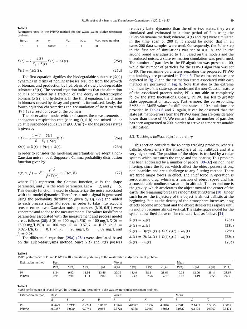
which is earned on stock S between days t and t − 1. ht is thelog volatility at day t which is assumed to follow a stationaryprocess (|φ| < 1). ξt and ηt are uncorrelated Gaussian processes(representing themarket shocks)with zeromean and variance of 1.φ is the persistence in the volatility, andση signifies the volatility ofthe log volatility. Regarding the economical aspects of the SVmodel,the interested reader can refer to [20]. Using Eqs. (21) and (22), thefinancial market corresponding to the parameters listed in Table 1was simulated. The fluctuations of stock prices are simulated for atime period of 500 days as depicted in Fig. 3. In the first 50 days,the prices grow as the market experiences desirable conditions.Fromday 51 on, due to say a financial crisis, the stock prices declinedramatically. The daily log return of stock prices is as sketched inFig. 4. The corresponding volatility is as illustrated in Fig. 5. The PFalgorithm as described in Section 2.3. was implemented with 80particles and the degeneracy threshold was chosen as Nth = 70.

One should note that the values for itermax,Nmax, andNmin mustbe selected such that the run-time of the algorithm do not exceedthe tolerable range. Moreover, it is important to notice that furtherincrementing the values for these parameters do not necessarilylead to better results. The initial and final dispersion standarddeviations (σ0 and σf ) should be adjusted such that the desirable

48 M. Ahmadi et al. / Swarm and Evolutionary Computation 4 (2012) 44–53

Fig. 4. Daily log return associated with the simulated stock market.

Fig. 5. Resultant stochastic volatility.

Table 2Parameters used in the PFIWO method for the stochastic volatility problem.

itermax σ0 σf Nmax Nmin Max. weed number

20 1 0.001 5 1 50

Table 3MAPE performance of PF and PFIWO in 10 simulations pertaining to the stochasticvolatility problem.

Estimation method Best (%) Worst (%) Mean (%)

PF 1.54 8.61 6.13PFIWO 0.78 3.39 1.89

Table 4RMSE performance of PF and PFIWO in 10 simulations pertaining to the stochasticvolatility problem.

Estimation method Best Worst Mean

PF 0.1892 2.3471 0.3943PFIWO 0.0627 0.8154 0.0836

estimation accuracy is reached in regard with itermax. All in all, thesuitable values of these parameters can be achieved empiricallydepending on the application.

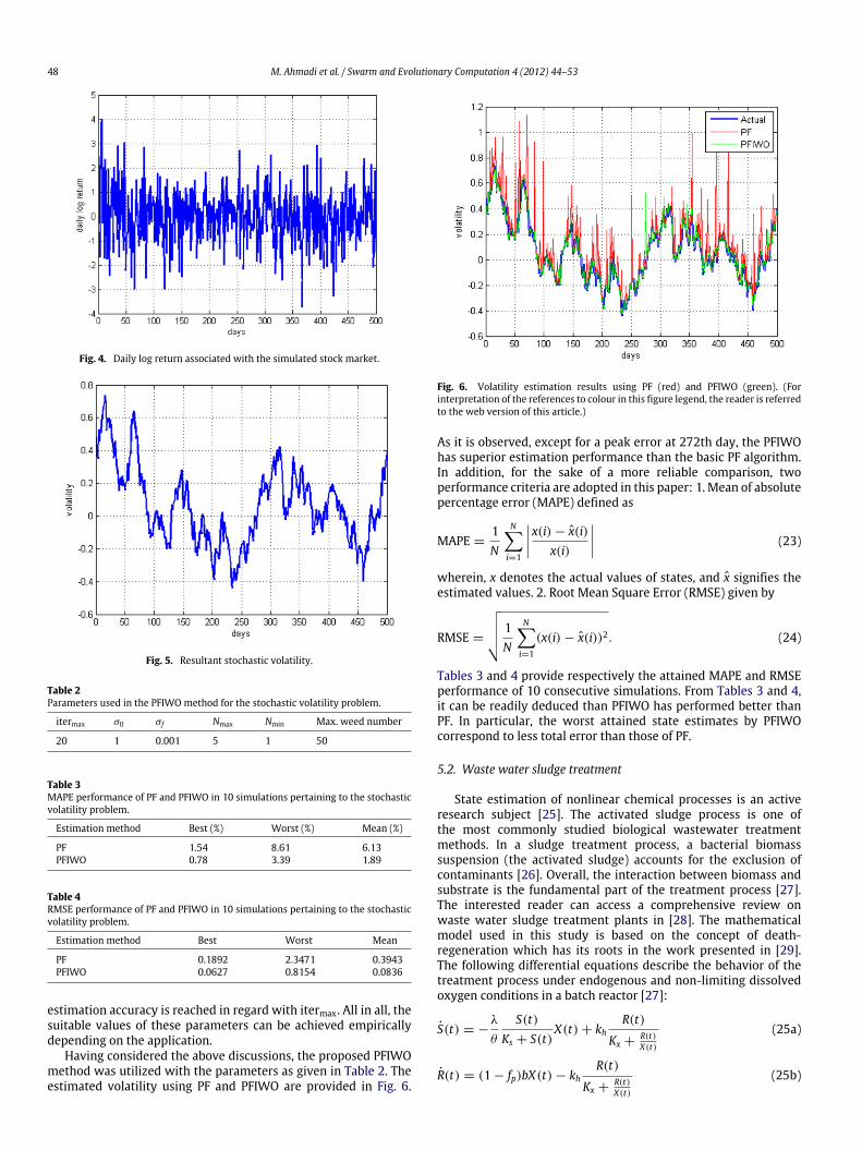
Having considered the above discussions, the proposed PFIWOmethod was utilized with the parameters as given in Table 2. Theestimated volatility using PF and PFIWO are provided in Fig. 6.

Fig. 6. Volatility estimation results using PF (red) and PFIWO (green). (Forinterpretation of the references to colour in this figure legend, the reader is referredto the web version of this article.)

As it is observed, except for a peak error at 272th day, the PFIWOhas superior estimation performance than the basic PF algorithm.In addition, for the sake of a more reliable comparison, twoperformance criteria are adopted in this paper: 1. Mean of absolutepercentage error (MAPE) defined as

MAPE =1N

Ni=1

x(i) − x(i)x(i)

(23)

wherein, x denotes the actual values of states, and x signifies theestimated values. 2. Root Mean Square Error (RMSE) given by

RMSE =

1N

Ni=1

(x(i) − x(i))2. (24)

Tables 3 and 4 provide respectively the attained MAPE and RMSEperformance of 10 consecutive simulations. From Tables 3 and 4,it can be readily deduced than PFIWO has performed better thanPF. In particular, the worst attained state estimates by PFIWOcorrespond to less total error than those of PF.

5.2. Waste water sludge treatment

State estimation of nonlinear chemical processes is an activeresearch subject [25]. The activated sludge process is one ofthe most commonly studied biological wastewater treatmentmethods. In a sludge treatment process, a bacterial biomasssuspension (the activated sludge) accounts for the exclusion ofcontaminants [26]. Overall, the interaction between biomass andsubstrate is the fundamental part of the treatment process [27].The interested reader can access a comprehensive review onwaste water sludge treatment plants in [28]. The mathematicalmodel used in this study is based on the concept of death-regeneration which has its roots in the work presented in [29].The following differential equations describe the behavior of thetreatment process under endogenous and non-limiting dissolvedoxygen conditions in a batch reactor [27]:

S(t) = −λ

θ

S(t)Ks + S(t)

X(t) + khR(t)

Kx +R(t)X(t)

(25a)

R(t) = (1 − fp)bX(t) − khR(t)

Kx +R(t)X(t)

(25b)

M. Ahmadi et al. / Swarm and Evolutionary Computation 4 (2012) 44–53 49

Table 5Parameters used in the PFIWO method for the waste water sludge treatmentproblem.

itermax σ0 σf Nmax Nmin Max. weed number

15 1 0.0001 3 1 80

X(t) = λS(t)

Ks + S(t)X(t) − bX(t) (25c)

P(t) = fpbX(t). (25d)

The first equation signifies the biodegradable substrate (S(t))dynamics in terms of nonlinear losses resulted from the growthof biomass and production by hydrolysis of slowly biodegradablesubstrate (R(t)). The second equation indicates that the alterationof R is controlled by a fraction of the decay of heterotrophicbiomass (X(t)) and hydrolysis. In the third equation, the changein biomass caused by decay and growth is formulated. Lastly, thefourth equation characterizes the accumulation of inert material(P(t)) as a result of decay of the biomass.

The observation model which subsumes the measurements –endogenous respiration rate (r in mg O2/l h) and mixed liquorvolatile suspended solids (Ω in gCOD/m3) – and the process statesis given by

r(t) = λ1 − θ

θ

S(t)Ks + S(t)

X(t) (26a)

Ω(t) = X(t) + P(t) + R(t). (26b)

In order to consider the modeling uncertainties, we adopt a non-Gaussian noise model. Suppose a Gamma probability distributionfunction given by

p(x, α, β) = xα−1 e−xβ

βα0(α)∼ 0(α, β) (27)

where 0(.) represent the Gamma function, α is the shapeparameter, and β is the scale parameter. Let α = 2, and β = 5.This density function is used to characterize the noise associatedwith the model dynamics. Therefore, a noise signal is generatedusing the probability distribution given by Eq. (27) and addedto each process state. Moreover, in order to take into accountsensor errors, two Gaussian noise processes (N(0, 0.5)) weregenerated and added to themeasurements. The values for differentparameters associated with the measurement and process modelare as follows [26]: S(0) = 100 mg/l, R(0) = 100 mg/l, X(0) =

1500 mg/l, P(0) = 100 mg/l, θ = 0.67, λ = 0.17 l/h, b =

0.025 l/h, kh = 0.1 l/h, Ks = 20 mg/l, KX = 0.02 mg/l, andfp = 0.08.

The differential equations (25a)–(25d) were simulated basedon the Euler–Maruyama method. Since S(t) and R(t) possess

relatively faster dynamics than the other two states, they weresimulated and estimated in a time period of 2 h using theEuler–Maruyama method; whereas, X(t) and P(t) were simulatedin the time span of 200 h. It should be noted that in allcases 200 data samples were used. Consequently, the Euler stepin the first set of simulations was set to 0.01 h, and in thesecond round was adjusted to 1 h. Based on the models and theintroduced noises, a state estimation simulation was performed.The number of particles in the PF algorithm was preset to 100,while the number of particles for the PFIWO algorithm was setto 80. The remaining parameters regarding the proposed PFIWOmethodology are presented in Table 5. The estimated states aredepicted in Fig. 7, and the estimation errors associated with eachmethod are portrayed in Fig. 8. Note that due to the extremenonlinearity of the state-spacemodel and the non-Gaussian natureof the associated process noise, PF is not able to completelyfollow the state fluctuations. Clearly, PFIWO has led to greaterstate approximation accuracy. Furthermore, the correspondingRMSE and MAPE values for different states in 10 simulations areprovided in Tables 6 and 7. Again, it can be observed that thestate estimation errors from the PFIWO algorithm are considerablylower than those of PF. We remark that the number of particleshas been augmented to 200 in order to arrive at a more reasonablejustification.

5.3. Tracking a ballistic object on re-entry

This section considers the re-entry tracking problem, where aballistic object enters the atmosphere at high altitude and at avery high speed. The position of the object is tracked by a radarsystem which measures the range and the bearing. This problemhas been addressed by a number of papers [30–32] on nonlinearfiltering, since the forces which affect the object possess strongnonlinearities and are a challenge to any filtering method. Thereare three major forces in effect. The chief force in operation isaerodynamic drag, which is a function of object speed and hasa considerable nonlinear variation in altitude. The second one isthe gravity, which accelerates the object toward the center of theearth. The remaining forces are randombuffeting terms [30]. Undersuch forces, the trajectory of the object is almost ballistic at thebeginning. But, as the density of the atmosphere increases, drageffects become important and the object decelerates rapidly untilits motion becomes almost vertical. The state-space model for thesystem described above can be characterized as follows [31]:

x1(t) = x3(t) (28a)x2(t) = x4(t) (28b)x3(t) = D(t)x3(t) + G(t)x1(t) + ω1(t) (28c)x4(t) = D(t)x4(t) + G(t)x2(t) + ω2(t) (28d)x5(t) = ω3(t) (28e)

Table 6MAPE performance of PF and PFIWO in 10 simulations pertaining to the wastewater sludge treatment problem.

Estimation method Best Worst MeanR (%) S (%) X (%) P (%) R(%) S (%) X (%) P (%) R (%) S (%) X (%) P (%)

PF 8.34 9.92 11.34 13.46 20.32 18.49 28.11 28.67 10.72 12.06 28.11 28.67PFIWO 2.91 2.98 1.83 2.02 6.74 5.47 7.56 4.15 3.07 3.49 2.55 2.63

Table 7RMSE performance of PF and PFIWO in 10 simulations pertaining to the wastewater sludge treatment problem.

Estimation method Best Worst MeanR S X P R S X P R S X P

PF 0.9629 1.7195 0.9284 1.8132 4.3842 4.0377 3.1937 4.3846 2.7203 2.1483 1.5355 2.0018PFIWO 0.0387 0.0984 0.0742 0.0661 2.3721 1.0378 2.0469 1.6032 0.0822 0.1105 0.5997 0.3471

50 M. Ahmadi et al. / Swarm and Evolutionary Computation 4 (2012) 44–53

Fig. 7. The estimated states (a) R, (b) S, (c) X , and (d) P .

wherein x1 and x2 denote the position of the object in twodimensional space, x3 and x4 are the velocity components, and x5 isa parameter associated with the object’s aerodynamic properties.D(t) and G(t) are the drag-related and gravity-related force terms,respectively. ωi(t), i = 1, 2, 3 are the process noise vectors. Theforce terms can be calculated as

D(t) = β(t) expR0 − R(t)

H0

V (t) (29a)

G(t) = −Gm0

R3(t)(29b)

β(t) = β0 exp (x5(t)) (29c)

where R(t) =

x21(t) + x22(t) is the distance from the center of the

earth and V (t) =

x23(t) + x24(t) is the object speed. The radar

(which is located at (R0, 0)) is able to measure r (range) and θ(bearing) at a frequency of 10 Hz as follows

r =

(x1(t) − R0)2 + x2(t)2 + ξ1(t) (30a)

θ = arctan

x2(t)x1(t) − R0

+ ξ2(t) (30b)

where ξ1(t) and ξ2(t) are zero-mean uncorrelated noise processeswith variances of 1 m and 17 m rad s [30,31]. Let the simulateddiscrete process covariance be [32]

Q (k) =

2.4064 × 10−5 0 00 2.4064 × 10−5 00 0 10−6

. (31)

The values for different constants are set as [31]

β0 = −0.59783H0 = 13.406Gm0 = 3.9860 × 105

R0 = 6374. (32)

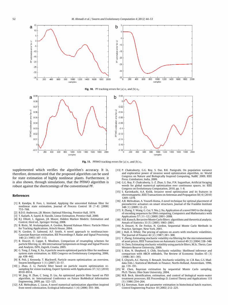
The stochastic differential equations (28a)–(28e) was simulatedusing 2000 steps of the Euler–Maruyamamethod with 1t = 0.1 s.The number of particles was set to 1500 which is relatively lowfor a target tracking problem. The main reason for this choice isto demonstrate the ability of the PFIWO method to estimate thestates of the ballistic object with less number of particles where PFcannot reach an acceptable result. The degeneracy threshold Nthwas selected as 1200, and a systematic re-sampling scheme [7]has been chosen for the PF method. The parameters of the PFIWOalgorithm are given in Table 8. Note that the Max. Weed Numbershould be equal to the number of particles, as it is the case in allof the preceding examples. The target tracking results obtainedusing the PF and PFIWO methodologies are depicted in Fig. 9.The corresponding tracking errors are also provided in Figs. 10and 11. As it is observed from the figures, when the PFIWOscheme is used, the tracking errors are in the satisfactory rangeand PFIWO is capable of tracking the object’s trajectory. On theother hand, large state estimation errors result as the traditional PFalgorithm is utilized. It is obvious that the deteriorated estimationaccuracy of PF is a consequence of the number of particles, whereasthe proposed PFIWO method has preserved its approximationperformance with the same number of particles. Moreover, thenumber of particles has been increased to 3000 and the same

M. Ahmadi et al. / Swarm and Evolutionary Computation 4 (2012) 44–53 51

Fig. 8. The corresponding estimation errors for (a) X , (b) R, (c) S, and (d) P .

Table 8Parameters used in the PFIWO method for the re-entry target tracking problem.

itermax σ0 σf Nmax Nmin Max. weed number

15 0.1 0.000001 4 1 1500

Table 9MAPE performance of PF and PFIWO in 10 simulations pertaining to the re-entrytarget tracking problem.

Estimation method Best Worst Meanx1 (%) x2 (%) x1 (%) x2 (%) x1 (%) x2 (%)

PF 5.47 7.36 12.73 10.48 7.53 8.04PFIWO 2.89 2.36 5.15 6.03 3.33 4.62

Table 10RMSE performance of PF and PFIWO in 10 simulations pertaining to the re-entrytarget tracking problem.

Estimation method Best Worst Meanx1 x2 x1 x2 x1 x2

PF 0.8947 0.9257 2.7435 3.1783 1.0074 1.2715PFIWO 0.1745 0.1011 0.9882 0.9917 0.3078 0.4822

simulations have been launched 10 times. The resultant MAPEand RMSE errors are portrayed in Tables 9 and 10. Once moreas expected, the results sketched in these tables corroborate theclaim that PFIWO results in significant less state approximationerror.

Taken together, the obvious finding that emerges from the setof simulations given in this section is that the proposed PFIWO

Fig. 9. Tracking performance of PF and PFIWO.

method can be applied as a powerful state estimation algorithmin case of model nonlinearity and in the presence of non-Gaussiannoises.

6. Conclusions

An enhanced PF algorithm established upon the IWO schemeis proposed. Firstly, the sampling step is transformed to anoptimization problem by defining an apt fitness function. Then, theIWO algorithm is exploited to deal with the optimization problemefficiently. The results based on the proposed methodology are

52 M. Ahmadi et al. / Swarm and Evolutionary Computation 4 (2012) 44–53

Fig. 10. PF tracking errors for (a) x1 and (b) x2 .

Fig. 11. PFIWO tracking errors for (a) x1 and (b) x2 .

supplemented which verifies the algorithm’s accuracy. It is,therefore, demonstrated that the proposed algorithm can be usedfor state estimation of highly nonlinear plants. Furthermore, itis also shown, through simulations, that the PFIWO algorithm isrobust against the shortcomings of the conventional PF.

References

[1] R. Kandpu, B. Foss, L. Imsland, Applying the unscented Kalman filter fornonlinear state estimation, Journal of Process Control 18 (7–8) (2008)753–768.

[2] B.D.O. Anderson, J.B. Moore, Optimal Filtering, Prentice Hall, 1979.[3] T. Kailath, A. Sayed, B. Hassibi, Linear Estimation, Prentice Hall, 2000.[4] R.J. Elliott, L. Aggoun, J.B. Moore, Hidden Markov Models: Estimation and

Control, third ed., Springer-Verlag, 2008.[5] B. Ristic, M. Arulampalam, A. Gordon, Beyond Kalman Filters: Particle Filters

for Tracking Applications, Artech House, 2004.[6] N. Gordon, D. Salmond, A.F. Smith, A novel approach to nonlinear/non-

Gaussian Bayesian estimation, IEE Proceedings F, Radar and Signal Processing140 (2) (1993) 107–113.

[7] R. Doucet, O. Cappe, E. Moulines, Comparison of resampling schemes forparticle filtering, in: 4th international Symposiumon Image and Signal Processand Analysis, ISPA, Zagreb, Croatia, 2005.

[8] G. Tong, Z. Fang, X. Xu, A particle swarm optimized particle filter for nonlinearsystem state estimation, in: IEEE Congress on Evolutionary Computing, 2006,pp. 438–442.

[9] R. Poli, J. Kennedy, T. Blackwell, Particle swarm optimization: an overview,Swarm Intelligence 1 (1) (2007) 33–57.

[10] J. Zhao, Z. Li, Particle filter based on particle swarm optimization re-sampling for vision tracking, Expert Systems with Applications 37 (12) (2010)8910–8914.

[11] W. Jing, H. Zhao, C. Song, D. Liu, An optimized particle filter based on PSOalgorithm, in: International Conference on Future BioMedical InformationEngineering, 2009, pp. 122–125.

[12] A.R. Mehrabian, C. Lucas, A novel numerical optimization algorithm inspiredfrom weed colonization, Ecological Informatics 1 (4) (2006) 355–366.

[13] P. Chakraborty, G.G. Roy, S. Das, B.K. Panigrahi, On population varianceand explorative power of invasive weed optimization algorithm, in: WorldCongress on Nature and Biologically Inspired Computing, NaBIC 2009, IEEEPress, Coimbatore, India, 2009.

[14] G.G. Roy, P. Chakraborty, S.-Z. Zhao, S. Das, P.N. Suganthan, Artificial foragingweeds for global numerical optimization over continuous spaces, in: IEEECongress on Evolutionary Computation, 2010, pp. 1–8.

[15] S. Karimkashi, A.A. Kishk, Invasive weed optimization and its features inelectromagnetic, IEEE Transactions onAntennas and Propagation 58 (4) (2010)1269–1278.

[16] A.R. Mehrabian, A. Yousefi-Koma, A novel technique for optimal placement ofpiezoelectric actuators on smart structures, Journal of the Franklin Institute348 (1) (2009) 12–23.

[17] X. Zhang, Y.Wang, G. Cui, Y. Niu, J. Xu, Application of a novel IWO to the designof encoding sequences for DNA computing, Computers and Mathematics withApplications 57 (11–12) (2009) 2001–2008.

[18] H.R. Kunsch, RecursiveMonte Carlo filters: algorithms and theoretical analysis,Annals of Statistics 33 (5) (2005) 1983–2001.

[19] A. Doucet, N. De Freitas, N. Gordon, Sequential Monte Carlo Methods inPractice, Springer, New York, 2001.

[20] J. Hull, A. White, The pricing of options on assets with stochastic volatilities,The Journal of Finance 42 (2) (1987) 281–300.

[21] Y. Zheng, Estimating stochastic volatility via filtering for themicromovementsof asset prices, IEEE Transactions on Automatic Control 49 (3) (2004) 338–348.

[22] H. Chen, Estimating stochastic volatility using particle filters,M.Sc. Thesis, CaseWestern Reserve University, 2009.

[23] S. Kim, N. Shepherd, S. Chib, Stochastic volatility: likelihood inference andcomparison with ARCH mModels, The Review of Economic Studies 65 (3)(1998) 361–393.

[24] E. Ghysels, A.C. Harvey, E. Renault, Stochastic volatility, in: C.R. Rao, G.S. Mad-dala (Eds.), Statistical Methods in Finance, North-Holland, Amsterdam, 1996,pp. 119–191.

[25] W. Chen, Bayesian estimation by sequential Monte Carlo sampling,Ph.D. Thesis, Ohio State University, 2004.

[26] M.B. Beck, Identification, estimation, and control of biological waste-watertreatment processes, IEE Proceedings D, Control Theory and Applications 133(5) (1986) 254–264.

[27] K.J. Keesman, State and parameter estimation in biotechnical batch reactors,Control Engineering Practice 10 (2002) 212–225.

M. Ahmadi et al. / Swarm and Evolutionary Computation 4 (2012) 44–53 53

[28] K.V. Gernaey, M.C.M. van Loosdrecht, M. Henze, M. Lind, S.B. Jorgensen,Activated sludge waste-water treatment plant modeling and simula-tion: state of the art, Environmental Modelling and Software 19 (2004)763–783.

[29] K.J. Keesman, H. Spanjers, G. van Straten, Analysis of endogenous processbehavior in activated sludge, Biotechnology and Bioengineering 57 (2) (2000)155–163.

[30] P.J. Costa, Adaptive model architecture and extended Kalman–Bucy filters,IEEE Transactions on Aerospace and Electronic Systems 30 (1994) 525–533.

[31] S.J. Julier, J.K. Uhlmann, Corrections to unscented filtering and nonlinearestimation, Proceedings of the IEEE 92 (2004) 1958–1958.

[32] S. Sarkka, On unscented Kalman filtering for state estimation of continuous-time nonlinear systems, IEEE Transactions on Automatic Control 52 (9) (2007)1631–1640.