SVM and Decision Tree

Machine Learning I CSE 6740, Fall 2013

Le Song

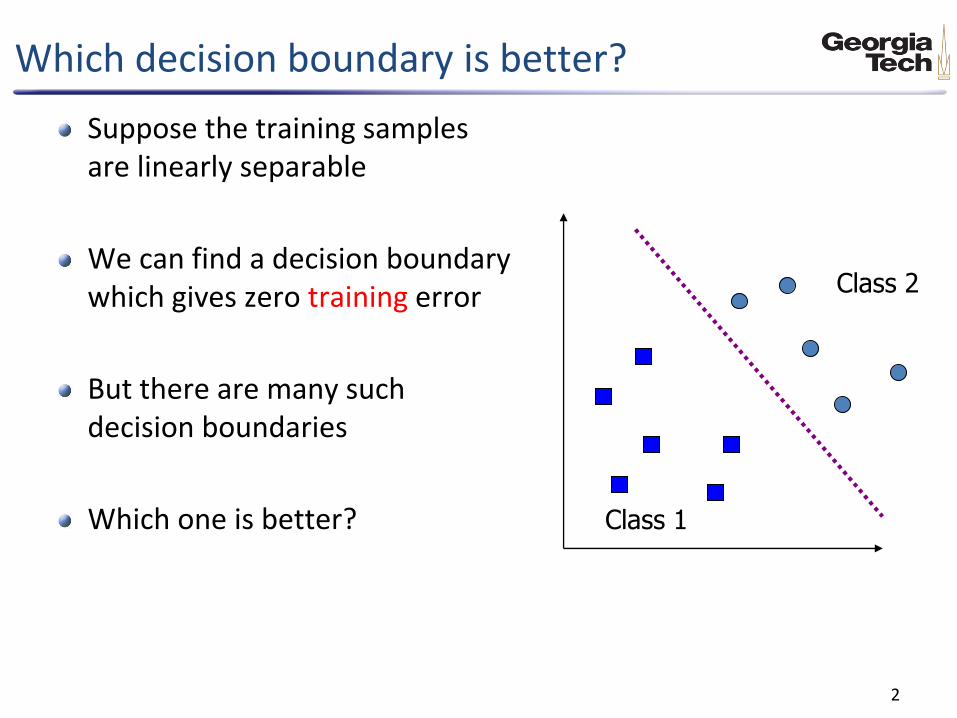
Which decision boundary is better?

Suppose the training samples are linearly separable

We can find a decision boundary which gives zero training error

But there are many such decision boundaries

Which one is better?

2

Class 1

Class 2

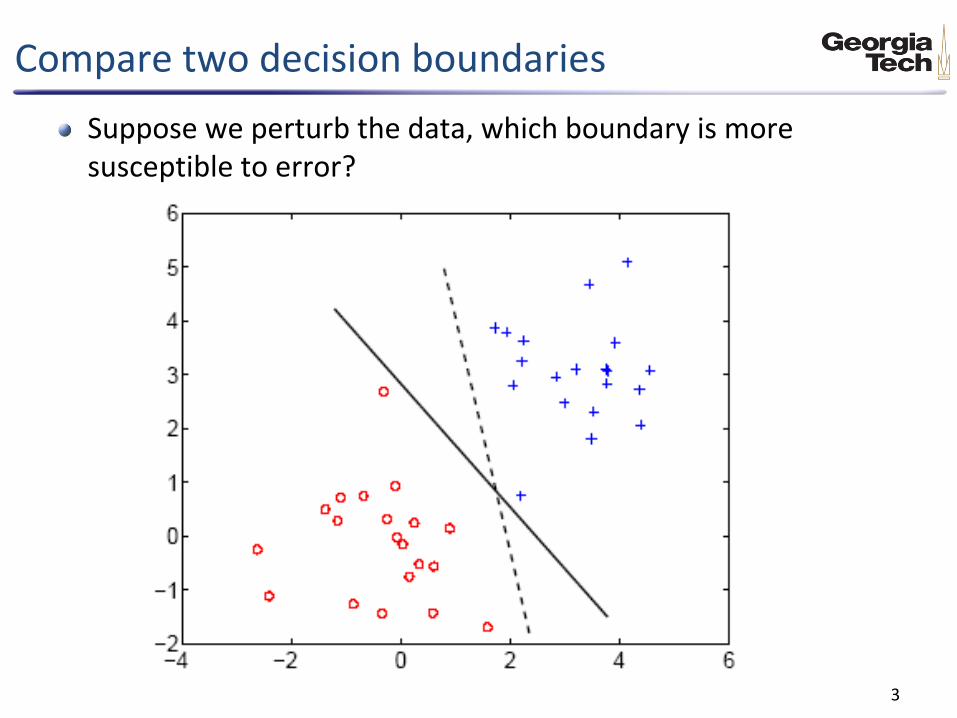
Compare two decision boundaries

Suppose we perturb the data, which boundary is more susceptible to error?

3

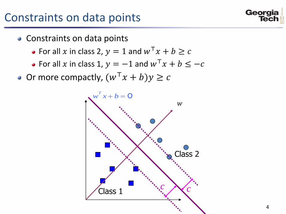
Constraints on data points

Constraints on data points

For all 𝑥 in class 2, 𝑦 = 1 and 𝑤⊤𝑥 + 𝑏 ≥ 𝑐

For all 𝑥 in class 1, 𝑦 = −1 and 𝑤⊤𝑥 + 𝑏 ≤ −𝑐

Or more compactly, (𝑤⊤𝑥 + 𝑏)𝑦 ≥ 𝑐

4

Class 1

Class 2

0 bxwT

c c

𝑤

Classifier margin

Pick two data points 𝑥1 and 𝑥2 which are on each dashed line respectively

The margin is 𝛾 =1

𝑤𝑤⊤ 𝑥1 − 𝑥2 =

2𝑐

| 𝑤 |

5

Class 1

Class 2

0 bxwT

c c

𝑤

𝑥1

𝑥2

Maximum margin classifier

Find decision boundary 𝑤 as far from data point as possible

max𝑤,𝑏 2𝑐

| 𝑤 |

𝑠. 𝑡. 𝑦𝑖 𝑤⊤ 𝑥𝑖 + 𝑏 ≥ 𝑐, ∀𝑖

6

Class 1

Class 2

0 bxwT

c c

𝑤

𝑥1

𝑥2

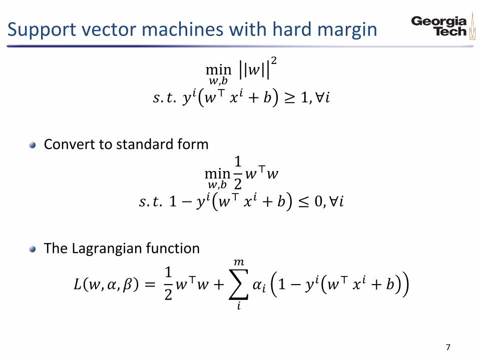
Support vector machines with hard margin

min𝑤,𝑏 𝑤

2

𝑠. 𝑡. 𝑦𝑖 𝑤⊤ 𝑥𝑖 + 𝑏 ≥ 1, ∀𝑖

Convert to standard form

min𝑤,𝑏

1

2𝑤⊤𝑤

𝑠. 𝑡. 1 − 𝑦𝑖 𝑤⊤ 𝑥𝑖 + 𝑏 ≤ 0, ∀𝑖

The Lagrangian function

𝐿 𝑤, 𝛼, 𝛽 = 1

2𝑤⊤𝑤 + 𝛼𝑖 1 − 𝑦

𝑖 𝑤⊤ 𝑥𝑖 + 𝑏

𝑚

𝑖

7

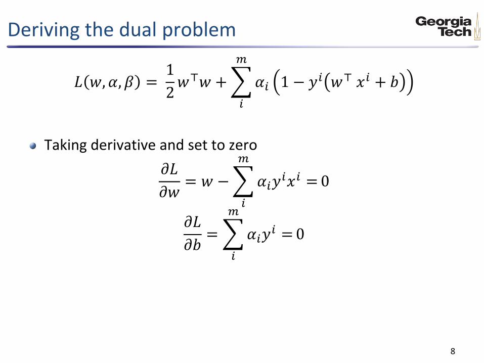
Deriving the dual problem

𝐿 𝑤, 𝛼, 𝛽 = 1

2𝑤⊤𝑤 + 𝛼𝑖 1 − 𝑦

𝑖 𝑤⊤ 𝑥𝑖 + 𝑏

𝑚

𝑖

Taking derivative and set to zero

𝜕𝐿

𝜕𝑤= 𝑤 − 𝛼𝑖𝑦

𝑖𝑥𝑖 =

𝑚

𝑖

0

𝜕𝐿

𝜕𝑏= 𝛼𝑖𝑦

𝑖 =

𝑚

𝑖

0

8

Plug back relation of w and b

𝐿 𝑤, 𝛼, 𝛽 =

1

2 𝛼𝑖𝑦

𝑖𝑥𝑖𝑚𝑖

⊤ 𝛼𝑗𝑦

𝑗𝑥𝑗𝑚𝑗 +

𝛼𝑖 1 − 𝑦𝑖 𝛼𝑗𝑦

𝑗𝑥𝑗𝑚𝑗

⊤ 𝑥𝑖 + 𝑏𝑚

𝑖

After simplification

𝐿 𝑤, 𝛼, 𝛽 = 𝛼𝑖 −

𝑚

𝑖

1

2 𝛼𝑖𝛼𝑗𝑦

𝑖𝑦𝑗 𝑥𝑖⊤𝑥𝑗

𝑚

𝑖,𝑗

9

The dual problem

max𝛼 𝛼𝑖 −

𝑚

𝑖

1

2 𝛼𝑖𝛼𝑗𝑦

𝑖𝑦𝑗 𝑥𝑖⊤𝑥𝑗

𝑚

𝑖,𝑗

𝑠. 𝑡. 𝛼𝑖 ≥ 0, 𝑖 = 1,… ,𝑚

𝛼𝑖𝑦𝑖 =

𝑚

𝑖

0

This is a constrained quadratic programming

Nice and convex, and global maximum can be found

𝑤 can be found as 𝑤 = 𝛼𝑖𝑦𝑖𝑥𝑖𝑚

𝑖

How about 𝑏?

10

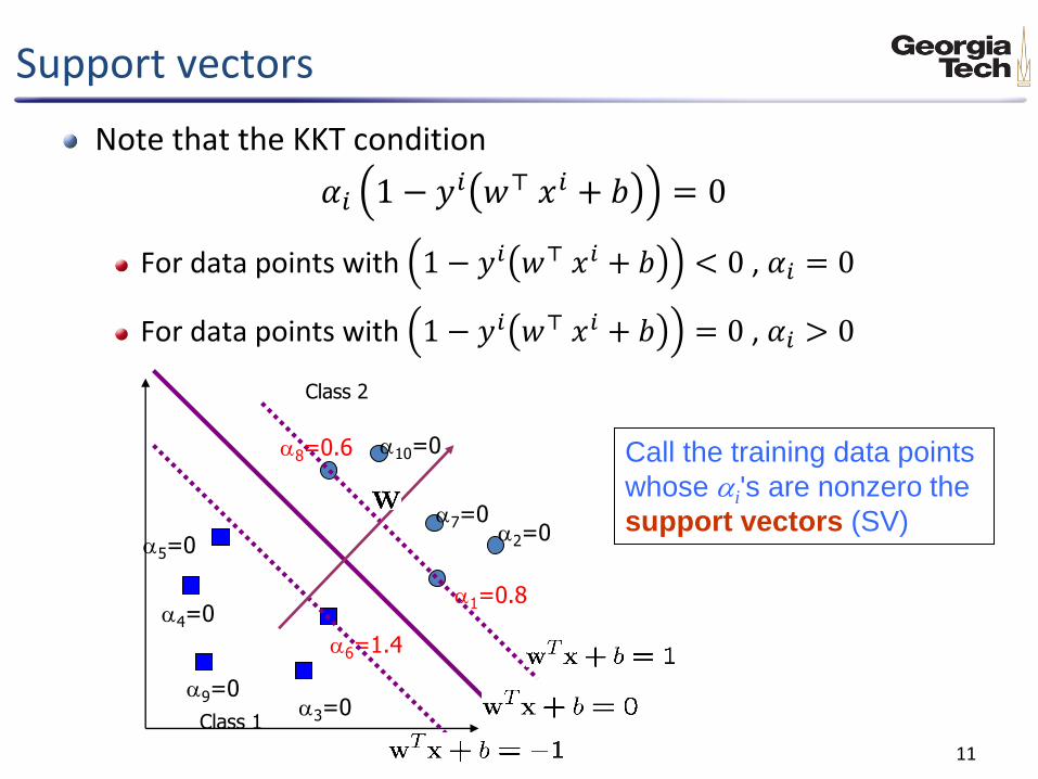
Support vectors

Note that the KKT condition

𝛼𝑖 1 − 𝑦𝑖 𝑤⊤ 𝑥𝑖 + 𝑏 = 0

For data points with 1 − 𝑦𝑖 𝑤⊤ 𝑥𝑖 + 𝑏 < 0 , 𝛼𝑖 = 0

For data points with 1 − 𝑦𝑖 𝑤⊤ 𝑥𝑖 + 𝑏 = 0 , 𝛼𝑖 > 0

11

a6=1.4

Class 1

Class 2

a1=0.8

a2=0

a3=0

a4=0

a5=0

a7=0

a8=0.6

a9=0

a10=0 Call the training data points

whose ai's are nonzero the

support vectors (SV)

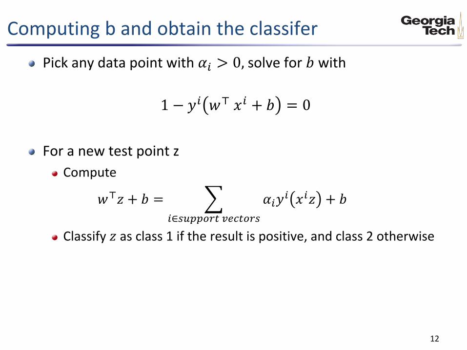
Computing b and obtain the classifer

Pick any data point with 𝛼𝑖 > 0, solve for 𝑏 with

1 − 𝑦𝑖 𝑤⊤ 𝑥𝑖 + 𝑏 = 0

For a new test point z

Compute

𝑤⊤𝑧 + 𝑏 = 𝛼𝑖𝑦𝑖 𝑥𝑖𝑧 + 𝑏

𝑖∈𝑠𝑢𝑝𝑝𝑜𝑟𝑡 𝑣𝑒𝑐𝑡𝑜𝑟𝑠

Classify 𝑧 as class 1 if the result is positive, and class 2 otherwise

12

Interpretation of support vector machines

The optimal w is a linear combination of a small number of data points. This “sparse” representation can be viewed as data compression

To compute the weights 𝛼𝑖, and to use support vector machines we need to specify only the inner products (or

kernel) between the examples 𝑥𝑖⊤𝑥𝑗

We make decisions by comparing each new example z with only the support vectors:

𝑦∗ = 𝑠𝑖𝑔𝑛 𝛼𝑖𝑦𝑖 𝑥𝑖𝑧 + 𝑏

𝑖∈𝑠𝑢𝑝𝑝𝑜𝑟𝑡 𝑣𝑒𝑐𝑡𝑜𝑟𝑠

13

Soft margin constraints

What if the data is not linearly separable?

We will allow points to violate the hard margin constraint (𝑤⊤𝑥 + 𝑏)𝑦 ≥ 1 − 𝜉

14

Class 1

Class 2

0 bxwT

1 1

𝑤

𝜉1

𝜉2 𝜉3

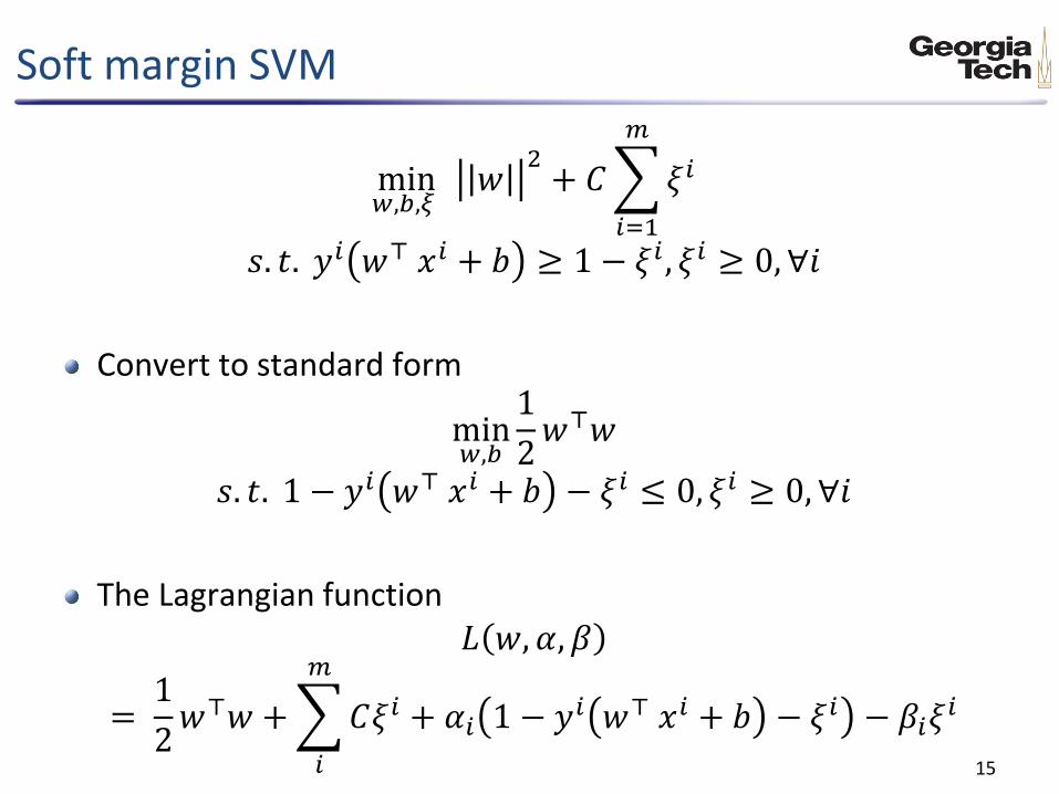
Soft margin SVM

min𝑤,𝑏,𝜉 𝑤

2+ 𝐶 𝜉𝑖

𝑚

𝑖=1

𝑠. 𝑡. 𝑦𝑖 𝑤⊤ 𝑥𝑖 + 𝑏 ≥ 1 − 𝜉𝑖 , 𝜉𝑖 ≥ 0, ∀𝑖

Convert to standard form

min𝑤,𝑏

1

2𝑤⊤𝑤

𝑠. 𝑡. 1 − 𝑦𝑖 𝑤⊤ 𝑥𝑖 + 𝑏 − 𝜉𝑖 ≤ 0, 𝜉𝑖 ≥ 0, ∀𝑖

The Lagrangian function 𝐿 𝑤, 𝛼, 𝛽

= 1

2𝑤⊤𝑤 + 𝐶𝜉𝑖 + 𝛼𝑖 1 − 𝑦

𝑖 𝑤⊤ 𝑥𝑖 + 𝑏 − 𝜉𝑖𝑚

𝑖

− 𝛽𝑖𝜉𝑖

15

Deriving the dual problem

𝐿 𝑤, 𝛼, 𝛽

= 1

2𝑤⊤𝑤 + 𝐶𝜉𝑖 + 𝛼𝑖 1 − 𝑦

𝑖 𝑤⊤ 𝑥𝑖 + 𝑏 − 𝜉𝑖𝑚

𝑖

− 𝛽𝑖𝜉𝑖

Taking derivative and set to zero

𝜕𝐿

𝜕𝑤= 𝑤 − 𝛼𝑖𝑦

𝑖𝑥𝑖 =

𝑚

𝑖

0

𝜕𝐿

𝜕𝑏= 𝛼𝑖𝑦

𝑖 =

𝑚

𝑖

0

𝜕𝐿

𝜕𝜉𝑖 = 𝐶 − 𝛼𝑖 − 𝛽𝑖 = 0

16

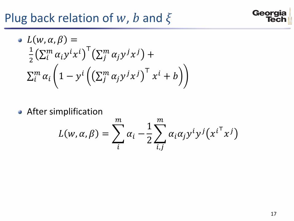
Plug back relation of 𝑤, 𝑏 and 𝜉

𝐿 𝑤, 𝛼, 𝛽 =

1

2 𝛼𝑖𝑦

𝑖𝑥𝑖𝑚𝑖

⊤ 𝛼𝑗𝑦

𝑗𝑥𝑗𝑚𝑗 +

𝛼𝑖 1 − 𝑦𝑖 𝛼𝑗𝑦

𝑗𝑥𝑗𝑚𝑗

⊤ 𝑥𝑖 + 𝑏𝑚

𝑖

After simplification

𝐿 𝑤, 𝛼, 𝛽 = 𝛼𝑖 −

𝑚

𝑖

1

2 𝛼𝑖𝛼𝑗𝑦

𝑖𝑦𝑗 𝑥𝑖⊤𝑥𝑗

𝑚

𝑖,𝑗

17

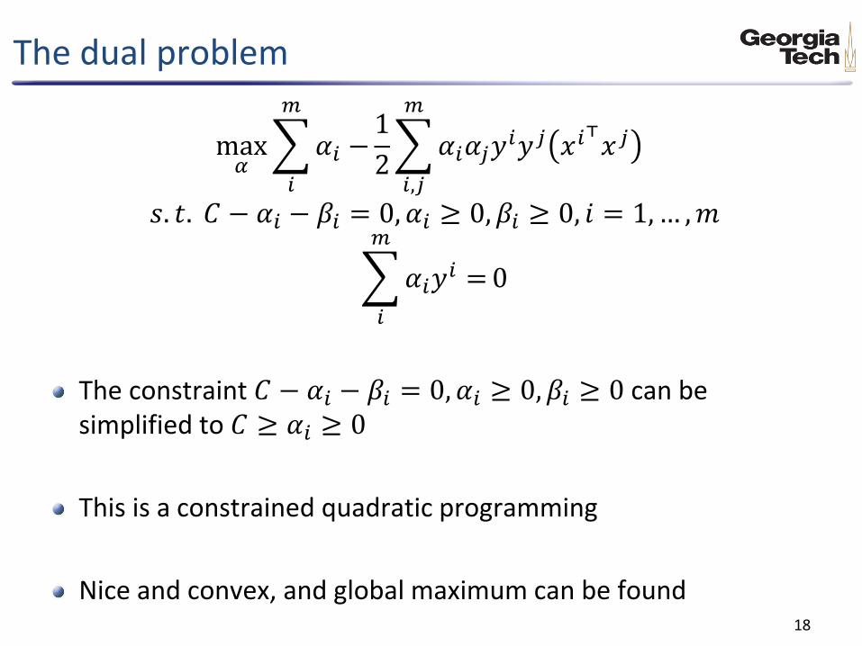
The dual problem

max𝛼 𝛼𝑖 −

𝑚

𝑖

1

2 𝛼𝑖𝛼𝑗𝑦

𝑖𝑦𝑗 𝑥𝑖⊤𝑥𝑗

𝑚

𝑖,𝑗

𝑠. 𝑡. 𝐶 − 𝛼𝑖 − 𝛽𝑖 = 0, 𝛼𝑖 ≥ 0, 𝛽𝑖 ≥ 0, 𝑖 = 1,… ,𝑚

𝛼𝑖𝑦𝑖 =

𝑚

𝑖

0

The constraint 𝐶 − 𝛼𝑖 − 𝛽𝑖 = 0, 𝛼𝑖 ≥ 0, 𝛽𝑖 ≥ 0 can be simplified to 𝐶 ≥ 𝛼𝑖 ≥ 0

This is a constrained quadratic programming

Nice and convex, and global maximum can be found

18

Learning nonlinear decision boundary

Linearly separable

Nonlinearly separable

19

The XOR gate Speech recognition

A decision tree for Tax Fraud

Input: a vector of attributes 𝑋 = [Refund,MarSt,TaxInc]

Output: 𝑌= Cheating or Not

H as a procedure:

20

Refund

MarSt

TaxInc

YES NO

NO

NO

Yes No

Married Single, Divorced

< 80K > 80K

Each internal node: test one attribute 𝑋𝑖 Each branch from a node: selects one value for 𝑋𝑖 Each leaf node: predict 𝑌

Apply model to test data I

21

Refund

MarSt

TaxInc

YES NO

NO

NO

Yes No

Married Single, Divorced

< 80K > 80K

R e fu n d M a r ita l

S ta tu s

T a x a b le

In c o m e C h e a t

N o M a rr ie d 8 0 K ? 10

Query Data

Start from the root of tree.

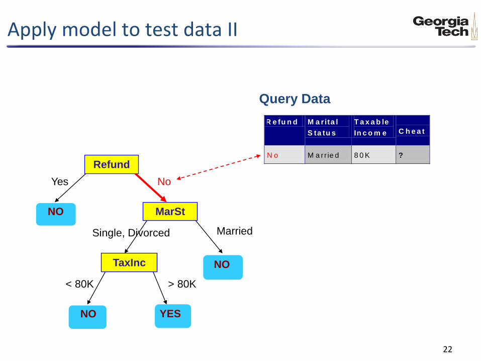
Apply model to test data II

22

Refund

MarSt

TaxInc

YES NO

NO

NO

Yes No

Married Single, Divorced

< 80K > 80K

R e fu n d M a r ita l

S ta tu s

T a x a b le

In c o m e C h e a t

N o M a rr ie d 8 0 K ? 10

Query Data

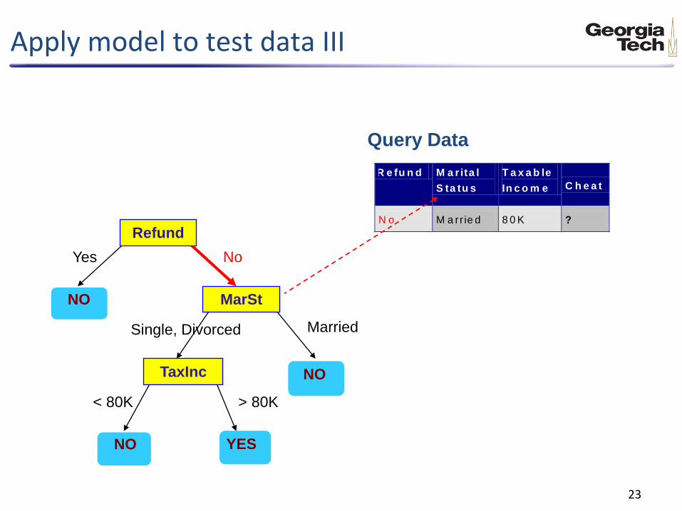
Apply model to test data III

23

Refund

MarSt

TaxInc

YES NO

NO

NO

Yes No

Married Single, Divorced

< 80K > 80K

R e fu n d M a r ita l

S ta tu s

T a x a b le

In c o m e C h e a t

N o M a rr ie d 8 0 K ? 10

Query Data

Apply model to test data IV

24

Refund

MarSt

TaxInc

YES NO

NO

NO

Yes No

Married Single, Divorced

< 80K > 80K

R e fu n d M a r ita l

S ta tu s

T a x a b le

In c o m e C h e a t

N o M a rr ie d 8 0 K ? 10

Query Data

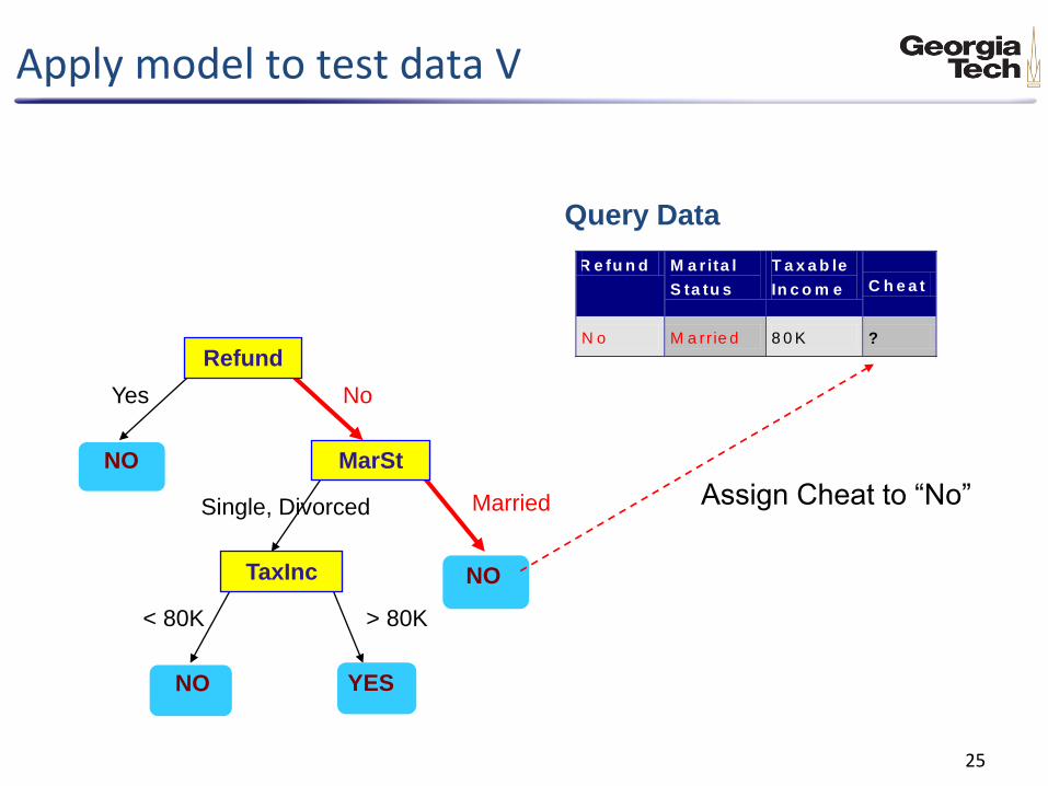
Apply model to test data V

25

Refund

MarSt

TaxInc

YES NO

NO

NO

Yes No

Married Single, Divorced

< 80K > 80K

R e fu n d M a r ita l

S ta tu s

T a x a b le

In c o m e C h e a t

N o M a rr ie d 8 0 K ? 10

Query Data

Assign Cheat to “No”

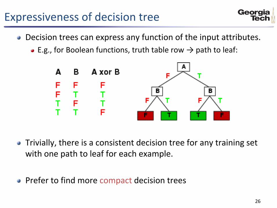
Expressiveness of decision tree

Decision trees can express any function of the input attributes.

E.g., for Boolean functions, truth table row → path to leaf:

Trivially, there is a consistent decision tree for any training set with one path to leaf for each example.

Prefer to find more compact decision trees

26

Hypothesis spaces (model space

How many distinct decision trees with n Boolean attributes?

= number of Boolean functions

= number of distinct truth tables with 2n rows = 22n

E.g., with 6 Boolean attributes, there are 18,446,744,073,709,551,616 trees

How many purely conjunctive hypotheses (e.g., Hungry Rain)?

Each attribute can be in (positive), in (negative), or out 3n distinct conjunctive hypotheses

More expressive hypothesis space increases chance that target function can be expressed

increases number of hypotheses consistent with training set

may get worse predictions

27

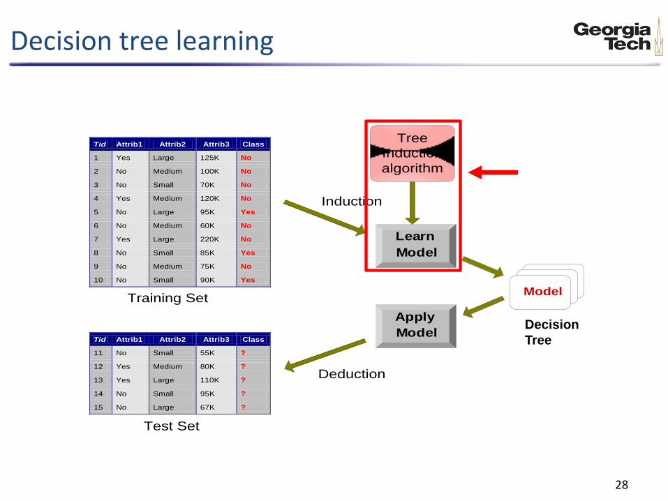
Decision tree learning

28

Apply

Model

Induction

Deduction

Learn

Model

Model

Tid Attrib1 Attrib2 Attrib3 Class

1 Yes Large 125K No

2 No Medium 100K No

3 No Small 70K No

4 Yes Medium 120K No

5 No Large 95K Yes

6 No Medium 60K No

7 Yes Large 220K No

8 No Small 85K Yes

9 No Medium 75K No

10 No Small 90K Yes 10

Tid Attrib1 Attrib2 Attrib3 Class

11 No Small 55K ?

12 Yes Medium 80K ?

13 Yes Large 110K ?

14 No Small 95K ?

15 No Large 67K ? 10

Test Set

Tree

Induction

algorithm

Training Set

Decision

Tree

Example of a decision tree

29

T id R e fu n d M a rita l

S ta tu s

T a x a b le

In c o m e C h e a t

1 Y e s S in g le 1 2 5 K N o

2 N o M a rr ie d 1 0 0 K N o

3 N o S in g le 7 0 K N o

4 Y e s M a rr ie d 1 2 0 K N o

5 N o D iv o rc e d 9 5 K Y e s

6 N o M a rr ie d 6 0 K N o

7 Y e s D iv o rc e d 2 2 0 K N o

8 N o S in g le 8 5 K Y e s

9 N o M a rr ie d 7 5 K N o

1 0 N o S in g le 9 0 K Y e s10

Refund

MarSt

TaxInc

YES NO

NO

NO

Yes No

Married Single, Divorced

< 80K > 80K

Splitting Attributes

Training Data Model: Decision Tree

Another example of a decision tree

30

MarSt

Refund

TaxInc

YES NO

NO

NO

Yes No

Married Single,

Divorced

< 80K > 80K

There could be more than one tree that

fits the same data!

T id R e fu n d M a rita l

S ta tu s

T a x a b le

In c o m e C h e a t

1 Y e s S in g le 1 2 5 K N o

2 N o M a rr ie d 1 0 0 K N o

3 N o S in g le 7 0 K N o

4 Y e s M a rr ie d 1 2 0 K N o

5 N o D iv o rc e d 9 5 K Y e s

6 N o M a rr ie d 6 0 K N o

7 Y e s D iv o rc e d 2 2 0 K N o

8 N o S in g le 8 5 K Y e s

9 N o M a rr ie d 7 5 K N o

1 0 N o S in g le 9 0 K Y e s10

Training Data

Top-Down Induction of Decision tree

Main loop:

𝐴 ← the “best” decision attribute for next node

Assign A as the decision attribute for node

For each value of A, create new descendant of node

Sort training examples to leaf nodes

If training examples perfectly classified, then STOP;

ELSE iterate over new leaf nodes

31

Tree Induction

Greedy strategy.

Split the records based on an attribute test that optimizes certain criterion.

Issues

Determine how to split the records

How to specify the attribute test condition?

How to determine the best split?

Determine when to stop splitting

32

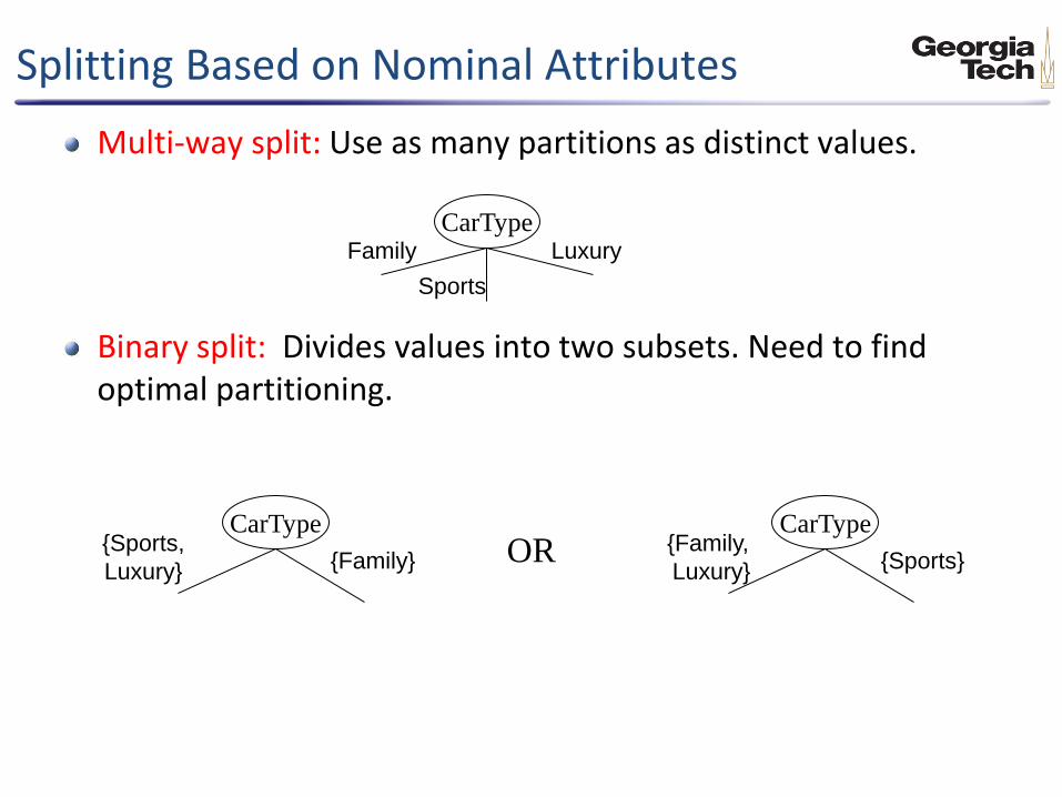
Multi-way split: Use as many partitions as distinct values.

Binary split: Divides values into two subsets. Need to find optimal partitioning.

CarType Family

Sports

Luxury

CarType {Family,

Luxury} {Sports}

CarType {Sports,

Luxury} {Family} OR

Splitting Based on Nominal Attributes

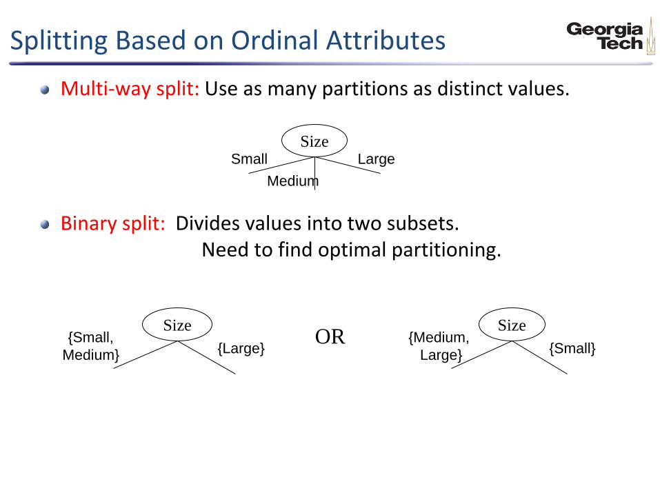
Multi-way split: Use as many partitions as distinct values.

Binary split: Divides values into two subsets. Need to find optimal partitioning.

Size Small

Medium

Large

Size {Medium,

Large} {Small}

Size {Small,

Medium} {Large} OR

Splitting Based on Ordinal Attributes

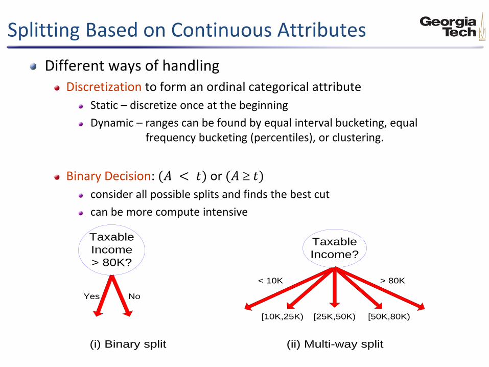
Different ways of handling Discretization to form an ordinal categorical attribute

Static – discretize once at the beginning

Dynamic – ranges can be found by equal interval bucketing, equal frequency bucketing (percentiles), or clustering.

Binary Decision: (𝐴 < 𝑡) or (𝐴 𝑡)

consider all possible splits and finds the best cut

can be more compute intensive

Splitting Based on Continuous Attributes

Taxable

Income

> 80K?

Yes No

Taxable

Income?

(i) Binary split (ii) Multi-way split

< 10K

[10K,25K) [25K,50K) [50K,80K)

> 80K

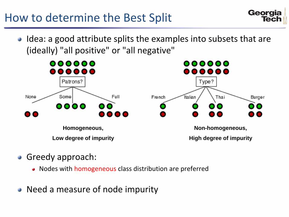
How to determine the Best Split

Idea: a good attribute splits the examples into subsets that are (ideally) "all positive" or "all negative"

Greedy approach: Nodes with homogeneous class distribution are preferred

Need a measure of node impurity

Non-homogeneous,

High degree of impurity

Homogeneous,

Low degree of impurity

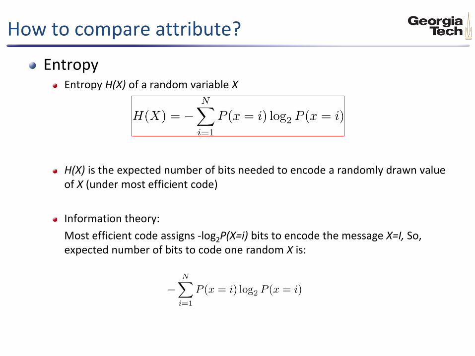
How to compare attribute?

Entropy Entropy H(X) of a random variable X

H(X) is the expected number of bits needed to encode a randomly drawn value of X (under most efficient code)

Information theory:

Most efficient code assigns -log2P(X=i) bits to encode the message X=I, So, expected number of bits to code one random X is:

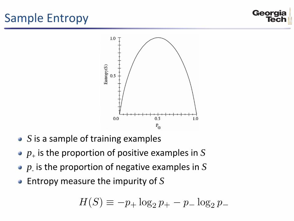
Sample Entropy

S is a sample of training examples

p+ is the proportion of positive examples in S

p- is the proportion of negative examples in S

Entropy measure the impurity of S

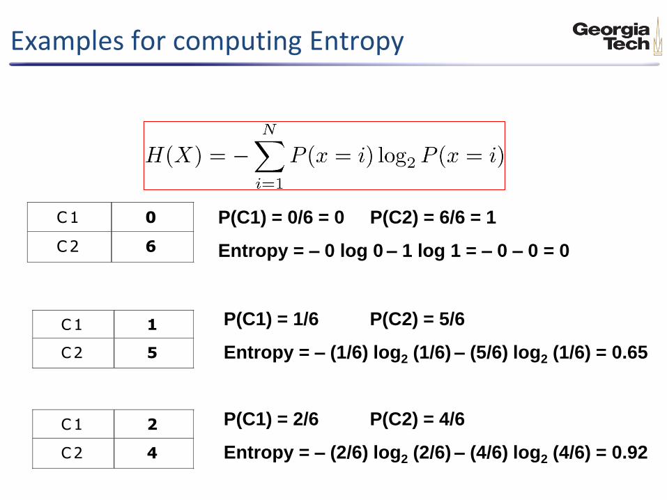
Examples for computing Entropy

C 1 0

C 2 6

C 1 2

C 2 4

C 1 1

C 2 5

P(C1) = 0/6 = 0 P(C2) = 6/6 = 1

Entropy = – 0 log 0 – 1 log 1 = – 0 – 0 = 0

P(C1) = 1/6 P(C2) = 5/6

Entropy = – (1/6) log2 (1/6) – (5/6) log2 (1/6) = 0.65

P(C1) = 2/6 P(C2) = 4/6

Entropy = – (2/6) log2 (2/6) – (4/6) log2 (4/6) = 0.92

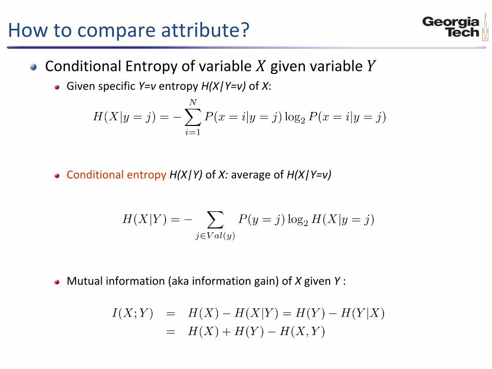
How to compare attribute?

Conditional Entropy of variable 𝑋 given variable 𝑌 Given specific Y=v entropy H(X|Y=v) of X:

Conditional entropy H(X|Y) of X: average of H(X|Y=v)

Mutual information (aka information gain) of X given Y :

Information Gain

Information gain (after split a node):

𝑛 samples in parent node 𝑝 is split into 𝑘 partitions; 𝑛𝑖 is number of records in partition 𝑖

Measures Reduction in Entropy achieved because of the split. Choose the split that achieves most reduction (maximizes GAIN)

k

i

i

splitiEntropy

n

npEntropyGAIN

1

)()(

Problem of splitting using information gain

Disadvantage: Tends to prefer splits that result in large number of partitions, each being small but pure.

Gain Ratio:

Adjusts Information Gain by the entropy of the partitioning (SplitINFO). Higher entropy partitioning (large number of small partitions) is penalized!

Used in C4.5

Designed to overcome the disadvantage of Information Gain

42

SplitINFO

GAINGainRATIO

Split

split

k

i

ii

n

n

n

nSplitINFO

1

log

Stopping Criteria for Tree Induction

Stop expanding a node when all the records belong to the same class

Stop expanding a node when all the records have similar attribute values

Early termination (to be discussed later)

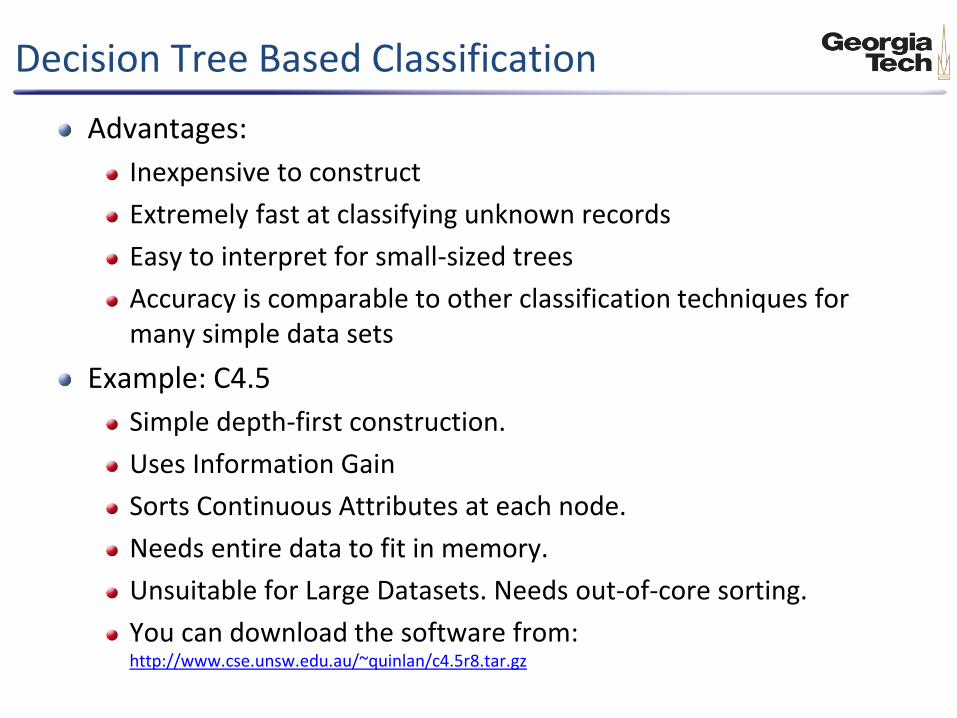
Decision Tree Based Classification

Advantages:

Inexpensive to construct

Extremely fast at classifying unknown records

Easy to interpret for small-sized trees

Accuracy is comparable to other classification techniques for many simple data sets

Example: C4.5

Simple depth-first construction.

Uses Information Gain

Sorts Continuous Attributes at each node.

Needs entire data to fit in memory.

Unsuitable for Large Datasets. Needs out-of-core sorting.

You can download the software from: http://www.cse.unsw.edu.au/~quinlan/c4.5r8.tar.gz