Embed Size (px)
Citation preview

Sustainable Engineering Internship
2018 Final Report
July 15th, 2018
Jacob Shactman, Gabby Peralta, Laurel He, Takeru Nishi
1

SEI 2018 Draft Report
Table of Contents List of Figures 5
List Of Tables 7
Executive Summaries 9
Assignment 1: Green Grid Performance/Solar Powered Salt Water Pump 11 1.1 Background 11 1.2 Purpose 12 1.3 Scope 13 1.4 Methods 13 1.5 Results and Analysis 16 1.6 Conclusions and Recommendations 22 1.7 References 23
Assignment 2: Adjusting Depth of Discharge in the ECB Batteries 24 2.1 Background 24 2.2 Purpose 24 2.3 Scope 25 2.4 Methods 25 2.5 Results and Analysis 26 2.6 Conclusions and Recommendations 32 2.7 References 32
Assignment 3: Analysis of SML’s Solar Arrays 33 3.1 Background 33 3.2 Purpose 33 3.3 Scope 33 3.4 Methods 34 3.5 Results and Analysis 40 3.6 Conclusions and Recommendations 53 3.7 References 54
Assignment 4: Refrigeration Upgrade 55 4.1 Background 55 4.2 Purpose 56 4.3 Scope 57 4.4 Methods 57
2

SEI 2018 Draft Report
4.5 Results and Analysis 59 4.6 Conclusions and Recommendations 72 4.7 References 72
Assignment 5: Wastewater - Solids Solutions 74 5.1 Background 74 5.2 Purpose 75 5.3 Scope 75 5.4 Methods 75 5.5 Results and Analysis 76 5.6 Conclusions and Recommendations 81 5.7 References 81
Assignment 6: Rooftop Water for Flushing Toilets in Dorm 1, 2 and 3 82 6.1 Background 82 6.2 Purpose 82 6.3 Scope 82 6.4 Methods 82 6.5 Results and Analysis 84 6.6 Conclusions and Recommendations 88 6.7 References 89
Assignment 7: Appledore Transportation Analysis 90 7.1 Background 90 7.2 Purpose 90 7.3 Scope 90 7.4 Methods 91 7.5 Results and Analysis 92 7.6 Conclusions and Recommendations 97 7.7 References 100
Assignment 8: Well Drawdown Test 101 8.1 Background 101 8.2 Purpose 102 8.3 Scope 103 8.4 Methods 103 8.4.1. Data Acquisition 103 8.4.2. Data Analysis 104 8.5 Results and Analysis 104
3

SEI 2018 Draft Report
8.6 Conclusions and Recommendations 112 8.7 References 113
4

SEI 2018 Draft Report
List of Figures Figure 1: Original MREU Setup Figure 2: Orientation and Numbering of Solar Arrays on the North West Side Figure 3: Orientation and Numbering of Solar Arrays on the South East Side Figure 4: Battery Voltage for when the K-House System was kept on all night Figure 5: Plot of Output for the numbered Charge Controllers for July 4th Figure 6: Plot of Output for the numbered Charge Controllers for June 5th Figure 7: Comparison of the Battery Voltages the day after being utilized all night Figure 8: State of Charge for July 3rd to 9th at a Start SOC of 62% and Stop SOC of 67% Figure 9: Lifespan related to Depth of Discharge Figure 10: Decline in Cost of Lithium Ion Batteries. Graph from a Bloomberg New Energy Finance survey Figure 11: Layout and Numbering of the Northern Solar Arrays Figure 12: Layout of Southern Solar Arrays Figure 13: Tightening Bolts Figure 14: Tilt Angle (left) measured as Dip; Array Position (right) measured as Plunge Figure 15. Example I-V Load Curves for CanadianSolar--CS6X 305P. Figure 16: Graph for each Charge Controller of K-House for June 29th Figure 17: Representation of how a Refrigeration System Works Figure 18: Graph of Energy Consumption of the Fridge Compressor over several Hours Figure 19: Temperatures for Kitchen, Fridge, and Freezer Figure 20: CAD of the Refrigerator and Freezer System Figure 21: IR Picture showing Cold Seeping under the Door Figure 22: Refrigerator Compressors Figure 23: A Layout of the Top Wall Figure 24: A Layout of the Back Wall Figure 25: A Layout of the Side Walls Figure 26: Infrared Picture of Left Outside Wall of System Figure 27: KE2Therm Evaporator Efficiency Device Figure 28: Representation of how the Refrigerator System Operates Figure 30: Schematic of the SludgeHammer System Figure 31: Sludge Depths in Tank 1 Figure 32: Sludge Depths in Tank 2 Figure 33: Single axle trailer being pulled by the tractor Figure 34: Tractor Usage Figure 35: Heavy rusting on the underbody Figure 36: Truck Usage
5

SEI 2018 Draft Report
Figure 37: Gator Usage Figure 38. Map of Appledore Island with important geologic features. Figure 39: Main Production Well Pumping Test Figure 40: Main Production Well Water Level vs. Time (January - July 2018) Figure 41. The Electrical Resistivity Imaging of the Main Well and the 6-foot Test Well Figure 42. 2017 Pumping Test Result: Water Level Changes for Main Well and 6-foot Test Well
6
SEI 2018 Draft Report
List Of Tables Table 1: Array Pairs that correspond to each Charge Controller Table 2: Power at Low and High Tides Table 3: Average Power at Low and High Tides Table 4: Values to Analyze Island Grid Table 5: Percentage of Island Load from the Generator Table 6: Total Power Output for each Charge Controller on July 4th Table 7: Total Power Output for each Charge Controller on June 5th Table 8: Average Battery Cycles per Day for each DOD Table 9: Graph showing relationship between DOD and Lifespan Table 10: Percentage of Island Load Relying on Non-Renewable Energy and Average Generator Run Time Table 11. Costs of Generator Diesel for various Depth of Discharge Table 12: Battery Cost Estimate Assuming the Cost of Lithium Ion Batteries Stay the Same Table 13: Battery Cost Estimate Assuming the Cost of Lithium Ion Batteries Decrease by 2% each Year Table 14: Pyranometer for the Time when the Interns Collected Solar Array Data Table 15. Voc and Isc Manufacturer Specs Data for Solar Arrays Table 16: Current and Voltage of the Southern Arrays Table 17: Current and Voltage for Northern Arrays Table 18: Actual Power Output of Southern Arrays Table 19: Actual Power Output of Northern Arrays Table 20: Actual Efficiencies of Northern Arrays Table 21: Actual Efficiencies of Southern Arrays Table 22: Max Power Per Location Table 23: Efficiencies of Solar Arrays based on Manufacturer Table 24: Temperature of each Array and the Efficiency Lost from Increase Temperature Table 25: Corrected Efficiency from Temperature Increase for Northern Arrays Table 26: Corrected Efficiency from Temperature Increase for Southern Arrays Table 27. Solar Array Orientations and Tilt Angles Table 28. Ideal Solar Array Orientations and Tilt Angles at Latitude 43°N Table 28. Range of Temperature Correction for Northern Solar Arrays Table 29: Range of Temperature Correction for Southern Solar Arrays Table 30. Range of Performance Coefficient for Northern Solar Arrays Table 31. Range of Performance Coefficient for Southern Solar Arrays Table 32. Summary of Average Efficiency, Performance Coefficient and PV Panel Type Table 33: Nameplate Data of Refrigerator and Freezer Table 34: Defining the Model Number for the Refrigerator and Freezer
7

SEI 2018 Draft Report
Table 35: Energy Consumption for Fridge Table 36: Energy Consumption for Freezer Table 37: Temperature Statistics for the Refrigerator, Freezer, and Kitchen Table 38: Outside Dimensions of the System Table 39: Inside Fridge Dimensions Table 40: Freezer Dimensions Table 41: Evaluation of Potential Refrigerant Replacements Table 42: Temperature of the Outside Walls Table 43: Inside Temperature of Fridge and Freezer Walls Table 44: Amount of Solids Before SludgeHammer Installation Table 45: Biological Oxygen Demand Table 46: Total Suspended Solids Table 47: Flush Count (2018) Table 48: Water Usage per Person (2018) Table 49: Gutters around 1 dorm building - 1 cistern/pumping system to supply 3 dorms Table 50: Gutters around 1 Building Supplying Dorms 2 & 3 Table 51: Gutters around half of one dorm - 3 cisterns to supply each dorm respectively Table 52: Inventory Table 53: Tractor Usage Table 54: Trailer Usage Table 55: Truck usage Table 56: Gator Usage Table 57: Utility Vehicle Design Matrix Table 58. Computed Specific Yield Table 59. Daily Drinking Water Usage, June, 2018
8

SEI 2018 Draft Report
Executive Summaries Assignment 1: Green Grid Performance/Solar Powered Salt Water Pump The interns were tasked with analyzing the new solar set up placed on Kingsbury House to power the salt water pump. Last years interns predicted the system to be able to power the pump throughout the night, and that the reliance on non-renewable energy would go from 40% to 17%. The interns spent the night in K-House to see if the system could get through the night, which it successfully did. The reliance is down to 28%, but it is predicted to go much more after the automatic switchover is implemented. The differing solar array orientations were graphed, where the interns found the system outputted power throughout the entire day, with different orientations have its max power output at different times. The noise and heat were also proven to not be a problem. Assignment 2: Adjusting the Depth of Discharge in the ECB Batteries The interns last year counted the number of cycles, and the corresponding lifespan on the batteries at certain depth of discharges. Using the manufacturer specs, the 2017 interns found the seasons left at different depth of discharges. This year the interns actually changed the depth of discharge on the ECB batteries. Using this years and previous years datasets, the interns concluded that 33% was a suitable DOD for the next 10 years. The interns also proposed that these batteries, when it was time to be replaced, should be with Lithium Ion batteries, since they are more resilient, have longer lifespans, and are technologically advancing. The interns also recommend that this project be repeated after the MREU system has been fully integrated.
Assignment 3: Analysis of SML’s Solar Arrays
The interns this year were tasked to assess the efficiency of the solar arrays throughout the island. Actual power output was measured from the solar combiner boxes as voltage and current, and this is compared to theoretical power output from specs. Factors reducing the efficiency of the solar arrays were also taken into account, such as overheating, shading, maintenance, tilt angle and orientation, and time since installation. The interns also offered potential solutions to the reduced efficiency.
9

SEI 2018 Draft Report
Assignment 4: Refrigeration Upgrade
Shoals Marine Lab has had the same refrigeration system since original installation in the mid 1970’s. The entire system, ranging from the insulation to the compressors in the basement, is showing signs of wear and tear. Since no information was gathered on the system components prior to this year, interns were tasked with documenting and assessing all parts of the refrigeration system. Two plans of action were proposed; the first is component replacement and the second is complete reconstruction. Since SML may choose either plan of action, detailed suggestions were made for each.
Assignment 5: Wastewater - Solid Solutions
Wastewater is one of the key components of SML’s infrastructure. Disposal of wastewater has proven to be a significant financial burden, leading island staff to invest in novel treatment methods. A few years ago, SML invested in composting toilets following the recommendation of the sustainable engineering interns; these toilets proved to be a viable alternative to traditional septic system. This technology, however, cannot be implemented everywhere on the island, so treatment of solids in the existing septic tanks is necessary. This year, interns analyzed the progress of the SludgeHammer aerobic digestion contraption. The company’s CEO and New England distributor both claim that this treatment apparatus is able to clean sludge from septic tanks so thoroughly that the need to pump the tanks is eliminated. Biological oxygen demand (BOD) and total suspended solids (TSS) tests, as well as daily sludge measurements were done. With the short amount of time between installation and conclusion of the program, interns were unable to gather enough information to reach a definitive conclusion about the success of the system, so further monitoring and testing is necessary. Assignment 6: Rooftop Water for Flushing Toilets in Dorm 1, 2 and 3 With very limited freshwater resources on Appledore Island, removing demand from the well is essential to decrease the likelihood of having to utilize the energy intensive reverse osmosis system. One way to decrease this demand on the well is to collect rainwater for flushing within the dorms. This has been done successfully in Bartels Hall, however, interns this year looked at designing a system specifically for the dorm buildings.
10

SEI 2018 Draft Report
Assignment 7: Appledore Transportation Analysis Because Appledore Island is remote and isolated from the mainland, transportation to, from, and around the island is imperative for daily island operation. Many challenges exist on Appledore such as the rough terrain and the corrosive marine environment. Interns were tasked with assessing the current transportation means and methods. Along with this, recommendations were made to optimize and improve these systems.
Assignment 8: Well Drawdown Test
As a continuous effort to better understand the main well aquifer, the interns this year conducted a well drawdown test in order to determine hydraulic properties. The results yielded qualitative conclusions about the limited extent of the aquifer and a constant seepage rate. The interns used test results from 2016 and 2017 to compute the aquifer capacity. Insights were also shed on the geological background of Appledore island and the nature of the aquifer.
11

SEI 2018 Draft Report
Assignment 1: Green Grid Performance/Solar Powered Salt Water Pump Project Leads: Gabby Peralta and Takeru Nishi 1.1 Background SML received a donation of a Mobile Renewable Energy Unit (MREU) in 2017 from a Cornell alumnus, Sean O’Day. Although originally planned for military use in arid and remote desert conditions, the unit had to be reconfigured to allow for all components to be installed in the Kingsbury house. The solar panels were placed on the either side of the roof, and the batteries, charge controllers, and inverters were placed in the basement. This new setup allowed for consolidation of the unit into one confined area. A graphic of the original MREU setup is shown in figure 1.
Prior to the interns’ arrival, SML installed the 100 solar panels capable of producing 30 kilowatts, 80 kilowatt-hours of energy storage (16 lithium ion batteries), 10 solar charge controllers, and 7 inverters on/in the K-House in order to power the lab’s saltwater pump. During the week of the interns’ arrival, the K-house grid was powered on for the first time. Within the first day of operation, the system’s programming showed a reluctance to joining the main green
12
SEI 2018 Draft Report
grid. Ideally, the saltwater pump would run off of the K-house grid until the batteries reached a certain depth of discharge, triggering an automated rerouting of the pump load power to the main grid. This process would be instantaneous, and the pump would continue to operate uninterrupted. However, a yet undetermined issue in either the system programming or wiring is preventing this automation. For this reason, island engineers have been manually switching the power from the K-house grid to the green grid, avoiding the possibility of running the batteries too low. This year, the interns wish to analyze data from the newly installed grid with the help of Schneider Electric’s data monitor. Interns hope to see that the new system does improve the island green energy use from 60% to 83%, as suggested by the 2017 interns. Interns also observed the rate at which the batteries are charged on an ideal solar day and determined how long the batteries can power the salt water pump. All of the island solar arrays, except those installed on the Kingsbury house (K-house), have been oriented towards the south east. On K-house, there are 14 arrays for the new system. Arrays 8 through 14 face southeast, arrays 1 through 7 on the other side of the roof face northwest, and arrays 1 through 5 are situated on the porch roof at a much shallower angle. The interns graphed each solar array output to see the discrepancies. The interns placed a data monitor on the saltwater pump to determine the load and to see if the load changed with the tide. Since residents live above the MREU in K-House, it is important to record the noise level coming from the basement. The added activity in the basement also increases the temperature, so the optimal and extreme temperatures for the batteries were calculated. 1.2 Purpose Since the 2017 intern report on the green grid and MREU consisted entirely of literature values, one of the main deliverables of this year’s assignment is to compare and contrast the data collected during these past few weeks with that of last year. This comparison may help to answer the question of if this new system will provide enough energy to keep the generator off at night.
13

SEI 2018 Draft Report
1.3 Scope Of the many values calculated by the 2017 interns, the most intriguing was the projected 23% increase in renewable energy reliance from 60% to around 83%. While the calculations may have been correct in theory, a comprehensive analysis and review of available green grid and MREU data is needed to confirm this value. In addition, the configuration of the MREU was altered from its original format to better accommodate the available space in the Kingsbury house, so the actual positioning of the solar panels is quite different than planned. Therefore, the solar intensity and energy capture calculations must be re-evaluated. Interns were also tasked with looking at the requirements of the salt-water pump to determine the difference in available energy were the pump to run exclusively on the power generated by the MREU. 1.4 Methods 1.4.1 Generator Run time The new system was installed to entirely power the salt water pump load, which makes up about 1/3rd of the Island’s power usage. If the system is successful, then the generator will run much less often, as a large portion of the energy usage is now off this grid. There are two options to measure generator run time. The first is to look at the Schneider Electric Interface. This allows the interns to see data sheets documenting when the generator was turned on, how much power the generator uses, and how much energy the salt water pump is using. There is also handwritten data on the generator run time each night. This value is recorded twice a day, once in the morning and once at night by the island engineers. However, these values are considering the island load as a whole, so there is no way to get individual loads from this number. In the process of determining the load capacity of the Kingsbury house batteries, an overnight monitoring test was performed. Prior to this, the MREU system continued to encounter issues automating the switch of the salt water pump load onto the main island load. Because of this, no relevant data could be gathered on the MREU’s full capabilities, as the system was manually switched off every night to avoid potentially overdraining of the lithium-ion batteries. On the night of July 5, interns camped in the basement of K-house, monitoring the battery voltage to ensure that overdrawing of charge did not occur. Using values gathered from a plot of depth of
14

SEI 2018 Draft Report
discharge vs. voltage output, interns were to perform the manual switch if the voltage reached 51.0-51.2 Volts. 1.4.2 Salt Water Pump Load The 2017 SEIs determined that the most logical use of the MREU would be to power the salt water pump since the theoretical energy capacity of the system was not enough to reliably support Kiggins commons and because the Kingsbury house grid was closest in proximity to the pump. Interns utilized two methods of data collection to analyze the salt water pump load. First was downloading the data from the Schneider electric online interface and the second was attaching an external energy monitor directly onto the salt water pump wiring. Two factors were focused on when analyzing this data: the relationship between depth of discharge and voltage in lithium ion batteries ad the effect of solar panel orientation on energy production. It was necessary to gather data from two sources because the Schneider electric interface does not list the most accurate load number; in order to get highly accurate data, it had to be collected directly from the wiring. Using the tide schedule, the interns can see if the load changes with the tides. This determination can potentially decrease the pump load in the future. 1.4.3 Solar Array Orientation There are 14 Arrays on K-House, with two arrays assigned to each charge controller. Though not shown in the following illustrations, the arrays on the porch roof are oriented at a shallower angle than those on either side of the main roof.
Figure 2: Orientation and Numbering of Solar Arrays on the North West Side
15

SEI 2018 Draft Report
Figure 3: Orientation and Numbering of Solar Arrays on the South East Side Table 1: Array Pairs that correspond to each Charge Controller
Arrays 1 & 8 are separated by direction of sun. Array 1 is facing northwest, while array 8 is facing south east. Arrays 2&3 are both facing south east on the porch roof, so the tilt angle is much shallower. Arrays 4&5 are in the same category as 2 & 3. Array 6 is on the porch roof, while array 7, still facing the same direction, has a steeper tilt angle. The rest of the array pairs are all together facing south east at the same tilt angle. Theoretically, Solar panels are most efficient when they face south; however there are arguments that orienting panels to the west is superior since it is most optimal when people are using power the most. These differing orientations may be more usable as they collect throughout the entire day, unlike southern facing arrays that have maximum collection during midday. Since these are south east and north west facing panels, the interns will determine which are producing the most. Each individual charge controller can be measured for power. The interns can analyze this data to see the discrepancies between array orientation.
16

SEI 2018 Draft Report
1.4.4 Noise and Heat Tolerance K-House houses several staff members, and also frequently has cleaning visits from the student staff, so they were surveyed about the noise level in K-House. A google form was utilized and sent via email. There were three questions: How often you go to K-House; Rate the noise level; and Explain the noise. For heat tolerance, the batteries will degrade faster if they are at too high of a temperature. According to the battery manufacturer’s website, Lithionics, the safe discharge range is -4℉ to 131℉, and the safe charge range is 32 ℉ to 113 ℉. 1.5 Results and Analysis 1.5.1 Salt Water Pump Load Using the Fluke data loggers, the salt water pump’s energy usage was monitored. Over a two day period, the pump used 148.18 kWh, averaging 74.09 kWh per day. The interns wanted to see how the load was affected by the high and low tide. Table 2: Power at Low and High Tides
The average power at low and high tides was determined. Table 3: Average Power at Low and High Tides
There is a very small difference in power between the low and high tides. Due to this, it will not be necessary to set up different standards for tidal changes.
17

SEI 2018 Draft Report
1.5.2 Battery Discharge and Generator Run Time Since this new system was installed very recently, an automatic switch over to the island grid was not yet working. The interns monitored the system throughout the night from July 5th to July 6th, and were given instructions to switch over when the voltage on the batteries got down to 51.2V. This value corresponds to the depth of discharge of the lithium ion batteries. As predicted by the 2017 interns, the system from the MREU was able to power the salt water pump through the night. The lowest voltage that the batteries got to was 52V, so still 0.8V off from having to be switched over. On the graph this low voltage threshold is shown with a red line.
Figure 4: Battery Voltage for when the K-House System was kept on all night The batteries started to be charged again around 5:30am, verifying that the system successfully powered the saltwater pump through the night. This also was the first night that the generator did not turn on. Since the batteries were drained throughout the night, the voltage in the morning was lower than normal. The day after, July 6th, the batteries did not become fully charged; however it was stormy, so there was not much solar to begin with. Since the K-House is switched to the island grid at about 9:15pm each night, and about 7:00 am in the morning, then keeping the system on saved the grid 25.98 kWh during the night of July 5th.
18

SEI 2018 Draft Report
The batteries in the ECB had 71% charge left on them when solar and wind energy took over the load. This means there was still 9% left until the generator switched on, so still a ways away. If the load stayed around the same, then there would still be about 4.5 hours left in the batteries. The K-House system was left on again from July 8th to 9th. The lowest voltage reached was 52.1V, the same as the night of July 5th. The generator also did not turn on again, getting down to 65% charged. The wind power was most likely the cause of the AGM batteries reaching a lower charge. The wind power for the night of July 5th was 34.19 kWh and July 6th had 80.24 kWh. July 8th only had 19.75kWh. To calculate how the new system has impacted the island, the following values were calculated: generator run time, generator load, island load, and the harvest power from solar and wind. These values were calculated for the days before the system was installed and days after the system was installed. The days before the MREU were chosen in June since the summer season had started the Island load would be similar to after the MREU was installed. Table 4: Values to Analyze Island Grid
From these calculated values, the percentage of the load supplied by the generator can be calculated. Table 5: Percentage of Island Load from the Generator
The interns last year predicted the MREU would cause the reliance on the generator to go from 40% to 17%. Using data from this year, the MREU system has caused the generator reliance percent to go from 44.3% to 28.95%. Although this 28.95% is higher than the predicted 17% number, this is before the MREU system has been fully integrated into the Island. When the MREU unit can be safely left on all night, the generator reliance will be much less. The several
19

SEI 2018 Draft Report
times the MREU system has been left on, the generator has not turned on at all, so it is seeming as if the generator will only be needed if the day is cloudy. 1.5.3 Solar Output from Different Orientations Each charge controller was graphed to show the difference between the outputs at different times per day. Two ideal solar days were analyzed.
Figure 5: Plot of Output for the numbered Charge Controllers for July 4th Table 6: Total Power Output for each Charge Controller on July 4th
20

SEI 2018 Draft Report
Figure 6: Plot of Output for the numbered Charge Controllers for June 5th Table 7: Total Power Output for each Charge Controller on June 5th
Although the exact wattage was different between the days, the overall shape of the graphs are the same, and the power output order for the charge controllers was the same. For the morning portion, which started at about 7am, when the grid was turned on again, charge controllers 6 and 7 had the most output, followed by 5 and 1. These are all the charge controllers with panels on the south east side of the roof, charge controller 1 had one of the arrays on the southeast side. The rest of the charge controllers were significantly lower, with charge controller 4 having the smallest output.
21

SEI 2018 Draft Report
In the middle of the day, the part of the day that creates the dipped portion of the duck curve, charge controller 5 is producing the most, which also leads to charge controller 5 producing the most for the entire day. Charge controllers 1 and 2 are also producing a significant amount more than the 4, 6, and 7. Charge controller 6 went from producing the most in the morning, to nothing during the day. The point in the graph where all the charge controllers go to 0 is when Ross Hansen and the interns were being taught how to switch onto the Island grid, so the system was turned off for several minutes. During the day the outputs are mostly constant, but after about 3:30 pm, the outputs are more varied. Charge controllers 1, 2, and 5 were again producing the most. The rest of the charge controllers, 3, 4, 6, and 7, were on the lower end for output. The rest of the island has southern facing arrays, which are oriented to get the most sun during the day. With these new arrays facing in south east and north west orientation, there is a wider time range to get solar output. Such as the northwest arrays getting more sun in the evening than the southeastern facing arrays. 1.5.4. Battery Charging Utilizing the two days that the K-House system was left on all night, the interns can determine if the batteries get fully charged during the next day. The interns observed the two days after each all nighter, July 6th and July 9th.
Figure 7: Comparison of the Battery Voltages the day after being utilized all night
22

SEI 2018 Draft Report
On July 6th the batteries did not get fully charged after being drawn out to 52.1V. The total energy from the solar panels was 60.56 kWh. On July 9th the batteries did get fully charged after being drawn out to 52.1V. The difference between the 9th and the 6th was that on the 9th there was a lot more solar power harvest. The total PV energy was 78.07 kWh. 1.5.5 Evaluation of Heat and Noise 1.5.5.1 Noise Level Responses were received from residents of K-House. They said that “no sound was heard” and “The only noise coming from the basement is associated with the fans moving air for the composting toilets.” Thankfully, there is no disturbance created by the MREU. 1.5.5.2 Temperature A temperature sensor was placed in the K-House basement over a course of two days. The average temperature was 73.8℉; the highest was 87.3℉; and the lowest was 70.7℉. All of these values are in the safe discharge and charge range. According to the Lithionic’s Batteries safe storage specifications, when storing batteries for more than three months, the batteries should be between 59℉ and 95℉. During the winter, it does get below 59℉; however the K-House basement is partially underground, so it should not get as cold. The batteries may also be in use over the winter the safe temperature ranges will be lower. 1.6 Conclusions and Recommendations The 2017 interns conclusion was that the MREU system would be able to power the salt water pump throughout the night, and that K-House would be the optimal place for the panels. This year the interns verified that the 2017 interns were correct; the system lasted through the night. Before the MREU system was installed on June 18th; the generator accounted for about 44% of the island load. After the MREU system was installed the island load relied on the generator 28% of the time. The 2017 interns predicted the reliance would go from 40% to 17%. This current 28% value is only when the system was left on for two nights, and the rest of the days the system was turned off at about 9:00pm, so this reliance percent should decrease substantially. The two times that the system was left on, the generator did not turn on. The generator is expected to not turn on when there is an ideal solar day, and the wind is strong during the night.
23

SEI 2018 Draft Report
The heat and noise were evaluated and deemed to not be a problem for the residents or for the batteries. The orientation of the panels also made for unique consumption that the southern facing arrays do not. During each parts of the day different the panels at different orientations are producing the most power output. During the morning, the southeast facing panels perform the best. During the evening, the northwestern facing panels performed the best. However, arrays 11-14 are producing less than arrays 9 and 10 during midday, despite all being at the same orientation and angle. Arrays 11-14 should therefore be closely monitored and evaluated for problems. Since the different oriented panels has been a success, this means that if Shoals accumulates more solar panels in the future, the panels can be placed on roofs that are not angled towards the south. It also means that the charge controllers, inverters, etc. can be placed in residential areas, as the noise and heat were not a problem. 1.7 References Lee Consavage, Seacoast Consulting Engineers Alex Brickett, UNH Project Manager “FAQ.” Lithionics, lithionicsbattery.com/faq/.
24

SEI 2018 Draft Report
Assignment 2: Adjusting Depth of Discharge in the ECB Batteries Project Leads: Gabby Peralta and Laurel He 2.1 Background In 2014 SML installed a 300kWh battery bank consisting of 40 absorbed glass mat (AGM) batteries as a part of a green energy infrastructure improvement. Since the batteries are a very expensive part of any renewable energy system, SML had the 2017 engineering interns determine the number of cycles that are currently on the batteries. The number of cycles is a metric used to determine battery life. Based on the current settings and the manufacturer specs the past interns were able to determine how many years the batteries will last at different depth of discharges (DOD). The Depth of Discharge is the percent the batteries are discharged until being charged again, in the island’s case, the generator switches on when the DOD is reached. If the DOD is kept around 30%, there will be about 13 years left on them. As the DOD is increased, the lifespan will get shorter. This year, the interns will actually change the DOD, and compare that data to last years. Since batteries are getting more and more efficient, the lifespan on them do not need to be as long as possible, but rather last until more efficient batteries are produced. The generator run time is also evaluated, as if the batteries take more of the generator’s load, then there will be fewer gallons of diesel needed. This saves money in diesel, transportation, and increases the generator’s lifespan, so the interns also performed a cost analysis to calculate the most efficient DOD. 2.2 Purpose The ECB batteries are currently running at a 30% depth of discharge, and the 2017 interns predicted a lifespan of about 13 years. By increasing the DOD, the generator will not have to be used as frequently, so the interns want to see if this is a cost effective solution. The interns also want to verify that the lifespan of the batteries from the 2017 interns agree with the changing DOD.
25
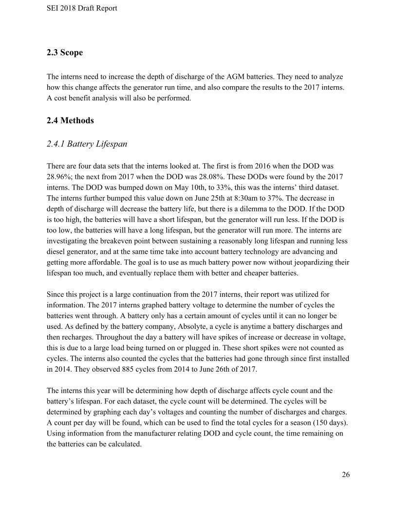
SEI 2018 Draft Report
2.3 Scope The interns need to increase the depth of discharge of the AGM batteries. They need to analyze how this change affects the generator run time, and also compare the results to the 2017 interns. A cost benefit analysis will also be performed. 2.4 Methods 2.4.1 Battery Lifespan There are four data sets that the interns looked at. The first is from 2016 when the DOD was 28.96%; the next from 2017 when the DOD was 28.08%. These DODs were found by the 2017 interns. The DOD was bumped down on May 10th, to 33%, this was the interns’ third dataset. The interns further bumped this value down on June 25th at 8:30am to 37%. The decrease in depth of discharge will decrease the battery life, but there is a dilemma to the DOD. If the DOD is too high, the batteries will have a short lifespan, but the generator will run less. If the DOD is too low, the batteries will have a long lifespan, but the generator will run more. The interns are investigating the breakeven point between sustaining a reasonably long lifespan and running less diesel generator, and at the same time take into account battery technology are advancing and getting more affordable. The goal is to use as much battery power now without jeopardizing their lifespan too much, and eventually replace them with better and cheaper batteries. Since this project is a large continuation from the 2017 interns, their report was utilized for information. The 2017 interns graphed battery voltage to determine the number of cycles the batteries went through. A battery only has a certain amount of cycles until it can no longer be used. As defined by the battery company, Absolyte, a cycle is anytime a battery discharges and then recharges. Throughout the day a battery will have spikes of increase or decrease in voltage, this is due to a large load being turned on or plugged in. These short spikes were not counted as cycles. The interns also counted the cycles that the batteries had gone through since first installed in 2014. They observed 885 cycles from 2014 to June 26th of 2017. The interns this year will be determining how depth of discharge affects cycle count and the battery’s lifespan. For each dataset, the cycle count will be determined. The cycles will be determined by graphing each day’s voltages and counting the number of discharges and charges. A count per day will be found, which can be used to find the total cycles for a season (150 days). Using information from the manufacturer relating DOD and cycle count, the time remaining on the batteries can be calculated.
26

SEI 2018 Draft Report
2.4.2. Generator Runtime For each DOD, the generator runtime should theoretically be decreasing as the DOD increases, as more battery power is used instead of running the diesel generator to provide the equivalent amount of energy. Although the DOD does have an effect on generator run time, other factors such as weather do as well. For example if there is no solar irradiance during the day, then the generator run time will be large regardless of the DOD since the batteries are not fully charged in the first place. On the other end of the spectrum, if it’s an ideal solar day and windy at night, the generator will run less regardless of DOD. Therefore two days of different DODs are not comparable without at least some consideration of the weather conditions on those days. In order to correct for these weather differences, two values were calculated. The first is an average over many days of the generator runtime. The other value is the percentage of the whole island load that the generator has to support each day. This value will allow the interns to better compare between DODs. The values for generator run time were from the data logs that the island engineers record each morning, and the percentages were calculated from values form the ComBox system showed to the interns by Alex Brickett. The logs were documented for each year, except for 2016, so the interns used the ComBox data for the generator run time. 2.5 Results and Analysis 2.5.1. Battery Cycles Since the interns last year determined the number of cycles for a DOD of 30% until June 26th of 2017, there was still several months in the summer season for the batteries to cycle. To determine the number of cycles currently on the batteries, the interns calculated the number of cycles in the 2017 season, and also the number of cycles up until July 9th 2018, when the interns stopped collecting data. The 2017 Shoals’ summer season ended on September 10th, so the batteries were used for 76 more days. The interns had the cycles per day as 1.143 for the 2017 summer season. When rounding up, there were 87 more cycles on the batteries at the end of the season. This season started off with 972 cycles on the batteries. The interns counted the cycles until July 9th 2018 and got 92 cycles. Which means that as of July 9th 2018 there are 1,064 cycles used on the batteries.
27
SEI 2018 Draft Report
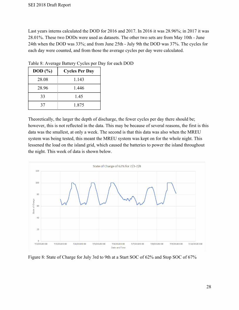
Last years interns calculated the DOD for 2016 and 2017. In 2016 it was 28.96%; in 2017 it was 28.01%. These two DODs were used as datasets. The other two sets are from May 10th - June 24th when the DOD was 33%; and from June 25th - July 9th the DOD was 37%. The cycles for each day were counted, and from those the average cycles per day were calculated. Table 8: Average Battery Cycles per Day for each DOD
DOD (%) Cycles Per Day
28.08 1.143
28.96 1.446
33 1.45
37 1.875
Theoretically, the larger the depth of discharge, the fewer cycles per day there should be; however, this is not reflected in the data. This may be because of several reasons, the first is this data was the smallest, at only a week. The second is that this data was also when the MREU system was being tested, this meant the MREU system was kept on for the whole night. This lessened the load on the island grid, which caused the batteries to power the island throughout the night. This week of data is shown below.
Figure 8: State of Charge for July 3rd to 9th at a Start SOC of 62% and Stop SOC of 67%
28

SEI 2018 Draft Report
To calculate the lifespan left on the batteries, the interns need to know not only know the cycles per day, but also how many cycles these AGM batteries have at certain DODs. A graph comparing the DOD to the battery lifespan was found from the battery’s company, Absolyte.
Figure 9: Lifespan related to Depth of Discharge To calculate the seasons left, the cycles left were divided by the number of cycles per day and the number of days in a season. 150 days a season was used as a safe estimate. Table 9: Graph showing relationship between DOD and Lifespan
DOD (%) Total Cycles Cycles Left Seasons Left
28.08 4100 3036 17.71
28.96 4050 2986 13.27
33 3800 2736 12.58
37 3600 2536 9.02
2.5.3. Generator Run Time The generator run time was calculated and averaged for each of the datasets. The percentage of island load the generator takes each day is the percentage of the island load that runs on non-renewable energy. This value was calculated by dividing the the total generator load by the total island load.
29

SEI 2018 Draft Report
Table 10: Percentage of Island Load Relying on Non-Renewable Energy and Average Generator Run Time
DOD (%) Percentage of Island Load Generator Takes
each Day Generator Run Time Per Day
(hours)
28.08 44.24 7.7
28.96 44.19 6.76
33 41.1 5.95
37 36.7 5.4
2.5.4 Cost Analysis There are two components that go into the cost analysis. The first is the money in diesel gas spent; the second is how much it costs to replace the batteries. 2.5.4.1 Diesel Cost SML has two 27kW-power diesel generators (model: Caterpillar D30-10) and a 65kW-power diesel generator for different purposes. Over the years, only one 27kW generator is in active use when the battery power from clean energy sources are depleted for the day. The 27kW generator uses 2.6 gal of diesel per hour when running. The 2.6 gallons/hour is from the 27kW generator specifications; however, this value is only when the generator is running at peak power, which it does not often do on the island. Since the generator only runs at about 60% of its maximum power, only 1.56 gallons/hour was used. Utilizing the average generator run time for each DOD, the interns could calculated the gallons used in a season. 150 days as a season were used as a safe estimate. The current price of a gallon of diesel, $2.70, in Portsmouth was utilized. Table 11. Costs of Generator Diesel for various Depth of Discharge
DOD (%) Generator Run Time (Hrs) Gallons Used (gal) Total Cost ($)
28.08 7.7 1801.8 4864.86
28.96 6.76 1581.84 4270.968
33 5.95 1392.3 3759.21
37 5.4 1263.6 3411.72
30

SEI 2018 Draft Report
2.5.4.2 Battery Replacement Cost In order to find the most cost effective method, the cost of diesel was weighed against the cost of replacing the batteries. The batteries in the ECB are lead acid batteries, which have been the leading battery for years; however, lithium ion batteries are becoming more common. Due to amount of battery storage, the lifespan, and the continuing research into these batteries, the interns decided that if the ECB batteries are replaced, they should be with lithium ion batteries. The current ECB lead acid batteries cost Shoals $100,000; however, lithium ion batteries are also getting cheaper. The current cost for a kWh is $209, and it is projected to get even cheaper, according to Bloomberg New Energy Finance Analyst, James Frith. The AGM batteries in the ECB is 300 kWh, which would be $62,700 if they were replaced with Lithium Batteries. In the below chart, the smallest decrease in cost was 7%.
Figure 10: Decline in Cost of Lithium Ion Batteries. Graph from a Bloomberg New Energy Finance survey Two predictions were calculated, the first prediction assumed that the price of batteries would stay the same, to get a safe estimate. The second is if the batteries decreased in 2% each year, since the chart above predicts the batteries to decrease in price by more than 2%, so this is again a safe estimate. The two predictions were made to get a more accurate representation of how much it will cost to replace the batteries, as the decrease in battery cost is not definite. The total cost was shown after 5 seasons to show how the cost of diesel gas adds up. The total cost after 9,
31

SEI 2018 Draft Report
12, 13, and 17 seasons were shown as that is how long each battery will last at the corresponding depth of discharge. Since the batteries are replaced with lithium ion ones, the allowable DOD will change as well as the generator runtime. The total diesel cost will be different, so after the batteries are replaced an “N/A” is written for the total cost. Table 12: Battery Cost Estimate Assuming the Cost of Lithium Ion Batteries Stay the Same
DOD (%)
Total Cost after 5 Seasons ($)
Total Cost after 9 Seasons ($)
Total Cost after 12 Seasons ($)
Total Cost after 13 Seasons ($)
Total Cost after 17 Seasons ($)
28.08 24,324.30 43,783.74 58,378.32 63,243.18 149,902.62
28.96 21,354.84 38,438.71 51,251.62 118,222.58 N/A
33 18,796.05 33,832.89 107,810.52 N/A N/A
37 17,058.60 97,905.48 N/A N/A N/A
Table 13: Battery Cost Estimate Assuming the Cost of Lithium Ion Batteries Decrease by 2% each Year
DOD (%)
Total Cost after 5 Seasons ($)
Total Cost after 9 Seasons ($)
Total Cost after 12 Seasons ($)
Total Cost after 13 Seasons ($)
Total Cost after 17 Seasons ($)
28.08 24,324.30 43,783.74 58,378.32 63,243.18 130,369.04
28.96 21,354.84 38,438.71 51,251.62 103,740.29 N/A
33 18,796.05 33,832.89 94,312.26 N/A N/A
37 17,058.60 86,733.33 N/A N/A N/A According to Mike Rosen and Ross Hansen, Shoals should get about 10 years left on the batteries, so the 37% DOD is not feasible as they only have 9 seasons left, and 28.08% as well as it has too many seasons left. The 33% has slightly less than 13 seasons, and the 28.96% DOD has slightly more than 13 seasons. If the batteries have a DOD of 33%, then they will have to be replaced after 12 years, spending $137,884.20 in total diesel gas and battery replacements, utilizing the safe estimate that price per kWh will stay stagnant. If the batteries have a DOD of 28.96%, then they will have to be replaced after 13 years, spending $155,237.64. If priced per year 33% DOD costs $11,490.35 and a 28.96% DOD costs $11,941.36. The most cost efficient choices for each timespan were colored in red, and since the batteries want to be kept for about 10 more years, a DOD of 33% is most cost and lifespan efficient.
32

SEI 2018 Draft Report
2.6 Conclusions and Recommendations The interns came to the island on June 18th, and changed the DOD to 37% on June 25th. However, The first week the DOD was changed there was an issue with the system. The voltage was the factor that was causing the system to switch to the generator, not the state of charge. Ross Hansen and Mike Rosen fixed this problem on July 1st. Therefore, the data set for 37% DOD was only a week long, the interns would have preferred to have more days to collect data at that depth of discharge. The MREU system was in the process of experimentation of being integrated into the island grid, so the results of the interns’ study may change after the salt water pump is completely taken off the grid. Another evaluation on the depth of discharge should be done to analyze what effect the fully automated MREU system has on the green grid AGM batteries. Based on diesel and battery cost, the interns recommend to leave the batteries at 33% DOD for the summer season. The diesel cost is also dependent on time, so if there is a point in the future where cost spikes up a significant amount, the DOD may need to be increased. The interns also believe that the lithium ion batteries should replace the AGM batteries, due to a longer lifespan and greater allowable discharges. 2.7 References Alex Brickett, UNH Project Manager/former SML Island Engineer Parkin, Brian. “CATL's German Battery Plant Lifts Prospect of Electric Car Push.” Bloomberg.com, Bloomberg, 9 July 2018, www.bloomberg.com/news/articles/2018-07-09/catl-s-german-battery-plant-lifts-prospect-of-electric-car-push. Zart, Nicolas. “Batteries Keep On Getting Cheaper.” CleanTechnica, 11 Dec. 2017, cleantechnica.com/2017/12/11/batteries-keep-getting-cheaper/ O'Connor, Joe. “Battery Showdown: Lead-Acid vs. Lithium-Ion – Solar Micro Grid – Medium.” Medium, Augmenting Humanity, 23 Jan. 2017, medium.com/solar-microgrid/battery-showdown-lead-acid-vs-lithium-ion-1d37a19982 https://www.gasbuddy.com/GasPrices/New%20Hampshire/Portsmouth
33
SEI 2018 Draft Report
Assignment 3: Analysis of SML’s Solar Arrays Project Leads: Gabby Peralta and Laurel He 3.1 Background SML installed its first solar array in 2007 (4.5 kilowatts) on Dorms 2 and 3, the Dorm 3 PV panels are older models and were previously in storage for many years before being donated to Shoals. Today, SML has 331 solar panels, with ground and roof arrays installed throughout the northern side of the island in 2014. A new donated system was also installed on Kingsbury House in spring 2018. SML also maintains a solar array on White Island for energy production to support its Tern Restoration Program. Although solar arrays can last up to 30 years, there are many factors that can affect the efficiency, such as temperature, age, upkeep, orientation, tilt angle and in the Island’s case, gull pucky. The SEIs calculated the efficiency of the solar arrays, while taking into account all these factors. The interns also evaluated the maintenance and output of all of these solar arrays to gauge the current quality. Using the nameplate data, the maximum efficiency output was determined, and measuring the voltage and current output from the combiner box, the actual output was calculated for each array. The wiring, setup, and bolts were also checked. 3.2 Purpose Shoals Marine Lab has installed multiple solar arrays throughout the years, and the panels may not be at peak performance over the years since installation. Data should be taken to determine the actual output, and compare that to the nameplate values. Factors affecting the output efficiency should be considered and quantified. All of the arrays need to be inspected to make sure the mechanical and electrical parts are running smoothly. 3.3 Scope The interns needed to not only check to see if the electrical and mechanical components of the solar arrays were in order, but also the energy output. Using the current flowing across the panels and their voltage, the interns needed to determine the actual power the solar arrays are outputting, and then compare that to the nameplate data. The temperature, tilt, and irradiance will also be determined to further determine the efficiency of the panels.
34

SEI 2018 Draft Report
3.4 Methods 3.4.1 Map of the Solar Arrays Since the interns needed to work with over 90 kW of solar panels, they mapped out all of the ground and roof arrays to keep track. A naming convention was also created for the southern based arrays as it was hard to keep track of the 13 arrays. These arrays were named corresponding to its charge controller. A schematic is represented below.
Figure 11: Layout and Numbering of the Northern Solar Arrays The arrays in the southern part of the island did not have the same ease of naming style, as the dorm panels are connected to the radar tower, and the Kingsbury House has its own system. The solar panels were counted on the dorms, and for K-House, the panels were identified the same way as the others. Each pair of the 14 arrays correspond to its own charge controller.
35

SEI 2018 Draft Report
Figure 12: Layout of Southern Solar Arrays 3.4.2 Power Output The solar panels produce DC power, which is then converted to usable AC power by the inverters. The most common module efficiency of the solar panels reported by the manufacturers is about 15%, meaning the panels only produce power from 15% of the incoming solar irradiance. Solar panels have their best performance under very specific conditions, and are very sensitive to changes in these conditions. Several other factors affect the efficiency of solar panels, including temperature, position and tilt angles, time since installation, shading and maintenance. Manufacturer specs include graphs detailing the efficiency loss as a function of time. The maximum efficiency temperature for these solar panels are usually 25°C or 77°F, and heating of the solar panels in the summer season will reduce the efficiency. On Appledore island in particular, shading comes in coverage of gull pucky as the island houses hundreds of seagulls. To find the working efficiencies of the solar panels, the interns calculated the efficiency loss taking into account all these factors in order to obtain a more accurate and realistic depiction. These data were then compared to the actual output of the panels to see how they are performing compared to how the panels should be theoretically performing.
36

SEI 2018 Draft Report
3.4.2.1 Actual Power Output To get get a measure of how well the current solar panels are performing, the interns needed both the actual output, and the maximum efficiency output. To get the actual output the interns had Ross Hansen’s help. A multimeter was used to get the voltage and current of each string in each solar array. A combiner box held the current and voltage wires for each string of the array. Ross used the multimeter to get the current and voltage, while the interns recorded the results. The numbers would jump around, since the solar energy coming in is not completely constant, so the number that was in between the high and low values was used. All of the ground arrays were evaluated and the arrays on the roof of the ECB, Pole Barn, Fuel Tank, Dorms 2 and 3, and K-House. The interns utilized the following equation to get the actual power output, where P is power, I is current, and V is voltage:
P=I*V Eqn. 1 The solar panels were also evaluated a day after a large rain storm, so the panels had less gull pucky than usual. This means the the gull pucky obstructing the efficiency can be thought of as less of an issue than if the panels were covered in gull pucky. Professor Martin Wosnik of University of New Hampshire was contacted for further analysis of the solar panels. He responded with an equation to calculate the actual working efficiency.
Eqn. 2
Where Pmax is the maximum power output, Ac is the area of the array, and E is the irradiance measured from the pyranometer. 3.4.2.2 Maximum Efficiency Power Output Getting the maximum efficiency power output required more calculations. Each solar company’s speculations had specific currents and voltages for each array. For each string in each array, it had to be determined if they were in series or parallel. Using basic rules of circuits, the voltage and current were found. Since all the string were in series, the open circuit voltage (Voc) was added. Each string was in parallel with each other, so the short circuit currents (Isc) were added. So the equations below were done to each array, as long as the panels were in series, and the strings were in parallel.
37

SEI 2018 Draft Report
# of Panels per String*Voc = Voltage of Array (Eqn. 3) # of Strings per Array*Isc = Current of Array (Eqn. 4) These voltages and currents were used to solve for the maximum power output, the same way as equation 1. This value is the power output when the solar array is running at Standard Test Conditions (STC), which is 25℃, 1000 W/m2, and air mass 1.5, and since the solar arrays are not running at STC, the interns did some efficiency corrections. UNH Professor Martin Wosnik said the interns did not have to correct for air mass, since the interns were measuring the solar panels directly how they were performing, not stimulating an environment. The STC temperature is 25℃, and solar panels get less efficient as they heat up. Using an infrared thermometer, the temperatures of the solar panels was found. The solar panels ranged from about 114℉ to about 130 ℉, which is 45.56℃ and and 54.4℃, respectively. These temperatures are higher than 25℃, which means the efficiency needs to be corrected.
Lost Efficiency from Temperature = (Solar Panel Temp. - 25℃)*Temp. Coeff. (Eqn. 5) The temperature coefficient is a value that differs between solar panel companies, which determines how much the efficiency will decrease per one degree of temperature increase. The lost efficiency was factored in using the equations:
Adjusted Efficiency = Original Efficiency of Panel *(1- Lost Efficiency from Temperature) Eqn. 6 The infrared temperature sensor was used on both the lower and upper rows, as it varied which panels were more in the sun. This produced temperatures that were different between the two rows. Three readings on each row were taken, and an average of those values were calculated. In order to get a higher and lower temperature efficiency loss value, two values for each array were calculated. The STC for irradiance is 1000 W/m2, but the actual irradiance varies based on the time of day and the intensity of the sun. The interns collected data from the solar panels from about 9:30-11:30 am, and therefore the irradiance was averaged over those hours. Below are some of the values from the pyranometer data. At first the pyranometer data on the island was utilized; however after talking with Professor Wosnik, it was made clear that due to the the pyranometer not being cleaned and calibrated, the irradiance data was off. A website, pveducation.org, was provided by Professor Wosnik as a way to get the irradiance.
38

SEI 2018 Draft Report
Table 14: Pyranometer for the Time when the Interns Collected Solar Array Data
Hour Irradiance (kW/m2)
9.38 0.996
9.50 1.001
9.63 1.006
9.75 1.010
9.88 1.015
10.00 1.018
10.13 1.022
10.25 1.025
10.38 1.028
10.50 1.031
10.63 1.034
10.75 1.036
10.88 1.038
11.00 1.040
11.13 1.041
11.25 1.043
11.38 1.044
11.50 1.045
The pyranometer data are used to determine the maximum power available for the solar arrays to absorb and convert to electricity, which can then be compared to the actual power the solar arrays produce. In order to get the total power the solar panels can produce, the irradiance has to be multiplied by the total area of the solar arrays. However, this value is not the power output since solar panels have efficiencies of about 15%. Once the losses have been accounted for, then the temperature losses can also be included using Eqn 6. This value is the optimal solar power output at the current irradiances and temperature.
39

SEI 2018 Draft Report
3.4.3 Evaluating State of All Solar Panels Solar panels are usually low maintenance. However, here on the island gull pucky is constantly covering the panels and it requires manpower to clean them up regularly. This is a problem as solar panels especially the higher quality monocrystalline solar panels are very sensitive to shading, and SML has been relying on rainwater to washdown the pucky. Previous interns have considered installing hydrophobic coating on solar panels, but they concluded it might not be a cost effective solution. Another big part of maintenance is checking the bolts on the arrays and the wiring. The interns used a torque wrench to tighten the screws. Arrays 3-6 and 10-13 all had dry bolts which needed to be tightened to 10.5 foot-pounds. The torque wrench was calibrated to this exact value, and automatically clicked when the 10.5 ft-lb force was reached. The ground arrays were the only arrays where the bolts were tightened, since there is not as safe a footing on the roof arrays. Arrays 10-13 are higher up than arrays 3-6, so the interns used a ladder; however, the interns were unable to reach the second row from the top of the ground arrays past the pole barn.
Figure 13: Tightening Bolts
40

SEI 2018 Draft Report
3.4.4 Tilt Angle and Orientation In order to capture the maximum amount of solar radiance, the amount of tilt is approximately the latitude angle of the site facing 15 degrees due South. Empirically, if the tilt angle of the solar arrays is within 15% of the latitude angle, a 5% or less reduction in annual power output can be achieved. The interns used a Silva compass to measure the tilt angles of the solar arrays to see if the solar arrays are tilted to reach their best performance. When laying the compass on its side directly against the solar panels, the dip angle can be read from the clinometer. The interns took direct measurements on the ground mounted solar panels. Similarly, the exact positions of the ground mounted solar arrays can be measured by placing the Silva compass directly on the panels and measure the plunge angle. The roof mounted ones can be estimated by positioning the compass approximately to the direction they are facing and take several readings to minimize the uncertainty.
Figure 14: Tilt Angle (left) measured as Dip; Array Position (right) measured as Plunge 3.5 Results and Analysis 3.5.1. Actual versus Maximum Working Efficiency The theoretical maximum power output are computed based on the manufacturer data for the different models of solar panels used on Appledore island. For each series of solar panel, an open circuit voltage (Voc) and a short circuit current (Isc) are given on the manufacturer specs
41
SEI 2018 Draft Report
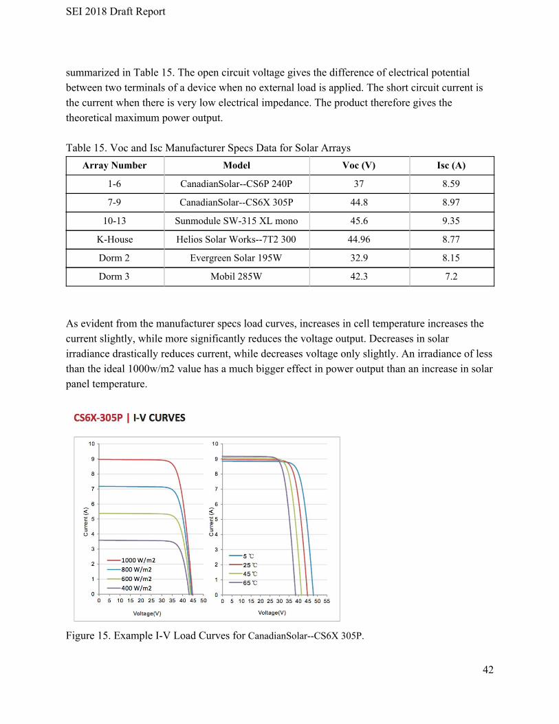
summarized in Table 15. The open circuit voltage gives the difference of electrical potential between two terminals of a device when no external load is applied. The short circuit current is the current when there is very low electrical impedance. The product therefore gives the theoretical maximum power output. Table 15. Voc and Isc Manufacturer Specs Data for Solar Arrays
Array Number Model Voc (V) Isc (A)
1-6 CanadianSolar--CS6P 240P 37 8.59
7-9 CanadianSolar--CS6X 305P 44.8 8.97
10-13 Sunmodule SW-315 XL mono 45.6 9.35
K-House Helios Solar Works--7T2 300 44.96 8.77
Dorm 2 Evergreen Solar 195W 32.9 8.15
Dorm 3 Mobil 285W 42.3 7.2
As evident from the manufacturer specs load curves, increases in cell temperature increases the current slightly, while more significantly reduces the voltage output. Decreases in solar irradiance drastically reduces current, while decreases voltage only slightly. An irradiance of less than the ideal 1000w/m2 value has a much bigger effect in power output than an increase in solar panel temperature.
Figure 15. Example I-V Load Curves for CanadianSolar--CS6X 305P.
42

SEI 2018 Draft Report
3.5.1.1. Actual Outputs The interns collected the voltage and current of each string of each array with Ross Hansen. Each “string” is a row of solar panels connected in series, and each “string” is in parallel with each other. Table 16: Current and Voltage of the Southern Arrays
43

SEI 2018 Draft Report
Table 17: Current and Voltage for Northern Arrays
The dorms’ arrays were set up slightly different than the northern arrays. For Dorm 2, there were combiner boxes on the roof, which combined strings 1 and 2 before they reached the measuring point, which is why the current is larger. Dorm 3 did not have the corresponding charge controllers listed, so the values were determined by the combiner boxes. Using equation 1, the actual outputs were calculated for each solar array found. Table 18: Actual Power Output of Southern Arrays
Southern Solar Array Locations Array Number Power Output [W]
ECB Roof 1 3872.40
ECB Roof 2 3688.49
ECB Ground 3 3734.51
ECB Ground 4 3561.30
ECB Ground 5 3692.94
ECB Ground 6 2874.70
Fuel Tank Building 7 2610.85
Pole Barn Roof 8 2666.38
Pole Barn Roof 9 1905.70
Ground Mount Past Pole Barn 10 1659.44
Ground Mount Past Pole Barn 11 1926.00
Ground Mount Past Pole Barn 12 2003.68
Ground Mount Past Pole Barn 13 1620.76
44

SEI 2018 Draft Report
Table 19: Actual Power Output of Northern Arrays
Northern Solar Array Locations Array Number Power Output (W)
Dorm 2 N/A 1411.02
Dorm 3 N/A 101.38
K-House 1 514.30
K-House 2 294.36
K-House 3 112.36
K-House 4 56.18
K-House 5 608.58
K-House 6 0.00
K-House 7 414.60
The power output for K-House array 6 was zero since the current reading was zero. It is possible that the current was a non-zero value, but too small to be picked up by the ammeter. To calculate the efficiency, the pyranometer data must be averaged. The average irradiance was 1024 W/m2. Using eqn 2 the actual efficiencies can be calculated. Table 20: Actual Efficiencies of Northern Arrays
Northern Solar Array Locations Array
Number Efficiency
Dorm 2 N/A 7.08%
Dorm 3 N/A 0.48%
K-House 1 1.83%
K-House 2 1.05%
K-House 3 0.40%
K-House 4 0.20%
K-House 5 2.17%
K-House 6 0.00%
K-House 7 1.48%
45

SEI 2018 Draft Report
Table 21: Actual Efficiencies of Southern Arrays
Southern Solar Array Locations Array
Number Efficiency
ECB Roof 1 13.06%
ECB Roof 2 12.44%
ECB Ground 3 12.60%
ECB Ground 4 12.01%
ECB Ground 5 12.46%
ECB Ground 6 9.70%
Fuel Tank Building 7 5.54%
Pole Barn Roof 8 9.69%
Pole Barn Roof 9 6.93%
Ground Mount Past Pole Barn 10 5.89%
Ground Mount Past Pole Barn 11 6.84%
Ground Mount Past Pole Barn 12 7.11%
Ground Mount Past Pole Barn 13 5.75%
3.5.1.2. Maximum Efficiency Calculation The maximum power based on the manufacturer values was calculated. The max power was found by using equation 1. Table 22: Max Power Per Location
46

SEI 2018 Draft Report
A solar panel efficiency of 15% means that only 15% of the solar energy input is converted to electricity output. The efficiency value is different for each solar panel manufacturer. Table 23: Efficiencies of Solar Arrays based on Manufacturer
For Dorm 3, the manufacturer did not specify the Efficiency, so 15% was used as a safe value. Another large inefficiency the interns found was the increase in temperature of the solar panels. A low and high temperature was recorded as the arrays were different temperatures at different points. Both high and low are calculated to get an idea of the lowest and highest efficiency lost. Table 24: Temperature of each Array and the Efficiency Lost from Increase Temperature
47

SEI 2018 Draft Report
This efficiency loss was subtracted from the inherited efficiency of the panels. Table 25: Corrected Efficiency from Temperature Increase for Northern Arrays
Array Number
Higher Efficiency Temperature Correction
Lower Efficiency Temperature Correction
1 0.143 0.140
2 0.143 0.140
3 0.144 0.142
4 0.144 0.140
5 0.144 0.140
6 0.142 0.142
7 0.144 0.141
8 0.144 0.141
9 0.144 0.141
10 0.146 0.144
11 0.145 0.143
12 0.146 0.141
13 0.148 0.143
Since all of the Southern arrays are on roofs, the interns were unable to get temperature readings. The interns used the average temperature of the ground solar panels. Table 26: Corrected Efficiency from Temperature Increase for Southern Arrays
Array Location
Higher Efficiency Temperature Correction
Lower Efficiency Temperature Correction
Dorm 2 0.136 0.133
Dorm 3 0.136 0.133
K-House 0.139 0.136
48

SEI 2018 Draft Report
3.5.2 Tilt Angle and Orientation Table 27. Solar Array Orientations and Tilt Angles
The interns used the Silva compass to check the orientations of the solar arrays. The solar arrays have the best performance when they are facing due South or in the 15 degree range due South (180°±15°). The solar arrays in the ECB area have the best orientation. Because the interns could only do direct measurements on the ground mounted solar arrays, there could be uncertainty in the estimation for the roof mounted ones. At the same time, roof mounted solar array installations are limited by the orientation of the existing buildings. Because they are in the SE and NW orientation instead of facing due South, the PV panels on K-House reach peak performance at different times than the rest of solar arrays. The intention is to try spreading out solar capture throughout the day to have a consistent high battery power. Generally, the amount of tilt should be approximately equal to the latitude angle (within 15%) of the site to capture the maximum amount of solar radiance. Appledore island has a latitude of 42.9891° N, and 15% less than that latitude angle is 36.5407°. At the same time, seasonal position of the sun should be taken into account. The interns used Foresthillweather.com to generate the ideal array tilt angle for each month and compared to the actual measurements. The interns measured the tilt angles for the ground mounted solar arrays, as only those are accessible to lay down the compass directly on the panels. Rightnow, the tilt angle is about 20 degrees and is optimal in the May/June/July season. Because the island is only open from May to the end of August, there’s little need to change the array tilt constantly. The interns expect an annual energy production reduction of 5% or lower due to tilt angle and position. Based on a rough analysis on the positions and tilt angles of the solar arrays installed around Appledore island, the interns concluded that the panels are performing very close to their best performance.
49

SEI 2018 Draft Report
Table 28. Ideal Solar Array Orientations and Tilt Angles at Latitude 43°N
Using an additional 5% reduction in efficiency, the following table summarizes the efficiency of the solar panels after subtracting temperature and tilt angle reduction from theoretical maximum efficiency. Table 28. Range of Temperature Correction for Northern Solar Arrays
Array Number Higher Efficiency Temperature
Correction Lower Efficiency Temperature
Correction
1 0.136 0.133
2 0.136 0.133
3 0.136 0.135
4 0.136 0.133
5 0.137 0.133
6 0.135 0.134
7 0.136 0.134
8 0.136 0.134
9 0.136 0.134
10 0.139 0.137
11 0.138 0.136
12 0.138 0.134
13 0.140 0.136
50
SEI 2018 Draft Report
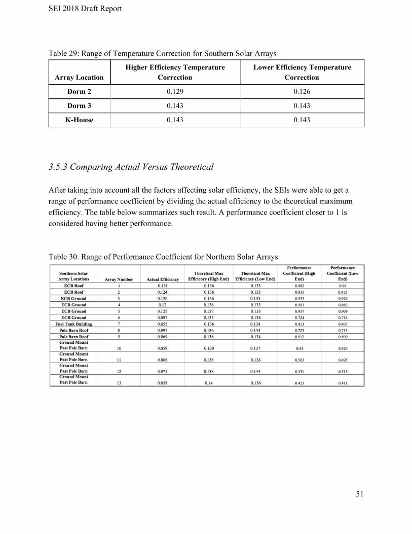
Table 29: Range of Temperature Correction for Southern Solar Arrays
Array Location Higher Efficiency Temperature
Correction Lower Efficiency Temperature
Correction
Dorm 2 0.129 0.126
Dorm 3 0.143 0.143
K-House 0.143 0.143
3.5.3 Comparing Actual Versus Theoretical After taking into account all the factors affecting solar efficiency, the SEIs were able to get a range of performance coefficient by dividing the actual efficiency to the theoretical maximum efficiency. The table below summarizes such result. A performance coefficient closer to 1 is considered having better performance. Table 30. Range of Performance Coefficient for Northern Solar Arrays
51

SEI 2018 Draft Report
Table 31. Range of Performance Coefficient for Southern Solar Arrays
Table 32. Summary of Average Efficiency, Performance Coefficient and PV Panel Type
From Table 32., solar arrays on the ECB roof and the ground mounted ones next to the Energy Conservation Building have the best performance. The solar arrays on the pole barn roof, the fuel tank building and the ground mounted ones past pole barn perform about equally well. The solar arrays on dorm 2 perform as well as those in the pole barn area. However, the solar arrays on dorm 3 and on K-House do not perform nearly as well. Considering the PV panels have been installed for 11 years on dorm 3 and the model and panels themselves are older, it might explain the low performance. The K-House has high quality monocrystalline solar panels, which have only been installed for several months, should have much better performance than calculated. This is explained by looking into the following power output data from charge controllers in K-House. Monocrystalline solar panels performs better overall than polycrystalline ones, but this is contrary to the trend we see in this table. This is mostly like because monocrystalline panels
52

SEI 2018 Draft Report
are sensitive to unclean panels like dust and shades. Because gull pucky is a constant problem to these panels, polycrystalline panels seem to have outperformed them.
Figure 16: Graph for each Charge Controller of K-House for June 29th The interns took these measurements on June 29th at around 11:30 for K-House. At this point, charge controller #6 is producing 0W; however at about 8am it was producing the most wattage. This means the orientation of charge controller #6 is most efficient in the early morning, and not when the interns measured it. Charge controllers 1, 2, 3 and 4 are connected to solar panels on the NW, with 4 connected to panels at a lower angle. They generally perform best in the late afternoon and early evening. Charge controllers 5, 6 and 7 are connected to solar panels on the roof facing SE, and perform best early in the morning. This is exactly the intention of installation in the first place, trying to spread out the peak performance time throughout the day. 3.5.4 Solar Array Corrections The ground arrays’ conditions haven’t been checked since 2014 installation. A torque wrench was used to tighten the dry bolts on the ground arrays. Most of the bolts on the arrays by the ECB needed a few turns to tighten, which was looser than expected. A ladder was utilized to reach the higher bolts. The bolts on the ground mount arrays past the pole barn needed much less tightening. Although many were at the recommended torque value to begin with, there were also
53

SEI 2018 Draft Report
some bolts that needed tightening. The distribution between tight and loose bolts was random, so the interns checked all the bolts that they could safely reach. This loosening was probably caused by vibration caused by wind and by tightening the dry bolts, it helps lessen the friction between parts that might reduce efficiency. Several of the combiner boxes also needed some repairs. The box on the Pole Barn needed a clip fixed as it was not closing. The box on Dorm 2 was rusted and may need to be examined. The first box for K-House also had a leak in the back, so water was running through the wires. 3.6 Conclusions and Recommendations The SEIs measured and calculated the actual operating efficiency of all the solar arrays on Appledore island. They compared the results to theoretical maximum efficiency provided by PV panel manufacturers, and assigned to a performance coefficient to solar arrays at each location. According to this rating, the solar arrays in the Northern part of the island has the best performance. The interns also attempted to offer suggestions to each factor affecting solar efficiency. Position, orientation and tilt angle wise, the majority of the solar arrays seem to be performing with maximum efficiency since they face directly due South. Since Shoals Marine Lab only operates during the summer month, having a tilt angle of about 20° facing South is optimal. SML does not have to worry about changing the tilt angle as the incoming solar direction changes throughout the season. As the K-House has set a good example of utilizing existing houses to maximize solar power production throughout the day, similar constructions could be done on other houses. Future studies could look into the feasibility of moving older, less efficient panels to face directly due South, and install new, efficient panels to existing rooftops of a lesser desirable orientation in order to get the maximum efficiency out of every panel. The effect of shading in the form of gull pucky is hard to quantify, since this factor is highly variable. The problem could be intensified by more gulls residing at one location more frequently, or lessened by having a rain event. The previous interns considered installing a hydrophobic coating on the panels so that the pucky could be washed down more easily by the rain, but they concluded this might not be the most cost efficient solution. Overheating of the solar panel is a major contributing factor to reduced efficiency, especially in the summer seasons when the solar arrays are heavily relied on. Technology like thermosiphon self-cooling fin system (TSC) and photovoltaic powered self-cooling fin system (PVSC) exist,
54

SEI 2018 Draft Report
but would likely be costly to SML. Since the lab only operates in summer, a more economic way is to spray the solar panels with water during the hot days to cool down the panels as well as to clean them from dusts and gull pucky. Freshwater is ideal as nothing gets left behind on the panels once the water evaporates. Rainwater could be collected in buckets to be used in this cleaning and cooling purposes, as it is the cleanest option besides using fresh drinking water. Piping system could be installed on the panels and spray water when needed. It could be taken down in winter when the solar panels are not in use, and to prevent the piping from bursting because of the cold. Also, the overheated panels can be covered by sheets of plywood, which can shield the solar panels from gull pucky at the same time. Regular maintenance is recommended, since the interns found a lot of the dry bolts were loose when tightening with a torque wrench. It is recommended that once every few years the screws should be checked in order to minimize friction in the parts of the solar panels. Wiring should also be checked to make sure no wires are exposed and no water can get into the combiner boxes. 3.7 References Ross Hansen Martin Wosnik, UNH “How to Position Solar Panels to Maximize Efficiency.” Buy Solar Panels | Learn from the Solar Experts, www.wholesalesolar.com/solar-information/solar-panel-efficiency. “Solar Electric Design: PV Array Tilt Angle Calculator.” Foresthill Weather.com - UV Index, Forecast, www.foresthillweather.com/PHP/Conversion/SunCalc2.php. “PVEducation.” Properties of Light | PVEducation, www.pveducation.org/pvcdrom/properties-of-sunlight/calculation-of-solar-insolation.
55
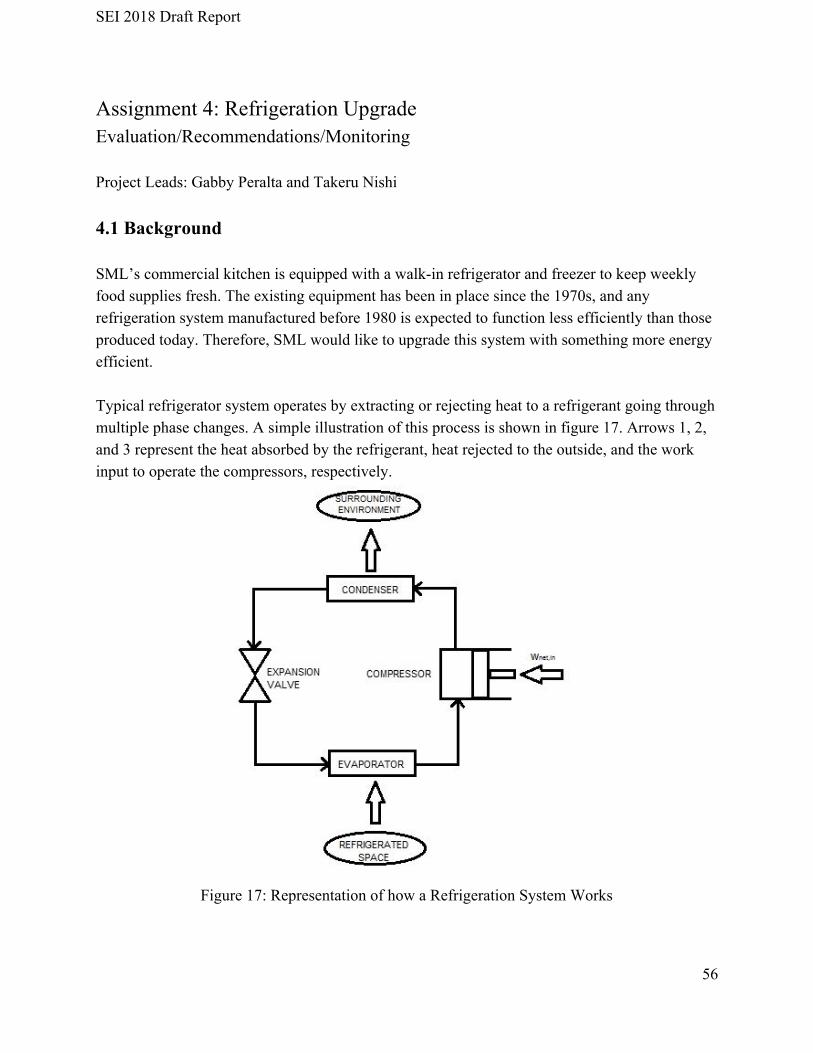
SEI 2018 Draft Report
Assignment 4: Refrigeration Upgrade Evaluation/Recommendations/Monitoring Project Leads: Gabby Peralta and Takeru Nishi 4.1 Background SML’s commercial kitchen is equipped with a walk-in refrigerator and freezer to keep weekly food supplies fresh. The existing equipment has been in place since the 1970s, and any refrigeration system manufactured before 1980 is expected to function less efficiently than those produced today. Therefore, SML would like to upgrade this system with something more energy efficient. Typical refrigerator system operates by extracting or rejecting heat to a refrigerant going through multiple phase changes. A simple illustration of this process is shown in figure 17. Arrows 1, 2, and 3 represent the heat absorbed by the refrigerant, heat rejected to the outside, and the work input to operate the compressors, respectively.
Figure 17: Representation of how a Refrigeration System Works
56

SEI 2018 Draft Report
Each component of the system was monitored for a week using a data collection apparatus supplied by Ross and analysis was performed using a software called Fluke. This program allowed interns to interpret the energy usage of the system. Also, many of the system components, including structural materials and insulation, had not been compiled, so it became necessary to inquire the manufacturer for that information. Another crucial part of refrigeration systems is the refrigerant. Most commercial refrigerants are comprised of halogenated hydrocarbons, meaning it includes elements like bromine, chlorine, and fluorine bonded to carbon. Though these compounds perform effectively in a refrigeration cycle, most are highly damaging to the environment. The most commonly used criteria to determine a compound’s environmental degradative capability are the ozone depletion potential and global warming potential. Ozone depletion potential is a comparative measurement of impact on ozone per unit mass between the test gas and CFC-11 (trichlorofluoromethane), whose ODP is normalized to 1.0. Any numbers higher indicate a greater ability to degrade ozone and values approaching zero indicate lesser ozone degradation. Global warming potential (GWP), on the other hand, is a measure of a gas’ contribution to the greenhouse effect, or the trapping of heat in the atmosphere; like the ODP, these values are comparative to that of CO2. Put simply, a gas with a GWP of 10 is ten times stronger than CO2 in producing the greenhouse effect. It might be assumed that compounds posing a threat to the environment would rate high on both of these scales. This would be an incorrect assumption to make. For a refrigerant like fluoroform (R-23) the ODP is 0, whereas the GWP is upwards of 15000. The main reason for this discrepancy is that hydrofluorocarbons, like R-23, react in lower levels of the atmosphere and are unable to reach the ozone layer. Since many refrigerants were discovered to have high ODP or GWP values, a process of “phasing out” was implemented, where users were encouraged to replace these damaging refrigerants with safer alternatives. Much of this phasing out was enacted as a result of strict legislation. At face value, this may seem like a simple choice to replace a refrigerant, but there are three things one must keep in mind when changing to a new refrigerant: efficiency, difference in ODP and GWP values, and ease of replacement. 4.2 Purpose The walk in refrigerator and freezer were installed in the 1970s, so all the equipment and materials may not be up to date. The interns will determine what components need to be replaced, and what components to add to make the system more efficient.
57

SEI 2018 Draft Report
4.3 Scope The interns must determine how well the refrigerator system is operating after decades of use. They must also give recommendations on how to upgrade the system in a cost effective and energy efficient manner. A schematic will also be made describing how the system works. 4.4 Methods 4.4.1 Efficiencies The refrigerator is a large load for the island, so the interns evaluated the efficiency of the system. Justin Ulrich from Unitil came out to help the interns get and analyze the data from the monitor Ross Hansen had placed on the system weeks before. A data software, Fluke, allowed the interns to record and graph the data. Data for both the freezer and fridge compressor energy usage was available, and also the freezer fans and defroster, and the refrigerator fans. It was observed that of the three evaporator fans in the fridge, only two were spinning, which means that data is lower than if all fans were working. Refrigerators should not be running all day. The compressors should only start working when the temperature fluctuates, so the energy graph should have values of zero at some points. The temperature of the fridge and freezer should also not be fluctuating very often. The defroster should also be only operating when it needs to be. 4.4.2 System Components In order to gain a comprehensive understanding of the current system, knowledge of exact components is necessary. The interns referred to the fridge and freezer nameplates for data such as the refrigerant, operating frequency of the motor, and the make and model. Nameplate data for the compressors of the refrigerator and freezer are compiled in table 33. This information was used to make recommendation on compressor replacements.
58

SEI 2018 Draft Report
Table 33: Nameplate Data of Refrigerator and Freezer
Knowing this data can help the interns decide what components of the existing system are in need of replacement. Of these components, the most easily replaced is the refrigerant, since no mechanical alterations need to be made. Research was done on multiple refrigerant replacements so that an informed recommendation can be made. The model number also has useful information, as each letter or number indicates something about the operating conditions of the compressor. Table 34 lists all the data gathered from this code. Table 34: Defining the Model Number for the Refrigerator and Freezer
59

SEI 2018 Draft Report
The compressors are long out of date, so the “203” part of the refrigerator nameplate, which corresponds to horsepower, was not listed in any available database. In Emerson’s list of nameplate nomenclature, “200” was the closest value that could be translated to horsepower. A horsepower of 2 was used for the refrigerator compressor. Since insulation is one of the materials whose quality degrades over a long period of time, intens gathered data on the type of insulation and its dimensions surrounding the refrigerator to better understand how it may be affecting refrigerator performance. Crown Tonka, the company that manufactured the current system, was contacted with questions about insulation and materials. Fortunately, a response came from the Steve Combs, the engineering manager at Everidge. He was able to provide most of the requested information, stating that the insulation is a two part urethane foam system injected into galvanized steel metal skinned panels. 4.5 Results and Analysis 4.5.1 Energy Usage Ross Hansen placed energy loggers on both the refrigerator and freezer compressors and evaporator fans, and the freezer defroster. These loggers collected data over the span of a week. Table 35 shows the refrigerator energy consumption on the compressor and evaporator fans. Table 35: Energy Consumption for Fridge
The energy consumption by the fridge fans is an underestimate because only 2 of the 3 fans are functional. The third fan appeared to be stuck and unable to rotate.
60

SEI 2018 Draft Report
Table 36: Energy Consumption for Freezer
The average island load is about 270 kWh, so the whole fridge/freezer system makes up about 14% of the island’s load.
Figure 18: Graph of Energy Consumption of the Fridge Compressor over several Hours Justin Ulrich from Unitil came to help the interns understand the fridge data. He said the since the data was varied, characterized by the significant variance in figure 18, it meant the power coming in from the generator was not in phase with the compressor motor. A variable frequency device (VFD) can be used to correct for this.
61

SEI 2018 Draft Report
The temperature of the kitchen, fridge, and freezer was recorded over several days. If temperature changes too often, it could be indicative of cold air escaping from the inside. Figure 19 shows the temperature changes over a ten day span.
Figure 19: Temperatures for Kitchen, Fridge, and Freezer Table 37: Temperature Statistics for the Refrigerator, Freezer, and Kitchen
The fluctuations of the fridge temperature could be explained by the opening and closing of the main door; this would allow for a significant amount of cold air to escape. However, freezer temperature is not set at the desired level. According to the U.S. Food and Drug Administration, freezers should not be set above 0℉, but the current freezer temperature stagnates around 10˚F. This may be an error in the thermostat setting, so a quick adjustment would suffice.
62

SEI 2018 Draft Report
4.5.2 Dimensions The refrigerator system was measured, and a CAD of the system was made.
Figure 20: CAD of the Refrigerator and Freezer System
Table 38: Outside Dimensions of the System Table 39: Inside Fridge Dimensions
Table 40: Freezer Dimensions
63
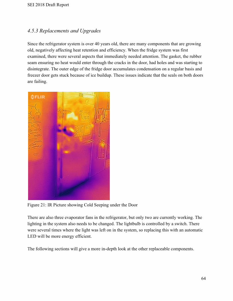
SEI 2018 Draft Report
4.5.3 Replacements and Upgrades Since the refrigerator system is over 40 years old, there are many components that are growing old, negatively affecting heat retention and efficiency. When the fridge system was first examined, there were several aspects that immediately needed attention. The gasket, the rubber seam ensuring no heat would enter through the cracks in the door, had holes and was starting to disintegrate. The outer edge of the fridge door accumulates condensation on a regular basis and freezer door gets stuck because of ice buildup. These issues indicate that the seals on both doors are failing.
Figure 21: IR Picture showing Cold Seeping under the Door There are also three evaporator fans in the refrigerator, but only two are currently working. The lighting in the system also needs to be changed. The lightbulb is controlled by a switch. There were several times where the light was left on in the system, so replacing this with an automatic LED will be more energy efficient. The following sections will give a more in-depth look at the other replaceable components.
64

SEI 2018 Draft Report
4.5.3.1 Refrigerants The walk-in fridge uses R-22 and the freezer uses R-408A, which replaced R-12. R-22 belongs to a group of refrigerants that are being phased out, as explained earlier. Chlorodifluoromethane, R-22’s real name, has a global warming potential of 1760 and an ozone depletion potential of 0.055, both of which are too high by current standards. It is favorable to replace this with another, more environmentally friendly refrigerant. R-408A has a composition of 47% chlorodifluoromethane, 46% 1,1,1-trifluoroethane, and 7% pentafluoroethane. Though this refrigerant was used to replace the banned R-12, its composition is nearly half R-22, meaning its global warming potential is still very high. Recent legislation has forced cutbacks on production and use of refrigerants with high GWP, meaning R-408A will soon be phased out of the market. An issue that may come from this is that the compressors used in Kiggins cannot use the newer, more environmentally friendly refrigerants. With the popularity of cleaner refrigerants like CO2 and propane growing, it is important to know not to mix these with older, outdated halogenated hydrocarbons like R-22. The main reason for this is because the two compounds exhibit different properties, the most notable of which is flammability; halogenated hydrocarbons are not flammable, whereas propane is especially flammable. Table 41 lists various alternatives to R-22.
Table 41: Evaluation of Potential Refrigerant Replacements
Replacement for R-22
Accessibility (psig change)
Efficiency (COP change)
GWP ODP
R-22 0 0 1810 0.055
R-404A 24 to 60 -9% 3922 0
R-507A 24 to 60 -8% 3985 0
R-438A -10 to 0 -4% 2265 0
R-407A 10 to 24 -4% 2107 0
R-407C 10 to 24 -4% 1770 0
R-427A 0 to 10 -3% 2138 0
R-417A -24 to -60 -5% 2346 0
65

SEI 2018 Draft Report
As mentioned in the background, there are three criteria that a replacement refrigerant must meet. The ease of replacement, or the accessibility, is a measure of how simple replacement is. None of the viable alternatives to R-22 are “drop-in” replacements; drop-ins are ones that can be injected into the compressors without extra modification. The metric used to compare R-22 to potential replacements was the change in the high side pressure gauge reading. A smaller change in gauge pressure is more favorable because it demonstrates that the replacement will operate in similar conditions to R-22. The second point of emphasis is the change in efficiency, quantified via difference in coefficient of performance between replacement refrigerants and R-22. These values are estimates gathered from a single source, so the accuracy may be subject to question, even though they were gathered from an experiment performed in a controlled environment. Of the three criteria, the one SML may be most concerned with is the environmental impact. Fortunately, all viable replacement refrigerants have negligible ozone depletion potentials; this is due to stringent rules enforced as a result of multiple international protocols. The global warming potentials, however, are far higher for every refrigerant except R-407C. In choosing a replacement for R-22, the GWP may be the deciding factor. 4.5.3.2 Compressors Another replaceable component is the compressor system. Though the specific date of installation is unknown, island staff say that the system has not been renewed since the original date of installation back in the mid 1970’s. This is not too surprising, as both the fridge and freezer compressors show signs of extensive wear; figure 22 shows the state of the fridge compressor. One would expect a 40-year-old compressor to be failing in all sorts of ways, but with a few replacement parts installed over the past few years, including the refrigerant for the freezer, there seem to be no blatant performance issues. Interns originally thought that the coefficient of performance could be calculated, but ended up learning that this value could only be determined in a highly controlled lab environment. For this reason, analysis of the compressors is based off of observation alone, so further testing could be done if SML wishes to know true thermodynamic performance.
66
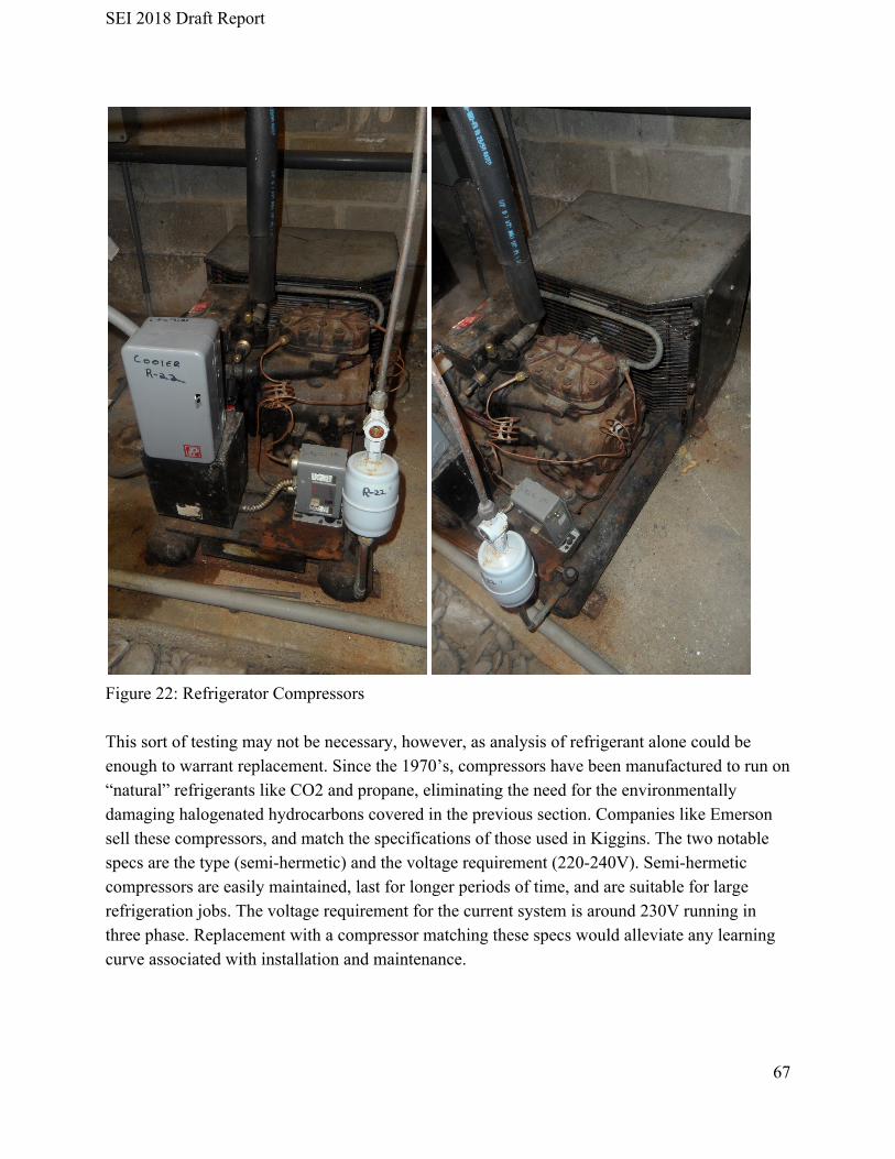
SEI 2018 Draft Report
Figure 22: Refrigerator Compressors This sort of testing may not be necessary, however, as analysis of refrigerant alone could be enough to warrant replacement. Since the 1970’s, compressors have been manufactured to run on “natural” refrigerants like CO2 and propane, eliminating the need for the environmentally damaging halogenated hydrocarbons covered in the previous section. Companies like Emerson sell these compressors, and match the specifications of those used in Kiggins. The two notable specs are the type (semi-hermetic) and the voltage requirement (220-240V). Semi-hermetic compressors are easily maintained, last for longer periods of time, and are suitable for large refrigeration jobs. The voltage requirement for the current system is around 230V running in three phase. Replacement with a compressor matching these specs would alleviate any learning curve associated with installation and maintenance.
67

SEI 2018 Draft Report
4.5.3.2 Insulation The insulation in the system is very old, and insulation degrades over the years. The interns wanted to calculate how much heat was escaping into the system. In order to do that the interns first found the layers that insulated the system. The insulation is a two part urethane foam, which surrounds the system. On the top side, there is insulation, a plastic layer, and a piece of plywood. The left and right sides have insulation and a concrete masonry unit (CMU). The back is just a large CMU. The front side is a metal door, and CMUs.
Figure 23: A Layout of the Top Wall Figure 24: A Layout of the Back Wall
Figure 25: A Layout of the Side Walls
68

SEI 2018 Draft Report
The interns wanted to see how the temperature of the walls differed from the walls not touching the fridge system, so how much colder they were. An infrared temperature was utilized. Table 42: Temperature of the Outside Walls
The inside walls were also measured. Table 43: Inside Temperature of Fridge and Freezer Walls
The fridge and freezer on the walls represent the distinction between where the fridge ends and the freezer starts. Tom Johnson lended interns a thermal imaging device to show the temperature gradient on the outside wall of the fridge and freezer. Dark purple represents lower temperature heat seepage from the freezer.
69

SEI 2018 Draft Report
Figure 26: Infrared Picture of Left Outside Wall of System As for insulation, efficiency decreases with time as a result of waterlogging and material degradation. According to the U.S Army Corps of Engineers Cold Regions Research and Engineering Laboratory, after 5 years the R-value of urethane spray goes down by 55%. It has been much longer than 5 years since this insulation has been installed, so the insulation has gone down by more than 55%, but the exact number is unknown. The utilized thickness of insulation has also increased over the years. The company, U.S Cooler, requires that for the walls and ceiling of the freezer coated in polyurethane be at least 4 inches thick. 4.5.3.3 Defroster and Evaporator The defroster is used to defrost the system’s coils when frost builds up on them. When they get too covered, the system has to work harder, which decreases the efficiency and increases the energy usage. The defroster should also only come on when needed, as to not waste energy. Ross Hansen introduced the interns to the company KE2Therm, which has already been implemented in some of Cornell’s refrigeration systems, saving the university thousands of dollars in energy cost. KE2Therm was contacted, and a webinar information session was set up. The KE2 Evaporator Efficiency was determined to be the best option for SML. It is a “smart” system that controllers heating, temperature, fan cycles, compressor runtime, and demand defrosts. It can be installed on the fridge wall, the evaporator fans, or outside the fridge door. Although placing it on the fridge door is not the best place for a commercial kitchen.
70

SEI 2018 Draft Report
Figure 27: KE2Therm Evaporator Efficiency Device KE2Therm only supplies devices to make the system more efficient; however, Shoals may needs to also replace the compressors. KE2Therm relayed a company, Refrigeration Trenton Products. They sell condensers, evaporators, and coils. 4.5.4 System Replacement Since the system is so old, instead of replacing aspects of the current system, the entire system can be replaced. The original manufacturer, Crown-Tonka, still produces walk-in systems. The systems are built to fit the space and specifications, so the format of the freezer behind the fridge can be reestablished. The insulation, non-HCFC ENVIROFOAM™, is urethane spray foam. The spraying of the insulation has zero ozone depletion potential since it is made of soybean oil and plastic water bottles, so it is environmentally friendly. The thickness of the insulation can be between between 3.5 in and 6 in, which is already much thicker than the current make. The system also comes with LED lights, which is a problem in the current system. This new modern system also has an Electronically Commutated “EC” evaporator motor. According to InterLink, a Commercial Refrigeration Parts Company, EC motors are more efficient than other evaporator motors, Shaded Pole and permanent split-capacitor (PSC) motors. And Crown Tonka claims EC evaporator motors are 60% more efficient than shaded pole motors and 40% more efficient than PSC motors. Crown-Tonka also offers a “smart” control refrigeration system. Similar to the KE2Therm Efficiency Evaporator, the defroster will only be utilized when needed.
71
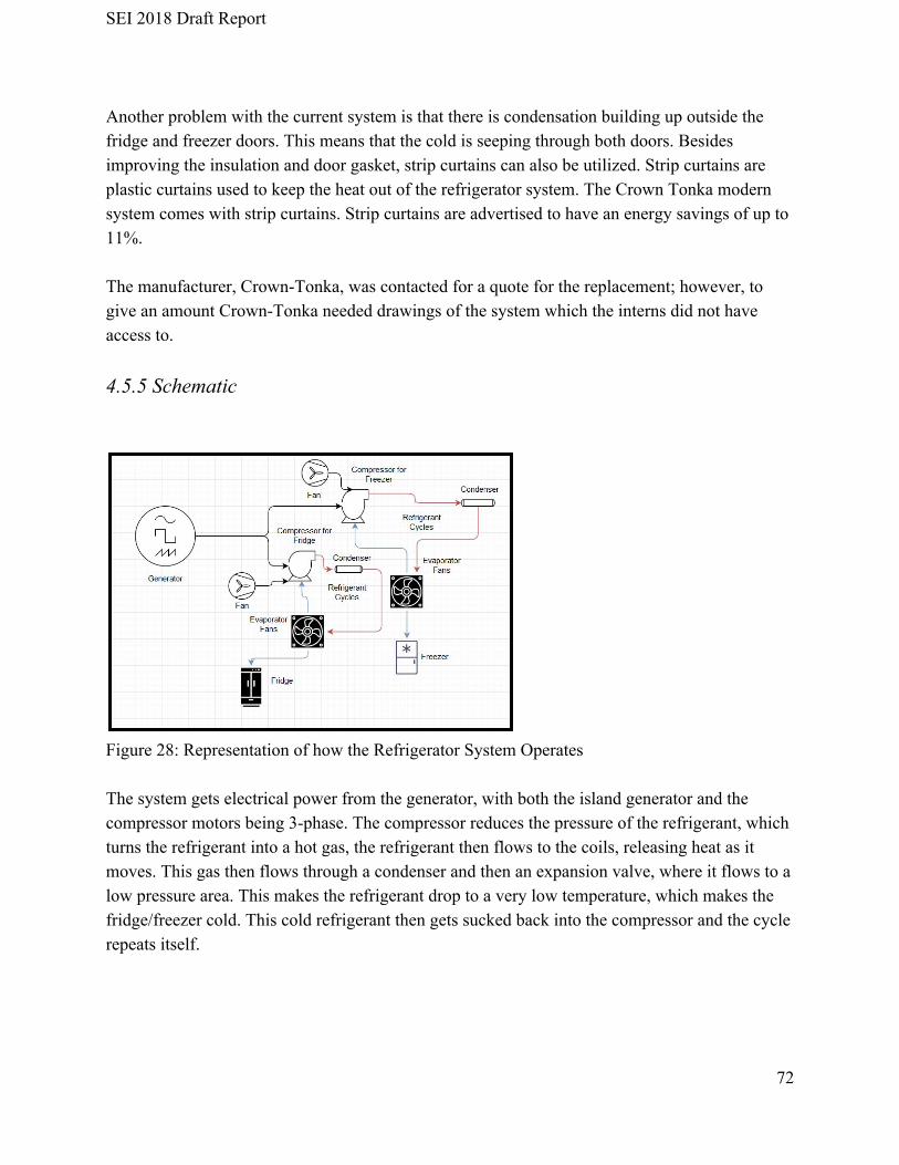
SEI 2018 Draft Report
Another problem with the current system is that there is condensation building up outside the fridge and freezer doors. This means that the cold is seeping through both doors. Besides improving the insulation and door gasket, strip curtains can also be utilized. Strip curtains are plastic curtains used to keep the heat out of the refrigerator system. The Crown Tonka modern system comes with strip curtains. Strip curtains are advertised to have an energy savings of up to 11%. The manufacturer, Crown-Tonka, was contacted for a quote for the replacement; however, to give an amount Crown-Tonka needed drawings of the system which the interns did not have access to. 4.5.5 Schematic
Figure 28: Representation of how the Refrigerator System Operates The system gets electrical power from the generator, with both the island generator and the compressor motors being 3-phase. The compressor reduces the pressure of the refrigerant, which turns the refrigerant into a hot gas, the refrigerant then flows to the coils, releasing heat as it moves. This gas then flows through a condenser and then an expansion valve, where it flows to a low pressure area. This makes the refrigerant drop to a very low temperature, which makes the fridge/freezer cold. This cold refrigerant then gets sucked back into the compressor and the cycle repeats itself.
72

SEI 2018 Draft Report
4.6 Conclusions and Recommendations Since the system is so old, most of the components should be replaced. The insulation is not only thinner than modern insulations, but has also accumulated water content over the years which decreases its ability to prevent heat flow. The compressor and refrigerants should also be updated with more modern and environmentally friendly options. If the entire system is not replaced, then there are updates that can be implemented on the current system. Automatic LEDs should replace the incandescents. Door gaskets must be replaced and strip curtains could be installed to prevent cool air from escaping when the door is opened. Since R-22 is encountering strict legislation, the refrigerant should be replaced with CO2 or propane. In order to do this, SML should consider look into replacing the compressor; a couple of favorable options are offered by Emerson. A variable frequency device should also be implemented to improve the energy efficiency of the compressor motors. KE2Therm’s efficiency evaporator should also be installed to further control the mechanisms of the system. It is recommended that SML replace things like the gaskets and refrigerator fans in the short term. Since more information is needed to make a decision on the compressor replacement or complete reconstruction, SML should contact the various manufacturers to get a better idea about price and installation. 4.7 References Justin Ulrich, Unitil Ross Hansen, SML “Specifications.” Cooler Connection Blog, www.uscooler.com/specifications/. “Truth About Insulation.” Truth About Insulation | American Walk in Coolers, www.americanwalkincoolers.com/insulation.html. Bohne, Russell. About Us | EnviroFoamInsulation.com, www.envirofoaminsulation.com/index.php/about-us “Walk In Cooler & Freezer.” Everidge, www.everidge.com/products/walk-ins/.
73

SEI 2018 Draft Report
“How Does a Refrigerator Work?” Real Simple, Real Simple, www.realsimple.com/food-recipes/tools-products/appliances/how-does-refrigerator-work. Center for Food Safety and Applied Nutrition. “Consumers - Refrigerator Thermometers: Cold Facts about Food Safety.” U S Food and Drug Administration Home Page, Center for Biologics Evaluation and Research, www.fda.gov/Food/ResourcesForYou/Consumers/ucm253954.htm. Xiang, B., Patra, P., Montzka, S., Miller, S., Elkins, J., Moore, F., Atlas, E., Miller, B., Weiss, R., Prinn, R. and Wofsy, S. (2014). Global emissions of refrigerants HCFC-22 and HFC-134a: Unforeseen seasonal contributions. Chemours.com. (2018). Freon™ 408A (R-408A) refrigerant. [online] Available at: https://www.chemours.com/Refrigerants/en_US/products/Suva/Suva408A.html [Accessed 12 Jul. 2018]. Linde-gas.com. (2018). Refrigerants Environmental Data. [online] Available at: http://www.linde-gas.com/en/images/Refrigerants%20environmental%20GWPs_tcm17-111483.pdf [Accessed 12 Jul. 2018]. Spletzer, S. (2010). Choosing the Right R-22 Retrofit. [online] Epa.gov. Available at: https://www.epa.gov/sites/production/files/documents/Choosing_Right_R22_Retrofit.pdf [Accessed 13 Jul. 2018].
74

SEI 2018 Draft Report
Assignment 5: Wastewater - Solids Solutions Project Leads: Takeru Nishi and Jake Shactman 5.1 Background Appledore’s wastewater is collected in three main septic tanks where liquids are separated from solids and are fed into one of two leach fields. A majority of the wastewater flow is downhill from the dorms to leach field one, a plot of land adjacent to Kiggins commons. Since gravity drives the movement of waste from the dorms, there is no need for a pumping system. However, the location of the north septic tanks requires that there be a pumping station to transport waste uphill to the main leach field. Though the leach fields are effective for disposal of liquid effluent, accumulation of sludge presents an issue. Once the solids within the septic tanks reach a certain height, typically after 3-4 years, they must be removed through a costly process of transporting sewage trucks from the mainland; this venture can cost upwards of $20,000. Recently, island coordinators came into contact with SludgeHammer, a company that markets a product that has potential to sustainably decompose solid waste. SludgeHammer’s system relies on the pumping of the outside air into the septic tanks to activate a proprietary blend of bacteria. Once activated, the decomposition of sludge within the tank shifts from anaerobic to aerobic digestion, the former being a contributor to the thick sludge layer accumulating in the tank. Prior to the installation, interns met with the New England distributor of SludgeHammer products, Gregory Teren. This meeting provided the interns with a better idea of how the system operates. A basic schematic of the system is shown in figure 30, taken from the SludgeHammer website.
Figure 30: Schematic of the SludgeHammer System
75

SEI 2018 Draft Report
Of the many impressive claims made by the SludgeHammer, the most intriguing is that the decomposition of waste material by the bacteria is so complete that the need to pump the tanks is virtually eliminated. If this system is to work as planned, SML would be alleviated of its wastewater concerns. However, with the SludgeHammer installed in an unfamiliar environment under non ideal conditions (i.e. tanks were not pumped 6-8 months in advance and the system will be turned off in the winter), these claims will be tested. 5.2 Purpose The purpose of this project is to evaluate the effectiveness of the SludgeHammer product and determine if this would be a viable solution to eliminate or reduce the need for sludge pumpouts. With the purchase of one SludgeHammer S-46 unit, the interns were able to gather data and monitor the system post installation to determine the effectiveness of the product. 5.3 Scope The interns researched and evaluated the SludgeHammer wastewater system to determine whether this would be a viable solution to reduce sludge buildup. 5.4 Methods 5.4.2 Sludge Judge In order to determine the total amount of sludge within the tanks prior to installation of the SludgeHammer, a Sludge Judge was used to measure the depth of settled solids within each septic tank throughout the island. Each of the 7 tanks on the island were tested, including the 3 lower tanks, 2 tanks by Kiggins (location of Sludge Hammer installation), and 2 tanks behind Bartells Hall. To use the Sludge Judge, the device is slowly lowered to the bottom of the tank. The float valve allows materials into the tube on the way down but acts as a stopper once the device is lifted up from the tank. From here, a depth of settled solids can be taken using a measuring tape. To estimate the volume of settled solids, this depth found is multiplied by the cross sectional area of the tanks. 5.4.1 Data Collection With the assistance of wastewater expert Dr. Nancy Kinner and SML’s Director of Operations Mike Rosen, it was determined that BOD, TSS, DO, & pH would be the most effective means of determining whether the SludgeHammer is working as promised. Due to the limited amount of
76

SEI 2018 Draft Report
time interns have on the island and the lack of necessary laboratory materials, biological oxygen demand (BOD) and total suspended solids (TSS) were outsourced to the UNH Water Quality Analysis Laboratory for testing. Both pH and dissolved oxygen (DO) could be determined using YSI probes provided by SML. Following the installation of the SludgeHammer on June 27, multiple samples were taken for the purpose of testing BOD, TSS, and pH levels in the septic tanks. Six 250mL amber polyurethane test bottles were filled with the fluid in the first Kiggins septic tank. Three of these bottles were labed TSS and the other three BOD. Samples were taken around 4 hours after turning the mixer on to allow for the settled sludge and floating scum layer to create a homogenous slurry. Instructions for the handling of samples were provided by the UNH Water Analysis Lab, the two most important are as follows: keep the samples around 40˚F and testing must be done within 48 hours to avoid degradation of the contents. Samples were then shipped to Portsmouth a day later on June 27th at 3pm, where they were picked up by Ross Hansen and brought to the lab. 5.5 Results and Analysis 5.5.1 Settled Solids - “Sludge” Representatives from SludgeHammer made it clear that the system would create significant improvements to the septic tank even over a short time period of a couple weeks. Using the Sludge Judge, interns were able to collect baseline data of the amount of sludge in each tank prior to installation of the SludgeHammer. Also, the cross sectional area of the septic tanks was measured to be 120” x 71” (8520 in2 = 59.17 ft2) assuming a 3” thickness of concrete. This data is shown below. Table 44: Amount of Solids Before SludgeHammer Installation
Tank Lower 1 Lower 2 Lower 3 Kiggins 1
Kiggins 2
Bartells 1 Bartells 2
Depth of Settled Solids Sludge (in)
12” 13” 5” 7” 3” 6” 2”
Volume of Solids (gal)
443 480 184 259 111 221 74
Comments Right (Middle scum layer too thick)
Middle Thick grease layer
Middle Middle Middle Middle Thick scum layer
Middle
77

SEI 2018 Draft Report
SludgeHammer recommends that the tank should be pumped 6 months prior to installation. Because of the excessive costs associated with pumping the septic tanks due to being located on an island, it was decided to use the tank with the least amount of solids. It was decided to use the Kiggins tanks as these had the least amount of sludge buildup at the time. However, this decision was made before the dorms reached peak occupancy. Interns gathered baseline data of each existing tank and found that the Bartels tanks actually had slightly less sludge buildup, contrary to previous testing. The depth of solids were monitored in the following weeks to analyze how the SludgeHammer affected the initial sludge depths throughout the tanks. As can be seen in Figures X and Y below, the sludge depths in tank one were minimal. A reduction in 2-3” was seen initially in tank 1, however, this was due to the solids being mixed into a more homogenous slurry. These solids included both the scum on top, which was broken up only a couple days after installation (excluding the scum before the first baffle near the inlet streams), as well as the sludge on the bottom which became agitated due to the aeration. After the initial agitation of tank 1, these suspended solids began to settle again as can be seen in the plateauing depth of solids. Another major factor which influenced this data was the release of the plastic filter in tank 1. Due to the heavy agitation in tank 1 due to mixing and aeration, the heavily turbid slurry clogged the filter between the two tanks. It was recommended by Dr. Wickham and Dr. Kinner to remove the filter entirely to allow flow to the second tank. This removal caused a rapid flow of heavily turbid wastewater to move into tank 2. This equilibration that occured brought a large amount of suspended solids into tank 2, which then settled and caused an increase in sludge depth. Sludge depths in tank 2 increased significantly from 2”-3” before installation to upwards of 10”.
78
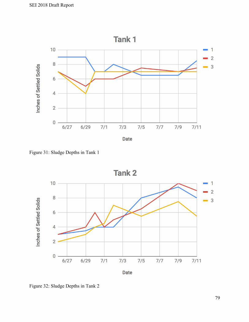
SEI 2018 Draft Report
Figure 31: Sludge Depths in Tank 1
Figure 32: Sludge Depths in Tank 2
79
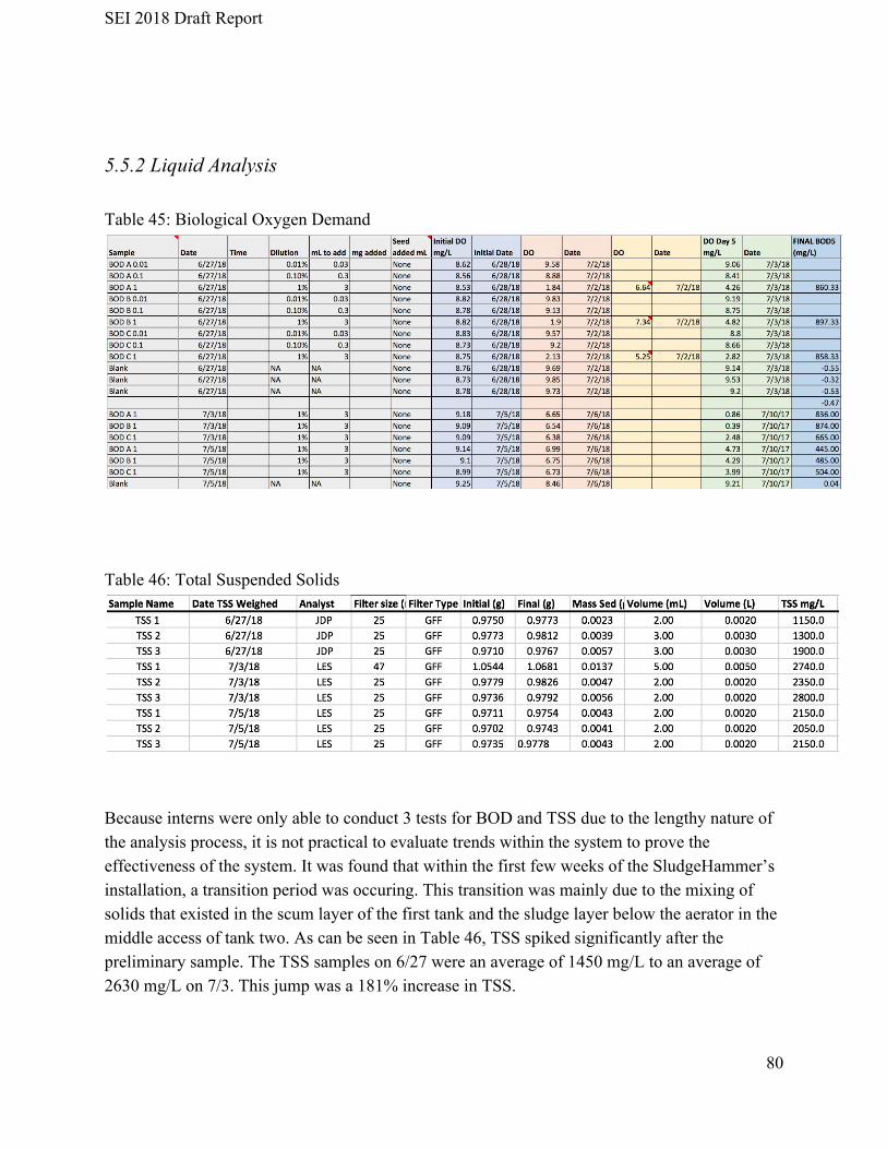
SEI 2018 Draft Report
5.5.2 Liquid Analysis Table 45: Biological Oxygen Demand
Table 46: Total Suspended Solids
Because interns were only able to conduct 3 tests for BOD and TSS due to the lengthy nature of the analysis process, it is not practical to evaluate trends within the system to prove the effectiveness of the system. It was found that within the first few weeks of the SludgeHammer’s installation, a transition period was occuring. This transition was mainly due to the mixing of solids that existed in the scum layer of the first tank and the sludge layer below the aerator in the middle access of tank two. As can be seen in Table 46, TSS spiked significantly after the preliminary sample. The TSS samples on 6/27 were an average of 1450 mg/L to an average of 2630 mg/L on 7/3. This jump was a 181% increase in TSS.
80

SEI 2018 Draft Report
Because of this significant increase in suspended solids within the first tank, the influent entering tank 2 saw an increase in sludge as these suspended solids were given time to settle after entering the second tank. During this same period from 6/27 - 7/3, sludge depths doubled from an average of 3” to 6”, respectively. Because there is a settling time necessary for the solids to enter the sludge layer, the sludge depth reaction was delayed and didn’t peak until 7/9 where sludge depths reached up to 10”. Because the TSS levels dropped 20% between 7/3 and 7/5 and the sludge depth levels also began dropping after peaking 7/9, the tanks may be starting to come back to an equilibrium as shown in the plateau within Figure 32. 5.5.3 Consultation with SludgeHammer CEO Dr. Dan Wickham On June 29, interns had a conference call with the CEO and inventor of SludgeHammer Dr. Dan Wickham, SludgeHammer’s New England Distributor Gregory Teren, wastewater treatment expert Dr. Nancy Kinner, and SML’s Director of Operations Mike Rosen. Both Dr. Nancy Kinner and Mike Rosen were both very skeptical of the system prior to installation. In efforts to debunk this skepticism, Dr. Wickham provided many facts of his experience with the system and how it was designed to function properly. First, Dr. Wickham stated that several systems dating back to 2000 have never needed to be pumped after installation. Of course, this depends on many factors such as the load on the system, which dictates the hydraulic retention time within the tanks. He also noted that single tank systems are not as effective. For SML, this is not a worry as all the systems have at least 2 tank systems. 5.5.4 Hydraulic Retention Time Dr. Dan Wickham suggested a hydraulic retention time (HRT) of 3 days. Hitting this 3 day HRT is essential as it allows the bacteria microbes enough time to break down the wastewater before being discharged into the leach field.
RT Q 67 gal/dayH = QV ⇒ = V
HRT = 3 days1110 gal = 3
In order to assure the HRT of at least 3 days, the flow would have to be greater than, or equal to 367 gallons/day. Using the flush logs deployed in each dorm, along with an inline water meter to measure the sink water used per dorm, the total flow for all three dorms is estimated to be 52 gallons/day through flushing and from using the sink.
RT 1 daysH = QV = 1110 gal
52 gal/day = 2
81

SEI 2018 Draft Report
5.6 Conclusions and Recommendations One of the main limitations with the study of the SludgeHammer was the time. Because the system was not installed until 6/27, interns were only able to get 3 samples of TSS/BOD tested. Another factor that limited the amount of data collected was that the BOD test requires a 5 day incubation period. It is recommended that the island continues to monitor the Kiggins septic tanks. At the very least, sludge thickness should be monitored to determine if any of the settled solids are being processed by the bacteria added by SludgeHammer. More bacteria was added by Mr. Teren on 7/11 to combat the increase in sludge depth in tank 2. The circulation pump was also turned off in tank 2 to allow for solids to settle before entering the leach field. Because of the significant increase in solids in tank 2, Mr. Teren suggested adding a second tank bottom diffuser to increase aeration and encourage bacterial digestion. If this is decided upon, it will be essential for the turbidity within the distribution box to be closely monitored. As seen in the initial installation, the mixing caused by aeration creates in increase in turbidity within the tank and can cause clogging and solid overflow. Because aeration is being proposed in the second tank, it will be essential to ensure solids are not entering the leach field as this would create a problem in itself. Overall, no conclusion can be made in terms of the effectiveness of the system. Using the baseline data gathered this year, it will be useful to monitor the the tanks sludge depths in the future to determine if there is any long term success. 5.7 References Gregory Teren & Dr. Dan Wickham - SludgeHammer Dr. Nancy Kinner
82

SEI 2018 Draft Report
Assignment 6: Rooftop Water for Flushing Toilets in Dorm 1, 2 and 3 Project Leads: Jake Shactman and Laurel He 6.1 Background SML relies on a 20-foot dug well for the majority of its potable water with supplemental water production using reverse osmosis as required. A portion of this potable water is currently being used to flush toilets. In 2017, SML revived an old cistern for rainwater collection and installed a pump and pressure tank system for distribution at Bartels Hall for flushing toilets. The two tanks at Bartels Hall currently hold 4,443 gallons of water and are each 9’x6’x5’6” and are likely left over from the lifesaving station that previously existed on Appledore Island. These tanks were evaluated in 2009 by SEI’s and were determined to be adequate for the demand created by Bartel’s Hall. However, since 2009, factors such as the movement towards low flush toilets have cut the water demand 68% from flushing. With the implementation of low flush toilets throughout the Island, SML has reduced the water demand per flush from 5 gallons to 1.6 gallons. 6.2 Purpose The purpose of this project is to evaluate the several design factors that dictate the sizing of the water tank, or cistern. These factors include the demand created by the toilets in dorm 1, 2, and 3, average rainfall, and the size of the roof. It is essential to evaluate each of these factors to ensure the tanks are sufficient to supply the dorms through the dryer periods of the summer. 6.3 Scope The interns evaluated dorms 1, 2, and 3 as a potential source of rainwater collection to reduce the fresh water demand on the well. Several alternatives were proposed and analyzed to determine the optimum design. It was found that the implementation of a rainwater collection system could save SML 4,400 gallons each season in freshwater. 6.4 Methods 6.4.1 Water Demand To determine the total demand of water for each dorm bathroom, flush data was gathered for Dorm 1, Dorm 2, Dorm 3, and Bartels Hall. This data was gathered by implementing tally sheets
83

SEI 2018 Draft Report
for each day of the week where users placed a tally for each flush From the total amount of flushes, the amount of flow can be found:
Flow (gal) = # of flushes * 1.6 gallons of water/flush. Eqn. 7 The total number of flushes was divided by the occupancy of each dorm to get an average flush count per person. This average was then multiplied by 20 to ensure the design was taking into account full occupancy. 6.4.2 Rooftop Analysis In efforts to get an idea of how much water can be gathered for a given rainfall amount, interns worked with Dr. John Durant of Tufts University to measure the rooftops of dorms 1, 2, and 3. To do so, using measuring tapes, the length and widths were measured for each building. 6.4.3 Rainfall Data Using average monthly rainfall data collected from May 2000 - June 2018 from Portsmouth, NH, interns were able to build off the rooftop analysis to predict seasonal water retention (gallons) based off of average, high, and low precipitation months. To account for the variability in potential future rainfall, high and low precipitation events were also evaluated. This helps determine whether the cisterns are able to hold enough water even during drier months. The theoretical volume of water retained was determined by multiplying the area of rooftop by the depth of rainfall. This was evaluated on a monthly basis. 6.4.4 Retention Rate Building off of the 2017 study, the interns last year were not able to determine the percentage of water that actually gets into the cistern because they did not have access to accurate rainfall data for Appledore. With the installation of the rainfall gauge Spring 2018, interns were able to calculate the rise in water level in respects to a rain event. To determine what the percentage of water that falls on the roof in respect to the total amount of water that ends up in the cistern, interns evaluated the existing rooftop rainfall collection system at Bartells Hall. Interns found the area of the roof above the gutters and gathered data from a rainfall gauge next to the Energy Conservation Building. The cistern level of Bartels was measured over a 24 hour period using a Solinst Water Meter, and the was found. UsingDepthΔ this data, and the avg # of flushes/day, a retention rate can be found. This value represents the amount of water that accumulates in the cistern to the amount of rainwater that theoretically
84

SEI 2018 Draft Report
lands on the rooftop. This will then be taken into account when designing the cistern size for the proposed rainwater collection system for dorms 1, 2, and 3. The retention rate can be calculated as:
etention %R = ΔDepth (f t) (Area of Cistern (f t )) 7.48 gal/f t*2
*3
[Rainfall (f t) (Area of Roof (f t ) (7.48 gal/f t )] −[(# of f lushes over the duration of the storm) 1.6 gal/f lush]* 2 * 3 *
6.5 Results and Analysis 6.5.1 Flush Data Before any alternatives solutions can be assessed to eliminate the need to use well water for flushing in dorms 1, 2, and 3, the total current demand needs to be determined for each of these buildings. Using flush counts from over a week’s sample size, this demand can be seen in Table 47 below. An average of 500 gallons per dorm was determined to be the demand that will be designed for. Table 47: Flush Count (2018)
Flush Count June 25th 26th 27th 28th 29th 30th 1st Total
Dorm 1 8 5 7 10 8 6 7 51
Dorm 2 4 4 7 5 3 7 5 35
Dorm 3 4 7 9 8 11 8 15 62
Bartels 7 6 3 6 13 8 9 52
Table 48: Water Usage per Person (2018)
Water Usage (gal/person)
June 25th 26th 27th 28th 29th 30th 1st
Avg gal / person*week
Gal / Week (Assuming full dorm occupancy)
Gal / Month (Assuming full occupancy)
Dorm 1 0.71 0.44 0.70 1.00 0.80 0.60 0.70 4.96 99.11 396.44
Dorm 2 0.71 0.71 1.24 0.73 0.44 1.24 0.80 5.87 117.49 469.98
Dorm 3 0.91 1.40 0.90 0.80 1.10 0.80 1.41 7.33 146.52 586.08
Bartels 1.40 1.20 0.53 1.07 2.31 1.28 1.44 9.23 138.47 553.87
85

SEI 2018 Draft Report
6.5.2 Retention Rate Interns found the area of the roof above the gutters to be about 800 ft2. To get precise rainfall data, interns were able to gather data from a rainfall gauge that was installed next to the Energy Conservation Building in Spring 2018. Using this gauge, it was found that 0.39” of rain fell over the 24 hour period from 8pm on 6/27 through 8pm on 6/28. The cistern level of Bartels was measured at 8pm on 6/27 and again at 8pm on 6/28 which resulted in a of 0.46 ft. UsingDepthΔ this data, and the # of flushes over that 24 hour period, a retention rate was found. This value of 94.1%, represents the amount of water that accumulates in the cistern to the amount of rainwater that theoretically lands on the rooftop. This will then be taken into account when designing the cistern size for the proposed rainwater collection system for dorms 1, 2, and 3.
etention %R = ΔDepth (f t) (Area of Cistern (f t )) 7.48 gal/f t*2
*3
[Rainfall (f t) (Area of Roof (f t ) (7.48 gal/f t )] −[(# of f lushes over the duration of the storm) 1.6 gal/f lush]* 2 * 3 *
4.1% = 0.46 f t 51 f t 7.48 gal/f t*
2*
3
[0.39 in (1 f t/12 in) (800 f t ) (7.48 gal/f t )] − [(5 f lushes) 1.6 gal/f lush]* * 2 * 3 *= 186.5
175.5 = 9
6.5.3 Alternative/Cost Analysis The goal of this study is to determine a system to supply dorms 1, 2, and 3 with grey water for toilet flushing. Many aspects go into determining the best system. These aspects are based off of the amount of water supply and water demand, which take into account the area of the roof, historical rainfall data, occupancy of the dorms, flushing behavior of occupants. Along with this, the system must also be the most cost and energy efficient option. To determine the optimum alternative, three gutter/cistern schemes were evaluated:
➔ Alternative 1: One large cistern to supply 3 dorms This alternative would be the most cost efficient as only one pump, one cistern, and one pressure tank would be required.
Table 49: Gutters around 1 dorm building - 1 cistern/pumping system to supply 3 dorms
Average Month
Avg Rainfall (in)
Volume of Water Accumulated (1 Dorm) (gal)
Demand/ Dorm Total Demand
Theoretical left over water (end of month)
Left over water assuming 90% retention
May 4.07 4795 500 1500 3295 2815
June 4.33 5101 500 1500 6896 5906
July 3.97 4677 500 1500 10073 8616
August 3.34 3935 500 1500 12508 10657
Total 15.71 18508 2000 6000 12508 10657
86

SEI 2018 Draft Report
Best Case* Month
High Rainfall (in)
Volume of Water Accumulated (1 Dorm) (gal)
Demand/ Dorm Total Demand
Theoretical left over water
Left over water assuming 90% retention
1.15*Avg May 4.68 5514 500 1500 4014 3463
June 4.98 5866 500 1500 8380 7242
July 4.57 5379 500 1500 12259 10583
August 3.84 4525 500 1500 15284 13156
Total 18.07 21284 2000 6000 15284 13156
Worst Case* Month
Low Rainfall (in)
Volume of Water Accumulated (1 Dorm) (gal)
Demand/Dorm Total Demand
Theoretical left over water
Left over water assuming 90% retention
0.85*Avg May 3.46 4076 500 1500 2576 2168
June 3.68 4336 500 1500 5412 4570
July 3.37 3975 500 1500 7887 6648
August 2.84 3345 500 1500 9732 8159
Total 13.35 15732 2000 6000 1283 8159
➔ Alternative 2: One cistern for dorms 1 and 2 and another for dorm 3
Because dorms 2 and 3 are only 62’ from each other, this alternative would be more feasible but still more costly than alternative 1.
Table 50: Gutters around 1 Building Supplying Dorms 2 & 3
Average Month
Avg Rainfall (in)
Volume of Water Accumulated (1 Dorm) (gal)
Demand - Dorms 2 & 3
Theoretical left over water
Left over water assuming 90% retention
May 4.07 4795 1000 3795 3315
June 4.33 5101 1000 7896 6906
July 3.97 4677 1000 11573 10116
August 3.34 3935 1000 14508 12657
Total 15.71 18508 4000 14508 12657
Best Case* Month High Volume of Water Demand - Theoretical Left over water
87

SEI 2018 Draft Report
Rainfall (in)
Accumulated (1 Dorm) (gal)
Dorms 2 & 3 left over water
assuming 90% retention
1.15*Avg May 4.68 5514 1000 4514 3963
June 4.98 5866 1000 9380 8242
July 4.57 5379 1000 13759 12083
August 3.84 4525 1000 17284 15156
Total 18.07 21284 4000 17284 15156
Worst Case* Month
Low Rainfall (in)
Volume of Water Accumulated (1 Dorm) (gal)
Demand - Dorms 2 & 3
Theoretical left over water
Left over water assuming 90% retention
0.85*Avg May 3.46 4076 1000 3076 2668
June 3.68 4336 1000 6412 5570
July 3.37 3975 1000 9387 8148
August 2.84 3345 1000 11732 10159
Total 13.35 15732 4000 11732 10159
➔ Alternative 3: One cistern for each dorm
This alternative has the most up front cost as three pumps, three cisterns, and three pressure tanks would be needed.
Table 51: Gutters around half of one dorm - 3 cisterns to supply each dorm respectively
Average Month
Avg Rainfall (in)
Volume of Water Accumulated / 1/2 Dorm (gal)
Demand/ Dorm
Theoretical left over water
Left over water assuming 90% retention
May 4.07 2397 500 1897 1658
June 4.33 2551 500 3948 3453
July 3.97 2339 500 5787 5058
August 3.34 1967 500 7254 6329
Total 15.71 9254 2000 7254 6329
Best Case* Month
High Rainfall (in)
Volume of Water Accumulated (gal)
Demand/ Dorm
Theoretical left over water
Left over water assuming 90% retention
1.15*Avg May 4.68 2757 500 2257 1981
June 4.98 2933 500 4690 4121
July 4.57 2689 500 6880 6042
88
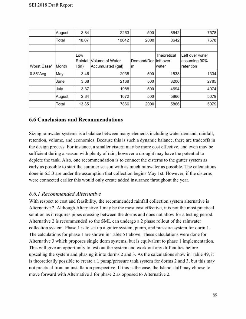
SEI 2018 Draft Report
August 3.84 2263 500 8642 7578
Total 18.07 10642 2000 8642 7578
Worst Case* Month
Low Rainfall (in)
Volume of Water Accumulated (gal)
Demand/Dorm
Theoretical left over water
Left over water assuming 90% retention
0.85*Avg May 3.46 2038 500 1538 1334
June 3.68 2168 500 3206 2785
July 3.37 1988 500 4694 4074
August 2.84 1672 500 5866 5079
Total 13.35 7866 2000 5866 5079
6.6 Conclusions and Recommendations Sizing rainwater systems is a balance between many elements including water demand, rainfall, retention, volume, and economics. Because this is such a dynamic balance, there are tradeoffs in the design process. For instance, a smaller cistern may be more cost effective, and even may be sufficient during a season with plenty of rain, however a drought may have the potential to deplete the tank. Also, one recommendation is to connect the cisterns to the gutter system as early as possible to start the summer season with as much rainwater as possible. The calculations done in 6.5.3 are under the assumption that collection begins May 1st. However, if the cisterns were connected earlier this would only create added insurance throughout the year. 6.6.1 Recommended Alternative With respect to cost and feasibility, the recommended rainfall collection system alternative is Alternative 2. Although Alternative 1 may be the most cost effective, it is not the most practical solution as it requires pipes crossing between the dorms and does not allow for a testing period. Alternative 2 is recommended so the SML can undergo a 2 phase rollout of the rainwater collection system. Phase 1 is to set up a gutter system, pump, and pressure system for dorm 1. The calculations for phase 1 are shown in Table 51 above. These calculations were done for Alternative 3 which proposes single dorm systems, but is equivalent to phase 1 implementation. This will give an opportunity to test out the system and work out any difficulties before upscaling the system and phasing it into dorms 2 and 3. As the calculations show in Table 49, it is theoretically possible to create a 1 pump/pressure tank system for dorms 2 and 3, but this may not practical from an installation perspective. If this is the case, the Island staff may choose to move forward with Alternative 3 for phase 2 as opposed to Alternative 2.
89

SEI 2018 Draft Report
As for the cistern size, a manuscript written by Penn State researchers recommend cisterns to be either 1/4 of the annual demand, or 3 months of supply. ¼ of the annual demand for dorm 1 would account for 500 gallons whereas a 3 month supply would account for 1500 gallons. Ideally, the bigger the tank the less likely it is to run out of freshwater. This would make the optimum size 1500 gallons (3 months supply). Because the Island is seasonal, and there is little time to accumulate water before demand begins, ¼ of the total demand would not be enough to ensure the dorm could get through a dry season without having to revert back to well water. It is recommended that the cisterns allow for at least 1000 gallons of storage per dorm. This equates to two months of total storage capacity per dorm. 6.6.2 Water Savings In conclusion, while monitoring the flush counts throughout the dorms and comparing the total gallons used for flushing (full occupancy) per week of 363.13 gallons to the total gallons of water used by the island of 8303.91 gallons for the week, the Island used 4.37% of its’ water that week just through flushing in the dorms. By implementing a rainwater collection system to eliminate the draw from the well for this purpose, an estimated 4,400 gallons can be saved throughout the peak 3 month period of mid May - mid August. That savings is equivalent of about 4 days of the total islands water usage. 6.6.2 Winterizing Because Appledore is located primarily on bedrock with little topsoil, it would be very difficult to bury a cistern without blasting. This means that the cistern will likely have to be above ground, and exposed to the freezing climate during the winter months. One of the main concerns is freezing of the pump and piping systems because this can potentially cause severe damage to both components will burst and the pump will be damaged. Because of this, it will be necessary to store this system indoors during winter months. It is also recommended to drain the tanks after each season to rid the tank of any solids that may settle in the bottom of the tanks. It is not recommended to allow for the tanks to be filled throughout the winter due to concerns in regards to the structural integrity of the plastic tanks. Because nobody is on the island and the grid is shut down in the winter, other novelty remedies such as mixing, aeration, or heating of the tanks to prevent freezing is not a feasible option. 6.7 References https://www.wunderground.com/weather/us/nh/portsmouth/03801 https://extension.psu.edu/rainwater-cisterns-design-construction-and-treatment http://www.plastic-mart.com/category/109/plastic-storage-tanks https://www.plasticwatertanks.com/p/bqkfn/1000-gallon-rainwater-harvesting-tank-pm1000rh?gclid=EAIaIQobChMI853C3aSc3AIVFI_ICh22bwlGEAQYBCABEgIhxvD_BwE
90

SEI 2018 Draft Report
Assignment 7: Appledore Transportation Analysis Project Leads: Jake Shactman and Takeru Nishi 7.1 Background The effective movement of materials is critical to the operation of SML. This includes movements to, around, and off the island. These materials include: food, luggage, fuel, and supplies. Over the years, SML has had different types of vehicles ranging from large trucks with gasoline engines to golf carts. One of the most prominent difficulties encountered on Appledore is the terrain. This complicates transportation of goods, as pathways must be constructed to avoid steep inclines and barriers, and must be large enough to allow the island’s various vehicles to use them. For this reason, finding a vehicle that can both be well equipped for the terrain and environment and reliably perform all the necessary transportation functions is a challenge. Along with terrain, the harsh marine environment also causes corrosion issues throughout the fleet of vehicles. As SML evolves, it will continue with the focus on sustainability, and an evaluation of it vehicles is necessary to reach this goal. Currently, all seven vehicles on the island are powered by diesel. While SML has significantly reduced its use of fossil fuels over the past few years via installation of solar and wind energy, transitioning its vehicles over electric power is not as simple. However, careful monitoring of vehicle use can give some insight into the effect these vehicles have on overall island sustainability initiatives. 7.2 Purpose The purpose of this project is to gain a better understanding of the existing inventory of vehicles by studying the amount and type of usage for each vehicle and trailer. The ultimate goal of this study is to make recommendations based on the current vehicle conditions, cost of alternatives, sustainability of alternatives, and ease of maintenance practicality. 7.3 Scope Since island transportation is used by staff for various usages, interns had to effectively communicate the importance of accurate data collection. Over the span of one week, all users were asked to record every use of the island vehicles. With the help of island staff, precise data
91

SEI 2018 Draft Report
was collected, allowing the interns to make a detailed analysis on transportation use. From this analysis, recommendations were made to improve the transportation systems throughout the Island. 7.4 Methods 7.4.1 Inventory The first task of the transportation analysis was to get a full inventory of each mode of transportation throughout the Island. The island holds several different types of vehicles to serve a variety of needs for staff, students, visitors, and interns. Trailers were also included within the inventory and overall analysis, as these are important pieces of equipment to move larger loads in, out, and around the island. To take a thorough inventory, interns recorded the vehicle type, make, model, year, number of miles, primary uses, typical routes, and place of storage. Interns also measured the dimensions of the beds of the vehicles to account for the size of load each could carry. This comprehensive inventory is necessary to further analyze the efficiency of each vehicle. 7.4.2 Usage To help monitor the means and methods of transportation use throughout the Island, interns created a usage log that was deployed from 6/25-7/2. Island staff were instructed to fill out a log that tracked what is being moved, where materials are being moved, and how they are being moved. In efforts to understand what vehicles draw the most fuel consumption, and what materials effect this the most, staff members were asked to record before and after readings of the hour meter or mileage odometer. Using the fuel efficiency rates of each piece of equipment, interns could evaluate the total consumption of fuel. 7.4.3 Tow Capacity of John Deere Tractor To test the capacity of the tractor, a heavy duty chain was used to attach the frame of the tractor to the front of the Ford F-350 pickup truck. Because we know the weight of the truck is approximately 7,000 pounds, an experiment was attempted to tow the truck using the tractor. This would help determine whether a new truck would be needed or if it could be replaced with a dump trailer. The test was conducted starting at the high tide dock and continuing up the hill.
92

SEI 2018 Draft Report
7.5 Results and Analysis 7.5.1 Inventory Table 52: Inventory Vehicle Type
Make/Model
# of Miles/Hours (6/20)
# of Miles/Hours (7/2)
Avg # Miles/Hours per day
Tractor John Deere 4300 - 300CX Loader
441 hours
445 hours 0.33 hours/day
Trailer 9’ x 5’ x 1.5’
Venture Single Axle
N/A N/A N/A
Backhoe Case 580m Series 2
1135 hours N/A N/A
Dump Truck 8’ x 6’11” x 1’7”
1996 Ford F350 Power Stroke Diesel
136,869.1 mi 136,870.8 mi 0.14 mi/day
Gator #1 John Deere Gator
92.0 hours 99.4 hours 0.62 hours/day
Gator #2 John Deere Gator
167.5 hours 172.6 hours 0.43 hours/day
Gator #3 John Deere Gator
1068.5 hours 1079.5 hours 0.92 hours/day
93

SEI 2018 Draft Report
7.5.2 Usage Trends Usage trends were divided into several categories based on what was moved using the vehicle. These include:
● Equipment/Gear/Supplies: Lab equipment, dive gear, tools, machinery, etc ● Goods/Personal Items: Food, luggage, miscellaneous personal items ● Waste Removal: Garbage or recycling removal ● People: Anytime a vehicle is used for personal transportation
John Deere 4300 + 300CX Loader:
Figure 33: Single axle trailer being pulled by the tractor
Figure 34: Tractor Usage
94

SEI 2018 Draft Report
Table 53: Tractor Usage
Tractor # of Uses Cumulative Hours Avg. Hours /
Use
Equipment/Gear/Supplies 4 0.70 0.18
Goods/Personal Items 3 1.20 0.40
Waste 0 0.00 N/A
People 0 0.00 N/A
Total 7 2 0.29
9’ x 5’ x 1.5’ Venture Single Axle Trailer: Table 54: Trailer Usage Trailer # of Uses
Equipment/Gear/Supplies 1
Goods/Personal Items 3
Waste 0
People 0
Total 4.00
Case 580m Series 2 Backhoe: Usage trends were not evaluated as this piece of equipment was deemed to be necessary and irreplaceable by SML operational staff. 1996 Ford F-350 Powerstroke Diesel Dump Truck:
Figure 35: Heavy rusting on the underbody
95

SEI 2018 Draft Report
Figure 36: Truck Usage Table 55: Truck usage Truck # of Uses Cumulative Miles Avg. Miles / Use
Equipment/Gear/Supplies 0 0.00 N/A
Goods/Personal Items 3 0.40 0.13
Waste 1 0.60 0.60
People 0 0.00 N/A
Total 4 1 0.25
As made apparent by the table, the dump truck is used quite sparingly, as it accumulated only a mile of use over a week’s span. It goes without saying that the truck’s use varies from week to week, as the need for large capacity vehicles is not consistent. However, the datum that is guaranteed week to week is the food transport from the docks to Kiggins commons. The volume and weight of food cannot be moved reliably with any other vehicle, leaving the dump truck as the only option. Another point of emphasis is the truck’s condition. Given that it is a 1996 model, wear and tear is expected, but the salty and humid air has accelerated deterioration, most noticeably in the iron frame. The underbody is almost completely rusted over, with chipping and cracking of paint and metal all around the outer edge of the bed. Though the system still functions acceptably, the structural stability must be questioned, as the ubiquitous oxidation is bound to weaken the metal.
96

SEI 2018 Draft Report
With all its issues, the dump truck is still a necessity because it performs tasks that the other vehicles cannot. In an effort to explore alternatives to the dump truck, the towing capacity of the tractor was measured by testing if it was capable of pulling the truck. If the tractor is able to tow the truck, rated at around 7000 pounds, a dump trailer could serve as a viable replacement. Testing was done on the steep hill connecting the north and south parts of the island; the dump truck was chained to the back of the tractor and pulled up the hill. Two trials were done: the first with an empty truck and the second with the truck full of groceries. The first trial was a success, but the second was not. Results from this test indicate that the tractor is capable of pulling a trailer large enough to cover all the necessary transport of goods, around 6000 lbs in total; dump trailers are discussed in the following section. John Deere Gators (3):
Figure 37: Gator Usage Table 56: Gator Usage
Gators # of Uses Cumulative Hours Avg. Hours /
Use
Equipment/Gear/Supplies 36 7.85 0.22
Goods/Personal Items 25 3.81 0.15
Waste 3 0.75 0.25
People 29 1.70 0.06
Total 93 14 0.15
97

SEI 2018 Draft Report
7.6 Conclusions and Recommendations 7.6.1 Gator Alternatives After a week of testing, it was clear that the 3 John Deere Gators were the most used vehicles throughout the island. The reasons for their popularity is two fold. First, its smaller size allows it to easily navigate the island’s tough terrain. Second, it can handle the transport of most equipment and goods. However, their constant use results in a significant usage of diesel, which is both costly to transport and involves the burning of fossil fuel, thus increasing SML’s carbon footprint. One alternative which solves the problem of fuel burning while maintaining the island’s need for a utility vehicle is an electric utility vehicle. With all 3 Gators accounting for 14 hours throughout just 1 week, that averages to almost 5 hours of run time per gator. Throughout SML’s operating period from mid May - mid September, this equates to 80 hours of run time per year per gator. To estimate the amount of gallons per hour these vehicles burn, we will use:
(Eqn. 8)P H (specif ic fuel consumption HP ) / F uel Specif ic W eight G = ×
P H (0.40 18.2) / 7.2 .011 gph gph G = × = 1 ≈ 1 Where the specific fuel consumption is 0.40 per HP and the fuel specific weight is 7.2 lb/gal. Given this estimate of 1 gallon per hour run time for each gator, it can be estimated that each Gator consumes 80 gallons per year, equating to 240 gallons for all 3 Gators. In terms of carbon emissions, approximately 5,376 pounds of CO2 is emitted each year from just Gator usage. In efforts to reduce SML’s carbon footprint, while also save money on purchasing and transporting fuel to Appledore, an electric utility vehicle of similar capacity could be a viable alternative. To thoroughly evaluate this alternative, a decision matrix can be seen below in Table 57. Assuming 3 Gators are necessary for island operation, design solutions will be assessed in the scenario as if one of the Gators needed to be replaced. Also, the criteria weight was determined via input from Ross and Mike. Each of the criteria were rated on a one to five scale of importance, five being the most crucial. Their ratings were then averaged to give the scaling factor used to calculate the final score in the right hand column.
98

SEI 2018 Draft Report
Table 57: Utility Vehicle Design Matrix
Design Criteria
Design Solutions
Fuel Type Engine/ HP
Power Distribution
Bed Box Dimension
Towing Capacity
Ground Clearance
Base Price
Total Score
Criteria Weight
2.5 1 4 4.5 3.5 1.5 1
John Deere 6x4 Diesel Gator
Diesel 1*2.5=2.5
4cyl 18.2hp 1*1=1
4WD (6 Wheels) 5*4=20
45” x 52” x 12” 16.4 ft3
5*4.5=22.5
1,400 lb 4*3.5=14
6.4” 1*1.5=1.5
$12,849 1*1=1
62.5
John Deere 4x2 Electric Gator
Electric 5*2.5=12.5
48V DC 2*1=3
2WD 1*4=4
45” x 52” x 12” 16.4 ft3
5*4.5=22.5
500 lb 1*3.5=3.5
7.3” 2*1.5=3
$11,659 2.5*1=2.5
51
Polaris Ranger EV
Electric 5*2.5=12.5
30hp 48V AC Induction 3*1=3
AWD 3*4=12
32 x 42 x 11.5" 8.94 ft3
3*4.5=13.5
1,500 lb 5*3.5=17.5
10” 4*1.5=6
$11,899 2*1=2
66.5
Textron Prowler EV
Electric 5*2.5=12.5
38hp 72V AC 4*1=4
4WD 4*4=16
Added Accessory 2*4.5=9
1,000 lb 2*3.5=7
10” 4*1.5=6
$10,499 4*1=4
58.5
Taking the results of the design matrix into account, the Polaris Ranger EV ended up being the most viable alternative to the diesel gators. If SML decides to invest in this technology, staff must be aware of a few things. First, charging stations would need to be set up in the areas where the vehicle would be left dormant for longer periods of time. These areas would include the Kiggins commons back entrance, grass-lab, and K-house. Fortunately, the Polaris charger can operate in a voltage range of 85-265 AC (see delta-q website), so an extension cord from any
99

SEI 2018 Draft Report
outlet in the nearest building would suffice. Second, users of the vehicle would need to be consistent about charging whenever possible. Polaris recommends that to maximize battery life, the depth of discharge dip no lower than 20%. Though it may be difficult to prevent discharge further than 20%, charging at every opportunity would help. 7.6.2 Truck Alternatives The current island truck is a 1996 Ford F-350 1 ton dump truck that which has close to 140,000 miles on it. Being on an island in a harsh marine environment, combined with its age of over 20 years, the truck is showing heavy wear in the form of corrosion on the main frame of the truck. The main uses for the current truck include transporting waste, food supplies, and large materials/equipment for the island. Because the island has the need of a dumping bed, replacement options and other alternatives are limited. The two primary options are replacing the truck entirely, or purchasing a dump trailer which would be towed by the tractor. Avoiding the purchase of a new dump truck would be the most cost effective alternative as a trailer has less initial cost and much less maintenance costs. However, the limiting factor is the towing capacity of the John Deere 300CX Loader. John Deere does not give a specific tow capacity for their tractors. The tow capacity was tested on a steep uphill climb and was able to pull approximately 7,000 pounds (F-350 truck) with minimal slipping. With a maximum towing capacity established, it is clear that the most cost effective, and maintenance prohibitive choice is going with a dump trailer as opposed to a new truck. The new trailer should be a high quality galvanized steel to protect the trailer from the harsh marine environment. It is also recommended that the tractor tires be filled with a liquid ballast, such as antifreeze. By creating an additional downward force, this will help with gripping loose or wet surfaces better. Many dump trailers are available from a number of companies, but the product specs are nearly identical. For a maximum payload of around 6000 pounds, a 2000 pound trailer with a 4000 pound load potential would be the best choice. Because most of the available options are similar, interns suggest that SML look into the Bri-Mar R-series, REP enterprises’ 5ftX10ft trailer, and Big Tex Trailers’ 70SR Tandem Axle Single Ram Dump Trailer.
100

SEI 2018 Draft Report
7.7 References https://www.eia.gov/tools/faqs/faq.php?id=307&t=11 https://textronoffroad.txtsv.com/side-by-side/electric/prowler-ev https://www.deere.com/en/gator-utility-vehicles/traditional-gators/th-6x4-diesel-utility-vehicle/ https://www.deere.com/en/gator-utility-vehicles/traditional-gators/te-4x2-electric-utility-vehicle/ http://www.polaris.com/en-us/ranger-utv/2017/ranger-ev-polaris-pursuit-camo https://www.bigtextrailers.com/70sr-tandem-axle-single-ramp-dump http://www.repusa.com/trailers/478/view_vehicle/53/trailers/345/2018-5ft-x-10ft-load-trail-dt http://www.bri-mar.com/products/r-series-dump-trailer/
101

SEI 2018 Draft Report
Assignment 8: Well Drawdown Test Project Leads: Laurel He and Jake Shactman 8.1 Background In order to supply potable fresh water, SML operates a 20’ dug freshwater well, a filtration/disinfection system, and a storage cistern. A reverse osmosis unit desalinates seawater during dry summers when the well cannot provide all of the island’s freshwater needs. For several years SML has been investigating the dug well’s aquifer with the help of Emery & Garrett Groundwater Investigations (EGGI), a Division of GZA to better understand its groundwater supply as well as looking for additional sources of freshwater on the island. The interns researched the geological background of Appledore Island to have a better understanding of the freshwater aquifer. The island is composed of igneous rocks, mostly dark colored diorite with light colored granite intrusions, overlain by metamorphic rocks such as schist, gneiss and granulite, extending throughout the islands appearing as bedrock outcrops. Because the metamorphic rocks erode more easily than the surrounding granites, they form depression between the northern and southern part of the island. Folding occurs in the metamorphic rocks, creating synclines. The size and scale of the local synclines are unknown, but the syncline and the depressions are places that are filled with sediments, such as sand, gravel and silt, and have capacity to store water. Both the syncline and the depressions are in the East West direction on the Northern part of the island. The location of the wells basically follow this E-W oriented line where the aquifer formed. During excavations near the Main Well, the aquifer was found to be composed of a poorly-sorted mixture of grain sizes.
102

SEI 2018 Draft Report
Figure 38. Map of Appledore Island with important geologic features.
103

SEI 2018 Draft Report
8.2 Purpose The purpose of this project is to continue the series of effort to better understand properties of the aquifer on Appledore island. A pumping test is conducted in order to find hydraulic properties of the aquifer, including transmissivity, hydraulic conductivity, and specific yield. The goal is to evaluate the aquifer capacity and leakage from the aquifer into the surrounding ocean. 8.3 Scope Since both the 6-foot and the 18-inch test wells are dry, conclusions couldn’t be made on the hydraulic properties the interns aimed to obtain from a well drawdown test. The interns drew some qualitative conclusions on the aquifer based on the drawdown test results on the main production well, and were able to obtain a seepage rate of the aquifer. The interns then utilized test results from 2016 and 2017 SEI reports to calculate aquifer capacity. 8.4 Methods 8.4.1. Data Acquisition This year, the interns collaborated with John Brooks from EGGI to conduct a well drawdown test on the main well and surrounding test wells. The purpose of a drawdown test or pumping test is to have a better understanding on the aquifer hydraulic properties by applying a stress on the aquifer and monitor water level changes in the wells as the system equilibrates. A certain amount of groundwater is extracted from the aquifer by pumping at a constant rate from the main production well, and drawdown is monitored as a function of time. Ideally, the pumping test lasts until pseudo steady-state flow or a low fluctuation in dynamic water level is obtained. Appledore island collects the water pumped in a cistern in the water treatment facility in order to save its scarce freshwater resource, and thus the pumping test runtime is limited by the capacity of that cistern. The 20-foot main well, the 6-foot test well, the 18-inch test well and the Grass Lab well all have Leveloggers installed to record water level and water temperature every 10 minutes for extended periods of time. Leveloggers uses infrared sensors to measure absolute pressure (water pressure and atmospheric pressure) and is corrected for barometric pressure by a Barologger. The Leveloggers are attached to a string from the top of the well, constantly monitoring water level and temperature changes. This provides valuable historic data from the past season through present.
104

SEI 2018 Draft Report
At the same time, the water level was monitored manually with a water level meter in case the Leveloggers fail. The probe at the end of the meter signals the measurer when it touches the water surface, and gives accurate readings to 0.01ft. Reference points are established on the top of the casing wall to minimize systematic errors. A constant pumping rate of 17.6 gallons per minute (gpm) is maintained throughout the test. The pumping rate was measured manually by filling up a 5 gallon bucket with water pumped from the well and timing the time taken. More data points are taken immediately after the pumping test started due to the logarithmic nature of the drawdown curve. Water level was measured in the main well in 5-minute intervals for the first 30 minutes, 15-minute intervals for the next 30 minutes, 30-minute intervals for the next 30 minutes, and 1-hour intervals for another 5 hours before the test ended. Ideally, the drawdown tests could run longer such as 24 to 72 hours. However, because the island system is of a smaller scale and have limited freshwater, the pumped out water from the well was collected in the cistern in the water treatment facility. Therefore, the duration of the test was limited by the capacity of the cistern. The test ran for 7 hours before the pump was shut down. The water level was continuously monitored for the next five days by taking one measurement in the morning and one in the afternoon. At the same time, the Leveloggers installed in the wells take continuous readings in 10 minutes increments for extended periods of time. The interns have access to water level data from summer of 2016 up till now. 8.4.2. Data Analysis Because previous SEI results have shown that the Grass Lab well is mostly likely not hydraulically connected to the main well aquifer, the interns weren’t too concerned with Grass Lab well. The water levels were measured in both the 6-foot test well and the 18-inch test well before and after the pumping test, and discovered that both monitor wells are dry. With less than a foot of water in these test wells, water level changes in them from pumping in the main well are negligible. This, unfortunately, makes the main production well the only data source. 8.5 Results and Analysis The well drawdown test aims to find hydraulic properties of the aquifer such as storage coefficient, transmissivity, and specific yield. Unfortunately, since the test wells are dry, the interns weren’t able to obtain those values. Basically, only the main production well produced usable data, and the interns were able to draw some qualitative conclusions from these results.
105

SEI 2018 Draft Report
Figure 39: Main Production Well Pumping Test The green section of the curve indicates water level changes before the pumping test. The small step decrease events were due to water usage and regular pumping out of the well. The blue section of the curve is the water level decrease during the well drawdown test. The magenta part is the recovery curve after pumping has stopped and water level was allowed to stabilize. The test was conducted on June 26th, and on the 29th a storm hit Appledore island. The fact that aquifer system is able to reach equilibrium fairly quickly (in the order of magnitude of hours), and that the water lever responds immediately and increases drastically to a heavy rain event, indicates the aquifer is unconfined and limited in extent.
106

SEI 2018 Draft Report
Figure 40: Main Production Well Water Level vs. Time (January - July 2018) Figure 40. shows the water level changes recorded by Leveloggers from January 1st to July 31st 2018. The zig zags in the curve was due to water loss. The big water level decrease in June and July was due to significant water usage during the summer season in SML. However, the constant rate decrease in water level when there was no usage on the well can only be explained by natural leakage of the aquifer into the surrounding ocean. Because the seepage can be seen so clearly, along with the fact that the drawdown was linear with discharge, it can be inferred that the aquifer is of very limited extent. This differs from a typical aquifer on the mainland which does not have a linear response to discharge as it extends infinitely throughout the porous media. The response that was observed shows that the aquifer on the Island is acting as a large storage tank surrounded by hydraulic barriers.
107

SEI 2018 Draft Report
In efforts to quantify the amount of water being lost due to seepage, the slopes of the linear drops in respect to time were found to determine the rate of natural recession of the well. These rates are drops in natural, ambient water levels which did not occur due to pumping. Using the plot shown in Figure 40., the average slope was calculated for each recessions. This average comes out to 0.083 ft/day or 0.996 inches/day drop in water level. 8.5.2 Quantifying the Volume of the Aquifer The well drawdown test is usually conducted to find hydraulic properties of the aquifer such as storage coefficient, transmissivity, and specific yield. Because the test wells are dry, the interns didn’t have a second set of data to have the whole picture of the drawdown profile and to calculate the volume of the aquifer from integrating the profile. The interns therefore used several resources to make estimations of the aquifer volume. Electrical Resistivity Imaging In 2016 SEI report, the interns partnered with EGGI and conducted an electro-resistivity survey. The resulted ER imaging is shown below.
Figure 41. The Electrical Resistivity Imaging of the Main Well and the 6-foot Test Well
108

SEI 2018 Draft Report
Unconsolidated freshwater saturated sand has a resistivity value range of about 80-120 ohm-meters, while unconsolidated saltwater saturated sand is in the range of 2-20 ohm-meters. Impermeable bed rocks such as the metamorphic and igneous rocks we have forming aquifer boundaries on Appledore island have resistivity on the order of magnitude from 10^3 to 10^5. Therefore, the dark blue spot circled out is in the resistivity range of freshwater saturated sand, which indicates the location of the saturated zone of freshwater main-well-aquifer. The ER imaging is the most direct visualization of the subsurface system, but it’s only a 2D cross section profile. The dimensions of the water pocket can be read off from the ER image axes. The freshwater lens under the main production well is approximated as an ellipsoid, and the volume is calculated as follows. Lateral extent of freshwater lens: 13.7m = 44.95ft = a Thickness of the freshwater lens: 6.25m = 20.51ft = c The b component of the lens in the direction in and out of the page is unknown and is approximated as b=c Approximated ellipsoid volume of freshwater lens: V = 4/3*pi*a*b*c = 4/3*pi*44.95*20.51*20.51 = 79204.5 cu ft = 592,491 gal Numerical Solution As stated, in order to find hydraulic properties of an aquifer, at least one other well is required in addition to the main well. Fortunately, the 2017 SEIs did a pumping test and the 6 foot test well wasn’t dry. More accurate results could have been found using software analysis such as AQTESOLV, the interns this year didn’t have enough time to get to such results and therefore used simpler models and hand calculations to approximate.
109

SEI 2018 Draft Report
Figure 42. 2017 Pumping Test Result: Water Level Changes for Main Well and 6-foot Test Well The interns aimed to check the validity of the aquifer volume estimate of the ER imaging based on pumping test models. There are numerous models for pumping tests and the more accurate depiction of the aquifer takes into more variables that often require software analysis. The interns based their calculations on A Simple Method for Determining Specific Yield from Pumping Tests (Ramsahoye and Lang, 1961). The following equations are used.
Eqn. 9
Eqn.10
Eqn. 11
The variables in these equations are explained as follow. V: the volume of dewatered material (cu ft) Q: the discharged rate of the pumped well (gal/day). The pump rate during the drawdown test is 17.6 gal/min or 25344 gal/day. r: the horizontal distance from the axis of the pumped well to a point on the cone of depression (ft). The distance between the main production well and the 6 foot test well is about 160 ft.
110

SEI 2018 Draft Report
s: the drawdown at distance r (ft). From Figure 42. the drawdown or the water level drop is about 0.3ft. T: transmissivity of the aquifer (gal/day-ft). P: hydraulic conductivity of the aquifer (gal/day-sq ft). m: thickness of the zone of saturation before pumping (ft). This is 20.51ft from ER imaging. t: the time since pumping began (day). The pumping test lasted for 6 hours for last year’s test, which is 6/24=¼ day. S: specific yield. S=Vd/Vt. The specific yield is a percentage of the volume of water capable of being drained or pumped out of the aquifer versus the total volume of the rock. The goal is to find specific yield (S), based on the m value found through ER imaging and see if the numbers make sense. According to engineers from EGGI, for an unconfined, porous media aquifer, the specific yield should most likely fall in the range of 0.1 to 0.2. This gives the interns a good restriction when checking the values. The hydraulic conductivity for fractured igneous and metamorphic rocks fall in the range of 10^-3 to 10^-7 gal/day-sq ft. The interns therefore used excel to compute specific yield based on values of P within this range.
Table 58. Computed Specific Yield Based on the different magnitudes of hydraulic conductivity plugged into the excel spreadsheet, only 10^-6 yields a S value close to the range of 0.1 to 0.2. If P=10^-6, S=0.2546, which is out of the 0.1-0.2 range; If P=3*10^-6, S=0.085, which is not in the range either. Therefore, the hydraulic conductivity is very close to 2*10^-6, which gives a specific yield of 0.12731. With the specific yield equation, and the total volume of rock around the aquifer as a cube. The volume capable of being drained out can be computed as follows. S = Vd/Vt = 0.12731 Vt = 44.95^3 = 90,821.6 cu ft Vd = 11,562.5 cu ft = 86,493.5 gal
111

SEI 2018 Draft Report
8.5.3 Freshwater Demand The island keeps track of its freshwater usage based on the flow meter at the source before the water is distributed throughout the island. The following table summarizes the drinking water usage in June this year. Table 59. Daily Drinking Water Usage, June, 2018
Date Water Usage (gal) Date Water Usage (gal)
June 1st 748.1000 June 16th 822.9100
June 2nd 523.6700 June 17th 897.7300
June 3rd 748.1000 June 18th 1047.3400
June 4th 748.1000 June 19th 822.9100
June 5th 598.4800 June 20th 897.7300
June 6th 748.1000 June 21st 1271.7700
June 7th 822.9100 June 22nd 1271.7700
June 8th 1047.3400 June 23rd 1196.9600
June 9th 673.2900 June 24th 1122.1500
June 10th 598.4800 June 25th 1122.1500
June 11th 897.7200 June 26th 1196.9600
June 12th 748.1000 June 27th 1196.9600
June 13th 748.1000 June 28th 1122.1500
June 14th 897.7200 June 29th 1122.1500
June 15th 972.5300 June 30th 1346.5800
Average Daily Water Usage (gal) 932.632
112

SEI 2018 Draft Report
Assuming a daily freshwater usage of 1000 gallons and based on the volume of aquifer estimated by the ER imaging, the aquifer seems to be able to sustain 1.62 years of usage or 3.95 SML seasons without recharge from rainwater, evaporation or leakage considerations. 592,491 gal / (1000 gal/day) = 592.491 days 592.491 days / 365 days = 1.62 years 592.491 days / 150 days = 3.95 SML seasons Based on the results calculated from the numerical method, the aquifer seems to be able to sustain 0.24 years of usage or 0.58 SML seasons without recharge from rainwater, evaporation or leakage considerations. 86,493.5 gal / (1000 gal/day) = 86.4935 days 86.4935 days / 365 days = 0.24 years 86.4935 days / 150 days = 0.58 SML seasons Taking into account the constant natural seepage rate of 0.083 ft/day of the aquifer and using the ellipsoidal model aquifer cross section area of A = pi*a*b = pi*44.95*20.51 = 2896 sq ft, the aquifer leaks about 240 cu ft/day. A season of 150 days on Appledore island can lose 36,059 cu ft or 269,740 gallons of water. This can greatly reduce the 3.95 SML seasons that the aquifer can sustain based on the ellipsoidal model. 8.6 Conclusions and Recommendations Well capacity calculated by ER imaging and numerical calculations gave the interns a range to work with and a good idea of equivalent time they can sustain a typical Shoals summer season. In summary, the aquifer is very limited in its extent and is basically performing like a large storage tank. Also, similar to what the 2016 SEIs have found out, the island has extensive fractures extending throughout the subsurface system. This both help the aquifer to recharge from rain faster and to suffer from constant leakage, since no sediment matrix is forming a filter that can slow down groundwater movement. It is possible to anthropogenically mitigate natural aquifer leakage, but the mechanisms of leakage are not well understood and it can be very hard for mitigation. Although there’s a constant natural seepage rate in the aquifer, the well has regular recharge from rainfalls. Especially in winters when there’s no usage of water on the island, the water level was able to recover somewhat sufficient for summer consumption.
113
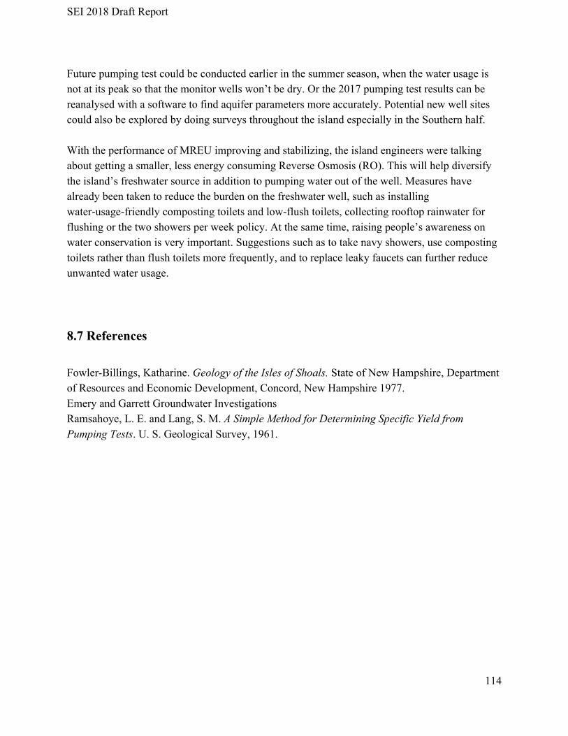
SEI 2018 Draft Report
Future pumping test could be conducted earlier in the summer season, when the water usage is not at its peak so that the monitor wells won’t be dry. Or the 2017 pumping test results can be reanalysed with a software to find aquifer parameters more accurately. Potential new well sites could also be explored by doing surveys throughout the island especially in the Southern half. With the performance of MREU improving and stabilizing, the island engineers were talking about getting a smaller, less energy consuming Reverse Osmosis (RO). This will help diversify the island’s freshwater source in addition to pumping water out of the well. Measures have already been taken to reduce the burden on the freshwater well, such as installing water-usage-friendly composting toilets and low-flush toilets, collecting rooftop rainwater for flushing or the two showers per week policy. At the same time, raising people’s awareness on water conservation is very important. Suggestions such as to take navy showers, use composting toilets rather than flush toilets more frequently, and to replace leaky faucets can further reduce unwanted water usage. 8.7 References Fowler-Billings, Katharine. Geology of the Isles of Shoals. State of New Hampshire, Department of Resources and Economic Development, Concord, New Hampshire 1977. Emery and Garrett Groundwater Investigations Ramsahoye, L. E. and Lang, S. M. A Simple Method for Determining Specific Yield from Pumping Tests. U. S. Geological Survey, 1961.
114