Embed Size (px)
Citation preview

1
CDE May, 2002
Centre for Development Economics
Sustainable Economic Growth for India:An Exercise in Macroeconomic Scenario Building
V. PanditDelhi School of Economics
Fax: 7667159Email: [email protected]
Working Paper No. 100

2
Sustainable Economic Growth for India:An Exercise in Macroeconomic Scenario Building
V. Pandit*
PRESIDENTIAL ADDRESSJanuary 14, 2002
38TH ANNUAL CONFERENCE OF THE INDIAN ECONOMETRIC SOCIETY
Hosted by
MADRAS SCHOOL OF ECONOMICS AND GURU NANAK COLLEGECHENNAI, TAMIL NADU
January 14-16, 2002
In preparing this Lecture I have drawn heavily on a project, recently completed,alongwith Mr. G. Mahanty, for the Institute of Advanced Studies, United NationsUniversity, Tokyo under the Macroeconometric Modelling Project at CDE, supportedalso by the Indian Council of Social Science Research Council, New Delhi and TheIndustrial Development Bank of India, Mumbai. We are indebted to all the threeinstitutions for their financial support. Discussions with Professors K. Krishnamurty, K.Parikh and Y.K. Alagh have been very useful. So have been the suggestions made by Dr.T. Palanivel. S. Raja Sethu Durai of MSE and my students Raghavendra Raju and N.Sundar were extremely helpful in putting together the paper in its present form. Thanksto all.
* Sri Sathya Sai Institute of Higher Learning, Prasanthi Nilayam 515 134. Dist. Anantapur, A.P. and Centrefor Development Economics, Delhi School of Economics, Delhi 110 007.

3
1. Introduction
Use of Macroeconometric models has by now assumed a measure of universality
as an unavoidable aid to forecasting and policy analysis; challenges and controversies
spread over more than two decades notwithstanding.1 While such models are typically
designed and utilised for dealing with short term problems their application to issues of
long term growth has been equally important, though less frequent.2 The present exercise
is intended to examine India’s growth prospects during the first two decades of the third
millennium on the basis of a comprehensive econometric model. The exercise is fairly
straightforward and somewhat traditional. It draws neither upon the growing literature on
“Endogenous Growth” nor upon the recent developments in the econometrics of
“Cointegrated Time Series” which enables one to separate short term from long term
relationships.3
Why we have chosen to follow the traditional and apparently modest line calls for
some explanation. As far as the new theories of growth are concerned it must be pointed
out that our focus in this exercise is at the same time narrower as well as wider than that
of the endogenous growth models. While such models have largely been motivated by
the quest for an explanation for variations in the growth rates of economies across time
and space, our focus is narrowly on the prospects of India’s economic growth over the
next two decades. In any case, in attempting the present exercise one may draw some
comfort from Solow’s Nobel Lecture (see Solow, 2000).
On the other hand, the fact that one is dealing with a poverty ridden developing
economy on the threshold of globalisation, stands in contrast with the mature resilient
industrial economies which modern growth theories are concerned with. For this reason
the focus of our exercise is wider in so far as it is implicitly concerned with the politico-
1 See Pandit (2001).2 Two prominent attempts in this direction have been those by Klein and Kosobud (1961), Behrman and
Klein (1970) and, Hickman and Coen (1976).3 See Barro and Sala-i-Martin (1995) and Aghion and Howitt (1998) on endogenous growth and, Enders
(1995) on modern time series Techniques

4
economic compulsions which are likely to persist at least over the near future. It is the
consequent rigidities and slacks in the economic system which give meaning and
relevance to the question of macroeconomic sustainability of a given pace and structure
of economic growth. Unavoidably, the focus of the exercise has to be wider than that of
theoretical growth models.
As mentioned above, recent developments in time series econometrics provide a
methodology for identifying long run and short run relationships between variables that
are found to be cointegrated. Typically, this methodology is appropriate when one is
dealing with high frequency data sets with an adequately large number of observations.
The fact that we do not have a long enough time series, adequately comparable over time,
considerably erodes the gains associated with this methodology. Two other
considerations are also relevant in this context. First, since our observations are annual,
disequilibrium is unlikely to be a dominent feature of the underlying relationships, even
as its presence may not be totally ruled out. Second, time series modelling, using VAR
or better, SVAR has so far been confined to only simple and small atheoretical models.
Even a moderately sized structural model can turn out to be quite cumbersome under this
methodology.
2. Setting up the Problem
It should be pointed out at the outset that our objective is not to forecast India’s
economic growth over the next two decades. It is, instead, intended to construct a growth
scenario that is attainable and, at the same time sustainable in terms of vital
macroeconomic balances. Criteria of sustainability are dealt with in two ways. While
some are incorporated into the process of growth others are monitored expost as the
growth process follows its own course, to ensure that they remain within limits that are
perceived to be tolerable. The central issue is one of sectoral and overall growth rates
and their implications with respect to macroeconomic equilibrium in a broad sense.
5
The questions under investigation are important because constraints and costs
associated with economic growth need to be clearly understood and evaluated. In
principle, it may be possible for an economy to register a high rate of economic growth
for a while by continually fuelling in larger inputs; which may, in turn generate a variety
of persistent imbalances jeopardising long run growth. The issue then is to identify
growth trajectories consistent with plausible pattern of investment behaviour, and
measures of structural changes including productivity growth, and manageable within a
realistic spectrum of parameters like rate of saving, exchange rate depreciation, external
debt, fiscal balance, and per capita domestic food availability. Clearly, the relative
importance of different constraints and costs would vary from one situation to another
depending on the prevailing economic structure, sociopolitical set up and other relevant
initial conditions.
Some of the foregoing issues have been discussed implicitly as part of the
planning literature in India. But as far as we are aware this literature has been confined to
a five year planning horizon. Even for that, the focus has largely been on the quantum
and allocation of investment consistent with a target growth rate on the one hand and
scope for resource mobilisation on the other. In most cases the methodology used has
consisted of some rules of thumb based on parameters like capital–output ratios. 4
Moreover, the policy regime under which such questions have been posed has
vastly changed during the last decade. Not only the policy implementation set-up but
also the central policy issues have undergone a substantial change. Further changes that
are likely to take place over the subsequent two decades can at best be only guessed at the
moment. These notwithstanding, it is our view that the present study is meaningful in so
far as it caricatures future course of the Indian economy under different alternatives.
Based on a comprehensive econometric model (IEG-DSE, 1999) it is able to handle the
complex issues at hand in a systematic and consistent manner.
4 One exception to this is an exercise undertaken by Krishnamurty, Pandit and Sharma(1989) which has
now become somewhat dated.

6
As stated earlier, the core model in our analysis is fairly simple and consists of
production and investment functions. We assume Cobb-Douglas type production
functions rather then fixed capital-output ratios, as planning exercises have usually done.
Capital formation is posited to follow the accelerator hypothesis with other determinants
like the real rate of interest, and other structural factors characterising developing
economies. This given us the core of the model as:
Yt = F ( Kt-1 { Zt },t )
It = φ ( ∆ Yt-1, Rt - π , CRt )
Kt = ( 1 - δ ) Kt-1 + I t-1
Where Y stands for output, K for capital stock, t for time, {Z} for infrastructure and other
relevant inputs, I for investment, R for nominal interest rate, P for price level, π for
expected rate of inflation CR availability of real credit and δ rate of depreciation. To
ensure that the economy moves along the warranted growth path in the sense of Harrod
(1939), we monitor the balance between saving, investment and capital inflow.
The exercise has been carried out, as stated earlier, on the basis of parts of a
macro-econometric model, (IEG-DSE, 1999) which has served as a reliable system for
short to medium term forecasting and policy analysis for nearly a decade. While some
parts of the model have been dropped or condensed some have been modified to suit the
present purpose of dealing with long term growth. Also, since the model is based on data
for the period 1970-71 through 1996-97 some parameters are modified here and there in
view of perceived structural changes likely to occur in the years to come. The somewhat
detailed submodel dealing with the external sector has been retained as in the original
model.
We build up three scenarios, which are as follows. First, we set up a base line or
"Business as Usual" scenario (A) in which the system follows its own course with built-in
modifications. Then we add a technical progress factor on the industrial sector and
introduce inflow of foreign direct investment at varying rates to augment domestic

7
resources. This gives us scenario (B). From all counts scenario (B) does not appear to be
sustainable in terms of the environmental problems, particularly the maintenance of water
resources. This calls for the third scenario (C) in which a part of the public investment is
used to maintain and / or improve environmental resources rather than to add to the
capital stock in any particular sector.
Thus, we have three scenarios as follows:
A. Baseline or “Business as Usual” scenario.
B. Technical Progress and Inflow of Foreign Direct Investment added on to A or,
the “Globalisation” scenario.
C. A slice of investment diverted from physical capital formation to environ-
mental protection. This modification is superimposed on scenario B, giving us
the “Environmental Protection” scenario.
As mentioned earlier sustainability is partly imposed on the growth process, as
we shall explain subsequently. But more explicitly and perhaps more importantly we
monitor movements of five variables to check sustainability. These are:
I. Public sector resource gap as percentage of GDP
II. Current account balance as percentage of GDP
III. Growth of per capita real consumption expenditure indicating welfare, and,
IV. Growth of per capita availability of food grains as an indicator of the measure
of food security.
V. Economy wide balance between saving and investment.
3. Model Structure and Modifications
The IEG – DSE model5 (now referred to as the CDE - DSE model) which is our
starting point is a large macroeconometric model which deals comprehensively with the
Indian economy. It consists of eight sub models, which add up to nearly 350 equations.
The submodels deal one each with output, capital formation, price behaviour, money and
5 For details see IEG-DSE (1999).

8
banking, public finance, trade and balance of payments, private consumption and savings.
Broadly speaking the structure of the model is as follows. The level of economic activity
is supply driven in case of agriculture and infrastructure and largely demand driven in
case of services. For manufacturing both are important though the balance is somewhat
titled in favour of supply. Modelling of Public Administration and defence is structurally
dictated and as expected, linked with public finance. Price movements are explained in
terms of money stock growth in relation to real output growth, administered prices and
unit value of imports. Prices of food and more broadly agricultural products, which are
an input to other prices, are assumed to be market clearing with fixed supply in the short
run.
Trade flows are disaggregated into four groups as per SITC one digit
classification. The trade sub model is based on the small open economy assumptions so
that all import prices in US dollars are exogenous. On the other hand exports (except in
case of oil which are exogenous) are the outcome of supply – demand interaction. Thus
prices and domestic supply constraints play an important role in export growth
performance, as do the given international market trends. Import volumes are
predominantly determined by the domestic level of activity, which includes overall GDP
growth, level of fixed capital formation and the tempo of industrial growth. In the
present context it is important to underline that a higher rate of economic growth implies
possibly a larger measure of disequilibrium in the external sector. 6
The public finance sub model explains a wide class of fiscal operations including
the financial balances of the public sector undertakings. As expected revenues are
closely related to the level of economic activity, with given fiscal parameters. Money
stock (M3) is determined as the result of equilibrium between supply and demand for the
three components of M3, namely currency, Demand deposits and time deposits in a
complex manner. Monetary policy parameters are built into the money multiplier. The
money - finance submodel also explain prime lending rates of banks and nonbank
6 This has indeed been a prominent result from an earlier exercise (Krishnamurty, Pandit and Sharma,
1989).

9
financial institutions and rates on government securities. Public sector resource gap
influences the last one in a significant way.
As mentioned earlier private fixed capital formation is driven by variants of the
accelerator hypothesis, real credit availability and in some sectors by the phenomenon of
crowding in due to public sector investment. In agriculture lagged relative prices, which
serve as proxies for terms of trade also turn out to be important. The model is highly
nonlinear and dynamic with strong linkages across sectors and within sectors. Its
performance in terms of validation tests over the sample period, biannual forecasts over
the last few year as well as results relating to policy analysis has been fairly good and
compares favourably with those of other models that we know of.
A number of modifications have been made in the model, as stated earlier, to
render it not only suitable to the problem at hand but also manageable. In addition, some
constraints have also been imposed on the movement of several variables, which are free
to adjust endogenously in the original model. These modifications and constraints have
been imposed to obtain the baseline solution and retained in all other subsequent
solutions, to ensure comparability across different solutions.
First and foremost, since we are primarily concerned with long term growth
major causes of short run fluctuations need to be curtailed. To this effect we suppress the
structural submodel relating to price behaviour. However, prices are not held constant.
Instead, all domestic prices are assumed to grow secularly at 3 percent. This means a
kind of steady state in which the inflation rate is fixed and all relative prices are frozen.
Second, following from the above, since prices are largely influenced by monetary -
financial variables, the submodel relating to money stock, interest rates etc. is eliminated
from the model. We do however assume domestic credit to grow at rates, which are not
far from those that have prevailed over the recent past. We also set major interest rates at
a level such that the real interest rate is about 7 percent. This is arbitrary but apparently

10
plausible. Third, abandoning the five sector set up in the original model we now
disaggregate the economy into nine sectors. 7
Value added is largely explained in terms of capital stock and some crucial inputs
like energy while all pure demand variables are eliminated. With regard to agriculture
we note that for about 12 years the weather conditions have been normal or better than
normal. Since seven of these years of bountiful weather conditions belong to the sample
period the estimated equation for this sector tends to overstate output and growth rates for
agriculture. To rectify this, we give the production function for this sector a negative
boost of 1 percent per annum. Private capital formation, in most cases follows the
accelerator model together with, in some cases, public sector investment and the real rate
of interest. While the accelerator formulation gives rise to mild cyclical variation, the
crowding - in phenomenon also shows up significantly in some cases.
In dealing with the external sector we expect that export growth in volume would
be better than what it has been during the seventies and the eighties. The so posited
structural shift is in keeping with experience over the last few years. In view of this we
modify the equations relating to real exports of manufactures so as to ensure that the rate
of growth of this variable is one percent over and above what it would have otherwise
been. Clearly this is a mild shift in the overall setting.
No modification is made to any of the import functions. Also, we let the nominal
exchange rate (rupees per US dollar) to increase over the two decades by approximately 2
percent annually. Given that domestic prices rise by 3 percent and world prices by 2
percent, this implies that the real exchange rate (dollars per rupee) depreciates by 1
percent approximately.
7 These include agriculture and allied activities (AFF), mining and quarrying (MAQ), manufacturing
(MAN), construction (CON), electricity, gas and water supply (EGW), trade, hotels and restaurants (THR),
transport storage communications(TSC), finance, insurance and real estate (FIR), social community and
other services (SCS).

11
4. Characterising the Alternative Scenarios
With the modifications in the underlying model as explained earlier, the baseline scenario
is generated on the following assumptions:
(a) Domestic inflation rate is fixed at 3 percent per annum. Nominal non-agricultural
non-food credit is assumed to increase at 15 percent per annum. Nominal exchange
rate (rupees per dollar) increases at 3.5 percent per year. This clearly implies
efficient short-term management of monetary and exchange rate policies as a
precondition necessary for the growth scenario.
(b) Public sector comprising of central and state governments and PSUs generate
annually savings equal to 1.5 percent of GDPMP. This is lower than the rate
observed in recent years. But consistent with higher GDP growth and overall
reduction in size of the public sector. Since, no changes are imposed on revenue
collections, the implicit assumption is that reduced tax rates should widen tax base
and be accompanied by better tax compliance.
(c) Public sector capital formation in real terms is set at 7 percent of real GDPMP over
the five years 2000-01 through 2004-05. The ratio declines to 6 percent over the
remaining years. This is allocated to the nine sectors as follows: agriculture and
allied activities (7%), mining and quarrying (10%), manufacturing (8%), construction
(2%), electricity, gas and water supply (25%), trade hotels and restaurants (2%),
transport storage and communications (20%), finance, insurance and real estate (6%),
social, community and other services (20%).
(d) In agriculture net area sown is assumed to remain constant so that greater output
comes from multiple cropping and higher yields. Also, nominal credit to agriculture
grows by about 10 percent per annum.

12
(e) With regard to the international economy it is assumed that world exports in current
US dollars increase at 8 percent over the period 2000 through 2005 and by 6 percent
subsequently. World prices are posited to increase at 2.0 to 2.5 percent in current
dollars. We also assume that the level of economic activity in the Middle East grows
steadily at 4 percent per annum. These figures are broadly consistent with forecasts
made by World Bank, IMF and the World Project LINK.
For the second scenario we add a productivity shock to the two sectors namely
manufacturing and, electricity, gas and water supply. The productivity increase curve is
concave which rises for a while and then declines implying diminishing return to R&D.
As explained earlier the productivity shock is added on to the base line scenario. In
addition we allow for inflow of foreign direct investment amounting initially to US $3
billion, then increasing to $ 5 billion and then topping off at $ 7 billion. By 2015 the
quantum of FDI inflow diminishes back to $ 5 billion and $ 3 billion. Thus, on the one
hand, total capital formation increases and on the other the capital account of the external
sector gets altered. FDI is allocated largely to manufacturing and infrastructure sectors.
Finally, the environment protection scenario assumes that given the total public
sector real investment part of it (1.5 percent of real GDP) goes to the maintenance and
improvement of environment. This gives us the third scenario under which there is a
decline in output levels and growth rates as expected. Thus, we have a situation of trade-
off between higher consumption of goods and services and the quality of life. However,
one may eventually visualise the latter to raise productivity so that the trade-off margin
improves in favour of environmental protection.
Chart 1 : Productivity Curve
0.05
0.10
0.15
0.20
0.25
0.30
2003
2005
2007
2009
2011
2013
2015
2017
2019
2021
2023
2025
2027
2029

13
Sustainable Growth Scenarios
In keeping with the standard methodology we simulate the model incorporating the
modifications and assumptions described earlier for the 25 year period, 1995-96 through
2019-2020. A five year lead was necessary because the model having been estimated
with old national accounts data (base 1980-81) had to be solved with initial conditions
provided by the same data base. It must be noted that absolute values given by the
simulation exercise will not in many cases be close to the actual values in recent years.
This is partly because of the above mentioned data base and partly because of the tempo
and pattern of movements imposed on certain variables, e.g., the level of prices, are
different from the actual. In this section we shall focus only on summary results relating
to important variables.8
Before we turn to these results let it be recalled that the baseline scenario A which
is termed “Business as Usual” consists of solutions to the modified model as it stands .
Under scenario B which is termed “Globalisation” we add foreign direct investment and a
technological change factor for different sectors to scenario A. Results corresponding to
the two factors have been worked out separately but here we report them together. Under
scenario C which is termed “Environment Protection” it is envisaged that a part of the
public sector investment amounting to 1.5% of GDP is diverted to maintenance and
improvement of the environment rather that to physical capital formation.
To render the task of comparison and interpretation manageable the nine sectors
of economic activity are collapsed into three, namely, agriculture, industry and services.
Again, rather that reporting results on a year to year basis we either report averages for
selected periods or for selected years. All movements are to be seen as being long or
medium run in character. This is because many segments of the model generating short
run movements have been eliminated and many variables are subjected to only long run
8 Solution values of these variables are given in Appendix B on an annual basis.

14
trends. Finally, it bears a repetition to say that the present excersise is not about
forecasting but about scenario building.
5.1. Output Growth
First of all, we observe mild cyclical pattern in the annual growth rates of total GDP
under all scenarios. (See graph). This is clearly due to the dynamic non-linear character
of the model. However, since the year to year deviations are not too large averaging over
years has no distortionary effects. Table 1 below gives us sectoral and total GDP growth
rates averaged over four year periods for the three scenarios. It is clear that the highest
rates of growth are recorded under scenario B for all sectors for each period, almost.
Under this scenario the level of output in the year 2019-20 is nearly 4.3 times as much as
it is in the year 2000-01. Under scenarios A and C the corresponding figures are
approximately 3.6 and 3.5 respectively.
Two things need to be noted from our results. First, under both baseline scenario
as well as scenario B rate of annual growth in agriculture is close to or above 5 per cent.
There is reason to believe that this is not sustainable in terms of the demand it will make
on water resources and more generally on the state of the environment9. Second, there is
a trade-off between environment protection and growth over a medium run. But, over a
longer run better environment should at least partly, help to maintain productivity growth
which we do not take into account. If this is kept in mind the balance of trade-off would
tilt in favour of investment in environment.
As expected, the impact of technology accelerates the GDP growth by about half
a percentage point over the first five years and by about three quarters of a percentage
point over the next fifteen years. Over the next quinquinnium the difference is very
small. The effect of FDI is similarly spread. But the major impact on growth rates is
confined to half a percentage point. It is necessary recall that the assumed productivity
shock itself is rather mild and curved to ensure sustainability. If we consider only the
technology shock scenario with the baseline 68 percent of the increase in output between
9 On this see Bhalla et. al (1999).

15
2000 and 2020 comes from investment and 32 percent from productivity. But if we take
up all the three scenarios together the contribution of capital formation is about 59
percent, productivity 29 percent and FDI about 12 percent. As noted earlier concern for
environment has costs. Annual growth rate declines marginally from 7.3 percent to 7.2
percent over 2012-16 and more significantly from 7.3 percent to 7.0 percent over 2016-
20. Over the earlier period the differences are rather small.
Table 1Growth Rates of Sectoral and Total GDP
(4-year averages: percent)
Agriculture IndustryPeriodScenarioA
ScenarioB
ScenarioC
ScenarioA
ScenarioB
ScenarioC
2000-2004 3.25 3.37 2.46 6.45 7.79 6.672004-2008 4.55 4.83 3.66 6.01 7.71 6.502008-2012 4.73 5.18 3.76 8.21 9.61 8.532012-2016 5.73 5.95 4.35 8.29 9.20 7.972016-2020 5.35 6.09 4.17 8.10 8.54 7.05
Services Total GDP2000-2004 6.72 7.51 6.47 5.87 6.74 5.922004-2008 6.61 7.71 6.77 5.97 7.17 6.082008-2012 7.03 8.38 7.39 7.06 8.33 7.232012-2016 7.18 8.57 7.37 7.32 8.43 7.162016-2020 8.23 9.51 7.90 7.73 8.62 7.04
In terms of US Dollars nominal GDP is approximately four and a half times its
initial level under scenarios A and C and, five and half a times under scenario B. As
expected, increases in per capita terms are of lower order (table 2)
Table 2Nominal GDP in U.S Dollars (GDP$)
(1999-00: Scenario A = 100)
Total GDP $ Per Capita GDP $YearScenarioA
ScenarioB
ScenarioC
ScenarioA
ScenarioB
ScenarioC
1999-00 100.0 100.8 99.2 100.0 100.7 99.32003-04 128.5 133.7 126.9 120.1 124.9 118.62007-08 169.4 184.6 168.2 148.0 161.2 147.02011-12 231.2 264.5 231.6 189.2 216.4 189.52015-16 320.0 382.0 319.6 245.7 293.4 245.52019-20 451.7 557.5 440.9 325.9 402.2 318.1

16
5.2 Sectoral Composition of Output and Capital-Output Ratios
Table 3 below gives the levels of value added in the three sectors by quinquinnial
averages and their shares in total GDP. It is clear that under scenario A changes in the
composition of output are not very sharp. Increase in the share of services is not very
sharp even under scenarios B and C. By implication the shift is largely confined to that
between agriculture and industry. The share of agriculture which is around 20 per cent
in the first quinquinnium declines to about 15 per cent under A and B but more sharply to
about 12.5 per cent under C. The share of industry which stands around 40 per cent rises
marginally by about 1.5 percentage points under A, but by over 3 percentage points under
B and nearly 4 percentage points under C.
Finally, a few comments on the productivity of capital. In table 4 below we report
average and incremental capital-output ratios for the three sectors and the economy by
quinquinnial averages. It is necessary to look at the movements in these ratios over the
two decades under the three alternative scenarios to ensure that outcomes under
alternative scenarios are plausible. One thing that stands out sharply is that the capital
output ratio rises for agriculture10 whereas it falls for both industry as well as services.
This is true of averages as well as incremental capital output ratios. Once again changes
are sharper under scenario C than those under scenarios A or B.
10 This is consistent with the view of Bhalla et al. (1999) that further growth of food grains production willrequire heavier investments. On this also see Gulati and Bathla(2001)

17
Table 3
Level and Composition of Sectoral Output: Quinquinnial Averages(Billion 1980-81 Rupees)Year/Scenario Agriculture Industry Services GDPScenario A2001-05 834.92 1638.68 1639.58 4113.17
(20.35) (39.80) (39.85) (100.00)2006-10 1037.46 2332.89 2316.69 5687.04
(18.30) (41.00) (40.70) (100.00)2011-15 1314.38 3288.36 3341.04 7943.78
(16.58) (41.40) (42.02) (100.00)2016-20 1708.14 4625.17 4908.11 11241.42
(15.24) (41.16) (43.60) (100.00)Scenario B2001-05 840.75 1733.55 1695.71 4270.02
(19.78) (40.52) (39.70) (100.00)2006-10 1063.14 2680.56 2531.18 6274.88
(17.03) (42.67) (40.31) (100.00)2011-15 1387.84 4122.24 3891.23 9401.31
(14.81) (43.83) (41.36) (100.00)2016-20 1874.51 6135.39 6027.19 14037.09
(13.40) (43.73) (42.87) (100.00)Scenario C2001-05 806.81 1658.58 1629.36 4094.75
(19.78) (40.44) (39.78) (100.00)2006-10 964.96 2462.48 2333.88 5761.32
(16.83) (42.69) (40.48) (100.00)2011-15 1174.75 3644.13 3443.02 8261.91
(14.27) (44.09) (41.64) (100.00)2016-20 1464.49 5185.82 5062.80 11713.11
(12.55) (44.28) (43.17) (100.00)Note: Figures in bracket denote shares(percent)

18
Table 4Capital Output Ratio*
Year/Scenario Agriculture Industry Services TotalScenario A2001-05 1.38
(1.63)2.79(2.51)
1.86(1.44)
2.13(1.95)
2006-10 1.44(1.78)
2.67(2.31)
1.71(1.30)
2.05(1.80)
2011-15 1.53(1.84)
2.51(2.30)
1.56(1.18)
1.95(1.61)
2016-20 1.62(2.07)
2.36(1.99)
1.42(1.11)
1.84(1.57)
Scenario B2001-05 1.39
(1.64)2.91(2.82)
1.85(1.42)
2.19(2.12)
2006-10 1.45(1.77)
2.81(2.52)
1.68(1.28)
2.12(1.91)
2011-15 1.54(1.82)
2.62(2.13)
1.51(1.17)
2.00(1.68)
2016-20 1.63(1.99)
2.41(1.91)
1.37(1.11)
1.86(1.53)
Scenario C
2001-05 1.37(1.65)
2.83(2.66)
1.84(1.35)
2.15(2.02)
2006-10 1.43(1.84)
2.72(2.40)
1.66(1.20)
2.07(1.83)
2011-15 1.52(1.91)
2.54(1.98)
1.49(1.07)
1.95(1.57)
2016-20 1.62(2.29)
2.31(1.68)
1.33(0.99)
1.80(1.39)
*Numbers in parentheses are incremental capital outputratio
5.3 Sustainability
Having checked the plausibility of the different growth scenarios let us now turn to the
question of sustainability in terms of the four measures discussed in section 1. These
consists of fiscal balance, measured in terms of overall public sector resource gap (RG),
external balance measured by trade deficit as a proportion of GDP (EB), food security
measured by per capital availability of domestically produced foodgrains (FG) and finally
growing levels of living measured as per capita real consumption expenditure (CON).
These are reported below.
19
Table 5Public Sector Resource Gap
(Percent of GDP )
Year ScenarioA
Scenario B ScenarioC
1999-00 5.4 5.4 3.72003-04 6.0 6.0 4.32007-08 6.4 6.5 4.72011-12 5.7 5.8 4.02015-16 6.0 6.1 4.32019-20 6.3 6.4 4.5
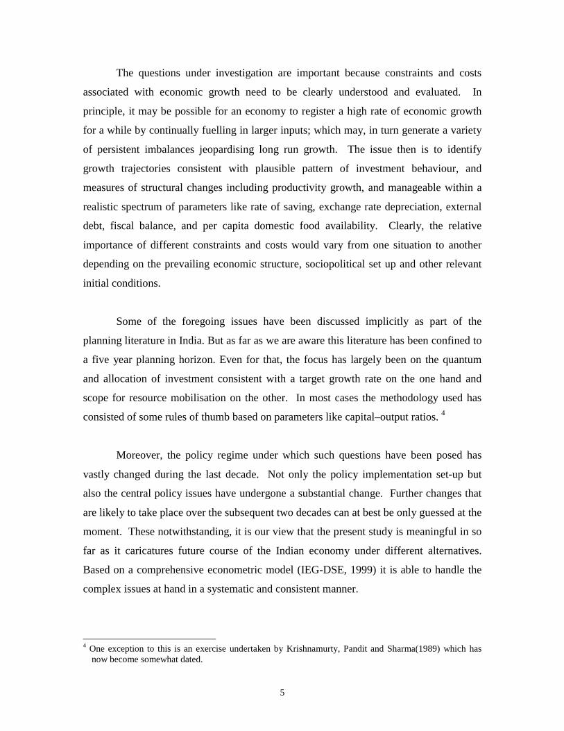
At the outset we need to note that RG is important in so far as we assume that
public sector investment in agriculture and infrastructure would remain significant even
as the share of such investment in total GDP would keep declining. Our calculations
given in table 5 show that under scenarios A and B RG remains close to or mostly above
6 percent of GDP. In a sharp contrast, however the ratio drops to a level below 5 under
scenario C.
Similarly EB is unmanageably high under both scenarios A and B. It is extremely
high particularly under scenario B. Again, in contrast under scenario C the imbalances is
not only within manageable limit all along but even negative in the terminal year. Thus,
if invisibles are assumed to be of the order of 2 to 3 percent of GDP, current account
deficit will be close to 2 percent of GDP except in 2003-04. The interesting feature of the
external imbalance is its sharp decline towards the end of the second decade. Finally we
note that under all scenarios rates of saving remain marginally above the rates of saving
remain marginally above the rates of investment (Table 7) indicating the possibility if
higher growth rate as far as savings are concerned.

20
Table 6Trade Balance as Proportion of GDP
Year ScenarioA
ScenarioB
Scenario C
1999-00 -4.91 -5.34 -4.082003-04 -7.15 -9.18 -6.282007-08 -6.14 -7.93 -5.242011-12 -6.80 -12.55 -5.252015-16 -7.59 -19.06 -3.182016-20 -5.97 -21.38 4.79
Table 7Rate of saving and Investment
Year 2003-04 2007-08 2011-12 2015-16 2019-20Rate ofSaving
32.5 31.8 33.7 34.0 34.9
Rate ofInvestment
30.8 30.9 31.0 31.6 32.0
Turning now to the measures of well being we note that, over the twenty year
period per capita real consumption expenditure multiplies by 2.61 under scenario A, by
3.93 under scenario B and by 3.21 under scenario C. At the end of the period per capita
consumption expenditure reaches Rs. 6677.36 billion at 1980-81 prices. In dollar terms
per capita private nominal consumption expenditure rises over the two decades from
about $200 to about $726. Table 8 below gives rates of increase over quinquinnial
periods.
In dealing with food security we need to note that our projections run in terms of
total quantum of foodgrains. Many others, notably Bhalla et.al. (1999) have dealt with
availability of cereals rather than total foodgrains. Also, since cereals are partly to be
used for feed and seed we need to consider net availability for human consumption.

21
Needless to say that the feed part is going to go up in future. Going by the figures used
by Bhalla et.al. and the fact that cereals usually account for 90 percent of foodgrains, net
availability of cereals available for human consumption would be about 318 million
tonnes by our projection. This is adequate to meet the demand of 254.5 Million tonnes
projected by Kumar (1998). Finally, though these different figures appear to be of
similar magnitude they are not strictly comparable due to differences in the methodology
used.
Table 8Growth Rates of Per Capita Consumption Expenditure
and Output of Foodgrains(Percent per year)
Consumption Expenditures Production of FoodgrainPeriodScenarioA
ScenarioB
Scenario C ScenarioA
ScenarioB
ScenarioC
2001-05 4.48 5.56 4.62 2.89 3.15 2.002006-10 5.21 6.76 5.81 3.80 4.38 2.852011-15 5.40 7.10 6.07 4.66 5.47 3.722016-20 6.03 7.22 5.86 4.68 5.71 3.60
Table 9 gives per capita production availability under scenarios A and C, averaged over
quinquinnial stretches.
Table 9Output and Availability of Food Per Capita
(Kg: Average)
Foodgrains Cereals Net Availability ofCereals
Period ScenarioA
ScenarioC
ScenarioA
ScenarioC
ScenarioA
ScenarioC
2001-05 216.4 208.3 194.7 187.5 155.8 150.02006-10 264.5 243.2 238.0 218.8 190.4 175.12011-15 328.9 287.3 296.0 258.6 236.8 206.92016-20 419.7 348.7 377.8 313.8 302.2 251.1

22
5. Summing Up
With the onset of the final decade of the last century (and the Millennium!) India
explicitly adopted a new economic policy regime – departing from the path that had been
followed for the preceding four decades. It may be premature to construct a view of the
two next decades yet it is tempting to anticipate what might be desirable and feasible.
This is what the present study tries to do. Clearly and unavoidably an exercise of this
kind has to be based on a number of speculative assumptions. Thus, it is clear that what
we attempt to build ultimately is a growth scenario that is attainable and sustainable in its
various macroeconomic dimensions. Under more favourable conditions economic
growth might be more impressive.
Using a formal macroeconomic model with suitable modifications and
assumptions built into it we try to project how the different sectors are likely to grow over
the first quarter century of the new millennium. While some of the feasibility norms like
inflation rates and rates of currency depreciation are built into the model itself some
others are monitored expost to ensure sustainability. These include fiscal balance, which
has turned out to be important under the new policy dispensations, overall resource
balance external equilibrium, levels of living and food security. These are respectively
measured by public sector’s overall resource gap, saving-investment tally current account
deficit, both as ratios of GDP, per capita real consumption expenditure and per capita
availability of foodgrains / cereals.
Finally, we have paid an explicit attention to environmental problems, which are
bound to multiply with growth. We also assume a pragmatic growth in productivity and
inflow of foreign direct investment. The sustainable scenario that emerges ultimately is
the one we call “Enviornment Protection”. It points to a growth rate around 7 per cent,
with share of agriculture going down to 12.5 per cent and capital output ratio converging
to about 1.8. Real GDP per capita in 1919-20 is a little more than thrice as much as in
2000-01. A similar increase also takes place in per capita consumption. It is clear that
lower growth recorded under the sustainable scenario, may overstate the trade-off

23
between environmental quality and consumption. In any case our results are in line with
those mentioned by Solow (2000) on the basis of Dennison’s calculations for the US
economy. Among other factors investment in environment may lead to lower “measured”
output growth.
External deficit goes beyond the tolerable limit for a while but ultimately comes
down to a level below the 2 per cent norm. Fiscal gap drops slowly and remains close to
4 per cent of GDP. The most important result we get is that a rate of growth of real GDP
above 7 per cent is not sustainable; nor so is agricultural sector’s growth above 4 percent.
It is necessary to add that an implicit assumption underlying the exercise is good
macroeconomic management and normal weather conditions. Given the nature of the
exercise there is no explicit role for micro economic changes in the economy nor for the
way social sectors go. Nevertheless, the presumption is that unemployment, poverty and
inequality and other vital socioeconomic indicators do not worsen so as to cause systemic
failures.
24
References
Aghion P. and P Howitt (1998), Endogenous Growth Theory, Cambridge, Mass. TheMIT Press.
Ahluwalia, I.J. and I.M.D. Little, eds, (1998), India’s Economic Reforms andDevelopment: Essays for Manmohan Singh, Delhi, Oxford University Press.
Barro, R. and Xavier Sala-I-Martin (1995), Economic Growth, New York, Mc Graw Hill.
Behrman, J. R. and L. R. Klein (1970) Econometric Growth Models for the DevelopingEconomy, in W. A. Eltis, M. F. G. Scott and J. N. Wolfe (eds.) Induction,Growthand Trade, London, Oxford University Press.
Bhalla, G.S. Peter Hazel and John Kerr (1999), Prospects for India’s Cereal Supply andDemand to 2020, Washington, International Food Policy Research Institute, Food,Agriculture and the Environment, Discussion Paper No. 9.
Bhattacharya, B.B., R.B Burman and A.Nag (1994), Stabilisation Policy Options: AMacroeconometric Analysis, Mumbai, DEAP Reserve Bank of India, DRG StudyNo. 8.
Bhide, S., A. Sinha, S. Pohit and D. Joshi (1996), Macroeconomic Modelling forForecasting and Analysis, National Council of Applied Economic Research, NewDelhi and Conference Board of Canada.
Chakravarty, S. (1987), Development Planning: The Indian Experience, Delhi, OxfordUniversity Press.
Chitre, V.S. (1992), Crisis in the Indian Economy : Issues and Policy Options, in V.R.Panchmukhi, ed., Fiscal Management of the Indian Economy, Delhi, InterestPublications.
Enders, W.(1995), Applied Econometric Time Series, New York,John Wiley.
Gulati, Ashok and Seema Bathla(2001), Capital Formation in Indian Agriculture:Revisiting the Debate, Economic and Political Weekly, May 19, 2001.
Harrod, R.F. (1939), An Essay in Dynamic Theory, Economic Journal, March .
Hickman B. and R Coen (1976), An Annual Growth Model for the US Economy,Amsterdam, North Holland.
IEG - DSE (1999), Policies for Sability and Growth: Experiments with a Large andComprehensive Structural Model for India, Journal of Quantitative Economics,

25
Special Number on Macroeconomic Policy Modelling edited by V. Pandit andK.Krishnamurity, Vol. 15, No.2.
Jalan, B. (1991), India’s Economic Crisis: The Way Ahead, New Delhi, Penguin.
Klein, L.R.(1971), Forecasting and Policy Evaluation Using Large Scale EconometricModels : State of the Art, in M.D. Intrilligator (ed). Frontiers of QuantitativeEconomics, Amsterdam, North Holland.
Klein, L. R. and R. F. Kosobud (1961) Some Econometrics of Growth: Great Ratios ofEconomics, Quarterly Journal of Economics, May.
Krishnamurty K. and V.Pandit (1996), Exchange Rate, Tariffs and Trade Flows:Alternative Policy Scenarios for India, Indian Economic review, Vol. 31, No. 2,Reprinted in Journal of Asian Economics, Vol. 8, No.3.
Krishna, K.L., K. Krishnamurty, V.Pandit and P.D. Sharma (1991), MacroeconometricModelling in India: A Selective Review of Recent Research, in EconometricModelling and Forecasting in Asia, Development Papers No. 9, Bangkok,ESCAP, United Nations.
Krishnamurty, K., V. Pandit and P.D. Sharma (1989), Parameters of Growth in aDeveloping Mixed Economy: The Indian Experience, Journal of QuantitativeEconomics, Vol. 5 No. 2.
Kumar, P.(1998), Food Demand and Supply Projections for India, AgriculturalEconomics Policy Paper 98-01, Indian Council of Agricultural Research Institute,New Delhi.
Pandit, V. (1993), Controlling Inflation: Some Analytical and Empirical Issues,Economic and Political Weekly, January 2-9.
Pandit, V. (1999), Macroeconometric Policy Modelling for India; A Review of someAnalytical Issues, Journal of Quantitative Economics, Special Number, Vol.15,No 2.
Pandit, V. (2001), Structural Modelling Under Challenge, Working Paper No. 98, CentreFor Development Economics, Delhi. (Invited Lecture to the 37th AnnualConference, The Indian Econometric Society, South Gujarat University, Surat,April 13-15, 2001.
Pandit V., K. Krishnamurthy and T. Palanivel (1995), Gazing the Crystal Ball: IndianEconomy, Circa 1995, Economic and Political Weekly, May 6-13.
Rangarajan, C. (2000), Perspectives on Indian Economy, New Delhi, UBS Publishers.

26
Solow, Robert (1956) A Contribution to the Theory of Economic Growth, QuarterlyJournal of Economics, Vol. 70, No. 1.
Solow, Robert (2000) Growth Theory, 2nd edition, New York, Oxford University Press.

27
APPENDIX ACore Structural Linkages
In this appendix we give some of the critical relationships which form a part of
the core model in so far as they determine the growth process. To this effect we report
three sets of equations, most of which are estimated. These include (a) production
functions (b) investment functions and (c) other critical relationships. In particular, we
need to understand how these are specified in order to identify important linkages in the
model and also to assess their statistical characteristics. The complete model including
the large number of accounting
identities and assumed trend curves are given in Annexure C.
It needs to be underlined that we have deliberately confined to the somewhat short
sample period beginning with 1980-81, in order to minimise inaccuracies due to the
change in the policy regime. The presumption is that data for the earlier period would
not be relevant for capturing the emerging future relationships. How far we may remain
off the track, nonetheless, only future will tell.
A.1 Production Functions
In almost all cases we try to explain output capital ratio. Two major exceptions are
agriculture where we look at output per unit of area under cultivation and manufacturing
for which the dependent variable is directly the level of output. In addition to the nine
sectoral production functions we also have a function explaining the gross output of
foodgrains, in view of its special role. One common explanatory variable in most cases is
the level of infrastructure. Judged by the usual diagnostics all estimated relationships are
fairly good. In particular, there is no evidence of serial correlation. Only, the sample
period of 1980-81 through 1994-95 is rather short, something one cannot help.
1. Agriculture, fishing & forestry
LOG(ZAFF) = -3.529 + 0.936 LOG (ZNSAFF(-1) + 0.797 LOG(IAAC)

28
(-1.431) (9.534) (1.358)
+ 0.024 DUMRAC + 0.074 D90T97 + 0.067D76
(2.067) (2.786) (1.660)
SAMPLE PERIOD: 1975-97 R2 = 0.96 DW= 1.66
2. Mining & quarrying
LOG(ZMQ/ZNSMQ(-1)) = -2.038 + 0.877 LOG (ZNSMQ(-1))
(-1.488) (1.541)
+1.856 LOG(ZEGW/ZNSMQ(-1)) –0.093TIME
(3.075) (-1.988)
SAMPLE PERIOD: 1981-97 R2 = 0.95 DW= 1.57
3. Manufacturing
LOG(ZMN) = 0.333 + 0.219 LOG(ZNSMN(-1)) + 0.553 LOG(ZEGW)
(0.504) (1.850) (5.471)
+ 0.331 LOG(ZAFF) -0.099D92345
(2.803) (-8.041)
SAMPLE PERIOD: 1981-97 R2 = 0.99 DW= 2.29
4. Electricity, gas & water supply
LOG(ZEGW/ZNSEGW(-1)) = -0.227 – 0.459 LOG (ZNSEGW(-1))
(-0.360) (-3.603)
+ 0.043 TIME
(4.710)
SAMPLE PERIOD: 1981-97 R2 = 0.94 DW= 1.64
5. Construction
LOG(ZCONS/ZNSCON(-1)) = 2.463 – 0.471 LOG (ZNSCON(-1))
(11.124) (-7.244)
+ 0.700 LOG(ZEGW/ZNSCON(-1)
(7.356)

29
SAMPLE PERIOD: 1981-97 R2 = 0.79 DW= 1.54
6. Trade, hotels & restaurant
LOG(ZTHR/ZNSTHR(-1)) = 0.427 + 0.069 LOG (ZNSTHR(-1))
(3.082) (2.312)
- 0.062 D92 + 0.129 D9697
(-2.418) (5.711)
SAMPLE PERIOD: 1981-97 R2 = 0.85 DW= 1.83
7. Transport, storage & communication
LOG(ZTSC/ZNSTSC(-1)) = -0.854 + 0.111 LOG (ZNSTSC(-1))
(-1.352) (1.509)
+ 0.538 LOG(ZEGW/ZNSTSC(-1)) + 0.056D75T91 – 0.022D95
(5.961) (4.280) (-1.604)
SAMPLE PERIOD: 1981-97 R2 = 0.97 DW= 2.11
8. Finance, insurance, real estate & business services
LOG(ZFIRB/ZNSFIR(-1)) = -2.960 + 0.470 LOG (ZNSFIR(-1))
(-7.905) (11.180)
+ 0.598 LOG(ZEGW/ZNSFIR(-1)) – 0.031D93
(21.308) (-3.406)
SAMPLE PERIOD: 1981-97 R2 = 0.99 DW= 1.92
9. Community, social & personal services
LOG(ZCSPS/ZNSCSP(-1)) = -3.435 + 0.696 LOG (ZNSCSP(-1))
(-3.250) (3.517)
+ 0.512 LOG(ZEGW/ZNSCSP(-1)) – 0.037TIME
(2.889) (-2.942)
SAMPLE PERIOD: 1981-97 R2 = 0.97 DW= 1.73

30
Production of Foodgrains
LOG(FGRAIN) = -0.988826542 + 0.947256175*LOG(ZAFF)
(-5.26) (31.88)
SAMPLE PERIOD: 1975-97 R2 = 0.98 DW= 1.57
A.2 Private Capital Formation
In explaining private capital formation at sectoral levels we have largely followed the
accelerator hypothesis and supplemented it by some other explanatory variables like the
real rates of interest, availability of credit, rates of inflation, and the level of public
sector’s real capital formation in the particular sector under consideration. The last
variable is believed to capture the crowding in/out phenomenon. Outliners have been
taken care of by means of dummy variables. Unlike in case of production functions we
have been able to extend the sample period up to 1995-96.
Agriculture, fishing & forestry
ZGIAFFPV = -79..891 + 0.089 ZAFF(-1) + 0.072 ZAFF(-2)
(-3.888 (2.554) (1.942)
+ 1.479ZGIAFFPU + 5..653(ZTAC-ZTAC(-1))
(2.233) (0.376)
SMALPE PERIOD: 1981-1996 R2 = 0.89 DW= 1.98
2. Mining & Quarrying
ZGIMQPV = -0.944 + 0.566 (ZMQ-ZMQ(-1)) + 0.058 ZGIMQPU
(-2.191) (4.630) (3.336)
-2.229 D899091 + 2.949 D83
(-5.517) (5.505)
SAMPLE PERIOD: 1981-96 R2 = 0.86 DW= 1.66
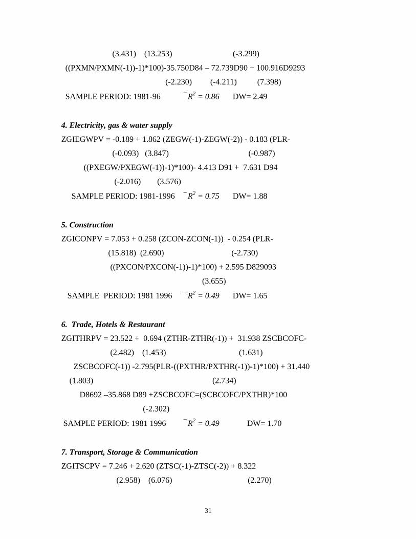
3. Manufacturing
ZGIMNPV = 63.378 + 3.045 (ZMN-ZMN(-1)) – 6.922 (PLR-
31
(3.431) (13.253) (-3.299)
((PXMN/PXMN(-1))-1)*100)-35.750D84 – 72.739D90 + 100.916D9293
(-2.230) (-4.211) (7.398)
SAMPLE PERIOD: 1981-96 R2 = 0.86 DW= 2.49
4. Electricity, gas & water supply
ZGIEGWPV = -0.189 + 1.862 (ZEGW(-1)-ZEGW(-2)) - 0.183 (PLR-
(-0.093) (3.847) (-0.987)
((PXEGW/PXEGW(-1))-1)*100)- 4.413 D91 + 7.631 D94
(-2.016) (3.576)
SAMPLE PERIOD: 1981-1996 R2 = 0.75 DW= 1.88
5. Construction
ZGICONPV = 7.053 + 0.258 (ZCON-ZCON(-1)) - 0.254 (PLR-
(15.818) (2.690) (-2.730)
((PXCON/PXCON(-1))-1)*100) + 2.595 D829093
(3.655)
SAMPLE PERIOD: 1981 1996 R2 = 0.49 DW= 1.65
6. Trade, Hotels & Restaurant
ZGITHRPV = 23.522 + 0.694 (ZTHR-ZTHR(-1)) + 31.938 ZSCBCOFC-
(2.482) (1.453) (1.631)
ZSCBCOFC(-1)) -2.795(PLR-((PXTHR/PXTHR(-1))-1)*100) + 31.440
(1.803) (2.734)
D8692 –35.868 D89 +ZSCBCOFC=(SCBCOFC/PXTHR)*100
(-2.302)
SAMPLE PERIOD: 1981 1996 R2 = 0.49 DW= 1.70
7. Transport, Storage & Communication
ZGITSCPV = 7.246 + 2.620 (ZTSC(-1)-ZTSC(-2)) + 8.322
(2.958) (6.076) (2.270)

32
D(SCBCOFC/PXTSC) -6.121D8687 + 6.999 D929394
(-2.794) (3.333)
ZSCBCOFC=(SCBCOFC/PXTSC)*100
SAMPLE PERIOD: 1981 1996 R2 = 0.49 DW= 2.19
8. Finance, insurance & real estate & business services
ZGIFIRPV = 23.734 + 1.929 (ZFIR(-1)-ZFIR(-2)) – 0.616(PLR-
(4.147) (9.246) (-1.149)
((PXFIR/PXFIR(-1))-1)*100) + 26.759 D9496
(5.618)
SAMPLE PERIOD: 1981 1996 R2 = 0.91 DW= 2.09
9. Community, social & personal services
ZGICSPPV = -5.604 + 0.223 ZGICSPPU + 0.655 ZGICSPPV (-1)
(-4.300) (4.448) (3.859)
SAMPLE PERIOD: 1981 1996 R2 = 0.88 DW= 1.75
A.3 Other Structural Relationships
In this set of relationships we include volumes supply and demand for exports of
manufactured goods, the latter normalised in terms of the unit value index, imports
demand for manufactures and POL products. But before we report these it is useful to
indicate that in building sustainable growth scenarios we match the quantum of investible
resources ( R) against total investment. R is calculated as follows:
R = S + FDI + AID + OT - CR
Where S denotes domestic saving, FDI foreign direct investment, AID external aid, OT
other capital account transfers and CR increase in foreign exchange reserves.
Merchandise Real Exports
SITC : 5 to 9 (DGCI&S)
LOG(ZEX59) = 1.6506 + 0.1807 Log(ZEXW(-1)*RSUS)
(3.05)

33
- 0.4545 Log[(((EXUV59/WEUVMF(-1))*100)/INXRSUS)*100]
(2.32)
+ 0.6443 Log(ZEX59(-1)) + 0.1662 * D7795
(6.98) (4.11)
+ 0.1164 * D899091
(2.94)
Sample Period: 1971-95 R2 = 0.99; DW = 1.96; h = 0.11
2. Export price: 5 to 9(DGCI&S)
Log(EXP59) = -0.5257 + 0.6502 Log(WPMN) + 0.2102 Log(ZEX59)
(3.84) (4.75) (3.13)
+ 0.3446 Log(EXP59(-1)) - 0.1517 * D8195
(2.59) (4.60)
Sample Period: 1971-95 R2 = 0.99; DW = 1.90; h = 0.33;
Merchandise Real Imports
3. SITC : 3 (DGCI&S)
Log(ZIM3) = -3.5545 + 0.8404 Log(ZGDP) - 0.2178 Log(DPCR)
(3.69) (4.69) (3.32)
- 0.1181 Log[(IMP3/WP)*100] + 0.6520 Log(ZIM3(-1))
(3.37) (7.82)
- 0.3769 * D7175 + 0.1953 * D8083
(7.05) (3.67)
Sample Period: 1971-95 R2 = 0.98; DW = 2.37; h = -1.02
4. Imports Price: 3 (DGCI&S)
Log(IMUV3) = -3.9085 + 1.0138 Log(DIUVFU(-1))
(20.48) (38.52)
+ 0.8286 Log(INXRSUS) - 0.4385 * D73
(21.98) (4.75)
+ 0.2907 * D7475

34
(4.49)
Sample Period: 1971-95 R2 = 0.99 DW = 1.97
5. SITC : 5 to 9 (DGCI&S)
Log(ZIM59) = -1.0846 + 1.0305 Log(ZXMN)
(3.29) (4.21)
- 0.9258 Log[(IMP59/WPMN)*100] + 0.7394 Log(ZGFIT)
(14.53) (3.29)
+ 0.1129 * D758087 + 0.1827 * D71T90
(3.22) (4.54)
Sample Period: 1971-95 R2 = 0.99; DW = 1.99;
6. Unit Value Index of Imports: 5 to 9
Log(IMUV59) = -1.0174 + 0.4333 Log(WEUVMF(-1))
(2.39) (2.38)
+ 0.2593 Log(INXRSUS) + 0.5437 Log(IMUV59(-1))
(2.33) (3.03)
+ 0.2950 * D75 - 0.4450 * D95
(2.90) (4.33)
Sample Period: 1971-95 R2 = 0.98 DW = 1.60; h = 2.26
7. Invisibles : RBI (Net Private Transfers)
Log(NTRPP) = -3.9830 + 1.2368 Log(ZGDPME(-1)) + 0.7411 Log(RSUS)
(1.87) (2.29) (5.80)
- 0.2385 * D91 + 0.3279 * D9294
(3.66) (5.12)
R2 = 0.99; DW = 1.87; Sample Period: 1981-94

35
Appendix BSolution Values on Annual Basis: Growth Rates
Output Index IndexYear Agriculture Industry Services GDP GDP Dollar PGDP Dollar RGDS RGIA RSUS
A B C A B C A B C A B C A B C A B C A A2001 3.45 3.53 2.74 5.84 7.12 6.01 4.6 5.4 3.91 5.53 6.3 5.35 100.00 101.46 99.07 100.00 101.47 99.07 30.30 30.50 47.02002 4.06 4.17 3.32 6.16 7.57 6.45 5.86 6.68 5.12 6.47 7.3 6.34 108.29 110.75 107.16 106.49 108.89 105.37 30.90 29.70 47.52003 2.85 2.98 2.03 6.76 8.2 7.07 5.35 6.23 4.61 5.98 6.88 5.87 116.87 120.55 115.54 112.98 116.54 111.71 32.00 30.50 48.02004 2.64 2.81 1.75 6.86 8.25 7.15 5.89 6.77 5.11 6.25 7.16 6.14 126.39 131.51 124.84 120.17 125.04 118.70 32.50 30.20 48.52005 4.69 4.91 3.85 5.97 7.71 6.57 5.43 6.58 4.91 5.92 7.05 6.01 136.33 143.39 134.80 127.43 134.04 126.00 32.40 29.50 49.02006 4.8 5.05 3.95 4.33 6.22 4.96 5.43 6.57 4.88 5.2 6.39 5.27 144.65 153.92 143.17 132.96 180.10 131.61 31.20 27.90 50.02007 4.45 4.75 3.55 6.28 8.17 6.98 6.04 7.23 5.55 6.25 7.5 6.41 155.04 166.95 153.74 140.15 150.89 138.95 31.50 29.40 51.02008 4.27 4.62 3.33 7.16 8.88 7.75 6.08 7.25 5.58 6.53 7.73 6.63 166.68 181.57 165.51 148.15 161.36 147.10 31.80 30.90 52.02009 5.07 5.45 4.16 7.66 9.25 8.16 6.44 7.65 5.97 7.1 8.25 7.16 180.13 198.42 179.07 157.42 173.38 156.49 32.30 31.60 53.02010 4.4 4.87 3.42 7.96 9.73 8.7 6.6 8.07 6.44 7.12 8.44 7.35 194.76 217.31 194.17 167.35 186.71 166.85 32.60 31.20 54.02011 3.33 3.82 2.21 7.54 9.23 8.18 5.98 7.42 5.7 6.68 7.98 6.86 209.77 237.03 209.62 177.40 200.46 177.28 33.70 30.70 55.02012 6.14 6.6 5.27 7.77 9.48 8.45 5.99 7.46 5.72 7.34 8.63 7.55 227.42 260.20 227.85 189.30 216.58 189.68 33.70 31.00 56.02013 4.98 5.52 3.96 7.63 9.25 8.16 6.16 7.64 5.84 7.14 8.42 7.26 246.15 284.90 247.05 201.66 233.58 202.40 33.80 31.00 57.02014 5.24 5.8 4.21 7.62 8.95 7.77 6.22 7.53 5.65 7.13 8.25 7 266.45 311.98 267.28 214.88 251.58 215.53 33.80 31.00 58.02015 4.8 5.43 3.69 7.67 8.87 7.63 6.65 7.96 c6.05 7.25 8.33 7.01 288.88 341.78 289.35 229.29 271.25 229.64 33.90 31.20 59.02016 6.46 7.06 5.56 7.86 8.96 7.69 6.95 8.23 6.27 7.74 8.72 7.39 314.71 375.85 314.42 245.87 293.62 245.63 34.00 31.60 60.02017 3.99 4.74 2.65 7.7 8.56 7.18 7.23 8.5 6.47 7.33 8.28 6.77 341.67 411.74 339.83 262.71 316.58 261.28 34.10 31.30 61.02018 5.02 5.77 3.79 7.68 8.47 7.03 7.62 8.8 6.71 7.59 8.5 6.95 386.77 452.06 367.96 281.49 342.12 278.48 34.90 31.50 62.02019 5.86 6.6 4.74 7.78 8.44 6.99 7.9 9.09 6.92 7.85 8.72 7.11 405.98 497.35 399.08 302.40 370.44 297.26 35.00 31.70 63.02020 6.45 7.26 5.52 7.88 8.43 6.99 8.25 9.45 7.21 8.13 8.97 7.32 444.38 548.46 433.74 326.12 402.47 318.32 34.90 32.00 64.0

36
Year(ending March 31) GIA GIT GDSH GDS ZGITOTPU ZGIT RGDS RGIA2001 3870.78
23.593390.9423.30
2857.6513.69
3850.7012.09
250.695.91
955.8619.71
30.3 30.5
2002 4121.686.48
3608.546.42
3225.1412.86
4296.0911.57
266.656.37
987.573.32
30.9 29.7
2003 4624.0612.19
4044.2112.07
3697.0914.63
4853.2912.97
282.776.05
1074.578.81
32.0 30.5
2004 4997.248.07
4367.868.00
4128.1611.66
5377.7010.81
300.356.22
1126.764.86
32.5 30.2
2005 5313.396.33
4642.036.28
4495.328.89
5847.098.73
318.295.97
1162.613.18
32.4 29.5
2006 5454.052.65
4764.022.63
4631.923.04
6095.694.25
335.275.33
1158.41-0.36
31.2 27.9
2007 6288.1315.29
5487.3715.18
5144.8211.07
6731.3210.43
355.696.09
1295.4411.83
31.5 29.4
2008 7240.7315.15
6313.5015.06
5721.0711.20
7442.1110.56
378.646.45
1447.0511.70
31.8 30.9
2009 8151.9812.59
7103.7712.52
6461.7912.95
8330.3411.94
405.086.98
1580.769.24
32.3 31.6
2010 8856.508.64
7714.778.60
7227.6711.85
9257.9811.14
382.69-5.53
1666.725.44
32.6 31.2
2011 9570.888.07
8334.308.03
8280.4114.57
10488.1613.29
398.984.26
1748.124.88
33.7 30.7
2012 10670.1011.48
9287.5911.44
9199.0411.09
11601.4610.61
426.056.78
1891.348.19
33.7 31.0
2013 11759.2310.21
10232.1210.17
10203.0910.91
12819.1310.50
456.227.08
2022.996.96
33.8 31.0
2014 12957.5710.19
11271.3810.16
11274.3010.50
14124.7910.19
488.717.12
2163.566.95
33.8 31.0
2015 14355.5710.79
12483.7810.76
12507.7310.94
15615.5710.55
524.047.23
2326.497.53
33.9 31.2
2016 16140.3812.43
14031.6412.40
13930.5811.38
17320.9510.92
564.117.65
2538.789.13
34.0 31.6
2017 17622.569.18
15317.059.16
15467.0311.03
19167.6110.66
605.777.39
2690.645.98
34.1 31.3
2018 19644.2011.47
17070.3011.45
17724.3714.59
21765.6113.55
651.557.56
2911.288.20
34.9 31.5
2019 21899.5511.48
19026.2311.46
19736.6511.35
24152.0410.96
702.377.80
3150.348.21
35.0 31.7
2020 24592.6112.30
21361.7612.28
22014.3611.54
26840.7111.13
759.078.07
3434.049.01
34.9 32.0
37
Year(endingMarch 31)
RSRS RGPUBNA R GAP%OFGDP
EX59D EX09 1M09 IPFG CABRBID
2001 47.006.82
701.5812.15
4320.7111.33
3.54-44.70
32.2912.58
1951.5921.67
2630.4020.78
175.594.17
-9.98-6.46
2002 47.501.06
789.5412.54
4778.1310.59
4.7333.31
36.0511.67
2212.9513.39
3082.6817.19
184.214.91
-12.5625.85
2003 48.001.05
882.8211.82
5347.3711.91
4.771.04
38.887.82
2447.3610.59
3449.6011.90
190.553.44
-14.0712.05
2004 48.501.04
987.2611.83
5980.8111.85
5.9424.44
42.178.48
2714.0510.90
3897.1612.97
196.633.19
-16.3716.35
2005 49.001.03
1098.8511.30
6463.238.07
6.377.28
45.497.88
2989.9310.17
4304.3210.45
207.785.67
-17.355.95
2006 50.002.04
1211.9410.29
6728.374.10
6.522.36
50.9211.92
3317.4310.95
4408.192.41
219.835.80
-15.90-8.36
2007 51.002.00
1347.0011.14
7380.539.69
5.12-21.59
58.1614.23
3725.0912.29
4862.3510.30
231.665.38
-15.990.57
2008 52.001.96
1501.4011.46
8107.859.85
3.70-27.58
66.6014.52
4249.2214.07
5687.5216.97
243.615.16
-21.4734.28
2009 53.001.92
1681.4011.99
9171.6213.12
3.956.76
78.6818.13
4969.8316.96
6717.8718.12
258.556.13
-27.0025.77
2010 54.001.89
1619.04-3.71
10118.8010.33
4.4412.37
89.4913.75
5693.4014.56
7622.7413.47
272.305.32
-29.559.44
2011 55.001.85
1756.768.51
11368.5112.35
5.7729.82
100.7412.57
6478.8413.80
8393.2510.11
283.254.02
-28.08-4.98
2012 56.001.82
1960.3611.59
12501.359.96
5.32-7.71
112.3211.49
7312.5712.87
9650.8414.98
304.307.43
-35.0524.83
2013 57.001.79
2192.2111.83
13567.548.53
4.77-10.37
134.9520.14
8804.7020.41
11296.2717.05
322.616.02
-37.296.40
2014 58.001.75
2449.9711.76
14889.749.75
4.63-2.99
155.2115.02
10210.0115.96
12835.4213.63
343.046.33
-38.763.93
2015 59.001.72
2738.3911.77
16397.0610.12
4.44-4.20
177.3214.25
11769.7815.28
15002.8516.89
362.955.81
-48.9226.22
2016 60.001.69
3071.5212.17
17998.979.77
3.64-17.83
194.329.58
13071.7611.06
16941.6412.92
391.327.82
-58.5419.67
2017 61.001.67
3432.5811.76
19860.169.77
3.989.08
224.7015.63
15229.6016.51
18440.878.85
410.194.82
-45.37-22.49
2018 62.001.64
3840.0211.87
22472.7013.15
4.5414.24
261.9016.56
18004.5618.22
20981.0113.77
435.076.07
-40.52-10.70
2019 63.001.61
4303.3812.07
24873.6610.68
4.31-5.19
296.1313.07
20610.9214.48
26291.8125.31
465.937.09
-86.42113.31
2020 64.001.59
4832.7112.30
27576.8610.87
3.89-9.76
355.5220.05
24854.8720.59
29438.0111.97
502.847.92
-67.07-22.40

38
Year(ending March 31)
IPFG IM09D EX09D TBDGCSD ZIM09 ZEX09
2001 175.594.17
55.9713.07
41.5213.90
-14.4410.76
823.5116.96
424.8617.93
2002 184.214.91
64.9015.96
46.5912.20
-18.3126.78
937.2413.81
467.9710.15
2003 190.553.44
71.8710.74
50.999.44
-20.8814.04
1022.649.11
503.497.59
2004 196.633.19
80.3511.81
55.969.75
-24.3916.83
1125.0110.01
543.187.88
2005 207.785.67
87.849.32
61.029.04
-26.829.96
1212.387.77
582.057.16
2006 219.835.80
88.160.36
66.358.73
-21.82-18.67
1222.800.86
623.717.16
2007 231.665.38
95.348.14
73.0410.09
-22.302.22
1318.507.83
675.308.27
2008 243.615.16
109.3814.72
81.7211.88
-27.6624.04
1497.6313.59
744.6710.27
2009 258.556.13
126.7515.89
93.7714.75
-32.9819.24
1717.0514.65
841.2212.97
2010 272.305.32
141.1611.37
105.4312.44
-35.738.33
1901.7610.76
933.6810.99
2011 283.254.02
152.608.11
117.8011.73
-34.81-2.58
2052.807.94
1030.1410.33
2012 304.307.43
172.3412.93
130.5810.85
-41.7519.96
2303.0812.19
1127.649.46
2013 322.616.02
198.1815.00
154.4718.29
-43.714.69
2625.0013.98
1315.1916.63
2014 343.046.33
221.3011.67
176.0313.96
-45.273.56
2917.9311.16
1478.5312.42
2015 362.955.81
254.2914.91
199.4913.32
-54.8021.06
3324.7713.94
1652.6311.77
2016 391.327.82
282.3611.04
217.869.21
-64.5017.70
3683.4010.79
1780.767.75
2017 410.194.82
302.317.06
249.6714.60
-52.64-18.38
3961.957.56
2011.5412.96
2018 435.076.07
338.4011.94
290.4014.60
-48.01-8.81
4427.1811.74
2309.3314.80
2019 465.937.09
417.3323.32
327.1612.66
-90.1787.83
5358.5321.04
2565.5811.10
2020 502.847.92
459.9710.22
388.3618.71
-71.61-21.58
5923.4410.54
2998.8616.89

39
YEAR(endingMarch31)
GIA GIT GDSH GDS ZGITOTPU
ZGIT RGDS RGIA
2001 4071.5725.66
3565.0825.35
2979.9215.87
3972.9813.72
254.016.62
1004.9521.70
30.26 30.49
2002 4425.868.70
3872.338.62
3417.8414.70
4488.7912.98
272.257.18
1059.775.45
30.87 29.67
2003 5000.1812.98
4370.4112.86
3973.5616.26
5129.7614.28
291.136.93
1161.249.58
32.00 30.52
2004 5458.829.17
4768.169.10
4490.9513.02
5740.4911.91
311.857.12
1230.03(5.92)
32.47 30.19
2005 5914.108.34
5162.998.28
4982.9510.96
6334.7210.35
333.887.06
1293.09(5.13)
32.41 29.45
2006 6230.085.34
5437.025.31
5247.015.30
6710.785.94
355.626.51
1322.062.24
31.21 27.92
2007 7232.0916.08
6306.0015.98
5920.1812.83
7506.6811.86
381.677.33
1488.7012.60
31.52 29.45
2008 8355.0915.53
7279.9115.44
6681.7912.86
8402.8311.94
410.907.66
1668.5612.08
31.79 30.93
2009 9420.2812.75
8203.6912.69
7642.8214.38
9511.3613.19
444.388.15
1825.529.41
32.31 31.62
2010 10379.8910.19
9035.9110.14
8699.6013.83
10729.9112.81
424.76-4.41
1952.156.94
32.59 31.18
2011 11393.129.76
9914.629.72
10115.0916.27
12322.8514.85
448.345.55
2079.606.53
33.66 30.72
2012 12812.7312.46
11145.7612.42
11411.1012.81
13813.5212.10
484.598.09
2269.749.14
33.73 31.02
2013 14270.1611.37
12409.7111.34
12829.3712.43
15445.4211.81
525.118.36
2453.528.10
33.83 31.03
2014 15735.3910.27
13680.4210.24
14325.3311.66
17175.8211.20
568.528.27
2625.987.03
33.84 31.05
2015 17456.9110.94
15173.3910.91
16040.3311.97
19148.1711.48
615.828.32
2827.727.68
33.92 31.19
2016 19725.7013.00
17140.9812.97
18027.5412.39
21417.9111.85
669.088.65
3101.369.68
33.96 31.65
2017 21588.379.44
18756.369.42
20135.7311.69
23836.3111.29
724.898.34
3294.796.24
34.05 31.31
2018 24150.0811.87
20977.9811.84
23234.7915.39
27276.0414.43
786.328.47
3577.728.59
34.95 31.54
2019 27078.1512.12
23517.3212.10
26059.3212.16
30474.7111.73
854.568.68
3893.978.84
34.96 31.70
2020 30539.4612.78
26519.1112.76
29329.3412.55
34155.6812.08
930.808.92
4263.119.48
34.94 32.02

40
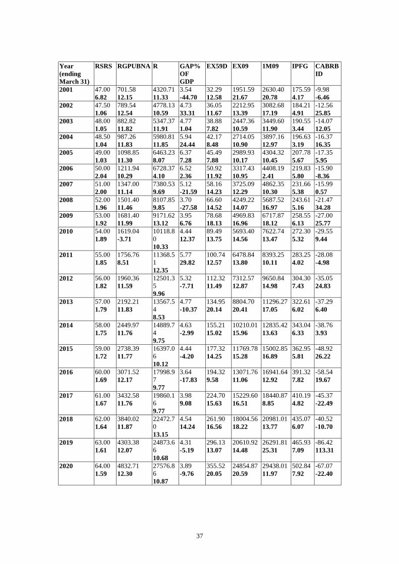
Year(ending March 31)
RSUS RGPUBNA
R GAP %OFGDP
EX59D EX09 IM09 IPFG CABRBID
47.006.82
714.5013.17
4442.9812.79
2.88-51.41
32.2912.58
1951.5921.67
2747.7223.03
175.914.26
-11.954.48
47.501.06
821.0413.65
4970.8311.88
3.8433.01
36.0511.67
2212.9513.39
3281.3619.42
184.775.03
-16.1435.07
48.001.05
917.4612.98
5623.8413.14
3.994.04
38.887.82
2447.3610.59
3737.0513.89
191.423.60
-19.3619.92
48.501.04
1036.4012.96
6343.6012.80
5.1428.71
42.178.48
2714.0510.90
4294.7814.92
197.913.39
-23.7222.55
49.001.03
1167.5612.65
6950.869.57
5.466.37
45.497.88
2989.9310.17
4863.0013.23
209.655.93
-27.7016.77
50.002.04
1304.4111.72
7343.465.65
5.36-1.95
50.9211.92
3317.4310.95
5169.616.31
222.456.10
-30.7410.96
51.002.00
1468.7912.60
8155.8911.06
4.02-25.01
58.1614.23
3725.0912.29
5367.933.84
235.215.74
-24.64-19.84
52.001.96
1657.3612.84
9068.5811.19
2.80-30.35
66.6014.52
4249.2214.07
6270.6716.82
248.345.58
-31.1526.42
53.001.92
1877.3313.27
10352.6514.16
3.2817.32
78.6818.13
4969.8316.96
7621.2521.54
264.736.60
-42.6236.84
54.001.89
1834.91-2.26
11590.7311.96
3.8216.38
89.4913.75
5693.4014.56
8763.8014.99
280.305.88
-49.0915.18
55.001.85
2017.899.97
13203.2013.91
5.1434.56
100.7412.57
6478.8413.80
10403.9218.71
293.234.62
-63.9430.25
56.001.82
2279.7812.98
14713.4011.44
4.83-6.05
112.3211.49
7312.5712.87
12249.3917.74
316.698.00
-80.9926.67
57.001.79
2579.9213.17
16193.8310.06
4.38-9.25
134.9520.14
8804.7020.41
14546.9518.76
337.846.68
-94.0816.17
58.001.75
2913.2712.92
17940.7710.79
4.512.96
155.2115.02
10210.0115.96
17327.4819.11
361.577.02
-117.1024.46
59.001.72
3287.9212.86
19929.6611.09
4.540.61
177.3214.25
11769.7815.28
20346.7417.42
385.336.57
-140.6720.13
60.001.69
37.19.8213.14
22095.9210.87
3.89-14.29
194.329.58
13071.7611.06
24676.8221.28
418.278.55
-191.3135.99
61.001.67
4191.4012.68
24528.8711.01
4.3411.39
224.7015.63
15229.6016.51
24249.24-1.73
442.275.74
-139.84-26.90
62.001.64
4725.5312.74
27983.1314.08
5.0616.81
261.9016.56
18004.5618.22
29314.5220.89
473.126.98
-176.6426.32
63.001.61
5334.8313.89
31196.3311.48
4.87-3.89
296.1313.07
20610.9214.48
36067.9223.04
510.917.99
-243.7738.00
64.001.59
6033.3213.09
34891.8411.85
4.59-5.66
355.5220.05
24854.8720.59
45118.3225.09
555.878.80
-321.3431.82

41
Year(ending March 31)
IPFG IM09D EX09D TBDGCSD ZIM09 ZEX09
175.914.26
58.4615.18
41.5213.90
-16.9418.43
858.0019.03
424.8617.93
184.775.03
69.0818.16
46.5912.20
-22.4932.79
994.4215.90
467.9710.15
191.423.60
77.8612.70
50.999.44
-26.8719.45
1103.8811.01
503.497.59
197.913.39
88.5513.74
55.969.75
-32.5921.30
1235.2511.90
543.187.88
209.655.93
99.2412.07
61.029.04
-38.2317.28
1363.8810.41
582.057.16
222.456.10
103.394.18
66.358.73
-37.04-3.09
1424.864.47
623.717.16
235.215.74
105.251.80
73.0410.09
-32.21-13.04
1460.762.52
675.308.27
248.345.58
120.5914.57
81.7211.88
-38.8720.68
1662.9113.84
744.6710.27
264.736.60
143.8019.24
93.7714.75
-50.0328.69
1961.5017.96
841.2212.97
280.305.88
162.2912.86
105.4312.44
-56.8613.66
2206.9212.51
933.6810.99
293.234.62
189.1616.56
117.8011.73
-71.3725.51
2553.8015.72
1030.1410.33
316.698.00
218.7415.64
130.5810.85
-88.1623.53
2937.1515.01
1127.649.46
337.846.68
255.2116.67
154.4718.29
-100.7414.27
3405.1215.93
1315.1916.63
361.577.02
298.7517.06
176.0313.96
-122.7221.81
3958.9616.26
1478.5312.42
385.336.57
344.8615.43
199.4913.32
-145.3718.46
4549.7714.92
1652.6311.77
418.278.55
411.2819.26
217.869.21
-193.4233.05
5377.1318.18
1780.767.75
442.275.74
397.53-3.34
249.6714.60
-147.86-23.55
5348.98-0.52
2011.5412.96
473.126.98
472.8118.94
290.4016.31
-182.4223.37
6312.6518.02
2309.3314.80
510.917.99
572.5121.08
327.1612.66
-245.3534.50
7560.2419.76
2565.5811.10
555.878.80
704.9723.14
388.3618.71
-316.6229.05
9181.8721.45
2998.8616.89
42
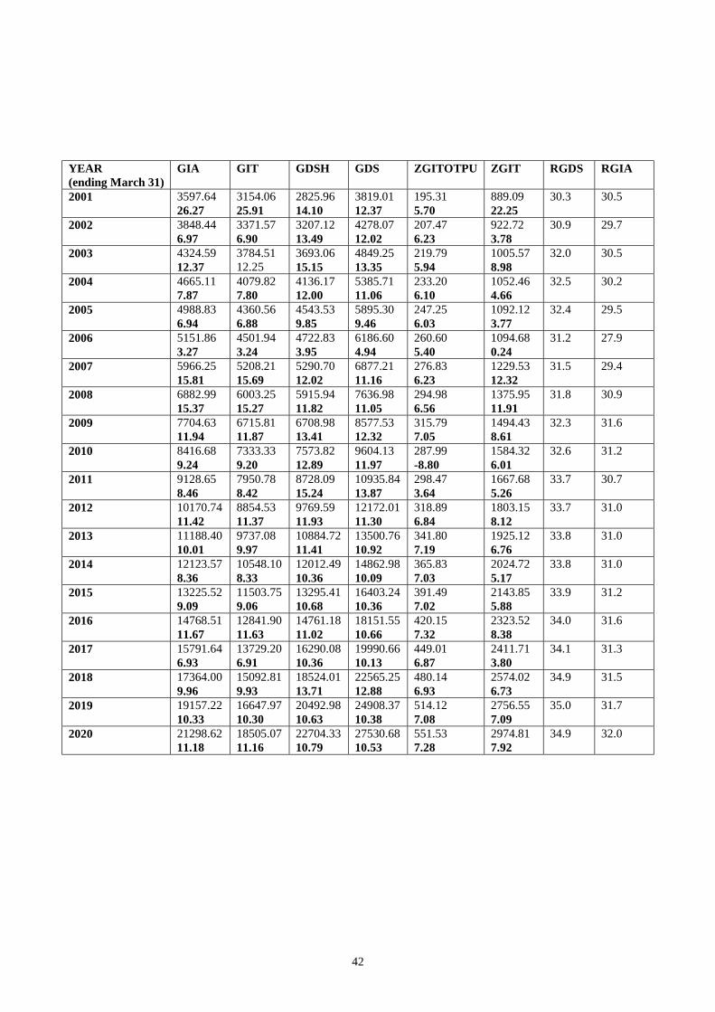
YEAR(ending March 31)
GIA GIT GDSH GDS ZGITOTPU ZGIT RGDS RGIA
2001 3597.6426.27
3154.0625.91
2825.9614.10
3819.0112.37
195.315.70
889.0922.25
30.3 30.5
2002 3848.446.97
3371.576.90
3207.1213.49
4278.0712.02
207.476.23
922.723.78
30.9 29.7
2003 4324.5912.37
3784.5112.25
3693.0615.15
4849.2513.35
219.795.94
1005.578.98
32.0 30.5
2004 4665.117.87
4079.827.80
4136.1712.00
5385.7111.06
233.206.10
1052.464.66
32.5 30.2
2005 4988.836.94
4360.566.88
4543.539.85
5895.309.46
247.256.03
1092.123.77
32.4 29.5
2006 5151.863.27
4501.943.24
4722.833.95
6186.604.94
260.605.40
1094.680.24
31.2 27.9
2007 5966.2515.81
5208.2115.69
5290.7012.02
6877.2111.16
276.836.23
1229.5312.32
31.5 29.4
2008 6882.9915.37
6003.2515.27
5915.9411.82
7636.9811.05
294.986.56
1375.9511.91
31.8 30.9
2009 7704.6311.94
6715.8111.87
6708.9813.41
8577.5312.32
315.797.05
1494.438.61
32.3 31.6
2010 8416.689.24
7333.339.20
7573.8212.89
9604.1311.97
287.99-8.80
1584.326.01
32.6 31.2
2011 9128.658.46
7950.788.42
8728.0915.24
10935.8413.87
298.473.64
1667.685.26
33.7 30.7
2012 10170.7411.42
8854.5311.37
9769.5911.93
12172.0111.30
318.896.84
1803.158.12
33.7 31.0
2013 11188.4010.01
9737.089.97
10884.7211.41
13500.7610.92
341.807.19
1925.126.76
33.8 31.0
2014 12123.578.36
10548.108.33
12012.4910.36
14862.9810.09
365.837.03
2024.725.17
33.8 31.0
2015 13225.529.09
11503.759.06
13295.4110.68
16403.2410.36
391.497.02
2143.855.88
33.9 31.2
2016 14768.5111.67
12841.9011.63
14761.1811.02
18151.5510.66
420.157.32
2323.528.38
34.0 31.6
2017 15791.646.93
13729.206.91
16290.0810.36
19990.6610.13
449.016.87
2411.713.80
34.1 31.3
2018 17364.009.96
15092.819.93
18524.0113.71
22565.2512.88
480.146.93
2574.026.73
34.9 31.5
2019 19157.2210.33
16647.9710.30
20492.9810.63
24908.3710.38
514.127.08
2756.557.09
35.0 31.7
2020 21298.6211.18
18505.0711.16
22704.3310.79
27530.6810.53
551.537.28
2974.817.92
34.9 32.0

43
Year(ending March 31)
RSUS RGPUBNA R GAP%OFGDP
EX59D EX09 1M09 IPFG CABRBID
2001 47.006.82
485.1013.15
4289.0211.58
5.50-35.87
32.2912.58
1951.5921.67
2529.2321.72
171.433.30
-7.09-5.89
2002 47.501.06
550.9913.58
4760.1110.98
6.6320.63
36.0511.67
2212.9513.39
2973.5317.57
178.294.00
-9.5234.29
2003 48.001.05
621.0312.71
5343.3312.25
6.802.56
38.887.82
2447.3610.59
3321.8411.71
182.662.45
-10.6311.65
2004 48.501.04
699.4412.63
5988.8212.08
8.0919.02
42.178.48
2714.0510.90
3741.0212.62
186.522.12
-12.3215.94
2005 49.001.03
784.8612.21
6511.458.73
8.545.44
45.497.88
2989.9310.17
4139.8910.66
195.204.65
-13.116.42
2006 50.002.04
871.6611.06
6819.284.73
8.621.04
50.9211.92
3317.4310.95
4242.902.49
204.474.75
-11.48-12.41
2007 51.002.00
976.4212.02
7526.4210.37
7.37-14.57
58.1614.23
3725.0912.29
4679.9210.30
213.234.28
-11.18-2.62
2008 52.001.96
1095.9512.24
8302.7210.31
6.11-17.10
66.6014.52
4249.2214.07
5467.7616.83
221.804.02
-15.8541.73
2009 53.001.92
1235.1012.70
9418.8113.44
6.699.49
78.6818.13
4969.8316.96
6411.4717.26
232.945.02
-19.5623.41
2010 54.001.89
1131.84-8.36
10464.9411.11
7.238.16
89.4913.75
5693.4014.56
7271.9513.42
242.584.13
-21.168.19
2011 55.001.85
1223.658.11
11816.1912.91
8.6319.33
100.7412.57
6478.8413.80
7978.509.72
249.042.67
-18.38-13.16
2012 56.001.82
1374.2012.30
13071.9010.63
8.42-2.46
112.3211.49
7312.5712.87
9123.2914.35
264.926.38
-23.0825.60
2013 57.001.79
1546.7912.56
14249.189.01
8.05-4.40
134.9520.14
8804.7020.41
10607.9716.27
277.604.79
-22.21-3.79
2014 58.001.75
1735.1212.18
15627.939.68
8.374.00
155.2115.02
10210.0115.96
11758.5410.85
291.725.08
-16.38-26.22
2015 59.001.72
1943.2612.00
17184.739.96
8.592.60
177.3214.25
11769.7815.28
13392.3113.89
302.704.45
-19.3818.31
2016 60.001.69
2180.9712.23
18829.579.57
7.97-7.18
194.329.58
13071.7611.06
14691.819.70
325.186.72
-22.3815.48
2017 61.001.67
2432.6711.55
20683.219.84
8.749.62
224.7015.63
15229.6016.51
15174.313.28
335.603.20
-25.3813.40
2018 62.001.64
2712.5611.51
23272.3412.52
9.599.75
261.9016.56
18004.5618.22
16444.158.37
350.954.57
-28.3811.82
2019 63.001.61
3026.5211.57
25629.9910.13
9.53-0.59
296.1313.07
20610.9214.48
20172.3022.67
371.055.73
-31.3810.57
2020 64.001.59
3381.1211.72
28266.8310.29
9.29-2.50
355.5220.05
24854.8720.59
21268.435.43
395.816.67
-34.389.56

44
Year(ending March 31)
IPFG IM09D EX09D TBDGCSD ZIM09 ZEX09
171.433.30
53.8113.95
41.5213.90
-12.2914.10
793.6717.70
424.8617.93
178.294.00
62.6016.33
46.5912.20
-16.0130.28
905.4614.09
467.9710.15
182.662.45
69.2010.55
50.999.44
-18.2213.78
986.148.91
503.497.59
186.522.12
77.1311.46
55.969.75
-21.1716.23
1081.479.67
543.187.88
195.204.65
84.499.53
61.029.04
-23.4710.83
1167.367.94
582.057.16
204.474.75
84.860.44
66.358.73
-18.51-21.13
1178.300.94
623.717.16
213.234.28
91.768.14
73.0410.09
-18.721.15
1270.757.85
675.308.27
221.804.02
105.1514.59
81.7211.88
-23.4325.16
1442.2713.50
744.6710.27
232.945.02
120.9715.05
93.7714.75
-27.2016.08
1643.5913.96
841.2212.97
242.584.13
134.6711.32
105.4312.44
-29.237.47
1820.8610.79
933.6810.99
249.042.67
145.067.72
117.8011.73
-27.27-6.72
1961.207.71
1030.1410.33
264.926.38
162.9212.31
130.5810.85
-32.3318.59
2191.9411.77
1127.649.46
277.604.79
186.1014.23
154.4718.29
-31.64-2.16
2486.4113.43
1315.1916.63
291.725.08
202.738.94
176.0313.96
-26.70-15.61
2709.308.96
1478.5312.42
304.704.45
226.9911.96
199.4913.32
-27.503.00
3022.4311.56
1652.6311.77
325.186.72
244.867.87
217.869.21
-27.00-1.82
3272.398.27
1780.767.75
335.603.20
248.761.59
249.6714.60
0.91-103.36
3379.383.27
2011.5412.96
350.954.57
265.236.62
290.4016.31
25.172676.67
3635.867.59
2309.3314.80
371.055.73
320.2020.72
327.1612.66
6.96-72.34
4313.2018.63
2565.5811.10
395.816.67
332.323.79
388.3618.71
56.04704.89
4555.805.62
2998.8616.89