Embed Size (px)
Citation preview
University of Texas at El PasoDigitalCommons@UTEP
Open Access Theses & Dissertations
2012-01-01
Sustainable Disposal Of BrineBijoy Krishna HalderUniversity of Texas at El Paso, [email protected]
Follow this and additional works at: https://digitalcommons.utep.edu/open_etdPart of the Biology Commons, and the Civil Engineering Commons
This is brought to you for free and open access by DigitalCommons@UTEP. It has been accepted for inclusion in Open Access Theses & Dissertationsby an authorized administrator of DigitalCommons@UTEP. For more information, please contact [email protected].
Recommended CitationHalder, Bijoy Krishna, "Sustainable Disposal Of Brine" (2012). Open Access Theses & Dissertations. 2101.https://digitalcommons.utep.edu/open_etd/2101

SUSTAINABLE DISPOSAL OF BRINE
BIJOY KRISHNA HALDER
Department of Civil Engineering
APPROVED:
Vivek Tandon, Ph.D., Chair
Ramana V. Chintalapalle, Ph.D., Co-Chair
Siddhartha Das, Ph.D.
Anthony Tarquin, Ph.D.
Benjamin C. Flores, Ph.D.
Interim Dean of the Graduate School

Copyright ©
by
Bijoy K. Halder
2012

Dedication
Dedicated to my parent for all their support
SUSTAINABLE DISPOSAL OF BRINE
by
BIJOY KRISHNA HALDER
THESIS
Presented to the Faculty of the Graduate School of
The University of Texas at El Paso
in Partial Fulfillment
of the Requirements
for the Degree of
MASTER OF SCIENCE
Department of Civil Engineering
THE UNIVERSITY OF TEXAS AT EL PASO
August 2012

v
Acknowledgements
I would like to start by expressing my gratitude to my advisor committee chairman
Professor Vivek Tandon for giving me the opportunity to work in this multidisciplinary research
project. His supports are the reason I was able to accomplish this work. Also my special thanks
to Professor Chintalapalle Ramanna, Professor Siddhatha Das and Professor Anthony Tarquin
for serving on my defense committee. In addition, I need to thank Professor Shane Walker too
for his advice.
I would like to gratefully acknowledge financial support for this project received from the
Center of Inland Desalination Systems and Civil Engineering Department, UTEP. This project
was conducted in different lab of Biomolecule Analysis Core Facility, Center for Transportation
Infrastructure Systems, Center of Inland Desalination Systems and Nano Material Integration
Lab at University of Texas at El Paso. I would also like to acknowledge the assistance of
Chandan Roy, Neo Ortega, Jose Garibey, and David Powell for support in performance and
preparation of experimental design.
In addition, I must acknowledge for that advice, assistance, guidance and encourage to
Debarshi Roy (PhD) of Microbiology Department, UTEP.
I would finally like to express my deepest appreciation and gratitude to my family. I
would like to thanks my parents for their love and support through path of self-discovery and my
friends for staying in touch despite the distance.

vi
Abstract
To meet growing water demand, more water is being harvested from nontraditional
sources like brackish water from deep underground aquifers. Since these sources contain salts,
drinkable water is produced by separating salt and other minerals (TDS, Total Dissolved Solids)
from water through a process commonly known as desalination. A typical desalination plant
produces 50-60% potable water from brackish water and the remaining water (brine) is disposed
in evaporation ponds or by injecting it below the ground surface. To maximize the limited water
supply, inland desalination plants have developed technologies to reduce brine production
commonly known as zero liquid discharge (ZLD) technology. Although the technology allows
maximum water recovery, the produced brine consists of very high TDS (more than 10,000 mg
per liter of water) which makes current disposal practices unsustainable. The disposal of such a
large quantity of salt in an economical and sustainable environmental friendly manner can only
be achieved by using it as a construction material and was the main focus of this research. In this
study, it is proposed to use TDS in place of sand to prepare mortar for application in highway
infrastructure like vertical moisture barrier or embankment fill material. However, addition of
TDS (mainly highly concentrated sodium chloride) weakens the integrity of cement matrix, thus,
resulting in lower strength and durability of mortar. To improve durability and reduce leaching
of TDS, fly ash and aerobic bacteria were used. The use of fly ash increases the long term
strength and durability while reducing required cement content. Any reduction in cement content
translates into reduction in carbon footprint because fly ash is a byproduct. In addition, fly ash
creates optimum environment for bacterial growth by lowering pH of mortar matrix.
The aerobic bacteria were also used to increase compressive strength and stabilize salt by
calcite precipitation and by minimizing porosity. Since addition of salt increases pH of the
mortar environment, the survivability of bacteria becomes an issue. To survive in high pH
(around 12) mortar environment, the bacteria were mutated by exposing them to ultraviolet rays.
The advantage of mutation is that the bacteria can withstand higher pH as well as helps in

vii
formation of more calcite than normal bacteria. The use of mutated bacteria in association with
fly ash not only creates finer pores for bacterial growth, but also lowers the pH of mortar matrix
by consuming free lime or calcium hydroxide, formed during hydration of cement.
The mutated bacteria, fly ash and salt/TDS were used to prepare mortar specimens. These
specimens were subjected to strength and durability tests (such as freeze thaw test, water
permeability test and absorption test). In addition to strength and durability tests, micro-level
analysis of mortar was performed using X-ray diffraction and scanning electron microscopy
techniques. This type of experiments provided the crystallography and mineral information to
explain the behavior of samples from micro-scale point of view.
The test results indicated that fly ash and microorganism application not only improves
the strength and durability, but also stabilized TDS by sealing or reducing the void space of
specimens.

viii
Table of Contents
Acknowledgements ......................................................................................................... v
Abstract .......................................................................................................................... vi
Table of Contents ......................................................................................................... viii
List of Tables ................................................................................................................. xii
List of Figures .............................................................................................................. xiii
Chapter 1: Introduction ...................................................................................................... 1
1.1 Problem Statement ................................................................................................ 1
1.2 Objective & Scope ................................................................................................ 3
1.3 Organization .......................................................................................................... 4
Chapter 2: Literature Review ............................................................................................ 6
2.1 Desalination ............................................................................................................... 6
2.1.1 Introduction ........................................................................................................ 6
2.1.2 Desalination Technique ...................................................................................... 7
2.1.2 Environmental Impact of Desalination ............................................................. 11
2.1.3 Summary ........................................................................................................... 13
2.2 Fly Ash .................................................................................................................... 15
2.2.1 Introduction ...................................................................................................... 15
2.2.2 Chemical Composition ..................................................................................... 17
2.2.3 Crystalline Composition ................................................................................... 20
2.2.4 Glassy Composition .......................................................................................... 23

ix
2.2.5 Physical Properties ........................................................................................... 24
2.2.6 Pozzolanic Activity of Fly Ash in Concrete/ Mortar ........................................ 26
2.2.7 Influence of Fly Ash on Hardened PCC ........................................................... 28
2.2.8 Summary ........................................................................................................... 31
2.3 Biocementation ........................................................................................................ 31
2.3.1 Introduction ...................................................................................................... 31
2.3.2 Bacteria ............................................................................................................. 32
2.3.3 Microbiologically Induced Carbonate Precipitation (MICP) ........................... 34
2.3.4 Biocementation in Concrete ............................................................................. 38
2.3.5 Conclusion ........................................................................................................ 39
Chapter 3: Experiment Design and Evaluation Tests ...................................................... 41
3.1 Experiment Design .................................................................................................. 41
3.2 Culture of Bacteria .................................................................................................. 44
3.2.1 Introduction ...................................................................................................... 44
3.2.2 Constituents Required for Bacteria Growth ..................................................... 44
3.3 Mortar Ingredients and Properties ........................................................................... 48
3.2.2 Mix Proportion and Specimen Preparation ...................................................... 51
3.3 Compressive Strength Test ...................................................................................... 54
3.4 Durability Tests ....................................................................................................... 55
3.4.1 Freeze Thaw Test.............................................................................................. 55
3.4.2 Water Permeability Test ................................................................................... 57
3.4.3 Absorption or Sorptivity Test ........................................................................... 59

x
3.5 Micro Level Tests .................................................................................................... 63
3.5.1 XRD Analysis ................................................................................................... 63
3.5.2 Scanning Electron Microscopy ......................................................................... 65
Chapter 4: Results & Discussions ................................................................................... 67
4.1 Bacteria Growth ...................................................................................................... 67
4.2 Salt (Brine) .............................................................................................................. 70
4.2.1 XRD Analysis ................................................................................................... 71
4.2.2 SEM Analysis ................................................................................................... 71
4.3 Fly Ash .................................................................................................................... 75
4.3.1 XRD Analysis ................................................................................................... 75
4.3.2 SEM Analysis ................................................................................................... 77
4.3.3 EDS Analysis .................................................................................................... 79
4.4 Mortar ...................................................................................................................... 81
4.4.1 Compressive Strength Test ............................................................................... 81
4.4.2 Freeze Thaw Test.............................................................................................. 88
4.4.3 Water Permeability Test ................................................................................... 90
4.4.4 Absorption Test ................................................................................................ 93
4.4.5 XRD Analysis ................................................................................................. 104
4.4.6 SEM Analysis ................................................................................................. 106
Chapter 5: Summary and Conclusions .......................................................................... 113
5.1 Suggestions for Future Research ........................................................................... 115
References ................................................................................................................... 117

xi
Appendix A ................................................................................................................. 126
Appendix B ................................................................................................................. 149
Vita .............................................................................................................................. 153

xii
List of Tables
Table 2.1: Bulk Composition Of Fly Ash With Coal
Sources [Source: ( ACI Committee 232, 1996)] ................................................................... 18
Table 2.2: Mineralogical Phases In Fly Ash [Source: ( ACI Committee 232, 1996)] .................. 21
Table 3.1: Specimen Size And Tests Performed .......................................................................... 42
Table 3.2: Amount Of Mortar Components .................................................................................. 43
Table 3.3: Ingredients Of Tris-Ye Bacteria Culture Medium ....................................................... 45
Table 3.4: Main Constituents In A Typical Portland Cement
(Adapted From Mindess And Young, 1981) ........................................................................ 49
Table 3.5: Sieve Analysis Of Fine Aggregate .............................................................................. 50
Table 3.6: Analytical Report Of Brackish Water Is Used
In El Paso Inland Desalination Plant [Source: (Tarquin, 2010)]……………………….. .... 52
Table 3.7: Composition Of Urea Calcium Chloride Medium ....................................................... 53
Table 4.1: Optical Density (OD600) Of Bacteria Samples ............................................................. 68
Table 4.2: Elemental Composition Of Salt ................................................................................... 74
Table 4.3: Elemental Composition Of Fly Ash ............................................................................ 80
Table 4.4: Comparison Between CSFP5%, CSSFP5%,
CSFMB5% And CSSFMB5% .............................................................................................. 87
Table 4.5: Output Of Water Permeability Test ............................................................................. 91
Table 4.6 : Amount Of Chlorine Leached From Salt Used
In CSFMB 5% Sample........................................................................................................ 101
Table 4.7: Elemental Analysis Result Of Different Samples ..................................................... 110

xiii
List of Figures
Figure 1.1: Total Water Withdrawal By Region, 1995 And 2025
(Mark et al., 2002) .................................................................................................................. 1
Figure 2.1: Worldwide Cumulative Capacity Of Desalination
Plants [Source: (Desalination, 2008)] ..................................................................................... 7
Figure 2.2: Desalination Process [Source: (Tsiourtis X., 2001)] .................................................... 8
Figure 2.3: Schematic Of Reverse Osmosis Process
[Source: (Thomson, 2003)] ................................................................................................... 10
Figure 2.4: Fly Ash Lifecycle [Source: (Will, November 2011)] ................................................. 16
Figure 2.5: Fly Ash Reaction With Cement [Source: (King, 2005)] ............................................ 17
Figure 2.6: Typical Fly Ash Mineralogy
[Source: (Portland Concrete Association)] ........................................................................... 20
Figure 2.7: Cao-SiO2-Al2O3 Ternary System Diagram
[Source: ( ACI Committee 232, 1996)] ................................................................................ 24
Figure 2.8: Fly Ash Showing Solid Sphere At 4000 Magnification
[Source: ( ACI Committee 232, 1996)] ................................................................................ 25
Figure 2.9: Fly Ash Showing Pleroshere At 2000 Magnification
[Source: ( ACI Committee 232, 1996)] ................................................................................ 25
Figure 2.10: The Bacterial Growth (Friedrich, 2010) ................................................................... 33
Figure 3.1: Cell Culture Hood (Labgard, Class-Ii, Type A2) ....................................................... 46
Figure 3.2: Shake Incubator .......................................................................................................... 46
Figure 3.3: Spectrophotometer ...................................................................................................... 47
Figure 3.4: Germicidal Lamp ........................................................................................................ 48
Figure 3.5: Typical Oxide Composition Of A General-Purpose
Portland Cement (Adapted From Mindess And Young, 1981) ............................................ 49
Figure 3.6: A Universal Compressive Testing Machine ............................................................... 54

xiv
Figure 3.7: Environmental Chamber............................................................................................. 56
Figure 3.8: Schematic Diagram Of Test Configuration ................................................................ 58
Figure 3.9: Experimental Setup Of Water Permeability Test ....................................................... 58
Figure 3.10: Schematic Of The Testing Procedure ....................................................................... 60
Figure 3.11: Ion Chromatography System .................................................................................... 62
Figure 3.12: Ion Analysis Process (Dionex ICS-2100 Ion
Chromatography System Operator) ...................................................................................... 62
Figure 3.13: Bruker D8 X-Ray Diffractometer ............................................................................. 64
Figure 3.14: Schematic Of X-Ray Diffraction .............................................................................. 65
Figure 3.15: Hitachi S-4800 Scanning Electron Microscope ....................................................... 66
Figure 3.16: Schematic Of Scanning Electron Microscope .......................................................... 66
Figure 4.1: Bacteria Growth Curve ............................................................................................... 69
Figure 4.2: XED Pattern Of Salt Particle ...................................................................................... 72
Figure 4.3: SEM Image Of Salt .................................................................................................... 73
Figure 4.4: EDS Spectra Of Salt Particle ...................................................................................... 74
Figure 4.5: X-Ray Diffraction Pattern For Fly Ash ...................................................................... 76
Figure 4.6: SEM Images Of Fly Ash Samples .............................................................................. 78
Figure 4.7: The Particle Size Distribution Of Fly Ash ................................................................. 79
Figure 4.8: EDS Spectra Of Fly Ash ............................................................................................ 80
Figure 4.9: Strength Of Different Type Of Mortar Specimens ..................................................... 83
Figure 4.10: Strength Activity Index Of Mortar Specimens......................................................... 84
Figure 4.11: Strength Growth Rate Of Mortar Specimens .......................................................... 85
Figure 4.12: Freeze Thaw Test Result .......................................................................................... 89
Figure 4.13: Intrinsic Permeability (m2) Of Specimens................................................................ 92
Figure 4.14: Initial Absorption Rate Of Different Samples .......................................................... 94
xv
Figure 4.15: Predicted Water Absorption To Sample Mass
Ratio With Respect To Time ................................................................................................ 96
Figure 4.16: Amount Of Sodium (Mg/G) Leached From
Samples After 8 Days Of Absorption ................................................................................... 98
Figure 4.17: Amount Of Chlorine (Mg/G) Leached From
Samples After 8 Days Of Absorption ................................................................................... 99
Figure 4.18: Amount Of Calcium (Mg/G) Leached From
Samples After 8 Days Of Absorption ................................................................................. 100
Figure 4.19: Ph After 8 Days Of Absorption Testing ................................................................. 103
Figure 4.20:X-Ray Diffraction Pattern For Different Samples
In 3-D Scale ........................................................................................................................ 104
Figure 4.21: X-Ray Diffraction Pattern Of Samples
From 20º To 40
º ................................................................................................................... 105
Figure 4.22: SEM Image At 2000 Magnification Of
Different Samples ............................................................................................................... 107
Figure 4.23: SEM Image At 8000 Magnification Of
Different Samples ............................................................................................................... 108
Figure 4.24: SEM Image With Bacteria And Crystal Size ......................................................... 109
Figure 4.25: EDS Spectrum Analysis Of Different Samples ...................................................... 111

1
Chapter 1: Introduction
1.1 Problem Statement
Water is the critical resource for well-being of humans and the environment. With the
increase in human populations, the demand (whether for direct consumption or indirectly needed
for agriculture) for water supply has increased exponentially. According to Mark et al. (2002),
water demand is expected to increase from 4,000 cubic kilometers ( BGD) to 5,000 cubic
kilometers ( BGD), an increase of 25% from 1995 to 2025, as shown in Figure 1.1.
Figure 1. 1: Total Water Withdrawal by Region, 1995 and 2025 (Mark et al., 2002)
Finite fresh water resources are coming under increasing pressure from population
growth and over use. To meet this growing water demand, more water is being harvested from
nontraditional sources like seawater or brackish water from deep underground aquifers. Since
both of the sources contain dissolved solids (mainly salts and other minerals), drinkable water is
produced by separating total dissolved solids (TDS) from water through a process commonly

2
known as desalination. During the desalination process, the saline water is passed through
membranes/nano-filters/electro-dialysis to obtain potable water, with Total Dissolved Solids
(TDS) less than 500 mg/liter (Desalination, 2008). However, this process also produces a
byproduct commonly known as brine (Mickley, 2006) which consists of higher amounts of TDS
(more than 7,500 mg/liter of water).
A typical desalination plant produces 35-50% potable water from sea water and 50-90%
from brackish water (Desalination, 2008). This desalination technique is acceptable near oceans
because brine is discharged back to the sea. Although this process may harm sea creatures and
plants, this is an acceptable practice for now. However, the same disposal choice is not available
for inland desalination plants because it is far from the sea and there is only a limited supply of
brackish water. To maximize the limited water supply, inland desalination plants have developed
technologies to reduce brine production commonly known as zero liquid discharge (ZLD)
technology. Although the technology allows maximum water recovery, the produced brine
consists of very high TDS (more than 10,000 mg per liter of water). Since concentrated brine has
a high concentration of TDS or salts, TDS which is highly corrosive due to the presence of
concentrated sodium, chloride, phosphate, nitrates ions etc, an improper discharge can be
detrimental to the environment in which it is disposed. To mitigate environmental damage, the
current disposal practices include but are not limited to: evaporation ponds (with proper lining)
and injection below the ground surface.
Although currently practiced, these disposal techniques are not sustainable because the
presence of salts in a high concentration will lead to soil salinity. Moreover, these options are not
always available when the desalination plant is close to urban populations. The disposal of such a
large quantity of salt in an economical and sustainable environmentally friendly manner can be
achieved by using it as a construction material, and that is the main focus of this research.
To identify the feasibility of using salt as a construction material, a comprehensive
literature review was conducted. Based on the literature review and field experience, it was
concluded that salt obtained from a desalination plant can be used in place of sand commonly
3
used in construction. Since salt is water soluble, the salt needs to be stabilized before it can be
used as a construction material. In addition, use of salt in place of sand may not be suitable in
Portland cement concrete (PCC) because of higher performance requirements. Therefore, the
most logical place to dispose of salt can be mortar (consisting of salt, sand, water, and cement)
which can be used in highway infrastructure such as vertical moisture barriers or embankment
fills.
Although cement is glue which holds sand particles together, the presence of salt will
reduce the strength and durability of mortar. According to Berke et al. (1988), highly
concentrated sodium chloride or TDS may weaken the integrity of the cement matrix when
mixed with cement sand in mortar. Furthermore, mortar exposed to climate can come in contact
with water and may leach the sodium chloride and other corrosive materials that might be an
environmental concern. To compensate for the loss of durability and strength, fly ash (a coal by
product) was added in the mix (ACI Committee 232, 1996). Fly ash, in the presence of cement
and water, increases the durability as well as strength. Therefore, the addition of fly ash requires
less cement to obtain similar strength levels. This will reduce the cost of mortar (fly ash is
cheaper than cement) and will minimize the carbon footprint generated due to production of
cement.
In addition to fly ash, mortar consisting of salt was also treated with bacteria to improve
durability. In 2001, Ramchandran et al. found that microorganisms can biologically induce
precipitation of calcite over the surface and pores of mortar, which can improve its strength and
durability. Therefore, cement, sand, fly ash and microorganisms were used to stabilize salt,
thereby maintaining or improving the compressive strength and durability of mortar and is the
objective of this study.
1.2 Objective & Scope
The safe disposal of TDS in a sustainable environmental friendly manner was the main
objective of this research. To achieve this objective, the highly concentrated brine from the plant
4
was gathered and dried to obtain TDS for testing. The solids were then used instead of sand to
produce mortar, a commonly used construction material. The commonly used mortar consists of
sand, cement, and water (Cement: Sand: Water =1.00:2.75:0.485). In this study, it is proposed to
replace a portion of the sand with TDS and determine its influence on the strength of the mortar.
Since TDS mainly consists of concentrated salts such as sodium chloride (NaCl), it can leach out
of the mortar matrix in the presence of water. In addition, the presence of chlorine (Cl) may
weaken the integrity of the cement mortar matrix. Therefore, the long term durability of mortar
consisting of salts was also evaluated in this study.
To achieve objectives of this study, the following tasks were performed:
Physical and chemical properties of brine were evaluated using micro
level testing so that it can be used in mortar or concrete as an alternative of sand.
Compressive strength of mortars was identified using compression testing
equipment.
Influence of microorganisms and fly ash on strength and durability was
evaluated.
Durability tests of mortar were performed to identify long term durability
of mortar.
To validate the influence of fly ash and microorganisms on strength and
durability, micro level tests or nondestructive techniques like scanning electron
microscopy and X-ray diffraction were performed.
1.3 Organization
The thesis is divided into five chapters.
Chapter 1 defines the problem, proposes research objectives and the scope
of this research.
A detailed literature review on desalination, fly ash, bacteria and the
research approach is described in Chapter 2.

5
Chapter 3 includes experiment design and test systems used for
performing macro as well as micro level testing.
In Chapter 4, the results and analysis of test results are included.
Chapter 5 presents the conclusions of this study and recommendations for
future research.
6
Chapter 2: Literature Review
To develop a durable mortar consisting of salt obtained from desalination, it is necessary
to know the physical and chemical properties of salt. Since fly ash and microorganisms will be
added to maintain strength and durability of mortar consisting of salt, an understanding of these
components and their interactions with conventional mortar materials needs to be understood. In
this chapter, a brief discussion on the desalination process and typical salt characteristics
obtained from a local desalination plant is presented. Finally, the relevant literature on fly ash
and microorganisms suitable for conventional mortar is discussed.
2.1 Desalination
2.1.1 Introduction
Water is vital for the very existence of life on earth and a necessity for economic and
social development and for environmental sustainability. Although available in large quantity in
oceans, the availability of water for drinking or for agriculture production is limited, especially
near urban hubs. Since water availability cannot be increased as natural resources of water are
limited, desalination of inland brackish water has become an alternative solution.
The use of water desalination processes is expanding rapidly, especially to support urban
and industrial developments in arid and semi-arid regions and in remote areas where water is
unavailable or it’s too costly to transport. As shown in Figure 2.1, desalination of water has
grown exponentially to meet the growing demand.
According to IDA report No.16, more than 120 countries in all regions produced potable
water from a desalination process (Tsiourtis X., 2001). Since the cost of TDS removal is no
longer a barrier due to advancement of membrane and nano-filtration or electro-dialysis
technology, the use of desalination processes has grown exponentially, which has reduced the
unit production cost from $3-5/m3 in 1980 to $0.5-1.3/m
3 currently (Hisham et al., 2001).

7
Figure 2. 1: Worldwide Cumulative Capacity of Desalination Plants [Source:
(Desalination, 2008)]
2.1.2 Desalination Technique
Desalination is a process that separates TDS from sea or brackish water. The byproduct
of desalination process is reject brine (water with a high concentration of TDS). A significant
amount of energy (6.5-28 kWh m-3
) is typically required, depending on the desalination process,
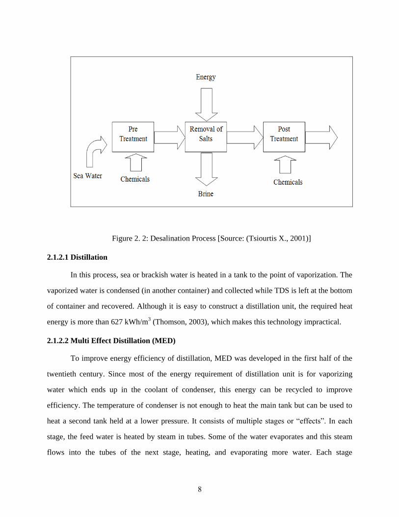
to achieve the desired TDS levels in potable water (DESWARE, 2012). A flow diagram
depicting the desalination process is shown in Figure 2.2.
8
Figure 2. 2: Desalination Process [Source: (Tsiourtis X., 2001)]
2.1.2.1 Distillation
In this process, sea or brackish water is heated in a tank to the point of vaporization. The
vaporized water is condensed (in another container) and collected while TDS is left at the bottom
of container and recovered. Although it is easy to construct a distillation unit, the required heat
energy is more than 627 kWh/m3 (Thomson, 2003), which makes this technology impractical.
2.1.2.2 Multi Effect Distillation (MED)
To improve energy efficiency of distillation, MED was developed in the first half of the
twentieth century. Since most of the energy requirement of distillation unit is for vaporizing
water which ends up in the coolant of condenser, this energy can be recycled to improve
efficiency. The temperature of condenser is not enough to heat the main tank but can be used to
heat a second tank held at a lower pressure. It consists of multiple stages or “effects”. In each
stage, the feed water is heated by steam in tubes. Some of the water evaporates and this steam
flows into the tubes of the next stage, heating, and evaporating more water. Each stage
9
essentially reuses the energy from the previous stage. A series of condensation-evaporation
processes produce water with acceptable TDS. Although more efficient than single distillation
tank, this process did not become popular due to buildup of scaling on outside of heating pipes
(Thomson, 2003).
2.1.2.3 Multi Stage Flash (MSF)
To reduce the energy required for heating water, the water is heated under pressure
(preventing vaporization) and transferred to another tank held at a lower pressure (allowing it
vaporize). Since the entering water temperature is higher than the boiling temperature under a
vacuum, a part of it suddenly vaporizes. For this reason, this process is known as flash
distillation. Fresh water is formed by condensation of this water vapor, which is collected at each
stage and passed on from stage to stage in parallel with brine. At each stage, the product water is
cooled and the surplus heat is recovered to preheat the feed water. Since the second tank is well
away from heating pipes, scaling is minimized. Also, MSF is slightly more energy efficient than
MED and became the industry standard after first introduction in 1960 (Thomson, 2003).
2.1.2.4 Vapor Compression
To minimize energy consumption, water vapors produced during the MSF process are
compressed. The temperature of water vapors rises, under compression, and the temperature
increase is used as a heat source for the same tank of water that produced it. This permits heat
recycling in a configuration of one single step or multi effect. This process is characterized by
low energy consumption and low operation cost.
The vapor compression can be achieved via thermal vapor compression (run by steam) or
via mechanical vapor compression (either by diesel engine or electric motor). The process of
thermal vapor compression is popular for medium-scale desalination plants because they are
simple to operate in comparison to MSF.
The benefit of this system is low operating cost compared to multi stage or multi effect
desalination systems; nonetheless, this system’s energy cost and capital cost are high.
10
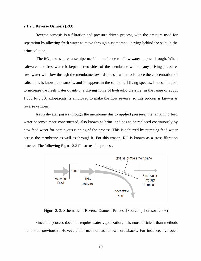
2.1.2.5 Reverse Osmosis (RO)
Reverse osmosis is a filtration and pressure driven process, with the pressure used for
separation by allowing fresh water to move through a membrane, leaving behind the salts in the
brine solution.
The RO process uses a semipermeable membrane to allow water to pass through. When
saltwater and freshwater is kept on two sides of the membrane without any driving pressure,
freshwater will flow through the membrane towards the saltwater to balance the concentration of
salts. This is known as osmosis, and it happens in the cells of all living species. In desalination,
to increase the fresh water quantity, a driving force of hydraulic pressure, in the range of about
1,000 to 8,300 kilopascals, is employed to make the flow reverse, so this process is known as
reverse osmosis.
As freshwater passes through the membrane due to applied pressure, the remaining feed
water becomes more concentrated, also known as brine, and has to be replaced continuously by
new feed water for continuous running of the process. This is achieved by pumping feed water
across the membrane as well as through it. For this reason, RO is known as a cross-filtration
process. The following Figure 2.3 illustrates the process.
Figure 2. 3: Schematic of Reverse Osmosis Process [Source: (Thomson, 2003)]
Since the process does not require water vaporization, it is more efficient than methods
mentioned previously. However, this method has its own drawbacks. For instance, hydrogen
11
sulfide and carbon dioxide and some pesticides or low-molecular-weight organics pass through
the membrane to cause fouling in produced water. Thus, pretreatment is required to remove those
dissolved foul causing matter. At low-cost oxidant (e.g., chlorine) is used for pretreatment;
however, RO membranes cannot tolerate oxidants such as free chlorine, making it essential to
eradicate chlorine from the feedwater before passing it to the RO module. Another drawback is
its relatively low recovery rate in seawater and brackish water desalination (up to about 60 % and
50-90 %, respectively) that yields a large volume of concentrated TDS (Desalination, 2008). The
disposal of concentrated brine water is a major issue, especially for inland desalination plants.
2.1.2.6 Electro-dialysis
Electro-dialysis (ED) is a voltage driven process and uses electrical potential to move
salts selectively through an ion exchange membrane, leaving fresh water behind as potable
water. This method was commercialized during 1960 and it is widely used to desalinate brackish
water. The energy consumption very much depends on the concentration of feed water and for
this reason; electro-dialysis is mainly used for brackish water desalination. Moreover, for the
same reason, this process is mainly used to serve small communities or specific industrial
applications (Thomson, 2003).
2.1.2 Environmental Impact of Desalination
Desalination of water severally impacts the environment as discussed below:
Requirement for increase production of electricity: To produce potable water through the
desalination process, energy, mainly electricity, is needed. Most commonly electrical
energy is produced through burning of fossil fuels, which pollutes the air and causes
global warming (increased carbon footprint).
Brine disposal in sea: After desalination, the reject brine has 1.3 to 1.7 times the original
concentration of seawater. Therefore, reject brine can negatively impact the environment
by disturbing natural sensitivity, which in turn is dependent on the specific nature of the

12
inhabitants and on the specific communities (Einav et al., 2002). An appropriate disposal
system is needed to minimize its impact on the environment.
Impact of cleaning chemicals on marine environment: Brine discharge may contain
different chemicals used in the pretreatment stage of saline water, for example: sodium
hypochlorite (NaOCl), ferric chloride (FeCl3), sulphuric acid (H2SO4) or hydrochloric
acid (HCl), sodium hexametaphosphate, sodium bisulphite (NaHSO3), etc. Also filter
membranes need to be cleaned 3 or 4 times in a year and the chemical products used are
mainly weak acids and detergents (citric acid, sodium polyphosphate and
ethylenediaminetetraacetic acid (EDTA)) and caustic alkali. All of the chemicals used for
pretreatment or cleaning must be neutralized before disposing to the sea.
Impact of noise: RO desalination plants create acoustic pollution. High pressure pumps
and energy recovery systems, such as turbines or similar, produce a significant level of
noise over 90 dB(A).Therefore, they should be located far away from populated areas and
require proper technology to mitigate the influence of noise on employees.
Deep well injection issue: The buried pipes for deep well injection carrying brine for
disposal can leak and salt water can permeate into ground aquifers. Therefore, proper
attention is required to ensure that disposal of brine will not endanger aquifers supplying
drinking water. Also, deep well injection may also cause several large-magnitude
earthquakes. Disposal of brine locally causes increased fluid pressure and vertical
expansion of the aquifer framework, which may be expressed as a rise in the land surface.
Depending on the geologic condition, this increase in fluid pressure can generate
earthquakes (Desalination, 2008).
Adverse effect on soil and ground water: Disposal of brine into unlined ponds or pits
from inland desalination plants has a significant negative environmental impact.
Improper disposal of brine may pollute the groundwater or may change the agricultural
productivity of soil. Higher salt content in reject brine with elevated levels of sodium,
chloride, and boron can reduce plants and soil productivity and increase the risk of soil
13
salinization (Maas et al., 1990). Intrusion of brine in soil induces specific ion toxicity and
changes the sodium absorption ratio (SAR) to alter electrical conductivity. SAR defines
the influence of sodium in soil properties by calculating the relative concentration of
sodium, calcium and magnesium (Mohamed et al., 1998). High SAR values can lead to
lower permeability of soil (Rhoades et al., 1990). Although sodium doesn’t reduce the
intake of water by plants, it changes the soil structure and impairs water infiltration,
affecting plant growth (Hoffman et al., 1990). Other undesirable effects are increased
irrigation requirements and higher rainwater runoff, poor aeration, and reduced leaching
of salts from the root zone because of low permeability. Also, intrusion of heavy metals
and inorganic compounds in groundwater may cause long term health problems.
2.1.3 Summary
Water and the environment are two important factors for sustainability of life on earth.
To meet the growing demand of water from increasing population, desalination is now
imperative. However, development of a viable brine disposal system which is environmentally
friendly and sustainable is still an unusual challenge. Although disposal of reject brine in the
ocean or ponds are commonly used techniques, these methods of disposal are neither sustainable
nor environmentally friendly.
In the previous discussion, it was mentioned that various options exist for the disposal of
reject brine from inland desalination plants. These include waste minimization, discharge to
surface water, and discharge to wastewater treatment plants, deep wells, land application,
evaporation ponds, wastewater evaporators, and irrigation of plants tolerant to high salinity
(halophytes). Mickley et al. (1993) identified the factors that influence the selection of a disposal
method. These include volume or quantity of concentrate, quality or constituents of concentrate,
physical or geographical location of the discharge point of the concentrate, availability of
receiving site, permissibility of the option, public acceptance, capital and operating costs, and
ability for the facility to be expanded.

14
Cost plays an important role in the selection of a brine disposal method. The cost of
disposal depends on the characteristics of the reject brine, the level of treatment before disposal,
means of disposal, volume of brine to be disposed of, and the nature of the disposed
environment. Glueckstern et al. (1996) found that the disposal costs of inland RO desalination
plants are higher than that of plants disposing reject brine in nearby seas or lakes. The disposal of
reject brine must be addressed before the numbers of inland plants increase. Otherwise,
expensive remedial measures will have to be taken to rescue the delicate ecosystems into which
the brine will be disposed or discharged in the future.
Currently, the reject brine produced from El Paso’s inland desalination plant is disposed
of by injecting it more than 2,000 ft. below the ground surface. Other methods of disposal
include use in older oil wells to enhance output, use of reject brine for electricity generation, and
use as a deicing agent. However, these methods are not economically feasible for El Paso
conditions because of cost of transportation. One method of disposal is to allow reject brine to
dry and use the dried salt in cement sand mortar commonly used as a construction material. The
advantage of this disposal method is that a large quantity of salt can be disposed of in an
environmentally friendly manner.
This research will conduct experiments to use brine or salt as an alternative or partial
replacement of aggregate in the construction sector. The main challenge will be to make salt
durable in concrete or mortar without compromising the performance of the concrete or mortar.
The one way it can be stabilized is by reducing or plugging the pores of mortar or concrete.
Recent research on fly ash and microbial activity of calcite deposition found that the strength and
durability of concrete specimens can be improved by using this novel way of calcite precipitation
over the surface and inside pores of samples.
15
2.2 Fly Ash
2.2.1 Introduction
Fly ash is a byproduct of coal combustion and its pozzolanic nature increases strength
and durability of PCC. In a 2008 survey conducted by American Coal Ash Association identified
that 72.4 million tons of fly ash is produced annually of which 42 % is reused while 58% of it is
being disposed in landfill. Since unbounded fly ash is considered hazardous, it is essential to
utilize all of fly ash being produced.
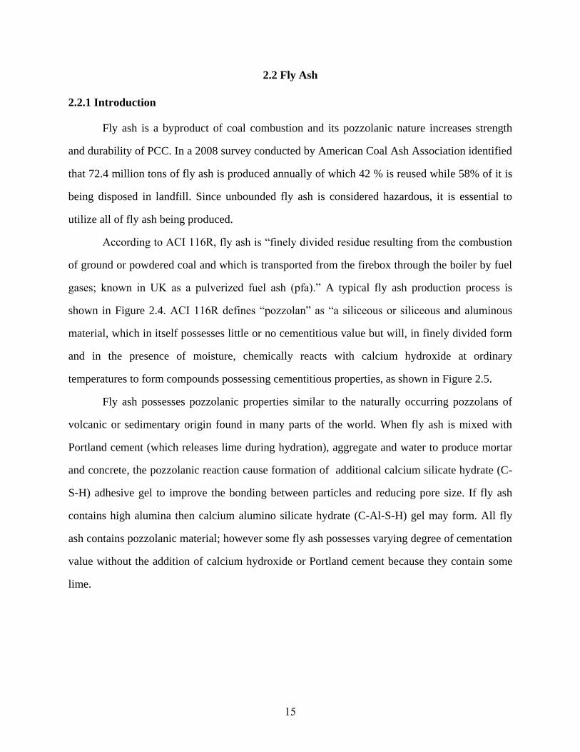
According to ACI 116R, fly ash is “finely divided residue resulting from the combustion
of ground or powdered coal and which is transported from the firebox through the boiler by fuel
gases; known in UK as a pulverized fuel ash (pfa).” A typical fly ash production process is
shown in Figure 2.4. ACI 116R defines “pozzolan” as “a siliceous or siliceous and aluminous
material, which in itself possesses little or no cementitious value but will, in finely divided form
and in the presence of moisture, chemically reacts with calcium hydroxide at ordinary
temperatures to form compounds possessing cementitious properties, as shown in Figure 2.5.
Fly ash possesses pozzolanic properties similar to the naturally occurring pozzolans of
volcanic or sedimentary origin found in many parts of the world. When fly ash is mixed with
Portland cement (which releases lime during hydration), aggregate and water to produce mortar
and concrete, the pozzolanic reaction cause formation of additional calcium silicate hydrate (C-
S-H) adhesive gel to improve the bonding between particles and reducing pore size. If fly ash
contains high alumina then calcium alumino silicate hydrate (C-Al-S-H) gel may form. All fly
ash contains pozzolanic material; however some fly ash possesses varying degree of cementation
value without the addition of calcium hydroxide or Portland cement because they contain some
lime.
16
Figure 2. 4: Fly Ash Lifecycle [Source: (Will, November 2011)]

17
Figure 2. 5: Fly ash reaction with cement [Source: (King, 2005)]
Fly ash is a complex material consisting of heterogeneous combinations of amorphous
(glassy) and crystalline phase. There are two types of glassy spheres, which are solid and hollow
(cenospheres) mostly consist 60 to 90 percent of the total mass of fly ash with the remaining
fraction of fly ash made up of variety of crystalline phase. Actually these two phases are not
separated; rather crystalline phase may exist within a glassy matrix or attached to the surface of
the glassy spheres. This union of phases makes fly ash a complex material to classify and
characterize. Nonetheless, this crystalline phase also affect the compressive strength and
durability of PCC.
Since fly ash is a byproduct, the fly ash obtained from two sources can vary significantly,
it is important to know and understand mineralogical and crystalline phases of fly ash as they
will influence the compressive strength. In the following sections, physical and chemical
properties of fly ash are described.
2.2.2 Chemical Composition
ASTM C618 has classified fly ash into two types, Class C and Class F depending on the
bulk chemical composition. Although classification is based on chemical composition, it doesn’t
address the nature and reactivity of the fly ash particles. The sole purpose of chemical
composition specification is to use it as a quality assurance tool. The crystalline and glassy
18
constituents of fly ash are a result of materials with high melting points and incombustibility.
Although the constituents of fly ash are not typically present as oxides, the chemical composition
of fly ash is reported in terms of oxides.
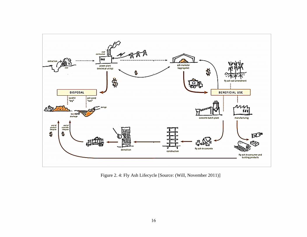
The four main constituents present in fly ash are: SiO2 (35-60%), Al2O3 (10-30%), Fe2O3
(4-20%), CaO (1-35%). For ASTM class F fly ash the sum of first three constituents (SiO2,
Al2O3, Fe2O3) should be greater than 70 %; however, the sum of these constituents should be
greater than 50% to classify fly ash as ASTM Class C. In addition, Class C fly ash has higher
percentage CaO (generally more than 20%) than Class F fly ash. In Table 2.1, the percentages of
constituents present in different source of fly ash available in North America are presented.
The main source of SiO2 in fly ash is clay mineral and quartz. Bituminous coal often
contains a higher percentage of clay minerals in their incombustible fraction than do
subbituminous and lignite coals. Thus, fly ashes obtained from higher rank coal combustion are
richer in silica. This siliceous glass is the primary contributor to form calcium silicate hydrate
(C-S-H) combining with free lime and water during pozzolanic reaction in concrete.
Table 2. 1: Bulk composition of fly ash with coal sources [Source: ( ACI Committee 232,
1996)]
Bituminous Subbituminous Northern
Lignite Southern lignite
SiO2 , % 45.9 31.3 44.6 52.9
Al2O3, % 24.2 22.5 15.5 17.9
Fe2O3,% 4.7 5.0 7.7 9.0
CaO,% 3.7 28.0 20.9 9.6
SO3, % 0.4 2.3 1.5 0.9
MgO,% 0.0 4.3 6.1 1.7
Alkalis,* % 0.2 1.6 0.9 0.6
LOI,* % 3.0 0.3 0.4 0.4
Air
permeability
fineness, m2/kg
403.0 393.0 329.0 256.0
45 µm sieve
retention, % 18.2 17.0 21.6 23.8
Density, Mg/m3 2.28 2.70 2.54 2.43
*LOI is Loss of Ignition; **Available alkalis expressed as Na2O equivalent.
19
Alumina, Al2O3 in fly ash comes mainly from clay in the coal, but some fraction comes
from the organic compounds in low rank coal. The following three groups of clay minerals are
found in coal and source of Al2O3:
Smectite Na(Al5,Mg)Si12O30(OH)6.nH2O
Illite KAl5Si7O20(OH)4
Kaolinite Al4Si4O10(OH)8
The origin of Fe2O3 content in fly ash is due to presence of iron in the coal. The highest
concentration of iron-rich fly ash particle size is in between 30 and 60 µm while particle size less
than 15 µm may also be present.
The amount of CaO in fly ashes depends on the presence of calcium carbonate and
calcium sulfate in coal. High rank coal like bituminous coal contains low noncombustible
materials showing less than 5% of CaO, where for low rank coals it varies from 10-35 percent.
MgO in fly ash actually derived from organic constituents, smectite, ferromagnesian minerals,
and sometimes dolomite. These constituents are typically minimal in high and low rank coal. The
source of SO3 in coal is pyrite (Fe2S) and gypsum (CaSO4.H2O). The sulfur is precipitated onto
the fly ash as sulfur dioxide gas or from the flue gas, through a reaction with lime and alkali
particles.
The presence of alkalis in fly ash is due to clay minerals and other sodium and potassium-
containing constituents. McCarthy et al. (1988) reported that Na2O is found in greater amounts
than K2O in lignite and subbituminous fly ash, but the reverse is true of bituminous fly ash. In
Table 2.1, the alkali contents are expressed as Na2O equivalent (percent Na2O + 0.658 x percent
K2O).
The carbon content in fly ash is a result of incomplete combustion of the coal and organic
additives used in the collection process. It is a measure of loss of ignition (LOI); however LOI
will also include any combined water or CO2, loss due to decomposition of hydrates or
carbonates that may be present in fly ash. The LOI of Class C fly ash is less than 1 percent;
however, LOI of Class F fly ash can be as high as 20 percent. Fly ash used in concrete typically

20
is expected to have less than 6% LOI; however, ASTM C 618 allows up to 12% depending upon
the acceptable performance records and available laboratory test results.
Some minor elements like titanium, phosphorus, lead, chromium and strontium may also
be present in fly ash.
2.2.3 Crystalline Composition
Development of X-ray diffraction (XRD) analysis technique makes it possible to
determine the approximate amounts of crystalline materials in fly ash (McCarthy et al., 1988).
Based on XRD analysis, fly ash can be subdivided in two types: low calcium and high calcium
fly ash. The XRD analysis of low calcium fly ashes identifies presence of relatively inactive
crystalline phases, like quartz, mullite, ferrite spinel, and hematite (Diamond et al., 1981). While
XRD analysis of high calcium fly ash identifies the presence of the four phases plus anhydrite,
alkali sulfate, dicalcium silicate, tricalcium aluminate, lime, melilite, merwinite, periclase, and
sodalite (Gregory J. et al., 1984). A list of crystalline phases found in fly ash is given in Table
2.2 and a pie chart depicting proportion of various fly ash minerals is presented in Figure 2.6.
Figure 2. 6: Typical Fly Ash Mineralogy [Source: (Portland Concrete Association)]
Glassy non crystalline phase that is reactive. Proportion of glass can range from
50-90% of the whole mass.
Inert crystalline
phase

21
Table 2. 2: Mineralogical Phases in Fly Ash [Source: ( ACI Committee 232, 1996)]
Mineral Name Chemical Composition
Thenardite (Na,K)2SO4
Anhydrite CaSO4
Tricalcium Aluminate (C3A) Ca3Al2O6
DiCalcium Silicate (C2S) Ca2SiO4
Hematite Fe2O3
Lime CaO
Melilite Ca2(Mg,Al)(Al,Si)2O7
Merwinite Ca3Mg(SiO2)2
Mullite Al6Si2O3
Periclase MgO
Quartz SiO2
Sodalite Structures
Na8Al8Si6O24SO4
Ca2Na6Al6Si6O24(SO4)2
Ca8Al12O24(SO4)2
Ferrite Spinel Fe3O4
Portlandite Ca(OH)2
Quartz in fly ash is a result of impurities in coal that failed to melt during combustion. In
XRD analysis, quartz is shown as the most intense peak but its amount varies significantly. The
crystalline compound mullite is only found in substantial amount in low calcium fly ash. It is the
main source of alumina in fly ash and forms within the spheres as the glass solidifies around it.
Mullite isn’t chemically active in concrete.
Magnetite (Fe3O4) in its purest form has the crystalline spinel structure in fly ash. A slight
decrease in the diffraction spacing of ferrite spinel is detected through XRD analysis. But this
22
phase is chemically inactive. Hematite (Fe2O3) is formed by the oxidation of magnetite, which is
found in some fly ash and it is too chemically inactive.
Coal ash containing high calcium content often has anhydrite (CaSO4) in the range of 1 to
3 percent. Anhydrite forms due to scrubbing act of the calcium for SO2 in combustion gases.
Crystalline CaO, sometimes referred to as free lime, present in many high calcium fly ash is a
cause of autoclave expansion. On the other hand, if present in the form of slacked lime Ca(OH)2
then it is not responsible for autoclave expansion. Soft-burned CaO hydrates quickly and doesn’t
have any effect on soundness of concrete. But hard-burned CaO, formed at higher temperature to
cause a carbon coated barrier (Demirel et al., 1983) which retards hydration and thereby
decreases the durability. McCarthy et al. (1984) noted that when hard burned lime is present it is
often found in the larger grain of fly ash.
Periclase is crystalline phase of MgO and is found in fly ashes with more than 2% of
MgO. In low rank fly ash, periclase content may go as high as 80% of MgO content. It is not free
MgO typically found in ordinary Portland cement.
Phases belonging to melitite group includes are:
Gehlenite Ca2Al2SiO7
Akarmanite Ca2MgSi2O7
Sodium-Melilite NaCaAlSi2O7
But these phases are not chemically active and Fe may substitute for Al and Mg. Merwinite is a
common phase in high calcium fly ash and forms due to devitrification of Mg-containing glasses.
It is nonreactive at normal temperature.
Diamond (1982) confirmed that tricalcium aluminate C3A is typically present in high
calcium fly ash. In XRD analysis, the peak of this phase overlaps with merwinite and make it
difficult for quantitative analysis. Neither phase is present in low calcium fly ash. The C3A has
self cementitious property and extremely reactive in the presence of calcium and sulfate ions in
solution.

23
Phase related to sodalite group form from melts rich in alkalis, sulfate, calcium and poor
in silica. Among the other phases found in fly ash are alkali sulfate and dicalcium silicate (C2S).
C2S exist in some high calcium fly ashes and as reactive as C2S in Portland cement. Northern
lignite fly ashes often contain crystalline alkali sulfates such as thenardite and aphthitilite.
2.2.4 Glassy Composition
The formation of small glassy sphere in fly ash largely depends on rapid cooling of
burned coal residue. The composition of these glasses varies with composition of the pulverized
coal and the temperature at which it is burned. The major differences in glass composition of fly
ash depend on the amount of calcium present in the glass. All low calcium fly ashes result in
aluminosilicate glassy fly ash particle; however, high calcium fly ash particle form calcium
aluminosilicate fly ash phases (Roy et al., 1984) and is shown in Figure 2.7 (as a ternary system
diagram).
This diagram depicts that glassy composition of high calcium fly ash falls within the
range of anorthite to gelhenite, which are the first phases to crystallize from a melt. In case of
low calcium fly ash, the glass composition plots within mullite region that is the main crystalline
phase. The disorder structure of a glass resembles that of the primary crystalline phase that forms
on cooling from the melt. In fly ash, the molten silica is accompanied with other molten oxide.
As the melt is quenched, these additional oxides create added disorder in the silica glass network
and ultimately result in less stable network.
This ternary system diagram also shows that high calcium fly ash with devitrified
composition furthest from mullite groups are more reactive than aluminosilicate glasses within
ordinary Portland cement (PC) fly ash system because they have the most disordered network.
This suggests that fly ash containing high calcium or high alkali glasses have a greater reactivity
than low-calcium or low-alkali fly ashes.

24
Figure 2. 7: CaO-SiO2-Al2O3 ternary system diagram [Source: ( ACI Committee 232,
1996)]
2.2.5 Physical Properties
The shape, fineness, particle size distribution and density of fly ash particles influence the
properties of mix concrete and strength development of hardened concrete. In the following
section these properties and their influence will be discussed.
2.2.5.1 Particle shape
The particle shape and size depends on the source and uniformity of the coal, the degree
of pulverization before burning, the combustion environment (temperature level and oxygen
supply), uniformity of combustion, and type of collection system used (mechanical separators,
baghouse filters, electrostatic precipitators). According to Lane and Best, the shape of fly ash
particles is also a function of particle size (Lane et al., 1982). Fly ash particle shapes can be
classified as: 1) amorphous, non-opaque; 2) amorphous, opaque; 3) amorphous, mixed opaque
and non-opaque; 4) rounded, vesicular, non-opaque; 5) rounded, vesicular, mixed opaque and
non –opaque;6) angular, lacy and opaque; 7) non-opaque, cenosphere (hollow sphere); 8) non-

25
opaque, plerosphere (sphere packed with other spheres); 9)non-opaque, solid sphere; 10) opaque
sphere; and 11) non-opaque sphere with either surface or internal crystals (Fisher et al., 1977).
Examples of fly ash particle shape are shown in Figures 2.8 and 2.9. It has been shown that the
inter-grinding of fly ash with cement in the production of blended cement improves its
contribution to strength (EPRI SC-2616-SR).
Figure 2. 8: Fly ash showing solid sphere at 4000 magnification [Source: ( ACI
Committee 232, 1996)]
Figure 2. 9: Fly ash showing pleroshere at 2000 magnification [Source: ( ACI Committee
232, 1996)]

26
2.2.5.2 Fineness
Fly ash particle size can vary from less than 1 µm to greater than 1 mm. In older plants
(where mechanical separators are used), fly ash particles are coarser than in modern plants where
electrostatic precipitators or bag filters are used. According to ASTM C618 if no more than 34
percent fly ash particles retained on 45 µm (No.325) sieve, then it can be used with concrete or
mortar.
Fineness of fly ash particles has an influential impact on performance of fly ash.
According to Lane and Best (1982) concrete strength, abrasion resistance, and resistance to
freezing and thawing are direct functions of the proportion of fly ash finer than 45 µm sieve.
Based on study results, Lane and Best concluded that finer fly ash particle improved
performance of PCC. Also, EPRI CS-3314 study showed that a large percentage of particles
smaller than 10 µm had a positive influence on strength based on the data on particle size
distribution of several Class C and Class F.
2.2.5.3 Density
According to Luke (1961), the density of solid fly ash particles ranges from typically 137
to 175 lb/ft3. Fly ash containing cenospheres particles is capable of floating on water and tends to
have lower density. High density indicates finer particles. A study conducted by Roy et al.
(1984) identified that fly ash with high iron tends to have higher density (with more fine
particles) and the fly ash which is high in carbon has lower density.
2.2.6 Pozzolanic Activity of Fly Ash in Concrete/ Mortar
According to the American Society of Testing and Material (ASTM), pozzolan is
siliceous or alumino-siliceous material that itself has little or no cementitious property, but that
in finely divided form and in the presence of moisture, it will chemically react with alkali and
alkaline earth hydroxides at ordinary temperatures to form compounds that possess cementitious
properties.

27
When fly ash reacts with calcium hydroxide and alkali in PCC, a calcium silicate hydrate
(C-S-H) gluey gel compound is produced and this creates better bonding between cement, fly ash
and aggregates. The morphology of Class F fly ash reaction product is suggested to be more gel-
like and denser than that from Portland cement (Idorn, 1983). The pozzolanic reactions of
mineral admixtures are formed in concrete by following mechanism:
Step 1: The principle compound of cement is di-calcium silicate (C2S) and tri-calcium
silicate (C3S) which for C-S-H adhesive gel that is the main cementitious compound to hold
concrete together.
(2- 1)
(2- 2)
The Calcium Hydroxide (Ca(OH)2), produced during hydration has no cementing
properties and is vulnerable to chemical attack. It can easily leach and form cavities due to water
solubility which creates larger pore in the network.
Step 2: The fly ash rich in silica (SiO2) and alumina (Al2O3) reacts with calcium
hydroxide in presence of moisture and forms additional C-S-H gel.
(2- 3)
Calcium Hydroxide Water Additional Calcium Silicate
Hydrate Silica in
Pozzolan
Calcium Hydroxide Water Di-Calcium
Silicate
Calcium Silicate
Hydrate
Tri-Calcium
Silicate

28
In the case of alumino-siliceous pozzolan, it forms various calcium alumino hydrates (C-
A-H) and calcium alumino silicate hydrate (C-A-S-H). This process converts vulnerable Calcium
Hydroxide into secondary calcium silicate hydrate (C-S-H) gel causing the transformation of
larger pores into fine pores.
Idorn (1984) suggested that fly ash reaction with cement is a two stage reaction. During
the early curing, fly ash reacts with alkali hydroxides and in the second stage it reacts with
calcium hydroxide as stated above. This phase distinction is not apparent if it is performed at
room temperature because calcium-hydroxide activation is slower, which minimizes alkali
activation. Verbeck (1960) showed that pozzolanic reaction of fly ash in PC follows Arrhenious’
law for the interdependence of temperatures and the rate of reaction is influenced by the
following factors:
Glass composition affects reactivity- glass in high calcium fly ash reacts more
quickly.
Pozzolanic reaction is temperature sensitive and reacts faster at higher temperature.
Aluminum silicate (glass) becomes more soluble at higher pH; thus, increasing the
rate of the reaction.
Rate of pozzolanic reaction increases as the concentration of alkalis in the system
increases.
Finely divided fly ash reacts rapidly due to higher surface area (300-500 m2/Kg).
2.2.7 Influence of Fly Ash on Hardened PCC
Fly ash is one of the widely used mineral admixtures in the construction industry. The use
of fly ash significantly impacts mechanical and durability properties of concrete. For instance,
the presence of fly ash improves compressive strength and resistance to sulfate attack, reduces
permeability, reduces heat of hydration, and reduces long term creep. In this section, only the
influence of fly ash on compressive strength, permeability and freeze thaw on mortar is
described for the sake of brevity.

29
2.2.7.1 Compressive Strength and Rate of Strength Gain
EPRI CS-3314 study found that strength at any given age and rate of strength gain of
concrete are influenced by the characteristic of fly ash and cement and their proportions used in
concrete. PCC proportioned with Class F fly ash may have lower 7 day strength than PCC
without fly ash when tested at room temperature (Abdun-Nur, 1961). Equivalent strength is
possible to achieve by adding accelerator or water reducer or by changing the mixture
proportions (Bhardwaj et al., 1980). Also, Mukherjee et al. (1982) have shown that higher early
strength can be achieved in PCC consisting of fly ash by using high range water reducing
admixtures.
After a drop in the hydraulic reaction of PC, the pozzolanic reaction of fly ash continues
to increase the strength gain at later ages if PCC is kept wet. Therefore, PCC containing fly ash
with equivalent or lower strength at early stage may have equivalent or higher strength at later
ages than concrete without fly ash. This strength gain rate will continue with time and result in
higher strength at later age which can also be achieved by using additional cement (Berry et al.,
1980). It has been shown that PCC with fly ash has significantly higher performance than PCC
without fly ash (Mather, 1965). That’s why fly ash has become a useful ingredient in the
production of high strength PCC (Blick et al., 1974). Class C fly ash with a high percentage of
lime exhibits higher early age strength than Class F fly ashes (Smith et al., 1982) as well as
acceptable later age strength in high strength PCC. Cook (1982) with Class C fly ash and Brink
and Halstead (1956) with class F fly ash showed that, in most cases, the pozzolanic reaction
increased proportional to the increase in particle size smaller than 45 µm (No. 325 sieve). The
study also found that changes in cement source may change PCC strength with Class F fly ash by
as much as 20 percent (Brink et al., 1956). Fly ash shows better pozzolanic activity when cement
with higher alkali content of 0.60 percent Na2O equivalent or more is used ( ACI Committee
232, 1996).

30
2.2.7.2 Permeability
PCC permeability is a function of interconnecting void spaces through which water can
move. Calcium hydroxide produced during hydration of cement may leach out from hardened
PCC, thus creating voids which lead to the ingress of water. In the presence of fly ash, calcium
hydroxide is converted into C-S-H gel; which is not water soluble and reduces permeability.
Also, further pozzolanic activity refines the pore structure of concrete and further reduces
permeability (Manmohan et al., 1981).
Permeability of PCC is governed by many factors like amount of cementitious material,
water content, aggregate grading, consolidation and curing efficiency. Powers et al. (1959)
showed that the degree of hydration required to eliminate capillary continuity was a function of
water to cementitious material ratio and time. As fly ash produces more cementitious material, it
results in elimination of capillarity; thus, making PCC or mortar less permeable.
2.2.7.3 Resistance to Freezing and Thawing
It is well established that PCC will be resistant to cyclic freezing and thawing provided
that:
The aggregate is frost resistant.
Sufficient strength must be attained prior to first freezing (> 3.5 MPa or 3500 Psi).
Sufficient strength must be achieved prior to any exposure to freezing and thawing
cycle (>20 MPa or 3000 Psi).
An adequate air void system must be present.
This is also holds true for PCC regardless of the presence of fly ash. Studies conducted
by Lane and Best (1982) and Majko and Pistilli (1984) on PCC consisting of both types of fly
concluded that the addition of fly ash did not improve freeze thaw resistance of PCC. Halstead
(1986) exposed fly ash PCC to freezing and thawing at vary early ages and found no significant
deterioration in performance in comparison to control PCC. However, a study conducted by
31
Whiting (1989) indicated that for PCC produced with equal water to cementitious ratio exhibited
lower scaling due to freeze and thawing in comparison to the PCC consisting of fly ash.
2.2.8 Summary
Fly ash acquires a cementitious property due to its pozzolanic activity in the presence of
moisture and improves the performance of concrete and mortar, which is the main reason for its
use in the construction industry. There are different types of fly ash available on the market, and
the influence of each type of fly ash on performance of PCC varies widely. Although it is very
difficult to predict the PCC performance based on any single parameter of fly ash, it is well
documented that Class C fly ash (with high calcium content) behaves differently than Class F fly
ash (with low calcium content). ASTM C618 only specifies the properties of fly ash and how it
should be used in different applications; however, expected performance is not defined in the
ASTM procedure. Therefore, appropriate performance tests need to be performed to identify
influence of particular fly ash on performance of PCC.
2.3 Biocementation
2.3.1 Introduction
Biocementation or biomineralization is a widespread complex phenomenon that binds
materials through microbial activities to increase the strength and durability. In this process,
micro-organisms or bacteria form minerals like calcium carbonate (CaCO3) in various
geothermal systems. The process creates heterogeneous materials composed of biologic (or
organic) and inorganic compounds like carbonate, phosphate, oxalate, silica, iron, or sulfur-
containing minerals, with heterogeneous distributions that reflect the environment in which they
form (Skinner et al., 2003). Biologically induced mineralization is also an important geological
process that helps in the formation of microfossil, hot spring deposition and transfer of chemical
elements (Merz, 1992; Jones et al., 1997; Konhauser et al., 1996). Although bacteria cells are
very minuscule, they have the largest surface to volume ratio of any life form. Therefore, they
provide a large contact area that can interact with the surrounding environments and are
32
responsible for the transformation of at least one third of the elements in the periodic table
(Belkova, 2005). The unique properties and functions of biomineralization have inspired
innovative high-performance composites for construction applications, as well as other new
materials (Bright, 1994; Newnham, 1997; Travis, 1997). Moreover, biomineralization have
advantage of low investment and maintenance cost. It also offers benefits to environments and
aesthetics (Karol, 2003). For example: a potential use of this technology is carbon sequestration,
which involves carbon di oxide (CO2) capturing and converts it to calcium carbonate (CaCO3).
The phenomenon of microbiological calcium carbonate precipitation (MCP) is not very
well understood (Douglas et al., 1998). Knorre and Krumbien (2000) elucidated that MCP occurs
as a result of common microbial metabolic processes such as photosynthesis, urea hydrolysis,
and sulfate reduction. According to Ramachandran (2001), use of bacteria in PCC construction
industry is considered unorthodox. But MCP is pollution free and natural activity and improves
the performance of PCC or mortar (Ghosh et al., 2005). This recent research on
biomineralization is leading use of microorganism as potential new material in construction
industry. Some calcite forming bacteria strains, as example Arthrobacter crystallopoietes (ATCC
15481), Sporosarcina pasteurii (ATCC 11859), Bacillus sphaericus (ATCC 14577), and
Lysinibacillus fusiformis (ATCC 7055) etc., have enough potentiality to precipitate calcium
carbonate in optimum condition to improve the strength of PCC (Park et al., 2009).
2.3.2 Bacteria
Bacteria are single-celled (unicellular) micro-organisms, spherical, rod-shaped, spiral and
appearing singly or in a chain that undergo metabolism, reproduction and growth, differentiation,
communication, movement and evaluation. Activity and growth of bacteria depends on several
growth limiting factors. These are a source of carbon for cell mass, a source of energy to sustain
life activity, water, other nutrients and a favorable environment (including temperature, pH,
salinity, and sufficient space).
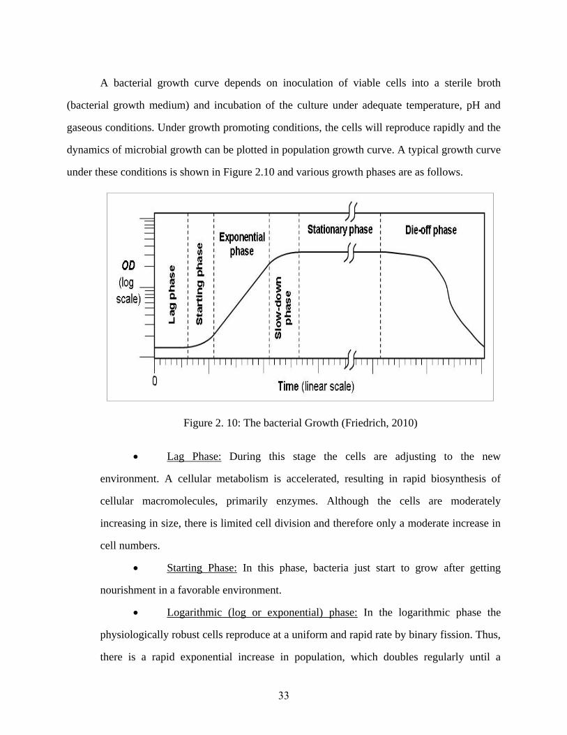
33
A bacterial growth curve depends on inoculation of viable cells into a sterile broth
(bacterial growth medium) and incubation of the culture under adequate temperature, pH and
gaseous conditions. Under growth promoting conditions, the cells will reproduce rapidly and the
dynamics of microbial growth can be plotted in population growth curve. A typical growth curve
under these conditions is shown in Figure 2.10 and various growth phases are as follows.
Figure 2. 10: The bacterial Growth (Friedrich, 2010)
Lag Phase: During this stage the cells are adjusting to the new
environment. A cellular metabolism is accelerated, resulting in rapid biosynthesis of
cellular macromolecules, primarily enzymes. Although the cells are moderately
increasing in size, there is limited cell division and therefore only a moderate increase in
cell numbers.
Starting Phase: In this phase, bacteria just start to grow after getting
nourishment in a favorable environment.
Logarithmic (log or exponential) phase: In the logarithmic phase the
physiologically robust cells reproduce at a uniform and rapid rate by binary fission. Thus,
there is a rapid exponential increase in population, which doubles regularly until a
34
maximum number of cells are reached. The length of the log phase depends on the
organisms and the composition of the medium and varies significantly depending on
bacteria type.
Stationary Phase: During this stage, the number of cells undergoing
division is equal to the number of cells that are dying. Therefore there is no further
increase in cell number, and the population is maintained at is maximum level for a
period of time. The primary factors responsible for this phase are the depletion of some
essential nutrients and the accumulation of toxic acidic or alkaline waste products in the
medium.
Decline or Death Phase: Because of the continuing depletion of nutrients
and buildup of metabolic wastes, the microorganisms die rapidly at a uniform rate. The
decrease in bacteria population closely parallels to its increase during the log phase.
Theoretically, the entire population should die during a time interval equal to that of the
log phase. Since a small number of highly resistant organisms persist for an indeterminate
length of time, this does not happen.
Slow-down Phase: In this phase, bacteria just start dying due to lack of
nutrients.
2.3.3 Microbiologically Induced Carbonate Precipitation (MICP)
Carbonate precipitation is a common natural phenomenon found in the environment.
According to Boquet et al. (1973), calcium carbonate is a general phenomenon in the bacterial
world, and under suitable conditions, most bacteria are able to precipitate calcite crystals.
Precipitation of CaCO3 can occur in two ways: abiotic and biotic pathways. Abiotic precipitation
occurs in supersaturated solutions through evaporation, temperature increases, and pressure
decreases (Castanier et al., 1999). Biotic precipitation can be either biotically controlled or
biotically induced. When an organism exerts some sort of control over the location, size, and
composition of the minerals formed, like skeletons and shells, the process is said to be biotically
35
controlled (Frankel et al., 2003). If the precipitation arises as a result of the metabolic activity of
an organism, and the organism has little or no control over the mineralization, the process is
biotically induced (Frankel et al., 2003). Carbonate precipitation has great importance in many
environmental and civil engineering (material) applications. Abiotic precipitation has been used
for purposes as wide ranging as permeability reduction in unconsolidated soils (Bird et al., 2008)
to methods for carbon dioxide disposal (Lackner et al., 1995). Biologically induced carbonate
precipitation by bacteria has been proposed for several biotechnological applications.
Carbonate mineralization by bacteria can occur in two ways: active or passive pathways.
Active precipitation occurs as a by-product of common microbial processes such as
photosynthesis, urea hydrolysis, sulfate reduction, and iron reduction (Knorre et al., 2000).
Actually these processes increase the pH in the environment surrounding the bacteria that alters
the saturation state of carbonate and other ions, such as calcium and iron. These new saturation
states allows carbonate to precipitate out of solution as calcium carbonate (calcite, aragonite, or
vaterite), magnesite, siderite, dolomite, or any number of carbonate minerals. One engineering
application for active carbonate precipitation is the use of iron (III) reducing bacteria to stabilize
fly ash, a residue generated by the combustion of coal, into siderite (FeCO3) and calcite (CaCO3)
(Roh et al., 2001).
In passive carbonate precipitation, heterogeneous nucleation on negatively charged points
of bacteria attracts positively charged ions, allowing for the precipitation of carbonate
(Bazylinski et al., 2003). Calcium carbonate is one of the most common products of carbonate
precipitation, as both calcium and carbonate ions are abundant in natural environments.
Bacteria used in this study are Bacillus Pasteuri, a urea hydrolyzing bacteria known for
their calcite precipitation. Carbonate mineralization of these bacteria follows active pathways.
The process is fairly straightforward. In the first step, bacteria get nutrition from culture medium
and secrete urease enzyme (Urea-amino-hydrolease), this enzyme hydrolyzed urea (CO(NH2)2)
to ammonia (NH3) and carbonic acid (H2CO3) in the series of reactions outlined bin equations 2-
4 through 2-6 (Burne et al., 2000). Then this ammonia and carbonic acid equilibrate in water to

36
form bicarbonate (HCO3-), ammonium (NH4
+), and hydroxide ion (OH
-) (Equations 2-7 & 8).
After this, the pH increase due to formation of NH4+ which is essential for creation of calcite.
This rise in pH shifts the bicarbonate equilibrium to form carbonate ions (CO32-
) (Equation 2-9)
which, in the presence of soluble calcium (Ca2+
), precipitates out of solution as calcium
carbonate (CaCO3) if saturation is exceeded (Burne et al., 2000; Castanier et al., 1999). The
overall reaction from the hydrolysis of urea in the presence of calcium is listed in the following
equations.
2- 4
2- 5
(Overall, step 1)
2- 6
2- 7
2- 8
2- 9
2- 10
(Overall process)
2- 11
Urease enzyme (catalyst)
37
These reactions occur under the influence of natural environmental factors. These factors
are the type of bacteria; bacteria cell concentration, temperature, urea concentration, calcium
concentration, ionic strength, and the pH of the media. Also the activity of the urease enzyme is
controlled by these factors and may have a significant impact on microbial carbonate
precipitation. The bacteria should possess high ureolytic efficiency, alkalophilic (optimum
growth rate occurs at pH around 9, and no growth at all around pH 6.5), non-pathogenic, and
possess the ability to deposit calcite homogeneously on the substratum (George et al., 2010). The
bacteria should also have a high negative zeta-potential (Dick et al., 2006) to promote adhesion
and surface colonization, and produce enormous amounts of urease enzyme in the presence of
high concentrations of ammonium (Kaltwasser et al., 1972) to enhance both the rate of ureolysis
and microbial carbonate precipitation (Nemati et al., 2003).
Urease-catalyzed ureolysis is also influenced by temperature like any other enzymatic
reaction. The optimum temperature ranges from 20 to 37
C depending on environmental
conditions and concentrations of other reactants in the system (George et al., 2010). It has been
reported that the rate of ureolysis increases with temperature, when temperature rises from 15 to
20 C, the rate of ureolysis kurea is 5 to 10 times greater from 10
C (Mitchell et al., 2005). Thus,
the rate of ureolysis can be enhanced by increasing the temperature within the optimum range.
Nemati and Voordouw (2003) verified that increasing urea and Ca2+
beyond 36 and 90g
L-1
, respectively, does not have any significant effect on bacterial calcium carbonate
precipitation. Since Ca2+
is not utilized by microbial metabolic processes, it would accumulate
outside the cell where it would be readily available for MCP (Silver et al., 1975).
Ionic strength is also an important factor which influences enzymatic reactions like
temperature and concentration. In bacteria transport of porous media, the total interaction energy
needed by microbial particles to adhere and attach themselves to solid surfaces as explained by
the classical Derjaguin– Landau–Verwey–Overbeek theory, is composed of the repulsive
electrostatic forces and the attractive Van Der Waals forces (George et al., 2010). High ionic
strength increases electrical double layer (EDL) compression by decreasing EDL repulsive
38
forces leaving attractive Van Der Waals forces to dominate, and in the process promotes
bacterial adhesion and attachment to the substratum (Faibish et al., 1998). Martell and Smith
(1974) showed that the equilibrium constant for ammonia speciation increase from 9.3 to 9.4 by
raising ionic strength from 0.1 to 1.0.
A pH increase is an indication of urea hydrolysis, and is an important property of
alkalophiles (optimum growth at pH 9 and no growth below pH 6.5). At any pH levels, NH3 gas
and dissolved NH4+ exist at different concentrations. A higher concentration of NH3 creates
favorable conditions for microbial carbonate precipitation (George et al., 2010).
2.3.4 Biocementation in Concrete
Use of microorganisms within mortar or PCC leading to the process of carbonate
biomineralization is now a potential field of research in concrete technology (Ramachandran et
al., 2001). Recently, an inherent cement based biomaterial has been developed to remediate the
cracks and fissures in concrete structures. Previous studies have shown that the addition of
specific microorganisms to cement–sand mortar or PCC deposits inorganic substances inside the
pores of the matrices, which can be used as a filling material to remediate cracks within the
structures (Ghosh et al., 2005). It was also noted that the addition of an anaerobic hot spring
bacterium (closely related to Shewanella species) to the mortar/PCC could increase the
compressive strength (25–30%) of the material with respect to control specimens (Ghosh et al.,
2006). Achal et al. (2010) have found no significant influence on compressive strength of mortar
samples without bacteria due to curing on water or nutrient broth urea medium. Park et al. (2009)
performed recent research to investigate the impact on compressive strength of four different
calcite forming strains of bacteria Sporosarcina soli, Bacillus massiliensis, Arthrobacter
crystallopoietes and Lysinibacillus fusiformis. Among those strains, samples treated with
Arthrobacter crystallopoietes had shown 8.9 percent more compressive strength than the control
specimen. Bacteria cell concentrations also significantly affect the compressive strength of
mortar samples. It has been found that bacteria treated mortar or PCC specimens will reach

39
maximum compressive strength for an optimum cell concentration (Ghosh et al., 2009). Recent
research showed that bacteria can survive better in fly ash amended mortar due to more number
of finer pores that provide better aeration to bacteria for better growth (Varenyam et al., 2011).
Bacteria count was greater in higher percentage fly ash. Another significant finding by
Varenyam et al. (2011) is that an optimum amount of fly ash and bacteria cells needs to be mixed
with specimens to achieve higher compressive strength. So, microbial modified mortar or PCC
has become an important area of research for high performance construction material.
The biologically induced cement based materials not only improve compressive strength
but also improve durability and performance compared to normal PCC materials. Verenyam et
al. (2011) examined the effect of absorption rate of fly ash and bacteria treated mortar and stated
that bacteria treated mortar absorbed 3.5 times less water than control specimens. Effect of
biodeposition on carbonation and chloride ingression in mortar was inspected by Muynck et al.
(2007). They found bacterial biodeposition slows carbonation and chloride ingression rate in
samples. Overall, bacterial cementation increases resistance of PCC specimens and retards the
process which leads to degradation.
With increase in construction, the production of PC has increased, which has led to a
higher carbon foot print. However, the use of byproduct fly ash and micro-organisms can lower
required PC content, thus minimizing the carbon footprint while increasing strength and
durability.
2.3.5 Conclusion
The hydrolysis of urea by urease enzyme is special in the sense that it is one of the few
biologically occurring reactions that produce carbonate ion and as a result precipitate calcium
carbonate, a solid crystalline mineral in a calcium rich environment. The binding strength of the
precipitated crystal is highly dependent on the factors influencing reactions and activity of urease
enzyme that control the rate of carbonate formation. Under suitable condition the yield of these
reactions is hard binding calcite cement (or Biocement).
40
However, it is very difficult for microorganism to survive in mortar or PCC due to high
pH surrounding the environment. Also, inclusion of brine or salt material as an alternative and
partial replacement of sand raises the pH of the specimen, which causes death of bacteria. That is
why bacteria or microorganisms mutate to live in a high pH environment. Beside this, fly ash
lowers the pH of PCC or mortar, as it transforms calcium hydroxide to C-S-H adhesive gel.
The main objective of this research is to find a sustainable environmentally friendly way
to dispose of concentrate brine in civil infrastructure like highways and as a building material.
One of the most promising ways to dispose of concentrated brine in cement mortar or PCC is
addition of fly ash and microbial carbonate precipitation, as these carbonates will plug the pores
in mortar or PCC top surfaces, which will later prevent the leaching of salt when it comes in
contact with water. Furthermore, this mineralization process will increase the compressive
strength of mortar or PCC and compensates for the inclusion of chloride ions in the solution,
which is known to weaken the integrity of the cement matrix.

41
Chapter 3: Experiment Design and Evaluation Tests
To determine the effect of adding TDS, bacteria, and fly ash on strength and durability of
mortar, an experiment design was developed to evaluate the influence of the proposed additives.
The impact of additives in terms of change in strength and durability of mortar was evaluated
using standard test methods. The influence of additives was evaluated by performing macro level
tests and verified using micro level tests. In this chapter, the proposed experiment design, test
methods for performance evaluation, and employed specimen preparation techniques are
discussed. Since use of bacteria is infrequent in civil infrastructure, a brief discussion on bacteria
growth is also presented.
3.1 Experiment Design
To develop test matrix, an initial investigation was performed to identify suitable amount
of sand that can be replaced by salt/TDS. The evaluation was performed by replacing percent of
sand with salt similar to the one performed for replacing cement with fly ash. The investigation
identified that more than 5% replacement of sand with salt reduces strength significantly
(crumbling of specimen under loading). Although addition of fly ash and bacteria will improve
the strength, the durability will be an issue. Therefore, it was decided to replace only 5% of sand
with salt. Since mortar consisting of bacteria requires use of phosphate buffer (discussed in detail
in culture of bacteria section), an initial investigation was conducted to identify influence of
sodium phosphate buffer instead of water on strength gain. The results of investigation indicated
that influence of phosphate buffer is insignificant. Therefore, mortar specimens were prepared
using sodium phosphate buffer for strength and durability evaluation. In addition, fly ash was
used to reduce amount of PC and improve the survivability of bacteria.
The strength and durability tests performed for evaluating sustainable disposal of salts are
summarized in Table 3.1 and amount of each component for testing is shown in Table 3.2. The
compressive strength, absorption, and freeze thaw tests were performed on 2 in. cube specimens
while permeability tests were performed on 4x4 in. specimens. To minimize the number of tests,

42
the strength tests were initially performed and components meeting or exceeding control
specimen strengths were evaluated for durability; therefore, numbers of specimens for durability
tests are significantly lower than for compressive strength tests. In addition, strength of mortar
was evaluated by performing tests after 3, 7, and 28 days of curing. To evaluate influence of each
component on strength and durability, two specimens were prepared and tested for permeability
testing and three specimens were prepared and tested for remaining tests.
The specimens were prepared by maintaining a Cement-Sand-Water ratio of 1-2.75-
0.485. The amount of each component is shown in Table 3.2. The amount of each component for
2 in. cube specimens is for six specimens, while the amount of each component for cylindrical
specimens is for one specimen. The strength evaluation of various fly ash contents indicated that
an increase in fly ash of more than 5% negatively impacted strength. Therefore, only 5% of fly
ash content was evaluated for durability and bacteria evaluation. The influence of bacteria on
mortar performance was evaluated using Bacillus pasteurii (BP) as well as mutated Bacillus
pasteurii (MB).
Table 3. 1: Specimen Size and Tests Performed
Specimen Shape
Dimensions (in.) Number of Specimens
Test Performed Length/
Diameter Width Height
Cube 2 2 2 117 Compressive Strength
(ASTM C109-08)
Cube 2 2 2 18 Freeze Thaw
(ASTM C1645M-09)
Cube 2 2 2 18 Absorption
(ASTM C1585-11)
Cylinder 4 - 4 12 Water Permeability
(CRDC-C 163-92)

43
Table 3. 2: Amount of Mortar Components
Specimen Size
Mortar Components
Material Amount
Cement (C),
grams
Fly Ash(F), grams
Sand (S),
grams
Salt (St),
grams
Water (W), ml
Phosphate Buffer (P),
ml
Amount of Materials required for Six-2 in. Cube
Specimens
CSW 500 --- 1,375.0 --- 242.5
CSP 500 --- 1,375.0 --- --- 242.5
CSSP5% 500 --- 1,306.3 68.7 --- 242.5
CSFP5% 475 25 1,375.0 --- --- 242.5
CSSFP5% 475 25 1,306.3 68.7 --- 242.5
CSFB5% 475 25 1,375.0 --- --- 242.5
CSMB 500 25 1,375.0 --- --- 242.5
CSFMB5% 475 25 1,375.0 --- --- 242.5
CSSFMB5% 475 25 1,306.3 68.7 --- 242.5
CSFP10% 450 50 1,375.0 --- --- 242.5
CSFP20% 400 100 1,375.0 --- --- 242.5
CSFP30% 350 150 1,375.0 --- --- 242.5
CSFP40% 300 200 1,375.0 --- --- 242.5
Amount of Material required for one 4x4 in
Cylinder Specimen
CSP 415 --- 1,142.0 --- --- 201.0
CSFP5% 394 21 1,142.0 --- --- 201.0
CSSFP5% 394 21 1,085.0 57 --- 201.0
CSFB5% 394 21 1,142.0 --- --- 201.0
CSFMB5% 394 21 1,142.0 --- --- 201.0
CSSFMB5% 394 21 1,085.0 57 --- 201.0

44
3.2 Culture of Bacteria
3.2.1 Introduction
Bacterial induced carbonate mineralization (a.k.a. Biocementation) has been
demonstrated as a new additive to improve the strength and performance of mortar or concrete.
Park et al. (2009) established that bacteria strains like Arthrobacter crystallopoietes (ATCC
15481), Sporosarcina pasteurii (ATCC 11859), Bacillus sphaericus (ATCC 14577), and
Lysinibacillus fusiformis (ATCC 7055) etc. have enough potentiality to precipitate calcium
carbonate in optimum condition. For this research, a vial of Sporosarcina pasteurii or Bacillus
pasteurii (BP) was procured from American Type Culture Collection (ATCC). This vial of BP
was then cultured to multiply microbial organisms by letting them reproduce in a conducive
medium under controlled laboratory conditions.
3.2.2 Constituents Required for Bacteria Growth
In this section, various chemicals used to culture Bacillus pasteurii bacteria (also known
as wild BP) and nutrients required during curing of mortar are discussed. The constituents and
their compositions of the medium were maintained constant throughout the study to nullify the
influence of changes in chemicals on the growth of bacteria. For MB, a higher pH was
maintained to improve the survivability and minimize mutation reversal of bacteria.
3.2.2.1 Chemicals for Growth of Bacteria and Curing of Mortar
Various chemicals were used to the prepare medium for growth and isolation of bacteria.
The culture medium for growth is prepared by mixing Yeast extract (Sigma Aldrich; product
no.Y1001), Tris Buffer (Sigma Aldrich; product no. T6066), and Ammonium Sulfate
((NH4)2SO4¬, Sigma Aldrich; product no.A2939). The amounts of ingredients required for
optimal growth are shown in Table 3.3. After growth of bacteria, the culture medium is washed
(using sodium phosphate buffer) to remove chemicals used for bacteria growth and adjusted for
required Optical Density of bacteria. The buffer was prepared by mixing 8.2 grams of Sodium
Phosphate (Na3PO4, Sigma Aldrich; product no. 342483) in 1 liter of water.

45
Table 3. 3: Ingredients of Tris-YE bacteria Culture Medium
3.2.2.2 Growth of Bacillus Pasteurii
Bacillus pasteurii (ATCC 11859) was used throughout the specimens preparation. A
medium (Tris-YE) was used for stock and pilot cultures of B. Pasteurii. This medium was
prepared following ATCC Medium 1376 protocol.
Individual ingredients (shown in Table 3.1) were autoclaved aseptically (free of
pathogenic microorganism) in a cell culture hood (Figure 3.1) and combined afterwards to avoid
precipitation of ingredients. Each ingredient was mixed in 1/3 liter of deionized water and
autoclaved. In the autoclave, a high pressure stream of 2.9 psi/ minute was applied at 121° C for
around 15-20 minutes depending on the size of the loads and the contents. At this stage, the pH
of the culture medium is approximately 9.0. The culture medium obtained from this process is
termed Tris-Yeast medium. A small amount of BP was taken from the vial and cultured in 100
ml Tris-Yeast medium at 30 ºC under aerobic conditions and incubated in a shaker operated at
200 rpm for 24 hours (Figure 3.2). The bacteria and the culture medium were either frozen for
future use or washed using sodium phosphate buffer to prepare specimens. To prepare frozen
stock of BP strain for future use, 0.5 ml. of culture medium (which includes bacteria) sample
were aliquoted and mixed with 0.5 ml. of 15% glycerol. This mixture was frozen at -70 ºC to be
used in the future for growth of bacteria.
Ingredient Amount per liter
Yeast Extract 20 g
Ammonium Sulfate, (NH4)2SO4 10 g
0.13 M Tris Buffer (pH 9.0) 15.75 g

46
The culture medium obtained after 24 hour shaking was poured in a container and
centrifuged at 4,000 rpm for 15 minutes to precipitate bacteria at the bottom of the container,
which is commonly known as harvesting cell pellets. These cell pellets were then washed twice
with 50 milliMolar sodium phosphate buffer containing 8.2 gm. of sodium phosphate per liter
(pH 7.5) of water. The final cell pellets were then suspended in phosphate buffer and adjusted to
obtain desired optical density using a Spectrophotometer (Figure 3.3). This bacteria suspension
was used for preparing specimens.
Figure 3. 1: Cell Culture Hood (Labgard, Class-II, Type A2)
Figure 3. 2: Shake Incubator

47
Figure 3. 3: Spectrophotometer
3.2.2.3 Mutation of Bacteria
B. Pasteurii grows well at an optimum pH of 9.0 and also has the capability to produce
the endospore. Endospore is a dormant form of the cell to endure extreme environments.
However, higher pH of PCC and increase in osmotic pressure of bacteria in the presence of salt
reduces survivability of bacteria and urease activity. Achal et.al (2009) investigated that ultra
violet (UV) irradiation of BP not only increased the efficiency of this bacterium to grow at high
pH but also increased urease activity for more calcite formation.
It has been found that UV light is to be lethal and mutagenic in a variety of organisms
including bacteria (Auerbach, 1976; Witkin, 1976). It is generally accepted that exposing
bacteria to UV irradiation results in DNA mutation by changing its DNA structure, which allows
bacteria to survive under adverse conditions (Miguel et al., 1983).
To obtain mutated bacteria, the BP was cultured in the regular growth medium as
described in section 3.1.3. After 24 hrs of incubation, this bacterial culture was exposed to UV
irradiation using a Philips 20W germicidal lamp (Figure 3.4) for 20 minutes. According to Achal
et al. (2009), a typical survival rate of less than 10% was observed. A small portion (1 ml) of
irradiated bacteria culture was randomly selected and transferred to a 100 ml of Tris-YE media
to grow the MB for 48 hours rather than 24 hours (for BP) in a shaker operated at 200 rpm 30 ºC
under aerobic conditions. To minimize reverse mutation, higher pH is required. Therefore, 4
molar sodium hydroxide (NaOH) was added to Tris-YE medium to increase pH from 9.0 to 10.5.
48
This process was repeated three times and each time samples were randomly selected from
immediate previous culture of MB. The purpose of culturing MB several times was to make sure
that MB is incapable of mutation reversal. Similar to BP, MB were frozen for future use or
washed for immediate sample preparation.
Figure 3. 4: Germicidal Lamp
3.3 Mortar Ingredients and Properties
This section gives an outline of various ingredients used in the preparation of cement
mortar samples. The source of materials was kept constant throughout the study so as to nullify
the influence of change in materials on the physical, mechanical, and durability characteristics of
mortar.
3.3.1.1 Portland Cement
Commercially available Type I/II Portland Cement was used throughout the study. Table
3.4 and Figure 3.5 summarize the chemical properties of cement.

49
Table 3.4: Main Constituents in a typical Portland cement (adapted from Mindess and
Young, 1981)
Chemical Name Chemical Formula Shortha
nd Notation Percent
by Weight
Tricalcium Silicate C3S 50
Dicalcium Silicate C2S 25
Tricalcium Aluminate C3A 12
Tetracalcium Aluminoferrite C4AF 8
Gypsum ̅ 3.5
Figure 3. 5: Typical Oxide Composition of a General-Purpose Portland Cement (adapted
from Mindess and Young, 1981)

50
3.3.1.2 Fine Aggregate
Quickrete-All Purpose Sand was used as fine aggregate in the experimental program. The
sand conform ASTM C 778 and its gradation is shown in Table 3.5.
Table 3. 5: Sieve Analysis of Fine Aggregate
Sieve No. Cumulative passing (%)
No. 16 (1.18 mm) 100
No. 30 (600 µm) 79
No.40 (425 µm) 57
No.50 (300 µm) 32
No.100 (150 µm) 6
3.3.1.3 Fly Ash
A commercially available Class F fly ash was used in some of the mixtures as a partial
replacement of cement, investigated to ascertain its impact on mechanical properties and
durability. A detail scanning electron microscopy (SEM), X-Ray diffraction analysis (XRD) will
be shown in the results and discussion section.
3.3.1.4 Water
In some mortar mixes, tap water from the city water network of El Paso was used.
3.3.1.5 Sodium Phosphate Buffer
Sodium phosphate buffer (SPB) of pH 7.5 was used in most of the mortar mixes. This
buffer contains 8.2 gm of Sodium Phosphate (Na3PO4) per liter of distilled water. The main
reason of choosing sodium phosphate buffer is that bacteria cannot survive in water because of a
difference in osmotic pressure and its cell will eventually lyse. Also, the existence of sodium
phosphate in water does not affect the water to cement ratio in mortar significantly.
51
3.3.1.6 Salt
The salt was obtained from RO concentrate that was collected from the KBH Desalting
Plant in El Paso, TX and was grounded and sieved using a No. 16 sieve (1.18 mm). Only the salt
particles passing through the No. 16 sieve were used as a partial replacement of sand (or fine
aggregate). A chemical analysis of the concentrate (from which the salt was obtained) was
performed by El Paso Water Utilities and is shown in Table 3.6. The results indicate that a major
portion of the TDS is sodium chloride. In addition, SEM and XRD analysis were performed and
are discussed in Chapter Four.
3.2.2 Mix Proportion and Specimen Preparation
This section describes the mixture proportions, mixing procedure and the method of
preparing specimens for testing the mechanical property, durability and micro level examination.
3.2.2.1 Sample Preparation
To evaluate strength and durability of mortar, 2 in. cubical and 4x4 in. cylindrical
specimens were prepared. Since strength was main criterion, the cubical specimens were
prepared according to ASTM C-109-2008 procedure. The procedure proposes to use tamping rod
25 times to prepare specimens of consistent density. The cylindrical specimens were prepared in
two layers and each layer was prepared by tamping 25 times. A standard mortar proportion of
one part of cement to 2.75 parts of standard sand by weight, and cement to water or sodium
phosphate buffer (SPB) of 0.485 was maintained throughout all sample preparation. The SPB is
similar to the one used for washing of bacteria as discussed in Section 3.3.1.5. When a fly ash
amended mortar was prepared, cement was partially replaced with fly ash in such a way that the
total weight of cement and fly ash was equivalent to the amount of cement required for normal
mortar. In similar manner, the salt amount was adjusted to prepare specimens consisting of salt.
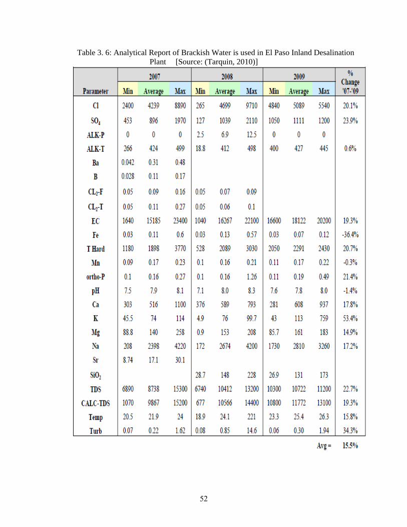
52
Table 3. 6: Analytical Report of Brackish Water is used in El Paso Inland Desalination
Plant [Source: (Tarquin, 2010)]
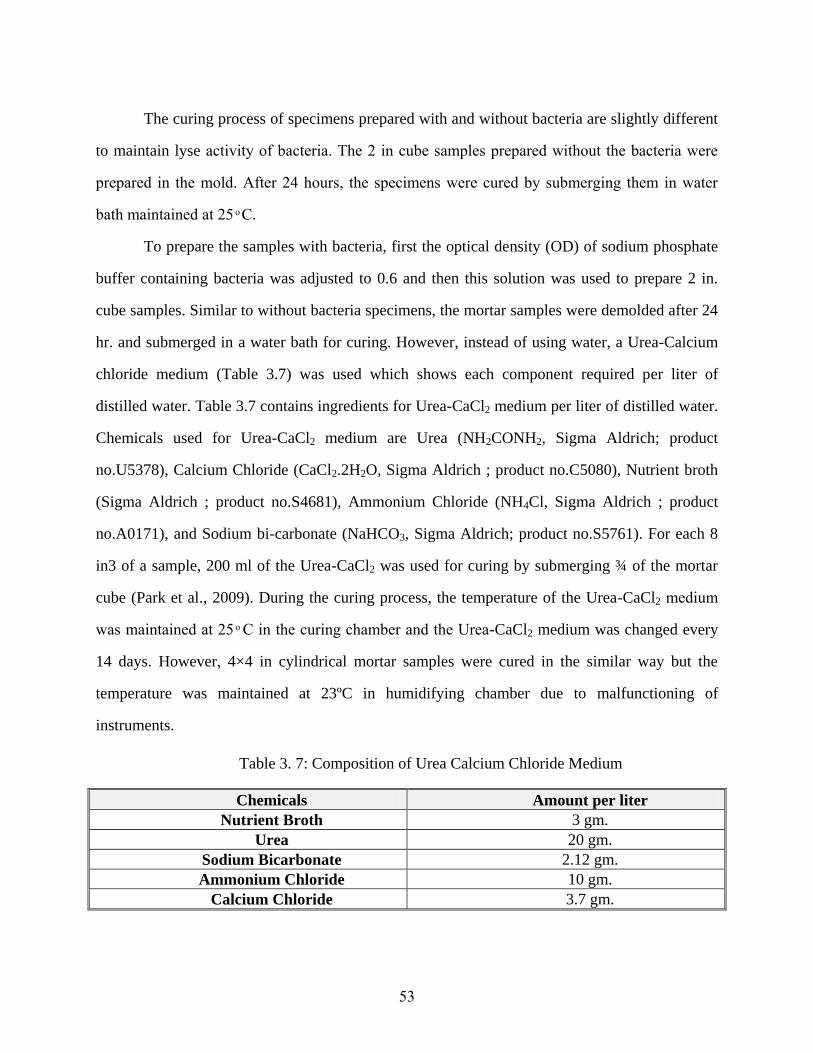
53
The curing process of specimens prepared with and without bacteria are slightly different
to maintain lyse activity of bacteria. The 2 in cube samples prepared without the bacteria were
prepared in the mold. After 2 hours, the specimens were cured by submerging them in water
bath maintained at 2 C.
To prepare the samples with bacteria, first the optical density (OD) of sodium phosphate
buffer containing bacteria was adjusted to 0.6 and then this solution was used to prepare 2 in.
cube samples. Similar to without bacteria specimens, the mortar samples were demolded after 24
hr. and submerged in a water bath for curing. However, instead of using water, a Urea-Calcium
chloride medium (Table 3.7) was used which shows each component required per liter of
distilled water. Table 3.7 contains ingredients for Urea-CaCl2 medium per liter of distilled water.
Chemicals used for Urea-CaCl2 medium are Urea (NH2CONH2, Sigma Aldrich; product
no.U5378), Calcium Chloride (CaCl2.2H2O, Sigma Aldrich ; product no.C5080), Nutrient broth
(Sigma Aldrich ; product no.S4681), Ammonium Chloride (NH4Cl, Sigma Aldrich ; product
no.A0171), and Sodium bi-carbonate (NaHCO3, Sigma Aldrich; product no.S5761). For each 8
in3 of a sample, 200 ml of the Urea-CaCl2 was used for curing by submerging ¾ of the mortar
cube (Park et al., 2009). During the curing process, the temperature of the Urea-CaCl2 medium
was maintained at 2 C in the curing chamber and the Urea-CaCl2 medium was changed every
14 days. However, 4×4 in cylindrical mortar samples were cured in the similar way but the
temperature was maintained at 23ºC in humidifying chamber due to malfunctioning of
instruments.
Table 3. 7: Composition of Urea Calcium Chloride Medium
Chemicals Amount per liter
Nutrient Broth 3 gm.
Urea 20 gm.
Sodium Bicarbonate 2.12 gm.
Ammonium Chloride 10 gm.
Calcium Chloride 3.7 gm.
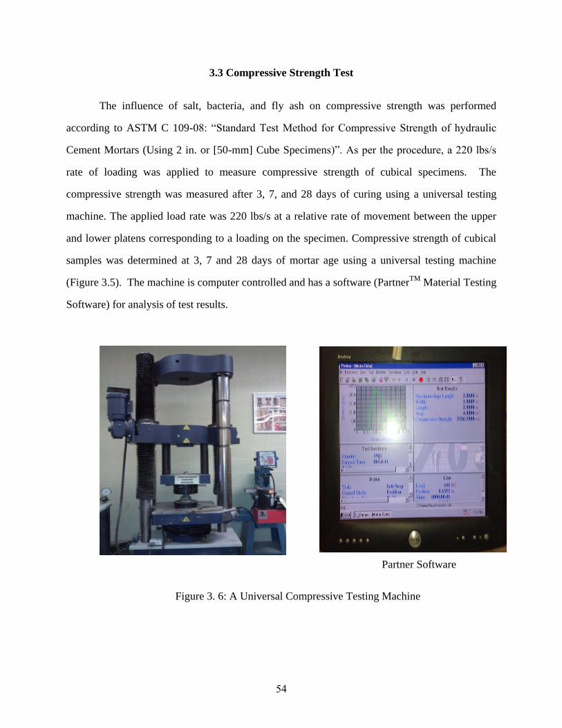
54
3.3 Compressive Strength Test
The influence of salt, bacteria, and fly ash on compressive strength was performed
according to ASTM C 109-08: “Standard Test Method for Compressive Strength of hydraulic
Cement Mortars (Using 2 in. or [50-mm] Cube Specimens)”. As per the procedure, a 220 lbs/s
rate of loading was applied to measure compressive strength of cubical specimens. The
compressive strength was measured after 3, 7, and 28 days of curing using a universal testing
machine. The applied load rate was 220 lbs/s at a relative rate of movement between the upper
and lower platens corresponding to a loading on the specimen. Compressive strength of cubical
samples was determined at 3, 7 and 28 days of mortar age using a universal testing machine
(Figure 3.5). The machine is computer controlled and has a software (PartnerTM
Material Testing
Software) for analysis of test results.
Figure 3. 6: A Universal Compressive Testing Machine
Partner Software

55
3.4 Durability Tests
Durability is the ability of material to last long time without significant deterioration.
Durability of concrete has been defined by American Concrete Institute as its resistance to
weathering action, chemical attack, abrasion and other degradation process. Concrete elements
always are subjected to synergistic effects of the environmental and mechanical loads. This study
is undoubtedly meaningful and critical to ensure safety, durability as well as life prediction of
concrete material.
Durable materials have a significant positive effect on the environment by conserving
limited natural resources, reducing wastes, and minimizing repair and replacement. The purpose
of performing a durability test is to ensure that the addition of salts does not significantly
influence the performance life of mortar exposed to severe weather conditions. Different
durability tests had been performed in this research to evaluate the impact of by-product fly ash
and salt while partially replacing cement and sand, respectively. In the following sections,
freeze-thaw, absorption, and permeability tests followed for durability evaluation are described.
3.4.1 Freeze Thaw Test
The purpose of freeze thaw test method is to evaluate the resistance to freezing and
thawing of solid interlocking concrete paving units. The test method followed ASTM C 1645M-
09: “Standard Test Method for Freeze-thaw and De-icing Salt durability of Solid Concrete
Interlocking Paving Units”. This procedure measure the amount of scaling per unit surface area
owing to a number of well-defined freezing and thawing cycles in the presence of test solution
(tap water). For freezing and thawing the 2 in cube samples, the climatic chamber used in this
experiment is shown in Figure 3.7.

56
Figure 3. 7: Environmental Chamber
The following test conditions were applied for freeze thaw test:
According to ASTM C 1645M-09, the sample thickness should be at least 2.36 in.
and surface area of 29.5 in2. However, the cubical specimen prepared for
durability tests have thickness of 2 in, and surface area of 24 in2. Since strength
tests were performed on 2 in. cubical specimens, it was decided to perform freeze
thaw tests on same size specimens.
Since durability is evaluated to identify long term performance, the test specimens
were cured for 28 days as specified in the strength test section before subjecting
them to freeze thaw cycling.
The procedure suggests additional curing options of 28 days (i.e., 56 days of
curing) which was not followed due to time constraints of the project.
The specimens were allowed to air cure for 48 h in an environmental chamber at
25 ºC. Although the procedure suggests maintaining more than 80% of relative
humidity, the specimens were not exposed to higher relative humidity due to
malfunction of the chamber.
One cycle of freeze thaw consists of 16±1 h of freezing followed by 8±1 h of
thawing. Each specimen was subjected to 28 continuous cycles i.e., 28 days of

57
freeze thaw. The temperature is maintained constant at -5 °C for freezing cycles
and at 5° C for thawing cycle.
Tap water was used as the test solution to collect residue. The specimens were
washed using water to remove loose particles. These particles and spall material
from specimens was filtered after 7 and 28 cycles. The filtering was done using
filter paver with a maximum opening of 80 µm.
The residues were dried in an oven for at least 4h until two successive weighing at
2h intervals didn’t show loss more than 0.2% of the last previously determined
weight.
3.4.2 Water Permeability Test
The purpose of this test method is to determine the water permeability of concrete or
mortar using a triaxial cell. This test procedure followed CRD-C 163-92: “Test Method for
Water Permeability of Concrete using Triaxial Cell”. Initially a radial confining pressure is
applied around the specimen housed in a triaxial permeability cell. Then a pressure gradient is
maintained between one end exposed to ambient pressure and the other end at the test drive
pressure in order to establish a steady state flow condition in a cylindrical concrete specimen.
The influent (i.e. water) was measured to calculate volume flow rate. Once steady state
conditions were obtained, the intrinsic permeability was calculated. In the following Figures 3.8
and 3.9 the test configuration is shown.

58
Figure 3. 8: Schematic diagram of Test configuration
Figure 3. 9: Experimental Setup of Water Permeability Test
Air Gas Source
Triaxial Permeability Cell
Pressure Regulating
Valve

59
The water permeability test conditions are as followed:
The 4 4 in. cylindrical specimens were completely submerged for 72 h in tap water to
saturate it, instead of doing vacuum saturated in deionized water.
According to the test procedure, the confining pressure shall be less than one-half of
unconfined compressive strength of the specimen and driving pressure. To test the
specimens, the confining and driving pressure was maintained 30 psi (207 KPa) and 20
psi (138 KPa) respectively.
Air gas source was used in lieu of compressed nitrogen gas to apply confining and
driving pressure.
During the experiments, the pressure was maintained within ±5% of the predetermined
levels by adjusting the pressure regulating valve.
Tap water was used as influent instead of using de-ionized water.
3.4.3 Absorption or Sorptivity Test
Sorptivity characterizes the material’s ability to absorb and transmit water through it by
capillary suction. So it is an important durability parameter for above ground structures. This test
is performed according to ASTM C1585-11: “Standard Test Method for Measurement of Rate of
Absorption of Water by Hydraulic-Cement Concretes”. This test method determines the rate of
absorption (i.e. sorptivity) of water by hydraulic cement concrete by measuring the increase in
the mass of a specimen resulting from absorption of water as a function of time when only one
surface of the specimen is exposed to water. The exposed surface is immersed in water and water
ingress of unsaturated concrete dominated by capillary suction during initial contact with water.
Figure 3.10 show the schematic of the testing procedure.
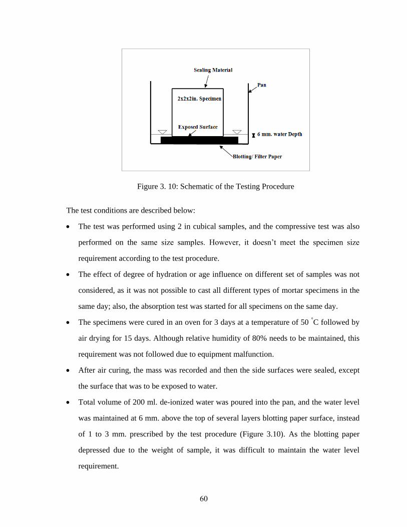
60
Figure 3. 10: Schematic of the Testing Procedure
The test conditions are described below:
The test was performed using 2 in cubical samples, and the compressive test was also
performed on the same size samples. However, it doesn’t meet the specimen size
requirement according to the test procedure.
The effect of degree of hydration or age influence on different set of samples was not
considered, as it was not possible to cast all different types of mortar specimens in the
same day; also, the absorption test was started for all specimens on the same day.
The specimens were cured in an oven for 3 days at a temperature of 50 °C followed by
air drying for 15 days. Although relative humidity of 80% needs to be maintained, this
requirement was not followed due to equipment malfunction.
After air curing, the mass was recorded and then the side surfaces were sealed, except
the surface that was to be exposed to water.
Total volume of 200 ml. de-ionized water was poured into the pan, and the water level
was maintained at 6 mm. above the top of several layers blotting paper surface, instead
of 1 to 3 mm. prescribed by the test procedure (Figure 3.10). As the blotting paper
depressed due to the weight of sample, it was difficult to maintain the water level
requirement.

61
The water level was kept constant by adding de-ionized water during the experiment.
The specimens were weighed at 1 min, 5 min, 10 min, 20 min, 30 min, 1 h, 2h, 3h, 4h,
5h, 6h and after 6h the reading was collected each day up to 8th
day after 24 h interval
following the test procedure.
Electrical conductivity (EC) and pH reading was taken at required intervals in addition
to mass reading.
A chemical analysis was performed by ion chromatography test to examine the leach
elements from the samples to water.
3.4.3.1 Ion Chromatography Test
Ion chromatography (IC) is a test method for ionic analysis of water samples. IC has been
incorporated into environmental regulatory methods for many standard organizations, such as
ASTM, ISO (International Organization of Standardization) etc. to examine contaminants in
drinking water, wastewater, surface and ground water, rain water, soil extracts, and other
environmental sample matrixes. IC is used to measure concentrations of major anions: fluoride,
chloride, nitrate, nitrite, and sulfate as well as major cations such as lithium, sodium, ammonium,
potassium, calcium and magnesium in the parts-per-billion (ppb) range. IC test was used to
determine the concentration of chloride, sulfate, sodium, potassium, calcium and magnesium
ions presence in water solutions of absorption test to detect leaching of elements from tested
mortar. Figure 3.11 and 3.12 show a typical ion chromatography system and schematic diagram
of ion analysis process through different stages, respectively.

62
Figure 3. 11: Ion Chromatography System
Figure 3. 12: Ion Analysis Process (Dionex ICS-2100 Ion Chromatography System
Operator)
The main working principle of IC system is to measure the ionic concentration of species
by separating them based on their interaction with a resin. Ionic species separate differently
depending on species type and size. Sample solutions pass through a pressurized
chromatographic column where ions are absorbed by column constituents. An extraction liquid
runs through the column to separate absorbed ions from the column. The separated ions are
ICS 2100 ECD ICS 1100 ECD

63
measured by their conductivity. They are identified on the basis of retention time as compared to
standards. Quantification is performed by peak area of peak height measurement. The overall
system is controlled by chromatography software named “Chromeleon ver. 6.8”. The results can
be obtained from an excel spreadsheet which is created by the software and it includes result
tables, chromatograph, calibration plots, spectra, audit trails, and even custom equations and
charts.
In this study, chloride (Cl-) anion was measured using US EPA 300.1 method and cations
sodium (Na), potassium (K), calcium (Ca) and magnesium (Mg) were quantified using ISO
14911-1 method.
3.5 Micro Level Tests
To verify results of macro test results and to identify changes in micro-sturcture, micro
level tests were performed. Investigation of different micro-structure characteristics such as
crystal structure, mineralogy, surface topography, and elemental analysis of materials were
performed using X-ray diffractometer (XRD) and scanning electron microscopy (SEM).
3.5.1 XRD Analysis
Structural characterization of the fly ash, salt (brine) and different mortar samples were
investigated using Bruker D8 Discover advance XRD (Figure 3.13). Cu Kα radiation of
wavelength λ=1. 06 Å was used to analyze fly ash, salt using 0.2 mm slit while fragment of
mortar was examined with 1mm diameter point focus adjustment in a scanning range 10-90º in
2θ scale at a rate º/min.

64
Figure 3. 13: Bruker D8 X-Ray Diffractometer
X-rays are electromagnetic radiation of wavelength varying from 0.1 Å to 100 Å. For
diffraction application, short wavelength X-rays, also called hard X-rays (0.1 Å to few Å), are
used (Introduction to X-ray diffraction, 2011). X-ray diffraction is a non-destructive technique
for characterizing the crystalline material. An X-ray beam, produced by the X-ray tube is
directed towards the sample. When the beam strikes the sample, diffraction occurs (Figure 3.14)
according to Bragg law (ASM Handbook) which is as follows:
(3. 1)
Where d is the inter-planar spacing, θ is the scattering angle, λ is the wavelength of X-ray
and n is an integer. Bragg condition is also the condition for constructive interference. Bragg law
is satisfied by varying the angle θ. The diffraction pattern is usually recorded as intensity versus
diffraction angle 2θ. The peak positions in the diffraction pattern are directly related to d and the
peak intensity depends on the atom in the diffracting plane.
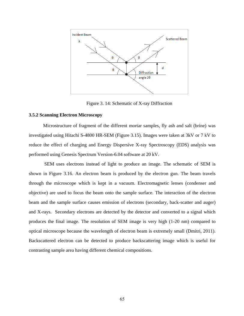
65
Figure 3. 14: Schematic of X-ray Diffraction
3.5.2 Scanning Electron Microscopy
Microstructure of fragment of the different mortar samples, fly ash and salt (brine) was
investigated using Hitachi S-4800 HR-SEM (Figure 3.15). Images were taken at 3kV or 7 kV to
reduce the effect of charging and Energy Dispersive X-ray Spectroscopy (EDS) analysis was
performed using Genesis Spectrum Version-6.04 software at 20 kV.
SEM uses electrons instead of light to produce an image. The schematic of SEM is
shown in Figure 3.16. An electron beam is produced by the electron gun. The beam travels
through the microscope which is kept in a vacuum. Electromagnetic lenses (condenser and
objective) are used to focus the beam onto the sample surface. The interaction of the electron
beam and the sample surface causes emission of electrons (secondary, back-scatter and auger)
and X-rays. Secondary electrons are detected by the detector and converted to a signal which
produces the final image. The resolution of SEM image is very high (1-20 nm) compared to
optical microscope because the wavelength of electron beam is extremely small (Dmitri, 2011).
Backscattered electron can be detected to produce backscattering image which is useful for
contrasting sample area having different chemical compositions.

66
Figure 3. 15: Hitachi S-4800 Scanning Electron Microscope
Figure 3. 16: Schematic of Scanning Electron Microscope
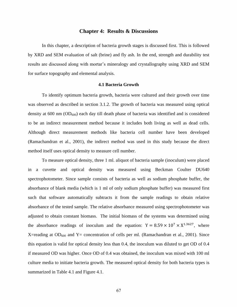
67
Chapter 4: Results & Discussions
In this chapter, a description of bacteria growth stages is discussed first. This is followed
by XRD and SEM evaluation of salt (brine) and fly ash. In the end, strength and durability test
results are discussed along with mortar’s mineralogy and crystallography using XRD and SEM
for surface topography and elemental analysis.
4.1 Bacteria Growth
To identify optimum bacteria growth, bacteria were cultured and their growth over time
was observed as described in section 3.1.2. The growth of bacteria was measured using optical
density at 600 nm (OD600) each day till death phase of bacteria was identified and is considered
to be an indirect measurement method because it includes both living as well as dead cells.
Although direct measurement methods like bacteria cell number have been developed
(Ramachandran et al., 2001), the indirect method was used in this study because the direct
method itself uses optical density to measure cell number.
To measure optical density, three 1 ml. aliquot of bacteria sample (inoculum) were placed
in a cuvette and optical density was measured using Beckman Coulter DU640
spectrophotometer. Since sample consists of bacteria as well as sodium phosphate buffer, the
absorbance of blank media (which is 1 ml of only sodium phosphate buffer) was measured first
such that software automatically subtracts it from the sample readings to obtain relative
absorbance of the tested sample. The relative absorbance measured using spectrophotometer was
adjusted to obtain constant biomass. The initial biomass of the systems was determined using
the absorbance readings of inoculum and the equation: , where
X=reading at OD600 and Y= concentration of cells per ml. (Ramachandran et al., 2001). Since
this equation is valid for optical density less than 0.4, the inoculum was diluted to get OD of 0.4
if measured OD was higher. Once OD of 0.4 was obtained, the inoculum was mixed with 100 ml
culture media to initiate bacteria growth. The measured optical density for both bacteria types is
summarized in Table 4.1 and Figure 4.1.

68
Table 4. 1: Optical Density (OD600) of Bacteria Samples
DDay
Normal Bacteria OD Average
OD Standard Deviation
Mutated Bacteria OD Average
OD Standard Deviation
00
Initially OD adjusted to 0.40 for 1 ml and then added to 100
ml Media
0.014 0
Initially OD adjusted to 0.40 for 1 ml and
then added to 100 ml Media
0.014 0
11
1.0996
1.0957 0.0042
0.0210
0.0238 0.0025 1.0963 0.0243
1.0912 0.0260
22
1.5478
1.5719 0.0368
1.0321
1.0052 0.0257 1.5536 1.0028
1.6142 0.9808
33
1.6557
1.6428 0.0127
1.0714
1.0853 0.0243 1.6423 1.0711
1.6304 1.1133
44
1.7115
1.6880 0.0293
1.1277
1.1433 0.0381 1.6973 1.1154
1.6551 1.1867
55
1.4976
1.4916 0.0215
1.2512
1.2400 0.0100 1.5095 1.2369
1.4678 1.2320
66
1.3755
1.4352 0.0561
1.3628
1.3984 0.0407 1.4868 1.4428
1.4432 1.3896
77
1.2471
1.2578 0.0092
1.2408
1.2446 0.0054 1.2631 1.2508
1.2631 1.2423

69
Figure 4. 1: Bacteria Growth Curve
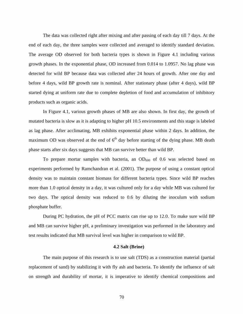
70
The data was collected right after mixing and after passing of each day till 7 days. At the
end of each day, the three samples were collected and averaged to identify standard deviation.
The average OD observed for both bacteria types is shown in Figure 4.1 including various
growth phases. In the exponential phase, OD increased from 0.014 to 1.0957. No lag phase was
detected for wild BP because data was collected after 24 hours of growth. After one day and
before 4 days, wild BP growth rate is nominal. After stationary phase (after 4 days), wild BP
started dying at uniform rate due to complete depletion of food and accumulation of inhibitory
products such as organic acids.
In Figure 4.1, various growth phases of MB are also shown. In first day, the growth of
mutated bacteria is slow as it is adapting to higher pH 10.5 environments and this stage is labeled
as lag phase. After acclimating, MB exhibits exponential phase within 2 days. In addition, the
maximum OD was observed at the end of 6th
day before starting of the dying phase. MB death
phase starts after six days suggests that MB can survive better than wild BP.
To prepare mortar samples with bacteria, an OD600 of 0.6 was selected based on
experiments performed by Ramchandran et al. (2001). The purpose of using a constant optical
density was to maintain constant biomass for different bacteria types. Since wild BP reaches
more than 1.0 optical density in a day, it was cultured only for a day while MB was cultured for
two days. The optical density was reduced to 0.6 by diluting the inoculum with sodium
phosphate buffer.
During PC hydration, the pH of PCC matrix can rise up to 12.0. To make sure wild BP
and MB can survive higher pH, a preliminary investigation was performed in the laboratory and
test results indicated that MB survival level was higher in comparison to wild BP.
4.2 Salt (Brine)
The main purpose of this research is to use salt (TDS) as a construction material (partial
replacement of sand) by stabilizing it with fly ash and bacteria. To identify the influence of salt
on strength and durability of mortar, it is imperative to identify chemical compositions and

71
mineralogy of salt with the help of XRD and SEM evaluation. The leaching of these elements
can be verified during durability evaluation of mortar specimens.
In section 3.3.1.6, the chemical analysis of this salt was summarized. The data indicated
presence of sodium (Na+), chlorine (Cl
-) as predominant elements while presence of calcium
(Ca2+
), sulfate (SO42-
), magnesium (Mg), potassium (K) and silica (SiO2) as minor elements. In
this study, XRD and SEM measurements were performed to verify presence of these elements.
4.2.1 XRD Analysis
As mentioned in Chapter 3, the salt obtained from plant was crushed and salt particles
passing through No.16 sieve were used for analysis. The XRD curve obtained for these salt
particles is shown in Figure 4.2. The XRD peaks observed can be indexed to that of halite (NaCl;
rock salt), which crystallizes in a cubic structure with a lattice parameter a= 5.6402 Å. In the
present work, the most intense peak appeared at 2θ=31.7896º. This peak corresponds to
diffraction from (200) planes of NaCl. The other NaCl peaks were observed at 2θ of 27.2994º,
45.4771º, 53.9542º, 56.4509º, 75.2898º and 84.0925º which corresponds to diffraction from
(111), (220), (311), (222), (420) and (422) crystal planes, respectively (Figure 4.2). The XRD
analysis suggests presence of different phases of NaCl in the tested sample.
4.2.2 SEM Analysis
The images of salt particles passing through No. 16 sieve were captured at 7 kV to
minimize influence of surface charging. In addition, energy dispersive X-ray spectroscopy (EDS)
analysis was performed, using Genesis Spectrum Version-6.04 software at 20 kV, to obtain
elemental information.

72
Figure 4. 2: XRD Pattern of Salt Particle

73
4.2.2.1 Surface Morphology of Salt
Surface morphology of salt can be seen from the representative SEM images shown in
Figure 4.3. The solid particles have smooth texture. It is clear that a large number of smaller
particles agglomerate over the surface of larger particles.
(a)
(b)
Figure 4. 3: SEM Image of Salt
4.2.2.2 EDS Analysis of Salt
The EDS spectra of salt is presented in Figure 4.4 and labeled with the elements detected
for corresponding X-rays. The intense peak of sodium and chlorine in EDS spectra verifies the
presence of significant amount of sodium chloride in salt samples also evidenced in XRD
analysis.
The elemental composition obtained from EDS is listed in Table 4.2. It is evident that the
major elements present are sodium and chlorine (more than 10 wt. %) which substantiates the
EDS spectra analysis, with minor elements magnesium, aluminum, silicon (1-10 wt. %). Also
calcium (Ca) is present in salt in very small amount and it was detected as trace elements (less
than 1 wt. %).
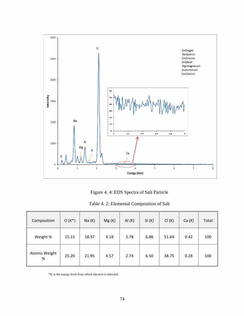
74
Figure 4. 4: EDS Spectra of Salt Particle
Table 4. 2: Elemental Composition of Salt
Composition O (K*) Na (K) Mg (K) Al (K) Si (K) Cl (K) Ca (K) Total
Weight % 15.15 18.97 4.18 2.78 6.86 51.64 0.42 100
Atomic Weight %
25.20 21.95 4.57 2.74 6.50 38.75 0.28 100
*K is the energy level from which electron is detected.

75
The XRD and SEM analysis substantiates the presence of chlorine as a major element in
salt, and presence of chlorine ion may significantly weaken the integrity of cement matrix (Berke
et al., 1988). For this reason, special consideration must be given to compensate the strength
including durability issues when salt is used as alternative construction material.
4.3 Fly Ash
The details of fly ash chemical proportion, crystalline properties, glassy composition and
physical properties were described in Section 2.2. Paya et al. (1996) documented the effect of
ignition, fineness, particle distribution, shape morphology, and smoothness of fly ash particles on
rheological behavior, flowability and workability of the mixture. Moreover, fly ash fineness and
mineralogy also influences strength of mortar or PCC. In this chapter, XRD and SEM analysis
results for Class-F fly ash samples is presented.
4.3.1 XRD Analysis
XRD pattern for fly ash sample is shown in Figure 4.5 which illustrates that the main
crystalline phases are quartz (JCPDS# 01-074-1811) and mullite (JCPDS# 01-088-2049). The
presence of large proportion of aluminosilicate glassy phase (mullite) in fly ash is primarily due
to rapid cooling at high temperature. Alumina to silica ratio of this mullite is 5:2. Mullite is
chemically inert in PCC or mortar ( ACI Committee 232, 1996). Beside these crystal phases, the
XRD pattern of fly ash indicates that the other crystalline phase present are Hematite (Fe2O3) and
Calcium Oxide (CaO). The patterns were matched with JCPDS #01-071-5088 and JCPDS# 01-
070-5490, respectively. In Figure 4.5, presence of quartz, mullite, hematite and calcium oxide
are represented by Q, M, H and CaO respectively. Very low intensity of calcium oxide in XRD
pattern validates insignificant presence of calcium in fly ash sample. According to ACI, presence
of quartz, hematite, and calcium oxide increases strength and improves durability of PCC.
Therefore, the gain in strength of mortar prepared with Class-F fly ash will be less and slow in
comparison to fly ash consisting of higher calcium oxide.
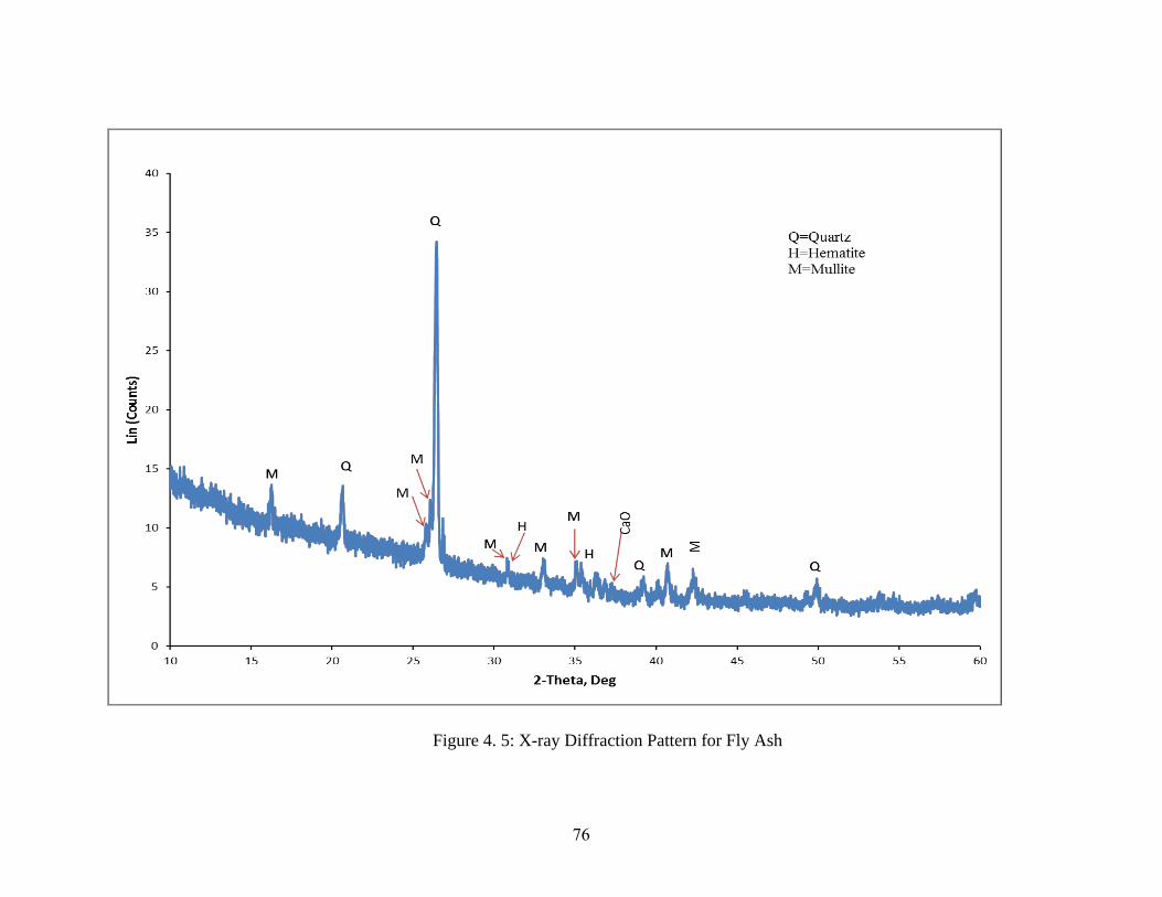
76
Figure 4. 5: X-ray Diffraction Pattern for Fly Ash
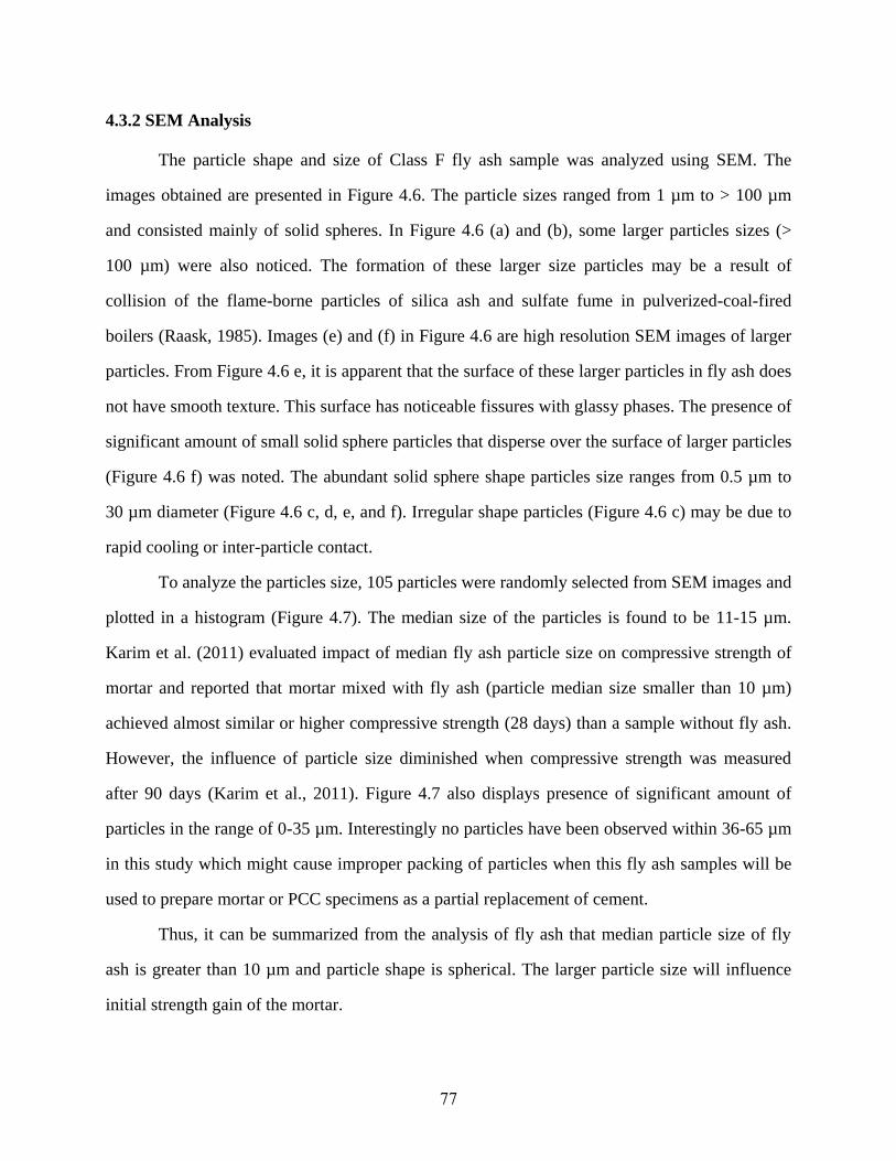
77
4.3.2 SEM Analysis
The particle shape and size of Class F fly ash sample was analyzed using SEM. The
images obtained are presented in Figure 4.6. The particle sizes ranged from 1 µm to > 100 µm
and consisted mainly of solid spheres. In Figure 4.6 (a) and (b), some larger particles sizes (>
100 µm) were also noticed. The formation of these larger size particles may be a result of
collision of the flame-borne particles of silica ash and sulfate fume in pulverized-coal-fired
boilers (Raask, 1985). Images (e) and (f) in Figure 4.6 are high resolution SEM images of larger
particles. From Figure 4.6 e, it is apparent that the surface of these larger particles in fly ash does
not have smooth texture. This surface has noticeable fissures with glassy phases. The presence of
significant amount of small solid sphere particles that disperse over the surface of larger particles
(Figure 4.6 f) was noted. The abundant solid sphere shape particles size ranges from 0.5 µm to
30 µm diameter (Figure 4.6 c, d, e, and f). Irregular shape particles (Figure 4.6 c) may be due to
rapid cooling or inter-particle contact.
To analyze the particles size, 105 particles were randomly selected from SEM images and
plotted in a histogram (Figure 4.7). The median size of the particles is found to be 11-15 µm.
Karim et al. (2011) evaluated impact of median fly ash particle size on compressive strength of
mortar and reported that mortar mixed with fly ash (particle median size smaller than 10 µm)
achieved almost similar or higher compressive strength (28 days) than a sample without fly ash.
However, the influence of particle size diminished when compressive strength was measured
after 90 days (Karim et al., 2011). Figure 4.7 also displays presence of significant amount of
particles in the range of 0-35 µm. Interestingly no particles have been observed within 36-65 µm
in this study which might cause improper packing of particles when this fly ash samples will be
used to prepare mortar or PCC specimens as a partial replacement of cement.
Thus, it can be summarized from the analysis of fly ash that median particle size of fly
ash is greater than 10 µm and particle shape is spherical. The larger particle size will influence
initial strength gain of the mortar.
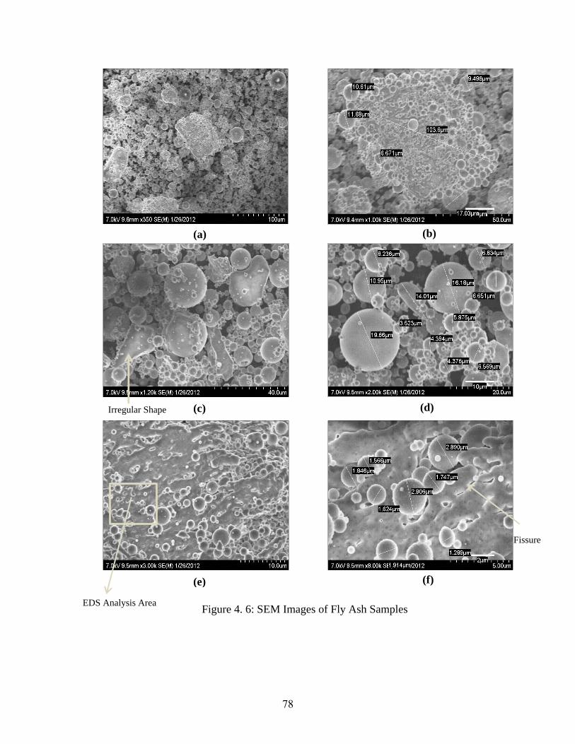
78
Figure 4. 6: SEM Images of Fly Ash Samples
(a) (b)
(c) (d)
(e) (f)
Fissure
EDS Analysis Area
Irregular Shape

79
Figure 4. 7: The Particle Size distribution of Fly Ash
4.3.3 EDS Analysis
The EDS curve obtained for fly ash sample is shown in Figure 4.8. The SEM images of
the sample and the area analyzed to obtain the EDS data are shown as insert in Figure 4.8. The
composition determined from EDS is presented in Table 4.3. It is evident that the predominant
elements of Class-F fly ash sample are aluminum (Al), silicon (Si) and oxygen (O). These
elements have showed most intense peaks in EDS spectra (Figure 4.8). The presence of Al and Si
indicates presence of quartz and mullite which is similar to the XRD analysis. Sodium (Na) was
observed as a minor element with major element aluminum and silicon. Also, presence of iron
(Fe) verifies existence of it as hematite was found during XRD analysis. Magnesium (Mg) sulfur
(S), potassium (K) and calcium (Ca) were identified as trace elements (% by wt. <1).
Magnesium, sulfur and potassium may exist with alumina and silica; however, calcium was
observed as calcium oxide compound present in the samples.
0
5
10
15
20
25
30
35
Fre
qu
en
cy
Size (µm)
80
Figure 4. 8: EDS Spectra of Fly Ash
Table 4. 3: Elemental Composition of Fly Ash
Composition O(K*) Na (K) Mg(K) Al (K) Si (K) S(K) K(K) Ca (K) Fe (K) Total
Weight % 39.47 1.57 0.52 24.7 30.11 0.38 0.51 0.91 1.82 100
Atomic weight %
53.35 1.47 0.46 2.74 23.18 0.25 0.28 0.49 0.70 100
*K is the energy level from which electron is detected.
EDS Analysis Area
81
4.4 Mortar
4.4.1 Compressive Strength Test
As stated in section 3.3, the compressive strength testing of in. cube specimens was
performed after 3, 7 and 28 days of curing. The average compressive strength was obtained from
average of three samples. The test results of compressive strength at different ages are
summarized in Figure 4.9 along with standard deviation error bar. Strength activity index (SAI)
and strength growth rate of different mortar specimens is shown in Figures 4.10 and Figure 4.11,
respectively. The mortar cubes prepared with cement, sand and sodium phosphate buffer (CSP
sample) were used as a control sample.
To understand the effect of sodium phosphate buffer, the strength of samples prepared
with normal tap water (CSW) and sodium phosphate buffer (CSP) was compared. From Figure
4.9, it is clear that CSP samples have 8.5 percent higher compressive strength than 3 day
compressive strength of CSW samples. This can be attributed to slightly higher pH 7.5 of
phosphate buffer which quickens the hydration reaction of cement. However, both samples
gained almost similar compressive strength after 28 days of curing (CSW sample: 5440 psi, CSP
sample: 5430 psi). So, it can be concluded that sodium phosphate buffer does not significantly
influence ultimate strength of samples except very early strength.
To identify optimum fly ash content, specimens were prepared by replacing 5, 10, 20 and
40 percent of cement with fly ash. It was noticed that increasing the amount of fly ash decreased
the compressive strength of specimens at all three ages in comparison to samples prepared
without fly ash (CSP or CSW). The sample CSFP5% prepared with 5 percent fly ash had 4.8
percent lower 28 day compressive strength (5170 psi) than sample without fly ash (CSP sample:
5430 psi). In case of 40 percent fly ash replacement, the 28 day strength of sample reduced by 25
percent than sample without fly ash (CSFP 40% sample: 4050 psi, CSP sample: 5430 psi).
Conventionally, addition of fly ash (Class-C fly ash) usually increases or at least provides
ultimate strength similar to mortar prepared without fly ash. However, the strength gain of PCC
or mortar also depends on size of fly ash particles and on its crystalline properties. From XRD

82
and SEM analysis of Class F fly ash, it had been found that this fly ash sample is predominant
with mullite, silica and alumina phase and median particle size is greater than 10 µm which
results in slower pozzolanic reaction. For this reason the specimens prepared with Class-F fly ash
partially replacing cement, gained lower 28 day compressive strength than control specimen
CSP.
From Figure 4.10, it is evident that SAI, which is a ratio in percentage between the
compressive strength of the mortar and control mortar at the same ages, is also lower for all
mortar cubes prepared with fly ash than control mortar cube CSP. It is also noticed that strength
gain rate from seven to twenty eight days, due to pozzolanic reaction of fly ash, is more when
more than 20 percent fly ash was added (Figure 4.11). The samples prepared with 40 percent
replacement of cement by fly ash has more than 50 % strength gain rate from 7 to 28 days,
highest among the samples prepared with cement, sand and fly ash. Only bacteria treated sample
has such strength gain rate, as explained in the following paragraphs.
Since addition of more than 5% fly ash did not improve compressive strength
significantly, remaining experiments were performed with replacement of cement with only 5
percent fly ash. Although there is loss of strength with addition of fly ash, the main advantage of
fly ash in this study is improvement in durability and optimum environment for growth of
bacteria.
The optical density (a measurement of bacteria concentration) was kept constant at 0.6
for all bacteria treated sample and the ratio between cementitious materials to sodium phosphate
buffer was kept constant at 0.485. The high alkaline pH of PCC as well as addition of salts
influence the optimum environment for bacteria growth, hence, mutated B. pasteurii bacteria was
only used to prepare specimens with salt.

83
Figure 4. 9: Strength of Different Type of Mortar Specimens
CSW CSP CSSP 5% CSFP 5%CSSFP
5%CSFB5%
CSMBCSFMB
5%CSSFMB
5%CSFP10%
CSFP20%
CSFP30%
CSFP40%
3 Day strength 4140 4500 2730 4180 2640 3760 3570 3580 3040 3770 2960 2610 2370
7 day Strength 4560 4750 3200 4380 3340 4460 3850 4090 3850 4270 3680 3070 2670
28 Day Strength 5440 5430 3500 5170 4430 6170 5630 6200 4640 4770 4410 4130 4050
0
1000
2000
3000
4000
5000
6000
7000
Com
pre
ssiv
e S
tren
gth
(P
si)
C: Cement S:Sand S:Salt F:Fly Ash P: Sodium Phosphate Buffer B:Normal Bacteria with buffer MB:Mutated Bacteria with buffer

84
Figure 4. 10: Strength Activity Index of Mortar Specimens
CSW CSPCSSP5%
CSFP5%
CSSFP5%
CSFB5%
CSMBCSFMB
5%CSSFMB 5%
CSFP10%
CSFP20%
CSFP30%
CSFP40%
3 Day Strength Activity Index 92 100 61 93 59 84 79 80 68 84 66 58 53
7 Day Strength Activity Index 96 100 67 92 70 94 81 86 81 90 77 65 56
28 Day Strength Activity Index 100 100 64 95 82 114 104 114 85 88 81 76 75
0
20
40
60
80
100
120
Str
enn
gth
Act
ivit
y I
nd
ex (
%)
C: Cement S: Sand S:Salt P: Sodium phosphate Buffer F:Fly Ash B: Normal Bacteria with Buffer MB: Mutated Bacteria with Buffer
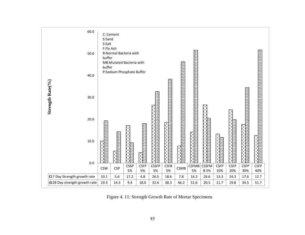
85
Figure 4. 11: Strength Growth Rate of Mortar Specimens
CSW CSPCSSP5%
CSFP5%
CSSFP5%
CSFB5%
CSMBCSFMB
5%CSSFMB 5%
CSFP10%
CSFP20%
CSFP30%
CSFP40%
7 Day Strength growth rate 10.1 5.6 17.2 4.8 26.5 18.6 7.8 14.2 26.6 13.3 24.3 17.6 12.7
28 Day strength growth rate 19.3 14.3 9.4 18.0 32.6 38.3 46.2 51.6 20.5 11.7 19.8 34.5 51.7
0.0
10.0
20.0
30.0
40.0
50.0
60.0
Str
ength
Rate
(%)
C: Cement S:Sand S:Salt F:Fly Ash B:Normal Bacteria with buffer MB:Mutated Bacteria with buffer P:Sodium Phosphate Buffer

86
Initially addition of salt impact was investigated. From Figure 4.9, observing the strength
of samples CSP, CSSP5% and CSSFP5% at different ages, it is clear that addition of salt
considerably reduced the strength at all ages than control sample CSP. Berke et al. (1988)
reported that chloride ions presence in solution may weaken the integrity of cement matrix. It is
also discerned that addition of salt slows the hydration reaction by about 5% (Strength growth
rate from 7-28 days, CSP sample =14.3%, CSSP5% sample =9.4%, Figure 4.11). However, use
of fly ash (5 percent) in presence of salt (CSSFP5%) not only improved the ultimate strength
(4430 psi) in comparison to samples prepared with salt (CSSP5% = 3500 psi) but CSSFP5%
sample also gained strength at higher rate from 7-28 days. It substantiates that this salt might not
have any effect on pozzolanic reaction or increase the rate of pozzolanic reaction when used with
fly ash. Moreover, Figure 4.11 showed that SAI value is 82 percent at 28 day of CSSFP5%
sample which is far better than CSSP5% sample (SAI =64%). Thus, it can be concluded that
addition of fly ash with salt increases the compressive strength of mortar specimens but not to
the levels observed with control specimens.
The specimens treated with bacteria performed better with respect to compressive
strength. Samples prepared with fly ash and normal bacteria (CSFB5%) and fly ash with mutated
bacteria (CSFMB5%) achieved 6170 psi and 6200 psi compressive strength after 28 days of
curing, respectively. It is maximum compressive strength attained among all of the tested
samples. This strength is almost more than 14 percent in comparison to control sample (CSP).
The fly ash with mutated bacteria (CSFMB5%) samples gained 570 psi more (28 day
compressive strength) than samples prepared with mutated bacteria only (CSMB: 5630 psi).
From Figure 4.11, it was also noticed that the strength gain rate from 7-28 days for CSMB5%
and CSFMB5% samples are 46 % and 52%, respectively. This information verifies that the
strength improvement primarily occurs due to calcite precipitation by bacteria in these samples.
According to Lane et al. (1982), the fly ash with median particle size lager than 10 µm
and more inactive mullite phase is mixed with specimen causes slower pozzolanic reaction that

87
hinders strength gain. So, a comparison study was done between CSFP5%, CSSFP5%,
CSFMB5%, CSSFMB5% samples and is presented in Table 4.4.
Table 4. 4: Comparison between CSFP5%, CSSFP5%, CSFMB5% and CSSFMB5%
Table 4.4 shows that addition of fly ash and mutated bacteria to mortar has increased 28
day compressive strength than mortar containing only fly ash. Besides this, mutated bacteria with
fly ash amended mortar sample (CSFMB5%) not only has highest strength gain rate from 7- 28
days more than 50 percent as like the sample CSFP 40% , the sample prepared by 40% fly ash
replacement; but also it has maximum strength activity index (SAI) = 114%. Likewise,
CSSFMB5% sample achieved more strength than CSSFP5% sample. But the compressive
strength of CSSFMB5% did not increase significantly as with CSFMB5% sample that might be
due to premature death of mutated bacteria cell or formation of endospore at higher alkaline pH
in concrete environment with salt.
Verenyam Achal et al. (2011) suggested that bacteria have a better survival rate in the
presence of fly ash because fly ash creates finer pores to get better aeration, which is required for
Sample
28 day
Compressive
Strength (Psi)
Strength Gain Rate
(%) from 7 to 28
day
Strength Activity
Index (SAI, %)
with respect to
CSP sample for 28
Day Strength
CSFP5% 5170 18 95
CSSFP5% 4430 32.6 82
CSFMB5% 6200 51.6 114
CSSFMB5% 4640 20.5 85

88
better growth. Furthermore, the dead cells in the mortar cement matrix act as organic fiber to
increase the compressive strength of the cube (Ramachandran et al., 2001). It implies that when
bacteria are used with fly ash, the microbial activity improves the compressive strength by
precipitating calcite on cell surfaces as well as within the cement fly ash matrix, and this biotic
activity also induces pozzolanic reaction rate to increase strength at later ages.
From the above discussion, the following summary can be drawn:
Sodium phosphate buffer has an insignificant influence on compressive strength.
Use of salt as a partial replacement of sand can lower the ultimate compressive
strength of mortar or PCC.
Use of fly ash along with MB can recuperate loss of compressive strength of
mortar when salt is used as replacement of sand.
The mortar prepared with fly ash and MB exhibited maximum ultimate
compressive strength.
4.4.2 Freeze Thaw Test
As mentioned in Section 3.4.1, the 2 in. cube samples were evaluated for freeze thaw test.
The purpose of this experiment is to determine the loss of particles from specimens to evaluate
the resistance due to change in environment. The samples were subjected to two different
continuous cycles of freezing and thawing for 24 hr each. The test is continued for 28 days. The
durability factor is computed in accordance with the procedure specified in ASTM C 1645M-09.
The total mortar loss at 7 days and 28 days is the only quantifiable durability factor for this test.
Each freezing cycles was maintained at -5ºC and thawing cycle temperature was maintained at 5
ºC. The detailed procedure and collection of loss particles is describe in Section 3.3.1. The
average of three samples was taken as mortar loss at specific ages. Figure 4.12 shows the mortar
loss (g/m2) data in a column chart for 7 day and 28 day, respectively.
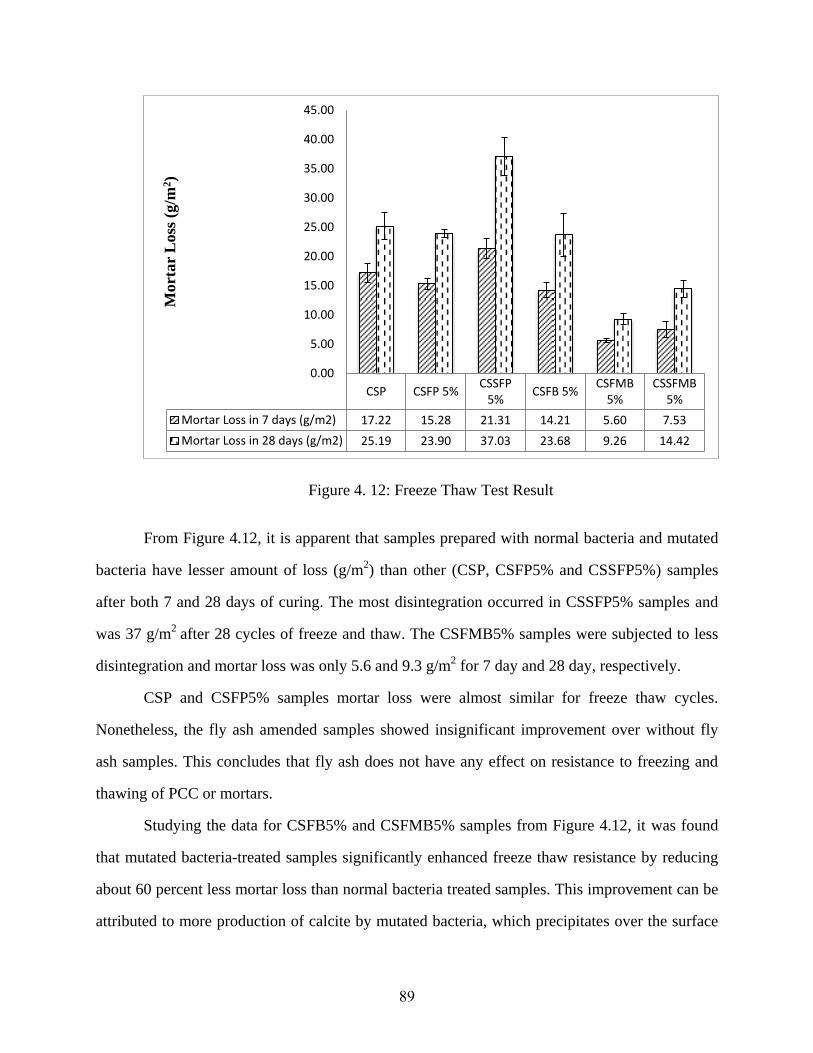
89
Figure 4. 12: Freeze Thaw Test Result
From Figure 4.12, it is apparent that samples prepared with normal bacteria and mutated
bacteria have lesser amount of loss (g/m2) than other (CSP, CSFP5% and CSSFP5%) samples
after both 7 and 28 days of curing. The most disintegration occurred in CSSFP5% samples and
was 37 g/m2
after 28 cycles of freeze and thaw. The CSFMB5% samples were subjected to less
disintegration and mortar loss was only 5.6 and 9.3 g/m2 for 7 day and 28 day, respectively.
CSP and CSFP5% samples mortar loss were almost similar for freeze thaw cycles.
Nonetheless, the fly ash amended samples showed insignificant improvement over without fly
ash samples. This concludes that fly ash does not have any effect on resistance to freezing and
thawing of PCC or mortars.
Studying the data for CSFB5% and CSFMB5% samples from Figure 4.12, it was found
that mutated bacteria-treated samples significantly enhanced freeze thaw resistance by reducing
about 60 percent less mortar loss than normal bacteria treated samples. This improvement can be
attributed to more production of calcite by mutated bacteria, which precipitates over the surface
CSP CSFP 5%CSSFP
5%CSFB 5%
CSFMB5%
CSSFMB5%
Mortar Loss in 7 days (g/m2) 17.22 15.28 21.31 14.21 5.60 7.53
Mortar Loss in 28 days (g/m2) 25.19 23.90 37.03 23.68 9.26 14.42
0.00
5.00
10.00
15.00
20.00
25.00
30.00
35.00
40.00
45.00
Mort
ar
Loss
(g/m
2)
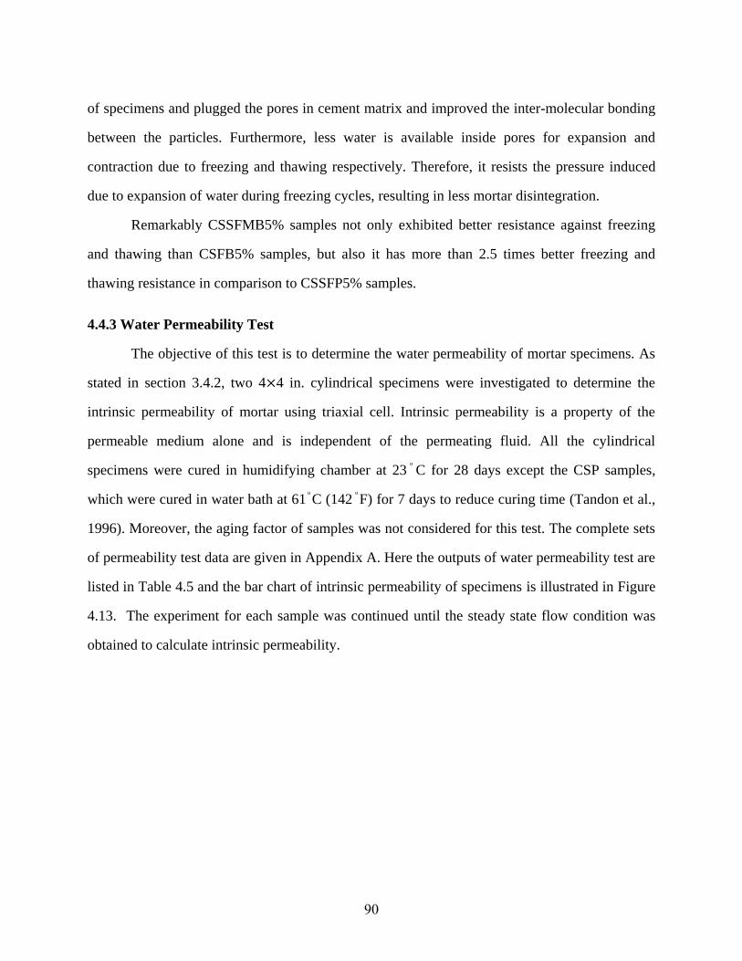
90
of specimens and plugged the pores in cement matrix and improved the inter-molecular bonding
between the particles. Furthermore, less water is available inside pores for expansion and
contraction due to freezing and thawing respectively. Therefore, it resists the pressure induced
due to expansion of water during freezing cycles, resulting in less mortar disintegration.
Remarkably CSSFMB5% samples not only exhibited better resistance against freezing
and thawing than CSFB5% samples, but also it has more than 2.5 times better freezing and
thawing resistance in comparison to CSSFP5% samples.
4.4.3 Water Permeability Test
The objective of this test is to determine the water permeability of mortar specimens. As
stated in section 3.4.2, two 4 4 in. cylindrical specimens were investigated to determine the
intrinsic permeability of mortar using triaxial cell. Intrinsic permeability is a property of the
permeable medium alone and is independent of the permeating fluid. All the cylindrical
specimens were cured in humidifying chamber at 23
C for 28 days except the CSP samples,
which were cured in water bath at 61 C (142
F) for 7 days to reduce curing time (Tandon et al.,
1996). Moreover, the aging factor of samples was not considered for this test. The complete sets
of permeability test data are given in Appendix A. Here the outputs of water permeability test are
listed in Table 4.5 and the bar chart of intrinsic permeability of specimens is illustrated in Figure
4.13. The experiment for each sample was continued until the steady state flow condition was
obtained to calculate intrinsic permeability.

91
Table 4. 5: Output of Water Permeability Test
Sample Age at the
time of testing (days)
Saturated Surface Wt. (g)
Dry Wt. (g) Porosity (%) Intrinsic
Permeability (m2)
Coefficient of Permeability (m/s)
CSP 1 7 1651.10 1449.00 25 8.56E-12 9.00E-06
CSP 2 7 1625.10 1415.00 26 1.01E-11 1.06E-05
CSFP5% 1 48 1677.30 1490.60 22 6.97E-12 7.32E-06
CSFP5% 2 48 1670.00 1490.60 22 6.09E-12 6.40E-06
CSSFP5% 1 53 1592.00 1373.40 27 2.57E-11 2.70E-05
CSSFP5% 2 53 1638.00 1404.00 28 2.08E-11 2.18E-05
CSFB5% 1 58 1612.60 1394.80 26 8.68E-12 9.12E-06
CSFB5% 2 - - - - - -
CSFMB5% 1 62 1574.80 1365.90 25 7.42E-12 7.80E-06
CSFMB5% 2 60 1596.20 1370.80 27 7.88E-12 8.28E-06
CSSFMB5% 1 60 1648.30 1461.50 23 4.63E-12 4.87E-06
CSSFMB5% 2 60 1653.60 1453.40 24 3.22E-12 3.39E-06

92
Figure 4. 13: Intrinsic Permeability (m2) of Specimens
From Table 4.5 and Figure 4.13, it had been found that the maximum average intrinsic
permeability was m2 for CSSFP5% sample among all the samples. As these
CSSFP5% samples were cured in water, salt leached out from the specimens, creating a larger
pore size. Nevertheless, salt may weaken the cement matrix integrity, causing poor pore
connectivity. For these reasons, the samples with salt and fly ash have higher permeability as
well as porosity.
The fly ash amended samples CSFP5% had 1.4 times lower permeability than
sample prepared without fly ash (CSP). This is primarily due to formation of C-S-H adhesive gel
by pozzolanic activity in fly ash sample, which might refines the pore network of concrete and
make mortar less permeable.
CSP CSFP CSSFP CSFB CSFMB CSSFMB
Sample 1 8.56E-12 6.97E-12 2.57E-11 8.68E-12 7.42E-12 4.63E-12
Sample 2 1.01E-11 6.09E-12 2.08E-11 0.00E+00 7.88E-12 3.22E-12
0.00E+00
5.00E-12
1.00E-11
1.50E-11
2.00E-11
2.50E-11
3.00E-11
Intr
insi
c P
erm
eab
ilit
y (
m2)

93
Permeability results of samples prepared with mutated bacteria CSFMB5% and normal
bacteria CSFB5% have showed almost similar improvement like the samples prepared with fly
ash CSFP5%. CSFMB5% samples were 13 percent less permeable than CSFB5% samples. This
can be easily explained as mutated bacteria precipitate more calcite over the surface and between
pores. Thus, it reduces the pores size and improves the pore connectivity by creation of tortuous
network to lower the permeability.
These principles also hold true for CSFMB5% samples prepared with mutated bacteria,
fly ash and salts. This sample has lowest permeability and about 6 times less permeable than
CSSFP5%. Additionally, lesser porosity (%) of CSSFMB5% than CSSFP5% sample also
validates filling up of pores and, or refinement of pore connectivity with microbial calcite
precipitation.
So, it can be recapitulates from the above discussion that not only fly ash addition lowers
the permeability from control samples but the use of microorganisms further reduces the
permeability by creating a more tortuous pore network and by filling the pores with calcium
carbonate precipitate to make pores completely filled or narrower.
However, Neithalath et al. (2006) showed that permeability is not a function of porosity
and pore size alone, rather it depends on complex pore connectivity too. Furthermore, a more
scrutinized experiment is required to better predict permeability to pore system of mortar or
concrete specimens with the help of micro-level testing such as scanning electron microscope.
4.4.4 Absorption Test
The absorption test is performed on 2 in. mortar cube as per procedure illustrated in
Section 3.4.3. The main objective of this test is to find out the initial absorption rate (%) for first
6 hr. The secondary absorption rate was not determined as correlation coefficient was less than
0.98 which is required as per ASTM C1585-11. In addition to the procedure, electrical
conductivity and pH readings were collected at different intervals followed by an ion
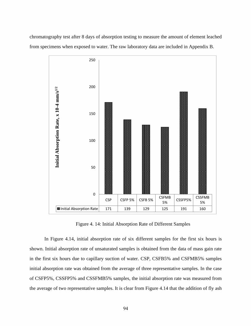
94
chromatography test after 8 days of absorption testing to measure the amount of element leached
from specimens when exposed to water. The raw laboratory data are included in Appendix B.
Figure 4. 14: Initial Absorption Rate of Different Samples
In Figure 4.14, initial absorption rate of six different samples for the first six hours is
shown. Initial absorption rate of unsaturated samples is obtained from the data of mass gain rate
in the first six hours due to capillary suction of water. CSP, CSFB5% and CSFMB5% samples
initial absorption rate was obtained from the average of three representative samples. In the case
of CSFP5%, CSSFP5% and CSSFMB5% samples, the initial absorption rate was measured from
the average of two representative samples. It is clear from Figure 4.14 that the addition of fly ash
CSP CSFP 5% CSFB 5%CSFMB
5%CSSFP5%
CSSFMB5%
Initial Absorption Rate 171 139 129 125 191 160
0
50
100
150
200
250In
itia
l A
bso
rpti
on
Rate
, x 1
0-4
mm
/s1
/2

95
in mortar sample CSFP5% had a 23 percent lower initial absorption rate than without fly ash
sample (CSP). Since fly ash reduced porosity by producing C-S-H gel, this activity led to
subsequent refinement of pores by decreasing size or plugging it. Therefore, CSFP5% sample
had less capillary suction than CSP sample.
Also, it was observed that bacteria and fly ash amended samples CSFB5% and
CSFMB5% had lower initial absorption rate than all others samples, as microbial activity of
calcite consolidation enhance fly ash effectiveness in mortar specimens by plugging the pores.
So, the deposition of calcite by microbial activity can seal voids, pores and cracks of microscopic
size where other sealant cannot go. Both CSFB5% and CSFMB5% have almost similar
absorption rate and they are 129 × 〖10〗^(- ) mm/√sec and 12 × 〖10〗^(- ) mm/√sec,
respectively. This initial absorption rate of CSFB5% and CSFMB5% samples is almost 9.0 %
lower than fly ash amended CSFP5% sample.
The highest initial absorption rate obtained for CSSFP5% was 191 × 〖10〗^(-4)
mm/√sec sample. Because leaching of salt elements during curing period turned mortar
specimens more porous, yielding more capillary suction rate for CSSFP5% samples. On the
other hand, the sample CSSFMB5% prepared with salt, fly ash and mutated bacteria showed 19
percent lower absorption rate than CSSFP5% sample, as bacterial calcite precipitation plugged
the pores in mortar specimen to minimize capillary suction.
In Figure 4.15, water absorption rate to sample mass ratio was plotted for the first 6 hr.
The initial absorption rate of a specific sample was used to calculate water absorption amount for
a specific time and then it was divided by the sample mass to get the ratio. Water absorption
amount for specific time was not used directly, as samples initial masses were different. Figure
4.15 show that CSSFP5% sample is absorbing more water than any other samples. CSFB5%,
CSFMB5%, CSP, and CSSFMB5% samples have almost similar absorption pattern for first six
hour. So considering absorption characteristics, it capitulates that mutated bacteria and fly ash
are able to better stabilize salt added samples to make it less durable similar to samples prepared
with cement and sand.
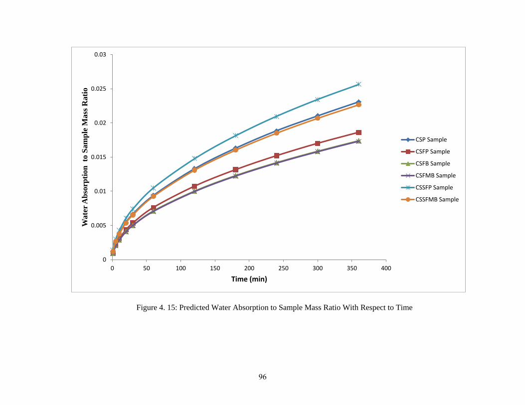
96
Figure 4. 15: Predicted Water Absorption to Sample Mass Ratio With Respect to Time
0
0.005
0.01
0.015
0.02
0.025
0.03
0 50 100 150 200 250 300 350 400
Wate
r A
bso
rpti
on
to
Sam
ple
Mass
Rati
o
Time (min)
CSP Sample
CSFP Sample
CSFB Sample
CSFMB Sample
CSSFP Sample
CSSFMB Sample

97
4.4.4.1 Discussion on Ion Chromatography Test Result
Ion chromatography (IC) test was performed mainly to measure the concentration of ions
in de-ionized water which leached from samples during the absorption test. The IC test was
performed after performing absorption tests for eight days. The pH and Electrical conductivity
readings were taken using “Pool Pro” device, manufactured by Myron L Company. This device
was calibrated using standard solution before taking readings of water. IC test quantitatively
measured the amount of ion (mg/l) present in de-ionized water. To better interpret the data, ion
mg. per liter of de-ionized water was converted to ion leached mg. per gram of sample. From IC
test results, the ions identified in de-ionized water are presented in Figures 4.16 through 4.18.
The average amount of sodium and calcium ions leached from CSP and CSFP5%
samples is less than 0.05 mg/g. The average amount of chlorine ion is significantly lower than
sodium and calcium, since there is no viable source of chlorine. The presence of sodium and
calcium can be attributed to use of SPB.
CSSFP5% sample had leached higher amount of sodium and chlorine than CSP and
CSFP5%. Salt (contains sodium, chloride ions) disintegrating cement matrix, this can be
attributed dissolving in water during curing period.
The bacteria treated samples CSFB5% and CSFMB5% had slightly more leaching of
sodium and chloride ions than CSP and CSFP5% samples (Figure 4.16 and 4.17). Urea calcium
chloride medium ingredients are nutrient broth for bacteria, urea, sodium bicarbonate,
ammonium chloride and calcium chloride. So, presence of sodium and chloride ions in CSFB5%
and CSFMB5% were partly contributed by the medium used for curing. It is conspicuous from
Figure 4.18 that CSFB5% and CSFMB5% have highest calcium leaching among all of the
samples. It is known that addition of fly ash reduces leaching of calcium in CSFP5% samples;
also the biologically consolidated calcium carbonate on mortar is insoluble in water, so source of

98
Figure 4. 16: Amount of Sodium (mg/g) Leached from Samples After 8 Days of Absorption
CSP CSFP 5% CSFB 5% CSFMB 5% CSSFP 5% CSSFMB 5%
Sample 1 0.024 0.042 0.044 0.037 0.495 0.658
Sample 2 0.038 0.024 0.041 0.028 0.466 0.570
Sample 3 0.044 0.025 0.036 0.046 0.464
0.000
0.200
0.400
0.600
0.800
1.000
1.200
Lea
chin
g A
mou
nt
(mg/g
)
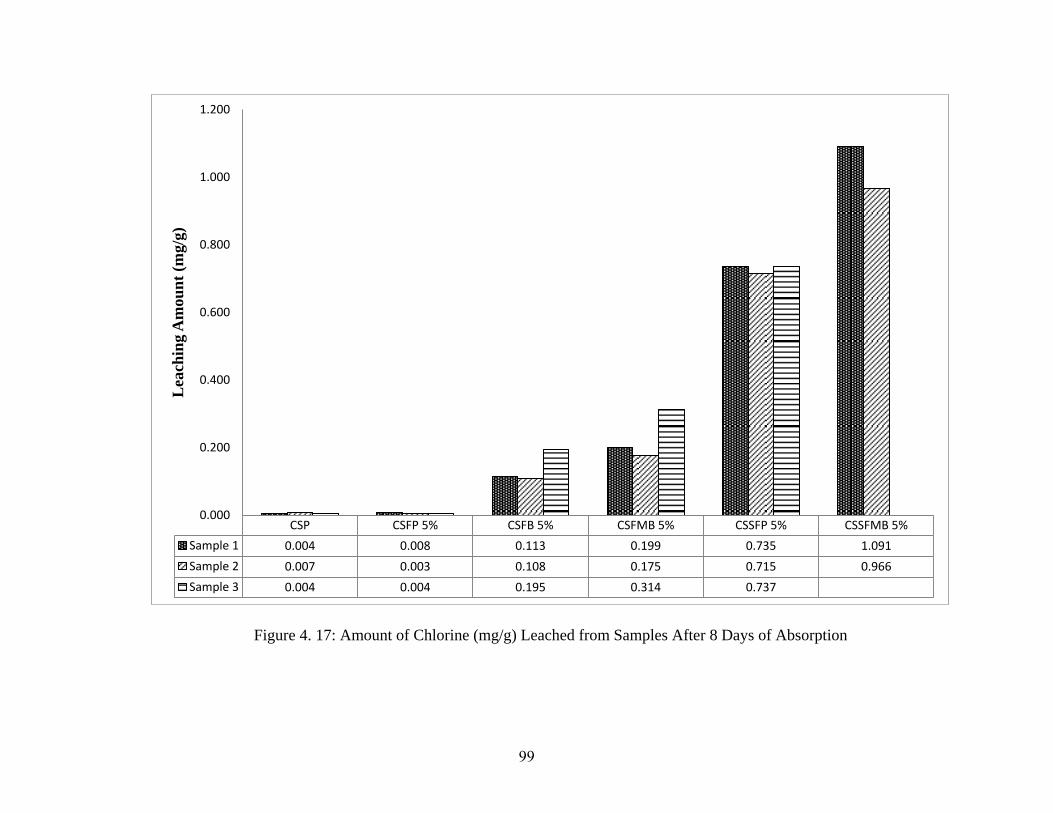
99
Figure 4. 17: Amount of Chlorine (mg/g) Leached from Samples After 8 Days of Absorption
CSP CSFP 5% CSFB 5% CSFMB 5% CSSFP 5% CSSFMB 5%
Sample 1 0.004 0.008 0.113 0.199 0.735 1.091
Sample 2 0.007 0.003 0.108 0.175 0.715 0.966
Sample 3 0.004 0.004 0.195 0.314 0.737
0.000
0.200
0.400
0.600
0.800
1.000
1.200
Lea
chin
g A
mou
nt
(mg/g
)

100
Figure 4. 18: Amount of Calcium (mg/g) Leached from Samples After 8 Days of Absorption
CSP CSFP 5% CSFB 5% CSFMB 5% CSSFP 5% CSSFMB 5%
Sample 1 0.020 0.006 0.048 0.074 0.020 0.030
Sample 2 0.018 0.012 0.054 0.093 0.024 0.035
Sample 3 0.008 0.013 0.101 0.122 0.033
0.000
0.200
0.400
0.600
0.800
1.000
1.200
Lea
chin
g A
mou
nt
(mg/g
)
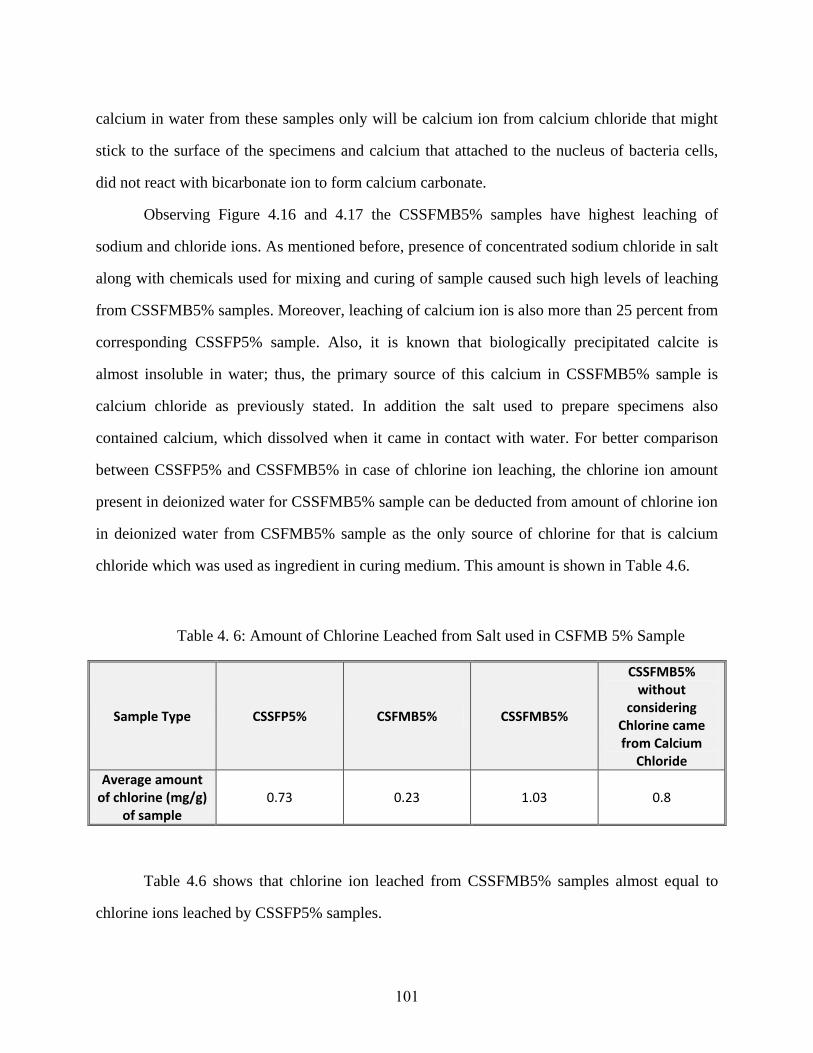
101
calcium in water from these samples only will be calcium ion from calcium chloride that might
stick to the surface of the specimens and calcium that attached to the nucleus of bacteria cells,
did not react with bicarbonate ion to form calcium carbonate.
Observing Figure 4.16 and 4.17 the CSSFMB5% samples have highest leaching of
sodium and chloride ions. As mentioned before, presence of concentrated sodium chloride in salt
along with chemicals used for mixing and curing of sample caused such high levels of leaching
from CSSFMB5% samples. Moreover, leaching of calcium ion is also more than 25 percent from
corresponding CSSFP5% sample. Also, it is known that biologically precipitated calcite is
almost insoluble in water; thus, the primary source of this calcium in CSSFMB5% sample is
calcium chloride as previously stated. In addition the salt used to prepare specimens also
contained calcium, which dissolved when it came in contact with water. For better comparison
between CSSFP5% and CSSFMB5% in case of chlorine ion leaching, the chlorine ion amount
present in deionized water for CSSFMB5% sample can be deducted from amount of chlorine ion
in deionized water from CSFMB5% sample as the only source of chlorine for that is calcium
chloride which was used as ingredient in curing medium. This amount is shown in Table 4.6.
Table 4. 6: Amount of Chlorine Leached from Salt used in CSFMB 5% Sample
Sample Type CSSFP5% CSFMB5% CSSFMB5%
CSSFMB5% without
considering Chlorine came from Calcium
Chloride
Average amount of chlorine (mg/g)
of sample 0.73 0.23 1.03 0.8
Table 4.6 shows that chlorine ion leached from CSSFMB5% samples almost equal to
chlorine ions leached by CSSFP5% samples.

102
pH readings of water also measured after eight days of absorption to check the effect of
elements leached in water from samples. Figure 4.19 shows the pH reading of the samples after
completion of test. The initial pH of de-ionized water was 7.10. There is insignificant difference
of pH among CSP, CSFP5% and CSSFP5% samples water. The average pH of CSP and
CSFP5% water samples were 9.7 and 9.5. CSFP5% water samples had slightly lower pH as it
leached less calcium hydroxide (Ca(OH)2). The higher pH of CSSFP5% sample is mainly due to
leaching of freer Ca(OH)2 from samples.
However, the prominent result is bacteria treated water samples have lower pH (range 7.0
to 8.5). This can be explained by two reasons. Firstly, the bacteria inside mortar specimens can
produce ammonia (NH3) using urea present in sample by biotic activity, and NH3 can react with
H+ ion to produce acidic NH4
+ ion to neutralize pH. Another reason is presence of ammonium
chloride and sodium bicarbonate chemicals as curing medium ingredients, may stick to the
bacteria treated samples. So when these chemicals come in contact with water may form
ammonium, bicarbonate ion to reduce pH of the media. For similar reasons, CSSFMB5% water
samples had slightly decrease pH than CSP, CSFP5% and CSSFP5% samples.
From above discussion, it is clear that the main reason for drop of pH for bacteria treated
sample is still requires further investigation. In fact, if it holds true then bacteria treated sample
can be used in large underwater or underground construction as it does not affect the pH of
water.
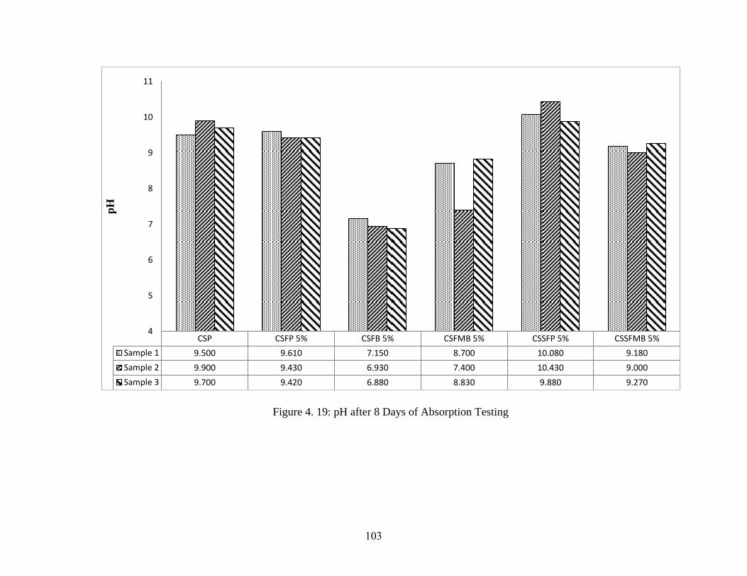
103
Figure 4. 19: pH after 8 Days of Absorption Testing
CSP CSFP 5% CSFB 5% CSFMB 5% CSSFP 5% CSSFMB 5%
Sample 1 9.500 9.610 7.150 8.700 10.080 9.180
Sample 2 9.900 9.430 6.930 7.400 10.430 9.000
Sample 3 9.700 9.420 6.880 8.830 9.880 9.270
4
5
6
7
8
9
10
11
pH
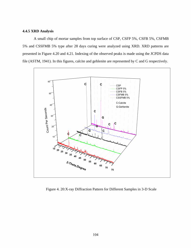
104
4.4.5 XRD Analysis
A small chip of mortar samples from top surface of CSP, CSFP 5%, CSFB 5%, CSFMB
5% and CSSFMB 5% type after 28 days curing were analyzed using XRD. XRD patterns are
presented in Figure 4.20 and 4.21. Indexing of the observed peaks is made using the JCPDS data
file (ASTM, 1941). In this figures, calcite and gehlenite are represented by C and G respectively.
1520
2530
3540
4550
5560
6570
75
0
10
20
30
40
50
60
CSP
CSFP 5%
CSFB 5%
CSFMB 5%
CSSFMB 5%
Count
Per
Seconds
2-Theta,Degree
C
C
C
G
G
G
CCC
CC
C:Calcite
G:Gehlenite
Figure 4. 20:X-ray Diffraction Pattern for Different Samples in 3-D Scale

105
Figure 4.21 depicts the profiles of XRD patterns of five different samples. The most
intense peak observed corresponds to the rhombohedral calcite (CaCO3). The peak position is at
2θ=29.16 , 29. 129, 29.3938, 29.38 3 and 29.330 degree for CSP, CSFP %, CSFB %,
CSFMB 5% and CSSMB 5%, respectively. This peak corresponds to XRD occurred from (104)
plane. The others most of the peaks were marked as calcite and all the bacteria treated samples
had exhibited more calcite peaks than CSP or CSFP 5% samples. Besides this, a noticeable peak
of Gelhenite (Ca2Al(AlSiO7)) was found at 2θ= 31. 33, 31. 0 1, 31.3 1 degree respectively
for CSFB 5%, CSFMB 5% and CSSFMB 5% samples. This peak was completely absent in CSP
and CSFP 5% samples. This suggests that microbial activity induce a new silicate phase
formation (gehlenite) within mortar matrix refine which the pore size distribution and improve
the compressive strength of bacteria treated specimens (Ghosh et al, 2005).
20 22 24 26 28 30 32 34 36 38 40
CP
S
2-Theta, Degree
CSSFMB
CSFMB
CSFB
CSFP
CSP
Calcite
Gehlenite
Figure 4. 21: X-ray iffraction Pattern of Samples from 20 to 0
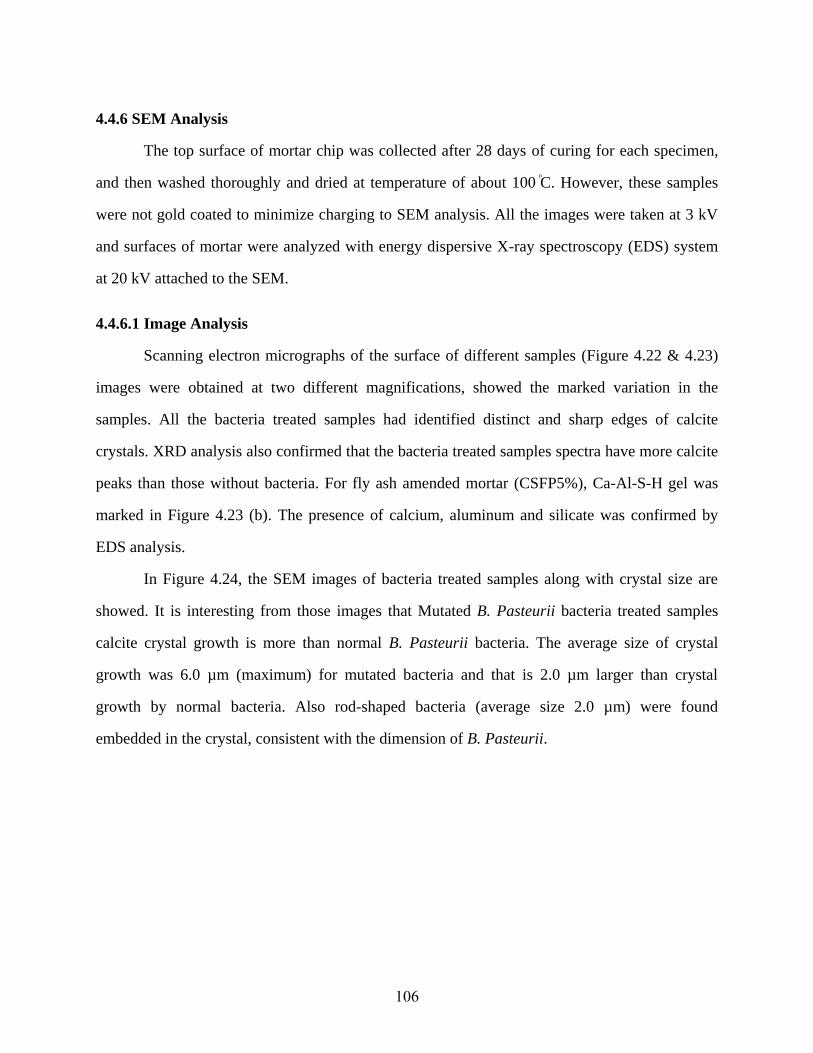
106
4.4.6 SEM Analysis
The top surface of mortar chip was collected after 28 days of curing for each specimen,
and then washed thoroughly and dried at temperature of about 100 C. However, these samples
were not gold coated to minimize charging to SEM analysis. All the images were taken at 3 kV
and surfaces of mortar were analyzed with energy dispersive X-ray spectroscopy (EDS) system
at 20 kV attached to the SEM.
4.4.6.1 Image Analysis
Scanning electron micrographs of the surface of different samples (Figure 4.22 & 4.23)
images were obtained at two different magnifications, showed the marked variation in the
samples. All the bacteria treated samples had identified distinct and sharp edges of calcite
crystals. XRD analysis also confirmed that the bacteria treated samples spectra have more calcite
peaks than those without bacteria. For fly ash amended mortar (CSFP5%), Ca-Al-S-H gel was
marked in Figure 4.23 (b). The presence of calcium, aluminum and silicate was confirmed by
EDS analysis.
In Figure 4.24, the SEM images of bacteria treated samples along with crystal size are
showed. It is interesting from those images that Mutated B. Pasteurii bacteria treated samples
calcite crystal growth is more than normal B. Pasteurii bacteria. The average size of crystal
growth was 6.0 µm (maximum) for mutated bacteria and that is 2.0 µm larger than crystal
growth by normal bacteria. Also rod-shaped bacteria (average size 2.0 µm) were found
embedded in the crystal, consistent with the dimension of B. Pasteurii.
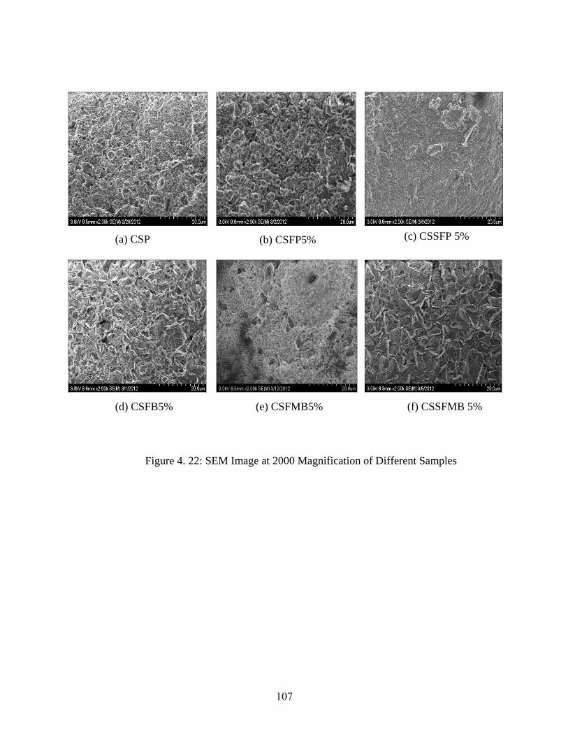
107
Figure 4. 22: SEM Image at 2000 Magnification of Different Samples
(a) CSP (b) CSFP5% (c) CSSFP 5%
(d) CSFB5% (e) CSFMB5% (f) CSSFMB 5%
108
Figure 4. 23: SEM Image at 8000 Magnification of Different Samples
(a) CSP (b) CSFP 5% (c) CSSFP 5%
(e) CSFMB5% (f) CSSFMB5% (d) CSFB5%
Ca-Al-S-H gel
(b) CSFP5%

109
Figure 4. 24: SEM Image with Bacteria and Crystal size
(a) CSFB 5%
(b) CSFMB 5%
(c) CSSFMB 5%
Spot Analysis
Point
Rod Shaped
Bacteria
Rod Shaped
Bacteria

110
4.4.6.2 Elemental Analysis
The elements present in the top surface of the samples were analyzed by EDS. The major
elements (wt. % > 10) are calcium (Ca), carbon (C) and oxygen (O). The other elements detected
are aluminum (Al), silicon (Si), chlorine (Cl), potassium (K) and magnesium (Mg). As Ca is the
main element that was discussed throughout this study, the concentration of this element for
different samples is presented in Table 4.7.
Table 4. 7: Elemental Analysis Result of Different Samples
Sample Type Calcium Amount (in %)
By Weight By Atomic weight
CSP 36.46 17.83
CSFP5% 33.99 16.01
CSSFP5% 28.60 13.14
CSFB5% 48.22 25.35
CSFMB5% 67.19 44.30
CSSFMB5% 43.60 22.24
From table 4.5 after observing the Ca wt. % of bacteria samples, it is substantiated that
bacterial activity consolidates calcium over the surface and pores of samples yield increase of the
weight by percentage of calcium. The maximum calcium precipitation (67% by wt.) occurs in
mutated bacteria treated samples. Calcium precipitation for normal bacteria is 19% less than
mutated bacteria. The use of mutated bacteria in salt added samples (CSSFMB5%) improved the
calcium consolidation over the surface and it is almost 15 percent greater than CSSFP5%
samples. The lowest amount of calcium was found in CSSFP5% samples which also validated
that addition of salt disintegrates the cement matrix.
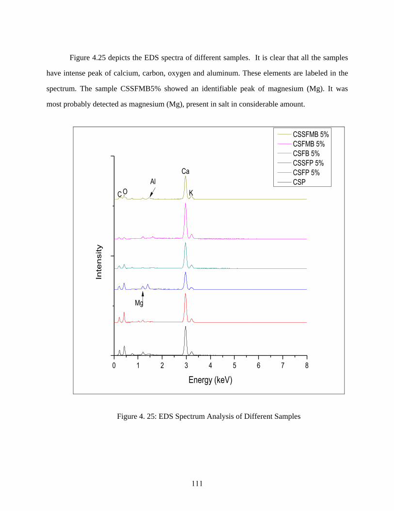
111
Figure 4.25 depicts the EDS spectra of different samples. It is clear that all the samples
have intense peak of calcium, carbon, oxygen and aluminum. These elements are labeled in the
spectrum. The sample CSSFMB5% showed an identifiable peak of magnesium (Mg). It was
most probably detected as magnesium (Mg), present in salt in considerable amount.
0 1 2 3 4 5 6 7 8
Inte
nsity
Energy (keV)
CSSFMB 5%
CSFMB 5%
CSFB 5%
CSSFP 5%
CSFP 5%
CSP
Ca
KOC
Al
Mg
Figure 4. 25: EDS Spectrum Analysis of Different Samples
112
A spot analysis was also performed on CSFB 5% sample. This point was marked in
Figure 4.24 (a) and selected where bacteria was impregnated over calcite crystal. EDS analysis
of this point showed remarkably high percentage of calcium. About 80% by weight calcium
amount on the spot verified the association of bacteria cell with crystal to serve as nucleation site
for biomineralization process (Stocks Fischer et al., 1999).
113
Chapter 5: Summary and Conclusions
The main purpose of this thesis is to describe the use of total dissolved solid (TDS), a
byproduct produced during desalination in a sustainable environmentally friendly way, as a
means of partial replacement of sand in mortar. However, addition of TDS which contains highly
concentrated sodium chloride (NaCl) may weaken the integrity of the cement matrix, resulting in
lower strength of mortar. To minimize loss in strength and reduce leaching of salt, fly ash and
aerobic bacteria were used. The use of fly ash increases the strength and durability while
reducing required cement content. Any reduction in cement content translates into reduction in
carbon footprint because fly ash is a byproduct. In addition, fly ash creates optimum environment
for bacterial growth by lowering pH of mortar matrix.
The aerobic bacteria were also used to increase compressive strength and stabilize salt by
calcite precipitation and by minimizing porosity. Since addition of salt increases pH of the
mortar environment, the survivability of bacteria becomes an issue. To survive in a high pH
(around 12) mortar environment, the bacteria were mutated by exposing them to ultraviolet rays.
The advantage of mutation is that the bacteria can withstand higher pH as well as forms more
calcite than normal bacteria. The use of mutated bacteria in association with fly ash not only
creates finer pores (for better aeration) for bacterial growth, but also it lowers the pH of the
mortar matrix by consuming free lime or calcium hydroxide, formed during hydration of cement.
The mutated bacteria, fly ash and salt/TDS were used to prepare mortar specimens. These
various types of specimens were subjected to strength and durability tests, including freeze thaw
test, water permeability test and absorption test.
The following conclusions can be drawn based on the analysis of all the test results generated
in the course of this investigation:
1. Use of sodium phosphate buffer (Na3PO4) did not affect the 28 day compressive strength
compared to samples prepared with water. The main reason for using sodium phosphate

114
buffer instead of water is that bacteria cells may lyse due to osmotic pressure when added
to water.
2. 5 % replacement of salt reduced the 28 day compressive strength of sample by 5 percent
from control sample, but replacement of 5 percent fly ash by cement amended the
strength of specimens more than 25 percent due to pozzolanic activity.
3. Mutated Bacillus pasteurii and normal B. pasteurii added samples had highest 28 day
compressive strength. Also mutated bacteria and fly ash treated salt samples had showed
improvement in strength from fly ash and salt added samples. This strength development
is due to precipitation of calcite over the surface and pores by microbial activity.
4. Mutated bacteria and fly ash treated samples exhibited better resistance against freezing
and thawing. The sample prepared with mutated bacteria, fly ash and salt have about 43
percent less mortar disintegration than control specimen.
5. The sample with salt and fly ash had the highest permeability and porosity. But, bacteria
treated samples are more impermeable than other samples. Furthermore, specimens
prepared with fly ash were less porous in comparison to the control specimen.
6. From the absorption test it had been found that salt and fly ash-added samples had the
highest absorption rate. However, bacteria and fly ash-treated samples had the lowest
absorption rate due to plugging of pores by calcite. Mutated bacteria and fly ash
improved salt-added samples absorption rate similar to the control specimen. However,
this type of sample (CSSFMB 5%) leached more sodium, chlorine and calcium ions than
samples prepared with fly ash and salt (CSSFP 5%). This result might be biased, as
chemicals used in various steps of mixing and curing of bacteria treated samples may
influence the amount of ion leached in deionized water. For this reason, a more
sophisticated testing needs to be performed to determine the leaching element effect on
the environment.
7. X-ray diffraction analysis of bacteria-treated samples displayed a larger calcite peak as
well as a new phase of silicate (Gehlenite) matrix, which formed due to calcium

115
precipitation, that reacts with the glassy phase to produce dicalcium aluminium
aluminosilicate [Ca2Al(AlSiO7)].
8. SEM investigation indicated full growth of calcite crystal in bacteria-treated samples and
presence of more calcium in those samples. An energy dispersive X-ray spectroscopy
analysis on bacteria embedded sites revealed 80 percent calcium, which verifies that
bacteria cells served as nucleation sites to deposit calcite.
5.1 Suggestions for Future Research
The findings presented in this thesis provided better understanding how aerobic microbial
activity precipitated calcium carbonate over the surface and insides pores to amend mortar
properties, influence of fly ash particle size and its mineralogy on compressive strength, TDS
impact on compressive strength and durability. To better understand microbial activity and TDS
influence, the following issues need further investigation.
The TDS, fly ash and bacteria were used to prepare samples with only one
bacteria cell concentration (OD600=0.6), but as addition of TDS increases the overall pH
of the PCC environment, that may lyse bacteria cells or turn them into endospores.
Therefore, a further investigation should be done by varying the bacteria concentration to
determine the impact on strength and durability of the mortar or PCC.
It is necessary to identify the effect of bacterial activity in presence of
other supplementary cementitious materials like silica fume, slag on concrete or mortar
specimens.
Use of anaerobic bacteria (like Shewanella species) should be investigated
to identify its influence on strength and durability of concrete and mortar by calcite
precipitation. The advantage of using anaerobic bacteria over aerobic bacteria is it does
not require oxygen for metabolic activity and can actively deposit calcite, even after
pores are plugged, as long as nourishment is available.
116
This research did not focus on how permeability was influenced owing to
calcite deposition by biotic activity. Due to complex relationship of permeability with
porosity, pore size and pore connectivity. A more sophisticated approach can be adopted
to develop that relationship.
Calcium carbonate can dissolve in an acidic environment. So, an
experiment can be conducted to inspect the effect of acidic rain on durability of
biologically deposited layer. It is known that biologically produced calcite possesses
more resistance to dissolution that inorganically precipitated calcite.
Titanium dioxide, carbon nanotubes etc. nanoparticles can be used in
conjunction with bacteria to investigate the impact on concrete or mortar for future green
construction.

117
References
ACI Committee 232 Use of Fly Ash in Concrete. - Detroit : ACI 232.2R-96, 1996.
Abdun-Nur Edward. “Fly ash in Concrete, An Evaluation”. Washington, C : Highway
Research Board, 1961. p. 138.
Achal, V.; Mukherjee, A.; Basu, P. C.; Reddy, M. Sudhakara. “Strain improvement of
Sporosarcina pasteurii for enhanced urease and calcite production.” India Microbiol Biotechnol.,
2009, p. 981-988.
Achal, V.; Mukherjee, A.; Reddy, M.S. “Microbial Concrete: A way to enhance the
durability of Building Structures.” Journals of Materials in Civil Engineering, 2010.
ASM Handbook, Volume 10; Materials Characterization. ASM international, The
materials information society, 1986.
ASTM Power Diffraction file, Joint Committee on Powder Diffraction Standards
(JCPDS), Philadelphia, PA, 1941.
Auerbach C. Mutation Research. London : Chapman & Hall, 1976.
Bazylinski .A. and Frankel R.B. “Biologically Induced Mineralization by Bacteria.”
Reviews in Mineralogy and Geochemistry, 54, 2003, p. 95-114.
Belkova LN. “Biomineralization in natural environments: the effect of microorganisms
inhabiting hot spring water and biomats on mineral formation.” Geophys Res Abs, 200 , p. 7.
Berke N.S., Pfeifer .W. and Weil T.G. “Protection against Chloride Induced
Corrosion.” Concrete International, V.10, No.12, 1988, p. 45-55.
Berry E. E. and Malhotra V. M. “Fly Ash for Use in Concrete.” ACI Journal,Proceedings
V. 77, No. 2.,1980, p. 59-73.
Bhardwaj, M. C.; Batra, V. S.; and Sastry, V. V. “Effect of Admixtures (Calcium
Chloride) on Pozzalana Concrete.” Indian Concrete Journal (Bombay), V. 54, No. 5. – 1980, p.
134-138.
118
Bird J. M. and Putman G. W. “Natural analog system for reducing permeability of
ground.” Patent 7, 381, 014. USA, Washington, 2008.
Blick, Ronald L., Peterso C.F., Winter, M. E. “Proportioning and Controlling High
Strength Concrete.” 1 1-163 : American Concret Institute, 1974, p. 141-163.
Bouquet, E.; Boronat, A.; Ramos-Cormenzana, A. “Production of calcite (calcium
carbonate) crystals by soil bacteria in a general phenomenon”. Nature, 246, 1973, p. 527-529.
Bright H. “Biosensors for the future.” Nav Res Rev., 1994, p 46-49.
Brink R. H. and Halstead W. J. “Studies Relating to the Testing of Fly Ash for Use in
Concrete.” ASTM, V. 56. Philadelphia, ASTM, V. 56, 1956, p. 1161-1206.
Burne R. A. and Chen Y. M. “Bacterial ureases in infectious diseases.” Microbes and
Infection, 2, 2000, p. 533-542.
Castanier S., Le Métayer Levrel G. and Perthuisot J. “Ca-carbonates precipitation and
limestone genesis.” The microbiogeologist point of view, Sedimentary Geology, 126, 1999, p 9-
23.
Committee on Advancing Desalination Technology Desalination: A National
Perspective. Washington D.C. National Research Council, 2008.
Demirel, T.; Pitt, J.M.; Schlorholtz, S.M.; Allenstein, R.J.; Hammerberg, R.J.
“Characterization of Fly Ash for Use in Concrete.” IOWA, ISUERI-AMES-84431, 1983.
Desalination: A National Perspective. Washington D.C. National Research Council,
2008.
DESWARE: Encyclopedia of Desalination and Water Resources.
http://www.desware.net/desa4.aspx, 2012.
Diamond Sidney, Flores Lopez and Fedrico "On the Distinction in Physical and Chemical
Characteristics Between Lignitic Bituminous fly ashes" and "Comparative Studies of the Effects
of Lignitic and Bituminous Fly Ashes in Hydrated Cement System" Proceedings, Symposium on
Effects of Fly Ash Incorporate in Cement and Concrete. - Pittsburg , 1981. p. 34-44 and 112-123.

119
iamond, Sydney; Skalny, J.; and Roy, .M. “Effects of Blending Materials on the
Rheology of cement Pastes and Concretes.” Proceedings, Symposium M, Concrete Rhology,
Materials Research Society, Pittsburg, 1982, p.152-173.
Dick, J.; De Windt, W.; De Graef, B.; Saveyn, H.; Van der Meeren, P.; De Belie, N.;
Verstraete, W. “Bio-deposition of a calcium carbonate layer on degraded limestone by Bacillus
species.” Biodegradation 17, 2006, p. 3 7–367.
Dionex ICS-2100 Ion Chromatography System Operator Dionex ICS-2100 Ion
Chromatography System Operator's Manual.
Dmitri Kopeliovich (2009). http://www.substech.com/ dokuwiki/ doku.php?
id=scanning_electron_microscope “Scanning electron microscope.” (May 15, 2011.)
ouglas S. and Beveridge T. J. “Mineral formation by bacteria in natural microbial
communities.” FEMS Microbiol, Ecol. 26, 1998, p 79-88.
Einav R., Harussi K. and Perry . “The footprint of the desalination processes on the
environment.” esalination, 1 2, 2002.
Faibish R.S., Elimelech M. and Cohen Y. “Effect of interparticle electrostatic double
layer interactions on permeable flux decline in crossflow membrane filtration of colloidal
suspensions: an experimental investigation.” J. Colloid Interf. Sci. 20 , 1998, p.77–86.
Fisher, G.L; Prentice, B.A; Silberman, D.; Ondov, J.M.; Ragaini, R.C; Bierman, A.H;
McFarland, A.R.; Pawley, J.B. “Size-dependance of the physical and chemical properties of coal
fly ash.” American Chemical Society meeting, Montreal, Canada, May 1977,p. 149-155.
Frankel R. B. and Bazylinski . A. “Biologically Induced Mineralization by Bacteria.”
Reviews in Mineralogy and Geochemistry, 54, 2003, p 95-114.
Friedrich Widdel Theory and Measurement of Bacterial Growth. 2010.
George .O., Okwadha and Jin Li. ‘Optimum conditions for microbial carbonate
precipitation.” Chemosphere 81, 2010, p. 11 3-1148.

120
Ghosh, P; Mandal, S; Pal, S; Bandyopadhyaya, G; Chattopadhyay, B . “ evelopment of
bioconcrete material using an enrichment culture of novel thermophilic anaerobic bacteria.”
Indian J Exp Biol, 44(4): 2006, p. 336-339.
Ghosh, P.; Mandal, S.; Chattopadhyay, B. .; Pal, S. “Use of microorganism to improve
the strength of cement mortar.” Cem. Concr. Res. 35, 2005, p. 1980-1983.
Ghosh, S.; Biswas, M.; Chattopadhyay, B. .; Mandal, S. “Microbial activity on the
microstructure of bacteria modified mortar.” Cement & Concrete Composites 31, 2009, p.93–98.
Gregory J., McCarthy; Kevin D., Swanson; Lindsay P., Keller; Walter C., Blatte.
“Mineralogy of Western Fly Ash.” Cement and Concrete research V.1 , No. , July. – 1984, p.
471-478.
Hastead, W.J. “Use of Fly Ash in Concrete.” Transportation Research Board, Research
Program No. 127, 1986, p.32.
Hisham Ettouney and Hisham El- essouki. “Teaching esalination.” esalination 1 1,
2001, p. 109-127.
Hoffman . “Salinity Management.” Management of Farm Irrigation Systems. New
York, American Society of Agricultural Engineers, 1990, p. 667–715.
Idorn G.M. “30 Years with Alkalis in Concrete.” 6th International Conference on Alkalis
in Concrete. Copenhagen. Danish Concrete Society, 1983, p. 21-38.
Idorn, G.M. “Concrete Energy and urability.” Concrete International esign and
Construction, V.6, No.2, 1984, p.13-20.
Introduction to X-ray diffraction http://www.mrl.ucsb.edu/mrl/centralfacilities/xray/xray-
basics/index.html. Materials Research Laboratory. - June 15, 2011.
Jones, B.; Renaut, R.W.; and Rosen, M.R.. “Biogenecity of silica precipitation
aroundgeysers and hot springs vents.” 1997, p. 88–104.
Kaltwasser H., Kramer J. and Conger W.R. “Control of urease formation in certain
aerobic bacteria.” Arch. Microbiol. 81. 1972, p. 178-196.

121
Karim,M. R.; Zain,M. F. M.; Jamil, M.; Lai, F. C.; and Islam, M. N. “Strength
development of mortar and concrete containing fly ash: A review.” International Journal of the
Physical Sciences Vol. 6(17), 2011, p. 4137-4153.
Karol RH. “Chemical grouting and soil stabilization. New York, 3rd Edition, M. ekker,
2003.
King Bruce. “Making Better Concrete: Guidelines to using fly ash for higher quality”.
Knorre H. and Krumbein W. “Bacterial calcification.” Springer-Verlag, Berlin, Germany,
2000.
Konhauser, KO; Ferris,F.G. “ iversity of iron and silica precipitation by microbial mats
in hydrothermal waters.” Implications for Precambrian iron formation, Geology, 1996, p. 323.
Kunz B.A. and Glickman B.W. “The role of pirimidine dymers as premutagenic lesions:
a study of targeted vs untargeted mutagenesis in the lac1 gene of Escherichia coli.” Genetics. 106
1984, p. 347-364.
Lackner, K. S.; Wendt, C. H.; Butt, . P.; Joyce, E. L. Jr.; Sharp, .H. “Carbon dioxide
disposal in carbonate minerals.” Energy, 20(11), 199 , p.11 3-1170.
Lane R.O. and Best J.F. “Properties and Use of Fly Ash in Portland Cement Concrete.”
Concrete International: Design and Conmstruction, V.4, No.7, July. 1982, p. 81-92.
Luke, Wilbur I., 1961, “Nature and istribution of Particles of Various sizes in Fly ash.”
Technical Report No.6-583, U.S. Army Engineer Waterways Experiment Station, Vicksburg,
1961.
Maas, E.V. and Tanji K.K. “Crop Salt Tolerance.” Agricultural Salinity Assessment and
Management. American Society of Civil Engineers, 1990, p. 262-303.
Manmohan . and Mehta P. K. “Influence of Pozzolanic, Slag, and Chemical
Admixtures on Pore Size istribution and Permeability of Hardened Cement Pastes.” Cement,
Concrete, and Aggregates, V. 3, No. 1. 1981, p. 63-67.
Mark W. Rosegrant, Ximing Cai and Sarah A. “Cline Global Water Outlook to 202 .”
International Water Management Institute, 2002.
122
Martell, A.E.; Smith, R.M. “Critical Stability Constants.” Vol. : Inorganic Complexes.
Plenum Press, New York, 1976.
Mather Bryant. “Compressive Strength evelopment of 193 Concrete Mixtures uring
10 Years of Moist Curing.” Vicksburg : U.S. Army Engineer Waterways Experiment, 1965.
Majko, Richard M., and Pistelli, Michel F., “Optimizing the Amount of Class-C Fly Ash
in Concrete Mixtures.” Cement, Concrete and Aggregates, V. 6, No.2, 1984, p. 105-119.
McCarthy G.J, Swanson, K.D., Keller, L.P. and Blatter, W.C. “Mineralogy of western
Fly ash.” Cement and Concrete Research, V.1 , No. , July 198 , p. 71-478.
McCarthy G.J, Johansen, D.M., Steeinwand,S.J. and Thedchanamoorthy, A. “X-Ray
efraction Analysis of Fly Ash.” Advances in X-Ray analysis, V.31, 1988.
Merz MUE. “The biology of carbonate precipitation by cyanobacteria.” 1992, p. 81-102.
Mickley M. C. “Membrane Concentrate isposal: Practices and Regulation (Second
Edition).” enver : U.S. Bureau of Reclamation, 2006.
Miguel A.G. and Tyrrell R.M. “Induction of oxygen-dependent lethal damage by
monochromatic UVB (313) radiation: strand breakage, repair and cell death.” Carciogenesis, . .
1983, p.375-380.
Mitchell A.C. and Ferris F.G. “The co-precipitation of Sr into calcite precipitates induced
by bacterial ureolysis in artificial groundwater: temperature and kinetics dependence.” Geochim.
Cosmochim. Acta 69. 2005, p.4199–4210.
Mukherjee, P.K.; Loughborough, M.T.; and Malhotra, V.M. “ evelopment of High-
Strength Concrete Incorporating a Large Percentage of Fly Ash and Superplasticizers.” Cement,
Concrete, and Aggregates.
Muynck, W. .; Belie, N. .; Cox, K. “Bacterial carbonate precipitation reduces the
permeability of cementitious materials.” Sustainable Construction Materials and Technologies,
London, 2007..
Mohamed A.M.O. and Antia H.E. Geoenvironmental Engineering, Elsevier Science. –
1998, p. 707.V.4, No.2,1982, p.72-78.
123
Nemati M. and Voordouw G. “Modification of porous media permeability using calcium
carbonate produced enzymatically in situ.” Enzyme Microb. Technol. 33. 2003, p. 635–642.
Newnham RE. “Molecular mechanisms in smart materials.” Mater Res Soc Bull. 1997, p
20–33.
Neithalath, N.; Weiss, J.; Olek, J. “Predicting the permeability of pervious concrete
(Enhanced Porosity Concrete) from non-destructive electrical measurements.”
Park, Sung-Jin; Yu-Mi, Park; Young Chun, Woo; Jung Kim, Wha; Youl Ghim, Sa.
“Calcite-Forming Bacteria for Compressive Strength Improvement in Mortar.” J. Microbiol.
Biotechnol. (2010), 20(4). 2009, p.782–788.
PCA, Portland Cement Association CD-ROM.
P. Glueckstern, “ esalination-1996 status and trends.” Mekorot, Tel Aviv, January 1997.
Powers, T.C., Copeland, L.E., and Mann, H.M. “Capillary Continuity or iscontinuity in
Cement Pastes.” Journal of PCA Research and evelopment Labs, V. 1, No. 2 ,1959, p. 1-12.
Raask Erich Mineral. “Impurities in Coal Combustion: Behavior, Problems, and
Remedial Measures.” Hemisphere Publishing Corporation, 198 .
Ramachandran SK, Ramakrishnan V and Bang SS. “Remediation of concrete using
microorganism.” ACI Material Journal; 98(1). 2001, p.3-9.
Rhoades J. . and Loveday J. Salinity in irrigated agriculture. “Irrigation of Agricultural
Crops”, American Society of Agronomy. Wisconsin, 1990, p. 1089–1142.
Roh, Y.; Phelps, T. J.; McMillan, A. D.; Lauf, R. J. “Utilization of biomineralization
processes with fly ash for carbon sequestration.” Washington .C: OE-AC05-00OR22725,
U.S. Department of Energy, 2001.
Roy, ella M.; Lukea, Karen; iamonda, Sidney. “Characterization of Fly Ash and Its
Reactions in Concrete.” Pittsburg : Materials Research Society, 198 .
Silver S., Toth K. and Scribner H. “Facilitated transport of calcium by cells and
subcellular membranes of Bacillus subtilis and Escherichia coli.” J. Bacteriol. 122. 197 , p. 880-
885.

124
Skinner WCH and Jahren HA. “Biomineralization.” Treatise on Geochemistry,vol. 8.
Elsevier; 2003, p. 117–84.
Smith, R. L.; Mearing,M.A.; Raba,C.F. “Utilization of Class C Fly Ash in concrete.” 6th
International Fly Ash Utilization Symposium. Reno, 1982, p. 31.
Stocks Fischer S., Galinat J.K. and Bang S.S. “Microbiological precipitation of CaCO3.”
Soil Biol. Biochem. 31. 1999, p. 1563–1571.
Tarquin Anthony. “High Tech Methods to Reduce Concentrate Volume Prior to
isposal.” El Paso : EL Paso Water Utilities Public Service Board, 2010.
Thomson A. “Murray Reverse-Osmosis Desalination of Seawater Powered by
Photovoltaics Without Batteries.” Loughborough, 2003.
Travis J. “Microchips covered with NA emerge as powerful research tools.” Sci News.
1997, p 144-146.
Tsiourtis X. Nicos Desalination and the Environment. Desalination 141. 2001. p. 232-
236.
Varenyam Achal, Xiangliang Pana and Nilüfer Özyurtb “Improved strength and
durability of fly ash-amended concrete by microbial calcite precipitation.” Ecological
Engineering 37. 2011, p. 554–559.
Verbeck, George. “Chemistry of the Hydration of Portland Cement.” Proceedings, th
International Symposium on the Chemistry of Cement (Washington, D.C., Oct), Monograph No.
43, U.S. National Bureau of Standards, Washington, D.C., p.453-465.
Vivek Tandon and Miguel Picornell. “Recycled materials in vertical moisture barriers.” -
El Paso: Center for Geotechnical and Highway Materials, 1996.
Whiting, .; and W. ziedzic. “Behavior of cement-reduced and flowing fresh concretes
containing conventional water-reducing and second generation high-range water-reducing
admixtures.” Cement, concrete, and Aggregates 11 (1), 1989, p.30-39.
Will Perkins. “Fly Ash in Concrete.” November 2011.

125
Witkin E.M. “ Ultraviolet mutagenesis and inducible NA repair in Escherichia coli.”
Bacteriol. Rev. 40. 1976, p. 869-907.

126
Appendix A
Water Permeability Test Data

127
Table A-1: CSP Sample 1 test data
DATE CAST: 3/29/2012
Cross sectional
area of Graduated
cylinder
8.042477193 cm2
SAMPLE SIZE: 4X4 in cylinder
DATE TEST: 4/6/2012
Average Effluent
volume flow
rate,Q (mL/s)=
∆V/∆t 2.68
Atmospheric pressure,P ambient= 101325 Pa
Length of Specimen,m= 0.1016
Cross-Sectional
area of specimen
perpendicular to
direction of flow,
A(m2)=
0.00810731
Viscosity of Water, µw(Pa.s)= 9.3250E-04
Sp. Gravity of Water (Pa/cm) : 9.8
Intrinsic
Permeability,k 8.56398E-12 m2
Q µwL/(A∆P)
Sat. Surface Dry Wt. of
Specimen (g): 1651.1
Coefficient of
Permeability
(m/s)
9.00E-06
Dry Wt. of Specimen (g): 1449
Volume of Water
(ml)=Volume of Void (cm3) 202.1
Porosity (ɳ)= 25 %
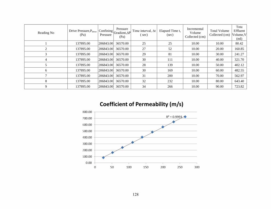
128
Reading No Drive Pressure,Pdrive
(Pa)
Confining
Pressure
Pressure
Gradient,∆P
(Pa)
Time interval, ∆t
( sec)
Elapsed Time t,
(sec)
Incremental
Volume
Collected (cm)
Total Volume
Collected (cm)
Tota
Effluent
Volume,V
(ml)
1 137895.00 206843.00 36570.00 25 25 10.00 10.00 80.42
2 137895.00 206843.00 36570.00 27 52 10.00 20.00 160.85
3 137895.00 206843.00 36570.00 29 81 10.00 30.00 241.27
4 137895.00 206843.00 36570.00 30 111 10.00 40.00 321.70
5 137895.00 206843.00 36570.00 28 139 10.00 50.00 402.12
6 137895.00 206843.00 36570.00 30 169 10.00 60.00 482.55
7 137895.00 206843.00 36570.00 31 200 10.00 70.00 562.97
8 137895.00 206843.00 36570.00 32 232 10.00 80.00 643.40
9 137895.00 206843.00 36570.00 34 266 10.00 90.00 723.82

129
Table A-2: CSP Sample 2 test data
DATE CAST: 3/29/2012
Cross sectional
area of Graduated
cylinder
8.042477193 cm2
SAMPLE SIZE: 4X4 in cylinder
DATE TEST: 4/6/2012
Average Effluent
volume flow
rate,Q (mL/s)=
∆V/∆t 3.17
Atmospheric pressure,P ambient= 101325 Pa
Length of Specimen,m= 0.1016
Cross-Sectional
area of specimen
perpendicular to
direction of flow,
A(m2)=
0.00810731
Viscosity of Water, µw(Pa.s)= 9.3250E-04
Sp. Gravity of Water (Pa/cm) : 9.8
Intrinsic
Permeability,k 1.01298E-11 m2
Q µwL/(A∆P)
Sat. Surface Dry Wt. of
Specimen (g): 1625.1
Coefficient of
Permeability
(m/s)
1.06E-05
Dry Wt. of Specimen (g): 1415
Volume of Water
(ml)=Volume of Void (cm3) 210.1
Porosity (ɳ)= 26 %

130
Reading No Drive Pressure,Pdrive
(Pa)
Confining
Pressure
Pressure
Gradient,∆P
(Pa)
Time interval, ∆t
( sec)
Elapsed Time t,
(sec)
Incremental
Volume
Collected (cm)
Total Volume
Collected (cm)
Tota
Effluent
Volume,V
(ml)
1 137895.00 206843.00 36570.00 21 21 10.00 10.00 80.42
2 137895.00 206843.00 36570.00 22 43 10.00 20.00 160.85
3 137895.00 206843.00 36570.00 23 66 10.00 30.00 241.27
4 137895.00 206843.00 36570.00 23 89 10.00 40.00 321.70
5 137895.00 206843.00 36570.00 24 113 10.00 50.00 402.12
6 137895.00 206843.00 36570.00 25 138 10.00 60.00 482.55
7 137895.00 206843.00 36570.00 25 163 10.00 70.00 562.97
8 137895.00 206843.00 36570.00 26 189 10.00 80.00 643.40
9 137895.00 206843.00 36570.00 27 216 10.00 90.00 723.82
10 137895.00 206843.00 36570.00 26 242 10.00 100.00 804.25
11 137895.00 206843.00 36570.00 27 269 10.00 110.00 884.67
12 137895.00 206843.00 36570.00 27 296 10.00 120.00 965.10
13 137895.00 206843.00 36570.00 28 324 10.00 130.00 1045.52

131
Table A-3: CSFP 5% Sample 1 test data
DATE CAST: 1/28/2012
Cross sectional
area of Graduated
cylinder
8.042477193 cm2
SAMPLE SIZE: 4X4 in cylinder
DATE TEST: 3/16/2012
Average Effluent
volume flow
rate,Q (mL/s)=
∆V/∆t 2.181
Atmospheric pressure,P ambient= 101325 Pa
Length of Specimen,m= 0.1016
Cross-Sectional
area of specimen
perpendicular to
direction of flow,
A(m2)=
0.00810731
Viscosity of Water, µw(Pa.s)= 9.3250E-04
Sp. Gravity of Water (Pa/cm) : 9.8
Intrinsic
Permeability,k 6.97E-12 m2
Q µwL/(A∆P)
Sat. Surface Dry Wt. of
Specimen (g): 1677.3
Coefficient of
Permeability
(m/s)
7.32E-06
Dry Wt. of Specimen (g): 1493.7
Volume of Water
(ml)=Volume of Void (cm3) 183.6
Porosity (ɳ)= 22 %
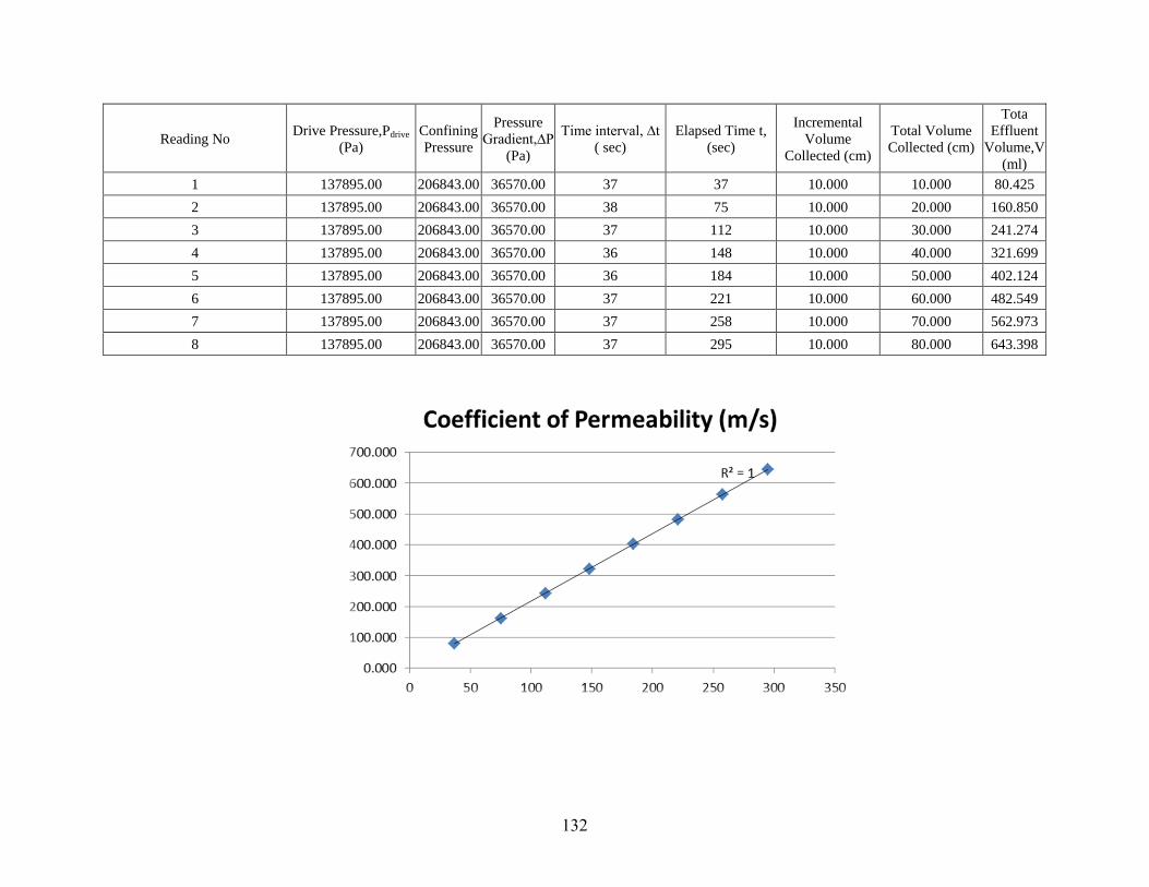
132
Reading No Drive Pressure,Pdrive
(Pa)
Confining
Pressure
Pressure
Gradient,∆P
(Pa)
Time interval, ∆t
( sec)
Elapsed Time t,
(sec)
Incremental
Volume
Collected (cm)
Total Volume
Collected (cm)
Tota
Effluent
Volume,V
(ml)
1 137895.00 206843.00 36570.00 37 37 10.000 10.000 80.425
2 137895.00 206843.00 36570.00 38 75 10.000 20.000 160.850
3 137895.00 206843.00 36570.00 37 112 10.000 30.000 241.274
4 137895.00 206843.00 36570.00 36 148 10.000 40.000 321.699
5 137895.00 206843.00 36570.00 36 184 10.000 50.000 402.124
6 137895.00 206843.00 36570.00 37 221 10.000 60.000 482.549
7 137895.00 206843.00 36570.00 37 258 10.000 70.000 562.973
8 137895.00 206843.00 36570.00 37 295 10.000 80.000 643.398

133
Table A-4: CSFP 5% Sample 2 test data
DATE CAST: 1/28/2012
Cross sectional
area of Graduated
cylinder
8.042477193 cm2
SAMPLE SIZE: 4X4 in cylinder
DATE TEST: 3/16/2012
Average Effluent
volume flow
rate,Q (mL/s)=
∆V/∆t 1.9048
Atmospheric pressure,P ambient= 101325 Pa
Length of Specimen,m= 0.1016
Cross-Sectional
area of specimen
perpendicular to
direction of flow,
A(m2)=
0.00810731
Viscosity of Water, µw(Pa.s)= 9.3250E-04
Sp. Gravity of Water (Pa/cm) : 9.8
Intrinsic
Permeability,k 6.09E-12 m2
Q µwL/(A∆P)
Sat. Surface Dry Wt. of Specimen
(g): 1670
Coefficient of
Permeability
(m/s)
6.40E-06
Dry Wt. of Specimen (g): 1490.6
Volume of Water (ml)=Volume of
Void (cm3) 179.4
Porosity (ɳ)= 22 %

134
Reading No Drive Pressure,Pdrive
(Pa)
Confining
Pressure
Pressure
Gradient,∆P
(Pa)
Time interval, ∆t
( sec)
Elapsed Time t,
(sec)
Incremental
Volume
Collected (cm)
Total Volume
Collected (cm)
Tota
Effluent
Volume,V
(ml)
1 137895.00 206843.00 36570.00 40 40 10.000 10.000 80.425
2 137895.00 206843.00 36570.00 41 81 10.000 20.000 160.850
3 137895.00 206843.00 36570.00 42 123 10.000 30.000 241.274
4 137895.00 206843.00 36570.00 41 164 10.000 40.000 321.699
5 137895.00 206843.00 36570.00 42 206 10.000 50.000 402.124
6 137895.00 206843.00 36570.00 43 249 10.000 60.000 482.549
7 137895.00 206843.00 36570.00 43 292 10.000 70.000 562.973
8 137895.00 206843.00 36570.00 44 336 10.000 80.000 643.398
9 137895.00 206843.00 36570.00 44 380 10.000 90.000 723.823
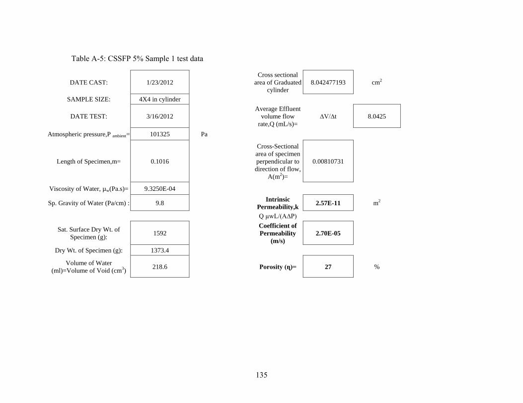
135
Table A-5: CSSFP 5% Sample 1 test data
DATE CAST: 1/23/2012
Cross sectional
area of Graduated
cylinder
8.042477193 cm2
SAMPLE SIZE: 4X4 in cylinder
DATE TEST: 3/16/2012
Average Effluent
volume flow
rate,Q (mL/s)=
∆V/∆t 8.0425
Atmospheric pressure,P ambient= 101325 Pa
Length of Specimen,m= 0.1016
Cross-Sectional
area of specimen
perpendicular to
direction of flow,
A(m2)=
0.00810731
Viscosity of Water, µw(Pa.s)= 9.3250E-04
Sp. Gravity of Water (Pa/cm) : 9.8
Intrinsic
Permeability,k 2.57E-11 m2
Q µwL/(A∆P)
Sat. Surface Dry Wt. of
Specimen (g): 1592
Coefficient of
Permeability
(m/s)
2.70E-05
Dry Wt. of Specimen (g): 1373.4
Volume of Water
(ml)=Volume of Void (cm3) 218.6
Porosity (ɳ)= 27 %

136
Reading No Drive Pressure,Pdrive
(Pa)
Confining
Pressure
Pressure
Gradient,∆P
(Pa)
Time interval, ∆t
( sec)
Elapsed Time t,
(sec)
Incremental
Volume
Collected (cm)
Total Volume
Collected (cm)
Tota
Effluent
Volume,V
(ml)
1 137895.00 206843.00 36570.00 15 15 15.000 15.000 120.637
2 137895.00 206843.00 36570.00 15 30 15.000 30.000 241.274
3 137895.00 206843.00 36570.00 15 45 15.000 45.000 361.911
4 137895.00 206843.00 36570.00 15 60 15.000 60.000 482.549
5 137895.00 206843.00 36570.00 15 75 15.000 75.000 603.186
6 137895.00 206843.00 36570.00 15 90 15.000 90.000 723.823
7 137895.00 206843.00 36570.00 15 105 15.000 105.000 844.460
8 137895.00 206843.00 36570.00 15 120 15.000 120.000 965.097
9 137895.00 206843.00 36570.00 15 135 15.000 135.000 1085.734
10 137895.00 206843.00 36570.00 15 150 15.000 150.000 1206.372
11 137895.00 206843.00 36570.00 15 165 15.000 165.000 1327.009

137
Table A-6: CSSFP 5% Sample 2 test data
DATE CAST: 1/23/2012
Cross sectional
area of Graduated
cylinder
8.042477193 cm2
SAMPLE SIZE: 4X4 in cylinder
DATE TEST: 3/16/2012
Average Effluent
volume flow
rate,Q (mL/s)=
∆V/∆t 6.501395
Atmospheric pressure,P ambient= 101325 Pa
Length of Specimen,m= 0.1016
Cross-Sectional
area of specimen
perpendicular to
direction of flow,
A(m2)=
0.00810731
Viscosity of Water, µw(Pa.s)= 9.3250E-04
Sp. Gravity of Water (Pa/cm) : 9.8
Intrinsic
Permeability,k 2.08E-11 m2
Q µwL/(A∆P)
Sat. Surface Dry Wt. of
Specimen (g): 1638
Coefficient of
Permeability
(m/s)
2.18E-05
Dry Wt. of Specimen (g): 1404
Volume of Water
(ml)=Volume of Void (cm3) 234
Porosity (ɳ)= 28 %

138
Reading No Drive Pressure,Pdrive
(Pa)
Confining
Pressure
Pressure
Gradient,∆P
(Pa)
Time interval, ∆t
( sec)
Elapsed Time t,
(sec)
Incremental
Volume
Collected (cm)
Total Volume
Collected (cm)
Tota
Effluent
Volume,V
(ml)
1 137895.00 206843.00 36570.00 19 19 15.000 15.000 120.637
2 137895.00 206843.00 36570.00 18 37 15.000 30.000 241.274
3 137895.00 206843.00 36570.00 18 55 15.000 45.000 361.911
4 137895.00 206843.00 36570.00 19 74 15.000 60.000 482.549
5 137895.00 206843.00 36570.00 19 93 15.000 75.000 603.186
6 137895.00 206843.00 36570.00 18 111 15.000 90.000 723.823
7 137895.00 206843.00 36570.00 18 129 15.000 105.000 844.460
8 137895.00 206843.00 36570.00 19 148 15.000 120.000 965.097
9 137895.00 206843.00 36570.00 19 167 15.000 135.000 1085.734

139
Table A-7: CSFB 5% Sample test data
DATE CAST: 1/18/2012
Cross sectional
area of Graduated
cylinder
8.042477193 cm2
SAMPLE SIZE: 4X4 in cylinder
DATE TEST: 3/16/2012
Average Effluent
volume flow
rate,Q (mL/s)=
∆V/∆t 2.7170608
Atmospheric pressure,P ambient= 101325 Pa
Length of Specimen,m= 0.1016
Cross-Sectional
area of specimen
perpendicular to
direction of flow,
A(m2)=
0.00810731
Viscosity of Water, µw(Pa.s)= 9.3250E-04
Sp. Gravity of Water (Pa/cm) : 9.8
Intrinsic
Permeability,k 8.68E-12 m2
Q µwL/(A∆P)
Sat. Surface Dry Wt. of
Specimen (g): 1612.6
Coefficient of
Permeability
(m/s)
9.12E-06
Dry Wt. of Specimen (g): 1394.8
Volume of Water
(ml)=Volume of Void (cm3) 217.8
Porosity (ɳ)= 26 %

140
Reading No Drive Pressure,Pdrive
(Pa)
Confining
Pressure
Pressure
Gradient,∆P
(Pa)
Time interval, ∆t
( sec)
Elapsed Time t,
(sec)
Incremental
Volume
Collected (cm)
Total Volume
Collected (cm)
Tota
Effluent
Volume,V
(ml)
1 137895.00 206843.00 36570.00 30 30 10.000 10.000 80.425
2 137895.00 206843.00 36570.00 30 60 10.000 20.000 160.850
3 137895.00 206843.00 36570.00 29 89 10.000 30.000 241.274
4 137895.00 206843.00 36570.00 29 118 10.000 40.000 321.699
5 137895.00 206843.00 36570.00 30 148 10.000 50.000 402.124
6 137895.00 206843.00 36570.00 30 178 10.000 60.000 482.549
7 137895.00 206843.00 36570.00 30 208 10.000 70.000 562.973
8 137895.00 206843.00 36570.00 30 238 10.000 80.000 643.398
9 137895.00 206843.00 36570.00 29 267 10.000 90.000 723.823
10 137895.00 206843.00 36570.00 29 296 10.000 100.000 804.248
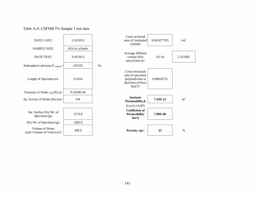
141
Table A-8: CSFMB 5% Sample 1 test data
DATE CAST: 1/14/2012
Cross sectional
area of Graduated
cylinder
8.042477193 cm2
SAMPLE SIZE: 4X4 in cylinder
DATE TEST: 3/16/2012
Average Effluent
volume flow
rate,Q (mL/s)=
∆V/∆t 2.321982
Atmospheric pressure,P ambient= 101325 Pa
Length of Specimen,m= 0.1016
Cross-Sectional
area of specimen
perpendicular to
direction of flow,
A(m2)=
0.00810731
Viscosity of Water, µw(Pa.s)= 9.3250E-04
Sp. Gravity of Water (Pa/cm) : 9.8
Intrinsic
Permeability,k 7.42E-12 m2
Q µwL/(A∆P)
Sat. Surface Dry Wt. of
Specimen (g): 1574.8
Coefficient of
Permeability
(m/s)
7.80E-06
Dry Wt. of Specimen (g): 1365.9
Volume of Water
(ml)=Volume of Void (cm3) 208.9
Porosity (ɳ)= 25 %
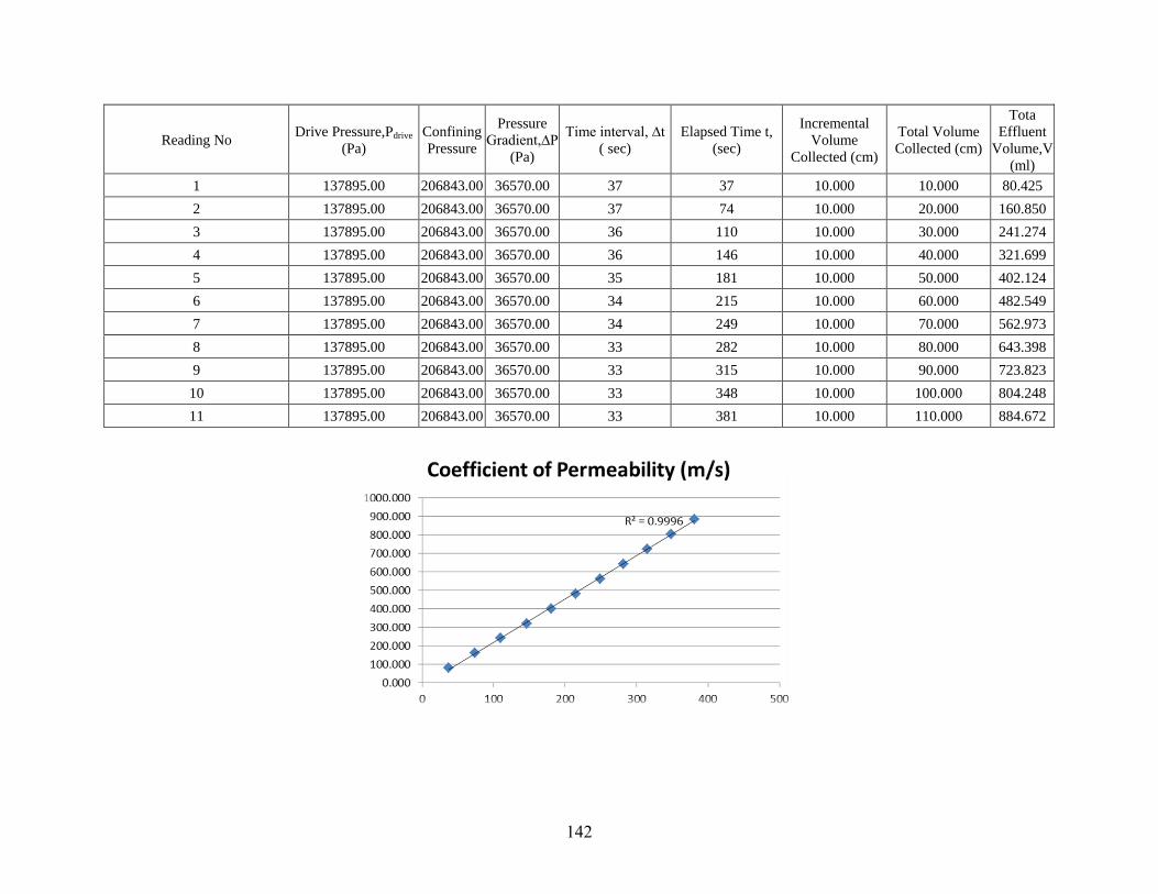
142
Reading No Drive Pressure,Pdrive
(Pa)
Confining
Pressure
Pressure
Gradient,∆P
(Pa)
Time interval, ∆t
( sec)
Elapsed Time t,
(sec)
Incremental
Volume
Collected (cm)
Total Volume
Collected (cm)
Tota
Effluent
Volume,V
(ml)
1 137895.00 206843.00 36570.00 37 37 10.000 10.000 80.425
2 137895.00 206843.00 36570.00 37 74 10.000 20.000 160.850
3 137895.00 206843.00 36570.00 36 110 10.000 30.000 241.274
4 137895.00 206843.00 36570.00 36 146 10.000 40.000 321.699
5 137895.00 206843.00 36570.00 35 181 10.000 50.000 402.124
6 137895.00 206843.00 36570.00 34 215 10.000 60.000 482.549
7 137895.00 206843.00 36570.00 34 249 10.000 70.000 562.973
8 137895.00 206843.00 36570.00 33 282 10.000 80.000 643.398
9 137895.00 206843.00 36570.00 33 315 10.000 90.000 723.823
10 137895.00 206843.00 36570.00 33 348 10.000 100.000 804.248
11 137895.00 206843.00 36570.00 33 381 10.000 110.000 884.672
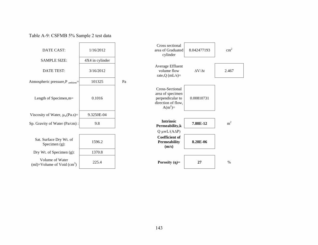
143
Table A-9: CSFMB 5% Sample 2 test data
DATE CAST: 1/16/2012
Cross sectional
area of Graduated
cylinder
8.042477193 cm2
SAMPLE SIZE: 4X4 in cylinder
DATE TEST: 3/16/2012
Average Effluent
volume flow
rate,Q (mL/s)=
∆V/∆t 2.467
Atmospheric pressure,P ambient= 101325 Pa
Length of Specimen,m= 0.1016
Cross-Sectional
area of specimen
perpendicular to
direction of flow,
A(m2)=
0.00810731
Viscosity of Water, µw(Pa.s)= 9.3250E-04
Sp. Gravity of Water (Pa/cm) : 9.8
Intrinsic
Permeability,k 7.88E-12 m2
Q µwL/(A∆P)
Sat. Surface Dry Wt. of
Specimen (g): 1596.2
Coefficient of
Permeability
(m/s)
8.28E-06
Dry Wt. of Specimen (g): 1370.8
Volume of Water
(ml)=Volume of Void (cm3) 225.4
Porosity (ɳ)= 27 %

144
Reading No Drive Pressure,Pdrive
(Pa)
Confining
Pressure
Pressure
Gradient,∆P
(Pa)
Time interval, ∆t
( sec)
Elapsed Time t,
(sec)
Incremental
Volume
Collected (cm)
Total Volume
Collected (cm)
Tota
Effluent
Volume,V
(ml)
1 137895.00 206843.00 36570.00 34 34 10.000 10.000 80.425
2 137895.00 206843.00 36570.00 34 68 10.000 20.000 160.850
3 137895.00 206843.00 36570.00 33 101 10.000 30.000 241.274
4 137895.00 206843.00 36570.00 33 134 10.000 40.000 321.699
5 137895.00 206843.00 36570.00 33 167 10.000 50.000 402.124
6 137895.00 206843.00 36570.00 32 199 10.000 60.000 482.549
7 137895.00 206843.00 36570.00 32 231 10.000 70.000 562.973
8 137895.00 206843.00 36570.00 32 263 10.000 80.000 643.398
9 137895.00 206843.00 36570.00 32 295 10.000 90.000 723.823
10 137895.00 206843.00 36570.00 31 326 10.000 100.000 804.248

145
Table A-10: CSSFMB 5% Sample 1 test data
DATE CAST: 1/16/2012
Cross sectional
area of Graduated
cylinder
8.042477193 cm2
SAMPLE SIZE: 4X4 in cylinder
DATE TEST: 3/16/2012
Average Effluent
volume flow
rate,Q (mL/s)=
∆V/∆t 1.4491
Atmospheric pressure,P ambient= 101325 Pa
Length of Specimen,m= 0.1016
Cross-Sectional
area of specimen
perpendicular to
direction of flow,
A(m2)=
0.00810731
Viscosity of Water, µw(Pa.s)= 9.3250E-04
Sp. Gravity of Water (Pa/cm) : 9.8
Intrinsic
Permeability,k 4.63E-12 m2
Q µwL/(A∆P)
Sat. Surface Dry Wt. of
Specimen (g): 1648.3
Coefficient of
Permeability
(m/s)
4.87E-06
Dry Wt. of Specimen (g): 1461.5
Volume of Water
(ml)=Volume of Void (cm3) 186.8
Porosity (ɳ)= 23 %
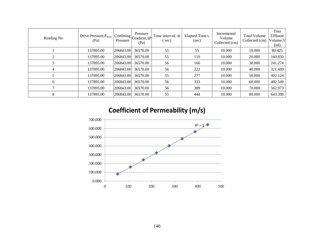
146
Reading No Drive Pressure,Pdrive
(Pa)
Confining
Pressure
Pressure
Gradient,∆P
(Pa)
Time interval, ∆t
( sec)
Elapsed Time t,
(sec)
Incremental
Volume
Collected (cm)
Total Volume
Collected (cm)
Tota
Effluent
Volume,V
(ml)
1 137895.00 206843.00 36570.00 55 55 10.000 10.000 80.425
2 137895.00 206843.00 36570.00 55 110 10.000 20.000 160.850
3 137895.00 206843.00 36570.00 56 166 10.000 30.000 241.274
4 137895.00 206843.00 36570.00 56 222 10.000 40.000 321.699
5 137895.00 206843.00 36570.00 55 277 10.000 50.000 402.124
6 137895.00 206843.00 36570.00 56 333 10.000 60.000 482.549
7 137895.00 206843.00 36570.00 56 389 10.000 70.000 562.973
8 137895.00 206843.00 36570.00 55 444 10.000 80.000 643.398

147
Table A-11: CSSFMB 5% Sample 2 test data
DATE CAST: 1/16/2012
Cross sectional
area of Graduated
cylinder
8.042477193 cm2
SAMPLE SIZE: 4X4 in cylinder
DATE TEST: 3/16/2012
Average Effluent
volume flow
rate,Q (mL/s)=
∆V/∆t 1.008751
Atmospheric pressure,P ambient= 101325 Pa
Length of Specimen,m= 0.1016
Cross-Sectional
area of specimen
perpendicular to
direction of flow,
A(m2)=
0.00810731
Viscosity of Water, µw(Pa.s)= 9.3250E-04
Sp. Gravity of Water (Pa/cm) : 9.8
Intrinsic
Permeability,k 3.22E-12 m2
Q µwL/(A∆P)
Sat. Surface Dry Wt. of
Specimen (g): 1653.6
Coefficient of
Permeability
(m/s)
3.39E-06
Dry Wt. of Specimen (g): 1453.4
Volume of Water
(ml)=Volume of Void (cm3) 200.2
Porosity (ɳ)= 24 %
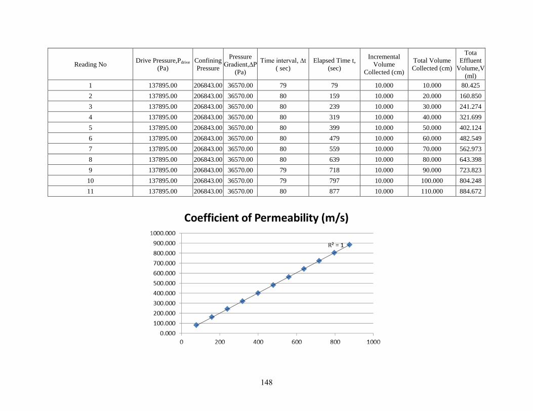
148
Reading No Drive Pressure,Pdrive
(Pa)
Confining
Pressure
Pressure
Gradient,∆P
(Pa)
Time interval, ∆t
( sec)
Elapsed Time t,
(sec)
Incremental
Volume
Collected (cm)
Total Volume
Collected (cm)
Tota
Effluent
Volume,V
(ml)
1 137895.00 206843.00 36570.00 79 79 10.000 10.000 80.425
2 137895.00 206843.00 36570.00 80 159 10.000 20.000 160.850
3 137895.00 206843.00 36570.00 80 239 10.000 30.000 241.274
4 137895.00 206843.00 36570.00 80 319 10.000 40.000 321.699
5 137895.00 206843.00 36570.00 80 399 10.000 50.000 402.124
6 137895.00 206843.00 36570.00 80 479 10.000 60.000 482.549
7 137895.00 206843.00 36570.00 80 559 10.000 70.000 562.973
8 137895.00 206843.00 36570.00 80 639 10.000 80.000 643.398
9 137895.00 206843.00 36570.00 79 718 10.000 90.000 723.823
10 137895.00 206843.00 36570.00 79 797 10.000 100.000 804.248
11 137895.00 206843.00 36570.00 80 877 10.000 110.000 884.672

149
Appendix B
The Absorption Test Data

150
Table B-1: Initial absorption rate of samples
Sample
Sample 1
Initial
Absorption
Rate (x 10-4
mm/s1/2
)
Sample 2
Initial
Absorption
Rate (x 10-4
mm/s1/2
)
Sample 3
Initial
Absorption
Rate (x 10-4
mm/s1/2
)
Mean Standard
deviation CV(%)
Average
Initial
Absorption
Rate (x 10-4
mm/s1/2
)
CSP 163 188 161 170.67 15.04 9 171
CSFP 5% - 136 141 - - - 139
CSFB 5% 138 126 123 129.00 7.94 6 129
CSFMB 5% 131 115 129 125.00 8.72 7 125
CSSFP5% 156 - 226 - - - 191
CSSFMB 5% 173 148 - - - - 160

151
Table B-2: Leaching, pH and Electricla Conductivity (EC) data
Sample
Leaching Element (mg/l) after 8 days Leaching Element (mg/g) of each samples after 8 days Total Ion
mg/g
(dominant
Element)
pH EC(µs/cm)
Cl Na Ca Cl Na Ca initial final ∆ initial final ∆
CSP
6.176 34.899 28.921 0.004 0.024 0.020 0.048 7.150 9.500 2.350 50 360 310
10.484 53.937 24.730 0.007 0.038 0.018 0.063 7.150 9.900 2.750 50 460 410
6.410 62.912 11.381 0.004 0.044 0.008 0.056 7.150 9.700 2.550 50 440 390
CSFP 5%
10.706 59.383 8.207 0.008 0.042 0.006 0.055 7.150 9.610 2.460 50 410 360
4.895 34.560 16.924 0.003 0.024 0.012 0.040 7.150 9.430 2.280 50 310 260
5.569 35.119 18.006 0.004 0.025 0.013 0.041 7.150 9.420 2.270 50 310 260
CSFB 5%
162.091 63.737 68.149 0.113 0.044 0.048 0.205 7.150 7.150 0.000 50 710 660
154.207 58.986 77.054 0.108 0.041 0.054 0.203 7.150 6.930 -0.220 50 670 620
278.631 50.809 143.620 0.195 0.036 0.101 0.331 7.150 6.880 -0.270 50 990 940
CSFMB 5%
281.267 52.604 104.966 0.199 0.037 0.074 0.310 7.150 8.700 1.550 50 1170 1120
246.728 39.727 130.847 0.175 0.028 0.093 0.297 7.150 7.400 0.250 50 1060 1010
436.134 64.278 169.631 0.314 0.046 0.122 0.482 7.150 8.830 1.680 50 1470 1420
CSSFP5%
1056.915 711.734 29.036 0.735 0.495 0.020 1.250 7.150 10.080 2.930 50 3430 3380
1033.200 673.369 34.378 0.715 0.466 0.024 1.205 7.150 10.430 3.280 50 3080 3030
1066.362 671.441 47.772 0.737 0.464 0.033 1.234 7.150 9.880 2.730 50 3410 3360
CSSFMB 5%
1472.285 887.371 41.145 1.091 0.658 0.030 1.780 7.150 9.180 2.030 40 3930 3890
1311.849 774.294 47.180 0.966 0.570 0.035 1.571 7.150 9.000 1.850 40 4230 4190
2275.813 1345.912 53.419 1.713 1.013 0.040 2.766 7.150 9.270 2.120 40 6100 6060
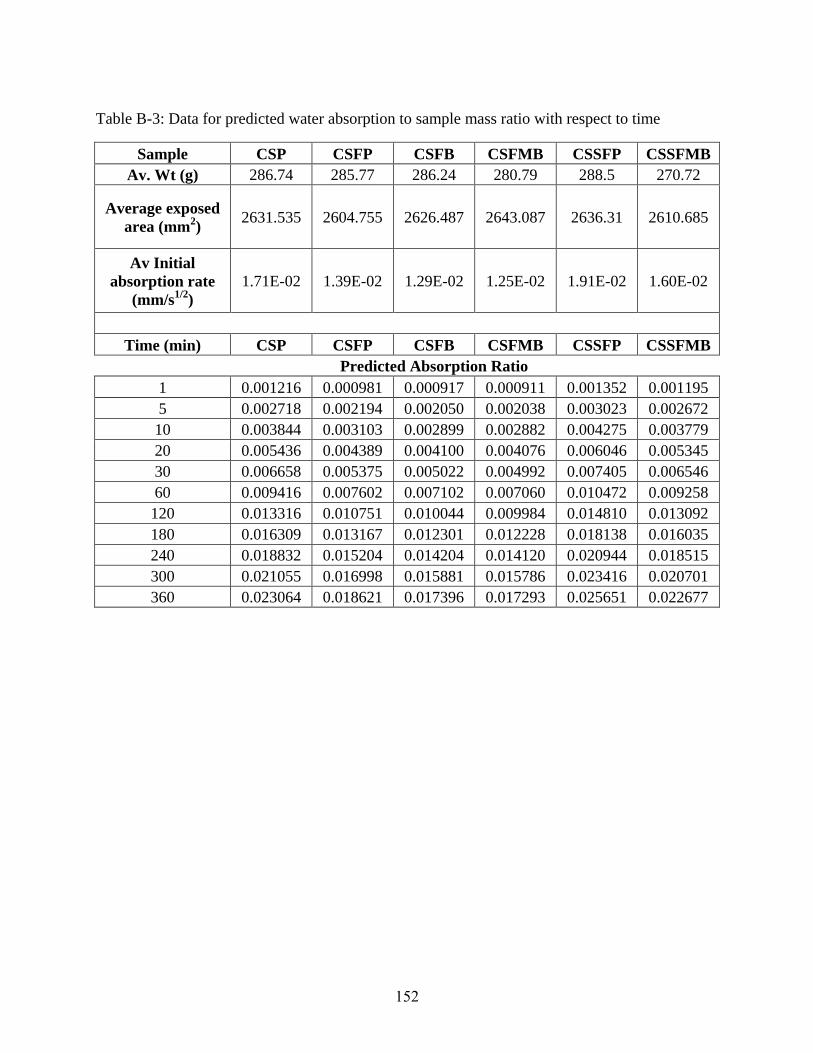
152
Table B-3: Data for predicted water absorption to sample mass ratio with respect to time
Sample CSP CSFP CSFB CSFMB CSSFP CSSFMB
Av. Wt (g) 286.74 285.77 286.24 280.79 288.5 270.72
Average exposed
area (mm2)
2631.535 2604.755 2626.487 2643.087 2636.31 2610.685
Av Initial
absorption rate
(mm/s1/2
)
1.71E-02 1.39E-02 1.29E-02 1.25E-02 1.91E-02 1.60E-02
Time (min) CSP CSFP CSFB CSFMB CSSFP CSSFMB
Predicted Absorption Ratio
1 0.001216 0.000981 0.000917 0.000911 0.001352 0.001195
5 0.002718 0.002194 0.002050 0.002038 0.003023 0.002672
10 0.003844 0.003103 0.002899 0.002882 0.004275 0.003779
20 0.005436 0.004389 0.004100 0.004076 0.006046 0.005345
30 0.006658 0.005375 0.005022 0.004992 0.007405 0.006546
60 0.009416 0.007602 0.007102 0.007060 0.010472 0.009258
120 0.013316 0.010751 0.010044 0.009984 0.014810 0.013092
180 0.016309 0.013167 0.012301 0.012228 0.018138 0.016035
240 0.018832 0.015204 0.014204 0.014120 0.020944 0.018515
300 0.021055 0.016998 0.015881 0.015786 0.023416 0.020701
360 0.023064 0.018621 0.017396 0.017293 0.025651 0.022677
153
Vita
Bijoy Halder was born on December 30, 1984, in Dhaka, Bangladesh. After finishing his
school education, he joined Bangladesh University of Engineering and Technology for his
Bachelor’s Degree and completed his degree in 2007.
From 2007 to 2010, he worked in different construction company of Bangladesh and
Singapore. The experience gained in Singapore actually influenced him to go for higher degree
in Geotechnical engineering and he joined in University of Texas at El Paso for his master’s
degree in August 2010, in the school of Civil Engineering.