SURVIVAL DATA ANALYSIS - MRC Biostatistics Unit · Survival and Hazard Functions • Survival and hazard functions play prominent roles in survival analysis • S (t) is the probability

Part III/MPhil in Statistical Science 1

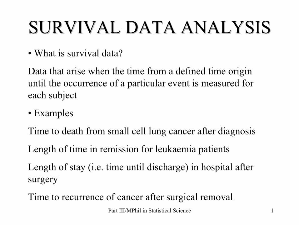
SURVIVAL DATA ANALYSISSURVIVAL DATA ANALYSIS• What is survival data?

Data that arise when the time from a defined time origin until the occurrence of a particular event is measured for each subject

• Examples

Time to death from small cell lung cancer after diagnosis

Length of time in remission for leukaemia patients

Length of stay (i.e. time until discharge) in hospital after surgery

Time to recurrence of cancer after surgical removal


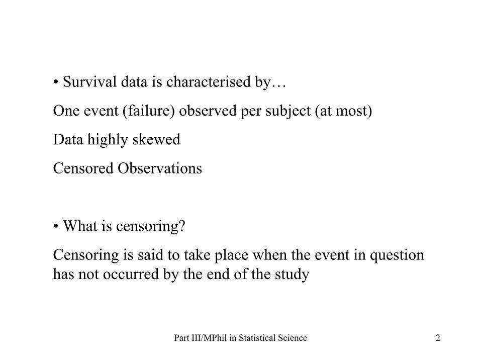
• Survival data is characterised by…

One event (failure) observed per subject (at most)

Data highly skewed

Censored Observations

• What is censoring?

Censoring is said to take place when the event in question has not occurred by the end of the study


• Examples of censoring

Patient still alive

Lost to follow-up (e.g. subject migrated)

Died from an unrelated cause (e.g. car accident)

•

The censoring patterns are of the same form for each situation described above (i.e. right-censoring)

Subjects were observed event-free for certain lengths of time, after which no more information about these subjects is known

True survival times exceed observed survival times


• It is important to find out the reason for censoring

•

We usually assume that the censoring is uninformative, but this need not be the case

• Example

If we are investigating time to death from cancer and a patient dies from a drug overdose. Do we consider this patient as a censored case or uncensored case if we knew that the reason for overdosing on the pain killers was that the cancer had extensively metastasised and the resulting pain was too much for the person to cope with?

•

However, in the absence of further information we treat as censored


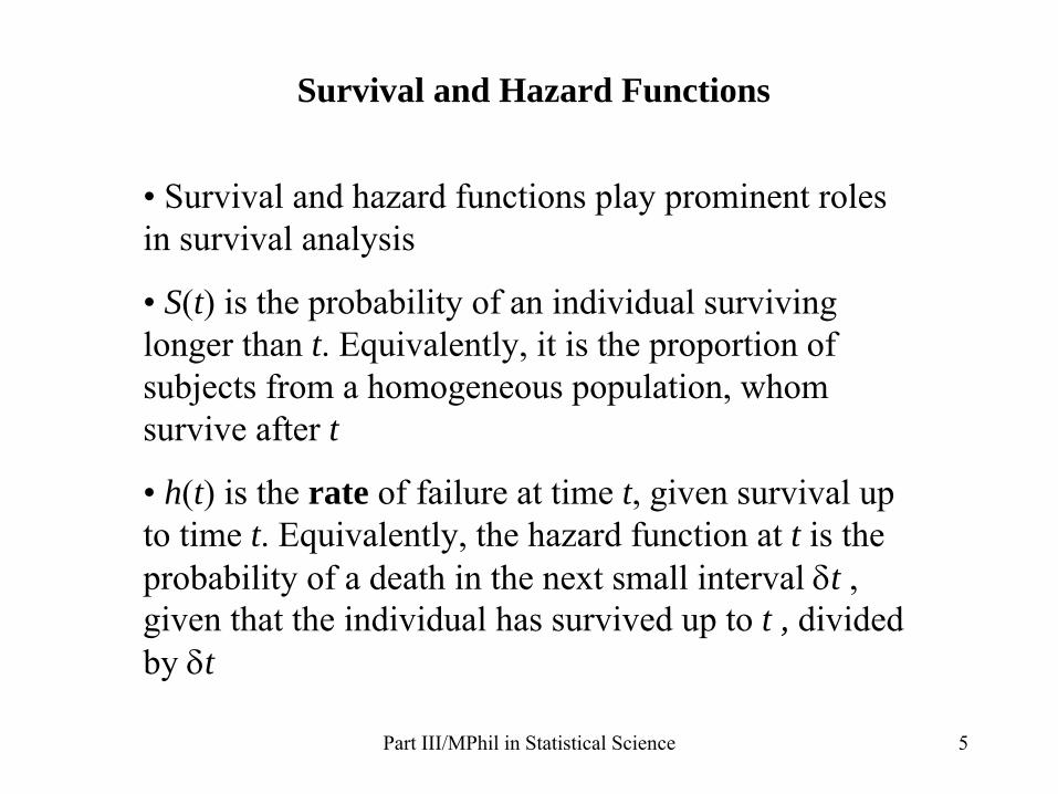
Survival and Hazard Functions

•

Survival and hazard functions play prominent roles in survival analysis

•

S(t) is the probability of an individual surviving longer than t. Equivalently, it is the proportion of subjects from a homogeneous population, whom survive after t

•

h(t) is the rate of failure at time t, given survival up to time t. Equivalently, the hazard function at t is the probability of a death in the next small interval δt , given that the individual has survived up to t , divided by δt


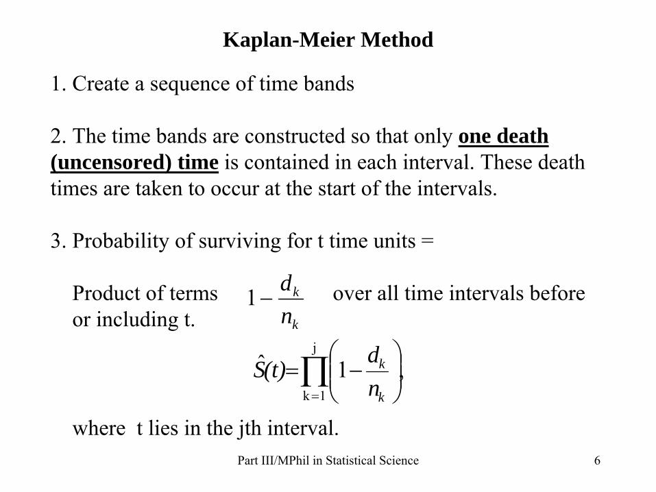
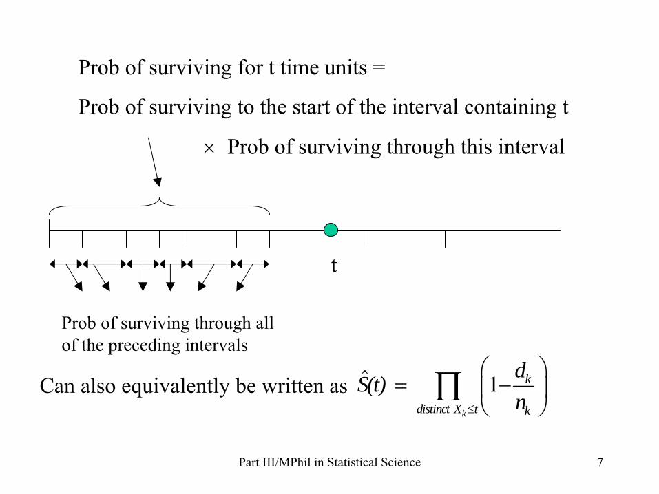
1. Create a sequence of time bands

2. The time bands are constructed so that only one death (uncensored) time is contained in each interval. These death times are taken to occur at the start of the intervals.

3. Probability of surviving for t time units =

Product of terms over all time intervals

before

or including t. k

k

nd

−1

,1 ˆj

1 k ∏=

⎟⎟⎠

⎞⎜⎜⎝

⎛−=

k

k

nd(t)S

where t lies in the jth

interval.

Kaplan-Meier Method


t

Prob

of surviving for t time units =

Prob

of surviving to the start of the interval containing t

×

Prob

of surviving through this interval

Prob

of surviving through all of the preceding intervals

Can also equivalently be written as

ˆ 1k

k

distinct X t k

dS(t)n≤

⎛ ⎞= −⎜ ⎟

⎝ ⎠∏


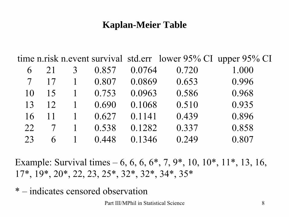
time n.risk n.event survival std.err lower 95% CI upper 95% CI 6 21 3 0.857 0.0764 0.720 1.0007 17 1 0.807 0.0869 0.653 0.99610 15 1 0.753 0.0963 0.586 0.96813 12 1 0.690 0.1068 0.510 0.93516 11 1 0.627 0.1141 0.439 0.89622 7 1 0.538 0.1282 0.337 0.85823 6 1 0.448 0.1346 0.249 0.807

Example: Survival times –

6, 6, 6, 6*, 7, 9*, 10, 10*, 11*, 13, 16, 17*, 19*, 20*, 22, 23, 25*, 32*, 32*, 34*, 35*

* –

indicates censored observation

Kaplan-Meier Table


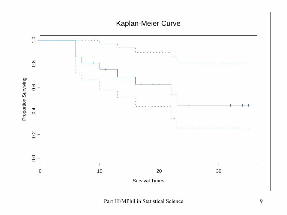
Survival Times

Pro

porti

on S

urvi

ving

0 10 20 30

0.0

0.2

0.4

0.6

0.8

1.0

Kaplan-Meier Curve


• K-M curve is the best description of the data

• Reading of the curve is straightforward

Example: Obtaining the median survival time (time beyond which 50% of the subjects in the study are expected to survive)

• K-M curves show the pattern of mortality over time

•

Not so good on details -

Overall pattern more enlightening and reliable

• Tendency to be drawn to the right-hand side of curve

• Place confidence bands around the curve


Testing Survival Data

•

In many studies (e.g. clinical trials), more than one group of subjects are under investigation

•

Interest now lies in comparing the survival experiences of these different groups

•

Example: 2 drugs -

Which of the two drugs is more effective in prolonging the lives of patients with small cell lung cancer?


•

We could try to answer this question after the study is completed by plotting the K-M curve for each group on the same graph and then assess visually

•

This may be informative and it is nonetheless good practice to plot the curves initially

•

However comparing K-M curves visually does not allow us to say, with confidence, if there is a true difference in survival experiences between the groups

•

The difference observed could be due to chance variation

•

Statistical test required to decide (formally) if there is evidence of a true difference


•

Note that it is not good practice to compare survival curves at a particular time point

• Why?


Log-Rank Test

•

Log-rank test used for comparing the survival differences between groups

•

Non-parametric test

•

Most powerful for non-overlapping survival curves

• Takes account of the whole range


•

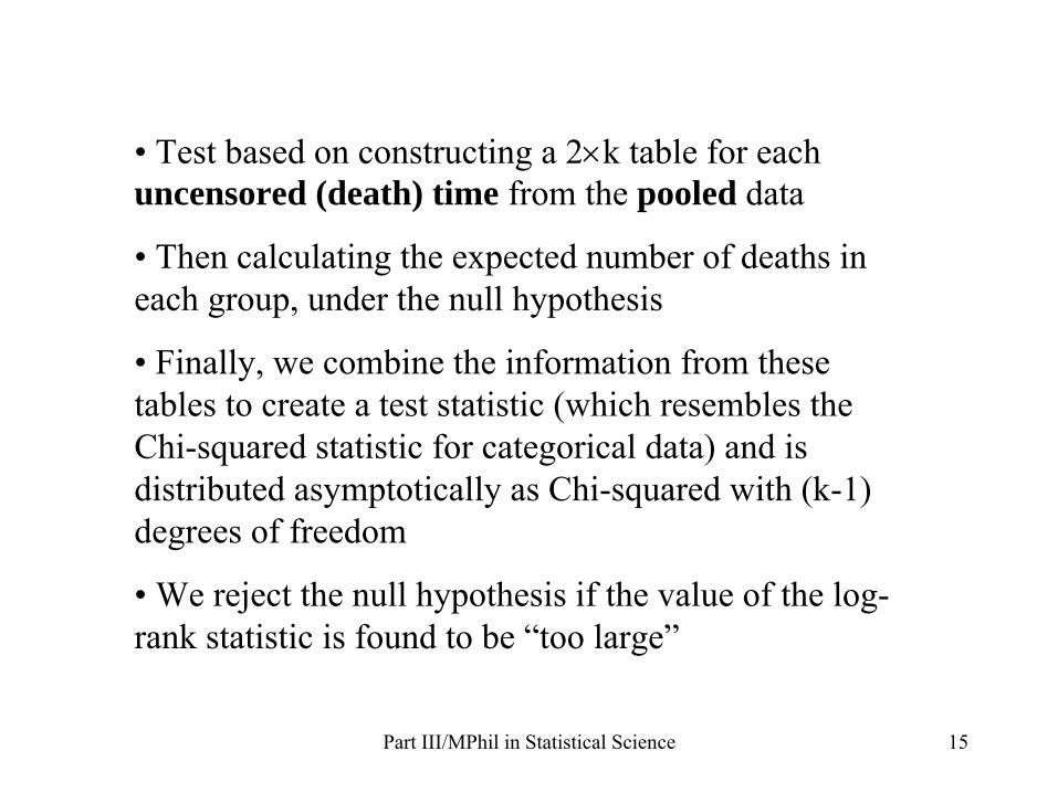
Test based on constructing a 2×k table for each uncensored (death) time from the

pooled data

•

Then calculating the expected number of deaths in each group, under the null hypothesis

•

Finally, we combine the information from these tables to create a test statistic (which resembles the Chi-squared statistic for categorical data) and is distributed asymptotically as Chi-squared with (k-1) degrees of freedom

•

We reject the null hypothesis if the value of the log- rank statistic is found to be “too large”


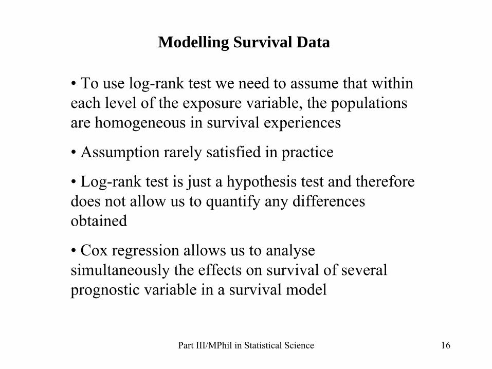
Modelling Survival Data

•

To use log-rank test we need to assume that within each level of the exposure variable, the populations are homogeneous in survival experiences

• Assumption rarely satisfied in practice

•

Log-rank test is just a hypothesis test and therefore does not allow us to quantify any differences obtained

•

Cox regression allows us to analyse simultaneously the effects on survival of several prognostic variable in a survival model


•

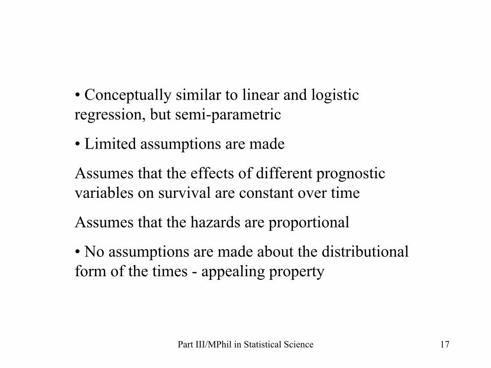
Conceptually similar to linear and logistic regression, but semi-parametric

• Limited assumptions are made

Assumes that the effects of different prognostic variables on survival are constant over time

Assumes that the hazards are proportional

•

No assumptions are made about the distributional form of the times -

appealing property


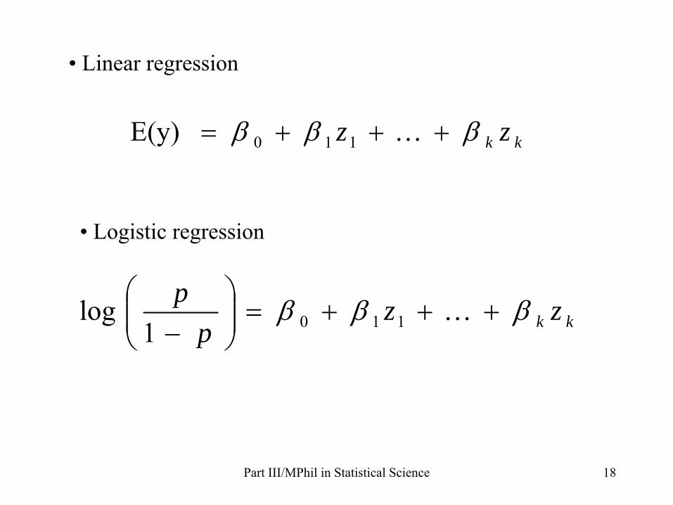
• Linear regression

kk zz βββ +++= …110E(y)

• Logistic regression

kk zzp

p βββ +++=⎟⎟⎠

⎞⎜⎜⎝

⎛−

…1101log


• Cox regression

)exp((t)hh(t) 110 kk zz ββ ++= …

baseline hazard

h(t) = h0

(t), when z1

= z2

= …

= zk

= 0


•

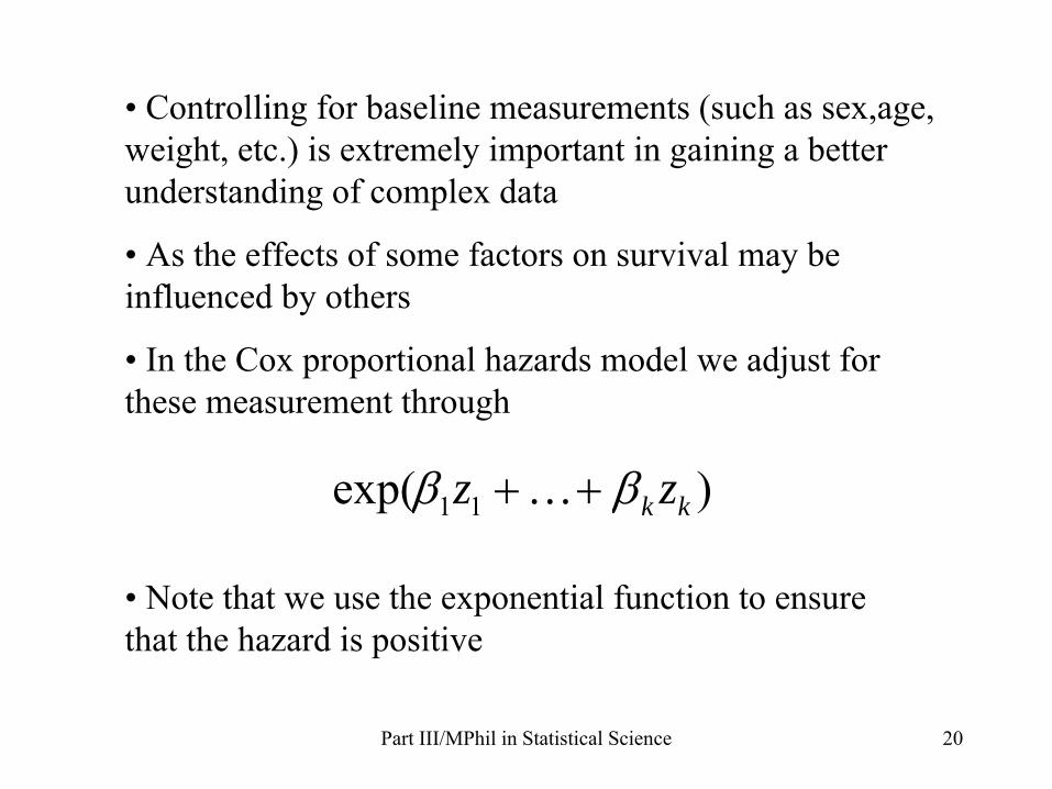
Controlling for baseline measurements (such as sex,age, weight, etc.) is extremely important in gaining a better understanding of complex data

•

As the effects of some factors on survival may be influenced by others

•

In the Cox proportional hazards model we adjust for these measurement through

)exp( 11 kk zz ββ ++…

•

Note that we use the exponential function to ensure that the hazard is positive


•

The interpreting of the parameter estimates in the Cox model is done in the same way as in logistic regression.

• We have hazard ratios instead of odds ratios


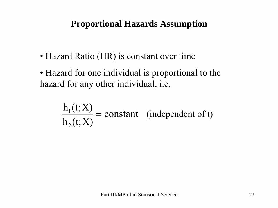
Proportional Hazards Assumption

• Hazard Ratio (HR) is constant over time

•

Hazard for one individual is proportional to the hazard for any other individual, i.e.

constantX)(t;hX)(t;h

2

1 = (independent of t)


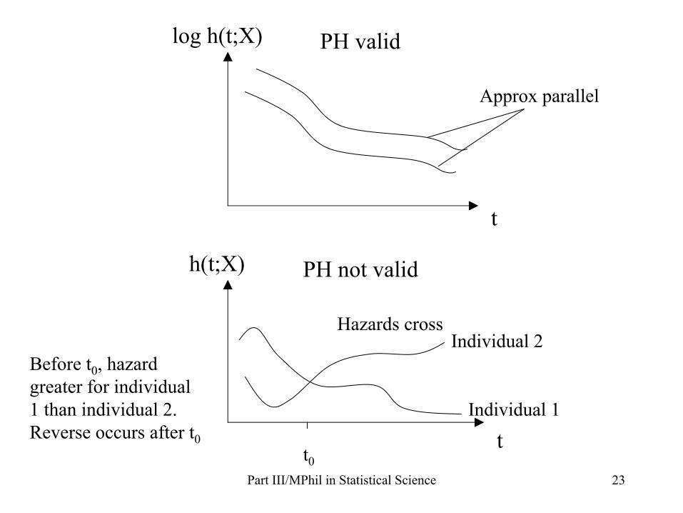
Approx parallel

log h(t;X)

t

PH valid

Hazards crossIndividual 2

Individual 1

PH not valid

t0

Before t0

, hazard greater for individual 1 than individual 2. Reverse occurs after t0

h(t;X)

t


•

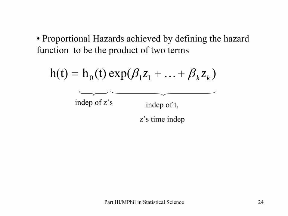
Proportional Hazards achieved by defining the hazard function to be the product of two terms

)exp( (t)hh(t) 110 kk zz ββ ++= …

indep

of z’s indep

of t,

z’s

time indep


Comments

•

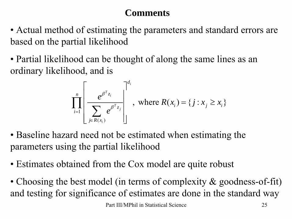
Actual method of estimating the parameters and standard errors are based on the partial likelihood

•

Partial likelihood can be thought of along the same lines as an ordinary likelihood, and is

•

Baseline hazard need not be estimated when estimating the parameters using the partial likelihood

• Estimates obtained from the Cox model are quite robust

•

Choosing the best model (in terms of complexity & goodness-of-fit) and testing for significance of estimates are done in the standard way

1

( )

, where ( ) { : }

i

Ti

Tj

i

d

zn

i j izi

j R x

e R x j x xe

β

β=

∈

⎡ ⎤⎢ ⎥

= ≥⎢ ⎥⎢ ⎥⎢ ⎥⎣ ⎦

∏∑


Diagnostics

• Checking the PH assumption is crucial

•

Valid interpretation of estimates rely on the PH assumption being satisfied

• We discuss two methods of assessing the PH assumption

•

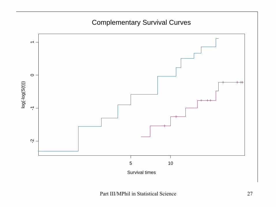
Graphical Approach -

Plot log(-logS(t)) curves for each level of the variable of interest, where S(t) can either be the K-M curve or the adjusted survival curve (i.e. adjusted for other covariates which satisfy the PH assumption)

•

Continuous variables need to be categorised -

Recommend creating small number of equal size categories

•

Parallel complementary curves indicate that the PH assumption is satisfied


Survival times

log(

-log(

S(t)

))

5 10

-2-1

01

Complementary Survival Curves


•

Analytical Approach -

Based on assessing whether the re-scaled Schoenfeld

residuals are correlated with some

transformation of time (e.g. K-M or Rank).

• Null hypothesis is that the PH assumption is valid

•

Therefore reject PH if there is an association between the re-scaled Schoenfeld

residuals and transformation of

time


•

When PH assumption is not valid for a particular variable, we include that variable into the Cox model as a stratifying variable

•

That is we assume different baseline hazards for each level of this variable

•

But we assume that the effects of the other variables are the same between different strata

•

To allow for different effects of some of the other variables in different strata, we can include an interaction between the stratifying variables and these variables

• Further extensions are possible but are not discussed here


Selection and Sampling Schemes

•

Up to now, restricted attention to right censoring•

Other forms of restriction on observation are possible–

Left censoring and truncation (right and left)

•

Left censoring occurs when the true survival time is less than the actual observed time (e.g. recurrence of leukaemia)

•

Truncation arises when individuals may be observed only within a certain observation window (SL , SR

). •

Subjects whose time-to-event is not in this window is not observed and no information on those subjects are available

•

Right truncation arises when SL

=0. Under observation only if true survival time less than SR

.•

Examples: –

Distance of stars from earth

–

Retrospective studies of AIDS


•

Left truncation arises when subjects with a time-to-event less than some threshold, SL

, are not observed at all.

•

Individuals come under observation only some known time after the natural/defined time origin of the event under study

• SR

=∞

• Different from left censoring where partial information is available

• Examples: − Diameters of microscopic particles

−

Disease studies in which patients come under observation at entry to clinic and possibly not from the relevant time origin (diagnosis or birth)


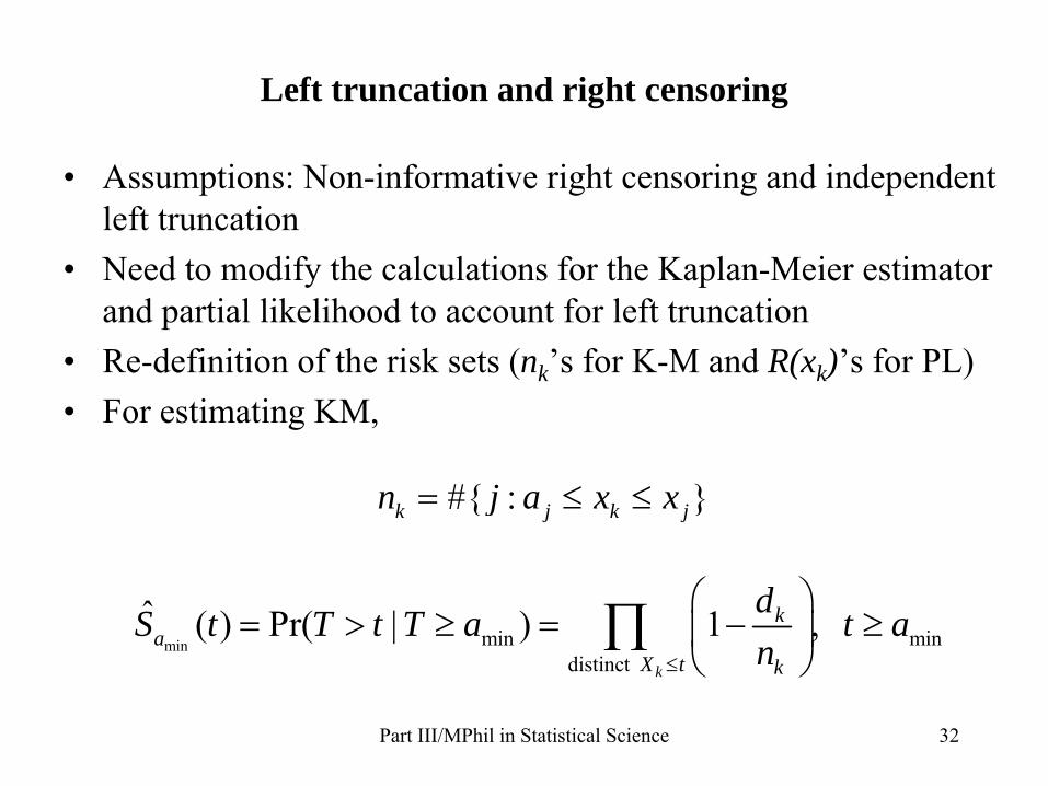
Left truncation and right censoring

•

Assumptions: Non-informative right censoring and independent left truncation

•

Need to modify the calculations for the Kaplan-Meier estimator and partial likelihood to account for left truncation

•

Re-definition of the risk sets (nk ’s

for K-M and R(xk )’s

for PL)•

For estimating KM,

#{ : }k j k jn j a x x= ≤ ≤

min min mindistinct

ˆ ( ) Pr( | ) 1 , k

ka

X t k

dS t T t T a t an≤

⎛ ⎞= > ≥ = − ≥⎜ ⎟

⎝ ⎠∏


•

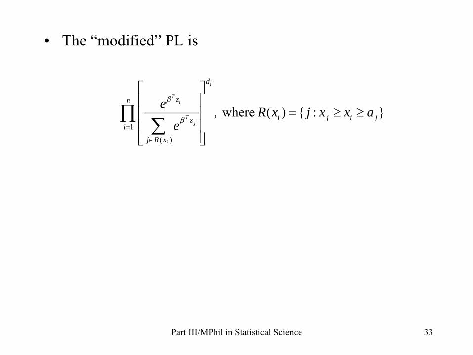
The “modified”

PL is

1

( )

, where ( ) { : }

i

Ti

Tj

i

d

zn

i j i jzi

j R x

e R x j x x ae

β

β=

∈

⎡ ⎤⎢ ⎥

= ≥ ≥⎢ ⎥⎢ ⎥⎢ ⎥⎣ ⎦

∏∑

Documents

SURVIVAL DATA ANALYSIS - MRC Biostatistics Unit · Survival and Hazard Functions • Survival and hazard functions play prominent roles in survival analysis • S (t) is the probability