Embed Size (px)
Citation preview

Survival Analysis of Bank Loans andCredit Risk Prognosis
School of Statistics and Actuarial Science
Submitted in fulfilment of the degree ofMaster of Science Mathematical Statistics
BY
Mercy Marimo506044
Supervisor
C Chimedza
April 12, 2015

Contents
1 Introduction 11.1 Why Survival Analysis? . . . . . . . . . . . . . . . . . . . . . . . . 21.2 Background of Study . . . . . . . . . . . . . . . . . . . . . . . . . . 3
1.2.1 Overview of the Basel Accord . . . . . . . . . . . . . . . . . 51.2.2 Definition of Default . . . . . . . . . . . . . . . . . . . . . . 61.2.3 Definition of Early Settlement . . . . . . . . . . . . . . . . . 6
1.3 Motivation . . . . . . . . . . . . . . . . . . . . . . . . . . . . . . . . 61.4 Aims and Objectives . . . . . . . . . . . . . . . . . . . . . . . . . . 81.5 Research Data . . . . . . . . . . . . . . . . . . . . . . . . . . . . . . 81.6 Data Source . . . . . . . . . . . . . . . . . . . . . . . . . . . . . . . 91.7 Limitations of Study . . . . . . . . . . . . . . . . . . . . . . . . . . 91.8 Summary . . . . . . . . . . . . . . . . . . . . . . . . . . . . . . . . 10
2 Literature Review 112.1 Introduction . . . . . . . . . . . . . . . . . . . . . . . . . . . . . . . 112.2 Background to Credit Scoring . . . . . . . . . . . . . . . . . . . . . 122.3 Logistic Regression . . . . . . . . . . . . . . . . . . . . . . . . . . . 152.4 Survival Analysis . . . . . . . . . . . . . . . . . . . . . . . . . . . . 172.5 Theoretical Review of Survival Analysis . . . . . . . . . . . . . . . . 182.6 Censoring . . . . . . . . . . . . . . . . . . . . . . . . . . . . . . . . 212.7 The Empirical Survivor Function . . . . . . . . . . . . . . . . . . . . 232.8 The Kaplan Meier Survival Estimator . . . . . . . . . . . . . . . . . 242.9 The Cox Proportional Hazards Regression Model . . . . . . . . . . . 26
2.9.1 Maximum Likelihood Estimation of the Cox Regression Model 28
CONTENTS ii
2.9.2 Tied Event Times in Cox PH Regression . . . . . . . . . . . . 282.9.3 Computation of the Hazard Ratio . . . . . . . . . . . . . . . 292.9.4 The Cox Proportional Hazards Assumption . . . . . . . . . . 302.9.5 Assessment of the Cox Proportional Hazards Assumption . . 31
2.10 Model Building Process . . . . . . . . . . . . . . . . . . . . . . . . . 332.10.1 Exploratory Data Analysis . . . . . . . . . . . . . . . . . . . 332.10.2 Univariate Data Analysis . . . . . . . . . . . . . . . . . . . . 342.10.3 Multivariate Data Analysis . . . . . . . . . . . . . . . . . . . 362.10.4 Goodness of Fit Measures . . . . . . . . . . . . . . . . . . . 362.10.5 Assessment of Model Performance . . . . . . . . . . . . . . 38
2.11 Competing Risks Survival Analysis . . . . . . . . . . . . . . . . . . 382.11.1 The Cause Specific Approach . . . . . . . . . . . . . . . . . 392.11.2 The Cumulative Incidence Curve . . . . . . . . . . . . . . . . 40
2.12 Parametric Models of Survival . . . . . . . . . . . . . . . . . . . . . 412.12.1 The Weibull Distribution . . . . . . . . . . . . . . . . . . . . 422.12.2 The Exponential Distribution . . . . . . . . . . . . . . . . . . 422.12.3 The Log-logistic Distribution . . . . . . . . . . . . . . . . . 43
2.13 Mixture Models of Survival . . . . . . . . . . . . . . . . . . . . . . . 432.13.1 The Proportional Hazards Mixture Model . . . . . . . . . . . 44
2.14 Conclusion . . . . . . . . . . . . . . . . . . . . . . . . . . . . . . . 44
3 Methodology 463.1 Introduction . . . . . . . . . . . . . . . . . . . . . . . . . . . . . . . 463.2 Data . . . . . . . . . . . . . . . . . . . . . . . . . . . . . . . . . . . 463.3 Exploratory Data Analysis . . . . . . . . . . . . . . . . . . . . . . . 493.4 Model Building . . . . . . . . . . . . . . . . . . . . . . . . . . . . . 49
3.4.1 Cox Regression Models . . . . . . . . . . . . . . . . . . . . 493.4.2 Logistic Regression Models . . . . . . . . . . . . . . . . . . 513.4.3 Model Assessment . . . . . . . . . . . . . . . . . . . . . . . 51

CONTENTS iii
4 Model Development 524.1 Introduction . . . . . . . . . . . . . . . . . . . . . . . . . . . . . . . 524.2 A Look at the Vehicle Brands on Book . . . . . . . . . . . . . . . . . 534.3 Model Building Process Flow . . . . . . . . . . . . . . . . . . . . . . 554.4 Data Extraction and Preparation . . . . . . . . . . . . . . . . . . . . 56
4.4.1 Definition of Events . . . . . . . . . . . . . . . . . . . . . . 574.4.2 Outcome Period Analysis . . . . . . . . . . . . . . . . . . . 574.4.3 Sampling Approach . . . . . . . . . . . . . . . . . . . . . . 58
4.5 Covariate Selection . . . . . . . . . . . . . . . . . . . . . . . . . . . 594.5.1 Covariate Binning Process . . . . . . . . . . . . . . . . . . . 614.5.2 Default Model Univariate Analysis . . . . . . . . . . . . . . 634.5.3 Default Model Multivariate Analysis - Cox Regression . . . . 664.5.4 Early Settlement Model Univariate Analysis . . . . . . . . . . 684.5.5 Early Settlement Model Multivariate Analysis - Cox Regression 70
4.6 Summary . . . . . . . . . . . . . . . . . . . . . . . . . . . . . . . . 71
5 Results and Analysis 735.1 Introduction . . . . . . . . . . . . . . . . . . . . . . . . . . . . . . . 735.2 Model Fitting . . . . . . . . . . . . . . . . . . . . . . . . . . . . . . 735.3 Logistic Regression . . . . . . . . . . . . . . . . . . . . . . . . . . . 74
5.3.1 Default Model Multivariate Analysis - Logistic Regression . . 745.3.2 Default Model - Logistic Regression . . . . . . . . . . . . . . 765.3.3 Goodness of fit Statistics - Default Logistic Model . . . . . . 775.3.4 Early Settlement Model Multivariate Analysis - Logistic Re-
gression . . . . . . . . . . . . . . . . . . . . . . . . . . . . . 805.3.5 Early Settlement Logistic Regression Model . . . . . . . . . 825.3.6 Goodness of fit Statistics - ES Logistic Model . . . . . . . . . 84
5.4 Cox PH Regression . . . . . . . . . . . . . . . . . . . . . . . . . . . 865.4.1 Long Term Survivors . . . . . . . . . . . . . . . . . . . . . . 865.4.2 Analysis of The Hazard Functions . . . . . . . . . . . . . . . 87
5.4.2.1 Default Event . . . . . . . . . . . . . . . . . . . . 875.4.2.2 Early Settlement Event . . . . . . . . . . . . . . . 88
5.4.3 Default Model . . . . . . . . . . . . . . . . . . . . . . . . . 89
CONTENTS iv
5.4.4 Intuitiveness of Signs - Default Cox PH Model . . . . . . . . 915.4.5 Goodness of Fit Statistics - Cox PH Default Model . . . . . . 935.4.6 Early Settlement Model . . . . . . . . . . . . . . . . . . . . 945.4.7 Intuitiveness of Signs - Early Settlement Model . . . . . . . . 95
5.5 Goodness of Fit Statistics - ES Cox PH Model . . . . . . . . . . . . . 975.6 Model Comparison and Validation Metrics . . . . . . . . . . . . . . . 98
5.6.1 Rank Ordering Metrics . . . . . . . . . . . . . . . . . . . . . 985.6.2 Model Gini Statistics . . . . . . . . . . . . . . . . . . . . . . 985.6.3 The ROC Curves . . . . . . . . . . . . . . . . . . . . . . . . 99
5.7 Credit Risk Model Standards . . . . . . . . . . . . . . . . . . . . . . 1015.8 Summary . . . . . . . . . . . . . . . . . . . . . . . . . . . . . . . . 102
6 Summary, Conclusion and Recommendations 1036.1 Introduction . . . . . . . . . . . . . . . . . . . . . . . . . . . . . . . 1036.2 Summary . . . . . . . . . . . . . . . . . . . . . . . . . . . . . . . . 1046.3 Conclusion . . . . . . . . . . . . . . . . . . . . . . . . . . . . . . . 1056.4 Recommendations . . . . . . . . . . . . . . . . . . . . . . . . . . . . 106
References 109
Appendix A Univariate Assessment 112A.1 Default Model - Initial PH Assessment . . . . . . . . . . . . . . . . . 112A.2 Default Model - Final PH, Event Rate, Population Stability and WoE
Assessment . . . . . . . . . . . . . . . . . . . . . . . . . . . . . . . 114A.3 Early Settlement Model - Initial PH Assessment . . . . . . . . . . . . 117A.4 ES Model - Final PH, Event Rate, Population Stability and WoE As-
sessment . . . . . . . . . . . . . . . . . . . . . . . . . . . . . . . . . 119
Appendix B The SAS R© Code 122B.1 Data Extraction . . . . . . . . . . . . . . . . . . . . . . . . . . . . . 122B.2 Data Preparation . . . . . . . . . . . . . . . . . . . . . . . . . . . . 124B.3 Derivation of Critical Fields . . . . . . . . . . . . . . . . . . . . . . 129B.4 Covariate Selection . . . . . . . . . . . . . . . . . . . . . . . . . . . 131

CONTENTS v
B.5 Univariate Analysis . . . . . . . . . . . . . . . . . . . . . . . . . . . 136B.6 Multivariate Analysis . . . . . . . . . . . . . . . . . . . . . . . . . . 181B.7 Cox PH regression . . . . . . . . . . . . . . . . . . . . . . . . . . . 189B.8 CIC . . . . . . . . . . . . . . . . . . . . . . . . . . . . . . . . . . . 191B.9 Logistic Regression . . . . . . . . . . . . . . . . . . . . . . . . . . . 195B.10 Model Assessment and Comparisons . . . . . . . . . . . . . . . . . . 197

List of Figures
1.1 Biplot of Vehicle Brands . . . . . . . . . . . . . . . . . . . . . . . . 4
2.1 Censoring . . . . . . . . . . . . . . . . . . . . . . . . . . . . . . . . 222.2 Empirical Survival Curve . . . . . . . . . . . . . . . . . . . . . . . . 232.3 Comparison of Survivor Curves . . . . . . . . . . . . . . . . . . . . 25
4.1 Brands on Book . . . . . . . . . . . . . . . . . . . . . . . . . . . . . 554.2 Outcome Period Analysis . . . . . . . . . . . . . . . . . . . . . . . . 584.3 Binning Process . . . . . . . . . . . . . . . . . . . . . . . . . . . . . 624.4 PH Assessment - Default Model . . . . . . . . . . . . . . . . . . . . 644.5 Univarite Assessment Plots - Default Model . . . . . . . . . . . . . . 654.6 Population Stability . . . . . . . . . . . . . . . . . . . . . . . . . . . 664.7 Multivariate Analysis - Default Model . . . . . . . . . . . . . . . . . 674.8 Multivariate Analysis - Early Settlement Model . . . . . . . . . . . . 71
5.1 Default Model Selection Criteria . . . . . . . . . . . . . . . . . . . . 755.2 Accuracy Plots Default Model . . . . . . . . . . . . . . . . . . . . . 805.3 Early Settlement Model Selection Criteria . . . . . . . . . . . . . . . 815.4 Accuracy Plots Early Settlement Model . . . . . . . . . . . . . . . . 855.5 Kaplain Meier Survival Curve . . . . . . . . . . . . . . . . . . . . . 875.6 Default Event - Hazard Function . . . . . . . . . . . . . . . . . . . . 885.7 Early Settlement Event - Hazard Function . . . . . . . . . . . . . . . 895.8 Accuracy Plots Default Cox Model . . . . . . . . . . . . . . . . . . . 935.9 Accuracy Plots Early Settlement Cox Model . . . . . . . . . . . . . . 975.10 ROC Curves . . . . . . . . . . . . . . . . . . . . . . . . . . . . . . . 99

LIST OF FIGURES vii
A.1 Initial PH Assessment - Default Model . . . . . . . . . . . . . . . . . 113A.2 Univariate Assessment - Default Model . . . . . . . . . . . . . . . . 116A.3 Initial PH Assessment - ES Model . . . . . . . . . . . . . . . . . . . 118A.4 Univariate Assessment - ES Model . . . . . . . . . . . . . . . . . . . 121
List of Tables
3.1 Standard Variables . . . . . . . . . . . . . . . . . . . . . . . . . . . 473.2 Customer and Vehicle Specific Covariates . . . . . . . . . . . . . . . 48
4.1 Brands on Book . . . . . . . . . . . . . . . . . . . . . . . . . . . . . 544.2 Model Building Process Flow . . . . . . . . . . . . . . . . . . . . . . 564.3 Sample Selection . . . . . . . . . . . . . . . . . . . . . . . . . . . . 594.4 Selection of Numerical Covariates . . . . . . . . . . . . . . . . . . . 604.5 Selection of Categorical Covariates . . . . . . . . . . . . . . . . . . . 614.6 Binning Process . . . . . . . . . . . . . . . . . . . . . . . . . . . . . 624.7 Default Model - Univariate Gini Statistics . . . . . . . . . . . . . . . 634.8 Final Covariates - Default Model . . . . . . . . . . . . . . . . . . . . 684.9 Early Settlement Model - Univariate Gini Statistics . . . . . . . . . . 694.10 Final Covariates - Early Settlement Model . . . . . . . . . . . . . . . 71
5.1 Baseline Population . . . . . . . . . . . . . . . . . . . . . . . . . . . 745.2 Variable Importance - Default Model . . . . . . . . . . . . . . . . . . 755.3 Logistic Stepwise Regression - Default Model . . . . . . . . . . . . . 765.4 Logistic Regression - Default Model Estimates . . . . . . . . . . . . 775.5 Intuitiveness of Signs of the Default Model - Logistic Regression . . . 785.6 The Hosmer and Lemeshow Partition - Default Model . . . . . . . . . 795.7 Variable Importance - ES Model . . . . . . . . . . . . . . . . . . . . 815.8 Logistic Regression - ES Model Estimates . . . . . . . . . . . . . . . 825.9 Intuitiveness of Signs of the Early Settlement Model - Logistic Regres-
sion . . . . . . . . . . . . . . . . . . . . . . . . . . . . . . . . . . . 835.10 The Hosmer and Lemeshow Partition - ES Logistic Model . . . . . . 84

LIST OF TABLES ix
5.11 Global Null Hypothesis . . . . . . . . . . . . . . . . . . . . . . . . . 895.12 Type 3 Tests . . . . . . . . . . . . . . . . . . . . . . . . . . . . . . . 905.13 Cox PH - Default Model Estimates . . . . . . . . . . . . . . . . . . . 905.14 Intuitiveness of Signs of the Default Model . . . . . . . . . . . . . . 925.15 Globall Null Hypothesis . . . . . . . . . . . . . . . . . . . . . . . . 945.16 Type 3 Tests . . . . . . . . . . . . . . . . . . . . . . . . . . . . . . . 945.17 Cox PH - Early Settlement Model Estimates . . . . . . . . . . . . . . 955.18 Intuitiveness of Signs of the Early Settlement Model . . . . . . . . . 965.19 Model Gini Statistics . . . . . . . . . . . . . . . . . . . . . . . . . . 985.20 Area under ROC Curves . . . . . . . . . . . . . . . . . . . . . . . . 100

Dedication
I would like to dedicate this project to God Almighty for having this project as part ofhis grand plan for my life, and to my parents, Mr. Josephat and Mrs. Cecilia Dzikitiwho always believed in me since my childhood. My daughter Kudzai Munemo, thankyou for being patient with me throughout my studies. For this reason, I dedicate thisproject to you.

Acknowledgements
My project was successfully concluded due to the support of many people to whomI give my heartfelt gratitude. Firstly, I would like to thank my only daughter KudzaiMunemo for her understanding, love, kindness and patience throughout my studies.Special thanks to my supervisor, Mr. Charles Chimedza who offered me tremendousencouragement, guidance and support. I give special appreciation to my home af-fairs agent Mr. Brehme Nefale of Nefale Holdings for processing my documentationtimeously and unreservedly, to enable my registration with the University of the Wit-watersrand. Furthermore, I give thanks to the school of Statistics and Actuarial Sciencefor according me another chance to prove my ability and strength in the MathematicalStatistics domain. Last but not least, I extend many thanks to the financial institution Iwork for, one of the largest financial institutions in South Africa, for the much neededlifetime data, the time and platform to work on, amongst other resources provided.

Abstract
Standard survival analysis methods model lifetime data where cohorts are tracked fromthe point of origin, until the occurrence of an event. If more than one event occurs, aspecial model is chosen to handle competing risks. Moreover, if the events are definedsuch that most subjects are not susceptible to the event(s) of interest, standard survivalmethods may not be appropriate. This project is an application of survival analysis in aconsumer credit context. The data used in this study was obtained from a major SouthAfrican financial institution covering a five year observation period from April 2009 toMarch 2014. The aim of the project was to follow up on cohorts from the point wherevehicle finance loans originated to either default or early settlement events and comparesurvival and logistic modeling methodologies. As evidenced by the empirical KaplainMeier survival curve, the data typically had long term survivors with heavy censoringas at March 2014. Cause specific Cox regression models were fitted and an adjustmentwas made for each model, to accommodate a proportion p of long term survivors. Thecorresponding Cumulative Incidence Curves were calculated per model, to determineprobabilities at a fixed horizon of 48 months. Given the complexity of the consumercredit lifetime data at hand, we investigated how logistic regression methods wouldcompare. Logistic regression models were fitted per event type. The models wereassessed for goodness of fit. Their ability to differentiate risk were determined usingthe model Gini Statistics. Model assessment results were satisfactory. Methodologieswere compared for each event type using Receiver Operating Characteristic curvesand area under the curves. The Results show that survival methods perform better thanlogistic regression methods when modelling lifetime data in the presence of competingrisks and long term survivors.

LIST OF TABLES 4
List of Abbreviations
Term Description
AFT Accelerated Failure Time
AIC Akaike Information Criteria
BCBS Basel Committee on Banking Supervision
CIC Cumulative Incidence Curve
DLR Dichotomous Logistic Regression
EAD Exposure at Default
EDA Exploratory Data Analysis
ECOA Equal Credit Opportunity Act
ES Early Settlement
ESF Empirical Survival Function
GS Gini Statistic
HR Hazard Ratio
IV Information Value
KM Kaplan Meier
LGD Loss Given Default
LMH Log-rank Mantel-Haenszel
LR Logistic Regression
OLS Ordinary Least Squares
PD Probability of Default
PH Proportional Hazards
ROC Receiver Operating Characteristic
SBC Schwarz Bayesian Criterion
VIF Variance Inflation Factor
WoE Weight of Evidence

Chapter 1
Introduction
Survival analysis is a statistical data analysis technique, designed to analyse the amountof time it takes for an event to occur, over an observation period. The technique modelslifetime data. The units of time in survival analysis range from days, weeks, months,years and even decades from the beginning of follow up till an event occurs or until ob-servation ceases (censorship). Survival analysis originated in the biomedical researchdiscipline where the event of interest was death of biological organisms, (Smith andSmith, 2000). Nowadays, the event refers to various other aspects depending on thedomain of study and its context. In the social sciences, the event may refer to a changein social status, for example marital status. In engineering, the event may be decom-missioning of machines. Natural disasters may be taken as the event in geosciencesand the onset of a disease is an event in Epidemiology. Where the event is a nega-tive experience, for example relapse or death in cancer patients, the event is usuallyreferred to as failure.
In this study, survival analysis is applied to consumer credit data, a case for a leadingSouth African banking institution. Consumer credit data is analogous to lifetime dataas it concerns the credit status of a cohort of customers with different loan repaymentbehaviours over a given observation period. A single money lending product offeringinstalment loans is considered in this case, whereby a customer repays the loan in in-stalments, on a monthly basis over a predetermined repayment period.

1.1 Why Survival Analysis? 2
We apply survival methodologies to the prediction of two mutually exclusive events,default and Early Settlement (ES). The occurrence of these two events over the ob-servation period impacts negatively on profitability. Lenders prefer a longer time todefault as the acquired interest will compensate for, or even exceed losses due to de-fault, (Stepanova and Thomas, 2002). In the consumer credit context, survival methodsresults can be used as input into the computation of credit risk parameters. These playa crucial role in risk management, and include the Probability of Default (PD), LossGiven Default (LGD) and Exposure at Default (EAD) models.
1.1 Why Survival Analysis?
Survival analysis is time to event analysis of lifetime data. It is applicable in any scien-tific domain of study where researchers are interested in measuring the likelihood of anevent and when it is likely to occur. Conventional statistical modelling techniques arenot compatible with the nature of survival data, since survival data is not strictly nor-
mally distributed and its format includes details of censoring. Censoring occurs whenthe survival time of some respondents is partly known, that is, the survival time is in-complete for some individual cases (Hubber and Patetta, 2013). Thus, survival datacannot be analyzed using the traditional statistical procedures such as linear regressionwhere the normality assumption is key and censoring is not accounted for. Accordingto Tableman (2008), prior to the survival analysis method, subjects with incompletedata were deleted before the analysis. Deletion of censored observations results in lossof valuable information and consequently underestimation or overestimation of param-eters of interest. Survival methods are believed to give more accurate estimates as theyaccommodate the censored data obtained throughout the observation period.
Survival methodology is appealing for its flexibility in the usage of parametric andsemi parametric models depending on the choice of the researcher and the underlyingnature of the data. Where semi parametric models are used, as often is the case, aminimum of assumptions is required to obtain the key features desired from survivaldata, these are the survival and hazard functions. Semi parametric methodologies of

1.2 Background of Study 3
survival analysis make no distributional assumption as to the appropriateness of theresponse variable, lifetime of bank loans in this case. This feature saves a lot on dataassessment, preparation and computational time. It is less computationally intensive inthe case of huge data sets where computer and software performance is key (Hubberand Patetta, 2013).
1.2 Background of Study
Vehicle Finance, which will be referred to as the “product” in this study, is mainly donethrough the mainstream banking system in South Africa. The product extends loansfor the purchase of motor vehicles. This study focuses on the retail end of the mar-ket which finances the purchase of light-delivery vehicles, taxis, agricultural vehicles,motorcycles, watercraft, caravans, and trailers. It finances among other retail speci-fications, self-employed persons, taxi finance, and small businesses. The InstalmentSale Agreement product is considered in this study. Financing terms range between12 and 72 months with/without a deposit depending on credit worthiness of individualcustomers at the time of application.
Figure 1.1 is a biplot constructed by the author based on a survey recently conductedon the South African automobile market concerning a sample of budget brands. Abiplot is a graphical display of multivariate data where rows and columns are depictedas points. It is analogous to a scatter plot in a bivariate scenario (Le Roux and Gardner,2005). It represents relationships and association among multiple variables. The biplotin Figure 1.1 depicts some factors which drive particular vehicle brands. The squaresin the plot represent vehicle brands offered on the South African market. The bulk ofthe bank loans in terms of volumes are associated with popular brands represented inthe biplot. The circles represent attributes. Each vehicle brand is mainly associatedwith attributes in close proximity to the respective square points.
According to the survey, Volkswagen offers powerful, high quality vehicles and cus-tomers readily recommend the brand. Nissan and Ford are environmentally friendly

1.2 Background of Study 4
vehicles and motorists feel confident with the brands. Toyota and Mazda are fuel effi-cient and they offer good after sales service plans. Honda and Renault offer modern ve-hicles with attractive styling, prestigious and exciting. Hyundai, Volkswagen and Kiamanufacture high quality and safe vehicles. Customers feel proud to be seen drivingvehicles from the Suzuki range. Opel, Nissan and Ford vehicles are environmentallyfriendly budget cars and customers feel confident when driving them.
Figure 1.1: Biplot of Vehicle Brands
In practise, budget vehicles are cheap, fuel efficient and they offer good after sales/serviceplans. These are in demand mainly by the lower end of the market and the vehiclessales move in high volumes. For most consumers, budget vehicles are mainly usedfor day to day chores owing to reasonably low maintenance costs. Manufacturers wellknown to produce budget vehicles include Toyota, Mazda, Opel and Chevrolet. Luxu-rious vehicles are often expensive and sales volumes account for a smaller percentage.

1.2 Background of Study 5
These are in demand by the upper end of the market. Customers in this category areusually driven by exciting, high quality, attractive styling, powerful and prestigiousvehicles.
Banks in South Africa play a very important role in financing vehicle purchases. Thebulk of recipients of vehicle loans are “good” customers as they repay the loans overthe agreed repayment period without impairments. However, it is inevitable to find“bad” customers within the system. This study focuses on the volume of bad cus-tomers and quantifies losses anticipated on such customers in a specified time interval.For compliance purposes and consistency with international standards, the two eventsanalysed in this study, default and ES are defined in line with the Basel Accord (de-fined below) and bank definitions respectively.
1.2.1 Overview of the Basel Accord
Following the messy banking system collapse in the 1970s, the G10 major westerneconomies agreed on bank supervison rules which regulates finance and banking in-ternationally. The rules are set by a committee that meets in Basel, a city in the north-western Switzerland, at the Bank for International Settlements. The Basel Committeeon Banking Supervision (BCBS) (2006) issues and maintains Basel Accords.
Basel Accords are a series of recommendations on banking laws and regulations setout to ensure that international banks maintain adequate capital to sustain themselvesduring the periods of economic strain. According to Cai and Wheale (2009), the firstaccord, ‘Basel I’ was reached around 1988. The improved ‘Basel II’ was issued in2004 and is currently in use. The Basel standards are not enforced by the Committee;however, countries that adopt the standards are expected to create and enforce regula-tions created from their specifications.
The South African banking community adopted the standards and this governs capitalmarkets and model building standards. Accordingly, this study follows descriptions bythe BCBS (2006) to define default. The definition of default is restated as follows:

1.3 Motivation 6
1.2.2 Definition of Default
A default is considered to have occurred with regard to a particular borrower wheneither or both of the two following events have taken place.
1. The bank considers that the obligor is unlikely to repay his/her credit obligationsto the bank in full.
2. The obligor is more than 90 days past the due date on any credit obligation tothe banking group.
1.2.3 Definition of Early Settlement
Early settlement refers to early closure of loan accounts. The customer “settles” theoutstanding amount ahead of the original repayment period. The reasons for early clo-sure of accounts differ from customer to customer. Some customers close accountsby switching to another lender. In South Africa, some customers upgrade to newlyreleased car models causing early closure of existing accounts and the opening of newaccounts. A completely new set of customer specific and vehicle specific applicationvariables are captured. As such, new accounts are treated separately from the old ac-count for the same individual.
Default and ES events impact negatively on the lender because they both cut out aproportion of anticipated interest.
1.3 Motivation
Conventional models of credit risk were often built on static variables obtained fromapplication data. Logistic Regression (LR) has been the cornerstone of credit models.It plays a very important role in building scorecards, which determine whether an ap-plicant should be granted a loan or not. The scorecards, coupled with capital models,PD, EAD and LGD serve as input into the pricing models to calculate the amount theapplicant qualifies for and the relevant interest rate at application.
1.3 Motivation 7
Even though LR methods have been in use for model building, Belloti and Crook(2007) showed that survival analysis methods are more competitive and often superiorto the LR approach. Survival methods use more information in model building thanLR. More information includes details of censoring as well as survival time of everysubject under study. Survival analysis techniques are applied in this study because ofthe existence of lifetime history of bank loans and censored observations in consumercredit data. Survival lifetime per account is the response variable.
Two events of interest are defined and considered simultaneously. These are defaultand ES. Analysis of more than one event in the same study is a variation of survivalanalysis known as competing risks analysis. A single customer can only experienceone of the events and not both or gets censored. In this case, censorship occurs whena customer neither defaults nor pays off early such that the event of interest is neverobserved (Stepanova and Thomas, 2002). Censored subjects in this case are “good”customers. Thus, while logistic regression indicates if a customer will experience anevent, leading to credit scoring, survival methods determine not only if, but also predictwhen, a customer will experience an event of interest (Banasik, Crook and Thomas,1999). Survival analysis is applicable to both credit and profit scoring.
The likelihood of default and ES is highly influenced by general economic conditionsthat are measured by time-varying macroeconomic variables such as earnings, all-shareprice index, unemployment index, interest rates and so on. Time-varying variablescannot readily be included in logistic regression models. Belloti and Crook (2007)conducted experiments to prove that the inclusion of macroeconomic variables usingsurvival methods gives statistically significant models and uplifts model predictive per-formance compared to models which exclude the macroeconomic variables. Survivalanalysis accommodates dynamic survival models by allowing for time-dependent vari-ables such as macroeconomic and behavioral variables. Inclusion of time-dependentvariables in survival methods is beyond the scope of this study due to data complexityin the consumer credit context.

1.4 Aims and Objectives 8
1.4 Aims and Objectives
The purpose of this study is to analyse competing risks in consumer credit data withtwo events of interest, default and ES. The specific objectives are as follows:
1. Perform a univariate analysis using the Gini Statistic (GS) for each candidatecovariate in order to identify and select variables capable of differentiating risk.
2. Conduct a multivariate analysis of the predictor variables, including correlationanalysis and the Variance Inflation Factor (VIF) to determine the statistical rela-tionships among them.
3. Use stepwise regression to select a combination of variables which strive to giveoptimum statistical power when used together in a model.
4. Fit the Cox regression model to the development data set for the default eventassuming early repayment as the censored event.
5. Fit the Cox regression model to the development data set for the early repaymentevent assuming default as the censored event.
6. For each model, assess the validity of the proportional hazards assumption.
7. Use the cause specific hazards as an intermediate step into the calculation of theCumulative Incidence Curve (CIC) for each model.
8. Fit a logistic regression model for each of the events.
9. Compare Cox regression and logistic regression based on estimating which loansare likely to default/pay off early in a fixed outcome period.
1.5 Research Data
This study explores a data set obtained in the consumer credit context. The analysislooks at facility level information, rather than at customer level. That means in theevent that a customers holds more than one account, this study treats each account sep-arately. The facility level rule is in line with the Basel Accord, “For retail exposures,

1.6 Data Source 9
the definition of default can be applied at the level of a particular facility, rather thanat the level of the obligor. As such, default by a borrower on one obligation does notrequire a bank to treat all other obligations to the banking group as defaulted”, BCBS(2006, page 101).
The data set will consist of all active accounts between 01 April 2009 and 31 March2014. Application and behavioural variables are provided per account in the data set.The repayment status is given per account per month under observation. A fixed work-out/outcome period will be determined and used in the calculation of forward lookingprobabilities. A workout period is the amount of time it takes for the bulk of accountsto be absorbed into the events of interest.
1.6 Data Source
This study utilises consumer credit data obtained from a leading South African finan-cial institution. The institution adopted standards outlined in the Basel Accord. Thisimplies that the data complies with the international standards and that the data is cred-ible for study purposes.
1.7 Limitations of Study
International legislation prevents the use of certain covariates such as gender and pop-ulation group in credit granting decisions (Hand and Henley, 1997). This is meant tocurb irrational prejudices. Classification is based solely on merit (past behaviour andcredit record of applicants). Such variables prohibited by the law will not be used ascovariates in this study.
The study considers customers whose loans were approved. No information is avail-able for rejected applicants and for customers who rejected the offer (in attrition).

1.8 Summary 10
1.8 Summary
Chapter one introduced the reader to the methodologies proposed for use in this disser-tation, the background of study, motivation, aims and objectives as well as limitationsof study. Survival analysis originated in biomedical research but in this case it is beingapplied to consumer credit data which is analogous to lifetime data as it concerns afollow up on the behaviour of cohorts over time. Survival analysis is believed to bea more appealing approach in studies involving lifetime data as compared to logisticregression. This study is aimed at investigating the notion and verify whether survivalanalysis outperforms logistic regression in the presence of competing risks which aredefault and ES.

Chapter 2
Literature Review
2.1 Introduction
This chapter features the history, development and redevelopment of credit scoringsystems spanning from the pre computer era to the current methodologies employedby financial institutions. Emphasis is placed on statistically sound approaches to mod-elling credit risk, possibilities, pitfalls and limitations of various techniques. Creditscoring systems have been redeveloped continuously to conform to the ever changingworld.
Of major importance motivating this report is the critical statistical analysis of bankloans, not only if, but when, customers will default. This section zooms into the ori-gins and progression of survival analysis techniques up to its application in modelsof credit. A theoretical review of survival analysis methods highlights the terminol-ogy and notation often used and describes relevant mathematical models applied. Anoverview of the features and theoretical properties of survivor curves is outlined aswell as statistical approaches used to compare survivor curves and to test significance.Variations of the modeling technique arise due to the purpose of study, the nature of theoutcome variable, the event(s) of interest and also the type of input variables availablefor the analysis.

2.2 Background to Credit Scoring 12
2.2 Background to Credit Scoring
The term credit refers to an amount of money loaned to a customer by a granter, whichmust be repaid, with interest, under agreed terms and conditions. Loans may be fixedterm, rolling or revolving, where loan amounts can be increased flexibly. Credit scor-
ing is the name used for customer’s classification into risk classes according to theirability to repay debt. Credit scores are usually estimated using the creditor’s historicdata under the presumption that the future is like the past. Prediction and modellingof the future is thus determined by the past historical information. The ability to offercredit by financial institutions has important profit implications while the ability to ob-tain credit by the customers has important quality of life implications (Jilek, 2008).
Prior to the computer age, credit granting decisions were based on subjective humanassessment in a process called judgemental methods. There was no legislation in placeto govern and control decisions made. According to Capon (1982), before the launchof the Equal Credit Opportunity Act (ECOA), passed in 1974, credit systems discrim-inated granting of loans based on gender and marital status. ECOA enforced equalopportunity in accessing loans by customers irrespective of gender and marital sta-tus. Judgemental methods of granting credit which involved individual judgement bya credit officer on a case to case basis were replaced by an automated way of makingcredit decisions, referred to as credit scoring. Not only banks adopted credit scoring,retailers, oil companies, travel and entertainment entities also utilised the credit scor-ing system.
Running concurrently to judgemental methods were numerical scoring systems, firstdeveloped in the mail order industry around 1930 (Capon, 1982). Certain characteris-tics were chosen for their ability to differentiate risk. Points were awarded to differentlevels of the characteristics. Decisions were based on the summated scores of indi-vidual applicants across characteristics and a predetermined set of fail to reject/rejectcut-off values. Characteristics used in early systems included, inter alia, income, rent,marital status, life insurance ownership, collateral, occupation and length of employ-ment. Numerical methods represented an important advance compared to judgementalmethods but diffusion of quantitative methods only occurred after the development of
2.2 Background to Credit Scoring 13
computer technology in the 1960s.
Since the development of computer based systems, the use of credit scoring systemshas expanded enormously. While judgemental methods were subject to credit evalua-tors, decisions made with credit scoring systems are objective and free from arbitration.The use of credit scoring systems by credit granters reduces bad debt losses as morecustomers are granted credit, improves consistency in decision making and costs ofgranting credit are reduced as automation of systems cuts down human effort (Capon,1982).
Credit scoring is often used for application scoring (whether to fail to reject or rejecta new applicant) and behavioural scoring (prediction of likelihood of default by al-ready accepted customers). It can also be applied in other fields such as fraud risk andfacility risk. This study is inclined towards behavioural scoring where the predictionof likelihood to default and early repayment is of prime interest. With the emergenceof computer usage, statistical methods were developed to help granters identify andmodel good and bad risks (Hand and Henley, 1997).
In practice, classical statistical approaches were used to build credit models. Discrim-inant analysis and linear regression techniques were popular for being conceptuallystraightforward and widely available in most statistical computer packages. Regres-sion coefficients and numerical attributes of variables/characteristics are combined andadded to give an overall score (Capon,1982).
Other statistical approaches explored in credit scoring include logistic regression, pro-bit analysis, nonparametric smoothing, mathematical programming, Markov Chainmodels, recursive partitioning, expert systems, genetic algorithms, neural networks andsurvival analysis (Hand and Henley, 1997). In the statistical fraternity, the methodolo-gists search possibilities and pitfalls in different approaches, hence seek developmentand redevelopment of models. There is no overall “best” method. The choice of modeldepends on nature of the problem: data structure, costs involved, time, research ques-tion to be addressed, nature and the number of predictor variables.

2.2 Background to Credit Scoring 14
In banks, the most widely used statistical methods of modeling credit risk include:linear regression, logistic regression and survival analysis. Expert systems are not sta-tistically based models. They are often intuitive, based on expert knowledge, not onlyone expert but several experts with different experiences and views are involved. Theexpert system method is often time consuming and involves a lot of logistics properlycarried out prior to discussions and brainstorming. Ordinary linear regression has beenused in credit modelling for its simplistic nature, ease of computation and interpreta-tion.
Consider a linear regression model with a dependent variable Yi, k independent vari-ables (X1, X2, X3, ... , Xk) and n observations:
Yi = α + β1X1i + β2X2i + β3X3i + ...+ βkXki + εi, i = 1, 2, 3...., n (2.1)
where βi’s are the parameter estimates and εi is the error term. The dependent variableis assumed to be continuous and responses can be in the range (-∞ , +∞). The use oflinear regression however requires some principal assumptions:
• Linearity of the relationship between the dependent and the independent vari-ables
• Independence of errors (no serial correlation)
• Homoscedasticity (constant variance of errors)
• Normality of the error distribution
To avoid inefficient or biased regression models, the above assumptions should not beviolated. Often heteroscedasticity occurs in the consumer credit context where the de-pendent variable, default is binomial (Jilek, 2008). Hence, most financial institutionsadopted logistic regression which gives more accurate results for a binary responsevariable. The scoring function in logistic regression is the probability of default or ES,whereas in linear regression, the researcher has to convert the results to a probability.

2.3 Logistic Regression 15
2.3 Logistic Regression
The Logistic Regression technique is deemed a superior statistical technique to Ordi-nary Least Squares (OLS) regression method when the response variable is categorical(Jilek, 2008). OLS regression suffers due to its strict statistical assumptions givenin the previous section. The most commonly used LR is the dichotomous (binaryresponse) logistic regression, the methodology can be generalised to polytomous out-comes (more than two categories in the response variable). In this study, we focus onDichotomous Logistic Regression (DLR).
Various articles on probability models, including Peng, Lee and Ingersoll (2002),Lottes, DeMaris and Adler (1996) outline theoretical processes to show the strengthof LR over OLS regression. In the consumer credit context, Jilek (2008) supports thesuperiority of LR over OLS regression given the nature of the data and the researchquestions inclined to seek and investigate probabilities. However, it is believed thatsome banks and other credit scoring companies are still using the inferior OLS regres-sion, it is acceptable even though better statistical approaches are in place (Jilek, 2008).
In a dichotomous outcome variable, a plot against a continuous independent variablemay result in two parallel lines due to the responses. A line of best fit in such cases maynot be correctly estimated by OLS regression especially when the line is curved on itsextreme ends. Such a shape, usually a sigmoidal or S-shaped does not follow a lineartrend on the extreme ends, the errors are neither normally distributed nor of constantvariance across the entire range of data. Logistic regression handles the problemsof non-normality and non linearity using its logit transformation on the dependentvariable expressed as follows (for simple logistic model):
logit(Y ) = loge(odds) = ln
(p
1− p
)= α + βX (2.2)
where the response variable Y is coded 1 for event and 0 for non event, X is the in-dependent variable. The odds (event) = p(events)
p(non events), p represents the probability of
event = number of eventstotal(events,non events)
, α is the intercept, β is the regression coefficient of X ande = 2.71828 is the base of the system of natural logarithms.

2.3 Logistic Regression 16
The odds (non event) = p(non events)p(events)
. The p(non event), 1 − p = number of non eventstotal(events,non events)
.Hence the p(event) + p(nonevent) = 1. The odds of events, odds(event) is the recip-rocal of the odds(non event), thus, the odds(event) multiplied by odds(non event) = 1.An odds ratio, which is a measure of effect in LR, is a quotient of two odds and is usedto compare the two odds. An odds ratio greater than 1, indicates an increased likeli-hood of an event while an odds ratio of less than 1, indicates a decreased likelihood ofan event, (Lottes, et al, 1996).
Taking the antilog on both sides of equation 2.2, the logistic regression equation to pre-dict the probability of the outcome of interest given x, a specific value of X, becomesa nonlinear relationship between the probability of Y and X:
p = Probability(Y = event of interest|X = x) =eα+βx
1 + eα+βx(2.3)
Extending the above logic to multiple predictors, the expression for logistic regressiongiven a vector of predictors X1 to Xk is thus,
p = Probability(Y = event of interest|X) =eα+β1x1+β2x2+β3x3+...+βkxk
1 + eα+β1x1+β2x2+β3x3+...βkxk(2.4)
In probability models, often used in risk models, the dependent variable values must liebetween 0 and 1. The right hand side of OLS equation 2.1 has no such limitation andas such, it is possible to generate probabilities outside the [0,1] limits. Moreover model2.1 implies constant slopes for the predictors. The output effectively loses logical senseat extreme values of the response variable. On the contrary, logistic regression model2.4 constrains the predicted probabilities to lie within the range [0,1] and it allows thepredictors to have a diminishing effect at extreme values of the dependent variable(Lottes, et al, 1996).
Considering the right side of model 2.4, the exponential function is always non nega-tive and always falls between 0 and 1. Moreover, the slopes of the predictor variablesin the LR model are estimated using the maximum likelihood function, relating ob-served responses to predicted probabilities, compared to the weighted least squaresapproach in OLS, which minimises the sum of squared deviations between observedand predicted values.

2.4 Survival Analysis 17
The goal of LR is to correctly predict the category of the outcome using a parsimo-nious model. The logistic regression procedure has the ability to perform stepwiseregression where model fit is assessed with addition or deletion of a possible candidatevariable. The process results in parameter estimates that have optimum properties suchas lack of bias and minimum variances. Nonetheless, while logistic regression tells usif the customer will default/settle early, survival methods suggest not only if but whencustomers will experience an event (Stepanova and Thomas, 2002). Statisticians de-veloped further probability models to handle lifetime data.
Survival analysis methods recently gained popularity in the credit modeling context.In the literature, many authors, for example Bellotti and Crook (2007), have conductedanalyses to show that survival methods are often superior to the conventional statisticalmethods of modeling credit risk. The more advanced survival methodology uses moreinformation than conventional models as it allows details of censoring and time whichcannot be easily incorporated in either linear or logistic regression models. Survivalmethods use the fewest assumptions to obtain the required key analysis. No distribu-tional assumptions of the response variable are required. This study compares LR andsurvival techniques in modelling competing risks.
Survival methods are believed to be superior to LR. Researchers such as Stepanova andThomas (2002) and Belloti and Crook (2007) conducted studies to show the limitationsof LR in handling survival data and how it is inferior to survival analysis. This studyreports on the notion using consumer credit data. The following sections focus onsurvival analysis methodology.
2.4 Survival Analysis
Survival analysis comprises a pool of specialised methods used to analyse lifetime data.The response variable is time until an event occurs and/or time to censorship. Cen-sorship is the unique feature of survival analysis where survival experience is partlyknown. The response variable can be continuous or discrete. Events can be positive,

2.5 Theoretical Review of Survival Analysis 18
where subjects recover from an event or negative, where subjects relapse, die or con-tract diseases.
Other terms referring to survival analysis include event history analysis, durabilityanalysis, reliability analysis, lifetime analysis, time to event analysis and so forth. It ispossible to use survival methods in cases where the outcome is different from time. Forexample, the case where a researcher wishes to analyse the amount of mileage until atyre bursts, the number of cycles until an engine requires repair (Hubber and Patetta,2013).
Survival Analysis dates back to life and mortality tables mainly used in actuarial sci-ence and demography from around the 17th century. It led to the true meaning of“survival” through mortality rates. According to Odd, Andersen, Borgan, Gill, andKeiding (2009), the original life tables method was based on wide time intervals andlarge data sets. Around the 1950’s Kaplan and Meier proposed an estimator of survivalcurves (Odd, et al, 2009). They developed a method of short time intervals and smallersample sizes compared to those used in the actuarial and demographic studies. The20th century saw further developments in handling survival data.
Cox (1972) introduced a method of incorporating covariates in the analysis of survivaldata in what is known as the Cox Proportional Hazards (PH) model. This model usestime independent covariates or static variables and assumes constant proportional haz-ards. However, in reality we are bound to have time dependent variables in the mod-elling of survival data. Time dependent covariates violate the constant proportionalhazard assumption, thus the Cox PH model was further developed into the extendedCox and the stratified Cox models which measure the interaction of exposure withtime. This study uses the Cox PH model to fit survival models and to analyse compet-ing risks in consumer credit data.
2.5 Theoretical Review of Survival Analysis
The primary information desired from survival data includes survival and hazard func-tions. This is obtained using survival functions and hazard functions respectively. Sur-
2.5 Theoretical Review of Survival Analysis 19
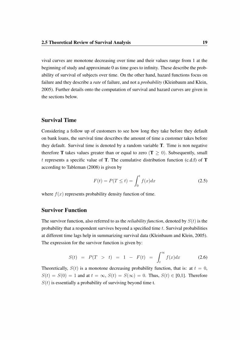
vival curves are monotone decreasing over time and their values range from 1 at thebeginning of study and approximate 0 as time goes to infinity. These describe the prob-ability of survival of subjects over time. On the other hand, hazard functions focus onfailure and they describe a rate of failure, and not a probability (Kleinbaum and Klein,2005). Further details onto the computation of survival and hazard curves are given inthe sections below.
Survival Time
Considering a follow up of customers to see how long they take before they defaulton bank loans, the survival time describes the amount of time a customer takes beforethey default. Survival time is denoted by a random variable T. Time is non negativetherefore T takes values greater than or equal to zero (T ≥ 0). Subsequently, smallt represents a specific value of T. The cumulative distribution function (c.d.f) of Taccording to Tableman (2008) is given by
F (t) = P (T ≤ t) =
∫ t
0
f(x)dx (2.5)
where f(x) represents probability density function of time.
Survivor Function
The survivor function, also referred to as the reliability function, denoted by S(t) is theprobability that a respondent survives beyond a specified time t. Survival probabilitiesat different time lags help in summarizing survival data (Kleinbaum and Klein, 2005).The expression for the survivor function is given by:
S(t) = P (T > t) = 1 − F (t) =
∫ ∞t
f(x)dx (2.6)
Theoretically, S(t) is a monotone decreasing probability function, that is: at t = 0,S(t) = S(0) = 1 and at t = ∞, S(t) = S(∞) = 0. Thus, S(t) ∈ [0,1]. ThereforeS(t) is essentially a probability of surviving beyond time t.
2.5 Theoretical Review of Survival Analysis 20
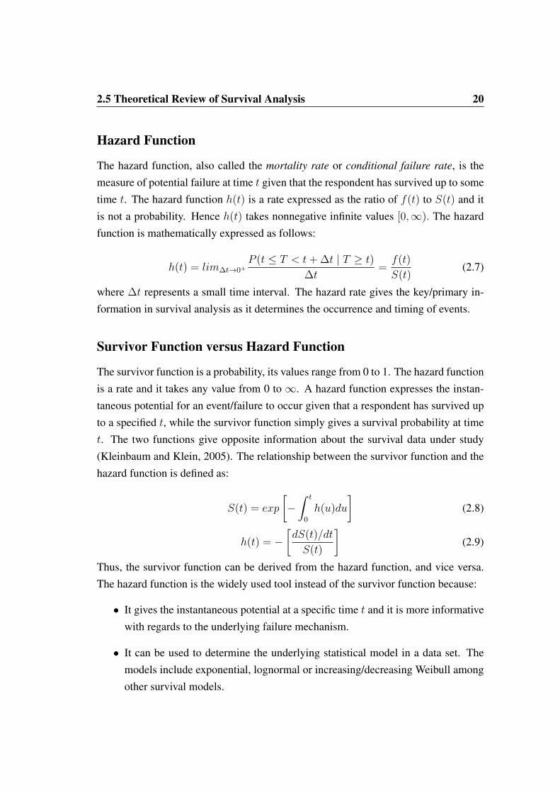
Hazard Function
The hazard function, also called the mortality rate or conditional failure rate, is themeasure of potential failure at time t given that the respondent has survived up to sometime t. The hazard function h(t) is a rate expressed as the ratio of f(t) to S(t) and itis not a probability. Hence h(t) takes nonnegative infinite values [0,∞). The hazardfunction is mathematically expressed as follows:
h(t) = lim∆t→0+P (t ≤ T < t+ ∆t | T ≥ t)
∆t=f(t)
S(t)(2.7)
where ∆t represents a small time interval. The hazard rate gives the key/primary in-formation in survival analysis as it determines the occurrence and timing of events.
Survivor Function versus Hazard Function
The survivor function is a probability, its values range from 0 to 1. The hazard functionis a rate and it takes any value from 0 to∞. A hazard function expresses the instan-taneous potential for an event/failure to occur given that a respondent has survived upto a specified t, while the survivor function simply gives a survival probability at timet. The two functions give opposite information about the survival data under study(Kleinbaum and Klein, 2005). The relationship between the survivor function and thehazard function is defined as:
S(t) = exp
[−∫ t
0
h(u)du
](2.8)
h(t) = −[dS(t)/dt
S(t)
](2.9)
Thus, the survivor function can be derived from the hazard function, and vice versa.The hazard function is the widely used tool instead of the survivor function because:
• It gives the instantaneous potential at a specific time t and it is more informativewith regards to the underlying failure mechanism.
• It can be used to determine the underlying statistical model in a data set. Themodels include exponential, lognormal or increasing/decreasing Weibull amongother survival models.

2.6 Censoring 21
• Survival models are mostly expressed in terms of the hazard function and thisbecomes handy in summarizing survival data.
The Hazard Ratio
In survival analysis, the Hazard Ratio (HR) is the measure of the effect of explanatoryvariables. The corresponding measure of the effect in a logistic regression is the oddsratio and β measures the effect of independent variables in ordinary linear regression.In survival analysis, when two samples are exposed to different treatments, say 0 and1, the HR is given by:
HR(t|1, 0) =h(t|1)
h(t|0)(2.10)
HR = 1, means there is no treatment effect. For values of HR less than 1, it impliesthe sample receiving treatment 0 has more risk of failing than the sample receivingtreatment 1, and vice versa for HR values greater than 1. The HR plays a crucial rolein survival analysis (Kleinbaum and Klein, 2005).
2.6 Censoring
In survival analysis, censoring is a term used to express incomplete data. This occurswhen we do not have the entire information about some respondents over a specifiedfollow up period. Only a part of information about the individual is known. In survivalanalysis, censoring is denoted by a dichotomous variable δ which takes values 0 or 1,to indicate whether an object was censored or not respectively. Censoring can eitherbe fixed or random.
Fixed censoring is defined in two scenarios. Type I censoring is a fixed form of cen-soring whereby subjects under investigation are subjected to the same test at the sametime and the experiment is terminated at predetermined time t. Failure times are eitherobserved or censored. In Type I censoring, t is fixed. Type II censoring involves run-ning an experiment until a predetermined number of failures, say r of the total objectsn have been achieved. The remaining observations are all censored and r is fixed.

2.6 Censoring 22
Random censoring occurs when objects enter the study at different times. Censoringoccurs when:
• A respondent relocates without traceable contacts or may fail to appear due tosome other cause. This is called loss to follow up.
• A respondent discontinues participation abruptly and drops out.
• An event hasn’t occurred when the study is terminated.
When a respondent’s information is censored using any of the above scenarios, that is,censored at the right side of observed time, we call this right censoring. Left cen-sored data occurs when the true survival time is less than or equal to the total followup period. For example, the event occurred to the respondent before the start of thestudy and the actual event time is unknown. Interval censored data is obtained whenthe event is known to have occurred between two time points but the exact time isunknown. Random censoring with right censored information is common in the con-sumer credit context.
Figure 2.1: Censoring

2.7 The Empirical Survivor Function 23
Figure 2.1 is an illustration of censorship in survival data. Four participants entered thestudy at different calender times. Subjects B and D experienced the event before thetermination of study. Subject A withdrew from the study before the event. The studywas terminated before subject C experienced an event. Both subjects A and C are rightcensored.
2.7 The Empirical Survivor Function
Survival data is composed of complete data (where an event took place) and incom-plete (censored) data. The Empirical Survival Function (ESF) calculation ignores thecensoring aspect. All observations are regarded as complete and they are ordered withrespect to the length of stay in the study, from the minimum to maximum.
Figure 2.2: Empirical Survival Curve
The ESF is denoted by Sn(t) and is calculated as follows:
Sn(t) =Number of observations at T > t
n(2.11)

2.8 The Kaplan Meier Survival Estimator 24
where n is the total number of objects under study. Plotting Sn(t) against time spentin the study gives a step function, stepping down at each time t as shown in Figure 2.2.The mean of the area under the curve is calculated as follows:
mean =
∫ ∞0
Sn(t)dt (2.12)
2.8 The Kaplan Meier Survival Estimator
The Kaplan Meier (KM) survival estimator is an extension of the ESF which gener-alises the ESF and adjusts for censored observations. The KM formula for survivalprobability at any specified time ti is limited to product terms of survival probabilitiesprior to and including the survival probability of subjects surviving beyond ti. Thus,the KM survival curve is also referred to as the product-limit estimator of survival.
For KM computation purposes, the survival data is sorted in ascending order of failuretimes. The first entry begins at survival time equals zero. At time zero, the probabilityof surviving beyond t0 is 1. Subjects yi, are eliminated at each failure point in timedue to either failure or censorship. The risk set, denoted by R(ti) is the total numberof individuals who survived up to at least a specified failure time point tj .
The KM survival estimator considers: ni = number of observations in the risk set anddi = number of subjects failing at failure time tj . The KM survival estimator is definedas:
S(tj) =
j∏i=1
P r [T > ti|T ≥ ti]
= S(tj−1)× P r [T > ti|T ≥ ti]
=
j∏i=1
(ni − dini
)(2.13)
As obtained in the ESF, the KM estimator of survival produces a step function whichsteps down only at observed failure times. The risk set at time ti excludes both failed

2.8 The Kaplan Meier Survival Estimator 25
and censored observations prior to the specified time point. Thus, the KM curve isgreater than or equal to the ESF curve. If the data set is complete and there are nocensored observations, the KM reduces to the ESF. The mean and median estimates arehigher when using the KM function compared to the ESF in the presence of censoredobservations. A KM type estimate of hazard at time point ti is given by:
h(ti) =dini
(2.14)
Comparison of Survivor Curves
Given two-sample (two treatment) survival curves, the graphs may differ judging bythe eye. An example is shown in Figure 2.3. In order to investigate if the differencebetween the two curves is statistically significant, the most commonly used tests in-clude the Log-rank Mantel-Haenszel (LMH) test and the Gehan test that adjusts forcensored data (Kleinbaum and Klein, 2005). The LMH test is the generalized log-ranktest adjusting for covariates. It gives the overall comparison of survivor curves. Thenull hypothesis states that there is no difference between the two survival curves, thatis: H0 : F1 = F2. The values of the two samples are combined and listed in ascendingorder.
Figure 2.3: Comparison of Survivor Curves
2.9 The Cox Proportional Hazards Regression Model 26
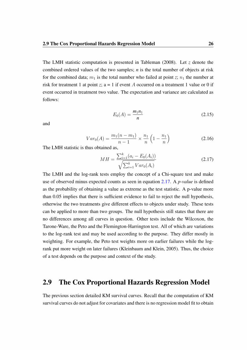
The LMH statistic computation is presented in Tableman (2008). Let z denote thecombined ordered values of the two samples; n is the total number of objects at riskfor the combined data; m1 is the total number who failed at point z; n1 the number atrisk for treatment 1 at point z; a = 1 if event A occurred on a treatment 1 value or 0 ifevent occurred in treatment two value. The expectation and variance are calculated asfollows:
E0(A) =m1n1
n(2.15)
and
V ar0(A) =m1(n−m1)
n− 1× n1
n
(1− n1
n
)(2.16)
The LMH statistic is thus obtained as,
MH =
∑ki=1(ai − E0(Ai))√∑k
i=1 V ar0(Ai)(2.17)
The LMH and the log-rank tests employ the concept of a Chi-square test and makeuse of observed minus expected counts as seen in equation 2.17. A p-value is definedas the probability of obtaining a value as extreme as the test statistic. A p-value morethan 0.05 implies that there is sufficient evidence to fail to reject the null hypothesis,otherwise the two treatments give different effects to objects under study. These testscan be applied to more than two groups. The null hypothesis still states that there areno differences among all curves in question. Other tests include the Wilcoxon, theTarone-Ware, the Peto and the Flemington-Harrington test. All of which are variationsto the log-rank test and may be used according to the purpose. They differ mostly inweighting. For example, the Peto test weights more on earlier failures while the log-rank put more weight on later failures (Kleinbaum and Klein, 2005). Thus, the choiceof a test depends on the purpose and context of the study.
2.9 The Cox Proportional Hazards Regression Model
The previous section detailed KM survival curves. Recall that the computation of KMsurvival curves do not adjust for covariates and there is no regression model fit to obtain
2.9 The Cox Proportional Hazards Regression Model 27
survival estimates. In a real life scenario, covariates are inevitable and they influencesurvival estimates. Exclusion of covariates in the calculation of survival curves mayresult in less accurate results. Cox (1972) developed a regression model which out-puts adjusted survival curves by including covariates in the computation of survivalestimates. The Cox PH regression methodology has gained popularity for it is flexibil-ity and use of a small number of assumptions to obtain the basic information requiredfrom survival analysis, namely the HR which is obtained from the Cox hazard functionand survival information obtained from the Cox model survival function.
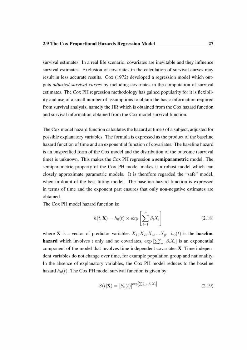
The Cox model hazard function calculates the hazard at time t of a subject, adjusted forpossible explanatory variables. The formula is expressed as the product of the baselinehazard function of time and an exponential function of covariates. The baseline hazardis an unspecified form of the Cox model and the distribution of the outcome (survivaltime) is unknown. This makes the Cox PH regression a semiparametric model. Thesemiparametric property of the Cox PH model makes it a robust model which canclosely approximate parametric models. It is therefore regarded the “safe” model,when in doubt of the best fitting model. The baseline hazard function is expressedin terms of time and the exponent part ensures that only non-negative estimates areobtained.The Cox PH model hazard function is:
h(t,X) = h0(t)× exp
[p∑i=1
βiXi
](2.18)
where X is a vector of predictor variables X1, X2, X3, ...Xp. h0(t) is the baselinehazard which involves t only and no covariates, exp [
∑pi=1 βiXi] is an exponential
component of the model that involves time independent covariates X. Time indepen-dent variables do not change over time, for example population group and nationality.In the absence of explanatory variables, the Cox PH model reduces to the baselinehazard h0(t). The Cox PH model survival function is given by:
S(t|X) = [S0(t)]exp[∑p
i=1 βiXi] (2.19)

2.9 The Cox Proportional Hazards Regression Model 28
2.9.1 Maximum Likelihood Estimation of the Cox Regression Model
Typical parametric regression models depend on some specified distribution of the re-sponse variable which forms the basis for the likelihood function. A full likelihoodfunction is derived for parametric regression models whereas Cox regression uses thepartial likelihood function. Cox regression makes no distributional assumption of thedependent variable (time to event). The regression coefficients, β′s in a Cox regres-sion model are the maximum likelihood estimates. The coefficients are derived bymaximising a likelihood function L = L(β) which is equal to the joint probability ofobserved data. Lj is a “partial” likelihood function as its computation considers proba-bilities for subjects who fail together with elements in the risk set. It does not considerthe probabilities of censored subjects. Partial likelihood is determined at each failuretime and is expressed as the product of likelihoods per each failure time. Thus, for kfailure times,
L = L1 × L2 × L3 × ...× Lk =k∏j=1
Lj (2.20)
Once the likelihood function is obtained, the next step maximises this function by max-imising the natural log of L through a series of iterations. The maximization process isdone through the mathematical differentiation process and setting the differential equalto zero.
dln(L)
dβi= 0 i = 1, 2, 3, ..., p. (2.21)
2.9.2 Tied Event Times in Cox PH Regression
The concept of partial likelihood estimation of regression parameters assumes no tiedevent times. However, tied event times are inevitable in consumer credit data and thereare various approaches to treat tied events in survival analysis. Hubber and Patetta(2013) briefly described the different approaches used to modify the partial likelihoodestimation to accommodate ties.
The exact method considers all possible orderings of the tied event times to computethe partial likelihood. It assumes that ties are due to lack of precision in measuring sur-vival time. The exact method is computer intensive with large data sets. The discrete
method assumes events occurred at exactly the same time. It replaces the proportional

2.9 The Cox Proportional Hazards Regression Model 29
hazards model with the logistic model and computes the probabilities that the eventsoccurred to a set of subjects with tied event times. It is also very computer intensivefor large data sets with many ties.
The Breslow method approximates the exact method (Hubber and Patetta, 2013). Ityields coefficients biased towards zero when the number of ties is large. It is lesscomputer intensive compared to exact and discrete methods. The Efron method yieldscoefficients that are closer to the exact method and give a close approximation to theexact method. It uses less computer time compared with the Breslow method. If thereare no ties in the data set, all methods described above result in the same likelihoodand yield identical parameter estimates. Where the data set is big and there is a largenumber of ties, the Efron method is preferred.
According to Hertz-Picciotto and Rockhill (1997), the Breslow and Efron estimatesare computed as follows: Let xl be the vector of explanatory variables for the lth indi-vidual. Let the ordered failure times be t1 < t2 < t3 < ... < tk. Let Di be the set ofindividuals who failed at time ti, di be the size of set Di and Ri be the risk set at timeti. Denote υi = exp
[(∑lεDi
xl)′β].
The likelihood for the Breslow approximation is:
L(β) =k∏i=1
{υi[∑
lεRiexp(x
′lβ)]di}. (2.22)
The likelihood for the Efron approximation is:
L(β) =k∏i=1
υi
di∏j=i
[∑lεRi
exp(x′lβ)− j−1
di
∑lεRi
exp(x′lβ)] . (2.23)
2.9.3 Computation of the Hazard Ratio
Recall that, the HR is the measure of effect in survival analysis. HR in a Cox PH modelis determined using the β′s of the exponential part of the formula. It shows us the ef-fect of explanatory variables even without estimating the baseline hazard function. We

2.9 The Cox Proportional Hazards Regression Model 30
can thus, obtain the hazard and subsequently the survival function using a minimumof assumptions (Kleinbaum and Klein, 2005). This makes the Cox model the mostappealing approach to analysing survival data. However, the Cox PH model assumes aconstant HR for any two subjects over time.
HR is defined as the hazard for one subject divided by the hazard for another subject inthe same study. The two subjects are distinguished by their values for the explanatoryvariables. Suppose two subjects’ predictor values are denoted by X
′and X respec-
tively, where
X′
= (X′1, X
′2, X
′3, ..., X
′p) and X = (X1, X2, X3, ..., Xp)
then the HR comparing the above subjects is computed in terms of regression coeffi-cients obtained using the Cox hazard function as illustrated below:
HR =h(t,X
′)
h(t,X)=h0(t)× exp
[∑pi=1 βiX
′i
]h0(t)× exp [
∑pi=1 βiXi]
(2.24)
The baseline hazard function is the same for both subjects in the same study theforeit cancels out and HR is computed using the exponential part of the Cox hazard for-mula. Using the mathematical rules of algebra on the exponent part, the HR is furtherreduced to:
HR = exp
[p∑i=1
βi(X′
i − Xi)
](2.25)
Thus, from the above computation, the HR is independent of the baseline hazard func-tion. It is also independent of time if and only if the predictor variables are not timevarying.
2.9.4 The Cox Proportional Hazards Assumption
The Cox PH assumption states that the HR for any two individuals in the same studyis constant over time. In other words, the hazard for a subject is proportional to the
2.9 The Cox Proportional Hazards Regression Model 31
hazard for another subject in the same study where the proportionality constant, say θis independent of time (Kleinbaum and Klein, 2005).
θ = exp
[p∑i=1
βi(X′
i − Xi)
](2.26)
This implies thath(t,X
′) = θh(t,X) (2.27)
The Cox PH model is appropriate for use when the PH assumption is met. When theHR vary with time, for example where hazards cross or when time varying confound-ing variables are present the PH assumption maybe violated, making it inappropriateto use the Cox PH model. Where the Cox PH assumption is not met, variations of theCox model can be used, for example the extended Cox regression or the stratifiedCox regression depending on the context.
2.9.5 Assessment of the Cox Proportional Hazards Assumption
The Cox PH model assumes a constant HR comparing any two subjects in the samestudy over time. There are various approaches used to evaluate the reasonableness ofCox PH assumption. These include, inter alia the graphical approach, goodness of fittests as well as the time dependant variables assessment.
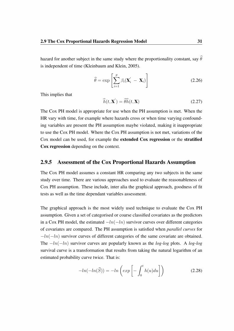
The graphical approach is the most widely used technique to evaluate the Cox PHassumption. Given a set of categorised or coarse classified covariates as the predictorsin a Cox PH model, the estimated −ln(−ln) survivor curves over different categoriesof covariates are compared. The PH assumption is satisfied when parallel curves for−ln(−ln) survivor curves of different categories of the same covariate are obtained.The −ln(−ln) survivor curves are popularly known as the log-log plots. A log-log
survival curve is a transformation that results from taking the natural logarithm of anestimated probability curve twice. That is:
−ln(−ln(S)) = −ln(exp
[−∫ t
0
h(u)du
])(2.28)

2.9 The Cox Proportional Hazards Regression Model 32
where∫ t
0h(u)du is the cumulative hazard function resulting from the formula for the
relationship between survival curves and hazard function that is given by:
S(t) = exp
[−∫ t
0
h(u)du
]The first log of a survival curve is always negative because mathematically the log ofa fraction is negative. Therefore the first log is negated and the value becomes positiveto allow for the second log. Recall from calculus that the log of a negative numberis undefined. However, after taking the log twice the final result can be positive ornegative. While the scale of the y axis of a survival curve ranges between 0 and 1 forthe survival curve being a probability, the corresponding scale for a −ln(−ln) rangebetween −∞ to +∞. This allows more flexibility and inferences regarding the PHassessment (Kleinbaum and Klein, 2005).
The algebraic formulation of the log-log curves stems from the Cox PH survival curvegiven by:
S(t|X) = [S0(t)]exp[∑p
i=1 βiXi]
Taking the first log :
ln(S(t|X)) = exp
[p∑i=1
βiXi
]× ln [S0(t)]
Taking the second log :
ln [−ln(S(t|X))] = −p∑i=1
βiXi − ln [−lnS0(t)]
−ln [−ln(S(t|X))] = +
p∑i=1
βiXi + ln [−lnS0(t)] (2.29)
Hence, after taking the log twice on the survival probability, the log − log curvecan be defined as the summation of two terms, which are the linear sum of βiXi
and the log(−log) of the baseline hazard function. The log − log curve compar-ing two subjects with different specifications of predictors X1 and X2 where X1 =
(X11, X12, X13, ..., X1p)

2.10 Model Building Process 33
and X2 = (X21, X22, X23, ..., X2p) is thus computationally reduced to an expressionthat drops out the baseline hazard function and therefore does not involve time.
−ln[−ln(S(t,X1))] = −ln[−ln(S(t,X2))] +
p∑i=1
βi(X2i −X1i) (2.30)
−ln[−ln(S(t,X2))] = −ln[−ln(S(t,X1))] +
p∑i=1
βi(X1i −X2i) (2.31)
The algebraic reduction of terms yields a linear sum of the differences in correspond-ing predictor values for the two subjects. Hence if the Cox PH model is used and thelog-log survival curves of the above two subjects are plotted on the same graph, thetwo plots would be approximately parallel. The distance between the two curves isthe linear expression involving the differences in predictor values which does not in-volve time. If the vertical distance between the curves is constant over time, then thecurves are parallel. (Kleinbaum and Klein, 2005). Cox PH model is appropriate if theempirical plots of log-log survival curves are parallel.
2.10 Model Building Process
The first step in model building is Exploratory Data Analysis (EDA). This involvesexamining the empirical Kaplan Meier survival curves, assessing the results of thelog-rank test, distribution of survival time, univariate and multivariate analysis of co-variates. EDA is crucial in identifying numerical issues and potential errors embeddedin the data set. The distribution of individual covariates is considered over time andconsistency is assessed overtime. Covariates are examined one on one with the depen-dent variable using Weight of Evidence (WoE), which is discussed in section 2.10.2.WoE is the most widely used variable transformation tool in credit scoring (Hubberand Patetta, 2013). The ability of each variable to differentiate risk is determined usingthe GS.
2.10.1 Exploratory Data Analysis
Selection of variables to include in modelling involves exploration of individual vari-ables in a process called univariate analysis. The one on one relationship between the

2.10 Model Building Process 34
dependant variable and each of the candidate covariate is analysed using WoE and GS.Binning of individual variables is performed at the univariate analysis stage. Multi-variate analysis selects the final and supposedly the “best” variables which go togetherin the final model. Stepwise regression works out partial associations and may dealwith cases of multicollinearity (Hubber and Patetta, 2013). Correlation analysis anal-yses the one on one relationship between variables and the result usually complementsstepwise regression analysis. The decision to select which variables to use is up to theresearcher.
2.10.2 Univariate Data Analysis
In a typical data set with credit information, ordinal, continuous and nominal variablesexist. For modelling purposes, often only the interval independent variables are re-quired. Therefore it might be necessary to transform and create dummy variables. Themost commonly used transformation method is called WoE. The WoE process con-verts any variable into a numeric interval variable. Groups/classes/bins are assignedaccording to the risk of the group expressed by the logarithm of likelihood ratios, thatis logarithm of a portion of, say defaulted versus non defaulted subjects (Jilek, 2008).WoE refers to the set of “goods”, customers who do not default and the “bads”, cus-tomers who default or settle accounts early.
wij = ln
(pijqij
)(2.32)
where wij is the WoE, pij is the number of good risks in level/attribute j of vari-able/characteristic i divided by the total number of good risks who responded to i andqij is the number of bad risks in attribute j of characteristic i divided by the number ofbad risks in attribute j who responded to characteristic i. The WoE curve should be amonotonic function across the categories of a covariate.
Variables can be selected using the Information Value (IV). It measures the differencebetween distributions of the good and the bad risk on a specific covariate. Character-istics with an information value of over 0.1 will be considered for model development

2.10 Model Building Process 35
(Hand and Henley, 1997). Using WoE definitions described above,
IV =∑ij
(pij − qij)× wij (2.33)
Gini (1936) was an Italian demographer, sociologist and statistician who developeda measure of statistical dispersion, known as the Gini coefficient. It determines thelevel of inequality of a distribution. A value of 0 represents total equality and a valueof 1 represent maximal inequality. The values are usually expressed as a percentage.In the area of economics, the coefficient was developed mainly to measure inequalityof income or wealth of many different nations worldwide. The Gini Coeffient gainedpopularity in other domains including engineering, sociology, chemistry, ecology andso on.
Similarly, in the field of Statistics, the GS, also known as the Somer’s D, measures avariable’s ability to differentiate risk when fitting a univariate (single input variable)logistic model. It measures uniformity of a distribution. The lower the GS, the moreuniformly distributed the variable (Jilek, 2008). In the consumer credit context, the GSstatistic is used to measure how equal the event rates are across the attributes of a vari-able. The higher the GS, the higher the ability of the characteristic to differentiate risk.All variables with a GS of less than five percent maybe excluded (Migut, Jakubowskiand Stout (2013)), however, due to the small number of covariates considered, this re-search will lower down the cut GS cut off to four percent.
In the calculation of the GS, the attributes i = 1, 2, 3, ...,m are sorted in ascendingorder of their event rates. For each of the attributes, the number of events is given byneventi , the non-event by nnon−eventi . The total number of events = N event and the totalnumber of non-events is given by Nnon−event. Then the GS is calculated as follows:
GS =
1−2×
∑mi=2
(neventi ×
∑i−1j=1 n
non−eventj
)+∑m
k=1
(neventk × nnon−eventk
)N event ×Nnon−event
×100(2.34)

2.10 Model Building Process 36
2.10.3 Multivariate Data Analysis
Variables that are not significant in univariate analysis may become significant in amultivariate model because of partial associations. Partial association refers to the ef-fect of one variable changes in the presence of other variables. Partial association ofcandidate covariates is determined using, inter alia, stepwise regression, backward orforward elimination and best subsets selection.
Best subsets selection is computer intensive when we have big data sets. Each covari-ate should have at most two categories. This study may not use best subset selectionbecause of the existence of more than two classes in some variables. Among othermethodologies, this study uses stepwise regression to identify subsets of covariates be-fitting plausible models.
Covariates are assessed for multicollinearity using the Variance Inflation Factor (VIF)as well as correlation analysis. It is imperative to assess multicollinearity amongcovariates before analysts conduct a multivariate regression analysis (Mansfield andHelms, 1982). If covariates within the model are highly correlated with each other,this would be reflected through a high VIF value. It is recommended that VIF valuesshould lie below five (Migut et al (2013)), if covariates are to be considered for modeldevelopment. However the author revised the VIF cut off to three in order to eliminateany form of multicollinearity. Any candidate covariate with a VIF of at least 3 shouldbe excluded from further analysis.
2.10.4 Goodness of Fit Measures
Type 3 tests are used to test the hypothesis that all regression coefficients in the modelare zero. Type 3 tests are Wald, Score and the Likelihood ratio tests. The Wald statis-tic also known as the Z statistic is used with the maximum likelihood estimates tocompute the p-value (the probability of obtaining a value as extreme as the test statis-tic). The p-value helps the researcher to decide whether to fail to reject or reject theunderlying hypothesis about the variables being assessed usually if the p-value is lessthan α = 0.001. The Score test is similar to the Wald test. The Likelihood Ratiois an alternative statistic, which makes use of the log likelihood statistic, −2 × lnL.

2.10 Model Building Process 37
The p-values for Wald static and Likelihood Ratio may not yield the same p-value butgenerally the conclusion is the same unless there is multicollinearity present. From ex-pert opinion, Kleinbaum and Klein (2005) suggest that when in doubt, the researchershould use Likelihood Ratio test.
The Likelihood Ratio is also used to compare model fit. For example, the LikelihoodRatio comparing model one and model two is computed as follows: Likelihood Ra-tio = -2ln(Lmodel1) - (-2ln(Lmodel2)). Likelihood Ratio follows a χ2 distribution andthe corresponding p-value is obtained, leading to conclusions on the hypothesis H0:Model 1 = Model 2 and H1: Models differ. P-values less than α = 0.001 suggest thattwo models are significantly different. The Akaike Information Criterion (AIC) andthe Schwarz Bayesian Criterion (SBC), also known as Bayesian Information Criteriaare also goodness of fit measures used to compare one model to another. The differ-ence between AIC and SBC lie in the penalties used for extra variables. SBC penalty ismore severe and therefore uses more parsimonious models (Hubber and Patetta, 2013).The lower the goodness of fit measures the better the model.
Other model diagnostics measures include the assessment of residuals. In survivalanalysis, the mostly commonly used residuals are the Cox-Snell (Cox and Snell, 1968)residuals and the Schoenfeld residuals (Schoenfeld, 1982).
Cox-Snell residuals are computed as follows:
rci = exp(βxi)H0(ti) = Hi(ti) = −log(Si(ti)) (2.35)
where H0(ti) is the cumulative baseline hazard and Hi(ti) is the estimated cumulativehazard for the ith individual at time ti and Si(ti) is the estimated survivor functionof the ith individual at time ti. Si(ti) has an exponential distribution with unit mean(Stepanova and Thomas, 2002). If the model is adequate, a plot of log(−log(Si(ti)))
against rci should give a straight line with a unit slope and zero intercept. Schoenfeldresiduals are interpreted in a similar way except that their output includes residuals andvalues for every covariate conditional on the risk set.

2.11 Competing Risks Survival Analysis 38
2.10.5 Assessment of Model Performance
Model assessment is based on the validation set. The basic methods of assessment in-clude separability measures and the counting methods. Separability measures such asthe divergence statistic (the value of the sample t-statistic between the two design setclasses) are not reviewed in this study. Rather, counting measures are used for modelperformance assessment.
Counting measures are based on a two by two contingency table of predicted by actualclasses. A Lorentz curve shows the cumulative proportion of true goods plotted againstthe proportion of true bads as the threshold varies. A similar computation is done forthe Receiver Operating Characteristic (ROC) curve wherein the true positive rate isplotted against the false positive rate (Hand and Henley, 1997). The area between thecurve and the axes is used as the discriminatory power of the model. A transformation,called GS is a measure of twice the area between the curve and the diagonal (idealclassifier). A better fitting model scores the higher value.
2.11 Competing Risks Survival Analysis
Standard survival analysis methodology considers a single event in a study. Survivalcurves in such cases can be computed using the Kaplan Meier approach if no covariateadjustment is desired. However, when two or more events are determined in a sin-gle study, the statistical problem is defined as a competing risk problem as each event“competes” to be the cause of failure.
The KM approach may not be used in the presence of competing risks as it becomesvery sensitive and may produce biased results. The modeling methodologies ideal forcompeting risks include the Cox PH model, parametric survival models and the CIC.The Cox PH regression cause specific methodology is widely used to model competingrisks. Where each event type is modeled separately and other event types are treatedas censored categories, the approach is called the “cause specific” method.

2.11 Competing Risks Survival Analysis 39
2.11.1 The Cause Specific Approach
The most widely used approach to competing risks is the cause specific approach.Stepanova and Thomas (2002) illustrated the “cause-specific” methodology to com-peting risks. The analysis was based on the U.K consumer credit data, obtained froma major U.K financial institution.
Consider default as event type 1 and ES as event type two. The cause specific approachfits two separate Cox regression models, one for each failure type. Stepanova andThomas (2002) estimated the time until default T1 and assumed the rest of observedlifetimes to be censored, including the subjects who entered into the early repaymentbucket. A second model analogous to the first one was fit and estimated time untilrepayment T2, assuming other observed lifetimes to be censored, including the subjectswho defaulted. A Cox PH model was fit in each case, on T1 and T2. From literature,the predicted lifetime of a loan is thus T = min(T1,T2, term of the loan). In thisanalysis, the cause specific hazard functions of the two events are:
h1(t) = lim∆t→0P (t ≤ T1 < t+ ∆t|T1 ≥ t)/∆t (2.36)
h2(t) = lim∆t→0P (t ≤ T2 < t+ ∆t|T2 ≥ t)/∆t (2.37)
where the random variable T1 = time to failure from default, and T2 = time to failuredue to early repayment. h1(t) and h2(t) give the instantaneous failure rates at t fordefault and early repayment respectively.
In general, given c events in an analysis, the Cox PH cause specific model is given by:
hc(t,X) = h0c(t) exp
[p∑i=1
βicXi
](2.38)
In this analysis, when c = 1 a default event is modelled and the rest of the observed life-times are treated as censored. If c = 2, a model for early repayment is obtained, holdingother observations as censored. X = (X1, X2, X3, ..., Xp) is a vector of explanatoryvariables included in the study. The βic’s are event specific regressions parameters.

2.11 Competing Risks Survival Analysis 40
2.11.2 The Cumulative Incidence Curve
The CIC is an alternative summary curve to the KM survival curve. CIC estimates the“marginal probability” of an event. CIC has more meaningful interpretation in termsof treatment utility inspite of whether competing risks are independent or not. Themarginal probability for each event type c at failure time ti is computed as follows:
CICc(ti) =i∑i=1
S(ti−1)hc(ti) (2.39)
where
S(ti−1) is the overall survival probability of surviving previous time ti−1. This com-putes subjects surviving all competing risks. The hazard estimate hc(ti) for event typec is the proportion of subjects failing from event c at time ti.
hc(ti) =mci
ni(2.40)
where mci is the number of subjects failing from event type c and ni is the risk set.
When computing CIC of a single event type, the CIC reduces to a (1− (KM)) curve.CIC does not rely on the independence assumption of competing risks unless the“cause specific” hazards model is used as an intermediate step to obtain HR estimatesfor individual competing risks. Fine and Gray (1999) modelled the CIC and regresseddirectly on the CIC and not on the cause specific hazards and their methodology isregarded as an improvement on cause specific hazards as it corrects the mismatch ef-fect of covariates on cause specific hazards and CIC when hazard functions are usedas an intermediate step. The resultant curve was referred to as the subdistribution, themarginal probability function, the crude incidence and sometimes the absolute causespecific risk.
Thus, the CIC is a generalisation of the (1-(KM)) curve. It accommodates multipleevent types in its computation. In the absence of competing risks, it reduces to (1-
2.12 Parametric Models of Survival 41
(KM)). In this analysis, the CIC curve for default is given by:
CIC(ti) =i∑i=1
S(ti−1)h1(ti) (2.41)
where
S(ti−1) is the overall survival probability of surviving up to a previous time ti−1. Thiscomputes subjects surviving both default and ES. The hazard estimate h1(ti) for defaultevent is the proportion of subjects failing from event default at time ti.
h1(ti) =m1i
ni(2.42)
wherem1i is the number of subjects failing from default event and ni is the risk set.
A separate CIC curve of ES (event type = 2) is fit with steps analogous to the defaultevent one described above. Fine and Gray (1999) used adjusted hazard estimates ofeach event type as input into the CIC curves and noted that the effect of a covariateon the cause specific hazard of a particular failure type maybe very different fromthe effect of the covariate on the corresponding CIC. Moreover, when cause specificformulation is used as the intermediate step in CIC construction, testing for covariateeffects on the subdistribution CIC is not possible. To this effect, the authors intro-duced a proportional hazard model for the subdistribution grounded in the log(-log)transformation of the univariate survival data.
2.12 Parametric Models of Survival
Parametric survival models are based on specified distribution of the outcome (survivaltime) expressed in terms of unknown parameters. Most commonly used distributions inparametric survival models include exponential, Weibull, log-logistic, lognormal andgeneralised gamma. Parametric models are mainly Accelerated Failure Time (AFT)models whereby the outcome is expressed in terms of explanatory variables. The AFTmodel shows the effect of explanatory variables on survival time. AFT models are
2.12 Parametric Models of Survival 42
designed to accommodate left, right and interval censored data while the PH modelscan only handle right censored data (Hubber and Patetta, 2013). AFT model assumesthe effect of covariates is proportional over time. Recall that the PH model assumes aconstant HR over time and it gives the effect of predictor variables on the hazard. Thus,AFT models compare survival times while the PH models compare hazards using thenumeric acceleration factor and the HR respectively.
In mathematical transformation theory, the acceleration factor in an AFT model isreflected as the “stretch” factor between two survivor functions. It either stretches orcontracts survival functions being compared. If sample one receives treatment one andsample two receives treatment two, S2(t) can be expressed in terms of S1(t) using aconstant λ which is the acceleration factor in an AFT model. That is S2(t) = λS1(t).An acceleration factor greater than one implies treatment two promotes survival λtimes, the reverse is true for λ less than one.
2.12.1 The Weibull Distribution
The survival S(t) and hazard h(t) functions of Weibull distribution are:
S(t) = e−λtp
and h(t) = λptp−1
p is the shape parameter and it governs the the shape of the hazard function for exam-ple the “bathtub” and the “cup” shapes. A special and unique property of the Weibullmodel is, “if the AFT assumption holds then the PH assumption also holds”, (Klein-baum and Klein, 2005). It holds for a fixed shape parameter p.
2.12.2 The Exponential Distribution
The survival S(t) and hazard h(t) functions of exponential distribution are:
S(t) = e−λt and h(t) = λ
The exponential distribution is regarded as the simplest because its hazard rate is con-stant over time. It is a special case of a weibull model where p = 1 (see Weibull) thehazard function becomes a constant. Exponential model can allow for both the PH

2.13 Mixture Models of Survival 43
and AFT assumptions. The constant hazard function λ can be reparameterized andexpressed as a PH model.
2.12.3 The Log-logistic Distribution
The survival S(t) and hazard h(t) functions of the Log-logistic distribution are:
S(t) =1
1 + λtpand h(t) =
λptp−1
1 + λtp
2.13 Mixture Models of Survival
Before the use of survival regression models, it is imperative to explore the non-parametric KM survival and hazard curves. Survival methods discussed in the pre-vious section assume the empirical survival curve levels off at zero as time goes to+∞. If the survival curve levels off to non zero proportions, then the standard survivalmethodologies may be inappropriate.
Empirical survival curves may level off to non zero proportions in cases where somesubjects in study are not susceptible to the event(s) of interest. That is, given an ex-tended observation period, the bulk of accounts may never default nor pay-off early.These are called long-term survivors. As most customers are “good” customers, weare likely to have long-term survivors in this study. Approaches to modelling lifetimedata in the presence of long-term survivors are called cure models or mixture models.
Literature on mixture models is found in the works of Farewell (1982) as well as Syand Taylor (2000). Mixture or cure models are designed to cater for a sizeable propor-tion of subjects who do not experience the event of interest at the end of the observationperiod. “A KM survival curve that shows a long and stable plateau with heavy censor-ing at the tail maybe taken as empirical evidence of a cured fraction”, Sy and Taylor(2000, page 228).

2.14 Conclusion 44
2.13.1 The Proportional Hazards Mixture Model
A mixture of two populations is considered, the susceptible, will be denoted populationA and the non-susceptible (long-term survivors) population B. A binary indicator isadded to distinguish between subjects falling in the two populations. Let Y = 1 if theaccount defaults/ pay-off early eventually and Y = 0 otherwise. Define p = Pr(Y =1),T = time to an event of subjects only in population A. The proportion of B = 1-p. Thesurvivor function of the entire population (A + B) is given by:
S(t) = (1− p) + pSA(t) (2.43)
where SA(t) is the survivor function of population A.
2.14 Conclusion
In this section, methods of modeling credit risk were discussed, from the pre computerera to present day methodologies. Judgemental methods were based on expert opin-ion of experienced officers. Credit granting decisions were gender and marital statussensitive, before the ECOA was introduced. The current methodologies are guidedby legislature and all individuals are granted equal opportunities. Statistical modelsof credit highlights the possible statistical methods of credit scoring including multi-ple linear regression, logistic regression and survival analysis. The progression of onemethod used to another was detailed in this section indicating the strength and weak-nesses of techniques when employed in credit modelling. Survival analysis methodsare believed to be superior to most statistical methods in building credit risk models.
The usage of parametric survival methods require an accurate specification of themodel before usage. This is oftenly difficult to determine, hence the use of a semi-parametric survival method, the Cox PH regression methodology. The Cox PH re-gression technique is known to be a robust method which can closely approximateparametric regression estimates. In the presence of competing risks, the Cox PH re-gression method is employed for each cause of failure in a cause-specific regression.Cause specific models are used as intermediate step into the calculation of CIC whichestimates the marginal probabilities of each event in the presence of the other events.

2.14 Conclusion 45
The CIC is ideal in credit risk for the calculation of PD, LGD and EAD models. In thepresence of long term survivors, mixture models of survival are the most appropriate.
Chapter 3
Methodology
3.1 Introduction
The scope of this study is statistical analysis of loans extended for the purpose of ve-hicle purchases in a retail framework. The purpose is to analyse competing risks ina consumer credit context. Data set is obtained from a major South African financialinstitution. As in a normal statistical analysis scenario, EDA is necessary for us toengage and familiarise ourselves with the data, to detect any possible anomalies, to ob-tain the trends and structure of the data. EDA involves univariate and multivariate dataanalysis as well as trend analysis over time. Models are built to compare performanceof methods currently applied by financial institutions for behavioural scoring. Logisticregression and Cox regression methods are compared to determine the superior tech-nique in the presence of competing risks, default and early repayment. A detailedanalysis focuses on the possibilities and pitfalls in different modelling approaches.
3.2 Data
Vehicle finance data is obtained from a leading South African financial institution. Allthe information required is extracted from the institution data warehouse, for the period01 April 2009 to 31 March 2014. The information includes details from the applicantsand details from vehicle manufacturers. The raw data set comprise all active accounts.Accounts entering the study after the observation start date, 01 April 2009 are treated

3.2 Data 47
as left truncated entries. Granular detail is given per month per account.
The data set comprise the standard, application and behavioural variables. Standardvariables are customer key identifiers. These include the customer account number, IDand address, inter alia similar identifiers. Some standard variables shall be masked inthis study for the purposes of commercial confidentiality.
Application variables are further divided into customer specific and vehicle specificvariables. Behavioural variables are mainly customer specific, detailing repaymentbehaviour after obtaining the vehicle finance. For the purposes of this study more vari-ables are derived for example age of asset, survival time and account status indicator.Some of the derived fields shall be added as independent or standard variables usedto enhance model development and ease of computation respectively. The standardvariables are given in Table 3.1.
Table 3.1: Standard VariablesVariable Name Description/Usage
Account Number Masked customer key and unique identifier
Month Cohort indentifier
Product Code Instalment Sale product Identifier
Balancing Segment Retail Accounts Identifier
Start Month Start to follow up date
Default Month Event month
ES Month Event month
Account Balance Calculates exposure
Accumulated Interest Amount Calculates exposure
Survival Time Number of months between the entry and exit points
Table 3.2 is a list of customer and vehicle specific application and behavioural variableswhich make up part of possible candidate covariates. Additional covariates will bederived.

3.2 Data 48
Table 3.2: Customer and Vehicle Specific Covariates
Variable Short Name Variable Name Description
Vage Age of Vehicle Age of vehicle in years
Amt Fin Amount financed Loan amount extended
ATC Article Type Code Vehicle Type
DTC Dwelling Type Code Describes the residential environment
Inst Freq Instalment Frequency Frequency of instalments
Maint Code Maintenance Code Indicates maintenance of the vehicle
Manf Code Manufacturer Code Vehicle brand
Marital Status Marital Status Code Applicant’s Marital status
M&M Code M&M Code TransUnion’s Mead and McGrouther
Code
New Old Used New/Old/Used Vehicle Status
Num Dep Number of Dependants Total number of dependants
Num Ins Number of Insurances Count of Insurances held by applicant
Orig Term Original Term Original Term
SA Cit SA Citizen Ind SA Citizen or not
Spse Emp Ind Spouse Employed Indicator Indicates if spouse is employed or not
Time Curr Add Time at current address Time at current address in years
Time Curr Job Time in current Job Time at current job in years
Yr Mod Year Model Year model of vehicle
LTV Loan to Value Outstanding balance as a percentage of
current value of vehicle
Pay Mthd Cd Payment Method Code Indicates payment method
Out Term Outstanding Term Remaining Term
PrevD Number of Previous Defaults Count of previous defaults for each ac-
count

3.3 Exploratory Data Analysis 49
3.3 Exploratory Data Analysis
Data extraction and addition of derived fields is processed in SAS R©. Additional fieldsinclude, inter alia, retail indicator, survival time, status variable and other input vari-ables deemed necessary. Survival data structure is assessed through a SAS R© proce-dure, proc lifetest, to determine the shapes of hazard and survivor curves and to makeinferences around the underlying model. The full data set is randomly split into 80percent development set and 20 percent validation set. The split is consistent with theinstitution’s internal model building standards. Model development uses the develop-ment set and models are evaluated based on the validation set.
The development set is imported into SAS R© Enterprise Miner. Credit scoring optionis selected and the interactive binning node is used for WoE calculation, binning ofvariables and calculation of the GS for every candidate variable. Variables passing theunivariate analysis are assessed using stepwise regression and correlation analysis inEnterprise Guide. After selection and deletion, the final set of variables selected arethen used for model development.
3.4 Model Building
Let D be the generalised cause of failure, Event 1 = Default, and Event 2 = ES. If anaccount neither defaults nor settles early, then the account is right censored (c) dueto termination of study. There is no possibility of withdrawals and loss to follow upcensoring in the current data as all the accounts are kept in check to final classification.In competing risks analysis, the random variable T = survival time is thus determinedas T = min(T1, T2, Tc). The time period of interest is the time to the first event thatoccurred to each account.
3.4.1 Cox Regression Models
The fundamental cause-specific hazard function say the hazard of failing from defaultin the presence of ES is a joint distribution of T and D is given by:

3.4 Model Building 50
hdefault(t) = lim∆t→0+P (t ≤ T < t+ ∆t,D = default | T ≥ t)
∆t(3.1)
Final variables are tested for proportional hazards assumption using the graphical log-log plots. The Cox proportional hazards regression is performed on the cause specifichazards, given covariates described in the table of covariates and h0,1(t) and h0,2(t)
being the baseline cause specific hazards of default and ES respectively. Note that thebaseline population is generated using a combination of bins/classes of covariates withthe highest population in each model. Recall that the bins are created at the univariatestage.
The cause specific Cox PH regression model for default is given by:
h1(t|X,Y) = h0,1(t)× exp(β1V age+ β2Amt Fin+ β3ATC + ...+ β45PrevD+ β46Arr)
(3.2)
The cause specific Cox PH regression model for ES is given by:
h2(t|X,Y) = h0,2(t)× exp(β1V age+ β2Amt Fin+ β3ATC + ...+ β45PrevD+ β46Arr)
(3.3)
Recall that the cause specific hazard functions together with the overall survival curveare used as inputs into the calculation of the CIC for each event. The overall survivalcurve is the probability of not having failed from any cause at time ti. Thus the uncon-ditional probability of failing from default in the presence of competing risks at timeti is estimated as:
CIC1(ti) =i∑i=1
S(ti−1)h1(ti) (3.4)
where S(ti−1) is the overall survival probability of surviving previous time ti−1. Thecause specific hazard estimate h1(ti) for the default event is the proportion of subjectsfailing from event default at time ti with reference equation 3.2.
The unconditional probability of failing from ES in the presence of default event attime ti is estimated as:
CIC2(ti) =i∑i=1
S(ti−1)h2(ti) (3.5)

3.4 Model Building 51
3.4.2 Logistic Regression Models
Logistic Regression models are perfomed per event over the workout period (48 monthsperiod). The probability of failing from default event is estimated as follows:
p(D = 1|X,Y) =eα+(β1V age+β2Amt Fin+β3ATC+...+β44AIP+β45PrevD+β46Arr)
1 + eα+(β1V age+β2Amt Fin+β3ATC+...+β44AIP+β45PrevD+β46Arr)(3.6)
The probability of failing from ES event is estimated as follows:
p(D = 2|X,Y) =eα+(β1V age+β2Amt Fin+β3ATC+...+β44AIP+β45PrevD+β46Arr)
1 + eα+(β1V age+β2Amt Fin+β3ATC+...+β44AIP+β45PrevD+β46Arr)(3.7)
3.4.3 Model Assessment
Logistic regression and Cox regression methods are compared to determine the supe-rior technique in the presence of competing risks, default and early repayment. We willcompare Cox regression and logistic regression in estimating which loans are likely todefault/pay off early within a fixed outcome period. The ROC curves are used to com-pare model performance. However the area under each ROC curve can be used tosummarise model performance. This is equivalent to the overall model GS. Thus wewill compare the models ability to differentiate risk using model GS. Plots of actualversus expected events will be used to asses the ability of the models to rank order riskgroups. For LR models, the Hosmer-Lemeshow test will be used to assess goodness offit of the models under the hypothesis:
H0 : No model misfit
H1 : Model misfit

Chapter 4
Model Development
4.1 Introduction
This chapter takes the reader through the step by step model building process used inthis study. There exists a complex data structure containing a wealth of informationcovering every calender month over a five year period of observation. Model devel-opment and analysis will be implemented in the SAS R© environment. In financialinstitutions, individual accounts are observed and tracked every month from the pointof entry (open date) to the point of exit into either default or ES or to the termina-tion of study at the end of March 2014. This information illustrates a longitudinalstudy where individual customers from the same cohort go though different kinds ofbehaviours leading to default or ES or censorship at different time periods.
Survival analysis methodologies are well designed to model time to an event. In thepresence of competing risks and long term survivors, we will also investigate how Lo-gistic regression methods compare. It is interesting however, to first look at the com-position of the vehicle finance book in terms of brands on the market. We investigatewhether the composition complements the information obtained from an independentsurvey whose results are summarised in a biplot in Figure 1.1 of Chapter 1. Recall thatthe survey was conducted on a sample of popular brands of the South African automo-bile market. Do the “popular” brands in Section 1.2 command higher volumes in thevehicle finance portfolio under investigation?
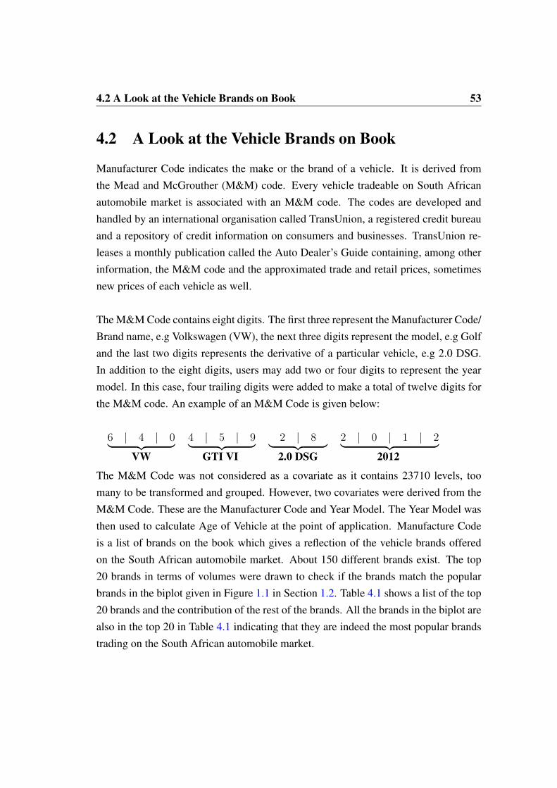
4.2 A Look at the Vehicle Brands on Book 53
4.2 A Look at the Vehicle Brands on Book
Manufacturer Code indicates the make or the brand of a vehicle. It is derived fromthe Mead and McGrouther (M&M) code. Every vehicle tradeable on South Africanautomobile market is associated with an M&M code. The codes are developed andhandled by an international organisation called TransUnion, a registered credit bureauand a repository of credit information on consumers and businesses. TransUnion re-leases a monthly publication called the Auto Dealer’s Guide containing, among otherinformation, the M&M code and the approximated trade and retail prices, sometimesnew prices of each vehicle as well.
The M&M Code contains eight digits. The first three represent the Manufacturer Code/Brand name, e.g Volkswagen (VW), the next three digits represent the model, e.g Golfand the last two digits represents the derivative of a particular vehicle, e.g 2.0 DSG.In addition to the eight digits, users may add two or four digits to represent the yearmodel. In this case, four trailing digits were added to make a total of twelve digits forthe M&M code. An example of an M&M Code is given below:
6 | 4 | 0︸ ︷︷ ︸VW
4 | 5 | 9︸ ︷︷ ︸GTI VI
2 | 8︸ ︷︷ ︸2.0 DSG
2 | 0 | 1 | 2︸ ︷︷ ︸2012
The M&M Code was not considered as a covariate as it contains 23710 levels, toomany to be transformed and grouped. However, two covariates were derived from theM&M Code. These are the Manufacturer Code and Year Model. The Year Model wasthen used to calculate Age of Vehicle at the point of application. Manufacture Codeis a list of brands on the book which gives a reflection of the vehicle brands offeredon the South African automobile market. About 150 different brands exist. The top20 brands in terms of volumes were drawn to check if the brands match the popularbrands in the biplot given in Figure 1.1 in Section 1.2. Table 4.1 shows a list of the top20 brands and the contribution of the rest of the brands. All the brands in the biplot arealso in the top 20 in Table 4.1 indicating that they are indeed the most popular brandstrading on the South African automobile market.

4.2 A Look at the Vehicle Brands on Book 54
Table 4.1: Brands on BookMANUFACTURER CODE BRAND VOLUME FREQUENCY(%)
600 TOYOTA 48899 16.64
640 VOLKSWAGEN 42802 14.57
470 NISSAN 21634 7.36
100 CHEVROLET 17038 5.80
265 HYUNDAI 16989 5.78
050 BMW 16661 5.67
440 MBENZ 16068 5.47
040 AUDI 11028 3.75
220 FORD 10868 3.70
480 OPEL 9733 3.31
280 ISUZU 8462 2.88
321 KIA 7872 2.68
540 RENAULT 6578 2.24
250 HONDA 5072 1.73
450 COLT 4832 1.64
300 JEEP 4350 1.48
350 LAND ROVER 4279 1.46
430 MAZDA 4240 1.44
598 TATA 3104 1.06
590 SUZUKI 2772 0.94
The Rest Other 30526 10.39
Total All 293807 100

4.3 Model Building Process Flow 55
A graphical view is given in the pie chart in Figure 4.1. The top five brands accountfor roughly 50% of the financial institution’s portfolio. These are Toyota, Volkswagen,Nissan, Chevrolet and Hyundai. Other popular brands occupy about 40% while theunpopular brands account for just about 10% of the portfolio. The unpopular brandscategory include the luxury, niche and other small brands. Brands associated withluxurious vehicles include Lamborghini, Maserati, Maybach, Rolls Royce and Ferrariamong others. Niche refers to a specific, specialised population of the market, exampleagricultural and trucking businesses are specialised areas. Niche brands in this caseinclude Massey Ferguson, John Deere, Leyland, DAF, Ducati and Kawasaki.
Figure 4.1: Brands on Book
4.3 Model Building Process Flow
Table 4.2 shows the steps taken in the model building process and the location of theSAS R© code at each step. Data extraction and preparation processes were covered in
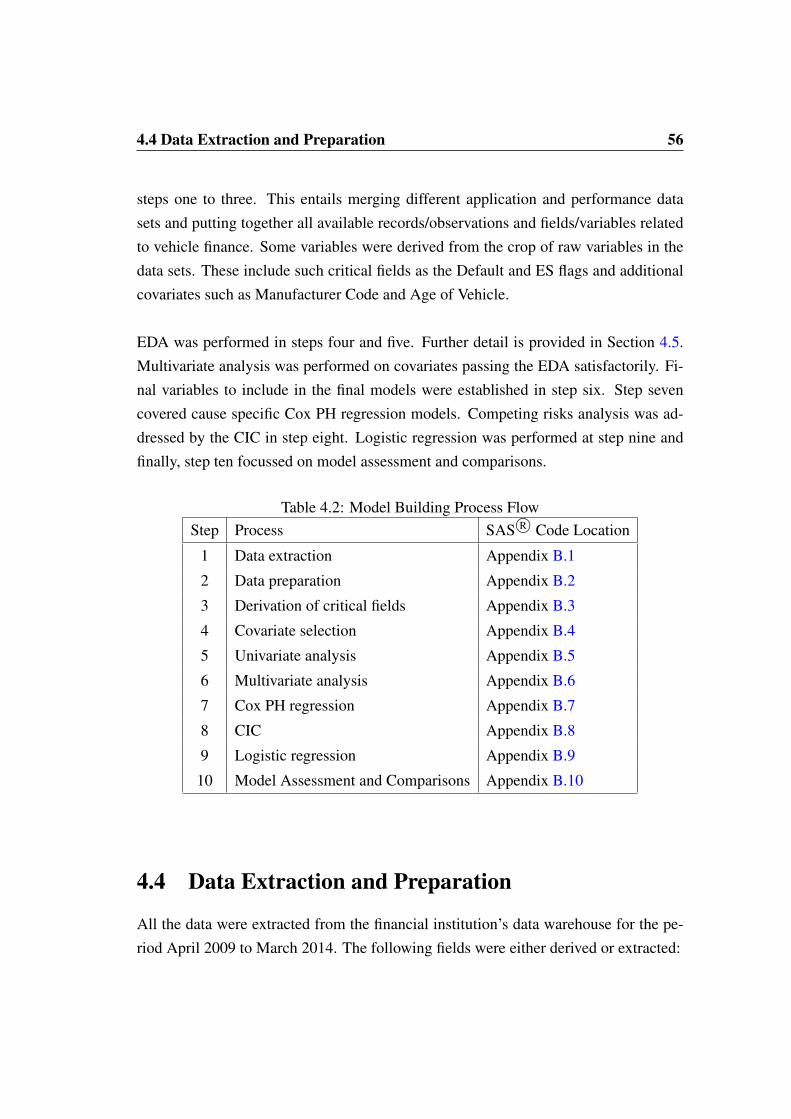
4.4 Data Extraction and Preparation 56
steps one to three. This entails merging different application and performance datasets and putting together all available records/observations and fields/variables relatedto vehicle finance. Some variables were derived from the crop of raw variables in thedata sets. These include such critical fields as the Default and ES flags and additionalcovariates such as Manufacturer Code and Age of Vehicle.
EDA was performed in steps four and five. Further detail is provided in Section 4.5.Multivariate analysis was performed on covariates passing the EDA satisfactorily. Fi-nal variables to include in the final models were established in step six. Step sevencovered cause specific Cox PH regression models. Competing risks analysis was ad-dressed by the CIC in step eight. Logistic regression was performed at step nine andfinally, step ten focussed on model assessment and comparisons.
Table 4.2: Model Building Process FlowStep Process SAS R© Code Location
1 Data extraction Appendix B.1
2 Data preparation Appendix B.2
3 Derivation of critical fields Appendix B.3
4 Covariate selection Appendix B.4
5 Univariate analysis Appendix B.5
6 Multivariate analysis Appendix B.6
7 Cox PH regression Appendix B.7
8 CIC Appendix B.8
9 Logistic regression Appendix B.9
10 Model Assessment and Comparisons Appendix B.10
4.4 Data Extraction and Preparation
All the data were extracted from the financial institution’s data warehouse for the pe-riod April 2009 to March 2014. The following fields were either derived or extracted:

4.4 Data Extraction and Preparation 57
• Entry and exit point. The entry point defines the month when the account enteredthe study starting from April 2009 onwards, while the exit point depicts the eventor censorship month. For each account, these points were determined.
• Survival time. Total number of months between entry and exit points for eachaccount.
• Account status. Status of the account at its point of exit, whether a loan is indefault or ES at the end of study.
• Censorship flag. Accounts not absorbed into default or ES were right censored atthe end of March 2014 due to termination of study and flagged with a censorshipindicator (whether the loan was censored or experienced an event).
4.4.1 Definition of Events
An account is deemed to have exited the observation period on the first occurrence ofany of the following events:
• Default event: Any account where the default definition is met is deemed de-faulted.
• Early Settlement event: Any account triggering early settlement definition wasidentified accordingly.
4.4.2 Outcome Period Analysis
The outcome period, also known as the workout period was determined on a cohortbasis. Using the full historical book, cohorts were tracked from the point of entryto absorption into different events. The outcome period depicts the amount of timeit takes for the accounts to be absorbed into default or ES. Figure 4.2 shows the cu-mulative frequencies of each event in the study period. The majority of accounts wereabsorbed within the first 48 months from the entry point. Three percent of the accountssusceptible to the events of interest exceeded 48 months in study. It was therefore de-cided to use 48 months as the outcome period. The outcome period will be used as the
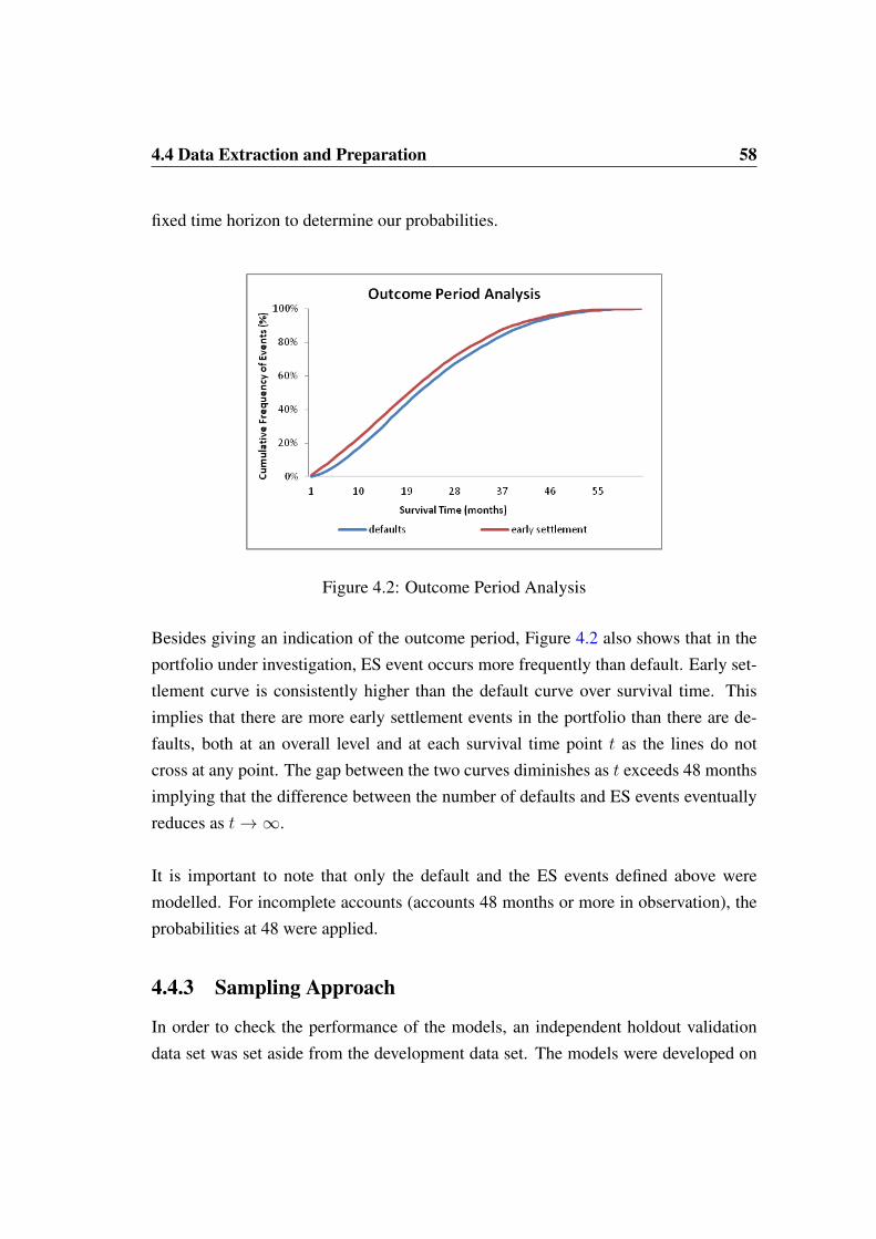
4.4 Data Extraction and Preparation 58
fixed time horizon to determine our probabilities.
Figure 4.2: Outcome Period Analysis
Besides giving an indication of the outcome period, Figure 4.2 also shows that in theportfolio under investigation, ES event occurs more frequently than default. Early set-tlement curve is consistently higher than the default curve over survival time. Thisimplies that there are more early settlement events in the portfolio than there are de-faults, both at an overall level and at each survival time point t as the lines do notcross at any point. The gap between the two curves diminishes as t exceeds 48 monthsimplying that the difference between the number of defaults and ES events eventuallyreduces as t→∞.
It is important to note that only the default and the ES events defined above weremodelled. For incomplete accounts (accounts 48 months or more in observation), theprobabilities at 48 were applied.
4.4.3 Sampling Approach
In order to check the performance of the models, an independent holdout validationdata set was set aside from the development data set. The models were developed on
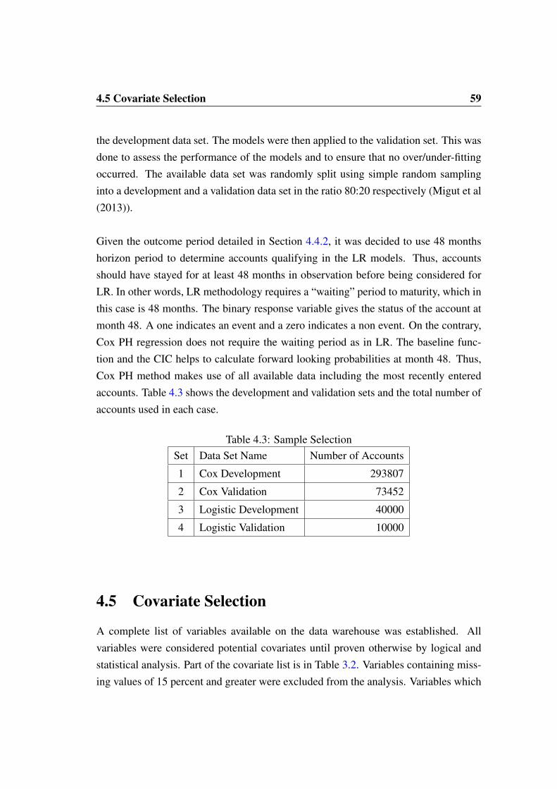
4.5 Covariate Selection 59
the development data set. The models were then applied to the validation set. This wasdone to assess the performance of the models and to ensure that no over/under-fittingoccurred. The available data set was randomly split using simple random samplinginto a development and a validation data set in the ratio 80:20 respectively (Migut et al(2013)).
Given the outcome period detailed in Section 4.4.2, it was decided to use 48 monthshorizon period to determine accounts qualifying in the LR models. Thus, accountsshould have stayed for at least 48 months in observation before being considered forLR. In other words, LR methodology requires a “waiting” period to maturity, which inthis case is 48 months. The binary response variable gives the status of the account atmonth 48. A one indicates an event and a zero indicates a non event. On the contrary,Cox PH regression does not require the waiting period as in LR. The baseline func-tion and the CIC helps to calculate forward looking probabilities at month 48. Thus,Cox PH method makes use of all available data including the most recently enteredaccounts. Table 4.3 shows the development and validation sets and the total number ofaccounts used in each case.
Table 4.3: Sample SelectionSet Data Set Name Number of Accounts
1 Cox Development 293807
2 Cox Validation 73452
3 Logistic Development 40000
4 Logistic Validation 10000
4.5 Covariate Selection
A complete list of variables available on the data warehouse was established. Allvariables were considered potential covariates until proven otherwise by logical andstatistical analysis. Part of the covariate list is in Table 3.2. Variables containing miss-ing values of 15 percent and greater were excluded from the analysis. Variables which

4.5 Covariate Selection 60
were not populated consistently back in time were excluded as well. Variables popu-lated with the same value throughout all the records were dropped. Categorical vari-ables with number of levels exceeding 150 were excluded.
Logical assessment on covariates was performed separately for numerical and categor-ical variables. The summary statistics are provided in Tables 4.4 and 4.5 respectively.To illustrate this process, a small number of covariates were selected in each case. Fornumerical data, variables with minimum value = maximum vale and a zero standarddeviation were excluded as this implies that the variable was populated with the samevalue throughout the records. Such variables do not qualify to be used as covariates.
Table 4.4: Selection of Numerical CovariatesNUMERICAL VARIABLE MIN MAX STANDARD
DEVIATION
DECISION
MADE
DEBIT INTEREST RATE 0 29.50 2.71 KEEP
NUMBER OF DEPENDANTS 0 9 0.48 KEEP
NUMBER OF ENQUIRIES 0 0 0 DROP
NUMBER OF INSURANCES 0 4 0.81 KEEP
SPOUSE INCOME AMT 0 1401195 5968.29 KEEP
TIME AT CURRENT ADD 0 0 0 DROP
TIME IN CURRENT JOB 0 99 8.71 KEEP
A similar logical analysis was performed on categorical variables. Covariates with onelevel were excluded. As discussed in the first paragraph of Section 4.5, categoricalvariables with more than 150 levels were excluded, a special exception was made forManufacturer Code and it was considered for further analysis. Variables satisfying thelogical assessment process were kept for further univariate analyses.
Dates are absolute-valued variables which cannot be used in their raw form, relativemeasures were determined from them. Dates are provided in actual date, month, yearand time (where applicable) formats. A date part component can be extracted such asthe year only, the month only or the month and year or the date, month and year de-pending on the researcher’s choice. Variables derived from dates include age of asset,

4.5 Covariate Selection 61
Table 4.5: Selection of Categorical CovariatesCATEGORICAL VARI-
ABLE
LEVELS MISSING
LEVELS
NON MISSING
LEVELS
DECISION
MADE
ARTICLE TYPE CODE 11 1 10 KEEP
CUSTOMER KEY 325924 1 325923 DROP
DWELLING TYPE CODE 5 1 4 KEEP
M&M CODE 23710 0 23710 DROP
MAINTENANCE CODE 3 1 2 KEEP
SA CITIZEN IND 3 1 2 KEEP
SUB PRODUCT CODE 1 0 1 DROP
where the year model part was extracted from the M&M Code and the year part at anydate of observation was determined. The difference between the two is the age of assetat any t. The age of customer was calculated in years from the birthdate to the date at t.
Rand-value variables cannot be used in their raw form owing to future inflation. Onceagain more covariates were derived from rand-value variables. Ratios were calculatedfrom the rand-value variables. The ratio of the loan amount to its latest valuation atany t was calculated to obtain LTV. Similarly, other ratios were derived. These includeDeposit to loan (deposit:loan) and Balloon to loan (residual:loan).
4.5.1 Covariate Binning Process
Variables were grouped using the interactive grouping node in SAS R© Enterprise Miner.Continuous variables were grouped into decile groups according to volumes. Groupswith similar event rates were combined manually to improve the discriminatory powerof the covariates. Categorical variables were grouped manually. Each level representeda category. Frequencies were determined for each category.The first set of categorieswere checked for logic and ability to rank order. Where the conditions were not met,variables were then re-grouped manually, according to meaning, volumes and eventrate. All covariates were assessed using GS to determine their ability to differentiate

4.5 Covariate Selection 62
risk. For each model, all variables were assessed for PH assumption resulting in furtherexclusions, regrouping and retention of satisfactorily grouped covariates. An example
Table 4.6: Binning ProcessNew Old Used Population (%) Event Rate (%)
New 41.70 8.46
Old 10.61 9.50
Used 47.60 9.58
of the binning process is given in Table 4.6 and Figure 4.3. For the New Old Usedvariable, existing levels were taken as the initial categories. However the event ratesin the Old and Used categories are very close. This is also seen in overlapping propor-tional hazards of the same variable in Figure 4.4. Thus the Old and the Used categorieswere combined to create only two categories for the variable. A similar approach wasemployed for the rest of the covariates in Appendix B.5.
Figure 4.3: Binning Process
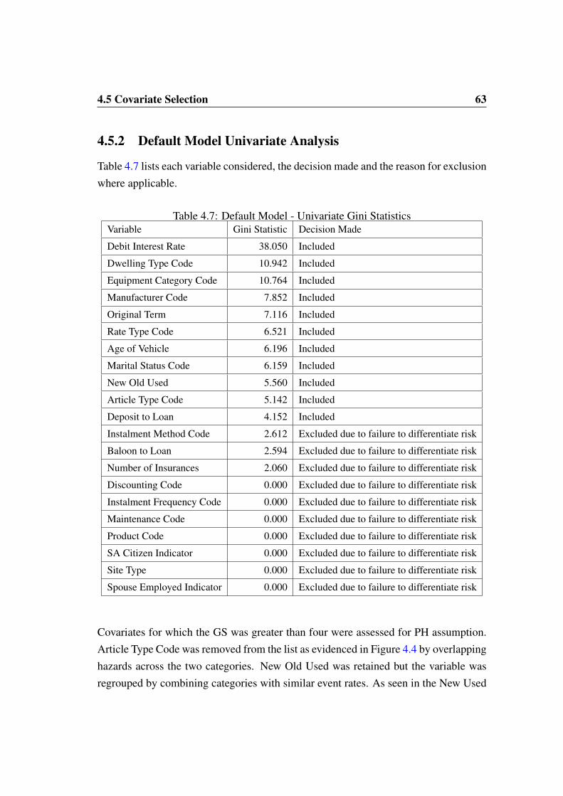
4.5 Covariate Selection 63
4.5.2 Default Model Univariate Analysis
Table 4.7 lists each variable considered, the decision made and the reason for exclusionwhere applicable.
Table 4.7: Default Model - Univariate Gini StatisticsVariable Gini Statistic Decision Made
Debit Interest Rate 38.050 Included
Dwelling Type Code 10.942 Included
Equipment Category Code 10.764 Included
Manufacturer Code 7.852 Included
Original Term 7.116 Included
Rate Type Code 6.521 Included
Age of Vehicle 6.196 Included
Marital Status Code 6.159 Included
New Old Used 5.560 Included
Article Type Code 5.142 Included
Deposit to Loan 4.152 Included
Instalment Method Code 2.612 Excluded due to failure to differentiate risk
Baloon to Loan 2.594 Excluded due to failure to differentiate risk
Number of Insurances 2.060 Excluded due to failure to differentiate risk
Discounting Code 0.000 Excluded due to failure to differentiate risk
Instalment Frequency Code 0.000 Excluded due to failure to differentiate risk
Maintenance Code 0.000 Excluded due to failure to differentiate risk
Product Code 0.000 Excluded due to failure to differentiate risk
SA Citizen Indicator 0.000 Excluded due to failure to differentiate risk
Site Type 0.000 Excluded due to failure to differentiate risk
Spouse Employed Indicator 0.000 Excluded due to failure to differentiate risk
Covariates for which the GS was greater than four were assessed for PH assumption.Article Type Code was removed from the list as evidenced in Figure 4.4 by overlappinghazards across the two categories. New Old Used was retained but the variable wasregrouped by combining categories with similar event rates. As seen in the New Used
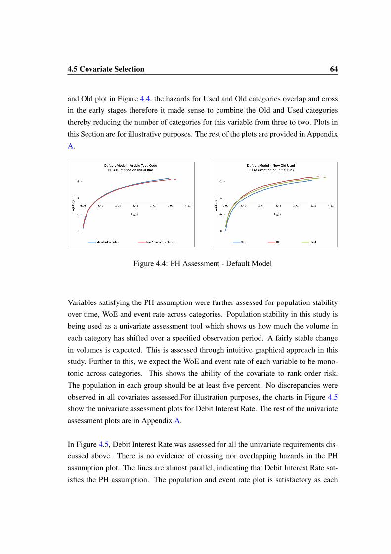
4.5 Covariate Selection 64
and Old plot in Figure 4.4, the hazards for Used and Old categories overlap and crossin the early stages therefore it made sense to combine the Old and Used categoriesthereby reducing the number of categories for this variable from three to two. Plots inthis Section are for illustrative purposes. The rest of the plots are provided in AppendixA.
Figure 4.4: PH Assessment - Default Model
Variables satisfying the PH assumption were further assessed for population stabilityover time, WoE and event rate across categories. Population stability in this study isbeing used as a univariate assessment tool which shows us how much the volume ineach category has shifted over a specified observation period. A fairly stable changein volumes is expected. This is assessed through intuitive graphical approach in thisstudy. Further to this, we expect the WoE and event rate of each variable to be mono-tonic across categories. This shows the ability of the covariate to rank order risk.The population in each group should be at least five percent. No discrepancies wereobserved in all covariates assessed.For illustration purposes, the charts in Figure 4.5show the univariate assessment plots for Debit Interest Rate. The rest of the univariateassessment plots are in Appendix A.
In Figure 4.5, Debit Interest Rate was assessed for all the univariate requirements dis-cussed above. There is no evidence of crossing nor overlapping hazards in the PHassumption plot. The lines are almost parallel, indicating that Debit Interest Rate sat-isfies the PH assumption. The population and event rate plot is satisfactory as each

4.5 Covariate Selection 65
category has a population greater than five percent. The monotonic event rate and theWoE curves show that the variable has the ability to rank order. Population stabilityplot gives an intuitive assessment to show that there are no unreasonable trends in cat-egories across the observation period. With all the conditions satisfied, Debit InterestRate qualifies in the multivariate analysis stage for the default model.
Figure 4.5: Univarite Assessment Plots - Default Model
Note that for each model the visual population stability was assessed over the fullobservation period. However the bars became inconspicuous with too many bars asseen in Figure 4.6, where we illustrate this using the Dwelling Type Code variable.The variable maintained consistent volumes in each category from April 2009 to March2014. For a clearer view the plots trend will shown over the latest two years, from April2012 to March 2014. The rest of the population stability assessment plots are in theAppendix A. No discrepancies were observed.

4.5 Covariate Selection 66
Figure 4.6: Population Stability
4.5.3 Default Model Multivariate Analysis - Cox Regression
Varibles satisfying all the univariate assessment tests were considered for multivariateanalysis. Figure 4.7 summarises results from the multivariate assessment on the basisof the following criteria.
• Variable Importance and VIF Analysis table: Covariates are listed in order oftheir importance in determining default, and the order in which they were enteredinto the model at stepwise regression. Debit Interest Rate is the most significantvariable in the Default model, followed by Dwelling Type Code and the leastimportant is Age of Vehicle. Variable New Old Used was excluded from theanalysis due to a high VIF value which is greater than three, suggesting that itis correlated with one or more of the other predictors, which leads to parameterinstability.
• Model Selection Criteria chart: At each step through stepwise regression, themodel selection criteria are determined. These are the AIC, SBC and -2 Log-likelihood. The most parsimonious model is reflected in the lower values ofthese criteria. However the point at which the graph levels off, gives an indica-tion of where adding more covariates beyond that point will not improve model

4.5 Covariate Selection 67
performance. As the plot levels off at point six, it makes sense to exclude vari-ables added at any point later than the sixth step. This criteria suggested that thevariable Age of Vehicle should be excluded from the analysis at this stage.
• Correlation Matrix: The values in this table complement the analyses in theabove steps. New Old Used is highly correlated with Age of Vehicle (0.7592)and Equipment Category Code (-0.7859). Age of Vehicle is also highly cor-related with Equipment Category Code (-0.5967). This means dropping Age ofVehicle does not lead to information loss as this information is already containedin Equipment Category Code and New Old Used.
Figure 4.7: Multivariate Analysis - Default Model
Taking all these criteria suggests that the most significant predictors for the defaultmodel are the ones listed in Table 4.8. Recall that for each covariate, the final categorieswere reached through a thorough univariate assessment as discussed extensively inSection 4.5.2. As a result each variable making into the final model is provided inTable 4.8 with a description of each of the categories.

4.5 Covariate Selection 68
Table 4.8: Final Covariates - Default Model
Variable Category Value Description
Debit Interest Rate
1 Less than 11 Less than 11
2 [11,14.2) Greater than or equal to 11
but less than 14.2
3 14.2+ Greater than 14.2
Deposit to Loan1 No deposit paid No deposit paid
2 Deposit paid Deposit paid
Dwelling Type Code
1 Tenant Customer is a tenant
2 Parents Customer living with par-
ents
3 Owner Customer owns a residen-
tial property
Equipment Category Code
1 Used Vehicles Demo and Preowned vehi-
cles
2 New Vehicles Brand new Vehicles
Marital Status Code
1 Married The customer is married
2 Other Includes Single, Divorced,
Widowed customers
4.5.4 Early Settlement Model Univariate Analysis
Univariate assessment conducted in the default model was adopted for the ES model.Variables were grouped using the interactive grouping node in SAS R© Enterprise Miner.The first set of categories were checked for logic and ability to rank order, where theconditions were not met, variables were then re-grouped manually, according to mean-ing, volumes and event rate. All covariates were assessed using GS to determine theirability to differentiate risk. For ES, all variables were assessed for PH assumptionresulting in further exclusions, regrouping and retention of satisfactorily grouped co-variates. Table 4.9 lists each variable considered and the decision made. Exclusions

4.5 Covariate Selection 69
were made due to failure of the covariate to differentiate risk.
Table 4.9: Early Settlement Model - Univariate Gini StatisticsVariable Gini Statistic Decision Made
Original Term 20.982 Included
Ballon to Loan 18.117 Included
Deposit to Loan 16.247 Included
Equipment Category Code 14.406 Included
Age of Vehicle 12.769 Included
New Old Used 11.858 Included
Dwelling Type Code 9.952 Included
Marital Status Code 8.411 Included
Number of Insurances 8.053 Included
Rate Type Code 7.585 Included
Manufacturer Code 6.550 Included
Article Type Code 4.605 Included
Debit Interest Rate 4.321 Included
Instalment Method Code 0.000 Excluded
Discounting Code 0.000 Excluded
Instalment Frequency Code 0.000 Excluded
Maintenance Code 0.000 Excluded
Product Code 0.000 Excluded
SA Citizen Indicator 0.000 Excluded
Site Type 0.000 Excluded
Spouse Employed Indicator 0.000 Excluded
Covariates passing the GS were assessed for PH assumption. Variables were regroupedwhere necessary. The PH plots used to select predictors are provided in AppendixA.3. Covariates which were excluded due to failure to satisfy PH assumption in theES model are: Article Type Code, Manufacturer Code, Rate Type Code, Number ofInsurances, Marital Status Code and Balloon to Loan. Variables passing the PH as-

4.5 Covariate Selection 70
sumption were further assessed for population stability over time. The WoE and eventrate should be monotonic across groups. The population in each group should be atleast 5 percent. No discrepancies were observed. The rest of the univariate assessmentplots are in the Appendix A.3.
4.5.5 Early Settlement Model Multivariate Analysis - Cox Regres-sion
Varibles satisfying all the univariate assessment tests were considered for multivariateanalysis. As in the Default model, the bucket combination with the largest populationwas manually selected and used as the baseline. Figure 4.8 summarises results fromthe multivariate assessment.
• Variable Importance and VIF Analysis table: Equipment Category Code is thestrongest variable in the ES model, followed by Debit Interest Rate and the leastimportant is New Old Used. The variables Age of Vehicle and New Old Usedwere excluded from the analysis due to their high VIF value which is greaterthan 3 in each case. This was done to avoid parameter instability.
• Model Selection Criteria chart: The model selection criteria were determined.The AIC, SBC and -2 Loglikelihood plots level off at point 6, it makes senseto exclude variables added at any point later than the 6th step. This criteriasuggests that the variable New Old Used should be excluded from the analysisat this stage. This complements information in the VIF analysis and correlationmatrix as well.
• Correlation Matrix: Variables with high correlation were already excluded dueto high VIF. Age of Vehicle and Equipment Category Code (-0.7038). New OldUsed is highly correlated with Equipment Category Code (0.8468). DroppingAge of Vehicle does not lead to information loss as this information is alreadycontained in Equipment Category Code.
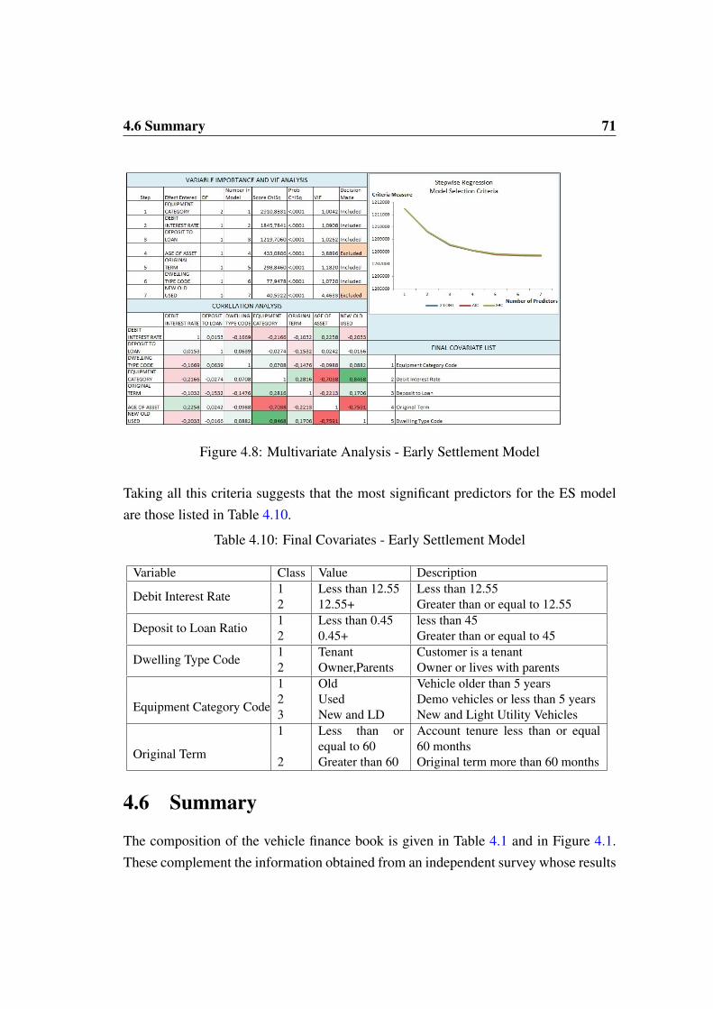
4.6 Summary 71
Figure 4.8: Multivariate Analysis - Early Settlement Model
Taking all this criteria suggests that the most significant predictors for the ES modelare those listed in Table 4.10.
Table 4.10: Final Covariates - Early Settlement Model
Variable Class Value Description
Debit Interest Rate1 Less than 12.55 Less than 12.552 12.55+ Greater than or equal to 12.55
Deposit to Loan Ratio1 Less than 0.45 less than 452 0.45+ Greater than or equal to 45
Dwelling Type Code1 Tenant Customer is a tenant2 Owner,Parents Owner or lives with parents
Equipment Category Code
1 Old Vehicle older than 5 years2 Used Demo vehicles or less than 5 years3 New and LD New and Light Utility Vehicles
Original Term
1 Less than orequal to 60
Account tenure less than or equal60 months
2 Greater than 60 Original term more than 60 months
4.6 Summary
The composition of the vehicle finance book is given in Table 4.1 and in Figure 4.1.These complement the information obtained from an independent survey whose results
4.6 Summary 72
are summarised in a biplot in Figure 1.1 of Chapter 1 and the brands appearing in thebiplot are indeed the “popular” brands of the South African automobile market. Overa 5 year observation period, individual accounts were tracked every month from thepoint of entry to the point of exit into either default, ES or to the termination of studyat the end of March 2014. Covariate selection process was thoroughly done and all thecovariates selected satisfied the conditions required in a univariate analysis. Variablessatisfying multivariate approaches were then used in fitting the models. Further detailis provided in Chapter 5.

Chapter 5
Results and Analysis
5.1 Introduction
Credit risk refers to potential loss associated with loans issued to consumers due to bor-rower’s failure to meet contractual obligations. Among other risks (e.g liquidity buffer,operational and market risks), credit risk is the most significant source of regulatorycapital demand. In order to hold adequate capital against credit risk, financial insti-tutions should adopt the use of advanced statistical capital models to calculate capitaldemand. To comply with the requirements of the Basel Accord, the organisation set upinternal model building standards detailed in Section 5.7. These were adopted in thisstudy, to assess adequacy and accuracy of each model. Statistical assumptions of themodels built were verified. Model comparisons were made and the results presentedgraphically and numerically. Analyses were conducted to determine the methodologystriving to perform better for a consumer credit cohort data in the presence of compet-ing risks and long term survivors.
5.2 Model Fitting
In fitting all the models, it was opted to manually select the categories to be consideredas the baseline rather than opting for an automatic selection. This was done to optimisethe volumes in the baseline to ensure maximum statistical significance for as manyvariables as possible. Therefore the category combination with the largest population

5.3 Logistic Regression 74
was manually selected and used as the baseline for each event. For each model, thecategory combination giving the highest population is given in Table 5.1.
Table 5.1: Baseline PopulationDefault Model ES Model
Variable Category Variable CategoryDebit Interest Rate 2 Debit Interest Rate 1
Deposit to Loan Ratio 1 Deposit to Loan Ratio 1
Dwelling Type Code 1 Dwelling Type Code 2
Equipment Category Code 1 Equipment Category Code 3
Marital Status Code 1 Original Term 2
Following the model building process, each model variant was fitted. Logistic regres-sion was fitted for each event type. Cox PH regression was fitted for each event typeas well. No discrepancies were observed in all models. For each covariate, categoryspecific p-values indicated that all variables were significant at granular level.
5.3 Logistic Regression
Models were fitted separately for each event type. In each case, accounts used formodel development were allowed at least 48 months to perform. This is the “waiting”performance period to maturity, required for the purposes of LR. The account-levelprobabilities were calculated based on the event observed at month 48. Results andanalyses are provided below.
5.3.1 Default Model Multivariate Analysis - Logistic Regression
A stepwise multivariate analysis was conducted to select the final covariates and cat-egories for use in the default Logistic regression model. All covariates met the 0.05significance level for entry into the model and the order of importance is given in Table5.2.
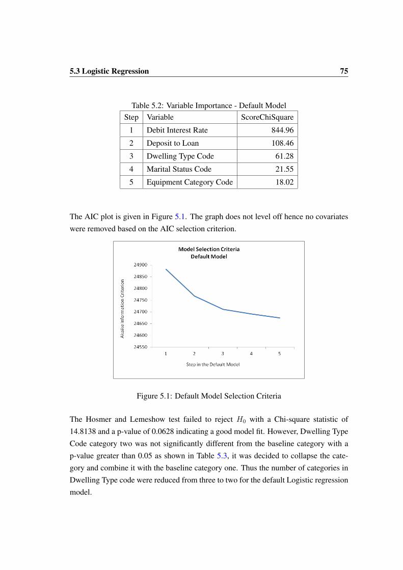
5.3 Logistic Regression 75
Table 5.2: Variable Importance - Default ModelStep Variable ScoreChiSquare
1 Debit Interest Rate 844.96
2 Deposit to Loan 108.46
3 Dwelling Type Code 61.28
4 Marital Status Code 21.55
5 Equipment Category Code 18.02
The AIC plot is given in Figure 5.1. The graph does not level off hence no covariateswere removed based on the AIC selection criterion.
Figure 5.1: Default Model Selection Criteria
The Hosmer and Lemeshow test failed to reject H0 with a Chi-square statistic of14.8138 and a p-value of 0.0628 indicating a good model fit. However, Dwelling TypeCode category two was not significantly different from the baseline category with ap-value greater than 0.05 as shown in Table 5.3, it was decided to collapse the cate-gory and combine it with the baseline category one. Thus the number of categories inDwelling Type code were reduced from three to two for the default Logistic regressionmodel.

5.3 Logistic Regression 76
Table 5.3: Logistic Stepwise Regression - Default ModelVariable Class Estimate Odds Ratio P Value
Intercept -2.0826
Debit Interest Rate
1 -0.5969 0.5504 <.0001
2 0.0000 1.0000
3 0.7293 2.0737 <.0001
Deposit to Loan1 0.0000 1.0000
2 -0.4752 0.6217 <.0001
Dwelling Type Code
1 0.0000 1.0000
2 -0.0285 0.9718 0.5650
3 -0.2514 0.7776 <.0001
Equipment Category Code1 0.0000 1.0000
2 -0.1906 0.8264 <.0001
Marital Status Code1 0.0000 1.0000
2 -0.1731 0.8409 <.0001
5.3.2 Default Model - Logistic Regression
The maximum likelihood estimates are provided in Table 5.4. The parameter estimatesfor the baseline population are all valued at 0 as the baseline is used as the empiricalreference population, and should not be influenced by the effect of covariates. The oddsratio is obtained by exponentiating the corresponding parameter estimate for each cat-egory. Subsequently, the odds ratios of the baseline population take up the value of1. Thus, the movement in odds ratio from the baseline is relative to the movement inparameter estimates of the respective category.
Odds are calculated based on probabilities and they range between 0 and +∞. Theygive us a ratio of the probability of default versus the probability of non default ineach category. Reading from Table 5.4, the ratio of odds of defaulting for accountswith a Debit Interest Rate of 14.2 versus those with [11,14.2) is 2.0792 to 1. Thisshows the extent to which accounts with Debit Interest Rate of 14.2 are more prone
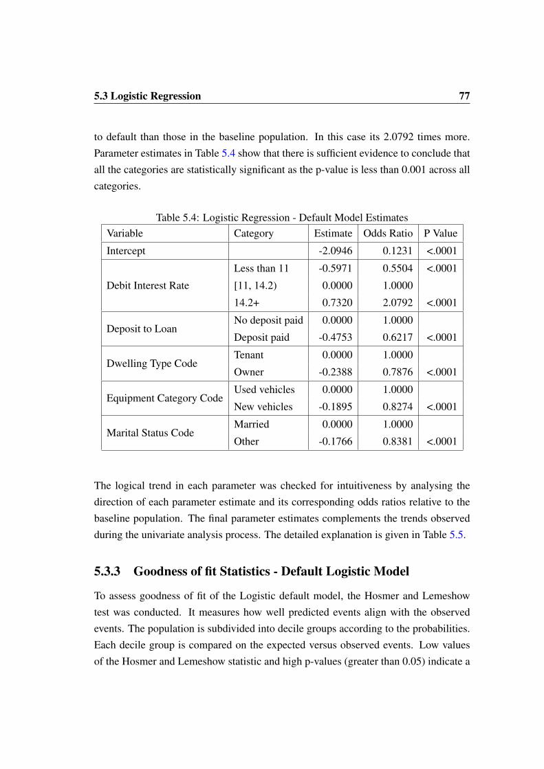
5.3 Logistic Regression 77
to default than those in the baseline population. In this case its 2.0792 times more.Parameter estimates in Table 5.4 show that there is sufficient evidence to conclude thatall the categories are statistically significant as the p-value is less than 0.001 across allcategories.
Table 5.4: Logistic Regression - Default Model EstimatesVariable Category Estimate Odds Ratio P Value
Intercept -2.0946 0.1231 <.0001
Debit Interest Rate
Less than 11 -0.5971 0.5504 <.0001
[11, 14.2) 0.0000 1.0000
14.2+ 0.7320 2.0792 <.0001
Deposit to LoanNo deposit paid 0.0000 1.0000
Deposit paid -0.4753 0.6217 <.0001
Dwelling Type CodeTenant 0.0000 1.0000
Owner -0.2388 0.7876 <.0001
Equipment Category CodeUsed vehicles 0.0000 1.0000
New vehicles -0.1895 0.8274 <.0001
Marital Status CodeMarried 0.0000 1.0000
Other -0.1766 0.8381 <.0001
The logical trend in each parameter was checked for intuitiveness by analysing thedirection of each parameter estimate and its corresponding odds ratios relative to thebaseline population. The final parameter estimates complements the trends observedduring the univariate analysis process. The detailed explanation is given in Table 5.5.
5.3.3 Goodness of fit Statistics - Default Logistic Model
To assess goodness of fit of the Logistic default model, the Hosmer and Lemeshowtest was conducted. It measures how well predicted events align with the observedevents. The population is subdivided into decile groups according to the probabilities.Each decile group is compared on the expected versus observed events. Low valuesof the Hosmer and Lemeshow statistic and high p-values (greater than 0.05) indicate a

5.3 Logistic Regression 78
Table 5.5: Intuitiveness of Signs of the Default Model - Logistic Regression
Variable Relation to
Baseline
Explanation
Debit Interest Rate Positive From table 5.4, the odds ratios show an increas-
ing trend over the rank ordered categories. The
odds of 14.2+ category are 1.08 higher than the
odds of category [11,14.2). This implies that the
rate of default increases with increasing debit
interest rate. Thus, more expensive loans due to
high interest rate are more prone to default than
those with lower interest rate.
Dwelling Type Code Negative The odds of owners are 22% lower than the
odds of tenants. Home owners have a lower
probability of default than tenants. The greater
the equity associated with customers, the lower
the probability of default.
Deposit to Loan Ratio Negative The odds of deposit payers are 38% lower than
the odds of customers who did not pay a de-
posit. The rate of default decreases with in-
creasing deposit paid. If a deposit is paid, the
capital loan amount reduces and the cost of bor-
rowing becomes cheaper and thus the rate of
default is minimal where the deposit has been
paid.
Equipment Category
Code
Negative The odds of new vehicles are 18% lower than
the odds of new vehicles. Old vehicles are as-
sociated with higher default rate compared to
new vehicles as the demand for ageing vehicles
diminishes.
Marital Status Code Negative The odds of married customers are 17% higher
than the odds of the unmarried. Marriage comes
with greater responsibilities, customers become
more prone to default on loans.

5.3 Logistic Regression 79
good fit of the observed versus predicted event rates. For the default model, the Chi-square statistic of 15,2447 was obtained, with a corresponding p-value of 0,0546. Thisindicates that this model does fit the data. The Hosmer and Lemeshow test partitionsdata into decile groups according to risk levels. Results in Table 5.6 indicate that theobserved and expected rates of default are similar by population deciles.
Table 5.6: The Hosmer and Lemeshow Partition - Default ModelGroup Total Population Events
Observed
Events
Expected
Nonevents
Observed
Nonevents
Expected
1 3643 110 124.73 3533 3518.27
2 4298 193 198.42 4105 4099.58
3 3900 217 231.39 3683 3668.61
4 5717 429 422.23 5288 5294.77
5 3634 309 316.09 3325 3317.91
6 4247 424 398.82 3823 3848.18
7 3548 414 401.45 3134 3146.55
8 4216 626 602.00 3590 3614.00
9 4499 799 772.51 3700 3726.49
10 2298 415 468.36 1883 1829.64
For each risk group, the actual versus observed event rates were calculated based onthe total population. This was done to determine the ability of the model to rank orderrisk and to establish how accurate the model is, in predicting risk. Thus the values ofactual and expected event rates were plotted across range of the risk. For the modelsto be accurate, the actual versus expected plots should not deviate significantly fromthe 45 degree diagonal. To check the ability of the model to rank order risk, the pointsshould lie in increasing order of the risk group. Accuracy and rank ordering metricswere determined for both development and validation data sets. The accuracy plots areprovided in Figure 5.2. No discrepancies were observed as all the points in both datasets are satisfactorily rank ordered and they all lie close to the 45 degree diagonal.

5.3 Logistic Regression 80
Figure 5.2: Accuracy Plots Default Model
5.3.4 Early Settlement Model Multivariate Analysis - Logistic Re-gression
As in the default model, a stepwise multivariate analysis was conducted to select thefinal covariates and categories for the ES Logistic regression model. Original Termfailed to meet the 0.05 significance level for entry into the model at stepwise regres-sion stage, hence it was dropped. The remaining covariates are listed in Table 5.7.

5.3 Logistic Regression 81
Table 5.7: Variable Importance - ES Model
Step EffectEntered ScoreChiSq
1 Equipment Category Code 647.69
2 Debit Interest Rate 501.65
3 Deposit to Loan 271.44
4 Dwelling Type Code 10.26
The selection criteria plot of the ES model is provided in Figure 5.3. As seen in theplot, the graph does not level off, thus no further covariates were removed.
Figure 5.3: Early Settlement Model Selection Criteria
The Hosmer and Lemeshow test was conducted and we obtained a Chi-square statisticof 66.9723 and a p-value less than 0.05 leading to the rejection of the null hypothe-sis. To correct model misfit, it was decided to re-run the stepwise regression using allpossible two way interaction terms. Insignificant categories were removed until a finalmodel with some interaction terms, was achieved. The descriptions of the Early Settle-ment covariates and their corresponding categories are detailed in Table 4.10, with theexception of Original Term. The final categories and interaction terms are provided inChapter 5, Table 5.8.
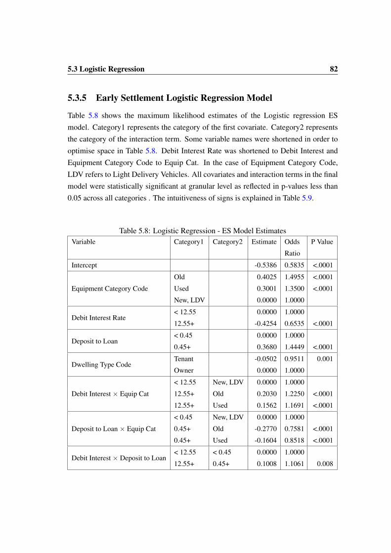
5.3 Logistic Regression 82
5.3.5 Early Settlement Logistic Regression Model
Table 5.8 shows the maximum likelihood estimates of the Logistic regression ESmodel. Category1 represents the category of the first covariate. Category2 representsthe category of the interaction term. Some variable names were shortened in order tooptimise space in Table 5.8. Debit Interest Rate was shortened to Debit Interest andEquipment Category Code to Equip Cat. In the case of Equipment Category Code,LDV refers to Light Delivery Vehicles. All covariates and interaction terms in the finalmodel were statistically significant at granular level as reflected in p-values less than0.05 across all categories . The intuitiveness of signs is explained in Table 5.9.
Table 5.8: Logistic Regression - ES Model EstimatesVariable Category1 Category2 Estimate Odds
Ratio
P Value
Intercept -0.5386 0.5835 <.0001
Equipment Category Code
Old 0.4025 1.4955 <.0001
Used 0.3001 1.3500 <.0001
New, LDV 0.0000 1.0000
Debit Interest Rate< 12.55 0.0000 1.0000
12.55+ -0.4254 0.6535 <.0001
Deposit to Loan< 0.45 0.0000 1.0000
0.45+ 0.3680 1.4449 <.0001
Dwelling Type CodeTenant -0.0502 0.9511 0.001
Owner 0.0000 1.0000
Debit Interest × Equip Cat
< 12.55 New, LDV 0.0000 1.0000
12.55+ Old 0.2030 1.2250 <.0001
12.55+ Used 0.1562 1.1691 <.0001
Deposit to Loan × Equip Cat
< 0.45 New, LDV 0.0000 1.0000
0.45+ Old -0.2770 0.7581 <.0001
0.45+ Used -0.1604 0.8518 <.0001
Debit Interest × Deposit to Loan< 12.55 < 0.45 0.0000 1.0000
12.55+ 0.45+ 0.1008 1.1061 0.008

5.3 Logistic Regression 83
Table 5.9: Intuitiveness of Signs of the Early Settlement Model - Logistic Regression
Variable Relation to
baseline
Explanation
Debit Interest Rate Negative The odds of customers whose interest rate
is 12.55+ settling early is 35% lower than
the odds of customers whose interest rate
is lower than 12.55. It is difficult to set-
tle early on expensive loans hence the ES
odds are lower in the higher category of
debit interest rate.
Deposit to Loan Ratio Positive The ES odds of customers who paid de-
posit to loan ratio of 0.45+ are 44% higher
than the odds of customers who paid less
than 0.45. If a deposit amount is paid,
it reduces the capital amount of the loan
and it becomes easier to settle the balance
early on lower capital base.
Dwelling Type Code Negative The odds of settling early are 5% lower
for home owners than tenants. Home
owners have a higher tendency to settle
early than tenants. The greater the equity
associated with customers, the higher the
probability of ES as they perhaps shift fo-
cus to longer term home loans.
Equipment Category Code Positive The odds to settle early are 35% higher in
used vehicles compared to new and 49%
higher in old vehicles than new. Old vehi-
cles have a highest probability of ES com-
pared to Used and New. As customers up-
grade to new vehicle models, settlement
occurs most oftenly on old vehicles.
Debit Int × Equipment Cat Positive Old vehicles coupled with high interest
rate have the highest odds of ES as there
is higher urge to avoid high interest and
dispose old asset.
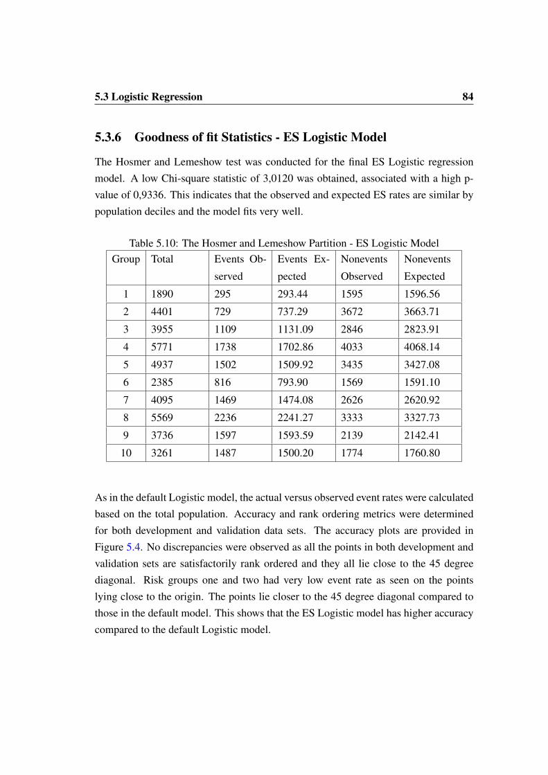
5.3 Logistic Regression 84
5.3.6 Goodness of fit Statistics - ES Logistic Model
The Hosmer and Lemeshow test was conducted for the final ES Logistic regressionmodel. A low Chi-square statistic of 3,0120 was obtained, associated with a high p-value of 0,9336. This indicates that the observed and expected ES rates are similar bypopulation deciles and the model fits very well.
Table 5.10: The Hosmer and Lemeshow Partition - ES Logistic ModelGroup Total Events Ob-
served
Events Ex-
pected
Nonevents
Observed
Nonevents
Expected
1 1890 295 293.44 1595 1596.56
2 4401 729 737.29 3672 3663.71
3 3955 1109 1131.09 2846 2823.91
4 5771 1738 1702.86 4033 4068.14
5 4937 1502 1509.92 3435 3427.08
6 2385 816 793.90 1569 1591.10
7 4095 1469 1474.08 2626 2620.92
8 5569 2236 2241.27 3333 3327.73
9 3736 1597 1593.59 2139 2142.41
10 3261 1487 1500.20 1774 1760.80
As in the default Logistic model, the actual versus observed event rates were calculatedbased on the total population. Accuracy and rank ordering metrics were determinedfor both development and validation data sets. The accuracy plots are provided inFigure 5.4. No discrepancies were observed as all the points in both development andvalidation sets are satisfactorily rank ordered and they all lie close to the 45 degreediagonal. Risk groups one and two had very low event rate as seen on the pointslying close to the origin. The points lie closer to the 45 degree diagonal compared tothose in the default model. This shows that the ES Logistic model has higher accuracycompared to the default Logistic model.

5.3 Logistic Regression 85
Figure 5.4: Accuracy Plots Early Settlement Model
Both LR models were fitted satisfactorily. For each model the ROCs curves were cal-culated and the corresponding area under the curves were determined. The model GSswere also calculated to determine the ability of each model to differentiate risk. Thesewere then compared to the those obtained in the corresponding Cox PH models to de-termine the methodology striving to perform better given lifetime data in a consumercredit setting in the presence of competing risks and long term survivors. More detailis provided in Section 5.6.
5.4 Cox PH Regression 86
5.4 Cox PH Regression
Unlike the Logistic development data selection process, the Cox regression model doesnot consider a “waiting” period. All accounts are eligible for inclusion in the develop-ment. Accounts recently entered into the study also play a very important role. If notabsorbed into any of the event then they can be classified as censored and form partof the risk set according to time spent in study. Two cause specific PH models werefitted separately for each event. A CIC was calculated in each case to determine themarginal probabilities of an event happening at a fixed workout period of 48 months inthe presence of competing risks and long term survivors.
5.4.1 Long Term Survivors
As evidenced by the empirical KM curve in Figure 5.5, the overall survival plot levelsoff at non zero values. This indicates that the bulk of accounts are not susceptible tothe events of interest. It makes business sense as most of the customers on the vehiclefinance book are good customers and statistically, that prompts heavy censoring atthe end of the study. A proportion (p) of good customers is chosen such that theoverall survival curve levels of to p. In this case the minimum value of the survivalcurve was selected as p. Thus p = 0.49179045. Using the Cure model approach, thesurvival functions will be adjusted to allow for long term survivors. The proportion ofsusceptible population A = p and that of non-susceptible population B = 1 − p. Thesurvivor function of the entire population (A + B) is given by:
S(t) = (1− p) + pSA(t) (5.1)
where SA(t) is the survivor function of population A. For each model, the hazardfunction was derived from the survivor function and the corresponding CIC’s werecalculated. The final models were tested on the validation set.

5.4 Cox PH Regression 87
Figure 5.5: Kaplain Meier Survival Curve
5.4.2 Analysis of The Hazard Functions
In survival analysis, we assume that neither of the events can happen at the point ofentry. Thus the survival probability at time 0 is equal to 1 and conversely, the hazardfunction at time 0 is equal to 0. As the survival time in this study is discrete, weexpect the events to start occurring at month 1 onwards. Figures 5.7 and 5.6 show theempirical probability mass and hazard functions for ES and default events respectively.For both events, the functions start at zero as there are no events recorded at the entrypoints. The probability mass function of ES is the number of accounts settling earlyat any t, from 0 to 48, relative to the total number of early settlements in the book. Itis a function of the total number of ES events which shows the probability distributionof the early settlement event over time. The probability distribution functions weredetermined for both events. The hazard function is the instantaneous rate of occurrenceof an event. This is a function of the accounts at risk at any t. The hazard functionswere calculated and plotted for each event as well.
5.4.2.1 Default Event
With reference to Figure 5.6, the probability mass function of the default event in-creases sharply in the first 18 months of the loans. The same trend is reflected in thecorresponding hazard function which increases sharply up to 18 months and gener-

5.4 Cox PH Regression 88
ally stabilises beyond the 18-month point. This is due to the fact that at the point ofapplication, the selected customers have low risk of default but, as time goes on, cus-tomers experience various social and economic events leading to default and the riskof default increases. This trend is experienced in the first 1 and half years of loans forthe vehicle finance product. As the accounts grow older than 18 months, the rate ofdefault decreases, accounts passing this point have a lower chance of default. This isattributable to the fact that most customers improve their financial status with time andthe original repayment amount becomes insignificant with time and hence the chanceof default diminishes as time approaches 48 months.
Figure 5.6: Default Event - Hazard Function
5.4.2.2 Early Settlement Event
The probability mass function in Figure 5.7 increases steadily in the first 18 months,decreases at a steady rate beyond 18 months and diminishes towards 48 months. Thisis also reflected in the hazard function that is on an increasing trend for the same 18months and rather stabilizes later. For the first 1 and half years from the entry point, therisk of early settlement increases with increasing time. As the vehicle ages, the chancesof early settlement increases as customers upgrade to new vehicle models. However, asthe accounts approach maturity, the risk of early settlement lessens as it becomes easierto complete the originally agreed term of repayment and customers rather complete therepayment normally instead of settling early, to avoid penalty charges associated withthe event.
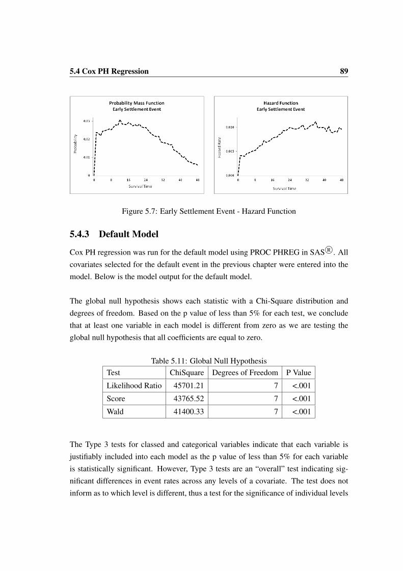
5.4 Cox PH Regression 89
Figure 5.7: Early Settlement Event - Hazard Function
5.4.3 Default Model
Cox PH regression was run for the default model using PROC PHREG in SAS R©. Allcovariates selected for the default event in the previous chapter were entered into themodel. Below is the model output for the default model.
The global null hypothesis shows each statistic with a Chi-Square distribution anddegrees of freedom. Based on the p value of less than 5% for each test, we concludethat at least one variable in each model is different from zero as we are testing theglobal null hypothesis that all coefficients are equal to zero.
Table 5.11: Global Null HypothesisTest ChiSquare Degrees of Freedom P Value
Likelihood Ratio 45701.21 7 <.001
Score 43765.52 7 <.001
Wald 41400.33 7 <.001
The Type 3 tests for classed and categorical variables indicate that each variable isjustifiably included into each model as the p value of less than 5% for each variableis statistically significant. However, Type 3 tests are an “overall” test indicating sig-nificant differences in event rates across any levels of a covariate. The test does notinform as to which level is different, thus a test for the significance of individual levels
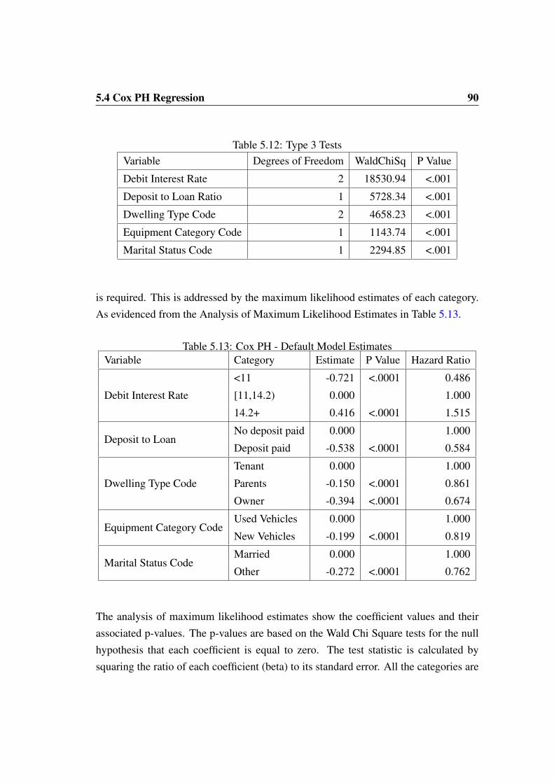
5.4 Cox PH Regression 90
Table 5.12: Type 3 TestsVariable Degrees of Freedom WaldChiSq P Value
Debit Interest Rate 2 18530.94 <.001
Deposit to Loan Ratio 1 5728.34 <.001
Dwelling Type Code 2 4658.23 <.001
Equipment Category Code 1 1143.74 <.001
Marital Status Code 1 2294.85 <.001
is required. This is addressed by the maximum likelihood estimates of each category.As evidenced from the Analysis of Maximum Likelihood Estimates in Table 5.13.
Table 5.13: Cox PH - Default Model EstimatesVariable Category Estimate P Value Hazard Ratio
Debit Interest Rate
<11 -0.721 <.0001 0.486
[11,14.2) 0.000 1.000
14.2+ 0.416 <.0001 1.515
Deposit to LoanNo deposit paid 0.000 1.000
Deposit paid -0.538 <.0001 0.584
Dwelling Type Code
Tenant 0.000 1.000
Parents -0.150 <.0001 0.861
Owner -0.394 <.0001 0.674
Equipment Category CodeUsed Vehicles 0.000 1.000
New Vehicles -0.199 <.0001 0.819
Marital Status CodeMarried 0.000 1.000
Other -0.272 <.0001 0.762
The analysis of maximum likelihood estimates show the coefficient values and theirassociated p-values. The p-values are based on the Wald Chi Square tests for the nullhypothesis that each coefficient is equal to zero. The test statistic is calculated bysquaring the ratio of each coefficient (beta) to its standard error. All the categories are

5.4 Cox PH Regression 91
statistically significantly different from the baseline groups in the final model.
The hazard ratio gives the measure of effect of explanatory variables. The correspond-ing measure of the effect in a Logistic regression environment is the odds ratio. Hazardratios are calculated based on instantaneous rate of default happening in predefinedsubgroups, in this case the reference group and each of the categories at any t, giventhat the subject survived up to t.
Given parameter estimates, hazard ratios can be obtained by exponentiating parameterestimates in each category. This is analogous to the calculation of odds ratios in Logis-tic regression. Their values range between 0 and +∞ as well. The baseline populationhave 0 parameter estimates with hazard ratios of 1. For values of HR less than 1, itimplies the category has less risk of default than the baseline and vice versa for HRvalues greater than 1.
Reading from Table 5.13, the ratio of hazards of defaulting for accounts with a DebitInterest Rate of 14.2 versus those with [11,14.2) is 1.515 to 1. This shows the extent towhich accounts with Debit Interest Rate of 14.2 are more prone to default than thosein the baseline population. In this case its 1.515 times more. We look at the directionof estimates and the corresponding hazard ratios to determine intuitiveness and relateto business sense in Section 5.4.4.
5.4.4 Intuitiveness of Signs - Default Cox PH Model
The logical trend in each parameter is checked for intuitiveness by analysing the direc-tion of each parameter estimate relative to the baseline. The final parameter estimatescomplements the trends observed during the univariate analysis process. The detailedexplanation is given in Table 5.14.

5.4 Cox PH Regression 92
Table 5.14: Intuitiveness of Signs of the Default Model
Variable Relation to
Baseline
Explanation
Debit Interest Rate Positive The hazards of customers with Debit In-
terest of 14+ are 50% higher than those in
[11,14.2). Default rate increases with in-
creasing debit interest rate. Higher inter-
est rate implies more expensive loans and
the accounts in that category have higher
probability of default.
Dwelling Type Code Negative The hazards of default of home own-
ers and customers living with parents are
33% and 14% lower than tenants respec-
tively. Tenants have a higher probabil-
ity of default than home owners and cus-
tomers living with parents. The greater
the equity associated with customers, the
lower the probability of default.
Deposit to Loan Ratio Negative The default hazards of deposit payers are
42% less than deposit non payers’ haz-
ards. The rate of default decreases with
increasing deposit paid. If a deposit is
paid, the capital loan amount reduces and
the cost of borrowing becomes cheaper
and thus the rate of default is minimal
where the deposit has been paid.
Equipment Category Code Negative Old vehicles have 18% higher hazards
of default than new vehicles. This im-
plies that old vehicles are associated with
higher default rate as the demand for age-
ing vehicles diminishes.
Marital Status Code Negative The hazards of default for married cus-
tomers are 24% higher than the unmar-
ried because marriage comes with greater
responsibilities, customers become more
prone to default on loans.

5.4 Cox PH Regression 93
5.4.5 Goodness of Fit Statistics - Cox PH Default Model
The accuracy measures were calculated for the Cox default model. This was performedon both the development and validation data sets. Accounts were ranked separately foreach data set into deciles based on their default cumulative probabilities at month 48.For each decile group the actual and expected observations were determined. Thedefault rate in each group was determined based on the total volumes. For the modelsto be accurate, the actual versus expected plots should not deviate significantly fromthe 45 degree diagonal. The accuracy plots for the default model are provided in Figure5.8. No discrepancies were observed.
Figure 5.8: Accuracy Plots Default Cox Model

5.4 Cox PH Regression 94
5.4.6 Early Settlement Model
Cox PH regression was run for the ES model using PROC PHREG in SAS R©. All co-variates selected for the ES event in the previous chapter were entered into the model.With p values of less than 0.001 for each level, there is sufficient evidence to concludethat at granular level, all the covariates are significant. Following is the ES model out-put.
The global null hypothesis shows each statistic with a Chi-Square distribution anddegrees of freedom. Based on the p value of less than 5% for each test, we concludethat at least one variable in each model is different from zero as we are testing theglobal null hypothesis that all coefficients are equal to zero.
Table 5.15: Globall Null HypothesisTest ChiSquare Degrees of Freedom P Value
Likelihood Ratio 6335.92 6 <.001
Score 6388.02 6 <.001
Wald 6293.77 6 <.001
The Type 3 tests for classed and categorical variables indicate that each variable isjustifiably included into the ES model as the p value of less than 5% for each variableis statistically significant.
Table 5.16: Type 3 TestsVariable Degrees of Freedom WaldChiSq P Value
Debit Interest Rate 1 1671.29 <.001
Deposit to Loan Ratio 1 989.42 <.001
Dwelling Type Code 1 60.88 <.001
Equipment Category Code 2 2950.09 <.001
Original Term 1 333.79 <.001
The analysis of maximum likelihood estimates, shows the coefficient vales and their as-sociated p values. As evidenced from the Analysis of Maximum Likelihood Estimates

5.4 Cox PH Regression 95
Table 5.17: Cox PH - Early Settlement Model EstimatesVariable Category Estimate P Value HazardRatio
Debit Interest Rate<12.55 0.000 1.000
12.5+ -0.384 <.0001 0.681
Deposit to Loan<0.45 0.000 1.000
0.45+ 0.378 <.0001 1.460
Dwelling Type CodeTenant -0,078 <.0001 0.925
Owner, Parents 0.000 1.000
Equipment Category Code
Old 0.617 <.0001 1.854
Used 0.463 <.0001 1.589
New, LDV 0.000 1.000
Original Term≤ 60 0.180 <.0001 1.197
60+ 0.000 1.000
in Table 5.17, all the levels are statistically significantly different from the baselinegroups in the final with p-values less than 0.05.
5.4.7 Intuitiveness of Signs - Early Settlement Model
As in all the models discussed above, the ES Cox regression models was also analysedfor intuitiveness of signs. More detail is provided in Table 5.18. The logical trendin each covariate was determined. Again in the ES Cox model, the final parameterestimates complements the trends observed during the univariate analysis process.

5.4 Cox PH Regression 96
Table 5.18: Intuitiveness of Signs of the Early Settlement Model
Variable Relation to
Baseline
Explanation
Debit Interest Rate Negative The hazards of ES of customers with
12.5+ interest rate are 32% lower than
those with debit interest rate less than
12.55. Thus, ES rate decreases as debit
interest rate increases. The greater the in-
terest rate the lesser the probability of ES.
It is easier to settle early on cheaper loans
with lower interest rate.
Deposit to Loan Ratio Positive The hazards of customers with deposit to
loan ratio of 0.45+ are 46% higher than
those with deposit to loan ratio less than
0.45. The ES rate increases with increas-
ing amount of deposit paid. If a de-
posit amount is paid, it reduces the capital
amount of the loan and it becomes easier
to settle the balance early.
Dwelling Type Code Negative Tenants have 7% lower hazards of ES
than home owners. The greater the equity
associated with customers, the higher the
ES probability.
Equipment Category Code Positive Old and Used vehicles have 85% and 58%
higher hazards than New, LDV’s respec-
tively. As customers upgrade to new vehi-
cle models, settlement occurs oftenly on
old and used vehicles.
Original Term Negative With a negative trend in hazard ratios,
that is the hazards of 60+ are 20% lower
than those in less than 60% category. The
longer the tenure of the loan, the more
interest amount charged and it becomes
more difficult to settle early.

5.5 Goodness of Fit Statistics - ES Cox PH Model 97
5.5 Goodness of Fit Statistics - ES Cox PH Model
Accuracy measures were also determined for the Cox early settlement model. Thiswas again performed on both the development and validation data sets. Accounts wereranked separately for each data set into deciles based on their ES cumulative proba-bilities at month 48. For each decile group the actual and expected observations weredetermined. The ES rate in each group was determined based on the total volumes. Forthe models to be accurate, the actual versus expected plots should not deviate signifi-cantly from the 45 degree diagonal. The accuracy plots for the early settlement modelare provided in Figure 5.9. No discrepancies were observed.
Figure 5.9: Accuracy Plots Early Settlement Cox Model

5.6 Model Comparison and Validation Metrics 98
5.6 Model Comparison and Validation Metrics
As discussed in Section 5.7, models were assessed for accuracy and ability to differen-tiate, and rank order risk using accuracy plots and overall model GS. The ROC curvesand area under the ROC curve metrics were used to compare performance of Logisticversus Cox PH regression models in a consumer credit setting.
5.6.1 Rank Ordering Metrics
Model specific accuracy plots were provided under each model variant discussion.With particular reference to Figures 5.2, 5.4, 5.8 and 5.9, reflecting accuracy of thedefault Logistic, ES Logistic, default Cox and ES Cox models respectively, it is evidentthat all models were built satisfactorily and accurately with each having the ability torank order risk.
5.6.2 Model Gini Statistics
The overall model GS’s were calculated for each model as a generalised metric tomeasure the ability of the models to differentiate risk. Results are given in Table 5.19for each model. The lower GS’s for LR models are attributable to the use of oldervintages for development as the accounts should be allowed sufficient performanceperiod (48 months in this case) before they can be considered for modelling. The factthat the overall GS for the Cox PH models are higher, suggest that Cox PH performsbetter than LR. The Cox PH model strength is enhanced by the inclusion of censoredobservations and the use of the most recent data in Cox PH regression.
Table 5.19: Model Gini StatisticsReference Data Set Default Model (%) Early Settlement Model (%)
Cox Development 44.78 51.27
Cox Validation 44.50 51.17
Logistic Development 31.10 22.40
Logistic Validation 30.90 20.40

5.6 Model Comparison and Validation Metrics 99
5.6.3 The ROC Curves
The ROC test plots the sensitivity against 1-specificity of the models at various cut-off values of risk. For the default event, sensitivity refers to a fraction of accountsin default that the model correctly identifies as defaulted. The same goes for the ESevent. Specificity refers to a fraction of accounts not in default that the model correctlyidentifies as not in default. The ROC curves for the Logistic and Cox regression modelsare provided in Figure 5.10.
Figure 5.10: ROC Curves
The vertical axis represents sensitivity and the horizontal axis represents 1- specificityvalues at each cut-off point. Both axes range from 0 to 1. The diagonal divides theROC cartesian plane. Curves above the diagonal line represent good classificationmodel whereas points below the line represent poor results. Points along the diagonalrepresent a random model. In this case all the curves lie above the diagonal indicatingthat good classification models were developed in this study.
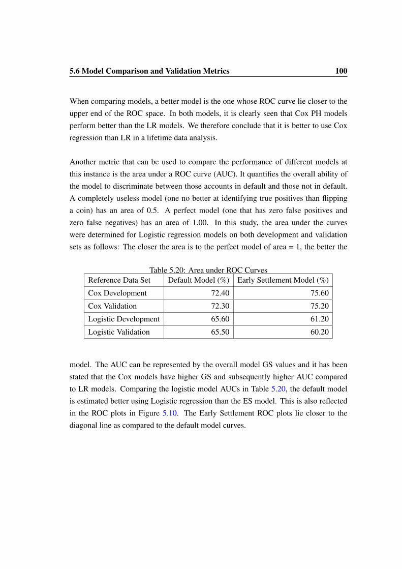
5.6 Model Comparison and Validation Metrics 100
When comparing models, a better model is the one whose ROC curve lie closer to theupper end of the ROC space. In both models, it is clearly seen that Cox PH modelsperform better than the LR models. We therefore conclude that it is better to use Coxregression than LR in a lifetime data analysis.
Another metric that can be used to compare the performance of different models atthis instance is the area under a ROC curve (AUC). It quantifies the overall ability ofthe model to discriminate between those accounts in default and those not in default.A completely useless model (one no better at identifying true positives than flippinga coin) has an area of 0.5. A perfect model (one that has zero false positives andzero false negatives) has an area of 1.00. In this study, the area under the curveswere determined for Logistic regression models on both development and validationsets as follows: The closer the area is to the perfect model of area = 1, the better the
Table 5.20: Area under ROC CurvesReference Data Set Default Model (%) Early Settlement Model (%)
Cox Development 72.40 75.60
Cox Validation 72.30 75.20
Logistic Development 65.60 61.20
Logistic Validation 65.50 60.20
model. The AUC can be represented by the overall model GS values and it has beenstated that the Cox models have higher GS and subsequently higher AUC comparedto LR models. Comparing the logistic model AUCs in Table 5.20, the default modelis estimated better using Logistic regression than the ES model. This is also reflectedin the ROC plots in Figure 5.10. The Early Settlement ROC plots lie closer to thediagonal line as compared to the default model curves.

5.7 Credit Risk Model Standards 101
5.7 Credit Risk Model Standards
The model standards include:
• Minimum data history should be generally at least five years. Models in thisstudy were built based on the observation period covering 5 years (April 2009 toMarch 2014). Every account was tracked on a monthly basis from the point ofentry to exit.
• The data used in the model is representative of the population to be graded. Allavailable data were used.
• A consistent definition of default. The definition of default was consistentlyapplied across the observation period, the same was applied to the definition ofearly settlement.
• Use of the relevant information and data sources. The data used in this study wasobtained from a credible data warehouse which is fully controlled and governedby international standards. All the data extracted relates to the vehicle financeproduct.
• Model drivers that are intuitive and plausible. Model specific covariates wereselected satisfactorily. Evidence is presented, both graphically and numerically.
• Models should meaningfully differentiate risk. Overall model GS for each modelwas determined. The higher the model GS the more capable it is to differentiaterisk.
• Models should be predictive and accurate. An assessment of the actual and pre-dicted observations was conducted. No discrepancies were observed.
• Model outputs that are intuitive and plausible. As in the model drivers, modelspecific output is satisfactory statistically and it makes sound business sense.Results are provided both graphically and numerically.
5.8 Summary 102
5.8 Summary
The model building standards were satisfactorily addressed in each model. Models anddrivers were intuitive and plausible as detailed under each model discussion whereinintuitiveness complements sound business logic. All models have high GS implyingthat they are capable of differentiating risk. Models predictive and accurate metricswere satisfactory. An assessment of the actual and predicted observations was con-ducted. Model GS and ROC curves were calculated to determine the methodologystriving to perform better for a consumer credit cohort data in the presence of com-peting risks and long term survivors. It was concluded that Cox regression performsbetter than Logistic regression.

Chapter 6
Summary, Conclusion andRecommendations
6.1 Introduction
The aims and objectives of this study were to analyse competing risks in a consumercredit context with two events of interest, default and early settlement. These eventswere to be modelled using statistically sound techniques. The bulk of accounts underinvestigation were not susceptible to the events of interest. The data typically had longterm survivors with heavy censoring at the end of the observation period. Two method-ologies were compared in order to establish which works better, given a complex lon-gitudinal cohort data set in the presence of competing risks and long term survivors.The two methodologies are Logistic regression and Cox regression. Model buildingstandards in the credit risk environment were followed to ensure that the models de-veloped were plausible and accurate. Models were developed and methodologies werecompared using the model Gini statistics, receiver operating characteristic curves andarea under the curves. Model output complements theoretical aspects detailed in Chap-ter 2. The data structure is analogous to lifetime data in other domains of study suchas engineering and biomedical research, making the statistical methodologies versatile.

6.2 Summary 104
6.2 Summary
All available vehicle finance data were extracted from the financial institution’s datawarehouse. Data credibility is guaranteed as the data is governed and monitored ac-cording to the internal, national and international standards. Data preparation includedselection of retail accounts opened and recorded in the period April 2009 to March2014, outcome period analysis and derivation of critical variables such as the defaultand early settlement flags. In addition, all available variables were extracted and con-sidered potential covariates unless proven otherwise by statistical and logical argu-ments, all of which were detailed in Chapter 4.
The simple random sampling approach was used to determine the development andhold out independent validation sets in the ratio of 80:20 respectively for each method-ology. For Logistic regression, accounts were allowed 48 months to perform and thebinary target variable was fully observable whereas in Cox regression, the period tomaturity was not considered. Accounts with partially known survival times were in-cluded in the modelling as censored observations. This allowed the use of more infor-mation in Cox regression and less information for Logistic modelling. The volumesused in each method and data set are provided in Table 4.3.
A complete list of covariates was established. Variables with missing values greaterthan 15% were excluded as well as variables which were not consistently populatedback in time. Variables populated with the same value across all observations were ex-cluded as well as categorical covariates which had the number of categories exceeding150. Univariate analysis thoroughly checked the remaining set of potential covariates,each for proportional hazards assumption, population stability, weight of evidence andability to rank order and differentiate risk.
The univariate analysis results are available in Appendix A. Each covariate was ad-vanced to the multivariate analysis process once it had satisfied the univariate analysisconditions. A multivariate analysis was conducted per model per method. The co-variates which satisfied the variance inflation factor analysis, correlation analysis andstatistical significance through stepwise regression were used in the modelling process.

6.3 Conclusion 105
All these were event and method specific.
Logistic regression models were built for each event type. Models were each tested foraccuracy and ability to rank order and differentiate risk. The results were satisfactory.Logistic default and early settlement models were then compared in terms of perfor-mance. Table 5.20 shows a comparison of Logistic models in terms of area under thecurves. It was noted that the Logistic regression methodology was better in predictingdefault than early settlement as the areas under the default model curves are higher thanearly settlement area under the curves. This is also reflected in the receiver operatingcharacteristic curves where early settlement plots lie closer to the diagonal comparedto default curves for the Logistic regression method.
Cause specific Cox regression models were built for each event type and the corre-sponding marginal cumulative probabilities were determined using the CIC. The codeto calculate the CIC was created as it is not present in any of the commercially avail-able statistical applications such as SAS, SPSS and STATA. Models were adjusted toaccommodate long term survivors. The performance of the models was compared us-ing overall model Gini statistics and receiver operating characteristic curves. ClearlyCox regression outperforms Logistic regression as evidenced by higher Gini statisticsand better receiver operating characteristic curves in both default and early settlementmodels. This project was typeset in LATEX and the analysis was conducted in SAS R©.
6.3 Conclusion
Both LR and Cox PH models were developed based on statistically sound techniques,supported by literature. In all models, there is strong empirical support for the resultsas evidenced by the actual versus predicted analyses. All models satisfied conditionslaid out as the Models Building Standards by the internal processes of the financial in-stitution involved. The models managed to predict and correctly classify events in thevalidation set. The models can be used to determine and compare survival prognosisof different risk groups in a consumer credit context. However, LR uses older vintages

6.4 Recommendations 106
in model building, therefore it becomes more difficult to capture the most recent activ-ities. The dependant variable in LR is binary and does not consider time.
The use of survival methods to model credit risk data is motivated by the existence oflifetime loans which can be observed from the point of origin to an event of interest.Survival methods thus, estimate not only if, as in Logistic regression, but also whenborrowers will default. This enhances flexibility as the model generates probabilities ofeach event happening at various points in time. For any given observation period, somecustomers default and some pay-off earlier than the originally agreed term. Where theevent occurs before the end of the observation period, the lifetime of such credits areobservable. For customers who do not default or pay-off early, before the end of theobservation period, it is not possible to observe the time instant when the event occurs.This causes a lack of information due to right censoring.
Censoring allows the response variable to be incompletely determined for some ac-counts. Unlike in the conventional statistical methodologies, censored accounts arenot discarded in survival analysis but contributes information to the study. Censor-ing is the defining feature of survival analysis, making it distinct from other kinds ofanalysis. Logistic regression particularly tends to miss censoring information. Theresponse variable is binary and it should be fully observable. Although in terms of pre-dictive performances the models are substantially similar, survival analysis gives morevaluable information such as a whole predicted survival function rather than a singlepredicted survival probability. Survival analysis is superior to Logistic regression inthat, a better credit granting decision is made if supported by the estimated survivaltimes.
6.4 Recommendations
At a global level, conclusions drawn from the two methods used in this study are essen-tially the same. For the default model, Tables 5.5 and 5.14 provide conclusions drawnfrom Logistic and Cox regression respectively. The same logical trend was reachedimplying that the methodologies complement each other at a global level. This is fur-ther supported by the early settlement models. Tables 5.9 and 5.18 detail Logistic and

6.4 Recommendations 107
Cox regression summaries of the early settlement models respectively showing that theoverall conclusion is the same, regardless of the methodology. It is therefore recom-mend that, if an assessment at a high level is desired, either of the two methodologiescan be utilised, depending on the resources available and simplicity of the methodol-ogy selected.
The outcome or workout period is product and event specific. In this project, the de-tails of the outcome period are provided in Section 4.4.2 where the product is vehiclefinance and events are default and early settlement. It takes 48 months for the bulk ofthe accounts to be absorbed into the events of interest. This outcome period is thenused as the fixed time horizon for which the probabilities are determined. It is interest-ing to see the shift in model performance if the product changes or events are definedsuch that the outcome period is shortened to 24, 12 or 6 months. It is recommend toconduct further analysis with varying products, event types and outcome periods.
The occurrence of early settlement and default events impact negatively on profitabil-ity as part of the anticipated interest (income) will not be realised. Even though bothevents are not good for business, early settlement is a better event than default. Thelender is likely to suffer more in the case of default than in early settlement as there isa possibility of losing a fraction of capital in addition to the interest amount whereas inearly settlement, the lender cannot lose more than the original capital amount issued.There are also penalties charged against the borrower for settling an account early leav-ing the lender in a better position as compared to further losses which may be incurredby the lender in case of default due to follow up and legal costs. It is recommendedthat the financial institution be lenient and waiver some charges against the customerssettling early so that they can retain them in their customer base for future deals.
There are various reasons for customers to settle early. These include switching toanother lender, upgrade to newly released models or settlement due to legal and in-surance claims. With reference to the Type 3 tests in Table 5.16, the main driver ofearly settlement in this model is Equipment Category Code. This classifies new, oldand used vehicles. The old vehicles category entails vehicles older than 5 years at thepoint of application. This category has the highest rate of early settlement. Customers

6.4 Recommendations 108
purchasing old vehicles have a higher chance of settling accounts early as they up-grade to new models. Our recommendation to the financial institution involved in thisstudy is to cap the age of pre-owned vehicles to at most 5 years at the point of purchase.
An analysis was conducted to identify the highest combination of categories with earlysettlement hazard ratio greater than the baseline. These are the customers where thehazards of early settlement happening is greater than those accounts in the baselineand they conversely have a lesser survival prognosis than the customers in the refer-ence group. These customers are living with parents, purchased old vehicles with lowerdebit interest rate and shorter tenure. This conforms to the results explained in Table5.18. If a customer is still living with parents it implies that they are younger, energetic,with minimal responsibilities and would still want to start new deals to purchase newvehicles in future. It is recommended that the financial institution to be more lenientin dealing with this group of customers in order to retain and improve market share inthe future.
As discussed earlier, the default event is worse than the early settlement event. Table5.12 shows Type 3 tests of the default model. The main driver of the default event isDebit Interest Rate. Debit Interest rate is usually calculated based on the risk profile ofthe customer at point of application. If the risk profile tends to high risk, the customeris penalised and allocated a higher interest rate. In practice, debit interest rate is alsoassociated with type of vehicles. The lenders consider the make and model of cars. Forhigh risk vehicles, the debit interest rate is higher. To reach a trade-off between prof-itability and minimising losses due to default, high risk customers may be advised notto purchase vehicles classified as high risk. By so doing the lender avoids penalisingthe customer twice and therefore prevents default and optimises on debit interest.

References
Banasik, J. Crook, J.N. and Thomas, L.C. (1999). Not if but When will BorrowersDefault. The Journal of Operational Research Society. Vol. 50, No. 12, pp.1185-1190.
Basel Committee on Banking Supervision (2006). International Convergence of Cap-
ital Measurement and Capital Standards. Bank for International Settlements,347 pages.
Bellotti, T. and Crook J. (2007). Credit Scoring with Macroeconomic Variables usingSurvival Analysis. International Journal of Bank Marketing. Vol. 54, pp. 276-278.
Cai, Z. and Wheale, P. (2009). Managing Efficient Capital Allocation with Emphasison the Chinese Experience. Journal of Business Ethics. Vol. 87, pp. 111-135.
Capon, N. (1982). Credit Scoring Systems: A critical Analysis. Journal of Marketing.Vol. 46, pp. 82-91.
Cox, D.R. (1972). Regression Model and Life-Tables. Journal of the Royal Statistical
Society. Vol. 34, Series B. pp. 187-220.
Cox, D.R. and Snell, E.J. (1968). A General Definition of Residuals. Journal of the
Royal Statistical Society. Vol. 30, Series B. No. 2, pp. 248-275.
Farewell, V.T (1982). The use of Mixture Models for the Analysis of survival Datawith Long-Term Survivors. Biometrics. Vol. 38, No. 4, pp. 1041-1046.
6.4 Recommendations 110
Fine, J.P. and Gray, R.J. (1999). A Proportional Hazards Model for the Subdistribu-tion of a Competing Risk. Journal of American Statistical Association. Vol. 94,pp. 496-509.
Gini, C. (1936). On the Measure of Concentration with Special Reference to Incomeand Statistics. Colorado College Publication. General Series, No. 208, pp.73-79.
Hand, D.J. and Henley, W.E. (1997). Statistical Classification Methods in ConsumerCredit Scoring: A Review. Journal of the Royal Statistical Society. Vol. 160,Series B. No. 3, pp. 523-541.
Hertz-Picciotto, I. and Rockhill, B. (1997). Validity and Efficiency of ApproximationMethods for Tied Survival Times in Cox Regression. Biometrics. Vol. 53, No.3, pp. 1151-1156.
Hubber, M. and Patetta, M. (2013). Survival Analysis Using the Proportional Hazards
Model Course Notes. 1st ed. SAS R© Institute Inc, 72 pages.
Jilek, O. (2008). Mathematical Applications in Credit Risk Modelling. Journal of
Applied Mathematics. Vol. 1, No. 1, pp. 432-438.
Kleinbaum, D.G. and Klein, M. (2005). Statistics for Biology and Health, Survival
Analysis: A Self Learning Text, 2nd ed., New York: Springer-Verlag Publishers,590 pages.
Le Roux, N.J. and Gardner S. (2005). Analysing Your Multivariate Data as a Pictorial:A Case for Applying Biplot Methodology? International Statistical Review /
Revue Internationale de Statistique. Vol. 73, No. 3, pp. 365-387
Lottes, I.L., DeMaris, A. and Adler, M.A. (1996). Using and Interpreting LogisticRegression: A Guide for Teachers and Students. Teaching Sociology, Vol. 24,No.3, pp. 284-298.
Mansfield, E.R. and Helms, B.P. (1982). Detecting Multicollinearity. The American
Statistician. Vol. 36, No. 3, pp. 158-160.

6.4 Recommendations 111
Migut, G., Jakubowski, J. and Stout, D. (2013). Developing Scorecards Using STA-TISTICA Scorecard. Statsoft Polska/Statsoft Inc.
Odd, O.A., Andersen, P.K., Borgan, O., Gill, R.D. and Keiding, N. (2009). History ofApplications of Martingales in Survival Analysis. Electronic Journal for History
of Probability and Statistics Vol. 5, No. 1, pp. 267-283.
Peng, C.J., Lee, K.L. and Ingersoll, G.M. (2002). An Introduction to Logistic Re-gression Analysis and Reporting. The Journal of Educational Research Vol. 96,No. 1, pp. 3-14.
Schoenfield, D. (1982). Partial Residuals for the Proportional Hazards RegressionModel. Biometrica. Vol. 69, No. 1, pp. 239-241.
Smith, T. and Smith, B. (2000). Survival Analysis And The Application of Cox’sProportional Hazards Modeling. Biometrics. Vol. 54, pp. 244-46.
Stepanova, M. and Thomas L.(2002). Survival Analysis Methods for Personal LoanData. Operations Research. Vol. 50, No. 2, pp. 277-289.
Sy, J.P. and Taylor, J.M.G. (2000). Estimation in a Cox Proportional Hazardsc CureModel. Biometrics. Vol. 56, No. 1, pp. 227-236.
Tableman, M. (2008). Survival Analysis Using S/R, 2nd ed., USA, Chapman andHall/CRC, Chapters 1 to 6, 152 pages.

Appendix A
Univariate Assessment
A.1 Default Model - Initial PH Assessment

A.1 Default Model - Initial PH Assessment 113
Figure A.1: Initial PH Assessment - Default Model

A.2 Default Model - Final PH, Event Rate, Population Stability and WoEAssessment 114
A.2 Default Model - Final PH, Event Rate, Population
Stability and WoE Assessment

A.2 Default Model - Final PH, Event Rate, Population Stability and WoEAssessment 115

A.2 Default Model - Final PH, Event Rate, Population Stability and WoEAssessment 116
Figure A.2: Univariate Assessment - Default Model

A.3 Early Settlement Model - Initial PH Assessment 117
A.3 Early Settlement Model - Initial PH Assessment

A.3 Early Settlement Model - Initial PH Assessment 118
Figure A.3: Initial PH Assessment - ES Model

A.4 ES Model - Final PH, Event Rate, Population Stability and WoE Assessment119
A.4 ES Model - Final PH, Event Rate, Population Sta-
bility and WoE Assessment

A.4 ES Model - Final PH, Event Rate, Population Stability and WoE Assessment120

A.4 ES Model - Final PH, Event Rate, Population Stability and WoE Assessment121
Figure A.4: Univariate Assessment - ES Model

Appendix B
The SAS R© Code
B.1 Data Extraction
PROC SQL;
CREATE TABLE LGD.DATA_ACCOUNT_MONTHLY AS
SELECT * FROM CONNECTION TO ORACLE
( SELECT
SITE_CODE ,
CLOSED_DATE as CLOSED ,
to_number(Account_number) as Account_number,
DATA_COMPANY_CODE as COMPANY_CODE ,
OPEN_DATE as OPEN ,
ACCOUNT_BALANCE ,
ACCUMULATED_INTEREST_AMT ,
OUTSTANDING_CAPITAL_AMT ,
OUTSTANDING_COMMISSION_AMT ,
SUB_PRODUCT_CODE ,
RESIDUAL_VALUE_AMT as RESIDUAL_VALUE ,
YEAR_MODEL ,
CUSTOMER_KEY ,
OUTSTANDING_TERM ,
to_number(to_char(Information_Date,'yyyymm')) as Month,
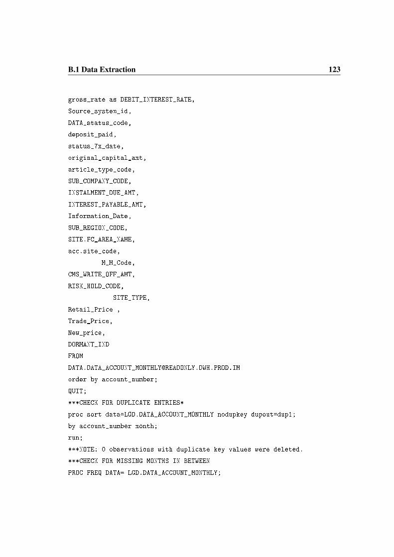
B.1 Data Extraction 123
gross_rate as DEBIT_INTEREST_RATE,
Source_system_id,
DATA_status_code,
deposit_paid,
status_7x_date,
original_capital_amt,
article_type_code,
SUB_COMPANY_CODE,
INSTALMENT_DUE_AMT,
INTEREST_PAYABLE_AMT,
Information_Date,
SUB_REGION_CODE,
SITE.FC_AREA_NAME,
acc.site_code,
M_M_Code,
CMS_WRITE_OFF_AMT,
RISK_HOLD_CODE,
SITE_TYPE,
Retail_Price ,
Trade_Price,
New_price,
DORMANT_IND
FROM
order by account_number;
QUIT;
***CHECK FOR DUPLICATE ENTRIES*
proc sort data=LGD.DATA_ACCOUNT_MONTHLY nodupkey dupout=dup1;
by account_number month;
run;
***NOTE: 0 observations with duplicate key values were deleted.
***CHECK FOR MISSING MONTHS IN BETWEEN
PROC FREQ DATA= LGD.DATA_ACCOUNT_MONTHLY;
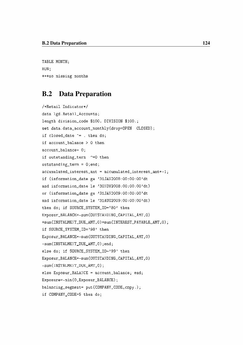
B.2 Data Preparation 124
TABLE MONTH;
RUN;
***no missing months
B.2 Data Preparation
/*Retail Indicator*/
data lgd.Retail_Accounts;
length division_code $100. DIVISION $100.;
set data.data_account_monthly(drop=OPEN CLOSED);
if closed_date ^= . then do;
if account_balance > 0 then
account_balance= 0;
if outstanding_term ^=0 then
outstanding_term = 0;end;
accumulated_interest_amt = accumulated_interest_amt*-1;
if (information_date ge '31JAN2008:00:00:00'dt
and information_date le '30NOV2008:00:00:00'dt)
or (information_date ge '31JAN2009:00:00:00'dt
and information_date le '31AUG2009:00:00:00'dt)
then do; if SOURCE_SYSTEM_ID='80' then
Exposur_BALANCE=-sum(OUTSTANDING_CAPITAL_AMT,0)
+sum(INSTALMENT_DUE_AMT,0)+sum(INTEREST_PAYABLE_AMT,0);
if SOURCE_SYSTEM_ID='99' then
Exposur_BALANCE=-sum(OUTSTANDING_CAPITAL_AMT,0)
-sum(INSTALMENT_DUE_AMT,0);end;
else do; if SOURCE_SYSTEM_ID='99' then
Exposur_BALANCE=-sum(OUTSTANDING_CAPITAL_AMT,0)
-sum(INSTALMENT_DUE_AMT,0);
else Exposur_BALANCE = account_balance; end;
Exposure=-min(0,Exposur_BALANCE);
balancing_segment= put(COMPANY_CODE,cmpy.);
if COMPANY_CODE=5 then do;

B.2 Data Preparation 125
DIVISION_CODE='5';
if SUB_COMPANY_CODE=4 then
SUB_DIVISION_CODE='FCR';
else if SUB_COMPANY_CODE=5 then
SUB_DIVISION_CODE='MAF';
else if SUB_COMPANY_CODE=19 then
SUB_DIVISION_CODE='VCF';
else if SUB_COMPANY_CODE=23 then
SUB_DIVISION_CODE='LRF';
else if SUB_COMPANY_CODE=35 then
SUB_DIVISION_CODE='JAG';
else if SUB_COMPANY_CODE=42 then
SUB_DIVISION_CODE='42'; end;
else if COMPANY_CODE=39 then do;
DIVISION_CODE='39';
if SITE_CODE=5488 then
SUB_DIVISION_CODE='CRD';
else if SITE_CODE=5552 then
SUB_DIVISION_CODE='EPL';
else SUB_DIVISION_CODE='NWB';
end;
else if COMPANY_CODE>100 then do;
DIVISION_CODE='OTH';
if COMPANY_CODE=144 then
SUB_DIVISION_CODE='PVB';end;
else if
SITE_CODE in ('5352','5351','5596','5498','5307','5571')
then do;
DIVISION_CODE='ENT';
SUB_DIVISION_CODE='ENT';end;
else if
COMPANY_CODE
in (22,28,31,36,37,38,40,41,45,51,52,54,55,70) then do;
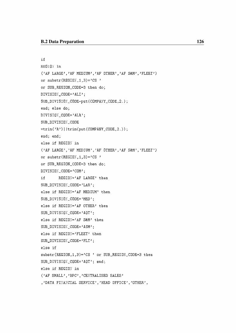
B.2 Data Preparation 126
if
REGION in
('AF LARGE','AF MEDIUM','AF OTHER','AF S&M','FLEET')
or substr(REGION,1,3)='CS '
or SUB_REGION_CODE=3 then do;
DIVISION_CODE='ALI';
SUB_DIVISION_CODE=put(COMPANY_CODE,2.);
end; else do;
DIVISION_CODE='ALR';
SUB_DIVISION_CODE
=trim('R')||trim(put(COMPANY_CODE,2.));
end; end;
else if REGION in
('AF LARGE','AF MEDIUM','AF OTHER','AF S&M','FLEET')
or substr(REGION,1,3)='CS '
or SUB_REGION_CODE=3 then do;
DIVISION_CODE='COM';
if REGION='AF LARGE' then
SUB_DIVISION_CODE='LAR';
else if REGION='AF MEDIUM' then
SUB_DIVISION_CODE='MED';
else if REGION='AF OTHER' then
SUB_DIVISION_CODE='AOT';
else if REGION='AF S&M' then
SUB_DIVISION_CODE='ASM';
else if REGION='FLEET' then
SUB_DIVISION_CODE='FLT';
else if
substr(REGION,1,3)='CS ' or SUB_REGION_CODE=3 then
SUB_DIVISION_CODE='AOT'; end;
else if REGION in
('AF SMALL','BPC','CENTRALISED SALES'
,'DATA FINANCIAL SERVICE','HEAD OFFICE','OTHER',

B.2 Data Preparation 127
'Personal Sales
Dealers','Personal Sales Internal','Personal Sales Small',
'Risk Management','', 'SMALL','SMALL-Dormant' ,'Private Bank')
then do;
DIVISION_CODE='RET';
if REGION in ('AF SMALL','SMALL') then
SUB_DIVISION_CODE='SML';
else if REGION ='BPC' then
SUB_DIVISION_CODE='BPC';
else if
REGION in ('CENTRALISED SALES')
or substr(REGION,1,3)='CS ' then
SUB_DIVISION_CODE='CEN';
else if REGION ='DATA FINANCIAL SERVICE' then
SUB_DIVISION_CODE='DATA';
else if REGION ='HEAD OFFICE' then
SUB_DIVISION_CODE='HOF';
else if REGION ='OTHER' then
SUB_DIVISION_CODE='OTH';
else if REGION ='Personal Sales Dealers' then
SUB_DIVISION_CODE='PSD';
else if REGION ='Personal Sales Internal' then
SUB_DIVISION_CODE='PSI';
else
if REGION in
('Personal Sales Small','SMALL-Dormant') then
SUB_DIVISION_CODE='PSS';
else if REGION ='Risk Management' then
SUB_DIVISION_CODE='RSM';
else if REGION ='Private Bank' then
SUB_DIVISION_CODE='AFL';
else if REGION ='' then
SUB_DIVISION_CODE='UNK'; end; else
B.2 Data Preparation 128
do; put '*** New value found for Region ***';
put SITE_CODE= REGION=;
abort; end;
select (DIVISION_CODE);
when('5') do; DIVISION='Ford Credit'; ORDERING=5; end;
when('15')do; DIVISION='Unitrans'; ORDERING=8; end;
when('21')do; DIVISION='MEEG'; ORDERING=7; end;
when('39')do; DIVISION='MAN'; ORDERING=4; end;
when('SEC')
do;DIVISION='Securitisation';ORDERING=6;end;
when('OTH')do;DIVISION='Other';ORDERING=14;end;
when('ALI')do;DIVISION='Alliances';ORDERING=15; end;
when('ALR')do;
DIVISION='Alliances Retail';ORDERING=13;end;
when('COM')do;DIVISION='Commercial';
ORDERING=2;end;
when('COR')do;DIVISION='Corporate';ORDERING=1;end;
when('RET') do;DIVISION='Retail';ORDERING=3;end;
when('ENT')do;DIVISION='Enterprise';ORDERING=9; end;
otherwise;end;
if balancing_segment ^= 'SEC'
then gl_division=balancing_segment;
else if COMPANY_CODE = 58 thenR
gl_division='CAR2';
else if COMPANY_CODE = 95 then gl_division='CAR1';
else gl_division='SEC'; if (balancing_segment in ('DATA')
and compress(division) in ('','Retail')
or balancing_segment in ('DATA')
and compress(DIVISION_CODE) in ('','ALR')
Or balancing_segment in ('SEC')
and compress(division) in ('','Retail','Securitisation')
Or balancing_segment in ('BOT','DATA','VODA'))
and commercial_ind ^= "YES" then
B.3 Derivation of Critical Fields 129
Retail_Indicator = 1;
B.3 Derivation of Critical Fields
/*Default flag*/
Data LGD.DEFAULT_ACCOUNTS
(rename =
(DATA_status_code =
DATA_sc_org DATA_status_code1 = DATA_status_code));
set LGD.RETAIL_ACCOUNTS;
if source_system_id = '80' then do;
if status_7x_date ne . then
DATA_status_code1 = 70;
else DATA_status_code1 = DATA_status_code;
if arrear_payments_due_count >= 3 then
DATA_status_code1 = 40; end;
if source_system_id = '99' then do;
if risk_hold_code = 'FWO' then
DATA_status_code1 = 70;
else if site_type in ('071','087') then
DATA_status_code1 = 69;
else if arrear_payments_due_count >= 7 then
DATA_status_code1 = 40;
else DATA_status_code1 = 10; end;
run;
data LGD.BASEDATA;
set LGD.DEFAULT_ACCOUNTS;
if (DATA_status_code >= 40 and DATA_status_code <= 79)
then default = 1; else default = 0; run;
data workingfile;
B.3 Derivation of Critical Fields 130
set LGD.BASEDATA;
by account_number;
if first.account_number then do;
if close ne . and exposure = 0
and interest_payable_amt = 0
and instalment_due_amt = 0
and residual_value_amt = 0
and close = month
and outstanding_term = 0
then do; closed_ind = 1;
closed_month = close;end;
else do; closed_ind = 0; closed_month = .; end; end;
retain closed_ind closed_month;
lifetime = -1*((-1*intck('month',input(put(open,best6.)
,yymmn6.) ,input(put(closed_month,best6.),yymmn6.)))); run;
proc sort
data=workingfile; by account_number descending month ; run;
data sa.accountage;
set workingfile;
age_of_account =
-1*((-1*intck('month',input(put(open,best6.),yymmn6.)
,input(put(month,best6.),yymmn6.))));
by account_number;
if first.account_number
do;
if closed_ind = 1 and
default ne 1 and lifetime lt original_term then do;
es = 1; es_month = closed_month;
end; else do; es = 0; es_month = .; end; end;
retain es es_month;
***Censoring
proc sort data=LGD.BASEDATA; by account_number descending month;run;

B.4 Covariate Selection 131
data sa.censored;
set LGD.BASEDATA;
by account_number;
if first.account_number then do;
if default ne 1 and es ne 1 then do; censor = 1;
censor_month = month; end;else do;
censor = 0;
censor_month = .; end; end;
retain censor censor_month;
if def_month ne . then
event_month = def_month;
else if es_month ne . then
event_month = es_month;
else event_month = censor_month;
survtime=-1*((-1*intck('month',input(put(open,best6.),yymmn6.)
,input(put(event_month,best6.),yymmn6.))));
run;
B.4 Covariate Selection
PROC SQL;
CREATE TABLE SA.STATS_ACCOUNT_MONTHLY AS
SELECT * FROM CONNECTION TO ORACLE
(SELECT
to_number(Account_number) as Account_number ,
to_number(to_char(Information_Date,'yyyymm')) as Month,
RESIDUAL_VALUE_AMT,
ADDITIONAL_CAPITAL_AMT,
OPEN_DATE,
DATA_COMPANY_CODE,
DEPOSIT_PAID,
EXTRAS_FINANCED_AMT,
INSTALMENT_FREQUENCY_CODE,

B.4 Covariate Selection 132
ORIGINAL_BALANCE,
ORIGINAL_CAPITAL_AMT,
ORIGINAL_INSTALMENT_AMT,
ORIGINAL_INTEREST_AMT,
ORIGINAL_PRIME_RATE,
ORIGINAL_TERM,
YEAR_MODEL,
ACCOUNT_TYPE_CODE,
ARTICLE_TYPE_CODE,
ASSET_LIABILITY_IND,
DATA_STATUS_CODE,
DATA_INSTALMENT_METHOD_CODE,
DATA_RATE_TYPE_CODE,
CREDIT_AGREEMENT_LAW_IND,
DISCOUNTING_CODE,
EQUIPMENT_CATEGORY_CODE,
NEW_OLD_USED,
RE_CREATION_IND,
ACCOUNT_SECURITY,
ARTICLE_TYPE_CODE,
DATE_OF_BIRTH,
DEPOSIT_PAID,
DWELLING_TYPE_CODE,
EXTRAS_FINANCED_AMT,
INSTALMENT_FREQUENCY_CODE,
MAINTENANCE_CODE,
MANUFACTURER_CODE,
MARITAL_STATUS_CODE,
NET_INCOME,
NUMBER_OF_DEPENDANTS,
NUMBER_OF_INQUIRIES,
NUMBER_OF_INSURANCES,
OCCUPATION_CODE,

B.4 Covariate Selection 133
PRODUCT_CODE,
RESIDUAL_VALUE,
SA_CITIZEN_IND,
SPOUSE_EMPLOYED_IND,
SPOUSE_INCOME_AMT,
TIME_AT_CURRENT_ADDRESS,
TIME_IN_CURRENT_JOB,
TOTAL_DEFAULTS_EVER_10,
TOTAL_LIVING_EXPENSES
FROM [email protected] )
where
account_number in
(select account_number from SA.BASEDATA4)
order by account_number;
DISCONNECT FROM ORACLE; QUIT;
proc sql;
create table sa.basedata5 as
select a. *,
b. *,
c. *
from (select * from sa.base5 as a
left join STATS_ACCOUNT_MONTHLY as b
on a. account_number = b. account_number
left join STATIC_MANUFACTURER_MONTHLY as c
on a. M_M_Code = c. M_M_Code and a. month = c. month;
quit;
*** Derived Covariates
DATA sa.basedata5;
SET sa.basedata5;
model_month = year_model * 100 + 1;
Age_of_asset
= (-1*((-1*intck('month',input(put(model_month,$6.),yymmn6.)
,input(put(month,$6.),yymmn6.)))))/12;

B.4 Covariate Selection 134
Application_IIR = ORIGINAL_INSTALMENT_AMT/CUSTOMER_INCOME_AMT;
Current_IIR = INSTALMENT_DUE_AMT/CUSTOMER_INCOME_AMT;
Deposit_to_Loan = Deposit_Paid/ORIGINAL_CAPITAL_AMT;
Ballon_to_Loan = RESIDUAL_VALUE_AMT/ORIGINAL_CAPITAL_AMT;
Age_of_Applicant = (-1*((-1*intck('month',input(put(DOB,$6.),
yymmn6.)
,input(put(month,$6.),yymmn6.)))))/12;
LTV = Original_Balance/Trade_Price; run;
***Numerical Variable Selection
proc summary data=sa.base3 nway missing; ar _numeric_;
output out=descriptivestats;quit;
data base3;
set sa.base3;drop
residual_value
information_date
status_7x_date
status_70_loss
number_instalment_in_arrear
cms_write_off_amt
ordering
age_of_account
NUMBER_OF_INQUIRIES
NUMBER_OF_DEPENDANTS
TIME_AT_CURRENT_ADDRESS
Application_IIR
Current_IIR
TOTAL_DEFAULTS_EVER_10
Customer_Income_amt; run;
/*1) count number of missing numeric values for each variable*/
data missing_nums;
set base3; format _numeric_ best8.;
array nums _numeric_;
keep _numeric_;
B.4 Covariate Selection 135
do i = 1 to dim(nums);
if nums[i] = . then
nums[i] = 1;
else nums[i] = 0; end; drop i; run;
proc summary data= missing_nums nway missing;
var _numeric_; output sum= out=missing_nums; quit;
proc transpose data=missing_nums (drop=_type_ _freq_)
out=missing_nums name=variable; run;
***create a
variable for the number of missing values greater than threshold*/
proc sql noprint;
select count(*) into:numvar
from missing_nums;
select count(*) into:devnobs
from lgd.account_monthly_covariates; quit;
data missing_nums (drop=_label_);
set missing_nums;
format concat $10240.;
retain concat '';
pmissing = col1/&devnobs.;
if pmissing > 0.15
and variable not in ("account_number", "month" ,"closed_ind",
"closed_month","default","def_month",
"es", "es_month", "censor", "censor_month",
"event_month", "survtime") then
concat = trim(concat)||' '||compress(variable);
if _n_ = &numvar. then
call symput("numvar",put(trim(concat),$10240.));run;
***Calculate the number of missing levels for each variable
ods output nlevels=levels;
proc freq data=sa.base3 nlevels;
tables _char_/ noprint; run; ods output close;
***Create a variable for the number of variables with number

B.5 Univariate Analysis 136
of levels greater than threshold and where a variable
has a single level*/
proc sql noprint;
select count(*) into:charvar from levels; quit;
data levels; set levels (rename=(tablevar=variable));
format concat $10240.; retain concat '';
plevels = nlevels/&devnobs.;
if nlevels > 150 or nlevels = 1 then
concat = trim(concat)||' '||compress(variable);
if _n_ = &charvar. then
call symput("charvar",put(trim(concat),$10240.)); run;
data base4;
set base3;
drop &numvar. &charvar. run;
B.5 Univariate Analysis
****Sampling
/*Validation set (20%) = 73452 accounts*/
proc surveyselect
data=base4 out=sa.validation method=srs n=73452 seed=20140922; run;
proc sql;
create table sa.development
as select * from base4 where account_number
not in (select account_number from sa.validation); quit;
data manufacturer;
set sa.base3;
manufacturer_code = substr(M_M_Code,1,3); run;
proc sql;
create table development as
select a.*,
b. manufacturer_code
from sa.development as a

B.5 Univariate Analysis 137
left join manufacturer as b
on a. account_number = b. account_number; quit;
data sa.default;
set development;
length _UFormat $200;
drop _UFormat;
_UFormat='';
*------------------------------------------------------------*;
* Variable: ARTICLE_TYPE_CODE;
*------------------------------------------------------------*;
LABEL GRP_ARTICLE_TYPE_CODE = 'Grouped: ARTICLE_TYPE_CODE';
LABEL
WOE_ARTICLE_TYPE_CODE = 'Weight of Evidence: ARTICLE_TYPE_CODE';
_UFormat = put(ARTICLE_TYPE_CODE,$3.0);
%dmnormip(_UFormat);
if MISSING(_UFORMAT) then do;
GRP_ARTICLE_TYPE_CODE = 1;
WOE_ARTICLE_TYPE_CODE = -0.190237734;
end;
else if NOT MISSING(_UFORMAT) then do;
if (_UFORMAT eq 'CRV' OR _UFORMAT
eq 'HOR' OR _UFORMAT eq 'LDV' OR _UFORMAT eq 'MBK'
OR _UFORMAT eq 'MIN' OR _UFORMAT
eq 'TRK' OR _UFORMAT eq 'TRL' OR _UFORMAT eq 'TRS'
) then do;
GRP_ARTICLE_TYPE_CODE = 1;
WOE_ARTICLE_TYPE_CODE = -0.190237734;
end;
else
if (_UFORMAT eq 'BOT' OR _UFORMAT eq 'MVH'
) then do;
GRP_ARTICLE_TYPE_CODE = 2;
WOE_ARTICLE_TYPE_CODE = 0.070567735;
B.5 Univariate Analysis 138
end;
else do;
GRP_ARTICLE_TYPE_CODE = 1;
WOE_ARTICLE_TYPE_CODE = -0.190237734;
end;
end;
*------------------------------------------------------------*;
* Variable: Age_of_asset;
*------------------------------------------------------------*;
LABEL GRP_Age_of_asset = 'Grouped: Age_of_asset';
LABEL WOE_Age_of_asset = 'Weight of Evidence: Age_of_asset';
if MISSING(Age_of_asset) then do;
GRP_Age_of_asset = 3;
WOE_Age_of_asset = -0.138195006;
end;
else if NOT MISSING(Age_of_asset) then do;
if Age_of_asset < 2 then do;
GRP_Age_of_asset = 1;
WOE_Age_of_asset = 0.1158359209;
end;
else
if 2 <= Age_of_asset AND Age_of_asset < 3.67 then do;
GRP_Age_of_asset = 2;
WOE_Age_of_asset = -0.095049539;
end;
else
if 3.67 <= Age_of_asset then do;
GRP_Age_of_asset = 3;
WOE_Age_of_asset = -0.138195006;
end;
end;
*------------------------------------------------------------*;
* Variable: DEBIT_INTEREST_RATE;

B.5 Univariate Analysis 139
*------------------------------------------------------------*;
LABEL GRP_DEBIT_INTEREST_RATE = 'Grouped: DEBIT_INTEREST_RATE';
LABEL WOE_DEBIT_INTEREST_RATE
= 'Weight of Evidence: DEBIT_INTEREST_RATE';
if MISSING(DEBIT_INTEREST_RATE) then do;
GRP_DEBIT_INTEREST_RATE = 3;
WOE_DEBIT_INTEREST_RATE = 0.2476004225;
end;
else if NOT MISSING(DEBIT_INTEREST_RATE) then do;
if DEBIT_INTEREST_RATE < 10 then do;
GRP_DEBIT_INTEREST_RATE = 1;
WOE_DEBIT_INTEREST_RATE = 1.316778244;
end;
else
if 10 <= DEBIT_INTEREST_RATE AND DEBIT_INTEREST_RATE < 11 then do;
GRP_DEBIT_INTEREST_RATE = 2;
WOE_DEBIT_INTEREST_RATE = 0.8624454296;
end;
else
if 11 <= DEBIT_INTEREST_RATE AND
DEBIT_INTEREST_RATE < 12.55 then do;
GRP_DEBIT_INTEREST_RATE = 3;
WOE_DEBIT_INTEREST_RATE = 0.2476004225;
end;
else
if 12.55 <= DEBIT_INTEREST_RATE
AND DEBIT_INTEREST_RATE < 14.2 then do;
GRP_DEBIT_INTEREST_RATE = 4;
WOE_DEBIT_INTEREST_RATE = -0.298184443;
end;
else
if 14.2 <= DEBIT_INTEREST_RATE then do;
GRP_DEBIT_INTEREST_RATE = 5;

B.5 Univariate Analysis 140
WOE_DEBIT_INTEREST_RATE = -0.814975572;
end;
end;
*------------------------------------------------------------*;
* Variable: DEPOSIT_PAID;
*------------------------------------------------------------*;
LABEL GRP_DEPOSIT_PAID = 'Grouped: DEPOSIT_PAID';
LABEL WOE_DEPOSIT_PAID = 'Weight of Evidence: DEPOSIT_PAID';
if MISSING(DEPOSIT_PAID) then do;
GRP_DEPOSIT_PAID = 1;
WOE_DEPOSIT_PAID = 0.064037842;
end;
else if NOT MISSING(DEPOSIT_PAID) then do;
if 0 <= DEPOSIT_PAID AND DEPOSIT_PAID < 9000 then do;
GRP_DEPOSIT_PAID = 1;
WOE_DEPOSIT_PAID = 0.064037842;
end;
else
if 9000 <= DEPOSIT_PAID AND DEPOSIT_PAID < 20000 then do;
GRP_DEPOSIT_PAID = 2;
WOE_DEPOSIT_PAID = -0.337951621;
end;
else
if 20000 <= DEPOSIT_PAID AND DEPOSIT_PAID < 30000 then do;
GRP_DEPOSIT_PAID = 3;
WOE_DEPOSIT_PAID = -0.189797344;
end;
else
if 30000 <= DEPOSIT_PAID AND DEPOSIT_PAID < 68000 then do;
GRP_DEPOSIT_PAID = 4;
WOE_DEPOSIT_PAID = -0.015375292;
end;
else

B.5 Univariate Analysis 141
if 68000 <= DEPOSIT_PAID then do;
GRP_DEPOSIT_PAID = 5;
WOE_DEPOSIT_PAID = 0.5235175903;
end;
end;
*------------------------------------------------------------*;
* Variable: Deposit_to_Loan;
*------------------------------------------------------------*;
LABEL GRP_Deposit_to_Loan = 'Grouped: Deposit_to_Loan';
LABEL WOE_Deposit_to_Loan = 'Weight of Evidence: Deposit_to_Loan';
if MISSING(Deposit_to_Loan) then do;
GRP_Deposit_to_Loan = 3;
WOE_Deposit_to_Loan = 0.4668041512;
end;
else if NOT MISSING(Deposit_to_Loan) then do;
if Deposit_to_Loan < 0.34 then do;
GRP_Deposit_to_Loan = 1;
WOE_Deposit_to_Loan = -0.045864396;
end;
else
if 0.34 <= Deposit_to_Loan AND Deposit_to_Loan < 0.45 then do;
GRP_Deposit_to_Loan = 2;
WOE_Deposit_to_Loan = 0.0348316203;
end;
else
if 0.45 <= Deposit_to_Loan then do;
GRP_Deposit_to_Loan = 3;
WOE_Deposit_to_Loan = 0.4668041512;
end;
end;
*------------------------------------------------------------*;
* Variable: Exposure;
*------------------------------------------------------------*;

B.5 Univariate Analysis 142
LABEL GRP_Exposure = 'Grouped: Exposure';
LABEL WOE_Exposure = 'Weight of Evidence: Exposure';
if MISSING(Exposure) then do;
GRP_Exposure = 4;
WOE_Exposure = 0.1346572287;
end;
else if NOT MISSING(Exposure) then do;
if Exposure < 98140.01 then do;
GRP_Exposure = 1;
WOE_Exposure = -0.229444959;
end;
else
if 98140.01 <= Exposure AND Exposure < 133558.66 then do;
GRP_Exposure = 2;
WOE_Exposure = -0.079484352;
end;
else
if 133558.66 <= Exposure AND Exposure < 152482.08 then do;
GRP_Exposure = 3;
WOE_Exposure = 0.0358432893;
end;
else
if 152482.08 <= Exposure then do;
GRP_Exposure = 4;
WOE_Exposure = 0.1346572287;
end;
end;
*------------------------------------------------------------*;
* Variable: MARITAL_STATUS_CODE;
*------------------------------------------------------------*;
LABEL GRP_MARITAL_STATUS_CODE = 'Grouped: MARITAL_STATUS_CODE';
LABEL WOE_MARITAL_STATUS_CODE =
'Weight of Evidence: MARITAL_STATUS_CODE';

B.5 Univariate Analysis 143
if MISSING(MARITAL_STATUS_CODE) then do;
GRP_MARITAL_STATUS_CODE = 1;
WOE_MARITAL_STATUS_CODE = -0.119971765;
end;
else if NOT MISSING(MARITAL_STATUS_CODE) then do;
if 1 <= MARITAL_STATUS_CODE AND MARITAL_STATUS_CODE < 3 then do;
GRP_MARITAL_STATUS_CODE = 1;
WOE_MARITAL_STATUS_CODE = -0.119971765;
end;
else
if 3 <= MARITAL_STATUS_CODE then do;
GRP_MARITAL_STATUS_CODE = 2;
WOE_MARITAL_STATUS_CODE = 0.1269054955;
end;
end;
*------------------------------------------------------------*;
* Variable: NUMBER_OF_INSURANCES;
*------------------------------------------------------------*;
LABEL GRP_NUMBER_OF_INSURANCES = 'Grouped: NUMBER_OF_INSURANCES';
LABEL WOE_NUMBER_OF_INSURANCES =
'Weight of Evidence: NUMBER_OF_INSURANCES';
if MISSING(NUMBER_OF_INSURANCES) then do;
GRP_NUMBER_OF_INSURANCES = 2;
WOE_NUMBER_OF_INSURANCES = -0.27230291;
end;
else if NOT MISSING(NUMBER_OF_INSURANCES) then do;
if 0 <= NUMBER_OF_INSURANCES AND NUMBER_OF_INSURANCES < 3 then do;
GRP_NUMBER_OF_INSURANCES = 1;
WOE_NUMBER_OF_INSURANCES = 0.0222955252;
end;
else
if 3 <= NUMBER_OF_INSURANCES then do;
GRP_NUMBER_OF_INSURANCES = 2;

B.5 Univariate Analysis 144
WOE_NUMBER_OF_INSURANCES = -0.27230291;
end;
end;
*------------------------------------------------------------*;
* Variable: ORIGINAL_BALANCE;
*------------------------------------------------------------*;
LABEL GRP_ORIGINAL_BALANCE = 'Grouped: ORIGINAL_BALANCE';
LABEL WOE_ORIGINAL_BALANCE = 'Weight of Evidence: ORIGINAL_BALANCE';
if MISSING(ORIGINAL_BALANCE) then do;
GRP_ORIGINAL_BALANCE = 2;
WOE_ORIGINAL_BALANCE = -0.052907499;
end;
else if NOT MISSING(ORIGINAL_BALANCE) then do;
if ORIGINAL_BALANCE < 122358.98 then do;
GRP_ORIGINAL_BALANCE = 1;
WOE_ORIGINAL_BALANCE = -0.171879447;
end;
else
if 122358.98
<= ORIGINAL_BALANCE AND ORIGINAL_BALANCE < 247063.33 then do;
GRP_ORIGINAL_BALANCE = 2;
WOE_ORIGINAL_BALANCE = -0.052907499;
end;
else
if 247063.33 <=
ORIGINAL_BALANCE AND ORIGINAL_BALANCE < 293882.74 then do;
GRP_ORIGINAL_BALANCE = 3;
WOE_ORIGINAL_BALANCE = 0.0708255812;
end;
else
if 293882.74 <=
ORIGINAL_BALANCE AND ORIGINAL_BALANCE < 575945.07 then do;
GRP_ORIGINAL_BALANCE = 4;
B.5 Univariate Analysis 145
WOE_ORIGINAL_BALANCE = 0.2070221793;
end;
else
if 575945.07 <= ORIGINAL_BALANCE then do;
GRP_ORIGINAL_BALANCE = 5;
WOE_ORIGINAL_BALANCE = -0.041999079;
end;
end;
*------------------------------------------------------------*;
* Variable: ORIGINAL_TERM;
*------------------------------------------------------------*;
LABEL GRP_ORIGINAL_TERM = 'Grouped: ORIGINAL_TERM';
LABEL WOE_ORIGINAL_TERM = 'Weight of Evidence: ORIGINAL_TERM';
if MISSING(ORIGINAL_TERM) then do;
GRP_ORIGINAL_TERM = 4;
WOE_ORIGINAL_TERM = 0.113416106;
end;
else if NOT MISSING(ORIGINAL_TERM) then do;
if 48 <= ORIGINAL_TERM AND ORIGINAL_TERM < 54 then do;
GRP_ORIGINAL_TERM = 1;
WOE_ORIGINAL_TERM = -0.477796284;
end;
else
if 54 <= ORIGINAL_TERM AND ORIGINAL_TERM < 60 then do;
GRP_ORIGINAL_TERM = 2;
WOE_ORIGINAL_TERM = -0.104678453;
end;
else
if 60 <= ORIGINAL_TERM AND ORIGINAL_TERM < 72 then do;
GRP_ORIGINAL_TERM = 3;
WOE_ORIGINAL_TERM = -0.033932584;
end;
else
B.5 Univariate Analysis 146
if 72 <= ORIGINAL_TERM then do;
GRP_ORIGINAL_TERM = 4;
WOE_ORIGINAL_TERM = 0.113416106;
end;
end;
*------------------------------------------------------------*;
* Variable: DATA_RATE_TYPE_CODE;
*------------------------------------------------------------*;
LABEL GRP_DATA_RATE_TYPE_CODE = 'Grouped: DATA_RATE_TYPE_CODE';
LABEL WOE_DATA_RATE_TYPE_CODE =
'Weight of Evidence: DATA_RATE_TYPE_CODE';
_UFormat = put(DATA_RATE_TYPE_CODE,$1.0);
%dmnormip(_UFormat);
if MISSING(_UFORMAT) then do;
GRP_DATA_RATE_TYPE_CODE = 2;
WOE_DATA_RATE_TYPE_CODE = -0.078813438;
end;
else if NOT MISSING(_UFORMAT) then do;
if (_UFORMAT eq 'B' OR _UFORMAT eq 'G'
) then do;
GRP_DATA_RATE_TYPE_CODE = 1;
WOE_DATA_RATE_TYPE_CODE = 0.3833158125;
end;
else
if (_UFORMAT eq 'O'
) then do;
GRP_DATA_RATE_TYPE_CODE = 2;
WOE_DATA_RATE_TYPE_CODE = -0.078813438;
end;
else do;
GRP_DATA_RATE_TYPE_CODE = 2;
WOE_DATA_RATE_TYPE_CODE = -0.078813438;
end;

B.5 Univariate Analysis 147
end;
*------------------------------------------------------------*;
* Variable: DWELLING_TYPE_CODE;
*------------------------------------------------------------*;
LABEL GRP_DWELLING_TYPE_CODE = 'Grouped: DWELLING_TYPE_CODE';
LABEL WOE_DWELLING_TYPE_CODE =
'Weight of Evidence: DWELLING_TYPE_CODE';
_UFormat = put(DWELLING_TYPE_CODE,$1.0);
%dmnormip(_UFormat);
if MISSING(_UFORMAT) then do;
GRP_DWELLING_TYPE_CODE = 3;
WOE_DWELLING_TYPE_CODE = 0.2198800801;
end;
else if NOT MISSING(_UFORMAT) then do;
if (_UFORMAT eq 'T'
) then do;
GRP_DWELLING_TYPE_CODE = 1;
WOE_DWELLING_TYPE_CODE = -0.236749091;
end;
else
if (_UFORMAT eq 'B' OR _UFORMAT eq 'P'
) then do;
GRP_DWELLING_TYPE_CODE = 2;
WOE_DWELLING_TYPE_CODE = -0.04388855;
end;
else
if (_UFORMAT eq 'O'
) then do;
GRP_DWELLING_TYPE_CODE = 3;
WOE_DWELLING_TYPE_CODE = 0.2198800801;
end;
else do;
GRP_DWELLING_TYPE_CODE = 3;

B.5 Univariate Analysis 148
WOE_DWELLING_TYPE_CODE = 0.2198800801;
end;
end;
*------------------------------------------------------------*;
* Variable: EQUIPMENT_CATEGORY_CODE;
*------------------------------------------------------------*;
LABEL GRP_EQUIPMENT_CATEGORY_CODE =
'Grouped: EQUIPMENT_CATEGORY_CODE';
LABEL WOE_EQUIPMENT_CATEGORY_CODE =
'Weight of Evidence: EQUIPMENT_CATEGORY_CODE';
_UFormat = put(EQUIPMENT_CATEGORY_CODE,$6.0);
%dmnormip(_UFormat);
if MISSING(_UFORMAT) then do;
GRP_EQUIPMENT_CATEGORY_CODE = 3;
WOE_EQUIPMENT_CATEGORY_CODE = -0.071746202;
end;
else if NOT MISSING(_UFORMAT) then do;
if (_UFORMAT eq 'AGRICU'
OR _UFORMAT eq 'CARAVN' OR _UFORMAT eq 'LDV<5Y'
OR _UFORMAT eq 'OTHER') then do;
GRP_EQUIPMENT_CATEGORY_CODE = 1;
WOE_EQUIPMENT_CATEGORY_CODE = -0.29965709;
end;
else
if (_UFORMAT eq 'LDVNEW' OR _UFORMAT eq 'MTBIKE'
) then do;
GRP_EQUIPMENT_CATEGORY_CODE = 2;
WOE_EQUIPMENT_CATEGORY_CODE = -0.099150242;
end;
else
if (_UFORMAT eq 'MVH<5Y' OR _UFORMAT eq 'TRAILR'
) then do;
GRP_EQUIPMENT_CATEGORY_CODE = 3;
B.5 Univariate Analysis 149
WOE_EQUIPMENT_CATEGORY_CODE = -0.071746202;
end;
else
if (_UFORMAT eq 'LDV>5Y' OR _UFORMAT eq 'MVH>5Y'
) then do;
GRP_EQUIPMENT_CATEGORY_CODE = 4;
WOE_EQUIPMENT_CATEGORY_CODE = -0.025044586;
end;
else
if (_UFORMAT eq 'BOATS' OR _UFORMAT eq 'MVHNEW'
) then do;
GRP_EQUIPMENT_CATEGORY_CODE = 5;
WOE_EQUIPMENT_CATEGORY_CODE = 0.3239856317;
end;
else do;
GRP_EQUIPMENT_CATEGORY_CODE = 3;
WOE_EQUIPMENT_CATEGORY_CODE = -0.071746202;
end;
end;
*------------------------------------------------------------*;
* Variable: NEW_OLD_USED;
*------------------------------------------------------------*;
LABEL GRP_NEW_OLD_USED = 'Grouped: NEW_OLD_USED';
LABEL WOE_NEW_OLD_USED = 'Weight of Evidence: NEW_OLD_USED';
_UFormat = put(NEW_OLD_USED,$4.0);
%dmnormip(_UFormat);
if MISSING(_UFORMAT) then do;
GRP_NEW_OLD_USED = 3;
WOE_NEW_OLD_USED = -0.097270071;
end;
else if NOT MISSING(_UFORMAT) then do;
if (_UFORMAT eq 'NEW'
) then do;

B.5 Univariate Analysis 150
GRP_NEW_OLD_USED = 1;
WOE_NEW_OLD_USED = 0.1339093009;
end;
else
if (_UFORMAT eq 'OLD'
) then do;
GRP_NEW_OLD_USED = 2;
WOE_NEW_OLD_USED = -0.021696506;
end;
else
if (_UFORMAT eq 'DEMO' OR _UFORMAT eq 'USED'
) then do;
GRP_NEW_OLD_USED = 3;
WOE_NEW_OLD_USED = -0.097270071;
end;
else do;
GRP_NEW_OLD_USED = 3;
WOE_NEW_OLD_USED = -0.097270071;
end;
end;
*------------------------------------------------------------*;
* Special Code Values
*------------------------------------------------------------*;
data sa.es;
set development;
length _UFormat $200;
drop _UFormat;
_UFormat='';
*------------------------------------------------------------*;
* Variable: ARTICLE_TYPE_CODE;
*------------------------------------------------------------*;
LABEL GRP_ARTICLE_TYPE_CODE = 'Grouped: ARTICLE_TYPE_CODE';
LABEL WOE_ARTICLE_TYPE_CODE =

B.5 Univariate Analysis 151
'Weight of Evidence: ARTICLE_TYPE_CODE';
_UFormat = put(ARTICLE_TYPE_CODE,$3.0);
%dmnormip(_UFormat);
if MISSING(_UFORMAT) then do;
GRP_ARTICLE_TYPE_CODE = 2;
WOE_ARTICLE_TYPE_CODE = 0.0600793848;
end;
else if NOT MISSING(_UFORMAT) then do;
if (_UFORMAT eq 'BOT' OR _UFORMAT
eq 'CRV' OR _UFORMAT eq 'HOR' OR _UFORMAT eq 'LDV'
OR _UFORMAT eq 'MBK'
) then do;
GRP_ARTICLE_TYPE_CODE = 1;
WOE_ARTICLE_TYPE_CODE = -0.19799383;
end;
else
if (_UFORMAT eq 'MIN'
OR _UFORMAT eq 'MVH' OR _UFORMAT
eq 'TRK' OR _UFORMAT eq 'TRL' OR _UFORMAT eq 'TRS'
) then do;
GRP_ARTICLE_TYPE_CODE = 2;
WOE_ARTICLE_TYPE_CODE = 0.0600793848;
end;
else do;
GRP_ARTICLE_TYPE_CODE = 2;
WOE_ARTICLE_TYPE_CODE = 0.0600793848;
end;
end;
*------------------------------------------------------------*;
* Variable: Age_of_asset;
*------------------------------------------------------------*;
LABEL GRP_Age_of_asset = 'Grouped: Age_of_asset';
LABEL WOE_Age_of_asset = 'Weight of Evidence: Age_of_asset';
B.5 Univariate Analysis 152
if MISSING(Age_of_asset) then do;
GRP_Age_of_asset = 3;
WOE_Age_of_asset = -0.240770078;
end;
else if NOT MISSING(Age_of_asset) then do;
if Age_of_asset < 0.92 then do;
GRP_Age_of_asset = 1;
WOE_Age_of_asset = 0.2809112341;
end;
else
if 1 <= Age_of_asset AND Age_of_asset < 2 then do;
GRP_Age_of_asset = 2;
WOE_Age_of_asset = 0.066325612;
end;
else
if 2 <= Age_of_asset then do;
GRP_Age_of_asset = 3;
WOE_Age_of_asset = -0.240770078;
end;
end;
*------------------------------------------------------------*;
* Variable: Ballon_to_Loan;
*------------------------------------------------------------*;
LABEL GRP_Ballon_to_Loan = 'Grouped: Ballon_to_Loan';
LABEL WOE_Ballon_to_Loan = 'Weight of Evidence: Ballon_to_Loan';
if MISSING(Ballon_to_Loan) then do;
GRP_Ballon_to_Loan = 2;
WOE_Ballon_to_Loan = 8.0384835102;
end;
else if NOT MISSING(Ballon_to_Loan) then do;
if Ballon_to_Loan < 0.19 then do;
GRP_Ballon_to_Loan = 1;
WOE_Ballon_to_Loan = -0.199895453;

B.5 Univariate Analysis 153
end;
else
if 0.19 <= Ballon_to_Loan then do;
GRP_Ballon_to_Loan = 2;
WOE_Ballon_to_Loan = 8.0384835102;
end;
end;
*------------------------------------------------------------*;
* Variable: DEBIT_INTEREST_RATE;
*------------------------------------------------------------*;
LABEL GRP_DEBIT_INTEREST_RATE = 'Grouped: DEBIT_INTEREST_RATE';
LABEL WOE_DEBIT_INTEREST_RATE =
'Weight of Evidence: DEBIT_INTEREST_RATE';
if MISSING(DEBIT_INTEREST_RATE) then do;
GRP_DEBIT_INTEREST_RATE = 4;
WOE_DEBIT_INTEREST_RATE = -0.061690313;
end;
else if NOT MISSING(DEBIT_INTEREST_RATE) then do;
if DEBIT_INTEREST_RATE < 9 then do;
GRP_DEBIT_INTEREST_RATE = 1;
WOE_DEBIT_INTEREST_RATE = 0.2977797976;
end;
else
if 9 <= DEBIT_INTEREST_RATE AND DEBIT_INTEREST_RATE < 11.2 then do;
GRP_DEBIT_INTEREST_RATE = 2;
WOE_DEBIT_INTEREST_RATE = -0.009312748;
end;
else
if 11.2 <=
DEBIT_INTEREST_RATE AND DEBIT_INTEREST_RATE < 12.55 then do;
GRP_DEBIT_INTEREST_RATE = 3;
WOE_DEBIT_INTEREST_RATE = -0.028272011;
end;

B.5 Univariate Analysis 154
else
if 12.55 <= DEBIT_INTEREST_RATE then do;
GRP_DEBIT_INTEREST_RATE = 4;
WOE_DEBIT_INTEREST_RATE = -0.061690313;
end;
end;
*------------------------------------------------------------*;
* Variable: DEPOSIT_PAID;
*------------------------------------------------------------*;
LABEL GRP_DEPOSIT_PAID = 'Grouped: DEPOSIT_PAID';
LABEL WOE_DEPOSIT_PAID = 'Weight of Evidence: DEPOSIT_PAID';
if MISSING(DEPOSIT_PAID) then do;
GRP_DEPOSIT_PAID = 1;
WOE_DEPOSIT_PAID = 0.2339184311;
end;
else if NOT MISSING(DEPOSIT_PAID) then do;
if 0 <= DEPOSIT_PAID AND DEPOSIT_PAID < 9000 then do;
GRP_DEPOSIT_PAID = 1;
WOE_DEPOSIT_PAID = 0.2339184311;
end;
else
if 9000 <= DEPOSIT_PAID AND DEPOSIT_PAID < 10237.41 then do;
GRP_DEPOSIT_PAID = 2;
WOE_DEPOSIT_PAID = 0.0552648552;
end;
else
if 10237.41 <= DEPOSIT_PAID AND DEPOSIT_PAID < 25000 then do;
GRP_DEPOSIT_PAID = 3;
WOE_DEPOSIT_PAID = -0.126963253;
end;
else
if 25000 <= DEPOSIT_PAID AND DEPOSIT_PAID < 68000 then do;
GRP_DEPOSIT_PAID = 4;

B.5 Univariate Analysis 155
WOE_DEPOSIT_PAID = -0.218446239;
end;
else
if 68000 <= DEPOSIT_PAID then do;
GRP_DEPOSIT_PAID = 5;
WOE_DEPOSIT_PAID = -0.383823001;
end;
end;
*------------------------------------------------------------*;
* Variable: Deposit_to_Loan;
*------------------------------------------------------------*;
LABEL GRP_Deposit_to_Loan = 'Grouped: Deposit_to_Loan';
LABEL WOE_Deposit_to_Loan = 'Weight of Evidence: Deposit_to_Loan';
if MISSING(Deposit_to_Loan) then do;
GRP_Deposit_to_Loan = 4;
WOE_Deposit_to_Loan = -0.662801391;
end;
else if NOT MISSING(Deposit_to_Loan) then do;
if Deposit_to_Loan < 0.1 then do;
GRP_Deposit_to_Loan = 1;
WOE_Deposit_to_Loan = 0.2645913378;
end;
else
if 0.1 <= Deposit_to_Loan AND Deposit_to_Loan < 0.27 then do;
GRP_Deposit_to_Loan = 2;
WOE_Deposit_to_Loan = -0.088808411;
end;
else
if 0.27 <= Deposit_to_Loan AND Deposit_to_Loan < 0.45 then do;
GRP_Deposit_to_Loan = 3;
WOE_Deposit_to_Loan = -0.291998735;
end;
else

B.5 Univariate Analysis 156
if 0.45 <= Deposit_to_Loan then do;
GRP_Deposit_to_Loan = 4;
WOE_Deposit_to_Loan = -0.662801391;
end;
end;
*------------------------------------------------------------*;
* Variable: Exposure;
*------------------------------------------------------------*;
LABEL GRP_Exposure = 'Grouped: Exposure';
LABEL WOE_Exposure = 'Weight of Evidence: Exposure';
if MISSING(Exposure) then do;
GRP_Exposure = 4;
WOE_Exposure = 0.1257168092;
end;
else if NOT MISSING(Exposure) then do;
if Exposure < 59896.02 then do;
GRP_Exposure = 1;
WOE_Exposure = -0.771138811;
end;
else
if 59896.02 <= Exposure AND Exposure < 87430 then do;
GRP_Exposure = 2;
WOE_Exposure = -0.41018573;
end;
else
if 87430 <= Exposure AND Exposure < 107239 then do;
GRP_Exposure = 3;
WOE_Exposure = -0.144308354;
end;
else
if 107239 <= Exposure AND Exposure < 302979.99 then do;
GRP_Exposure = 4;
WOE_Exposure = 0.1257168092;
B.5 Univariate Analysis 157
end;
else
if 302979.99 <= Exposure then do;
GRP_Exposure = 5;
WOE_Exposure = 0.2749438614;
end;
end;
*------------------------------------------------------------*;
* Variable: MARITAL_STATUS_CODE;
*------------------------------------------------------------*;
LABEL GRP_MARITAL_STATUS_CODE = 'Grouped: MARITAL_STATUS_CODE';
LABEL WOE_MARITAL_STATUS_CODE =
'Weight of Evidence: MARITAL_STATUS_CODE';
if MISSING(MARITAL_STATUS_CODE) then do;
GRP_MARITAL_STATUS_CODE = 2;
WOE_MARITAL_STATUS_CODE = -0.194096763;
end;
else if NOT MISSING(MARITAL_STATUS_CODE) then do;
if 1 <= MARITAL_STATUS_CODE AND MARITAL_STATUS_CODE < 6 then do;
GRP_MARITAL_STATUS_CODE = 1;
WOE_MARITAL_STATUS_CODE = 0.1490584888;
end;
else
if 6 <= MARITAL_STATUS_CODE then do;
GRP_MARITAL_STATUS_CODE = 2;
WOE_MARITAL_STATUS_CODE = -0.194096763;
end;
end;
*------------------------------------------------------------*;
* Variable: NUMBER_OF_INSURANCES;
*------------------------------------------------------------*;
LABEL GRP_NUMBER_OF_INSURANCES = 'Grouped: NUMBER_OF_INSURANCES';
LABEL WOE_NUMBER_OF_INSURANCES =

B.5 Univariate Analysis 158
'Weight of Evidence: NUMBER_OF_INSURANCES';
if MISSING(NUMBER_OF_INSURANCES) then do;
GRP_NUMBER_OF_INSURANCES = 3;
WOE_NUMBER_OF_INSURANCES = 0.1596414305;
end;
else if NOT MISSING(NUMBER_OF_INSURANCES) then do;
if 0 <= NUMBER_OF_INSURANCES AND NUMBER_OF_INSURANCES < 1 then do;
GRP_NUMBER_OF_INSURANCES = 1;
WOE_NUMBER_OF_INSURANCES = -0.304323348;
end;
else
if 1 <= NUMBER_OF_INSURANCES AND NUMBER_OF_INSURANCES < 2 then do;
GRP_NUMBER_OF_INSURANCES = 2;
WOE_NUMBER_OF_INSURANCES = 0.0131218294;
end;
else
if 2 <= NUMBER_OF_INSURANCES then do;
GRP_NUMBER_OF_INSURANCES = 3;
WOE_NUMBER_OF_INSURANCES = 0.1596414305;
end;
end;
*------------------------------------------------------------*;
* Variable: ORIGINAL_BALANCE;
*------------------------------------------------------------*;
LABEL GRP_ORIGINAL_BALANCE = 'Grouped: ORIGINAL_BALANCE';
LABEL WOE_ORIGINAL_BALANCE = 'Weight of Evidence: ORIGINAL_BALANCE';
if MISSING(ORIGINAL_BALANCE) then do;
GRP_ORIGINAL_BALANCE = 4;
WOE_ORIGINAL_BALANCE = 0.1520340757;
end;
else if NOT MISSING(ORIGINAL_BALANCE) then do;
if ORIGINAL_BALANCE < 84411.26 then do;
GRP_ORIGINAL_BALANCE = 1;
B.5 Univariate Analysis 159
WOE_ORIGINAL_BALANCE = -0.790670253;
end;
else
if 84411.26 <= ORIGINAL_BALANCE
AND ORIGINAL_BALANCE < 122358.98 then do;
GRP_ORIGINAL_BALANCE = 2;
WOE_ORIGINAL_BALANCE = -0.435465698;
end;
else
if 122358.98 <= ORIGINAL_BALANCE
AND ORIGINAL_BALANCE < 162013.66 then do;
GRP_ORIGINAL_BALANCE = 3;
WOE_ORIGINAL_BALANCE = -0.12987777;
end;
else
if 162013.66 <= ORIGINAL_BALANCE
AND ORIGINAL_BALANCE < 474562.69 then do;
GRP_ORIGINAL_BALANCE = 4;
WOE_ORIGINAL_BALANCE = 0.1520340757;
end;
else
if 474562.69 <= ORIGINAL_BALANCE then do;
GRP_ORIGINAL_BALANCE = 5;
WOE_ORIGINAL_BALANCE = 0.3759302492;
end;
end;
*------------------------------------------------------------*;
* Variable: ORIGINAL_TERM;
*------------------------------------------------------------*;
LABEL GRP_ORIGINAL_TERM = 'Grouped: ORIGINAL_TERM';
LABEL WOE_ORIGINAL_TERM = 'Weight of Evidence: ORIGINAL_TERM';
if MISSING(ORIGINAL_TERM) then do;
GRP_ORIGINAL_TERM = 3;

B.5 Univariate Analysis 160
WOE_ORIGINAL_TERM = 0.4382467786;
end;
else if NOT MISSING(ORIGINAL_TERM) then do;
if 48 <= ORIGINAL_TERM AND ORIGINAL_TERM < 60 then do;
GRP_ORIGINAL_TERM = 1;
WOE_ORIGINAL_TERM = -0.562700224;
end;
else
if 60 <= ORIGINAL_TERM AND ORIGINAL_TERM < 72 then do;
GRP_ORIGINAL_TERM = 2;
WOE_ORIGINAL_TERM = -0.279623884;
end;
else
if 72 <= ORIGINAL_TERM then do;
GRP_ORIGINAL_TERM = 3;
WOE_ORIGINAL_TERM = 0.4382467786;
end;
end;
*------------------------------------------------------------*;
* Variable: DATA_RATE_TYPE_CODE;
*------------------------------------------------------------*;
LABEL GRP_DATA_RATE_TYPE_CODE = 'Grouped: DATA_RATE_TYPE_CODE';
LABEL WOE_DATA_RATE_TYPE_CODE =
'Weight of Evidence: DATA_RATE_TYPE_CODE';
_UFormat = put(DATA_RATE_TYPE_CODE,$1.0);
%dmnormip(_UFormat);
if MISSING(_UFORMAT) then do;
GRP_DATA_RATE_TYPE_CODE = 2;
WOE_DATA_RATE_TYPE_CODE = 0.5912971246;
end;
else if NOT MISSING(_UFORMAT) then do;
if (_UFORMAT eq 'B' OR _UFORMAT eq 'O'
) then do;

B.5 Univariate Analysis 161
GRP_DATA_RATE_TYPE_CODE = 1;
WOE_DATA_RATE_TYPE_CODE = -0.087441637;
end;
else
if (_UFORMAT eq 'G'
) then do;
GRP_DATA_RATE_TYPE_CODE = 2;
WOE_DATA_RATE_TYPE_CODE = 0.5912971246;
end;
else do;
GRP_DATA_RATE_TYPE_CODE = 2;
WOE_DATA_RATE_TYPE_CODE = 0.5912971246;
end;
end;
*------------------------------------------------------------*;
* Variable: DWELLING_TYPE_CODE;
*------------------------------------------------------------*;
LABEL GRP_DWELLING_TYPE_CODE = 'Grouped: DWELLING_TYPE_CODE';
LABEL WOE_DWELLING_TYPE_CODE =
'Weight of Evidence: DWELLING_TYPE_CODE';
_UFormat = put(DWELLING_TYPE_CODE,$1.0);
%dmnormip(_UFormat);
if MISSING(_UFORMAT) then do;
GRP_DWELLING_TYPE_CODE = 3;
WOE_DWELLING_TYPE_CODE = -0.212109212;
end;
else if NOT MISSING(_UFORMAT) then do;
if (_UFORMAT eq 'B' OR _UFORMAT eq 'T'
) then do;
GRP_DWELLING_TYPE_CODE = 1;
WOE_DWELLING_TYPE_CODE = 0.2754640218;
end;
else

B.5 Univariate Analysis 162
if (_UFORMAT eq 'O'
) then do;
GRP_DWELLING_TYPE_CODE = 2;
WOE_DWELLING_TYPE_CODE = -0.110103555;
end;
else
if (_UFORMAT eq 'P'
) then do;
GRP_DWELLING_TYPE_CODE = 3;
WOE_DWELLING_TYPE_CODE = -0.212109212;
end;
else do;
GRP_DWELLING_TYPE_CODE = 3;
WOE_DWELLING_TYPE_CODE = -0.212109212;
end;
end;
*------------------------------------------------------------*;
* Variable: EQUIPMENT_CATEGORY_CODE;
*------------------------------------------------------------*;
LABEL GRP_EQUIPMENT_CATEGORY_CODE =
'Grouped: EQUIPMENT_CATEGORY_CODE';
LABEL WOE_EQUIPMENT_CATEGORY_CODE =
'Weight of Evidence: EQUIPMENT_CATEGORY_CODE';
_UFormat = put(EQUIPMENT_CATEGORY_CODE,$6.0);
%dmnormip(_UFormat);
if MISSING(_UFORMAT) then do;
GRP_EQUIPMENT_CATEGORY_CODE = 3;
WOE_EQUIPMENT_CATEGORY_CODE = -0.123577521;
end;
else if NOT MISSING(_UFORMAT) then do;
if (_UFORMAT eq 'BOATS' OR _UFORMAT
eq 'CARAVN' OR _UFORMAT eq 'LDV<5Y' OR _UFORMAT
eq 'LDV>5Y' OR _UFORMAT eq 'MTBIKE'
B.5 Univariate Analysis 163
) then do;
GRP_EQUIPMENT_CATEGORY_CODE = 1;
WOE_EQUIPMENT_CATEGORY_CODE = -0.335662295;
end;
else
if (_UFORMAT eq 'MVH>5Y'
) then do;
GRP_EQUIPMENT_CATEGORY_CODE = 2;
WOE_EQUIPMENT_CATEGORY_CODE = -0.216798722;
end;
else
if (_UFORMAT eq 'MVH<5Y' OR _UFORMAT eq 'TRAILR'
) then do;
GRP_EQUIPMENT_CATEGORY_CODE = 3;
WOE_EQUIPMENT_CATEGORY_CODE = -0.123577521;
end;
else
if (_UFORMAT eq 'LDVNEW'
) then do;
GRP_EQUIPMENT_CATEGORY_CODE = 4;
WOE_EQUIPMENT_CATEGORY_CODE = 0.1004088237;
end;
else
if (_UFORMAT eq 'AGRICU' OR _UFORMAT eq 'MVHNEW' OR _UFORMAT eq 'OTHER'
) then do;
GRP_EQUIPMENT_CATEGORY_CODE = 5;
WOE_EQUIPMENT_CATEGORY_CODE = 0.3964204139;
end;
else do;
GRP_EQUIPMENT_CATEGORY_CODE = 3;
WOE_EQUIPMENT_CATEGORY_CODE = -0.123577521;
end;
end;

B.5 Univariate Analysis 164
*------------------------------------------------------------*;
* Variable: NEW_OLD_USED;
*------------------------------------------------------------*;
LABEL GRP_NEW_OLD_USED = 'Grouped: NEW_OLD_USED';
LABEL WOE_NEW_OLD_USED = 'Weight of Evidence: NEW_OLD_USED';
_UFormat = put(NEW_OLD_USED,$4.0);
%dmnormip(_UFormat);
if MISSING(_UFORMAT) then do;
GRP_NEW_OLD_USED = 3;
WOE_NEW_OLD_USED = 0.312998795;
end;
else if NOT MISSING(_UFORMAT) then do;
if (_UFORMAT eq 'OLD'
) then do;
GRP_NEW_OLD_USED = 1;
WOE_NEW_OLD_USED = -0.23738566;
end;
else
if (_UFORMAT eq 'DEMO' OR _UFORMAT eq 'USED'
) then do;
GRP_NEW_OLD_USED = 2;
WOE_NEW_OLD_USED = -0.167441695;
end;
else
if (_UFORMAT eq 'NEW'
) then do;
GRP_NEW_OLD_USED = 3;
WOE_NEW_OLD_USED = 0.312998795;
end;
else do;
GRP_NEW_OLD_USED = 3;
WOE_NEW_OLD_USED = 0.312998795;
end;

B.5 Univariate Analysis 165
end;
*------------------------------------------------------------*;
* Special Code Values
*------------------------------------------------------------*;
run;
proc sql;
create table sum as
select MANUFACTURER_CODE
,sum(ES) as Event_Count
,sum(1 - ES) as Non_Event_Count
,count(*) as Frequency
,mean(es) as Event_Rate
from SA.ES
group by MANUFACTURER_CODE; quit;
data sa.es;
set sa.es;
if manufacturer_code = '480' then grp_manufacturer_code = 1;
else if manufacturer_code = '050' then grp_manufacturer_code = 1;
else if manufacturer_code = '220' then grp_manufacturer_code = 1;
else if manufacturer_code = '250' then grp_manufacturer_code = 2;
else if manufacturer_code = '440' then grp_manufacturer_code = 2;
else if manufacturer_code = '280' then grp_manufacturer_code = 2;
else if manufacturer_code = '470' then grp_manufacturer_code = 3;
else if manufacturer_code = '040' then grp_manufacturer_code = 3;
else if manufacturer_code = '600' then grp_manufacturer_code = 3;
else if manufacturer_code = '265' then grp_manufacturer_code = 3;
else if manufacturer_code = '640' then grp_manufacturer_code = 3;
else if manufacturer_code = '540' then grp_manufacturer_code = 3;
else if manufacturer_code = '321' then grp_manufacturer_code = 3;
else if manufacturer_code = '100' then grp_manufacturer_code = 3;
else if manufacturer_code = '450' then grp_manufacturer_code = 1;
else if manufacturer_code = '300' then grp_manufacturer_code = 1;
else if manufacturer_code = '350' then grp_manufacturer_code = 1;
B.5 Univariate Analysis 166
else if manufacturer_code = '430' then grp_manufacturer_code = 1;
else if manufacturer_code = '598' then grp_manufacturer_code = 1;
else if manufacturer_code = '235' then grp_manufacturer_code = 1;
else if manufacturer_code = '590' then grp_manufacturer_code = 1;
else if manufacturer_code = '500' then grp_manufacturer_code = 1;
else if manufacturer_code = '650' then grp_manufacturer_code = 1;
else if manufacturer_code = '200' then grp_manufacturer_code = 1;
else if manufacturer_code = '000' then grp_manufacturer_code = 1;
else if manufacturer_code = '415' then grp_manufacturer_code = 1;
else if manufacturer_code = '130' then grp_manufacturer_code = 1;
else if manufacturer_code = '160' then grp_manufacturer_code = 1;
else if manufacturer_code = '457' then grp_manufacturer_code = 1;
else if manufacturer_code = '120' then grp_manufacturer_code = 1;
else if manufacturer_code = '103' then grp_manufacturer_code = 1;
else if manufacturer_code = '115' then grp_manufacturer_code = 1;
else if manufacturer_code = '585' then grp_manufacturer_code = 1;
else if manufacturer_code = '110' then grp_manufacturer_code = 1;
else if manufacturer_code = '381' then grp_manufacturer_code = 1;
else if manufacturer_code = '075' then grp_manufacturer_code = 1;
else if manufacturer_code = '670' then grp_manufacturer_code = 1;
else if manufacturer_code = '234' then grp_manufacturer_code = 1;
else if manufacturer_code = '505' then grp_manufacturer_code = 1;
else if manufacturer_code = '020' then grp_manufacturer_code = 1;
else if manufacturer_code = '290' then grp_manufacturer_code = 1;
else if manufacturer_code = '095' then grp_manufacturer_code = 1;
else if manufacturer_code = '304' then grp_manufacturer_code = 1;
else if manufacturer_code = '320' then grp_manufacturer_code = 1;
else if manufacturer_code = '583' then grp_manufacturer_code = 1;
else if manufacturer_code = '506' then grp_manufacturer_code = 1;
else if manufacturer_code = '228' then grp_manufacturer_code = 1;
else if manufacturer_code = '232' then grp_manufacturer_code = 1;
else if manufacturer_code = '331' then grp_manufacturer_code = 1;
else if manufacturer_code = '215' then grp_manufacturer_code = 1;
B.5 Univariate Analysis 167
else if manufacturer_code = '578' then grp_manufacturer_code = 1;
else if manufacturer_code = '240' then grp_manufacturer_code = 1;
else if manufacturer_code = '266' then grp_manufacturer_code = 1;
else if manufacturer_code = '315' then grp_manufacturer_code = 1;
else if manufacturer_code = '285' then grp_manufacturer_code = 1;
else if manufacturer_code = '581' then grp_manufacturer_code = 1;
else if manufacturer_code = '242' then grp_manufacturer_code = 1;
else if manufacturer_code = '445' then grp_manufacturer_code = 1;
else if manufacturer_code = '222' then grp_manufacturer_code = 1;
else if manufacturer_code = '378' then grp_manufacturer_code = 1;
else if manufacturer_code = '073' then grp_manufacturer_code = 1;
else if manufacturer_code = '610' then grp_manufacturer_code = 1;
else if manufacturer_code = '502' then grp_manufacturer_code = 1;
else if manufacturer_code = '155' then grp_manufacturer_code = 1;
else if manufacturer_code = '125' then grp_manufacturer_code = 1;
else if manufacturer_code = '046' then grp_manufacturer_code = 1;
else if manufacturer_code = '270' then grp_manufacturer_code = 1;
else if manufacturer_code = '057' then grp_manufacturer_code = 1;
else if manufacturer_code = '390' then grp_manufacturer_code = 1;
else if manufacturer_code = '875' then grp_manufacturer_code = 1;
else if manufacturer_code = '186' then grp_manufacturer_code = 1;
else if manufacturer_code = '153' then grp_manufacturer_code = 1;
else if manufacturer_code = '855' then grp_manufacturer_code = 1;
else if manufacturer_code = '584' then grp_manufacturer_code = 1;
else if manufacturer_code = '033' then grp_manufacturer_code = 1;
else if manufacturer_code = '442' then grp_manufacturer_code = 1;
else if manufacturer_code = '241' then grp_manufacturer_code = 1;
else if manufacturer_code = '360' then grp_manufacturer_code = 1;
else if manufacturer_code = '577' then grp_manufacturer_code = 1;
else if manufacturer_code = '170' then grp_manufacturer_code = 1;
else if manufacturer_code = '550' then grp_manufacturer_code = 1;
else if manufacturer_code = '580' then grp_manufacturer_code = 1;
else if manufacturer_code = '225' then grp_manufacturer_code = 1;

B.5 Univariate Analysis 168
else if manufacturer_code = '275' then grp_manufacturer_code = 1;
else if manufacturer_code = '190' then grp_manufacturer_code = 1;
else if manufacturer_code = '129' then grp_manufacturer_code = 1;
else if manufacturer_code = '218' then grp_manufacturer_code = 1;
else if manufacturer_code = '310' then grp_manufacturer_code = 1;
else if manufacturer_code = '562' then grp_manufacturer_code = 1;
else if manufacturer_code = '022' then grp_manufacturer_code = 1;
else if manufacturer_code = '048' then grp_manufacturer_code = 1;
else if manufacturer_code = '466' then grp_manufacturer_code = 1;
else if manufacturer_code = '263' then grp_manufacturer_code = 1;
else if manufacturer_code = '128' then grp_manufacturer_code = 1;
else if manufacturer_code = '206' then grp_manufacturer_code = 1;
else if manufacturer_code = '260' then grp_manufacturer_code = 1;
else if manufacturer_code = '652' then grp_manufacturer_code = 1;
else if manufacturer_code = '035' then grp_manufacturer_code = 1;
else if manufacturer_code = '385' then grp_manufacturer_code = 1;
else if manufacturer_code = '420' then grp_manufacturer_code = 1;
else if manufacturer_code = '090' then grp_manufacturer_code = 1;
else if manufacturer_code = '165' then grp_manufacturer_code = 1;
else if manufacturer_code = '410' then grp_manufacturer_code = 1;
else if manufacturer_code = '245' then grp_manufacturer_code = 1;
else if manufacturer_code = '462' then grp_manufacturer_code = 1;
else if manufacturer_code = '467' then grp_manufacturer_code = 1;
else if manufacturer_code = '620' then grp_manufacturer_code = 1;
else if manufacturer_code = '037' then grp_manufacturer_code = 1;
else if manufacturer_code = '244' then grp_manufacturer_code = 1;
else if manufacturer_code = '508' then grp_manufacturer_code = 1;
else if manufacturer_code = '008' then grp_manufacturer_code = 1;
else if manufacturer_code = '055' then grp_manufacturer_code = 1;
else if manufacturer_code = '313' then grp_manufacturer_code = 1;
else if manufacturer_code = '403' then grp_manufacturer_code = 1;
else if manufacturer_code = '435' then grp_manufacturer_code = 1;
else if manufacturer_code = '465' then grp_manufacturer_code = 1;
B.5 Univariate Analysis 169
else if manufacturer_code = '503' then grp_manufacturer_code = 1;
else if manufacturer_code = '535' then grp_manufacturer_code = 1;
else if manufacturer_code = '560' then grp_manufacturer_code = 1;
else if manufacturer_code = '612' then grp_manufacturer_code = 1;
else if manufacturer_code = '025' then grp_manufacturer_code = 1;
else if manufacturer_code = '038' then grp_manufacturer_code = 1;
else if manufacturer_code = '121' then grp_manufacturer_code = 1;
else if manufacturer_code = '224' then grp_manufacturer_code = 1;
else if manufacturer_code = '323' then grp_manufacturer_code = 1;
else if manufacturer_code = '333' then grp_manufacturer_code = 1;
else if manufacturer_code = '343' then grp_manufacturer_code = 1;
else if manufacturer_code = '460' then grp_manufacturer_code = 1;
else if manufacturer_code = '611' then grp_manufacturer_code = 1;
else if manufacturer_code = '032' then grp_manufacturer_code = 1;
else if manufacturer_code = '044' then grp_manufacturer_code = 1;
else if manufacturer_code = '049' then grp_manufacturer_code = 1;
else if manufacturer_code = '132' then grp_manufacturer_code = 1;
else if manufacturer_code = '158' then grp_manufacturer_code = 1;
else if manufacturer_code = '159' then grp_manufacturer_code = 1;
else if manufacturer_code = '188' then grp_manufacturer_code = 1;
else if manufacturer_code = '230' then grp_manufacturer_code = 1;
else if manufacturer_code = '236' then grp_manufacturer_code = 1;
else if manufacturer_code = '238' then grp_manufacturer_code = 1;
else if manufacturer_code = '239' then grp_manufacturer_code = 1;
else if manufacturer_code = '308' then grp_manufacturer_code = 1;
else if manufacturer_code = '318' then grp_manufacturer_code = 1;
else if manufacturer_code = '330' then grp_manufacturer_code = 1;
else if manufacturer_code = '464' then grp_manufacturer_code = 1;
else if manufacturer_code = '515' then grp_manufacturer_code = 1;
else if manufacturer_code = '582' then grp_manufacturer_code = 1;
else if manufacturer_code = '597' then grp_manufacturer_code = 1;
else if manufacturer_code = '631' then grp_manufacturer_code = 1;
else grp_manufacturer_code = 1;

B.5 Univariate Analysis 170
run;
proc sql;
create table sum as
select MANUFACTURER_CODE
,sum(default) as Event_Count
,sum(1 - default) as Non_Event_Count
,count(*) as Frequency
,mean(default) as Event_Rate
from SA.DEFAULT
group by MANUFACTURER_CODE;
quit;
data sa.default;
set sa.default;
if manufacturer_code = '280' then grp_manufacturer_code = 1;
else if manufacturer_code = '480' then grp_manufacturer_code = 1;
else if manufacturer_code = '050' then grp_manufacturer_code = 1;
else if manufacturer_code = '540' then grp_manufacturer_code = 1;
else if manufacturer_code = '220' then grp_manufacturer_code = 2;
else if manufacturer_code = '100' then grp_manufacturer_code = 2;
else if manufacturer_code = '640' then grp_manufacturer_code = 2;
else if manufacturer_code = '470' then grp_manufacturer_code = 2;
else if manufacturer_code = '440' then grp_manufacturer_code = 2;
else if manufacturer_code = '600' then grp_manufacturer_code = 2;
else if manufacturer_code = '040' then grp_manufacturer_code = 2;
else if manufacturer_code = '265' then grp_manufacturer_code = 3;
else if manufacturer_code = '321' then grp_manufacturer_code = 3;
else if manufacturer_code = '250' then grp_manufacturer_code = 3;
else if manufacturer_code = '450' then grp_manufacturer_code = 1;
else if manufacturer_code = '300' then grp_manufacturer_code = 1;
else if manufacturer_code = '350' then grp_manufacturer_code = 1;
else if manufacturer_code = '430' then grp_manufacturer_code = 1;
else if manufacturer_code = '598' then grp_manufacturer_code = 1;
else if manufacturer_code = '235' then grp_manufacturer_code = 1;

B.5 Univariate Analysis 171
else if manufacturer_code = '590' then grp_manufacturer_code = 1;
else if manufacturer_code = '500' then grp_manufacturer_code = 1;
else if manufacturer_code = '650' then grp_manufacturer_code = 1;
else if manufacturer_code = '200' then grp_manufacturer_code = 1;
else if manufacturer_code = '000' then grp_manufacturer_code = 1;
else if manufacturer_code = '415' then grp_manufacturer_code = 1;
else if manufacturer_code = '130' then grp_manufacturer_code = 1;
else if manufacturer_code = '160' then grp_manufacturer_code = 1;
else if manufacturer_code = '457' then grp_manufacturer_code = 1;
else if manufacturer_code = '120' then grp_manufacturer_code = 1;
else if manufacturer_code = '103' then grp_manufacturer_code = 1;
else if manufacturer_code = '115' then grp_manufacturer_code = 1;
else if manufacturer_code = '585' then grp_manufacturer_code = 1;
else if manufacturer_code = '110' then grp_manufacturer_code = 1;
else if manufacturer_code = '381' then grp_manufacturer_code = 1;
else if manufacturer_code = '075' then grp_manufacturer_code = 1;
else if manufacturer_code = '670' then grp_manufacturer_code = 1;
else if manufacturer_code = '234' then grp_manufacturer_code = 1;
else if manufacturer_code = '505' then grp_manufacturer_code = 1;
else if manufacturer_code = '020' then grp_manufacturer_code = 1;
else if manufacturer_code = '290' then grp_manufacturer_code = 1;
else if manufacturer_code = '095' then grp_manufacturer_code = 1;
else if manufacturer_code = '304' then grp_manufacturer_code = 1;
else if manufacturer_code = '320' then grp_manufacturer_code = 1;
else if manufacturer_code = '583' then grp_manufacturer_code = 1;
else if manufacturer_code = '506' then grp_manufacturer_code = 1;
else if manufacturer_code = '228' then grp_manufacturer_code = 1;
else if manufacturer_code = '232' then grp_manufacturer_code = 1;
else if manufacturer_code = '331' then grp_manufacturer_code = 1;
else if manufacturer_code = '215' then grp_manufacturer_code = 1;
else if manufacturer_code = '578' then grp_manufacturer_code = 1;
else if manufacturer_code = '240' then grp_manufacturer_code = 1;
else if manufacturer_code = '266' then grp_manufacturer_code = 1;

B.5 Univariate Analysis 172
else if manufacturer_code = '315' then grp_manufacturer_code = 1;
else if manufacturer_code = '285' then grp_manufacturer_code = 1;
else if manufacturer_code = '581' then grp_manufacturer_code = 1;
else if manufacturer_code = '242' then grp_manufacturer_code = 1;
else if manufacturer_code = '445' then grp_manufacturer_code = 1;
else if manufacturer_code = '222' then grp_manufacturer_code = 1;
else if manufacturer_code = '378' then grp_manufacturer_code = 1;
else if manufacturer_code = '073' then grp_manufacturer_code = 1;
else if manufacturer_code = '610' then grp_manufacturer_code = 1;
else if manufacturer_code = '502' then grp_manufacturer_code = 1;
else if manufacturer_code = '155' then grp_manufacturer_code = 1;
else if manufacturer_code = '125' then grp_manufacturer_code = 1;
else if manufacturer_code = '046' then grp_manufacturer_code = 1;
else if manufacturer_code = '270' then grp_manufacturer_code = 1;
else if manufacturer_code = '057' then grp_manufacturer_code = 1;
else if manufacturer_code = '390' then grp_manufacturer_code = 1;
else if manufacturer_code = '875' then grp_manufacturer_code = 1;
else if manufacturer_code = '186' then grp_manufacturer_code = 1;
else if manufacturer_code = '153' then grp_manufacturer_code = 1;
else if manufacturer_code = '855' then grp_manufacturer_code = 1;
else if manufacturer_code = '584' then grp_manufacturer_code = 1;
else if manufacturer_code = '033' then grp_manufacturer_code = 1;
else if manufacturer_code = '442' then grp_manufacturer_code = 1;
else if manufacturer_code = '241' then grp_manufacturer_code = 1;
else if manufacturer_code = '360' then grp_manufacturer_code = 1;
else if manufacturer_code = '577' then grp_manufacturer_code = 1;
else if manufacturer_code = '170' then grp_manufacturer_code = 1;
else if manufacturer_code = '550' then grp_manufacturer_code = 1;
else if manufacturer_code = '580' then grp_manufacturer_code = 1;
else if manufacturer_code = '225' then grp_manufacturer_code = 1;
else if manufacturer_code = '275' then grp_manufacturer_code = 1;
else if manufacturer_code = '190' then grp_manufacturer_code = 1;
else if manufacturer_code = '129' then grp_manufacturer_code = 1;

B.5 Univariate Analysis 173
else if manufacturer_code = '218' then grp_manufacturer_code = 1;
else if manufacturer_code = '310' then grp_manufacturer_code = 1;
else if manufacturer_code = '562' then grp_manufacturer_code = 1;
else if manufacturer_code = '022' then grp_manufacturer_code = 1;
else if manufacturer_code = '048' then grp_manufacturer_code = 1;
else if manufacturer_code = '466' then grp_manufacturer_code = 1;
else if manufacturer_code = '263' then grp_manufacturer_code = 1;
else if manufacturer_code = '128' then grp_manufacturer_code = 1;
else if manufacturer_code = '206' then grp_manufacturer_code = 1;
else if manufacturer_code = '260' then grp_manufacturer_code = 1;
else if manufacturer_code = '652' then grp_manufacturer_code = 1;
else if manufacturer_code = '035' then grp_manufacturer_code = 1;
else if manufacturer_code = '385' then grp_manufacturer_code = 1;
else if manufacturer_code = '420' then grp_manufacturer_code = 1;
else if manufacturer_code = '090' then grp_manufacturer_code = 1;
else if manufacturer_code = '165' then grp_manufacturer_code = 1;
else if manufacturer_code = '410' then grp_manufacturer_code = 1;
else if manufacturer_code = '245' then grp_manufacturer_code = 1;
else if manufacturer_code = '462' then grp_manufacturer_code = 1;
else if manufacturer_code = '467' then grp_manufacturer_code = 1;
else if manufacturer_code = '620' then grp_manufacturer_code = 1;
else if manufacturer_code = '037' then grp_manufacturer_code = 1;
else if manufacturer_code = '244' then grp_manufacturer_code = 1;
else if manufacturer_code = '508' then grp_manufacturer_code = 1;
else if manufacturer_code = '008' then grp_manufacturer_code = 1;
else if manufacturer_code = '055' then grp_manufacturer_code = 1;
else if manufacturer_code = '313' then grp_manufacturer_code = 1;
else if manufacturer_code = '403' then grp_manufacturer_code = 1;
else if manufacturer_code = '435' then grp_manufacturer_code = 1;
else if manufacturer_code = '465' then grp_manufacturer_code = 1;
else if manufacturer_code = '503' then grp_manufacturer_code = 1;
else if manufacturer_code = '535' then grp_manufacturer_code = 1;
else if manufacturer_code = '560' then grp_manufacturer_code = 1;

B.5 Univariate Analysis 174
else if manufacturer_code = '612' then grp_manufacturer_code = 1;
else if manufacturer_code = '025' then grp_manufacturer_code = 1;
else if manufacturer_code = '038' then grp_manufacturer_code = 1;
else if manufacturer_code = '121' then grp_manufacturer_code = 1;
else if manufacturer_code = '224' then grp_manufacturer_code = 1;
else if manufacturer_code = '323' then grp_manufacturer_code = 1;
else if manufacturer_code = '333' then grp_manufacturer_code = 1;
else if manufacturer_code = '343' then grp_manufacturer_code = 1;
else if manufacturer_code = '460' then grp_manufacturer_code = 1;
else if manufacturer_code = '611' then grp_manufacturer_code = 1;
else if manufacturer_code = '032' then grp_manufacturer_code = 1;
else if manufacturer_code = '044' then grp_manufacturer_code = 1;
else if manufacturer_code = '049' then grp_manufacturer_code = 1;
else if manufacturer_code = '132' then grp_manufacturer_code = 1;
else if manufacturer_code = '158' then grp_manufacturer_code = 1;
else if manufacturer_code = '159' then grp_manufacturer_code = 1;
else if manufacturer_code = '188' then grp_manufacturer_code = 1;
else if manufacturer_code = '230' then grp_manufacturer_code = 1;
else if manufacturer_code = '236' then grp_manufacturer_code = 1;
else if manufacturer_code = '238' then grp_manufacturer_code = 1;
else if manufacturer_code = '239' then grp_manufacturer_code = 1;
else if manufacturer_code = '308' then grp_manufacturer_code = 1;
else if manufacturer_code = '318' then grp_manufacturer_code = 1;
else if manufacturer_code = '330' then grp_manufacturer_code = 1;
else if manufacturer_code = '464' then grp_manufacturer_code = 1;
else if manufacturer_code = '515' then grp_manufacturer_code = 1;
else if manufacturer_code = '582' then grp_manufacturer_code = 1;
else if manufacturer_code = '597' then grp_manufacturer_code = 1;
else if manufacturer_code = '631' then grp_manufacturer_code = 1;
else grp_manufacturer_code = 1;
run;
***PH Assumption
%macro ph_assumption(infile=,target=,outfile=);

B.5 Univariate Analysis 175
proc contents data=
&infile.(keep=grp_: &target. survtime) out=_variables_ noprint;
run;
proc sql noprint;
create table _variables_ as
select * from _variables_
where lowcase(name) not in ("&target.","survtime");
select count(*) into:nvar from _variables_;
quit;
data &outfile.;
format variable $32.;
format level best8.;
run;
%do i = 1 %to &nvar.;
data _variables_;
set _variables_;
if _n_ = &i. then
call symput("var",put(compress(name),$32.));
run;
proc sql noprint;
select count(*)
into:nlvl from
(select distinct &var. from &infile.); quit;
proc sql noprint;
create table level as
select distinct &var.
from &infile.; quit;
%do j = 1 %to &nlvl.;
data level;
set level;
if _n_ = &j. then
call symput("level",put(&var.,best8.));

B.5 Univariate Analysis 176
run;
proc phreg data=&infile.
(where=(&var. eq &level.)) noprint;
model survtime * &target. (0) =
;
baseline out=h
survival=survival loglogs=loglog cumhaz=cumhaz;
run;
data h;
format variable $32. level best8.;
set h;
variable = compress("&var.");
level = &level.;
run;
data &outfile.;
set &outfile. h;
run;
%end;
%end;
%mend;
%ph_assumption(infile=SA.es,target=es,outfile=PH);
***Final Grouping
data sa.default;
set sa.default;
if grp_age_of_asset in (2,3) then
dm_age_of_asset = 2;
else dm_age_of_asset = 1;
if grp_debit_interest_rate in (1,2) then
dm_debit_interest_rate = 1;
else if grp_debit_interest_rate in (3,4) then
dm_debit_interest_rate = 2;
else dm_debit_interest_rate = 3;
B.5 Univariate Analysis 177
if grp_deposit_to_loan in (2,3) then
dm_deposit_to_loan = 2;
else dm_deposit_to_loan = 1;
dm_dwelling_type_code = grp_dwelling_type_code;
if grp_equipment_category_code in (1,2,3,4) then
dm_equipment_category_code = 1;
else dm_equipment_category_code = 2;
if grp_manufacturer_code in (2,3) then
dm_manufacturer_code = 2;
else dm_manufacturer_code = 1;
if grp_new_old_used in (2,3) then
dm_new_old_used = 2;
else dm_new_old_used = 1;run;
data sa.es;
set sa.es (drop=em_age_of_asset em_new_old_used);
if grp_age_of_asset in (1,2)
then em_age_of_asset = 1; else em_age_of_asset = 2;
if grp_debit_interest_rate in (1,2,3) then
em_debit_interest_rate = 1;
else em_debit_interest_rate = 2;
if grp_deposit_to_loan in (1,2,3) then
em_deposit_to_loan = 1;
else em_deposit_to_loan = 2;
if grp_new_old_used in (1,2) then em_new_old_used = 1;
else em_new_old_used = 2;
if grp_dwelling_type_code in (2,3) then
em_dwelling_type_code = 2;
else em_dwelling_type_code = 1;
if grp_equipment_category_code in (1,2) then
em_equipment_category_code = 1;
else if grp_equipment_category_code in (4,5) then
em_equipment_category_code = 3;
else em_equipment_category_code = 2;

B.5 Univariate Analysis 178
if grp_original_term in (1,2) then
em_original_term = 1;
else em_original_term = 2; run;
***Population Stability
%macro fields(infile=, target=, outfile=);
proc contents data=&infile.
(keep=dm_:) out=fields (keep=name) noprint; run;
proc sql;
select count(*) into:nvar from fields; quit;
data &outfile.;
set _null_; run;
%do i = 1 %to &nvar.;
data _null_;
set fields;
if _n_ eq &i. then
call symput("variable",name); run;
proc sql;
create table sum as
select "&variable." as variable
,&variable. as level
,sum(&target.) as Event_Count
,count(*) as Frequency
,mean(&target.) as Event_Rate
from &infile.
group by &variable.; quit;
data &outfile.;
set &outfile. sum;
run; %end;
%mend;
%fields(infile=SA.default,target=default,outfile=Buckets);
%macro fields(infile=, target=, outfile=);
B.5 Univariate Analysis 179
proc contents data=&infile.
(keep=em_:) out=fields (keep=name) noprint; run;
proc sql;
select count(*) into:nvar from fields; quit;
data &outfile.;
set _null_; run;
%do i = 1 %to &nvar.;
data _null_;
set fields;
if _n_ eq &i. then
call symput("variable",name); run;
proc sql;
create table sum as
select "&variable." as variable
,&variable. as level
,sum(&target.) as Event_Count
,count(*) as Frequency
,mean(&target.) as Event_Rate
from &infile.
group by &variable.; quit;
data &outfile.;
set &outfile. sum; run;
%end;
%mend;
%fields(infile=SA.es,target=es,outfile=Buckets);
%macro stability(infile=);
proc contents
data=&infile.(keep=open em_:) out=_variables_ noprint;
run;
proc sql noprint;
create table _variables_ as
select * from _variables_ where

B.5 Univariate Analysis 180
lowcase(name) not in ("open");
select count(*) into:nvar from _variables_;
quit;
data monthly_plots;
format variable $32.;
run;
%do i = 1 %to &nvar.;
data _variables_;
set _variables_;
if _n_ = &i.
then
do; call symput
("var",put(compress(name),$32.));
call symput("lbl",put(label,$32.));
end;
run;
%put &var.;
proc sql;
create table h as
select "&var." as variable
,&var. as level
,open
,count(*) as observation
from &infile.
group by &var. ,open;
quit;
data h(drop=lvl);
set h(rename=(level=lvl));
level = compress(lvl);
run;
data monthly_plots;
set monthly_plots h;

B.6 Multivariate Analysis 181
run;
%end;
proc sort data=monthly_plots (where = (variable ne ''));
by variable;
run;
%mend;
%stability(infile=sa.es);
B.6 Multivariate Analysis
***Overall Kaplain Meier Curve
data development;
set sa.development;
if censor = 0 then status = 1; else status = 0;
run;
proc phreg data=development;
model survtime*status(0) = ;
baseline out=sa.km survival=Overall_KM ; run;
***Default Model Multivariate Analysis
/*select the baseline*/
proc contents data=sa.default noprint out=vars(keep=name); run;
data default_model;
set sa.default;
dm_MARITAL_STATUS_CODE = grp_MARITAL_STATUS_CODE;
keep ACCOUNT_NUMBER
MONTH
default
censor
open
event_month
dm_age_of_asset
dm_debit_interest_rate

B.6 Multivariate Analysis 182
dm_deposit_to_loan
dm_dwelling_type_code
dm_equipment_category_code
dm_MARITAL_STATUS_CODE
dm_new_old_used
survtime; run;
proc sql;
create table basepop as
select
dm_age_of_asset,
dm_debit_interest_rate,
dm_deposit_to_loan,
dm_dwelling_type_code,
dm_equipment_category_code,
dm_MARITAL_STATUS_CODE,
dm_new_old_used,
count(*) as volume
from default_model
group by
dm_age_of_asset,
dm_debit_interest_rate,
dm_deposit_to_loan,
dm_dwelling_type_code,
dm_equipment_category_code,
dm_MARITAL_STATUS_CODE,
dm_new_old_used
order by volume desc;
quit;
/*Stepwise regression Step 1*/
ods output fitstatistics = fitness;
ods output modelbuildingsummary = build;
ods output classlevelinfo = levels;
ods output ParameterEstimates = estimates;

B.6 Multivariate Analysis 183
proc phreg data=default_model;
class
dm_age_of_asset ( ref = '2' )
dm_debit_interest_rate ( ref = '2' )
dm_deposit_to_loan ( ref = '1' )
dm_dwelling_type_code ( ref = '1' )
dm_equipment_category_code ( ref = '1' )
dm_MARITAL_STATUS_CODE ( ref = '1' )
dm_new_old_used ( ref = '2' ) ;
model survtime*default(0) =
dm_age_of_asset
dm_debit_interest_rate
dm_deposit_to_loan
dm_dwelling_type_code
dm_equipment_category_code
dm_MARITAL_STATUS_CODE
dm_new_old_used
/selection=stepwise;
baseline out=out survival=s2 loglogs=ls2;
run;
/*Correlation Coefficient*/
proc corr data=default_model
(keep=dm_age_of_asset
dm_debit_interest_rate
dm_deposit_to_loan
dm_dwelling_type_code
dm_equipment_category_code
dm_MARITAL_STATUS_CODE
dm_new_old_used)
pearson out=correlations;
run;
proc sql;
create table basepop as

B.6 Multivariate Analysis 184
select
dm_debit_interest_rate,
dm_dwelling_type_code,
dm_deposit_to_loan,
dm_MARITAL_STATUS_CODE,
dm_equipment_category_code,
count(*) as volume
from default_model
group by
dm_debit_interest_rate,
dm_dwelling_type_code,
dm_deposit_to_loan,
dm_MARITAL_STATUS_CODE,
dm_equipment_category_code
order by volume desc;
quit;
***ES Model
proc contents data=sa.es noprint out=vars(keep=name); run;
data es_model;
set sa.es;
keep
ACCOUNT_NUMBER
MONTH
em_age_of_asset
em_debit_interest_rate
em_deposit_to_loan
em_dwelling_type_code
em_equipment_category_code
em_new_old_used
em_original_term
es
survtime;
run;

B.6 Multivariate Analysis 185
/*select the baseline*/
proc sql;
create table basepop as
select
em_age_of_asset,
em_debit_interest_rate,
em_deposit_to_loan,
em_dwelling_type_code,
em_equipment_category_code,
em_new_old_used,
em_original_term,
count(*) as volume
from es_model
group by
em_age_of_asset,
em_debit_interest_rate,
em_deposit_to_loan,
em_dwelling_type_code,
em_equipment_category_code,
em_new_old_used,
em_original_term
order by volume desc;
quit;
/*Stepwise regression Step 1*/
ods output fitstatistics = fitness;
ods output modelbuildingsummary = build;
ods output classlevelinfo = levels;
ods output ParameterEstimates = estimates;
proc phreg data=es_model;
class
em_age_of_asset ( ref = '1' )
em_debit_interest_rate ( ref = '1' )
em_deposit_to_loan ( ref = '1' )

B.6 Multivariate Analysis 186
em_dwelling_type_code ( ref = '2' )
em_equipment_category_code ( ref = '3' )
em_new_old_used ( ref = '2' )
em_original_term ( ref = '2' ) ;
model survtime*es(0) =
em_age_of_asset
em_debit_interest_rate
em_deposit_to_loan
em_dwelling_type_code
em_equipment_category_code
em_new_old_used
em_original_term
/selection=stepwise;
baseline out=out survival=s2 loglogs=ls2;
run;
/*Correlation Coefficient*/
proc corr data=es_model
(keep= em_age_of_asset
em_debit_interest_rate
em_deposit_to_loan
em_dwelling_type_code
em_equipment_category_code
em_new_old_used
em_original_term)
pearson out=correlations;
run;
proc sql;
create table basepop as
select
em_debit_interest_rate,
em_deposit_to_loan,
em_dwelling_type_code,
em_equipment_category_code,
B.6 Multivariate Analysis 187
em_original_term,
count(*) as volume
from es_model
group by
em_debit_interest_rate,
em_deposit_to_loan,
em_dwelling_type_code,
em_equipment_category_code,
em_original_term
order by volume desc; quit;
***Default Logistic
ods output fitstatistics = sa.logistic_fitness;
ods output modelbuildingsummary = sa.logistic_build;
ods output classlevelinfo = sa.logistic_levels;
ods output parameterestimates = sa.logistic_parameters;
ods output type3 = sa.logistic_importance;
ods output globaltests = sa.logistic_globaltest;
ods output lackfitchisq = sa.logistic_chisq;
ods output lackfitpartition = sa.logistic_hosmer;
proc logistic data = sa.logistic_combined ;
class dm_debit_interest_rate ( ref = '2' )
dm_dwelling_type_code ( ref = '1' )
dm_deposit_to_loan ( ref = '1' )
dm_MARITAL_STATUS_CODE ( ref = '1' )
dm_equipment_category_code ( ref = '1' ) /param=ref ;
model default(event='1') =
dm_debit_interest_rate
dm_deposit_to_loan dm_dwelling_type_code
dm_equipment_category_code dm_MARITAL_STATUS_CODE
/ selection=stepwise link=logit
scale=deviance
lackfit
rsq

B.6 Multivariate Analysis 188
outroc=rocs;
score data = sa.logistic_combined out = development_default;
/* score data = validation_grp out = validation_default;*/ run;
***ES Logistic
ods output fitstatistics = sa.logistic_es_fitness;
ods output modelbuildingsummary = sa.logistic__es_build;
ods output classlevelinfo = sa.logistic_es_levels;
ods output parameterestimates = sa.logistic_es_parameters;
ods output type3 = sa.logistic_es_importance;
ods output globaltests = sa.logistic_es_globaltest;
ods output lackfitchisq = sa.logistic_es_chisq;
ods output lackfitpartition = sa.logistic_es_hosmer;
proc logistic data = sa.logistic_combined
/*(where =(em_equipment_category_code ne 2
or em_original_term ne 2 or em_deposit_to_loan ne 2))*/;
class em_debit_interest_rate ( ref = '1' )
em_deposit_to_loan ( ref = '1' )
em_dwelling_type_code ( ref = '2' )
em_equipment_category_code ( ref = '3' )
em_original_term ( ref = '2' ) /param=ref ;
model es(event='1') =
em_debit_interest_rate
em_deposit_to_loan
em_debit_interest_rate*em_deposit_to_loan
em_dwelling_type_code
em_equipment_category_code
em_debit_interest_rate*em_equipment_category_code
em_deposit_to_loan*em_equipment_category_code
/ selection=STEPWISE link=logit
scale=deviance
lackfit rsq
outroc=rocs2;
score data = sa.logistic_combined out = development_es;

B.7 Cox PH regression 189
/* score data = validation_grp out = validation_es;*/
run;
B.7 Cox PH regression
/*Final Default Model*/
ods output fitstatistics = fitness;
ods output modelbuildingsummary = build;
ods output classlevelinfo = levels;
ods output ParameterEstimates = estimates;
proc phreg data=default_model;
class
dm_debit_interest_rate ( ref = '2' )
dm_dwelling_type_code ( ref = '1' )
dm_deposit_to_loan ( ref = '1' )
dm_MARITAL_STATUS_CODE ( ref = '1' )
dm_equipment_category_code ( ref = '1' );
model survtime*default(0) =
dm_debit_interest_rate
dm_deposit_to_loan
dm_dwelling_type_code
dm_equipment_category_code
dm_MARITAL_STATUS_CODE;
baseline out=sa.def_baseline survival=s2 loglogs=ls2;
run;
proc reg data=default_model;
model SURVTIME =
dm_age_of_asset
dm_debit_interest_rate
dm_deposit_to_loan
dm_dwelling_type_code
dm_equipment_category_code
dm_MARITAL_STATUS_CODE

B.7 Cox PH regression 190
dm_new_old_used
/vif collin;
run;
/*Final Model*/
ods output fitstatistics = fitness;
ods output modelbuildingsummary = build;
ods output classlevelinfo = levels;
ods output ParameterEstimates = estimates;
proc phreg data=es_model;
class
em_debit_interest_rate ( ref = '1' )
em_deposit_to_loan ( ref = '1' )
em_dwelling_type_code ( ref = '2' )
em_equipment_category_code ( ref = '3' )
em_original_term ( ref = '2' );
model survtime*es(0) =
em_debit_interest_rate
em_deposit_to_loan
em_dwelling_type_code
em_equipment_category_code
em_original_term;
baseline out=sa.es_baseline survival=s2 loglogs=ls2; run;
proc reg data=es_model;
model SURVTIME =
em_age_of_asset
em_debit_interest_rate
em_deposit_to_loan
em_dwelling_type_code
em_equipment_category_code
em_new_old_used
em_original_term
/vif collin;
run;

B.8 CIC 191
B.8 CIC
***Adjustment Factors
proc format;
/*Default Model Estimates*/
value dm_debit_interest_rate_est
1 = -0.72123
2 = 0
3 = 0.41568;
value dm_deposit_to_loan_est
1 = 0
2 = -0.53807;
value dm_dwelling_type_code_est
1 = 0
2 = -0.14953
3 = -0.39423;
value dm_equipment_category_code_est
1 = 0
2 = -0.19984;
value dm_marital_status_code_est
1 = 0
2 = -0.2722;
/*ES Model Estimates*/
value em_debit_interest_rate_est
1 = 0
2 = -0.38364;
value em_deposit_to_loan_est
1 = 0
2 = 0.37831;
value em_dwelling_type_code_est
1 = -0.07833
2 = 0;

B.8 CIC 192
value em_equipment_category_code_est
1 = 0.61721
2 = 0.46329
3 = 0;
value em_original_term_est
1 = 0.18008
2 = 0;
DATA IN;
SET sa.combined;
time_in_study = 0;
DM_HR = EXP(PUT(dm_debit_interest_rate,
dm_debit_interest_rate_est.)
+ PUT(dm_deposit_to_loan,dm_deposit_to_loan_est.)
+ PUT(dm_dwelling_type_code,dm_dwelling_type_code_est.)
+ PUT(dm_equipment_category_code,
dm_equipment_category_code_est.)
+ PUT(dm_marital_status_code,dm_marital_status_code_est.));
EM_HR = EXP(PUT(em_debit_interest_rate,
em_debit_interest_rate_est.)
+ PUT(em_deposit_to_loan,em_deposit_to_loan_est.)
+ PUT(em_dwelling_type_code,em_dwelling_type_code_est.)
+ PUT(em_equipment_category_code,
em_equipment_category_code_est.)
+ PUT(em_original_term,em_original_term_est.)); RUN;
data in ;
set in;
if survtime gt 48 then
do;
survtime = 48;
default = 0;
es = 0;
event_date = intnx('month',

B.8 CIC 193
input(put(open,$6.),yymmn6.),48);
event_month = year(event_date)
* 100 + month(event_date);
censor_month = event_month;
default_month = .;
es_month = .;
end;run;
PROC SQL;
CREATE TABLE baseline_survival AS
SELECT A. SURVTIME,
A. s2 as survdm,
B. s2 as survem
FROM sa.def_baseline AS A
LEFT JOIN sa.es_baseline AS B ON
A. SURVTIME = B. SURVTIME; QUIT;
/*S(t) = (1 - p) + pS(t I Y = 1)*/
data baseline_survival;
set baseline_survival;
p = 0.4917904496;
if survdm eq . then
survdm = 1;
if survem eq . then
survem = 1;
dm_survival = 1 - p + p * survdm;
em_survival = 1 - p + p *survem;run;
data out;
length survtime dm_survival em_survival 8;
if _n_ = 1 then
do; declare hash baseline(dataset:'baseline_survival');
baseline.defineKey('survtime');
baseline.defineData('dm_survival', 'em_survival');
baseline.defineDone(); end;
set in(rename=(survtime=survival_time));

B.8 CIC 194
actual_time_in_study = time_in_study;
time_in_study = min(time_in_study,47);
survival = 1;
em_probability = 0;
dm_probability = 0;
o_dm_survival = 1;
o_em_survival = 1;
cn = min(intck('month',input(put(month,$6.),yymmn6.),
'31Mar2014'd),48);
/*cn = 48;*/
do survtime = 0 to cn;
rc = baseline.find();
dm_hazard = 1 -
(dm_survival ** dm_hr)/(o_dm_survival ** dm_hr);
em_hazard = 1 -
(em_survival ** em_hr)/(o_em_survival ** em_hr);
emincident = em_hazard * survival;
dmincident = dm_hazard * survival;
survival = survival - emincident - dmincident;
if survtime = time_in_study then
obs_survival = survival;
if survtime gt time_in_study then do;
em_probability = em_probability + emincident;
dm_probability = dm_probability + dmincident;
end;
o_dm_survival = dm_survival;
o_em_survival = em_survival; end;
time_in_study = actual_time_in_study;
em_probability = em_probability / obs_survival;
dm_probability = dm_probability / obs_survival;
incomplete = 1 - (em_probability + dm_probability);
em_probability_adj = em_probability / (1 - incomplete);
dm_probability_adj = dm_probability / (1 - incomplete); run;
B.9 Logistic Regression 195
ods output measures=gini (where=(statistic="Somers' D R|C"));
proc freq data=out;
table dm_probability * default
em_probability * es
/measures; run;
proc sql;
create table default_actual_vs_expected as
select survtime
,mean(default) as actual_defaults
,mean(dm_probability_adj) as expected_defaults
from out (where=(censor ne 1 and open = month))
group by survtime;
create table es_actual_vs_expected as
select survtime
,mean(es) as actual_es
,mean(em_probability_adj) as expected_es
from out (where=(censor ne 1 and open = month))
group by survtime; quit;
B.9 Logistic Regression
***Default Logistic
ods output fitstatistics = sa.logistic_fitness;
ods output modelbuildingsummary = sa.logistic_build;
ods output classlevelinfo = sa.logistic_levels;
ods output parameterestimates = sa.logistic_parameters;
ods output type3 = sa.logistic_importance;
ods output globaltests = sa.logistic_globaltest;
ods output lackfitchisq = sa.logistic_chisq;
ods output lackfitpartition = sa.logistic_hosmer;
proc logistic data = sa.logistic_combined ;
class dm_debit_interest_rate ( ref = '2' )
dm_dwelling_type_code ( ref = '1' )
B.9 Logistic Regression 196
dm_deposit_to_loan ( ref = '1' )
dm_MARITAL_STATUS_CODE ( ref = '1' )
dm_equipment_category_code ( ref = '1' ) /param=ref ;
model default(event='1') =
dm_debit_interest_rate dm_deposit_to_loan
dm_dwelling_type_code
dm_equipment_category_code dm_MARITAL_STATUS_CODE
/ selection=none link=logit
scale=deviance
lackfit
rsq
outroc=rocs;
score data = sa.logistic_combined out = development_default;
/* score data = validation_grp out = validation_default;*/
run;
***ES Logistic
ods output fitstatistics = sa.logistic_es_fitness;
ods output modelbuildingsummary = sa.logistic__es_build;
ods output classlevelinfo = sa.logistic_es_levels;
ods output parameterestimates = sa.logistic_es_parameters;
ods output type3 = sa.logistic_es_importance;
ods output globaltests = sa.logistic_es_globaltest;
ods output lackfitchisq = sa.logistic_es_chisq;
ods output lackfitpartition = sa.logistic_es_hosmer;
proc logistic data = sa.logistic_combined
/*(where (em_equipment_category_code ne 2
or em_original_term ne 2 or em_deposit_to_loan ne 2))*/;
class em_debit_interest_rate ( ref = '1' )
em_deposit_to_loan ( ref = '1' )
em_dwelling_type_code ( ref = '2' )
em_equipment_category_code ( ref = '3' )
em_original_term ( ref = '2' ) /param=ref ;
model es(event='1') =

B.10 Model Assessment and Comparisons 197
em_debit_interest_rate
em_deposit_to_loan
em_debit_interest_rate*em_deposit_to_loan
em_dwelling_type_code
em_equipment_category_code
em_debit_interest_rate*em_equipment_category_code
em_deposit_to_loan*em_equipment_category_code
/ selection=none link=logit
scale=deviance
lackfit rsq
outroc=rocs2;
score data = sa.logistic_combined out = development_es;
/* score data = validation_grp out = validation_es;*/run;
B.10 Model Assessment and Comparisons
/*Default ROC Curve*/
proc sql;
create table dm_summary as
select dm_probability
,count(*) as trials
,sum(default) as events
from out
group by dm_probability
order by dm_probability desc; quit;
proc sql;
create table dm_summary as
select *
,sum(trials) as tot_trials
,sum(events) as tot_events
from dm_summary;
quit;
data _dmsummary_

B.10 Model Assessment and Comparisons 198
(rename=(Yes_Yes = _POS_ No_No = _NEG_ Yes_No =
_FALSEPOS_ No_Yes = _FALSENEG_));
set dm_summary;
Yes_Yes = sum(Yes_Yes,events);
Yes_No = sum(Yes_No,trials - events);
No_Yes = tot_events - Yes_Yes;
No_No = tot_trials - tot_events - Yes_No;
_1MSPEC_ = 1 - No_No/(No_No + Yes_No);
_SENSIT_ = Yes_Yes / (Yes_Yes + No_Yes);
retain Yes_Yes Yes_No;
keep _1MSPEC_ _SENSIT_; run;
/*ES ROC Curve*/
proc sql;
create table em_summary as
select em_probability
,count(*) as trials
,sum(es) as events
from out
group by em_probability
order by em_probability desc; quit;
proc sql;
create table em_summary as
select *
,sum(trials) as tot_trials
,sum(events) as tot_events
from em_summary; quit;
data _emsummary_
(rename=(Yes_Yes = _POS_ No_No = _NEG_ Yes_No
= _FALSEPOS_ No_Yes = _FALSENEG_));
set em_summary;
Yes_Yes = sum(Yes_Yes,events);
Yes_No = sum(Yes_No,trials - events);
No_Yes = tot_events - Yes_Yes;

B.10 Model Assessment and Comparisons 199
No_No = tot_trials - tot_events - Yes_No;
_1MSPEC_ = 1 - No_No/(No_No + Yes_No);
_SENSIT_ = Yes_Yes / (Yes_Yes + No_Yes);
retain Yes_Yes Yes_No;
keep _1MSPEC_ _SENSIT_; run;