1

Survey and Evaluation of Neural 3D ShapeClassification Approaches

Martin Mirbauer , Miroslav Krabec, Jaroslav Krivanek , Elena Sikudova

Abstract—Classification of 3D objects – the selection of a category in which each object belongs – is of great interest in the field ofmachine learning. Numerous researchers use deep neural networks to address this problem, altering the network architecture andrepresentation of the 3D shape used as an input. To investigate the effectiveness of their approaches, we conduct an extensive surveyof existing methods and identify common ideas by which we categorize them into a taxonomy. Second, we evaluate 11 selectedclassification networks on two 3D object datasets, extending the evaluation to a larger dataset on which most of the selectedapproaches have not been tested yet. For this, we provide a framework for converting shapes from common 3D mesh formats intoformats native to each network, and for training and evaluating different classification approaches on this data. Despite being partiallyunable to reach the accuracies reported in the original papers, we compare the relative performance of the approaches as well as theirperformance when changing datasets as the only variable to provide valuable insights into performance on different kinds of data. Wemake our code available to simplify running training experiments with multiple neural networks with different prerequisites.

Index Terms—3D shape analysis, classification algorithms, computer graphics, convolutional neural network, deep learning, imageprocessing, machine learning, multi-layer neural network, neural networks, object recognition.

✦

1 INTRODUCTION

Classification and generation of 3D shapes is one of thewidely researched topics in the field of artificial intelligence.It is applied in a vast number of fields such as autonomousdriving [1], analysis of medical data [2] as well as variousfields of computer vision and graphics [3, 4]. Classificationof objects in 2D images has been revolutionized by deepconvolutional neural networks [5, 6] and has been shown toachieve super-human accuracy [7]. This is not yet the casefor 3D shapes, perhaps because of the lack of a representa-tion that is both expressive and easy to process by a neuralnetwork.

Numerous network architectures working with different3D shape representations have been designed, and new onesare still being developed. However, their relative perfor-mance needs further evaluation and comparison.

As the number of published approaches increases, un-derstanding existing approaches, finding the proper repre-sentation and approach for a given application, and follow-ing new ones becomes more difficult. Categorizing theminto a taxonomy and comparing the methods which usedifferent representations is essential to simplify orientationin the landscape of approaches.

In this work, we focus on supervised learning, specifi-cally the classification task, which is closely related to global

• Manuscript received [TODO when] ... The work was supported by theCharles University Grant Agency project GAUK 966119. This work wassupported by the Charles University grant SVV-260588. (Correspondingauthor: Martin Mirbauer)

• The authors are with Charles University, Faculty of Mathematics andPhysics, Prague, Czech Republic.E-mail: {martinm,sikudova}@cgg.mff.cuni.czJ. Krivanek, deceased, was also with Chaos Czech a.s., Prague, CzechRepublic.

feature extraction – one of the tasks in the broader contextof machine understanding of shapes and scenes.

We define the classification task as follows: we are givena set of training examples {(x1, y1), . . . , (xn, yn)}, where xi

is a 3D shape representation and yi is a numerical encodingof the corresponding label. Each shape belongs to exactlyone class. A classification model is a parametric modelP (θ) : X → Y , where X is a space of 3D shapes, Y is a spaceof labels, and θ are trainable parameters. With θ optimizedto minimize a prediction error metric, P (θ) should predictthe correct class label for each 3D shape from X .

The contributions of this work are:First, we extensively survey deep learning-based 3D

shape classification approaches published before October2019 and categorize them based on common approach ideas,which provides researchers with an overview of approachessuitable for processing 3D shapes.

Second, we select several existing techniques of 3D shapeclassification to replicate their reported results, compare andevaluate them on publicly available CAD datasets. We pro-vide a pipeline which simplifies evaluating quality of newclassifiers and methods for converting between differentshape representations. The code is available on the project’swebsite1.

1.1 Related WorkThere are existing works surveying the machine learningmethods which process 3D shapes, however Zelener [8],Ioannidou et al. [9] and Carvalho and von Wangenheim [10]survey publications before the year 2016, which we extenduntil the end of year 2020 thus including current state-of-the-art methods. Other works by Arnold et al. [11], Griffithsand Boehm [12] focus on processing scanned data (RGB-D

1. https://cgg.mff.cuni.cz/∼martinm/papers/2021-survey-eval

2

(a) Volumetric grid (b) Multi-view

(c) Point cloud (d) Mesh

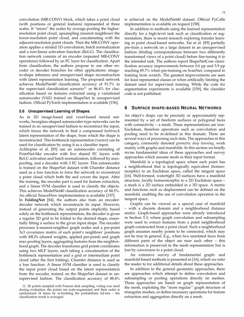
Fig. 1. Illustration of 3D representations used as neural network inputVolumetric grid (Section 3), Multiple-viewpoints renderings (Section 4),Point cloud (Section 5), and Mesh (included in Section 6). Exampleshape: ModelNet40 airplane 0627.

or LIDAR) which contain noise and occlusion. There are alsoworks which include an overview of classification methodsusing various representations of CAD models by Su et al.[13], Shen [14] and Wang et al. [15]. However, each papercontains only a few selected approaches. Bronstein et al. [16]provide a comprehensive review of methods working withnon-Euclidean input data – graphs and manifolds. Rostamiet al. [17] and Ahmed et al. [18] survey and categorizeapproaches also suitable for CAD models classification butinclude only a few recent deep-learning-based approaches.Compared to [18], we provide a more fine-grained catego-rization of classification approaches derived independentlyof their work but similar to their Input-oriented taxonomy.Several works also compare the practical performance ofvarious network architectures on a benchmark dataset –some only summarize the reported accuracies [9, 18, 19],while others replicate the performance evaluation and inde-pendently measure the accuracies [20, 21, 22].

1.2 Article StructureThe following sections 2 through 7 give an overview ofmethods using different shape representations and describeapproaches for each representation in detail. In sections8 and 9, we introduce our evaluation methodology andpresent the results of our experiments.

2 SURVEY OF 3D CLASSIFICATION METHODS

Shapes can be represented in various formats depending onthe use-case or data acquisition method. In CAD applica-tions, freeform surfaces or CSG (constructive solid geome-try) models are commonly used [23, 24], providing preciseinformation about object shape; other modeling softwareuses polygon mesh to represent the approximate shape ofthe object. In applications where the object is not createdon a computer, its shape is measured in real world usingsuitable sensors. In medical applications, computer tomog-raphy or magnetic resonance imaging are used to produce

volumetric scans, and in automotive and robotics industries,the object surface is scanned using an RGBD camera or a LI-DAR producing point clouds. Some reviewed classificationapproaches work with the native representation for theirdata source, others convert the original representation toanother format more suitable for processing with a neuralnetwork.

The usual approximative polygon or triangle mesh sur-face representation of 3D models in available datasets isnon-regular as triangle sizes may differ within a model andtriangle counts may differ between individual models, un-like e.g. images, where the resolution and pixel dimensionare fixed. Therefore such representation is a challenging in-put to be directly processed by a neural network commonlyworking with regularly structured input and only a fewnetworks use it as an input representation. Conversion toa different representation is often used to pre-process themesh to a more suitable format.

2.1 Categorization of Approaches

We provide a hierarchical categorization of the surveyedapproaches based on the following criteria. First, we classifythe networks according to the shape representation they useas their input: volumetric grid-based, multiple-viewpointimage-based, point cloud-based, networks which processthe object’s shape or mesh approximation, and hybrid meth-ods that process multiple representations simultaneously.Basic representation types are illustrated in Figure 1. Second,within each category, we couple the surveyed methods intocategories by the similarity of the used algorithms andapproach ideas and describe essential properties of eachmethod’s architecture. The resulting categorization is pre-sented in Table 1. Figure 2 shows the overview of reportedaccuracies.

Classification neural network architectures can be di-vided into two parts: a feature extractor, which transformsthe input shape representation to a feature vector, calleddescriptor, and a classifier, which learns to transform theextracted features into scores denoting the probability ofindividual classes. The feature extractor differs based on theinput representation and is usually designed based on eachapproach’s unique ideas. Depending on the approach, theseparts may be trained together (end-to-end) or separately.The following sections describe each representation in moredetail.

3 VOLUMETRIC GRID-BASED NEURAL NETWORKS

In volumetric convolutional neural networks (CNNs), theconvolution operation is used for the feature extraction task.It exploits the spatial locality of low-level features suchas edges and can be applied hierarchically, usually withpooling or striding, reducing the resolution and increasingthe level of abstraction in each step – similarly to CNNs thatprocess 2D images. As 2D convolutional neural networkswere a significant breakthrough in image classification [5],it is natural to generalize this approach to three dimensions.Instead of pixels, a 3D occupancy grid of volume elementsor voxels is used. However, the 3D convolution operationis computationally more demanding, and volumetric grids

3

Fig. 2. Reported accuracies of the surveyed methods over time. Datasets and input representations are denoted by different colors and shapes.

TABLE 1Taxonomy of the surveyed approaches. The references in bold were

included in our evaluation

Vol

umet

ric

grid

Basic Architectures [25] [26]Voxel CNN with Residual Connections [27] [28]Auxiliary Task [29]Network Architecture Optimization [30] [31] [32]Octree-represented Voxel Grid [33] [34] [35]Unsupervised Representation Learning [36] [37] [38] [39]Non-convolutional Approaches [40]Conversion from a Point Cloud [25] [41] [42]

Mul

ti-v

iew

(im

ages

) Basic Architectures [43] [44] [13]Multiple Modalities [45] [46]Axis-aligned Views [47] [48]Learned View Grouping [49] [50]Unsupervised Viewpoints Assignment [51] [52]Unsupervised Representation Learning [53]Using Auxiliary Data [54]

Special ProjectionsGeometry Images [55]Panorama [56] [57] [58] [59]Spherical [60]

Poin

tcl

oud

Symmetric Operation on Points [61] [62]Hierarchical Feature Extraction [63] [64] [65]Convolution on Neighborhood Graph [66] [67] [68]

Convolution on PointsGrid Around the Query Point [69] [70] [71]

Continuous Convolution [72] [73] [74] [75] [76][77] [78] [79]

Sequential Processing Using Attention Mechanism [80] [81]Encoding Locality into Order [82]

Unsupervised Learning of Shapes [83] [84] [85]

Surf

ace

shap

e Manifold-based Convolution [86] [87] [88]Graph-based Convolution [89] [90] [91] [92] [93]Native Mesh-based Approaches [94] [95] [96] [97]

Hyb

rid

Ensembling [98] [13] [20]Descriptor Merging [99]

tend to have high memory requirements as the voxel countgrows with the cube of the spatial resolution. For thisreason, only relatively low-resolution grids can be used, themost usual being 323.

Each voxel contains a value representing the presence ofthe object at a given place: several networks [25, 26, 31, 33]use a binary occupancy grid where each voxel is assumedto be either entirely occupied by the object (inside it) orempty (outside of the object). This format can be used forvoxelized watertight 3D meshes as the “is inside” predicateis well-defined. Another voxelization option is to occupyonly the voxels intersected by the object’s boundary (bothvoxels inside and outside of the object are empty), typical forvoxel grids converted from point clouds. Non-binary valuesmay be used for encoding the point cloud density [41], butthe difference in results is negligible [29]. Additional inputchannels such as surface normals may also be encoded ineach grid cell [34].

3.1 Basic ArchitecturesVoxNet [25] is the first of the successful systems applying3D convolutions to occupancy grids for classification, whichwe use as an example of a network with a convolutionalarchitecture. In VoxNet, the occupancy grid is processed bytwo 3D convolutional layers, which extract local featuresand lower the resolution. The convolution result is passedto a leaky ReLU layer to achieve nonlinearity. Maximumpooling is then performed to get better representation andfurther lower the number of parameters needed. Finally, theresulting 3D feature map is flattened and passed throughtwo fully connected layers, which output a vector withcategory probabilities. Figure 3 shows a diagram of theVoxNet architecture.

As is typical with neural networks, data augmentation isa crucial part of the training process. VoxNet uses rotationalong the vertical axis as its main augmentation technique.It uses n copies of each input instance during training, each

4

Occupancy Grid32x32x32

Conv(32,5,2)

14x14x14

Conv(32,3,1),Pool(2)

6x6x6 128

FC(128)

cScores

FC(c)

Fig. 3. VoxNet [25] architecture. c is the number of output categories.

rotated by 360/n degrees – typical values of n range from8 to 24. At evaluation time it presents all rotations of theinput object to the network and then uses pooling across therotations to get the class prediction. The authors reportedclassification accuracy of 83% on a subset of the ModelNet40dataset [26], which we briefly describe in Section 8.1. An offi-cial VoxNet implementation in Theano+Lasagne is available[100].

A similar 3D convolutional architecture is presented in3D ShapeNets [26]. It consists of 3 convolutional layersfollowed by a two-layer Restricted Boltzmann Machineclassifier. Apart from presenting a classification networkarchitecture, the authors also publish the ModelNet dataset.The reported classification accuracy on the ModelNet40subset is 77.32%. An official implementation in Matlab isavailable [101].

3.2 Voxel CNN with Residual Connections

Voxception-ResNet [27] is inspired by deep residual con-volutional networks for image classification, which are thestate-of-the-art approach for this task. It uses batch nor-malization [102] and residual connections [7]. The networkconsists of several sequential Voxception (Inception-style[103]) modules allowing stochastic network depth [104]between 8 and 45 layers, which should enable informa-tion to propagate in the network through many possible“pathways”. The best-performing architecture consists ofVoxception blocks and downsampling blocks, enabling theresidual network to choose the best downsampling methods(e.g., convolutions with stride greater than one or pooling).Voxel grid resolution of 323 is used. The network is trainedusing 24 rotations of each input instance along the verticalaxis and using occupancy grid with values {−1, 5} insteadof {0, 1} to encourage the network to pay more attentionto positive entries. Voxception-ResNet (VRN) architectureachieves 88.98% accuracy on ModelNet40 dataset for singlevoxelization view and 91.33% with 24 views. An ensembleof similar models achieves 95.54%, which remains one ofthe highest reported for voxel-based networks. The au-thors have published their implementation in Theano withLasagne [105].

Arvind et al. [28] explore the impact of residual layerwidth in volumetric networks on the classification accuracy.They show that increasing the number of channels in 3Dconvolutional layers improves the classification accuracy.This result extends the previous observations on residual 2Dconvolutional networks to 3D CNNs. They use a shallowerarchitecture consisting of one classical 3D convolution, max-pooling and two residual-convolutional blocks, each fol-lowed by two identity blocks (two single-voxel convolutions)acting as a two-layer perceptron with shared weights across

spatial dimensions, average pooling and a final classificationlayer. The best single-network model found by hyperpa-rameter grid search achieved 82.03% classification accuracyon ModelNet40, or 86.50% by ensembling 10 independenttraining sessions. As of writing, there is no implementationavailable.

3.3 Auxiliary TaskUsing an auxiliary task can improve classification accuracy.In the context of 3D CNNs, this has been shown in ORION[29] by simultaneously training the network for pose esti-mation. Apart from the object class, the network outputs ro-tation around the vertical axis. As different object categorieshave different rotational symmetries, the authors estimatethe orientation by classifying the canonical rotation, wherethe number of orientation classes is dependent on the objectcategory. This network achieves accuracy of 89.7% on theModelNet40 dataset with manual rotation alignment. Animplementation in Caffe and a manually-aligned version ofthe ModelNet40 dataset are available [106].

3.4 Network Architecture OptimizationAs the voxel representation and 3D CNNs are computation-ally demanding, there have been attempts to speed up thetraining and inference, such as manually or automaticallyoptimizing the number of layers or their hyper-parametersor replacing floating-point weights with binary values.LightNet [30] reduces the size of the VoxNet model byadding one more convolutional and max-pooling layer, re-ducing the resolution passed to the fully connected part ofthe network to 2×2×2 with 128 feature channels. LightNetalso uses multi-task learning: subvolume supervision and ori-entation estimation. Therefore there are two fully connectedclassifier branches: main and auxiliary, both outputtingthe category and 12-class orientation prediction. The mainbranch uses all the extracted features by the convolutionalpart, and consists of a two-layer perceptron with a finalsoftmax activation. The auxiliary branch consists of eightfully connected layers with softmax activation, each taking128 inputs – each from one voxel in the 2 × 2 × 2 featuremap – and outputting both the category and orientationprediction independently on the other parts of the auxiliarybranch. This forces the convolutional part of the network toextract meaningful features so that the class and orientationcan be determined even from parts of the input shape. Thefinal model has only 0.3M trainable parameters, less thana third of the original VoxNet architecture, while achievingsuperior ModelNet40 classification accuracy of 86.1%. Thecode was not publicly available as of writing.Xu and Todorovic [31] describe a process of automatic CNNarchitecture optimization by iterative layer or filter additionwhile keeping the trained weights. The best-performingarchitecture found by this approach consists of 3 convo-lutional layers followed by one fully connected (FC) layer.Compared to 3DShapeNets [26] the authors achieve betteraccuracy of 81.26% with less than 1% of the trainable pa-rameters. An official implementation in Matlab is available[107].Ma et al. [32] show the reduction of memory footprint andcomputational demands by converting layers inputs and

5

weights to binary values, adding necessary batch normal-ization layers and sign activation functions. Although inmost cases this process decreases the classification accuracy,in the case of binVoxNetPlus, a network constructed byadding one additional convolutional and a fully connectedlayer to VoxNet, the accuracy is increased by binarizationfrom 83.91% to 85.47% while the model size was just 0.29MB, approximately 8% of the original VoxNet. There was nopublic implementation at the time of writing.

3.5 Octree-represented Voxel Grid

As memory and computational demands limit the reso-lution of the voxel grid, a more efficient representationis needed to make processing a higher-resolution voxelgrid feasible. Voxel occupancy grids representing real-worldobjects or their surface are usually sparse; therefore, largeregions without changes in occupancy do not need to bestored or processed in full resolution.

Octree [108] is a tree where each internal node hasexactly eight children, partitioning the space into finer andfiner cubes (2 × 2 × 2) until a depth limit is reached orthe space corresponding to a node is homogeneous. Thisallows efficient voxelization of the 3D model where onlyvoxels on the object boundaries are stored at high resolution.Convolution and max-pooling can be adapted to work onoctrees. The octree structure can be processed efficientlyon GPUs when stored suitably, allowing fast training andinference.OctNet [33] uses octree to efficiently represent an occupancygrid, implementing convolution and pooling operations di-rectly on octrees. This reduces the memory and computa-tional requirements, allowing one of the presented modelsto process occupancy grids of 2563 resolution at memoryrequirements lower than if the model used the classicalvoxel representation at 643 resolution. The proposed net-work architecture consists of repeated blocks of two 33

convolutional layers and one max-pooling layer, halvingthe resolution until a 83 feature map is reached, which isthen passed to a fully connected classifier. The classificationperformance is on par with similar networks working witha dense voxel grid, achieving ModelNet40 classificationaccuracy of approximately 86.5% with 1283 input resolution.As the authors focused on measuring the impact of increas-ing the resolution, minimizing impact of other factors, a“pure” 3D CNN is proposed, unused methods such as dataaugmentation are likely to further improve the performance.An official implementation in Torch is available [109].O-CNN [34] uses octree to store the object surface, withadditional information: normal vector of the surface storedin leaf nodes. The authors present an efficient convolutionoperation on octrees and construct a hierarchical structureof shared layers for individual levels of the tree. Globalfeature computation proceeds from the finest leaf octantsand continues upwards to the root of the tree. The high-level O-CNN architecture used for classification consistsof repeated 3D convolutions and max-pooling followed bytwo fully connected layers with dropout and a final soft-max activation. The O-CNN with five convolutional layersprocessing the input with resolution of 643 achieved 89.9%in ModelNet40 classification accuracy for single input and

90.6% with 12-rotation voting. Standard octrees have a fixedmaximum depth, wasting memory on flat regions where asimple planar approximation would be sufficient. AdaptiveOctree representation used in Adaptive O-CNN [35] usesplanar patches as a representation in leaf nodes. Flat areasof the original mesh can be represented by a single leafon a higher level of the tree, while more complex areasare subdivided into finer details. Both computation timeand memory requirements are reduced compared to the O-CNN network, in case of the 2563 input resolution, wherethe change is the most significant, to approximately 1/4.Apart from the convolutional encoder for feature extraction,a decoder is also proposed, allowing other tasks such as 3Dautoencoding and shape completion. The achieved Model-Net40 classification accuracy is 90.5% with 12-orientationvoting with input resolution of 323. The authors offer animplementation of both networks in Caffe and tools forconverting mesh data to octrees and adaptive octrees [110].

3.6 Unsupervised Representation LearningAll approaches described so far learn features for clas-sification in a supervised training scenario – providingthe correct category labels to the network when runningback-propagation training pass. This section describes ap-proaches with an additional training step – unsupervisedlearning of features on a different task such as reconstruc-tion of the input, using an auto-encoder, to force the networkto find a meaningful latent space or “bottleneck” represen-tation. The input-to-latent-space mapping learned by theencoder can be used for feature extraction. In the next step,a classifier can be trained to transform these features intocategory labels of the input object in a supervised fashion.The classifier can be either a separate model (e.g. SVM ora neural network), or the decoder can be replaced withe.g. a fully connected classifier, and the network can betrained end-to-end, fine-tuning the previously found input-to-latent-space mapping.VConv-DAE [36] is the first attempt to learn a shape embed-ding in an unsupervised way. The authors use a denoisingautoencoder with two convolutional (and de-convolutional)layers that aims to learn a 6912-dimensional latent represen-tation of training shapes. After training the autoencoder ona subset of ModelNet dataset the authors compare followingtwo approaches for classification: using an SVM classifier, orattaching two fully connected layers after the encoder andfine-tuning the network end-to-end. The former approachachieves 75.50% ModelNet402 classification accuracy, prov-ing the network found some category-identifying featureson its own. The fine-tuned model achieved 79.84%. Anofficial implementation in Torch is available [111].3D-GAN [37] is a fully 3D-convolutional generative adver-sarial network [112] with a 5 convolutional layers generatorand discriminator trained on voxelized models from theShapeNetCore dataset. Concatenation of several discrimi-nator layers’ outputs (max-pooled 2., 3. and 4.) is passedto linear SVM for classification. This model achieves 83.3%classification accuracy on the ModelNet40 dataset. The au-thors provide an implementation in Torch [113].

2. Using a ModelNet40 subset with equal category model counts andtherefore different train/test split.

6

Wang et al. [38] present 3D-ED-GAN, a combination of3+3 convolutional layers encoder-decoder with adversarialloss (discriminator) trained to reconstruct damaged, lower-resolution input. Although the authors focus mainly oninpainting, the encoder part of the network is used forclassification in one of the presented experiments. Whenusing only the encoder to extract features, passing themto a linear SVM, the ModelNet40 classification accuracy of84.3% is achieved. The ModelNet40 classification accuracyof 87.3% is achieved with pre-training the encoder-decoderon ShapeNetCore in an unsupervised fashion, then usingthe latent representation as input of a classifier with softmaxactivation. When the same model was trained from scratch(without pre-training, with randomly initialized weights)the accuracy of 86.1% was achieved, 1.2 pp lower thanthe fine-tuned result. As of writing, only an unofficial3

implementation in TensorFlow is available [114].Variational Shape Learner [39] is a variational encoder-decoder learning the latent representations of shapes inan unsupervised fashion and using the representation forclassification. Apart from producing just one global featurevector (latent code) by passing the input voxel occupancygrid through three convolutional layers followed by twoFC layers, local latent codes are also computed. Each localfeature is computed by two FC layers, whose input is theconcatenation of a sample of the global feature vector andthe previous local latent code – the output of the previouslocal layer, if any. The authors argue this approach helps thenetwork better learn a hierarchical representation of inputshapes, where each local feature vector represents a higherlevel of abstraction. This approach achieves 84.5% accuracyon ModelNet40 by training an SVM on extracted features– concatenated global and local latent features. An officialTensorFlow source code is available [115].

3.7 Non-convolutional ApproachesFPNN [40] presents a lightweight, non-rigid alternative toconvolution. Compared to convolution, the weights at givenpositions are optimized together with the positions of theprobing points. First the voxel occupancy grid is convertedto a 3D distance field – a voxel grid containing values repre-senting a continuous distance from the surface; distance atarbitrary position is computed as a tri-linear approximationusing nearest cells. The distance field is “sensed” withprobing points (filters), whose weights and positions arelearned. The distances at probed positions and the trainedweights are combined by dot product. Similarly to the objectshape being represented with a distance field, normals arestored in a three-channel normal field. The proposed non-hierarchical architecture passes the distance and normalfields through field probing layers, producing an internalrepresentation of the input shape, from which the objectclass is extracted with fully connected layers. This approachachieves 88.4% ModelNet40 classification accuracy with 4fully connected layers at the end, with distance field andnormals on input, or 87.5% without the normal field. Anofficial implementation in Caffe is available [116].

3. Differs from the paper: needs modification to extract the latentrepresentation for classification, last decoder layer has 512 filters, not256 as in the paper, possibly other differences.

3.8 Conversion from a Point Cloud

Point cloud processing with a convolutional neural networkis not trivial, as the standard convolution requires its inputto be a regular grid. There are approaches which take a pointcloud as input, convert it to a voxel grid, and apply 3D con-volutions for feature extraction followed by classification.VoxNet, which was mentioned earlier, uses a voxel occu-pancy grid generated from a point cloud input, passing thevoxel grid to the CNN’s input.PointNet by Garcia-Garcia et al. [41]4 integrates the pointcloud to occupancy grid conversion into the network asa non-trainable layer. The grid representation is then pro-cessed like in other voxel-based networks by repeated 3Dconvolutions and pooling followed by a 3-layer perceptron.PointGrid [42] achieves input regularity by sampling apredefined number of points from the input point cloudin each cell of a regular 3D occupancy grid, concatenatingrelative coordinates of the sampled points in each voxel,so they can be used as features of the voxel. The rest ofthe model consists of 9 3D convolutions and max-poolingfollowed by FC layers. This architecture achieves 92.0%ModelNet40 classification accuracy and 86.1% accuracy onthe ShapeNetCore dataset. The official source code writtenin TensorFlow is available [117].

4 MULTIPLE-VIEWPOINT IMAGE-BASED NEURALNETWORKS

Multi-view image-based networks use 2D images of theobject as input, captured or rendered from different view-points. A general setup of a multi-view classification net-work is as follows: the images (views of a single 3D shape)are passed to one or more feature extractors, then a tech-nique for combining features from different views is em-ployed, and the resulting feature vector is sent to a classifier.Feature combining techniques range from simple poolingacross the views to employing a recurrent neural network toprocess them as a sequence. Being based on image featureextractors allows reusing existing image-processing CNNs,enabling transfer learning and leading to good results.

The individual multi-view approaches generally differin several aspects: the number of viewpoints and their spa-tial distribution, input modality, whether they use multiplemodalities generated from each viewpoint, which 2D CNNarchitecture they use for image feature extraction, whetherthe weights are shared among viewpoints, and in the way,they aggregate the features extracted from the renderedimages.

4.1 Basic Architectures

The first multi-view CNN approach for 3D object classifi-cation by Lecun and Huang [43] uses two views as input(simulating binocular vision), which are sent to a shallowconvolutional neural network. The architecture consists ofthree convolutional layers with intermediary sub-samplinglayers, followed by one fully connected layer, which predictscategory probability vector. Half of the convolutional filtersin the first layer are applied to only one of the two images

4. Not to be confused with the PointNet by Qi et al. [61].

7

Fig. 4. Multi-view architecture [44], as used in [13]. The numbers belowthe diagram denote tensor sizes; c is the number of output categories.

(left or right), the other half process both. All features arethen merged in the last convolutional layer. As this workpredates the ModelNet dataset, it has only been evaluatedon a dataset of physical uniform-colored toys photos withvarying viewpoints and lighting, released with the paper.

The first approach to process more than two views forclassification is MVCNN [44]. It uses feature extractorsbased on VGG [6], sharing weights for individual viewpointbranches, then applies max pooling across the views tocombine the extracted features. Resulting feature vector ispassed to three sequential fully connected layers for clas-sification. When training, the network is first trained as asingle-view classification network (single feature extractionbranch, without max pooling), then other view branchesare added and the network weights are fine-tuned. Theauthors use two different viewpoint configurations: either12 “turntable” views5 or 80 virtual cameras placed in 20vertices of a dodecahedron around the object, each with 4rotations in 90 degree increments to detect objects with non-upright pose. The 12-view network achieves ModelNet406

classification accuracy of 89.9% with pre-training on Ima-geNet, and the 80-view variant achieves 90.1%. The authorspublished an implementation in Matlab [118].

A revisited but similar approach is presented by Su et al.[13]. The authors explore different pre-trained image net-work architectures and image rendering techniques, sig-nificantly improving accuracy of this method. The best-performing classification model takes 12 Phong-shaded im-ages as input uses a pre-trained ResNet-34 convolutionalnetwork as its base, and achieves 95.9% accuracy on theModelNet40 benchmark. When the VGG network is used forfeature extraction, the accuracy of 95.0% is achieved whenfine-tuning its weights initially trained on ImageNet1K, and91.3% without pre-training. The authors also tried usingdepth images concatenated to the shaded images, whichyields 96.2% classification accuracy. An illustration of themulti-view architecture is shown in Figure 4. The authorsoffer a publicly available PyTorch implementation[119], uti-lizing the VGG CNN as the feature extractor.

5. Twelve virtual cameras regularly distributed at 30-degree elevationfrom the object centroid.

6. Limited to 100 shapes per category; published dataset: 3983 shapes.

4.2 Multiple ModalitiesThe classification accuracy may benefit from extra informa-tion in addition to the shaded images, such as depth or sur-face curvature, passed as additional images to separately-trained feature extraction branches of the network. Thereare more approaches based on this idea.Johns et al. [45] process a pair of images in two modalities(shaded and depth) from multiple viewpoints. The imagesare processed with a CNN to extract features passed toa 3-layer fully connected network to predict a class labeland next-best-view viewpoints. This model achieves Model-Net40 classification accuracy of 89.5% (6 viewpoints chosenby the network) or 92.0% (12 views). No code was availableat the time of writing.The classification approach described by Minto et al. [46]uses axis-aligned images with multiple rendered modalities:depth, voxel density (X-ray-like image), and estimated sur-face curvature constructed by fitting a parametric surface(NURBS) to the points constructed from depth-image sam-ples. The images are passed to a 4- or 5-layer CNN, whoseweights are shared among branches processing the imagesof the same modality, which are rendered from viewpointsrotated around the vertical axis. The extracted features arethen concatenated and passed to a fully connected layerwith a softmax activation for classification. This achieves89.3% classification accuracy on ModelNet40. No code wasavailable at the time of writing.

4.3 Axis-aligned ViewsSome approaches restrict the camera positions to only axis-aligned viewpoints, while using one modality.Zanuttigh and Minto [47] use six axis-aligned depth imagesrendered from coordinate axis directions, looking towardthe origin. The images are passed to CNNs consisting offour 7 × 7 convolutions, in a branch for each view, sharingweights for rotations around the vertical axis. The featureextractors’ outputs are concatenated and sent to a single-layer classifier. This approach yields ModelNet40 classifica-tion accuracy of 87.8%. No code was available at the time ofwriting.Sarkar et al. [48] propose to use multi-layer heightmaps asan input image modality. Multi-layer heightmaps are depthimages rendered from multiple planar slices through the ob-ject, in this case, axis-aligned. Three views with a heightmapof each slice, stored as individual channels, are passed toVGG16 (with batch normalization, without FC layers), theresulting features are then merged by concatenation alongthe depth or channel dimension to preserve the informationabout which feature comes from which view. A convolu-tional layer then reduces the channel count, and the featuresare passed to one FC layer for classification. This modelachieves 93.11% classification accuracy on ModelNet40 with5-layer heightmaps and VGG CNN pretrained on ImageNet.The authors have published their PyTorch code [120].

4.4 Learned View GroupingRather than using simple max- or average-pooling to aggre-gate features from multiple viewpoints, these approachesuse a trainable model, promising to learn to use the mostimportant features from each view.

8

GVCNN [49] adds a view-grouping step between the ex-tracted features and the classifier, considering the correla-tion among individual views. The features are extracted bypassing each view (shaded image) through the first fiveconvolutional layers of GoogLeNet7 independently. Thenper-view discrimination scores are computed by pooling theextracted features, and views are assigned to groups basedon their discrimination scores – quantized to bins expressing“how well does this view perform in classification”. Thenthe view groups are pooled using a grouping scheme, whichis selected based on the final group count. On ModelNet40this approach achieves 93.1% accuracy with 8 views, pre-trained on ImageNet1K. The authors have not publishedthe code, but there are two unofficial implementations: inTensorFlow [121] and in PyTorch [122].SeqViews2SeqLabels [50] employs a recurrent neural net-work and treats multiple views as a sequence of imagesusing an encoder-decoder architecture. The network outputsa sequence of class labels rather than probability vectors.A pre-trained VGG-19 network, fine-tuned on the single-image classification task, is used as per-view feature extrac-tor. Feature vectors are fed into the encoder as a sequence.Both the encoder and decoder consist of GRU cells [123]; at-tention is used in the decoder for selecting distinctive viewsfor current output label. This architecture achieves 93.31%classification accuracy on ModelNet40. An implementationin TensorFlow is available [124].

4.5 Unsupervised Viewpoints Assignment

Unlike other multi-view networks, these networks do notobtain information about the position of the viewpoints, i.e.,the viewpoints can be rotated arbitrarily. It is the task of thenetwork to find a suitable assignment of input images toviewpoints.RotationNet [51] combines the multi-view classificationwith an unsupervised pose estimation task. This encouragesthe network to train one CNN per viewpoint to classifythe object in an input image from a specific viewpoint. Anew category is added to the set of original classificationcategories to assess the image-to-viewpoint assignment’scorrectness. The meaning of this category is “this is not thecorrect viewpoint”. Such per-viewpoint training helps theCNNs by reducing the input image variations, allowing thetrained convolutional filters to be more view-specific. Theimage-to-viewpoint assignment is trained in an unsuper-vised fashion, trying multiple assignments during inference,choosing the most probable one8 according to predictedcategories. The authors report maximum accuracy of 97.37%on the same subset of ModelNet40 dataset as used in [44].The authors published two implementations, one in Caffe[125], and another one in PyTorch [126].Sarkar et al. [52] present a RotationNet-like network trainedon images produced by rendering slices of the input model.They render multi-layer heightmaps or occupancy slicesimages – a binary image representing intersections of the

7. GoogLeNet = Inception v1, but Inception v4 is used in bothavailable unofficial implementations

8. The one with the least probability of being in the “incorrectviewpoint” category

model with the slicing plane. The authors report the ac-curacy on ModelNet40 of 99.76% when using 12 turntableviews in occupancy slices modality with 10 slices. The codehad not been published at the time of writing.

4.6 Unsupervised Representation Learning

Like in the case of volumetric networks, the classificationcan be achieved by first training an auto-encoder networkin an unsupervised fashion, and then using the bottleneckrepresentation as extracted features, only appending a clas-sifier.Soltani et al. [53] use unsupervised representation learningworking on images of one of multiple modalities. The au-thors use a variational autoencoder built from four residualconvolution blocks in the encoder, working with multi-viewdepth maps or silhouettes rendered from 20 viewpointsin dodecahedron vertices. While not focusing on reachingstate-of-the-art classification accuracy, the proposed AllVP-Net architecture with two-layer dense classifier appended tothe encoder achieves ModelNet40 classification accuracy of82.1% and 89.1% on their split of ShapeNetCore, both withdepth images used as input. No fine-tuning was used. Theauthors offer an implementation in Torch [127].

4.7 Using Auxiliary Data

Some 3D shape datasets provide part segmentation infor-mation useful to aid further the classification process.Parts4Feature [54] proposes using local part detection byextracting features from each view and using a region pro-posal network [128] to produce a representation of possibleparts visible in each view. For classification, top k proposedregions are aggregated by an attention mechanism and partco-occurrence patterns learning. Using part segmentationinformation during training, the model achieves 93.40%accuracy on ModelNet40 and 86.9% on the ShapeNetCoredataset. No code was available at the time of writing.

4.8 Special Projections

There are also approaches which use other projections thanperspective or planar projections from multiple viewpoints,described earlier.

4.8.1 Geometry Images

A 2-manifold 3D mesh can be represented as a so-calledgeometry image by cutting the mesh along edges andmapping the unwrapped mesh into a square image domaincontaining channels representing the original coordinatesand local properties such as curvature. Sinha et al. [55] takea geometry image of 56 × 56 pixels as an input with thefollowing channels: two principal curvatures, topologicalmask and height field. The proposed CNN extracts a 96-dimensional feature vector from the image, which is passedto a fully connected layer for classification. The approachachieves ModelNet40 classification accuracy of 83.9%. Thecode for generating geometry images has been published[129], but we have not found the code for the CNN or itstraining.

9

4.8.2 Panorama Projection

Another projection of a 3D shape suitable for CNNs is apanoramic view. DeepPano [56] uses a single view of the3D shape: a depth image created by cylindrical projectionaround the vertical axis, passed to a 4-layer CNN, row-wise max-pooling for rotation invariance, and two fullyconnected layers and softmax-activated output. This modelachieves 82.54% classification accuracy on ModelNet40. Theauthors have published their Matlab code for panoramaprojection image rendering [130], but not the CNN imple-mentation.Another approach by Sfikas et al. [57] uses three views:rendering each model in cylindrical projection along eachaxis. Depth and normals’ deviation map modalities arestored as image channels. Image features are extracted witha 3-convolutional-layer CNN and classified with one fullyconnected layer, dropout layer and softmax activation. Theobject pose is normalized before rendering. The classifica-tion accuracy of 90.70% is achieved on the ModelNet40dataset. No public implementation is available.In a follow-up paper, Sfikas et al. [58] also use three views:cylindrical projections corresponding to major axes withan additional modality: the magnitude of the normals’deviation map gradient. The architecture is identical to theprevious model, except it has two fully connected layers in-stead of one. The authors achieve ModelNet40 classificationaccuracy of 95.56%. No code was available at the time ofwriting.Cao et al. [59] use 12 views: vertical stripe-projectionsaround the sphere (parallel to longitudes) and one horizon-tal stripe (cylindrical projection). The vertical slice imagesare fed into a MVCNN-like network with AlexNet featureextraction; similarly, a feature vector is extracted from thehorizontal stripe. Finally, the two feature vectors are con-catenated and passed to a fully connected layer with soft-max activation for classification. Using depth and contoursmodalities the network achieves 94.24% classification accu-racy on ModelNet40 and 91.00% on ShapeNetCore, bothfine-tuning AlexNet weights pre-trained on the ImageNetdataset. No code was available at the time of writing.

4.8.3 Spherical Representation

The input shape can also be projected into a sphericaldomain and passed to a CNN with operations workingin that domain. Spherical CNN [60] computes a sphericalfunction similar to a depth map – distance to the firstintersection of a ray cast from a point on an enclosing spheretoward the origin – and surface normals at the intersectionpoints. Convolutions in the spherical harmonic domain areapplied, and spectral pooling is used for rotation invariance.The architecture consists of two branches, one for eachmodality, each with 8 spherical-convolutional layers. Theextracted features are then pooled, concatenated and passedto a classifier. This achieves ModelNet40 classification accu-racy of 88.9% when only z-rotation invariance is required,and 86.9% for full SO(3) rotation invariance. The authorspublished an implementation in TensorFlow and code toconvert voxel occupancy grids to spherical domain [131],but no code for mesh projection.

5 POINT-CLOUD-BASED NEURAL NETWORKS

A point cloud is a set of points in Euclidean space represent-ing the surface of the object. It is a natural output formatof laser scanning devices used by robots or autonomouscars. It can also be easily constructed from an artificially-modeled object by sampling its surface, e.g. mesh faces.Compared to volumetric grids or images, point clouds areneither structured nor ordered, which poses a challenge toneural networks: point-based operations need to be definedfor successful feature extraction. Unlike VoxNet [25] andPointNet by Garcia-Garcia et al. [41] presented above, whichconvert the input point cloud to a dense volumetric grid andapply 3D convolutions, this section describes architectureswhich work directly with a set of point coordinates ora derived representation maintaining its unstructured andnon-dense nature.

The approaches working with this representation differthe most in the feature extraction methods. Some processeach point individually and apply a symmetric aggregationoperation to achieve order-invariance. Others construct anearest-neighbor graph and extract features from that, ordefine a convolution-like operation working with points bygeneralizing the input and kernel to non-rigid positions.

5.1 Symmetric Operation on PointsOne of the first networks to successfully overcome thedifficulties of processing raw unordered point clouds isPointNet by Qi et al. [61]. Its main idea lies in using onlysymmetric functions, i.e., functions for which the order ofarguments does not matter. Each point is processed in-dependently by a series of multi-layer perceptrons (MLP)sharing their weights. Then a global feature vector is con-structed using max-pooling, which is a symmetric function.Another important feature of PointNet is the set of learnablegeometric transformations, which ensure some invarianceto rotation or jittering (random small translations) of theinput point cloud. Rotation and jittering are also used asdata augmentation during the training. Figure 5 shows thediagram of the PointNet architecture. The authors reportModelNet40 classification accuracy of 89.2% on 1024 points.A TensorFlow implementation of this network is available[132]. The PointNet architecture (without T-Net blocks) isalso implemented in Minkowski Engine [133], a generic ma-chine learning and auto-differentiation framework support-ing sparse tensors, which allows training and evaluationusing different number of points in each object.Deep Sets [62] is a concurrent research based on the sameidea of using a symmetric function for points aggregation.In the proposed classification network, each input point istransformed independently into a learned internal represen-tation by three dense layers with tanh non-linearity. Thenmax-pooling is used, which is a symmetric operation as inPointNet. The resulting vector is processed with two denselayers for classification. This model achieves ModelNet40classification accuracy of 90.0%± 0.3% for 5000 points or87%± 1% for 1000 points. An official implementation inPyTorch is available [134].

Although PointNet and Deep Sets achieve better classi-fication accuracy than previous methods based on manu-ally designed feature extractors, the performance was later

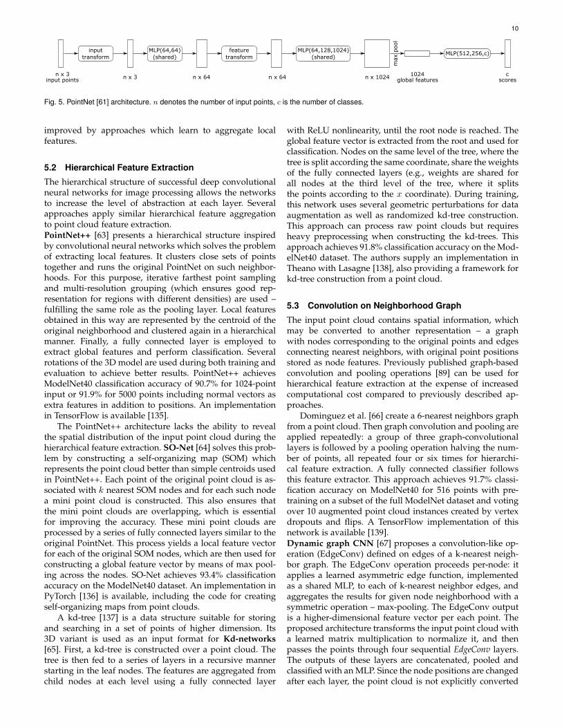
10

Fig. 5. PointNet [61] architecture. n denotes the number of input points, c is the number of classes.

improved by approaches which learn to aggregate localfeatures.

5.2 Hierarchical Feature Extraction

The hierarchical structure of successful deep convolutionalneural networks for image processing allows the networksto increase the level of abstraction at each layer. Severalapproaches apply similar hierarchical feature aggregationto point cloud feature extraction.PointNet++ [63] presents a hierarchical structure inspiredby convolutional neural networks which solves the problemof extracting local features. It clusters close sets of pointstogether and runs the original PointNet on such neighbor-hoods. For this purpose, iterative farthest point samplingand multi-resolution grouping (which ensures good rep-resentation for regions with different densities) are used –fulfilling the same role as the pooling layer. Local featuresobtained in this way are represented by the centroid of theoriginal neighborhood and clustered again in a hierarchicalmanner. Finally, a fully connected layer is employed toextract global features and perform classification. Severalrotations of the 3D model are used during both training andevaluation to achieve better results. PointNet++ achievesModelNet40 classification accuracy of 90.7% for 1024-pointinput or 91.9% for 5000 points including normal vectors asextra features in addition to positions. An implementationin TensorFlow is available [135].

The PointNet++ architecture lacks the ability to revealthe spatial distribution of the input point cloud during thehierarchical feature extraction. SO-Net [64] solves this prob-lem by constructing a self-organizing map (SOM) whichrepresents the point cloud better than simple centroids usedin PointNet++. Each point of the original point cloud is as-sociated with k nearest SOM nodes and for each such nodea mini point cloud is constructed. This also ensures thatthe mini point clouds are overlapping, which is essentialfor improving the accuracy. These mini point clouds areprocessed by a series of fully connected layers similar to theoriginal PointNet. This process yields a local feature vectorfor each of the original SOM nodes, which are then used forconstructing a global feature vector by means of max pool-ing across the nodes. SO-Net achieves 93.4% classificationaccuracy on the ModelNet40 dataset. An implementation inPyTorch [136] is available, including the code for creatingself-organizing maps from point clouds.

A kd-tree [137] is a data structure suitable for storingand searching in a set of points of higher dimension. Its3D variant is used as an input format for Kd-networks[65]. First, a kd-tree is constructed over a point cloud. Thetree is then fed to a series of layers in a recursive mannerstarting in the leaf nodes. The features are aggregated fromchild nodes at each level using a fully connected layer

with ReLU nonlinearity, until the root node is reached. Theglobal feature vector is extracted from the root and used forclassification. Nodes on the same level of the tree, where thetree is split according the same coordinate, share the weightsof the fully connected layers (e.g., weights are shared forall nodes at the third level of the tree, where it splitsthe points according to the x coordinate). During training,this network uses several geometric perturbations for dataaugmentation as well as randomized kd-tree construction.This approach can process raw point clouds but requiresheavy preprocessing when constructing the kd-trees. Thisapproach achieves 91.8% classification accuracy on the Mod-elNet40 dataset. The authors supply an implementation inTheano with Lasagne [138], also providing a framework forkd-tree construction from a point cloud.

5.3 Convolution on Neighborhood Graph

The input point cloud contains spatial information, whichmay be converted to another representation – a graphwith nodes corresponding to the original points and edgesconnecting nearest neighbors, with original point positionsstored as node features. Previously published graph-basedconvolution and pooling operations [89] can be used forhierarchical feature extraction at the expense of increasedcomputational cost compared to previously described ap-proaches.

Dominguez et al. [66] create a 6-nearest neighbors graphfrom a point cloud. Then graph convolution and pooling areapplied repeatedly: a group of three graph-convolutionallayers is followed by a pooling operation halving the num-ber of points, all repeated four or six times for hierarchi-cal feature extraction. A fully connected classifier followsthis feature extractor. This approach achieves 91.7% classi-fication accuracy on ModelNet40 for 516 points with pre-training on a subset of the full ModelNet dataset and votingover 10 augmented point cloud instances created by vertexdropouts and flips. A TensorFlow implementation of thisnetwork is available [139].Dynamic graph CNN [67] proposes a convolution-like op-eration (EdgeConv) defined on edges of a k-nearest neigh-bor graph. The EdgeConv operation proceeds per-node: itapplies a learned asymmetric edge function, implementedas a shared MLP, to each of k-nearest neighbor edges, andaggregates the results for given node neighborhood with asymmetric operation – max-pooling. The EdgeConv outputis a higher-dimensional feature vector per each point. Theproposed architecture transforms the input point cloud witha learned matrix multiplication to normalize it, and thenpasses the points through four sequential EdgeConv layers.The outputs of these layers are concatenated, pooled andclassified with an MLP. Since the node positions are changedafter each layer, the point cloud is not explicitly converted

11

to a graph representation – the graph is constructed “on de-mand” as needed from a set of points passed between layers.This approach achieves ModelNet40 classification accuracyof 92.9% for 1024-point input or 93.5% when sampled with2048 points. Implementations in PyTorch and TensorFloware available [140].

Lei et al. [68] propose efficient graph convolution andpooling operations on neighborhood graphs. The convolu-tion kernel uses binning in discretized spherical coordinatessimilar to [70] weights are selected based on the positionrelative to the query point. Graph coarsening using farthestpoint sampling (to select point set of desired size to remainin the graph) is used to construct a multi-resolution pyramidof graphs; between its layers the convolution kernels are ap-plied. Similarly, the order of pyramid layers can be reversedfor upsampling. A classification network consisting of three-level pyramid encoder, global feature extraction and a fullyconnected classifier achieves ModelNet40 classification ac-curacy of 91.4% on 2048 points and 92.1% on 10000 points.A TensorFlow implementation is available [141].

5.4 Defining Convolution on Points

Similar to volumetric grid-based neural networks drawingfrom image CNNs, there have been successful attemptsto adapt the convolution operation to work with pointclouds. As in these networks, the convolution operationcomputes local activation as an aggregated product of alearned kernel and the neighborhood of each query pointin the input. However, unlike voxel networks, the pointconvolution cannot assume a regular input (e.g. uniformdensity of the point cloud), but may use a regular kernel andpoint binning when computing the activation. In additionto the convolution operation, the pooling and sub-samplingoperations also need to be adapted to point clouds to allowhierarchical feature extraction.

5.4.1 “Grid” Around the Query PointIn the following approaches, the kernel is a spatial structurecentered at the position of the query point. The input pointsare binned in a grid based on their relative position from thequery point, and weights are learned for the grid cells.

Hua et al. [69] define a pointwise convolution operator,which is applied at each point position, which essentiallyvoxelizes a local neighborhood. The pointwise convolutioncenters a kernel at the currently processed point and binsclose points to a regular grid around current point, ag-gregating point features in each cell, then a regular 3Dconvolution is used. To reduce the dependency on the inputpoints permutation, the authors propose sorting the pointsin a canonical ordering (Morton curve). In the proposedclassification network, the intermediate results from all fourconvolutional layers are concatenated and passed throughtwo FC layers for classification. This achieves ModelNet40classification accuracy of 86.1%. An official implementationin TensorFlow is available [142].

The spatial structure does not need to be a regulargrid. Xie et al. [70] propose a convolution kernel wherethe current point neighborhood in relative radial coordinatesystem is split into a predefined number of bins in eachcoordinate. E.g. there are 8 quadrant bins with trainable

weights for 2 polar and 4 azimuthal splits and no radialsplit. Points in each bin are aggregated by sum-pooling andthe resulting per-bin vectors are transformed to a featurevector of the desired dimensionality. The best classificationmodel consists of 5 ShapeContext layers, max-pooling anda MLP classifier. This approach achieves 90.0% accuracy onModelNet40 for 1024 points, 27-bin kernels (3 azimuthal ×3 polar × 3 radial, max. radius = 0.5) or 89.8% for a learningmodel, where the bins are not hand-crafted, but the pointsare processed with a self-attention block. There was no codeavailable at the time of writing.

Another option outlined in A-CNN [71] is to computea convolution of points in a ring around a point. The orderof points is “normalized” by sorting them counter-clockwisewhen querying for point neighbors inside a ring after projec-tion to an estimated tangent plane. The annular convolutionis a 1D convolution of a 1 × k kernel and the orderedneighbors in a ring. The authors argue that compared tomulti-scale neighborhood extraction (e.g. in PointNet++) theproposed ring approach does not have overlaps of indi-vidual areas at different scales, allowing the weights to beoptimized using more discriminative, less redundant data.The classification network consists of repeated farthest pointsubsampling and annular convolutions to increase the re-ceptive field of the extracted features, max-pooling and MLPfor classification. The trained model achieves ModelNet40classification accuracy of 92.6%. Authors’ implementationin TensorFlow is provided [143].

5.4.2 Continuous ConvolutionRather than defining a discrete spatial structure, the convo-lution operation can be naturally defined on a continuousdomain. The following approaches outline some of thepossible definitions.

Point Convolutional Neural Networks [72] define a con-volution operation on point clouds by extending the func-tion defined over the point cloud to continuous 3D space.Then the classical convolution operation is applied, and theresult is converted back to a point cloud by sampling. Theproposed classificaton network consists of 3 convolutionallayers followed by two FC layers. The classification accuracyon ModelNet40 is 92.3% with 1024 points. An implementa-tion in TensorFlow is available [144].

Shen et al. [73] propose a kernel correlation layer, aconvolution-like operation on point sets producing activa-tions based on the correspondence of the kernel and thequery point neighborhood. The kernel is a set of pointswith learnable positions. The classification network modelextracts the low-level features by kernel correlation for eachpoint, concatenates them with input points’ positions andpasses the result through a series of MLPs with a concate-nated graph max-pooling “side-branch” to aggregate localfeatures of nearby points. The model achieves ModelNet40classification accuracy of 91.0%. The authors’ implementa-tion in Caffe is available on request [145].KPConv [74] also uses a kernel consisting of a set of pointswith learnable positions and also weights. The proposed 5-layer classification networks achieve 92.9% and 92.7% clas-sification accuracy for rigid and deformable kernels, respec-tively. An official TensorFlow implementation is available[146].

12

PointConv [75] is another approximation of continuousconvolution by a set of points. To approximate continuousweight functions, MLP is used and weights are compen-sated for non-uniform point density: features∗weights

density . Theclassification architecture consists of a feature extractor with4 pointwise-convolution layers and a 3-layer perceptron.The authors report ModelNet40 classification accuracy of92.5% when using 1024 points with normals. An officialPyTorch implementation is available [147].SpiderCNN [76] also proposes a continuous kernel general-ization. The learnable kernels are based on step function andTaylor polynomials – to reduce the number of parametersneeded in contrast with MLP. The best-performing classi-fication network consists of 4 SpiderConv layers, whoseoutputs are concatenated, top-2-pooled and passed to a MLPclassifier. SpiderCNN achieves ModelNet40 classificationaccuracy of 92.4%. A TensorFlow implementation of thearchitecture was published by the authors [148].PointCNN [77] introduces a X -Conv operator – a methodapplying a typical convolution to point clouds by firstweighting and permuting input features with a learnedtransformation of the point coordinates relative to the querypoint. The X -transformation is based on an MLP, whichlearns the weights of individual points and their latent or-der. The classification network consists of two X -Conv lay-ers subsampled with dilation d: instead of passing k nearestneighbors to the X -Conv, k ∗ d nearest neighbors are foundand k points are sampled from them. The X -Conv layersare followed by four FC layer branches, each using differentoutputs of the last X -Conv layer. The FC branch outputs areaveraged during evaluation. The proposed model achieves92.2% classification accuracy on ModelNet40 and 92.5% onrotation-aligned ModelNet40. An official implementation inTensorFlow is available [149].Flex-Convolution [78] focuses on reducing computationaland memory requirements, allowing large9 point clouds tobe processed. The simplified kernel is linear in each dimen-sion – a dot-product of a trainable parameter vector andpoint’s relative coordinates, with trainable bias added. Theused point sub-sampling is random sampling weighted bylocal point cloud density. The authors achieve ModelNet40classification accuracy of 90.2% (for 1024 points). Authors’implementation in TensorFlow is available [150].Another continuous convolution with a spherical neighbor-hood kernel is presented by Liu et al. [79]. A 3-layer MLPcomputes the weights from a vector of low-level relations ofthe query point (centroid) and each point in the neighbor-hood: Euclidean distance, coordinate difference and pointposition. The classification network uses three convolutionallayers and a MLP classifier. This model achieved Model-Net40 classification accuracy of 93.6% for 1024 points withvoting across 10 random scales. An official implementationin PyTorch is available [151].

5.5 Sequential Point Cloud Processing

Processing the point cloud as a sequence with a suitablearchitecture such as a recurrent neural network or 1D convo-lutional network is also an option. However, an additional

9. Up to 7 million points can be processed concurrently.

challenge needs to be overcome. As the order of points in apoint cloud file can be arbitrary, the architecture must detectrelated points, or the input must be ordered so that spatiallyclose points are near each other in the sequence.

5.5.1 Using Attention MechanismAttention mechanisms are widely used in natural languageprocessing tasks such as machine translation [152]. Theattention block produces a mask assigning a weight to eachinput element. In contrast to convolution, which exploitslocality for feature extraction, attention can combine sequen-tial elements regardless of their distance.In Point2Sequence [80] the authors propose to use anattention-based encoder-decoder recurrent neural networkto extract contextual information from local areas ratherthan hard-coding the neighborhood-merging operations.The proposed architecture first establishes multiscale areasby selecting centroids from the input point cloud by farthestpoint sampling and then samples points near the centroidsat different scales. Then a per-point MLP and max poolingextract a 128-dimensional feature vector from each area.These features are then fed as a sequence to an LSTM [153]encoder. A decoder processes the encoder’s representationwhile using an attention mechanism to aggregate the fea-tures from multiple scales and areas, producing a global 128-dimensional feature vector. Finally, a 3-layer, per-point MLPclassifier produces the classification result. This architectureachieves ModelNet40 classification accuracy of 92.6%. Anofficial TensorFlow implementation is available [154].Set Transformer [81] is another encoder-decoder network

utilizing attention for feature aggregation. Both the encoderand decoder consist of attention layers. To allow directlyprocessing larger sets, the input set is first induced by fewtrainable parameters before computing attention, resultingin linear rather than quadratic complexity. After the inputset is transformed by the induced set attention layers, the re-sulting feature vector is decoded by a multi-head-attention-based pooling layer with learnable seed points followedby a self-attention and a feed-forward layer. The authorsreport ModelNet40 classification accuracy of 90.4% with5000 points. A PyTorch implementation is available [155].

5.5.2 Encoding Locality into the Order of PointsAnother way of processing a set of points is to use the clas-sical convolution operation but to change the order of inputpoints to better reflect the object’s spatial structure, so thespatially close points are close even in the representation.Gadelha et al. [82] propose an encoder-decoder networkto process a spatially-sorted list of points with strided 1Dconvolutions. The input points are assumed to be in the kd-tree order10. To enable learning both local and global fea-tures with convolution, the authors use a multi-resolutionrepresentation of the point cloud, passing three versions ofthe point cloud in each layer with a different number ofsamples – generated as a pre-processing step. To work withthis representation, the authors propose a multi-resolution

10. Recursively constructed by sorting the sequence of points by po-sition in a given axis, then splitting the sequence in half and recursivelysorting the subsequences by the next axis, which is determined byrandomly choosing an axis with a probability distribution based onthe spans of points along axes.

13

convolution (MR-CONV) block, which takes a point cloud(with positions or general features) represented at threescales. It “mixes” the scales by average-pooling the higher-resolution point cloud, upsampling (nearest neighbour) thelower-resolution point cloud, and concatenating with theadjacent-resolution point clouds. Then the MR-CONV oper-ation applies a strided 1D convolution, batch normalizationand a non-linear activation function (ReLU). The classifica-tion network consists of an encoder (repeated MR-CONVoperations) followed by an FC layer for classification. Apartfrom classification, the authors propose to use other en-coder or decoder branches for other applications: image-to-shape inference and unsupervised shape reconstructionwith latent representation learning. The proposed networkachieves ModelNet40 classification accuracy of 91.7% inthe supervised classification scenario11 or 86.4% for clas-sification based on features extracted using a variationalautoencoder (VAE) trained on ShapeNet in unsupervisedfashion. Official PyTorch implementation is available [156].

5.6 Unsupervised Learning of ShapesAs in 2D image-based and voxel-based neural net-works, hourglass-shaped autoencoder-type networks can betrained in an unsupervised fashion to reconstruct the input,which forces the network to find a compressed bottlenecklatent representation of the shape, from which the shape isreconstructed. This bottleneck representation (vector) can beused for classification by using it as a classifier input.Achlioptas et al. [83] use an autoencoder consisting ofPointNet-like encoder with five shared FC layers withReLU activation and batch normalization, followed by max-pooling, and a decoder with 3 FC layers. This autoencoderis trained on the ShapeNet dataset with Chamfer distanceused as a loss function to force the network to reconstructa point cloud which both fits and covers the input. Afterthe training, the encoder part is used for feature extraction,and a linear SVM classifier is used to classify the objects.This achieves ModelNet40 classification accuracy of 84.5%.An official TensorFlow implementation is available [157].In FoldingNet [84], the authors also train an encoder-decoder network which reconstructs its input. However,instead of generating the output points implicitly, basedsolely on the bottleneck representation, the decoder is givena regular 2D grid to be folded to the desired shape, essen-tially fitting a surface to the given input shape. The encoderprocesses k-nearest-neighbor graph nodes and a per-point3x3 covariance matrix of each point’s neighbors’ positionswith MLPs (shared weights, applied per-point) and graphmax-pooling layers, aggregating features from the neighbor-hood graph. The decoder transforms grid points coordinatesusing two MLP layers, each taking a concatenation of thebottleneck representation and a grid or intermediate pointcloud (after the first folding). Chamfer distance is used asa loss function. A linear SVM classifier is used to classifythe input point cloud based on the latent representationfrom the encoder, trained on the ShapeNet dataset in un-supervised fashion. The classification accuracy of 88.4%

11. 1K points sampled with Poisson disk sampling, voting was usedduring evaluation: the points are scale-augmented and their order israndomized 16 times by re-building the probabilistic kd-tree – theclassification result is averaged.

is achieved on the ModelNet40 dataset. Official PyCaffeimplementation is available on request [158].

In addition to methods using the learned representationdirectly for a high-level task such as classification or seg-mentation, there is recent research exploring transfer learn-ing in point cloud-based networks. Xie et al. [85] partiallypre-train a network on a large dataset in an unsupervisedfashion (finding correspondences between two differentlytransformed views of a point cloud) before fine-tuning it tothe intended task. The authors report ShapeNetCore classi-fication accuracy improvements between 0.6 pp and 5.9 ppreaching 85.7% when pre-training on ScanNet, compared totraining from scratch. The greatest improvements are seenfor least represented classes or when artificially limiting thedataset used for supervised training. While the code forsegmentation experiments is available [159], the classifiercode is not published.

6 SURFACE SHAPE-BASED NEURAL NETWORKS

An object’s shape can be precisely or approximately rep-resented by a set of freeform surfaces or polygonal faceswith connectivity – a mesh. These representations are non-Euclidean, therefore operations such as convolution andpooling need to be re-defined in this domain. There areseveral ways of processing such data. The approaches in thiscategory, commonly denoted geometric deep learning, workmainly with graphs and manifolds. In this section we brieflyrevise fundamental ideas of these approaches and surveyapproaches which assume mesh as their input format.

Manifold is a topological space where each point hasa neighborhood that is topologically equivalent (homeo-morphic) to an Euclidean space, called the tangent space[16]. Well-formed, watertight 3D surfaces have a manifoldstructure, locally homeomorphic to a 2D Euclidean space –a mesh is a 2D surface embedded in a 3D space. A metricand functions such as displacement can be defined on themanifold, enabling the use of convolution operation in thetangent space.

Graphs can be viewed as a special case of manifold– with a discrete domain and a neighborhood distancemetric. Graph-based approaches were already introducedin Section 5.3, where graph convolution and subsamplingwere used to extract features from a point neighborhoodgraph constructed from a point cloud. Such a neighborhoodgraph assumes nearby points to be connected, which maynot be true in general. E.g., when two unrelated faces fromdifferent parts of the object are near each other – thisinformation is preserved in the mesh representation but islost by conversion to a point cloud.

An extensive survey of fundamental graph- andmanifold-based methods is presented in [16], which we referthe reader to for additional details about these approaches.

In addition to the general geometric approaches, thereare approaches which attempt to define convolution andsubsampling or pooling operations directly on meshes.These approaches are based on graph representation ofthe mesh, exploiting the “more regular” graph structure oftriangular meshes, or define necessary operations for featureextraction and aggregation directly on a mesh.

14

6.1 Manifold-based Convolution

Manifold-based convolutional methods operate in the 2Dmanifold space of the object’s surface. These methodsmainly focus on correspondence or local feature extrac-tion utilizing local charting, not classification, but suchapproaches can be applied to global feature extraction givena proper pooling operation.Geodesic CNN [86] generalizes 2D convolution to Rieman-nian manifolds. The authors define a geodesic (charting)patch operator as a product of Gaussians using polar coordi-nates as parameters, producing a “blob” at a given distanceand angle. Discretization of the operator to meshes is pro-vided. The authors apply this approach to local descriptorextraction, shape correspondence and shape retrieval. Onlythe patch extraction Matlab code is available [160].Anisotropic CNN [87] defines a different patch that is basedon anisotropic heat diffusion which produces a directional“blob” with rotation eccentricity and scale given by theparameters. An official Theano implementation with pre-processing in Matlab is available [161].Mixture Model CNN [88] generalizes classical EuclideanCNNs and previous approaches ([86, 87, 90]) as specificcases of a proposed unified framework. Both graph andmanifold variants are covered. The authors also proposeMoNet where the patch is a sum of learnable Gaussian ker-nels. The authors’ implementation in Theano and Lasagneand TensorFlow with shape preprocessing in Matlab wasunavailable at the time of writing12 [162]. An alternativeimplementation of the graph-based variant is available asa part of the PyTorch Geometric framework [21].

6.2 Graph-based Convolution

Graph-based approaches are based on propagating signalson a graph by filtering in spatial or spectral domain. Thereare two main related tasks commonly tackled in graph-structured data such as social networks: node classification(classification of each graph node, corresponding to segmen-tation or local feature extraction), and graph classification(global feature extraction), producing single output for thewhole graph.Bruna et al. [89] define graph convolution and pooling op-erations generalization in spatial or spectral construction. Inthe spatial construction, each convolutional layer computesa dot product of node features with learnable filters andthen pools values over nodes in a cluster, which can bedone repeatedly in a hierarchical manner. No weight sharingwithin a layer is used. The spectral construction operates oneigenvectors of the Laplacian matrix [163] of the graph. Onlya limited number of eigenvectors are processed; this corre-sponds to low-pass filtering. An unofficial implementationof the convolution operator is available [164].Diffusion-convolutional Neural Networks [90] extract thecontext of each node by graph diffusion – spreading nodefeatures by matrix power series up to a pre-defined hopcount. No pooling operation is provided. An official imple-mentation in Theano and Lasagne is available [165].Graph Convolutional Network by Kipf and Welling [91]shows a propagation rule which approximates spectral

12. An archived version cached by web.archive.org was available.

graph convolution, diffusing local features to neighboringnodes. As with Euclidean convolution, the receptive field (orpropagation hop count) increases with the number of layers.The layer weights are shared across nodes. The networkstructure remains unchanged as no pooling operation isused. The authors provide their TensorFlow implementation[166].Graph-CNN by Dominguez et al. [92] uses a graph-convolutional approach for classifying a mesh convertedto a graph. After mesh face count reduction, the authorscreate 8 adjacency matrices, each containing edges witha specific axis-aligned orientation (e.g. positive X and Ydirection and negative Z). This data is processed by sev-eral graph convolutional layers, each of which increasesthe receptive field of features stored in nodes. No poolinglayer is used; the authors believe that “small increases inreceptive field size through cascaded convolution layerswill be enough for effective inference” [92, Sec. 3.1]. Thisapproach’s classification accuracy is evaluated on a meshdataset ModelNet1013 achieving 74.3% with 4 layers eachwith 24 filters. No implementation was found at the time ofwriting.

FeaStNet [93] presents a graph-convolution operatorgeneralizing classical convolution. Rather than using a fixedweight for all neighbors, the weight of filters for a neigh-boring node is determined by a soft-assignment functionusing a linear transformation of node features with learnedweights, passed through soft-max over all neighbors whichdecouples the learned weights from the neighbor count.The authors focus on 3D shape correspondence and partsegmentation, but with suitable pooling, the approach couldbe applied to classification. A TensorFlow implementation isavailable [167].

6.3 Native Mesh-based Approaches

Approaches in this section either use the mesh directlyas an internal representation format, defining operationsdirectly on the mesh, or assume mesh structure constraintsfor processing the mesh using a generic graph approach.Directionally convolutional networks for 3D shape seg-mentation [94] process the mesh similarly to a graph. Theinput is a triangular mesh with face normal vectors used asfeatures. Convolution and pooling operations are defined inthe spatial domain using rings – a set of neighboring facesat a given distance. Faces in each ring are ordered counter-clockwise, starting from the maximum curvature direction.The proposed directional convolution operator is a normalizeddot product of ordered neighboring faces’ features and alearned kernel. Pooling operation downsamples a givennumber of rings (a cluster) into one face, computing themaximum or the average of each feature over the cluster.The proposed model outputs segmentation – a class for eachface – with a network combining a global fully connectedbranch and a local branch containing two directional convo-lution and pooling layers, and a MLP. No implementationwas found at the time of writing.

13. A smaller subset of the ModelNet dataset – the accuracy is notdirectly comparable with results on ModelNet40, but usually MN40accuracies are lower than MN10 for the same classification method.

15

Surface Networks [95] provide a graph neural networksimprovement suited for triangular meshes. The authorspropose using the Dirac operator rather than the Lapla-cian to extract the differential information from featuresstored in vertices or faces. Dirac operator is a first-orderdifferential operator capable of extracting principle curva-ture directions; Laplacian is a second-order operator withaccess only to local mean curvature and normal vector. Theproposed networks consist of alternating layers where theDirac operator or its adjoint is applied to either verticesor faces. The authors use the proposed layers in a deepVAE architecture, using 15 modified ResNet-v2 blocks withconvolution replaced by Laplace or Dirac operators. Theyfocus on shape reconstruction; classification performancehas not been evaluated. Reference PyTorch implementationis available [168].MeshNet [96] uses a similar approach as point cloud-basednetworks: processing a set of elements constructed fromfaces by per-face feature extraction. Relative triangle cornerpositions and a normal vector direction, and informationabout neighboring faces are used to extract per-element fea-tures. The spatial and structural features are extracted andprocessed separately. In the proposed classification network,elements are fed through two proposed Mesh Conv layers,which transform concatenated features from each face andits neighboring faces by a MLP, and “inflated” by a sharedMLP. Then a global feature vector is computed by anotherMLP processing concatenated outputs of both Mesh Convlayers, and pooling over all faces. Finally, a MLP classifierproduces class scores. This approach achieves ModelNet40classification accuracy of 91.9%, comparable to point cloud-based networks. An implementation in PyTorch is provided[169].MeshCNN [97] proposes to store features in edges of atriangular mesh. Initially, the following edge features are ex-tracted: dihedral angle, two inner angles and two distancesto the opposite vertex relative to the edge length. Poolingis implemented as edge collapse into a point, merging thethen-overlapping pairs of edges. This approach requires theinput to be a manifold mesh. Convolution is defined as asum of features of an edge and its four adjacent edges’symmetrized features weighted by a learned kernel. Theapproach is used in classification and segmentation archi-tectures. In the case of classification, averaging the featurevectors of remaining edges is then used as a symmetric func-tion to produce a global feature vector, which is then fed to adense classifier. The proposed classification architecture hasbeen evaluated on a smaller SHREC dataset [170], but noton the ModelNet dataset as it contains non-manifold shapes.The authors provide a PyTorch implementation [171].

7 HYBRID APPROACHES

Ensembling or merging different models has been provedto improve classification accuracy [172]. In case of 3D shapeclassification, different classification models tend to havedifferent failure cases depending on which aspects of theshape are captured by the used representation. Volumetricrepresentation captures the high-level shape or spatial dis-tribution of the object but lacks details due to limited resolu-tion. Multi-view image-based representation better captures

silhouettes and surface curvature captured by shading, butis limited to two dimensions, which causes loss of detailsdue to occlusion. Point cloud representation may provideadditional information about surface shape in the object’sparts which are not visible from the selected viewpointswhile lacking the curvature information. Mesh-based rep-resentation retains connectivity information, which is notpresent in the point cloud. Combining classification meth-ods that use different representations may improve theresulting classifier’s robustness, similarly to the multi-viewimage-based networks that use different modalities (sur-veyed in Section 4.2). In this section we focus on approachesusing a combination of different 3D object representations.

In autonomous driving research, the fusion of an RGBcamera (2D) and LiDAR (3D) data is commonly done (e.g.[173]). Compared to the autonomous driving context wherea single viewpoint is used (or a few viewpoints from thevehicle), the 3D shape classification task is not limited to theimages captured from the vehicle position but instead canuse arbitrary views of the object.

We identified two main approaches to combining net-works that use different input representations: ensembling– combining the classification scores e.g., by computing anelement-wise average – which allows combining any typeof classification methods to produce one, more robust pre-diction, and descriptor merging, which merges intermediatefeature vectors and then trains a common classifier.

7.1 Ensembling

FusionNet [98] is an ensemble of a 20-view MVCNN pro-cessing grayscale images and two 2D convolutional volu-metric networks processing voxel grids of 60 rotations ofthe object about the gravity axis. Both volumetric networkstake 30×30×30 occupancy grid as an input, and treat one ofthe spatial dimensions as feature channels (like color) of theremaining two dimensions, on which 2D convolutions areapplied. The first convolutional network (V-CNN I) has acommon 2D CNN classification architecture with three con-volutional and two fully connected layers. In V-CNN II, thefirst two convolutions are replaced by Inception-like mod-ules. The multi-view CNN is based on AlexNet, pre-trainedon ImageNet. Each network has only one set of weightsshared among all the views; features from individual viewsare max-pooled, and all the networks are trained separately.This ensemble achieves 90.80% ModelNet40 accuracy. Nocode was found at the time of writing.

Su et al. [13] experiment with ModelNet40 subsets,reducing the number of objects per category. In this ex-periment, the authors use various ensembles of MVCNN,VoxNet and PointNet. An ensemble averaging classificationscores of VoxNet and PointNet achieves a better classi-fication accuracy around 90% on the whole ModelNet40,which is higher than the individual networks (between85% and 90%). An ensemble of all three networks did notprovide any significant accuracy increase compared to justusing MVCNN. The authors also train a linear model onconcatenated features extracted by the networks, which theyreport did not provide any improvements.

Koguciuk et al. [20] evaluate feasibility of ensemblingseven different 3D shape classification methods using point

16

cloud as an input. While all ensembled methods use thesame representation, the authors measure classification ac-curacy improvements using different architectures com-pared to using just one architecture trained on different dataas in [27]. A ModelNet40 classification accuracy of 94.03% isreported using an ensemble of two architectures: SO-Netand PointCNN, and 94.15% using Pointnet, PointNet++ andSO-Net. The code is available [174].

7.2 Descriptor MergingPVNet [99] combines point cloud and multi-view repre-sentation, extracting features from both using suitable net-works. The point cloud is transformed by a learned matrixsimilar to PointNet’s input transform T-net. The featuresare then extracted by a sequence of two edge convolutions– k-nearest neighbours, 1x1 convolution and pooling. Thefeatures from multi-view images are produced by a CNNwith weights shared among all the views. The pooled viewfeatures are transformed to the same subspace as pointcloud features by an embedding layer. An embedding atten-tion fusion scheme merges the features from both branches.The per-point features pass through two attention fusionblocks with access to the embedded view-based feature vec-tor, choosing significant local features by a learned attentionmask from global view features. The point cloud featurespass through the convolution and pooling layer and areconcatenated with the embedded view-based features. Fi-nally, this vector is classified by a FC classifier. This methodachieves 93.2% ModelNet40 accuracy using 1024 points and12 views with AlexNet used as the multi-view networkfeature extractor, pre-trained on ImageNet. The individ-ual multi-view network alone achieves 89.9% accuracy, thepoint-cloud part reaches 92.2%. When combined naively byconcatenation before the last FC layer, only 92.5% accuracyis achieved, showing benefit of the merging scheme. Animplementation in PyTorch is available [175].

8 EVALUATION METHODOLOGY

In this section, we describe how we train and evaluateperformance of several neural network classification modelson the same datasets and compare their results. We usetwo datasets in our performance evaluation; for all but twonetworks, we extend the evaluation by measuring how themethods behave on more general data than originally usedby the authors.

8.1 DatasetsSince we aim to compare the classification performanceof multiple network types on the same set of 3D shapes,our choice is limited – rendering (conversion to imagesfor the multi-view image-based methods) requires at leastapproximate surfaces as input. From the formats of availabledatasets, mesh is the most suitable to be converted to theother representations as it provides the most informationabout the object surface. Using point-cloud-based datasetswould require surface reconstruction introducing artifacts;similarly, image-based datasets lack spatial information pre-venting conversion to a point cloud or a volumetric repre-sentation. Therefore the input to our evaluation framework

is a set of labeled 3D meshes, which we convert into eachnetwork’s native input format using methods describedbelow. In addition to vertices and faces, 3D mesh files cancontain information such as material description and texturecoordinates, but we ignore these as the chosen classificationmethods do not utilize them.

We use two mesh datasets with sufficient size and qual-ity: ModelNet40 and ShapeNetCore.

ModelNet [26] is one of the most known and commonlyused datasets containing annotated 3D models in a meshformat. Its subset, ModelNet40 with 12,311 models in 40categories covering mainly furniture, household objects andappliances, is intended as a benchmark for testing differentmachine learning approaches. We use this dataset as themain focus for our evaluations. The dataset has an official80% : 20% split to training and testing subsets. We split avalidation subset from the training subset in experimentsprefixed modelnet40val-. ModelNet40 models have widelydifferent scales, therefore we normalize each model’s scaleto fit inside a unit sphere (for point clouds) or unit cube(volumetric grids and images). For additional experimentsdetailed in the supplementary material we also use a man-ually aligned version of the dataset [29].

ShapeNet [176] is an ongoing effort to establish a richly-annotated, large-scale dataset of 3D shapes. We use itssubset called ShapeNetCore (v2), providing 51,209 modelsin 55 categories, partially overlapping with ModelNet40categories, but including more appliances, vehicle types andother objects. Less than 2.5% of the models are assigned tomore than one category or are duplicates, so we excludedthose14, yielding 50,769 unique models, each in exactlyone category. While there is an official split to training,test, and validation sets for the dataset version used inthe SHREC16 competition, it does not contain all currentmodels and is not divided uniformly within categories. We,therefore, construct our own split randomly choosing 70%of models in each category assigned to the training set, 10%to validation and the rest to the test set. Our final split intosets and categories is available on this paper’s webpage; anoverview of the split within each category is shown in thesupplementary material.

Using just the train/test split and choosing the hyper-parameters such as training epoch count based on the testset accuracy is biased. This issue is commonly solved bycross-validation, which requires running the training andevaluation multiple times, or by introduction of a thirdsubset (split into train/validation/test), which would beused for final evaluation once the optimal hyperparametersare found and fixed on the train and validation subsets,not containing the held out test samples. We employ thelatter option for selecting the training epoch count in thisarticle. In contrast, using the train/test split allows the useof the most data for training and evaluation, minimizingthe error in computing the accuracy – we include additionalexperiments in the supplementary material which use thefull train/test split.

14. Exception: all models in the cellular telephone category are also inthe telephone category. We kept such models in the former category.

17

8.2 Data Conversion

Classification methods use different input representations,therefore we have to convert meshes to voxels, images,and point clouds. Examples of different conversion methodoutputs are presented in the supplementary material.Voxel occupancy grids are created from ModelNet40 andShapeNetCore meshes by voxelization using the OpenVDBlibrary [177]. Each object may be voxelized multiple timeswith the source mesh rotated along the vertical axis as anaugmentation method proposed by [25]. Voxelization for theO-CNN and Adaptive O-CNN networks is done using theauthors-provided tools.Images for the multi-view image-based neural networksare rendered in twelve rotation steps, following [44]. Inour evaluation, the same set of images is used for eachclassification method to ensure a fair comparison. We rendertwo kinds of images: shaded and depth images produced bythe code by Su et al. [13].Point clouds are constructed from 3D meshes by samplingpoints on the mesh surface. We experiment with differentsampling methods: uniform, Lloyd and Poisson. A point inuniform sampling is generated by first selecting a polygonwith a probability proportional to its area and choosing apoint within the polygon by generating random barycentriccoordinates. To reduce point clustering, we employ Lloyd’salgorithm [178] from Point Cloud Utils library [179], whichsamples the mesh more regularly. We also use Poisson-sampled point clouds similar in distribution to the dataprovided by Qi et al. [132], which were generated by farthestpoint sampling of a dense, uniformly-sampled point cloud,and which we use as reference. Following [132], all pointclouds contain 2048 points. Training and evaluation use allpoints, except in the replication experiments marked -qi1024using only 1024 points.

Visualizations of outputs of the used conversion meth-ods and the discussion on their impact on the achievedaccuracy are in the supplementary material.

8.3 Testing Scope

We limit the scope of our testing in the following ways. Weonly consider single-object classification, although several ofthe networks can be extended to perform part segmentationas well as new shape generation. We do not test any largeensembles of networks [27, 28, 58] as our focus is to comparethe individual methods’ performance. We also consider onlynetworks with publicly available code as implementing allthe different techniques is beyond the scope of this work.

To compare with previously reported results, we com-pute overall (per-instance) classification accuracy as a mainperformance metric. We report the accuracy on test set atthe epoch number where the validation accuracy was thehighest. We also include the highest accuracy achieved onthe test set and the validation set as separate data points.

8.4 Technical Setup

We conduct all our experiments on Linux machines withAMD RYZEN 1950X or two Intel Xeon E5-2680 v3 CPUs,128 GB of RAM and NVIDIA GeForce GTX 1080 Ti GPUswith driver version 440.44. We only use one GPU per

network to compare the training time of different modelssince only some support multi-GPU training. To reducesoftware dependencies of our framework, we use Docker[180] to enclose the networks and their dependencies intoself-contained containers. Thus, every neural network anddata conversion tool is an independent piece of software,which can be run on any system with Docker and NVIDIAContainer Toolkit15 installed. For information about theprerequisites and structure of our framework, please consultthe manual of our code.

9 RESULTS

In this section we present the replication results of selectedclassification approaches (see Table 1) as we run trainingexperiments on ModelNet40. Besides, we evaluate howrotational alignment impacts the accuracy of the methods.We extend the training to a larger dataset (ShapeNetCore)to see how the approaches generalize to a dataset with morecategories and more training examples. The datasets aredescribed in Section 8.1.

For the evaluation, we selected networks which aresignificant by either being the first to process a given shaperepresentation or those which achieved high reported accu-racy and the author’s implementation was available.

Voxel-based approaches are represented by a 3D con-volutional network with residual connections Voxception-ResNet [27]16 (vrn), and octree-based approaches O-CNNand Adaptive O-CNN [34, 110] (octree and octree adaptive).From multi-view approaches, we use mvcnn2 [13], rotnet[51], seq2seq [50], and vgg, our MVCNN-like network imple-mentation based on VGG19 extractor-classifier [181] withvoting among the views. Selected point cloud-based ap-proaches are PointNet by Qi et al. [61] (pointnet), Point-Net++ [63] (pointnet2), Kd-networks [65] (kdnet) and SO-Net[64] (sonet).

The results are shown in Figure 6. A larger figure, atable with exact values, and additional training details areavailable in the supplementary material.

9.1 Replication

When training, we did not reach the reported accuraciesin some cases. The accuracy decrease can be partially at-tributed to using a less data for training as a part of thedataset is used as validation subset. We preferred to use thesame data conversion method for as many networks as pos-sible within a shape representation type, for a meaningfulcomparison of networks. To measure the impact of differentdata conversion, we also train on the original datasets forcomparison, if provided by the authors.

Different dataset conversion methods impact the clas-sification accuracy. This is most clearly visible for pointcloud-based networks where using Poisson-sampled pointclouds yielded ModelNet40 and ShapeNetCore test set ac-curacies 0.7 pp and 0.51 pp, respectively, higher than uni-form sampling. When using the ModelNet40 point clouds

15. https://github.com/NVIDIA/nvidia-docker16. Due to high computation demands of training we chose a single

architecture: Voxception-ResNet with the highest reported accuracy.

18

Fig. 6. The measured accuracies on different datasets. The bars show the test set accuracy at the epoch with the best validation accuracy andsame-colored Υ and • mark the highest achieved accuracy on the test and validation subsets on the same dataset, respectively. ◦ marks accuraciesreported on ModelNet40 and Υ marks the replicated test set accuracy on the point clouds provided by Qi et al. [61] using 1024 points (qi1024).

provided by Qi et al. [61]17, the achieved accuracies on theprovided test set are comparable to the reported accuraciesand also comparable to our accuracies on the validationset. The maximum test accuracy being always lower forModelNet40 (but not ShapeNetCore) than the maximumvalidation accuracy could indicate a different distributionof the 3D shapes present in the official train and test subsetsof ModelNet40. We have not verified whether the datafrom [61] use the official train/test split. Image-based dataconversion may differ in the used renderer or rasterizer,camera or lighting settings, material or shading. However,despite using the authors’ provided rendering tools [13], wereach a maximum ModelNet40 test set accuracy of only91.53% for mvcnn2 instead of the reported maximum of95.0%. By replicating volumetric grid-based networks, wereach on average 1.14 pp lower maxima than reported. Inthe case of vrn we use a different voxelization library; othernetworks use authors’ provided conversion tools.

Apart from input data size, quality, and dataset split,the results may be influenced by non-determinism of thetraining (weights optimization) process. This includes ran-dom initialization of the network weights, possibly differentrandom order of training examples and variations in hy-perparameters such as batch size, leading to different mini-batches, as well as non-determinism caused by hardwareparallelism. All these factors may lead the optimizationprocess to find a different local minimum or plateau ofthe loss function. The impact of these non-determinismcauses can be trivially reduced by running each experimentmultiple times; unfortunately, we did not have the necessarycomputational capacity.

Note that there were also some hyperparameter andinput differences to the training made due to unclear train-ing or evaluation procedure or data compatibility. For vrn,the exact training process was not described. The authorsreport their best-performing models were first trained on

17. Different sampling of points and post-processing: sampling 10kpoints, then farthest point sampling to select fewer points with bettercoverage of the surface.

12 voxelization views and then fine-tuned on 24 views.We trained a 12-view to match the authors-provided data.For the point-cloud networks which accept normal vectors(pointnet2 and sonet), we do not provide them to the networkso we can compare performance on exactly the same pointclouds for all point-cloud methods. In kdnet, we use theshallower network variant with 10 layers.

9.2 Overall Results

On average, using all datasets in our experiments, multi-view image-based approaches reached the highest classifi-cation accuracy (91.40% ± 1.27 pp and 91.76% ± 1.11 ppat the best test and train epoch, respectively), followedby volumetric grid-based approaches (88.79% ± 1.00 ppand 89.21% ± 1.28 pp) and point cloud-based approaches(88.23% ± 1.84 pp and 88.71% ± 1.50 pp).

While vgg reached the maximum (test set) accuracy of92.84% and 93.06% at the best validation and test epochs,respectively, with averages 90.94% ± 2.05 pp and 91.46% ±1.68 pp, mvcnn2 yielded the highest average accuracies of91.83% ± 0.98 pp and 92.16% ± 0.81 pp among multi-viewimage-based networks. The rotnet’s respectable average ac-curacy of 91.38% ± 0.71 pp and 91.67% ± 0.73 pp is achievedwith approximately half the computational and memorycost. The classification accuracy of seq2seq is similar to vggfrom which it uses extracted features: on average better (by0.50 pp and 0.29 pp) but with lower maximum accuracyin some cases. This shows the benefit of view fusion usingRNN being more robust than a simple max pooling.

In the volumetric grid-based networks, octree achievedthe best accuracy: both maximum (89.91% and 90.65%) andon average (89.37% ± 0.75 pp and 90.02% ± 0.89 pp).The vrn and octree-adaptive networks reached slightly loweraverage accuracies (88.95% ± 1.14 pp and 89.43% ± 1.61 ppfor vrn and 88.03% ± 1.12 pp and 88.18% ± 1.18 pp for octree-adaptive, respectively), while being two orders of magnitudefaster to train – see the time and memory measurements inthe supplementary material.

19

Among point cloud-based methods, pointnet2 yields thehighest maximum accuracy of (90.71% and 90.73% on thebest validation and test epoch, respectively) and the best av-erage with the lowest standard deviation (89.67% ± 0.76 ppand 89.67% ± 0.56 pp). It is closely followed by sonet (88.95%± 1.26 pp and 89.25% ± 1.17 pp with maxima of 90.46%and 90.71%) and pointnet (87.80% ± 2.23 pp and 88.67%± 1.45 pp with maxima of 89.86% and 90.20%) The kdnetnetwork, which appears to behave better with larger pointclouds in our experiments, has in this case lower averageaccuracy of 86.50% ± 1.23 pp and 86.98% ± 0.67 pp.

9.3 The Impact of Dataset SizeComparing the training performance on ShapeNetCore tothe ModelNet40 dataset, most networks’ accuracy improves(on average by 1.64 pp and 1.24 pp for test accuraciesat the best validation and test epoch, respectively) withtwo volumetric grid-based methods as exceptions: octree-adaptive and vrn networks achieve a lower accuracy on thelarger dataset with more object categories, possibly due tolimited capacity or because their hyperparameters may havebeen optimized by the authors for the smaller ModelNet40dataset. Image-based multi-view networks show the mostconsistent increase in accuracy (+1.85 pp and +1.7 pp).These networks have the capacity to internally learn morefeatures as the image-based models are largest of all therepresentations.

10 CONCLUSIONS

We surveyed 76 neural networks which process 3D shapes,created a taxonomy to categorize them based on the type ofshape representation they process, and grouped individualapproaches by common ideas. We observe a rise mainlyin the point cloud-based method research. Xie et al. [85]show possible performance improvements using transferlearning for point cloud methods. This may bring significantperformance improvements seen in image-based transferlearning also to 3D shape representation learning. We expectto see more research in this direction.

For evaluation, we selected 11 classification approachesand compared them on two datasets converted by differ-ent conversion methods. We saw that the data conversionmethod (e.g., point cloud sampling or image renderingmethod) can have a large impact on the achievable classi-fication accuracy. We observe multi-view image-based rep-resentations yielding the best classification accuracy.

The code we used to convert the datasets, train thenetworks, and evaluate their performance is packaged tominimize the software prerequisites and is available on ourproject’s website.18 We believe this work provides a usefuloverview of existing methods and will simplify runningmachine learning experiments on 3D shapes.

BIBLIOGRAPHY

[1] A. Ucar, Y. Demir, and C. Guzelis, “Object recognitionand detection with deep learning for autonomousdriving applications,” Simulation, vol. 93, no. 9, 2017.

18. https://cgg.mff.cuni.cz/∼martinm/papers/2021-survey-eval

[2] A. Meyer-Baese and V. J. Schmid, Pattern recognitionand signal analysis in medical imaging. Elsevier, 2014.

[3] C.-h. Chen, Handbook of pattern recognition and computervision. World Scientific, 2015.

[4] N. Wang, Y. Zhang, Z. Li, Y. Fu, W. Liu, and Y.-G.Jiang, “Pixel2Mesh: Generating 3D mesh models fromsingle RGB images,” in ECCV, September 2018.

[5] A. Krizhevsky, I. Sutskever, and G. E. Hinton, “Im-ageNet classification with deep convolutional neuralnetworks,” in NIPS. Curran Associates Inc., 2012.

[6] K. Simonyan and A. Zisserman, “Very deep convolu-tional networks for large-scale image recognition,” in3rd International Conference on Learning Representations,ICLR, 2015.

[7] K. He, X. Zhang, S. Ren, and J. Sun, “Deep resid-ual learning for image recognition,” arXiv:1512.03385,Dec. 2015.

[8] A. Zelener, “Survey of object classification in 3D rangescans,” Technical report, 2015.

[9] A. Ioannidou, E. Chatzilari, S. Nikolopoulos, andI. Kompatsiaris, “Deep learning advances in computervision with 3D data: A survey,” ACM Computing Sur-veys (CSUR), vol. 50, no. 2, 2017.

[10] L. Carvalho and A. von Wangenheim, “3D objectrecognition and classification: a systematic literaturereview,” Pattern Analysis and Applications, vol. 22,no. 4, 2019.

[11] E. Arnold, O. Y. Al-Jarrah, M. Dianati, S. Fallah,D. Oxtoby, and A. Mouzakitis, “A survey on 3D objectdetection methods for autonomous driving applica-tions,” IEEE Transactions on Intelligent TransportationSystems, vol. 20, no. 10, 2019.

[12] D. Griffiths and J. Boehm, “A review on deep learningtechniques for 3D sensed data classification,” RemoteSensing, vol. 11, no. 12, 2019.

[13] J.-C. Su, M. Gadelha, R. Wang, and S. Maji, “A deeperlook at 3D shape classifiers,” arXiv:1809.02560, Sep.2018.

[14] X. Shen, “A survey of object classification and detec-tion based on 2D/3D data,” arXiv:1905.12683, 2019.

[15] C. Wang, M. Cheng, F. Sohel, M. Bennamoun, andJ. Li, “NormalNet: A voxel-based CNN for 3D objectclassification and retrieval,” Neurocomputing, vol. 323,2019.

[16] M. M. Bronstein, J. Bruna, Y. LeCun, A. Szlam, andP. Vandergheynst, “Geometric deep learning: goingbeyond euclidean data,” IEEE Signal Processing Maga-zine, vol. 34, no. 4, 2017.

[17] R. Rostami, F. S. Bashiri, B. Rostami, and Z. Yu, “Asurvey on data-driven 3D shape descriptors,” in Com-puter Graphics Forum, vol. 38, no. 1. Wiley OnlineLibrary, 2019.

[18] E. Ahmed, A. Saint, A. E. R. Shabayek, K. Cherenkova,R. Das, G. Gusev, D. Aouada, and B. Ottersten, “Asurvey on deep learning advances on different 3Ddata representations,” arXiv:1808.01462v2, 2019.

[19] R. D. Singh, A. Mittal, and R. K. Bhatia, “3D convo-lutional neural network for object recognition: a re-view,” Multimedia Tools and Applications, vol. 78, no. 12,2019.

[20] D. Koguciuk, Ł. Chechlinski, and T. El-Gaaly, “3D

20

object recognition with ensemble learning—a study ofpoint cloud-based deep learning models,” in Interna-tional Symposium on Visual Computing. Springer, 2019.

[21] M. Fey and J. E. Lenssen, “Fast graphrepresentation learning with PyTorch Geometric,”in ICLR Workshop on Representation Learning onGraphs and Manifolds, 2019. [Online]. Available:https://github.com/rusty1s/pytorch geometric

[22] M. Yavartanoo, E. Y. Kim, and K. M. Lee, “SPNet:Deep 3D object classification and retrieval using stere-ographic projection,” in Asian Conference on ComputerVision. Springer, 2018.

[23] N. Vukasinovic and J. Duhovnik, Introduction toFreeform Surface Modelling. Springer InternationalPublishing, 2019.

[24] Q. Ji and M. M. Marefat, “Machine interpretationof CAD data for manufacturing applications,” ACMComput. Surv., vol. 29, no. 3, 1997.

[25] D. Maturana and S. Scherer, “VoxNet: A 3D convo-lutional neural network for real-time object recog-nition,” in 2015 IEEE/RSJ International Conference onIntelligent Robots and Systems (IROS). IEEE, 2015.

[26] Z. Wu, S. Song, A. Khosla, F. Yu, L. Zhang, X. Tang,and J. Xiao, “3D ShapeNets: A deep representation forvolumetric shapes,” arXiv:1406.5670, Jun. 2014.

[27] A. Brock, T. Lim, J. M. Ritchie, and N. Weston, “Gen-erative and discriminative voxel modeling with con-volutional neural networks,” arXiv:1608.04236, Aug.2016.

[28] V. Arvind, A. Costa, M. Badgeley, S. Cho, and E. Oer-mann, “Wide and deep volumetric residual networksfor volumetric image classification,” arXiv:1710.01217,Sep. 2017.

[29] N. Sedaghat, M. Zolfaghari, E. Amiri, and T. Brox,“Orientation-boosted voxel nets for 3D object recog-nition,” arXiv:1604.03351, Apr. 2016.

[30] S. Zhi, Y. Liu, X. Li, and Y. Guo, “LightNet: Alightweight 3D convolutional neural network for real-time 3D object recognition,” in Eurographics Workshopon 3D Object Retrieval. The Eurographics Association,2017.

[31] X. Xu and S. Todorovic, “Beam search for learning adeep convolutional neural network of 3D shapes,” inCVPR, Dec. 2016.

[32] C. Ma, Y. Guo, Y. Lei, and W. An, “Binary volu-metric convolutional neural networks for 3-D objectrecognition,” IEEE Transactions on Instrumentation andMeasurement, vol. 68, no. 1, Jan. 2019.

[33] G. Riegler, A. O. Ulusoy, and A. Geiger, “OctNet:Learning deep 3D representations at high resolu-tions,” in CVPR, Jul. 2017.

[34] P.-S. Wang, Y. Liu, Y.-X. Guo, C.-Y. Sun, and X. Tong,“O-CNN: Octree-based convolutional neural net-works for 3D shape analysis,” ACM Transactions onGraphics (SIGGRAPH), vol. 36, no. 4, 2017.

[35] ——, “Adaptive O-CNN: A patch-based deep repre-sentation of 3D shapes,” ACM Transactions on Graphics(SIGGRAPH Asia), vol. 37, no. 6, 2018.

[36] A. Sharma, O. Grau, and M. Fritz, “VConv-DAE: Deepvolumetric shape learning without object labels,” inECCV. Springer, 2016.

[37] J. Wu, C. Zhang, T. Xue, B. Freeman, and J. Tenen-baum, “Learning a probabilistic latent space of objectshapes via 3D generative-adversarial modeling,” inNIPS. Curran Associates, Inc., 2016.

[38] W. Wang, Q. Huang, S. You, C. Yang, and U. Neu-mann, “Shape inpainting using 3D generative ad-versarial network and recurrent convolutional net-works,” in 2017 IEEE International Conference on Com-puter Vision (ICCV), Oct. 2017.

[39] S. Liu, L. Giles, and A. Ororbia, “Learning a hierar-chical latent-variable model of 3D shapes,” in 2018International Conference on 3D Vision (3DV), Sep. 2018.

[40] Y. Li, S. Pirk, H. Su, C. R. Qi, and L. J. Guibas, “FPNN:Field probing neural networks for 3D data,” in NIPS,2016.

[41] A. Garcia-Garcia, F. Gomez-Donoso, J. Garcia-Rodriguez, S. Orts-Escolano, M. Cazorla, andJ. Azorin-Lopez, “PointNet: A 3D convolutional neu-ral network for real-time object class recognition,” in2016 International Joint Conference on Neural Networks(IJCNN), Jul. 2016.

[42] T. Le and Y. Duan, “PointGrid: A deep network for 3Dshape understanding,” in CVPR, Jun. 2018.

[43] Y. Lecun and F. J. Huang, “Learning methods forgeneric object recognition with invariance to pose andlighting,” in Proceedings of CVPR’04. IEEE Press, 2004.

[44] H. Su, S. Maji, E. Kalogerakis, and E. Learned-Miller,“Multi-view convolutional neural networks for 3Dshape recognition,” arXiv:1505.00880, May 2015.

[45] E. Johns, S. Leutenegger, and A. J. Davison, “Pairwisedecomposition of image sequences for active multi-view recognition,” in CVPR, Jun. 2016.

[46] L. Minto, P. Zanuttigh, and G. Pagnutti, “Deep learn-ing for 3D shape classification based on volumetricdensity and surface approximation clues,” in Proceed-ings of the 13th International Joint Conference on Com-puter Vision, Imaging and Computer Graphics Theory andApplications. SCITEPRESS - Science and TechnologyPublications, 2018.

[47] P. Zanuttigh and L. Minto, “Deep learning for 3Dshape classification from multiple depth maps,” in2017 IEEE International Conference on Image Processing(ICIP), Sep. 2017.

[48] K. Sarkar, B. Hampiholi, K. Varanasi, and D. Stricker,“Learning 3D shapes as multi-layered height-mapsusing 2D convolutional networks,” in The EuropeanConference on Computer Vision (ECCV), Sep. 2018.

[49] Y. Feng, Z. Zhang, X. Zhao, R. Ji, and Y. Gao,“GVCNN: Group-view convolutional neural net-works for 3D shape recognition,” in CVPR, Jun. 2018.

[50] H. Zhizhong, S. Mingyang, and L. Zhenbao, “Se-qViews2SeqLabels: Learning 3D global features viaaggregating sequential views by RNN with attention,”IEEE Transactions on Image Processing, vol. 28, no. 2,Sep. 2018.

[51] A. Kanezaki, Y. Matsushita, and Y. Nishida, “Rotation-Net: Joint object categorization and pose estimationusing multiviews from unsupervised viewpoints,”arXiv:1603.06208, Mar. 2018.

[52] K. Sarkar, E. Mathews, and D. Stricker, “Structured2D representation of 3D data for shape processing,”

21

arXiv:1903.10360, Mar. 2019.[53] A. A. Soltani, H. Huang, J. Wu, T. D. Kulkarni, and J. B.

Tenenbaum, “Synthesizing 3D shapes via modelingmulti-view depth maps and silhouettes with deepgenerative networks,” in CVPR, Jul. 2017.

[54] Z. Han, X. Liu, Y.-S. Liu, and M. Zwicker,“Parts4Feature: Learning 3D global featuresfrom generally semantic parts in multiple views,”arXiv:1905.07506, May 2019.

[55] A. Sinha, J. Bai, and K. Ramani, “Deep learning 3Dshape surfaces using geometry images,” in ComputerVision – ECCV. Springer International Publishing,2016, vol. 9910.

[56] B. Shi, S. Bai, Z. Zhou, and X. Bai, “DeepPano: Deeppanoramic representation for 3-D shape recognition,”IEEE Signal Processing Letters, vol. 22, no. 12, Dec. 2015.

[57] K. Sfikas, T. Theoharis, and I. Pratikakis, “Exploitingthe PANORAMA Representation for ConvolutionalNeural Network Classification and Retrieval,” in Eu-rographics Workshop on 3D Object Retrieval. The Euro-graphics Association, 2017.

[58] K. Sfikas, I. Pratikakis, and T. Theoharis, “Ensembleof PANORAMA-based convolutional neural networksfor 3D model classification and retrieval,” Computers& Graphics, vol. 71, Apr. 2018.

[59] Z. Cao, Q. Huang, and R. Karthik, “3d object classifi-cation via spherical projections,” in 2017 InternationalConference on 3D Vision (3DV), Oct. 2017.

[60] C. Esteves, C. Allen-Blanchette, A. Makadia, andK. Daniilidis, “Learning SO(3) equivariant represen-tations with spherical CNNs,” in Computer Vision –ECCV. Springer International Publishing, 2018, vol.11217.

[61] C. R. Qi, H. Su, K. Mo, and L. J. Guibas, “Pointnet:Deep learning on point sets for 3D classification andsegmentation,” in CVPR, 2017.

[62] M. Zaheer, S. Kottur, S. Ravanbakhsh, B. Poczos, R. R.Salakhutdinov, and A. J. Smola, “Deep Sets,” in NIPS.Curran Associates, Inc., 2017.

[63] C. R. Qi, L. Yi, H. Su, and L. J. Guibas, “PointNet++:Deep hierarchical feature learning on point sets in ametric space,” arXiv:1706.02413, Jun. 2017.

[64] J. Li, B. M. Chen, and G. H. Lee, “SO-Net:Self-organizing network for point cloud analysis,”arXiv:1803.04249, Mar. 2018.

[65] R. Klokov and V. Lempitsky, “Escape from cells: DeepKd-Networks for the recognition of 3D point cloudmodels,” arXiv:1704.01222, Apr. 2017.

[66] M. Dominguez, R. Dhamdhere, A. Petkar, S. Jain,S. Sah, and R. Ptucha, “General-purpose deep pointcloud feature extractor,” in 2018 IEEE Winter Confer-ence on Applications of Computer Vision (WACV), March2018.

[67] Y. Wang, Y. Sun, Z. Liu, S. E. Sarma, M. M. Bronstein,and J. M. Solomon, “Dynamic graph CNN for learningon point clouds,” ACM Transactions on Graphics (TOG),2019.

[68] H. Lei, N. Akhtar, and A. Mian, “Spherical kernel forefficient graph convolution on 3d point clouds,” IEEETPAMI, 2020.

[69] B.-S. Hua, M.-K. Tran, and S.-K. Yeung, “Pointwise

convolutional neural networks,” in CVPR, Jun. 2018.[70] S. Xie, S. Liu, Z. Chen, and Z. Tu, “Attentional

ShapeContextNet for point cloud recognition,” inCVPR, Jun. 2018.

[71] A. Komarichev, Z. Zhong, and J. Hua, “A-CNN:Annularly convolutional neural networks on pointclouds,” in CVPR, June 2019.

[72] M. Atzmon, H. Maron, and Y. Lipman, “Point con-volutional neural networks by extension operators,”ACM Transactions on Graphics (TOG), vol. 37, no. 4,2018.

[73] Y. Shen, C. Feng, Y. Yang, and D. Tian, “Mining pointcloud local structures by kernel correlation and graphpooling,” in CVPR, Jun. 2018.

[74] H. Thomas, C. R. Qi, J.-E. Deschaud, B. Marcotegui,F. Goulette, and L. J. Guibas, “KPConv: Flexible anddeformable convolution for point clouds,” in Proceed-ings of the IEEE International Conference on ComputerVision, 2019.

[75] W. Wu, Z. Qi, and L. Fuxin, “PointConv: Deep con-volutional networks on 3D point clouds,” in CVPR,2019.

[76] Y. Xu, T. Fan, M. Xu, L. Zeng, and Y. Qiao, “Spider-CNN: Deep learning on point sets with parameterizedconvolutional filters,” in Computer Vision – ECCV,2018, vol. 11212.

[77] Y. Li, R. Bu, M. Sun, W. Wu, X. Di, and B. Chen,“PointCNN: Convolution on X-transformed points,”in NIPS. Curran Associates, Inc., 2018.

[78] F. Groh, P. Wieschollek, and H. P. A. Lensch, “Flex-Convolution: Million-scale point-cloud learning be-yond grid-worlds,” in Computer Vision – ACCV 2018.Springer International Publishing, 2019, vol. 11361.

[79] Y. Liu, B. Fan, S. Xiang, and C. Pan, “Relation-shapeconvolutional neural network for point cloud analy-sis,” in CVPR, 2019.

[80] X. Liu, Z. Han, Y.-S. Liu, and M. Zwicker,“Point2Sequence: Learning the shape representationof 3D point clouds with an attention-based sequenceto sequence network,” in Proceedings of the AAAI Con-ference on Artificial Intelligence, vol. 33, 2019.

[81] J. Lee, Y. Lee, J. Kim, A. Kosiorek, S. Choi, and Y. W.Teh, “Set transformer: A framework for attention-based permutation-invariant neural networks,” inICML, 2019.

[82] M. Gadelha, R. Wang, and S. Maji, “Multiresolutiontree networks for 3D point cloud processing,” inECCV, 2018.

[83] P. Achlioptas, O. Diamanti, I. Mitliagkas, andL. Guibas, “Learning representations and generativemodels for 3D point clouds,” in International Confer-ence on Machine Learning, 2018.

[84] Y. Yang, C. Feng, Y. Shen, and D. Tian, “FoldingNet:Point cloud auto-encoder via deep grid deformation,”in CVPR, 2018.

[85] S. Xie, J. Gu, D. Guo, C. R. Qi, L. Guibas, andO. Litany, “Pointcontrast: Unsupervised pre-trainingfor 3d point cloud understanding,” in ECCV, 2020.

[86] J. Masci, D. Boscaini, M. Bronstein, and P. Van-dergheynst, “Geodesic convolutional neural networkson riemannian manifolds,” in Proceedings of the IEEE

22

international conference on computer vision workshops,2015.

[87] D. Boscaini, J. Masci, E. Rodola, and M. Bronstein,“Learning shape correspondence with anisotropicconvolutional neural networks,” in NIPS, 2016.

[88] F. Monti, D. Boscaini, J. Masci, E. Rodola, J. Svoboda,and M. M. Bronstein, “Geometric deep learning ongraphs and manifolds using mixture model CNNs,”in CVPR, 2017.

[89] J. Bruna, W. Zaremba, A. Szlam, and Y. Lecun, “Spec-tral networks and locally connected networks ongraphs,” in International Conference on Learning Repre-sentations (ICLR2014), CBLS, April 2014, 2014.

[90] J. Atwood and D. Towsley, “Diffusion-convolutionalneural networks,” in NIPS, 2016.

[91] T. N. Kipf and M. Welling, “Semi-supervisedclassification with graph convolutional networks,”arXiv:1609.02907, 2016.

[92] M. Dominguez, F. P. Such, S. Sah, and R. Ptucha,“Towards 3D convolutional neural networks withmeshes,” in 2017 IEEE International Conference on ImageProcessing (ICIP). IEEE, 2017.

[93] N. Verma, E. Boyer, and J. Verbeek, “Feastnet: Feature-steered graph convolutions for 3d shape analysis,” inCVPR, 2018.

[94] H. Xu, M. Dong, and Z. Zhong, “Directionally con-volutional networks for 3D shape segmentation,” inProceedings of the IEEE International Conference on Com-puter Vision, 2017.

[95] I. Kostrikov, Z. Jiang, D. Panozzo, D. Zorin, andJ. Bruna, “Surface networks,” in CVPR, 2018.

[96] Y. Feng, Y. Feng, H. You, X. Zhao, and Y. Gao, “Mesh-Net: mesh neural network for 3D shape representa-tion,” in Proceedings of the AAAI Conference on ArtificialIntelligence, vol. 33, 2019.

[97] R. Hanocka, A. Hertz, N. Fish, R. Giryes, S. Fleishman,and D. Cohen-Or, “MeshCNN: a network with anedge,” ACM Transactions on Graphics (TOG), vol. 38,no. 4, 2019.

[98] V. Hegde and R. Zadeh, “FusionNet: 3D object clas-sification using multiple data representations,” CoRR,vol. abs/1607.05695, 2016.

[99] H. You, Y. Feng, R. Ji, and Y. Gao, “PVNet: A jointconvolutional network of point cloud and multi-viewfor 3D shape recognition,” in Proceedings of the 26thACM International Conference on Multimedia, ser. MM’18. Association for Computing Machinery, 2018.

[100] D. Maturana, “3D/Volumetric Convolutional NeuralNetworks with Theano+Lasagne,” 2015. [Online].Available: https://github.com/dimatura/voxnet

[101] Z. Wu, “3D ShapeNets implementation in Matlab,”2005. [Online]. Available: https://github.com/zhirongw/3DShapeNets

[102] S. Ioffe and C. Szegedy, “Batch normalization: Accel-erating deep network training by reducing internalcovariate shift,” arXiv:1502.03167, Feb. 2015.

[103] C. Szegedy, S. Ioffe, V. Vanhoucke, and A. Alemi,“Inception-v4, Inception-ResNet and the impact ofresidual connections on learning,” arXiv:1602.07261,Feb. 2016.

[104] G. Huang, Y. Sun, Z. Liu, D. Sedra, and K. Wein-

berger, “Deep networks with stochastic depth,”arXiv:1603.09382, Mar. 2016.

[105] A. Brock, “VRN in Theano with Lasagne,” 2016.[Online]. Available: https://github.com/ajbrock/Generative-and-Discriminative-Voxel-Modeling

[106] N. Sedaghat, M. Zolfaghari, E. Amiri, and T. Brox,“ORION in Caffe,” 2016. [Online]. Available: https://github.com/lmb-freiburg/orion

[107] X. Xu, “Beam search for learning a deep convolutionalneural network of 3D shapes - Matlab implementa-tion,” 2018. [Online]. Available: https://github.com/xuxucmkox/3D-shape-Classification-Beam-Search

[108] D. Meagher, “Octree encoding: A new technique forthe representation, manipulation and display of arbi-trary 3-D objects by computer,” Image Processing Lab-oratory, Rensselaer Polytechnic Institute, Tech. Rep.,Oct. 1980.

[109] G. Riegler and J. Lee, “OctNet implementation inTorch,” 2017. [Online]. Available: https://github.com/griegler/octnet

[110] P.-S. Wang, Y. Liu, Y.-X. Guo, C.-Y. Sun, andX. Tong, “O-CNN in Caffe,” 2018. [Online]. Available:https://github.com/Microsoft/O-CNN

[111] A. Sharma, “Source code for 3D volumetric denoisingauto-encoder,” 2017. [Online]. Available: https://github.com/Not-IITian/VCONV-DAE

[112] I. Goodfellow, J. Pouget-Abadie, M. Mirza, B. Xu,D. Warde-Farley, S. Ozair, A. Courville, and Y. Bengio,“Generative adversarial nets,” in NIPS, 2014.

[113] C. Zhang, “3D generative adversarial networkTorch implementation,” 2016. [Online]. Available:https://github.com/zck119/3dgan-release

[114] S. Mou and E. Zheng, “Keras implementationof 3D-ED-GAN,” 2018. [Online]. Available: https://github.com/Fdevmsy/3D shape inpainting

[115] S. Liu and A. Ororbia, “Variational shapelearner TensorFlow implementation,” 2017. [Online].Available: https://github.com/lorenmt/vsl

[116] Y. Li, “FPNN implementation in Caffe,” 2016.[Online]. Available: https://github.com/yangyanli/FPNN

[117] T. Le, “PointGrid implementation in TensorFlow,”2018. [Online]. Available: https://github.com/trucleduc/PointGrid

[118] S. Hang, S. Maji, Vangelis, J. Hackenberg, haibin, andA. RoyChowdhury, “Multi-view CNN (MVCNN)shape recognition in Matlab,” 2014. [Online].Available: https://github.com/suhangpro/mvcnn

[119] J.-C. Su, M. Gadelha, and R. Wang, “Multi-view CNN in Pytorch,” 2018. [Online]. Available:https://github.com/jongchyisu/mvcnn pytorch

[120] K. Sarkar, “MVCNN for multi-layered height-maps,” 2018. [Online]. Available: https://github.com/krips89/mlh mvcnn

[121] S. Kim, “GVCNN in TensorFlow,” 2018. [Online].Available: https://github.com/ace19-dev/gvcnn-tf

[122] waxnkw, “GVCNN - PyTorch Version,” 2019.[Online]. Available: https://github.com/waxnkw/gvcnn-pytorch

[123] K. Cho, B. van Merrienboer, C. Gulcehre, D. Bah-danau, F. Bougares, H. Schwenk, and Y. Ben-

23

gio, “Learning phrase representations using RNNencoder-decoder for statistical machine translation,”arXiv:1406.1078, Jun. 2014.

[124] H. Zhizhong, S. Mingyang, and L. Zhen-bao, “SeqViews2SeqLabels in Tensorflow,”2018. [Online]. Available: https://github.com/mingyangShang/SeqViews2SeqLabels

[125] A. Kanezaki, “RotationNet in Caffe,” 2018. [Online].Available: https://github.com/kanezaki/rotationnet

[126] ——, “RotationNet in PyTorch,” 2018. [On-line]. Available: https://github.com/kanezaki/pytorch-rotationnet

[127] A. A. Soltani, “Synthesizing 3D shapes viamodeling multi-view depth maps and silhouetteswith deep generative networks in Torch,”2017. [Online]. Available: https://github.com/Amir-Arsalan/Synthesize3DviaDepthOrSil

[128] S. Ren, K. He, R. Girshick, and J. Sun, “Faster R-CNN: Towards real-time object detection with regionproposal networks,” in NIPS. Curran Associates, Inc.,2015.

[129] A. Sinha, “learning geometry images imple-mentation,” 2016. [Online]. Available: https://github.com/sinhayan/learning geometry images

[130] B. Shi, “DeepPano panorama projection code,” 2017.[Online]. Available: https://github.com/bgshih/deeppano

[131] C. f. D. G. U. o. P. Esteves, “Demo code forthe paper learning SO(3) equivariant representationswith spherical CNNs,” 2017. [Online]. Available:https://github.com/daniilidis-group/spherical-cnn

[132] C. R. Qi, H. Su, K. Mo, and L. J. Guibas,“PointNet in TensorFlow,” 2016. [Online]. Available:https://github.com/charlesq34/pointnet

[133] C. Choy, J. Gwak, and S. Savarese, “4d spatio-temporal convnets: Minkowski convolutional neuralnetworks,” in CVPR, 2019.

[134] M. Zaheer, “Deep Sets PyTorch implementation,”2017. [Online]. Available: https://github.com/manzilzaheer/DeepSets

[135] C. R. Qi, H. Su, K. Mo, and L. J. Guibas, “PointNet++in TensorFlow,” 2017. [Online]. Available: https://github.com/charlesq34/pointnet2

[136] J. Li, “SO-Net in TensorFlow,” 2018. [Online].Available: https://github.com/lijx10/SO-Net

[137] J. L. Bentley, “Multidimensional binary search treesused for associative searching,” Communications of theACM, vol. 18, no. 9, Sep. 1975.

[138] R. Klokov and V. Lempitsky, “KD-Net in Theanoand Lasagne,” 2017. [Online]. Available: https://github.com/Regenerator/kdnets

[139] M. Dominguez, “G3DNet in Tensorflow,” 2018. [On-line]. Available: https://github.com/WDot/G3DNet

[140] Y. Wang, Y. Sun, and Z. Liu, “DGCNN implemen-tation in TensorFlow and PyTorch,” 2018. [Online].Available: https://github.com/WangYueFt/dgcnn

[141] H. Lei, “Sph3d-gcn TensorFlow implementaion,”2020. [Online]. Available: https://github.com/hlei-ziyan/SPH3D-GCN

[142] B.-S. Hua and Q.-H. Pham, “Code for pointwiseconvolutional neural networks,” 2018. [Online].

Available: https://github.com/hkust-vgd/pointwise[143] A. Komarichev, “A-CNN TensorFlow imple-

mentaion,” 2019. [Online]. Available: https://github.com/artemkomarichev/a-cnn

[144] M. Atzmon, “PCNN TensorFlow implementaion,”2018. [Online]. Available: https://github.com/matanatz/pcnn

[145] C. Feng, “KCNet implementation,” 2018. [Online].Available: http://www.merl.com/research/license#KCNet

[146] H. Thomas, “KPConv implementation,”2019. [Online]. Available: https://github.com/HuguesTHOMAS/KPConv

[147] W. Wu, “PyTorch version of PointConv,”2019. [Online]. Available: https://github.com/DylanWusee/pointconv pytorch

[148] Y. Xu, “SpiderCNN TensorFlow implementation,”2018. [Online]. Available: https://github.com/xyf513/SpiderCNN

[149] Y. Li, R. Bu, G. Smith, M. C. Sun,and T. Schattschneider, “PointCNN Tensor-Flow implementation,” 2017. [Online]. Available:https://github.com/yangyanli/PointCNN

[150] P. Wieschollek, F. Groh, and M. Clark, “Flex-Convolution TensorFlow implementation,” 2018,note: classifier details discussed in Issue #13. [On-line]. Available: https://github.com/cgtuebingen/Flex-Convolution

[151] Y. Liu and M. Zahran, “RS-CNN imple-mentation,” 2019. [Online]. Available: https://github.com/Yochengliu/Relation-Shape-CNN

[152] D. Hu, “An introductory survey on attention mecha-nisms in NLP problems,” in Proceedings of SAI Intelli-gent Systems Conference. Springer, 2019.

[153] S. Hochreiter and J. Schmidhuber, “Long short-termmemory,” Neural computation, vol. 9, no. 8, 1997.

[154] X. Liu and B. Kakillioglu, “Point2Sequence Ten-sorFlow implementation,” 2019. [Online]. Available:https://github.com/liuxinhai/Point2Sequence

[155] J. Lee, “Set transformer PyTorch implementation,”2019. [Online]. Available: https://github.com/juho-lee/set transformer

[156] M. Gadelha, “MRTNet PyTorch implementation,”2018. [Online]. Available: https://github.com/matheusgadelha/MRTNet

[157] P. Achlioptas and O. Diamanti, “Auto-encoding &generating 3D point-clouds,” 2017. [Online]. Avail-able: https://github.com/optas/latent 3d points

[158] Y. Yang, C. Feng, Y. Shen, and D. Tian,“FoldingNet code request form,” 2018. [On-line]. Available: http://www.merl.com/research/?research=license-request&sw=FoldingNet

[159] S. Xie, L. Yuecheng, and J. Hou, “Pointcontrast im-plementation in PyTorch,” 2020. [Online]. Available:https://github.com/facebookresearch/PointContrast

[160] J. Masci, “ShapeNet data preparation toolbox,”2015. [Online]. Available: https://github.com/jonathanmasci/ShapeNet data preparation toolbox

[161] D. Boscaini, “Anisotropic CNN Matlab and Theanoimplementation,” 2017. [Online]. Available: https://github.com/davideboscaini/acnn

24

[162] F. Monti, D. Boscaini, J. Masci, E. Rodola, J. Svoboda,and M. M. Bronstein, “MoNet Theono and Lasagne,TensorFlow and Matlab implementations,” 2017.[Online]. Available: http://geometricdeeplearning.com/code/MoNet/MoNet code.tar.gz

[163] F. R. Chung and F. C. Graham, Spectral graph theory.American Mathematical Soc., 1997, no. 92.

[164] M. Defferrard and D. P. Larson, “Convolutionalneural networks on graphs with fast localizedspectral filtering,” 2015. [Online]. Available: https://github.com/mdeff/cnn graph

[165] J. Atwood, “An implementation of diffusion-convolutional neural networks in Lasagneand Theano,” 2017. [Online]. Available: https://github.com/jcatw/dcnn

[166] T. N. Kipf, T. Kukurin, YaGuang, C. Pearson,B. Camargo, L. (alphadl), S. Schmidt, andB. Raghunathan, “Implementation of graphconvolutional networks in TensorFlow,” 2016.[Online]. Available: https://github.com/tkipf/gcn

[167] N. Verma, “Feastnet TensorFlow implementaion,”2018. [Online]. Available: https://github.com/nitika-verma/FeaStNet

[168] Z. Jiang, “Surface networks PyTorch implementaion,”2018. [Online]. Available: https://github.com/jiangzhongshi/SurfaceNetworks

[169] Y. Feng, “MeshNet PyTorch implementaion,” 2018.[Online]. Available: https://github.com/iMoonLab/MeshNet

[170] Z. Lian, A. Godil, B. Bustos, M. Daoudi, J. Hermans,S. Kawamura, Y. Kurita, G. Lavoua, and P. Dp Suetens,“Shape retrieval on non-rigid 3D watertight meshes,”in Eurographics workshop on 3D object retrieval (3DOR).Citeseer, 2011.

[171] R. Hanocka, J. Carnero, J. Zheng, and Kailash2906,“MeshCNN PyTorch implementaion,” 2019. [On-line]. Available: https://github.com/ranahanocka/MeshCNN

[172] R. Polikar, “Ensemble learning,” in Ensemble machinelearning. Springer, 2012.

[173] M. Person, M. Jensen, A. O. Smith, and H. Gutier-rez, “Multimodal Fusion Object Detection System forAutonomous Vehicles,” Journal of Dynamic Systems,Measurement, and Control, vol. 141, no. 7, 05 2019.

[174] D. Koguciuk and Ł. Chechlinski, “Point cloud ensem-ble,” 2018. [Online]. Available: https://github.com/dkoguciuk/ensemble learning for point clouds

[175] H. You and Y. Feng, “PVRNet (PVNetimplementation),” 2018. [Online]. Available:https://github.com/Hxyou/PVRNet

[176] A. X. Chang, T. Funkhouser, L. Guibas, P. Hanrahan,Q. Huang, Z. Li, S. Savarese, M. Savva, S. Song, H. Su,J. Xiao, L. Yi, and F. Yu, “ShapeNet: An information-rich 3D model repository,” Stanford University —Princeton University — Toyota Technological Instituteat Chicago, Tech. Rep. arXiv:1512.03012, 2015.

[177] K. Museth, J. Lait, J. Johanson, J. Budsberg, R. Hen-derson, M. Alden, P. Cucka, D. Hill, and A. Pearce,“OpenVDB: An open-source data structure and toolkitfor high-resolution volumes,” in ACM SIGGRAPH2013 Courses. ACM, 2013.

[178] S. Lloyd, “Least squares quantization in PCM,” IEEETransactions on Information Theory, vol. 28, no. 2, Mar.1982.

[179] F. Williams, “Point cloud utils - a python libraryfor common tasks on 3D point clouds,” 2019.[Online]. Available: https://github.com/fwilliams/point-cloud-utils

[180] D. Merkel, “Docker: Lightweight linux containers forconsistent development and deployment,” Linux J.,vol. 2014, no. 239, Mar. 2014.

[181] C. Yeung, “VGG19 and VGG16 on Tensorflow,” 2017.[Online]. Available: https://github.com/machrisaa/tensorflow-vgg

Martin Mirbauer received the master’s degreein computer graphics from Faculty of Mathe-matics and Physics, Charles University, Prague,Czech Republic in 2018; currently a Ph.D. stu-dent there. His main research includes machinelearning for 3D content creation.

Miroslav Krabec received the master’s degreein artificial intelligence from Faculty of Mathe-matics and Physics, Charles University, Prague,in 2019.

Jaroslav Krivanek received the Ph.D. degreefrom INRIA, Rennes. He was an associate pro-fessor in computer science with Charles Univer-sity, Prague, and director of research with ChaosCzech a.s.. His research interests included re-alistic rendering with the focus on Monte Carlomethods for light transport simulation, extendingto tools for content creation.

Elena Sikudova received the Ph.D. degree ingeometry and topology from Faculty of Math-ematics, Physics and Informatics at ComeniusUniversity, Bratislava. She is an associate pro-fessor in computer science with Charles Uni-versity, Prague. Her research interests includecomputer vision, HDR imaging, visual percep-tion, and image processing.