energies

Article

Numerical and Experimental Studies on the Effect ofSurface Roughness and Ultrasonic Frequency onBubble Dynamics in Acoustic Cavitation

Rana Altay 1, Abdolali K. Sadaghiani 1,2 , M. Ilker Sevgen 1, Alper Sisman 2,3 andAli Kosar 1,2,4,*

1 Faculty of Engineering and Natural Sciences, Sabanci University, Tuzla, Istanbul 34956, Turkey;raltay@sabanciuniv.edu (R.A.); a.sadaghiani@sabanciuniv.edu (A.K.S.); ilkersevgen@sabanciuniv.edu (M.I.S.)

2 Sabanci University Nanotechnology and Application Center (SUNUM), Sabanci University, Tuzla,Istanbul 34956, Turkey; alper.sisman@marmara.edu.tr

3 Faculty of Electrical and Electronics Engineering, Marmara University, Kadikoy, Istanbul 34722, Turkey4 Center of Excellence for Functional Surfaces and Interfaces for Nano-Diagnostics (EFSUN),

Sabanci University, Tuzla, Istanbul 34956, Turkey* Correspondence: kosara@sabanciuniv.edu

Received: 31 January 2020; Accepted: 28 February 2020; Published: 3 March 2020�����������������

Abstract: With many emerging applications such as chemical reactions and ultrasound therapy,acoustic cavitation plays a vital role in having improved energy efficiency. For example, acousticcavitation results in substantial enhancement in the rates of various chemical reactions. In this regard,an applied acoustic field within a medium generates acoustic streaming, where cavitation bubblesappear due to preexisting dissolved gas in the working fluid. Upon cavitation inception, bubblescan undergo subsequent growth and collapse. During the last decade, the studies on the effects ofdifferent parameters on acoustic cavitation such as applied ultrasound frequency and power havebeen conducted. The bubble growth and collapse mechanisms and their distribution within themedium have been classified. Yet, more research is necessary to understand the complex mechanismof multi-bubble behavior under an applied acoustic field. Various parameters affecting acousticcavitation such as surface roughness of the acoustic generator should be investigated in more detailin this regard. In this study, single bubble lifetime, bubble size and multi-bubble dynamics wereinvestigated by changing the applied ultrasonic field. The effect of surface roughness on bubbledynamics was presented. In the analysis, images from a high-speed camera and fast video recordingtechniques were used. Numerical simulations were also done to investigate the effect of acoustic fieldfrequency on bubble dynamics. Bubble cluster behavior and required minimum bubble size to beaffected by the acoustic field were obtained. Numerical results suggested that bubbles with sizes of50 µm or more could be aligned according to the radiation potential map, whereas bubbles with sizessmaller than 10 µm were not affected by the acoustic field. Furthermore, it was empirically proventhat surface roughness has a significant effect on acoustic cavitation phenomena.

Keywords: acoustic cavitation; surface roughness; cavitation bubble; bubble dynamics; bubble size;bubble growth

1. Introduction

Acoustic cavitation is a liquid to vapor phase change phenomenon and takes place withina medium due to the effect of ultrasonic pressure fluctuations. These ultrasonic pressure fluctuationsresult in the formation of bubbles from preexisting dissolved gases, which is followed by the subsequentgrowth and violent collapse of bubbles. The occurrence of bubble collapses generate local high pressures

Energies 2020, 13, 1126; doi:10.3390/en13051126 www.mdpi.com/journal/energies

Energies 2020, 13, 1126 2 of 15

and a temperature rise up to 105 K [1], which lead to severe physical impact, shock wave radiation [2,3],turbulence, microjets and chemical reactions [4] and could be exploited in many applications suchas cancer treatment [5–7], ultrasonic cleaning [8–10], wastewater treatment [11–13], nanomaterialssynthesis [14,15], biomedical applications [16] and emulsification [17–19].

Although the growth and collapse of bubbles in acoustic cavitation are widely used in manydifferent applications, there are some disadvantages of acoustic cavitation. The consequences ofbubble collapse as shock waves, temperature change, or a formation of a liquid jet might lead tocavitation erosion. Due to the erosion, crevices on surfaces might form or stress fatigue mightoccur. Moreover, the formation of bubbles might cause a decrease in the device efficiency [20].To understand the effect of acoustic cavitation and its damage on different materials, some studies wererecently performed. For example, Abedini et al. [21] investigated corrosion and material alterations ofCuZn38Pb3 brass under acoustic cavitation during different sonication durations (maximum durationof 5 h). They reported that the corrosion rate, plastic deformation and surface roughness were largerfor longer sonication periods. Also, the damage due to the cavitation varied according to the α-β′

phases of brass alloy.The aim of understanding the underlying mechanisms makes fundamental studies attractive

starting from the 1940s (Blake, [22]). In 1949, Blake reported bubble growth in an applied acoustic fieldand covered rectified diffusion and bubble-bubble coalescence [22]. Later, Noltingk and Neppiras [23]performed a study, where equations of cavitation bubble growth, pressure and velocity distributionwere derived for acoustic cavitation. A year later in 1951, they reported that some parameters limitedacoustic cavitation [24], which were listed as pressure amplitude, pressure wave frequency, bubblecore radius, and hydrostatic pressure. In 1960, Leith [25] explained the negative effects of cavitation onmetals and liquid characteristics due to bubble collapse and cavitation erosion.

With the advances in related technology, the number of studies in this field increased. In 1996,Tian et. al. captured the oscillations due to microbubble generation under an acoustic field,using a Charge-coupled device (CCD) camera [26]. An analysis on the bubble size based on thelevitation in water was made. Similarly, Mettin [27] implemented high-speed imaging techniquesfor visualization of different bubble shapes/structures such as conical shape, cluster and double layer,which formed at low applied frequencies. Recently, Reuter et al. [28] studied bubble size and itsdistribution in various acoustic structures. A high-speed camera was used for the analysis of bubblesduring the oscillation at a low applied frequency. There are other different techniques for bubbledynamics analysis at an applied ultrasonic frequency such as light scattering [29] and stroboscopy [30].

Many recent efforts have focused on changing the bubble distribution by applying differentpowers and frequencies. The dynamic responses of bubbles according to the change of these parameterswere included in the literature [8,31–36]. For example, Brotchie et al. [31] obtained bubble distributionat different applied frequencies and powers in their experimental study. They observed that bubblesize and ultrasound frequency had an inverse relationship, and the bubble size was proportional to theacoustic power. In the study of Sunartio et. al. [37], the effects of varying frequency and power onacoustic bubble coalescence were revealed in the presence of surface-active solutes by calculating thevolume change of the dispersion after each sonication period. They reported surface assimilation inthe bubbles due to the usage of surface-active solutes, which caused a delay in bubble coalescence.Furthermore, the alteration of power did not have any effect on the dynamics of bubble coalescence.Yet, frequency variation caused a change in bubble coalescence, where short range steric revulsion wasdominant. Ashokkumar also reported the effect of surface-active solutes present in the experimentalmedium, and bubble growth and coalescence were in-depth discussed in this study [38]. To providea different perspective, Zhou [39] used acoustic cavitation in pool boiling experiments to analyze itseffect on boiling heat transfer enhancement. It was reported that the use of acoustic cavitation in poolboiling experiments decreased the superheat, and emerging bubbles increased heat and mass transfer,which led to enhanced boiling heat transfer. The study by Fang et al. [13] focused on wastewatertreatment with acoustic cavitation. Acoustic cavitation in this study served for propagation of the

Energies 2020, 13, 1126 3 of 15

plasma in water by the formation of micro bubbles. Cui et al. [40] used acoustic cavitation to treatcrude oil. Accordingly, shorter branched chain and relatively short alkanes compared to the initialversion could be achieved. Meanwhile, asphaltene molecules were polymerized.

While many studies displayed the effect of major parameters on acoustic cavitation and bubbledynamics, the surface roughness effect on acoustic cavitation bubbles has not been studied in theliterature to the best knowledge of the authors. In this study, bubble dynamics was investigated fordifferent surface roughness and applied frequency values. For visualization, a high-speed camera wasused for recording videos/images. Thus, growth and collapse of cavitation bubbles could be capturedfor different surface roughness and frequency values. To validate the obtained results, numericalsimulations of acoustic streaming and particle trajectory analysis of air bubbles in a medium werealso performed.

2. Materials and Methods

2.1. Experimental Setup

The schematic of the experimental setup is shown in Figure 1. A cubic pool made of the glass withdimensions of 15 × 15 × 15 cm3 was used for visualization of the cavitation experiments. The workingfluid was chosen as water. A Langevin type piezoelectric transducer, which generates mechanicalmovements from electrical signals, was operated at frequencies of 28 kHz and 40 kHz. Mountable discsurfaces with a diameter of 40 mm and different surface roughness values (of 100 nm and 1 µm) wereutilized to investigate the effect of surface roughness at the applied frequency of 40 kHz (shown inFigure 1b). Roughness on the surface was achieved with a sandpaper. The transducer was fixed at thetop of the pool. A high-speed camera, which allows for fast recording of the videos and snapshots ofthe bubbles during acoustic cavitation phenomena with exposure time of 2 µs, frame rate of 10,000,was used for visualization. The visualization was achieved using the Shadowgraph Imaging Technique.

Energies 2020, 13, x FOR PEER REVIEW 3 of 15

acoustic cavitation to treat crude oil. Accordingly, shorter branched chain and relatively short alkanes

compared to the initial version could be achieved. Meanwhile, asphaltene molecules were

polymerized.

While many studies displayed the effect of major parameters on acoustic cavitation and bubble

dynamics, the surface roughness effect on acoustic cavitation bubbles has not been studied in the

literature to the best knowledge of the authors. In this study, bubble dynamics was investigated for

different surface roughness and applied frequency values. For visualization, a high-speed camera

was used for recording videos/images. Thus, growth and collapse of cavitation bubbles could be

captured for different surface roughness and frequency values. To validate the obtained results,

numerical simulations of acoustic streaming and particle trajectory analysis of air bubbles in a

medium were also performed.

2. Materials and Methods

2.1. Experimental Setup

The schematic of the experimental setup is shown in Figure 1. A cubic pool made of the glass

with dimensions of 15 ×15 × 15 cm 3 was used for visualization of the cavitation experiments. The

working fluid was chosen as water. A Langevin type piezoelectric transducer, which generates

mechanical movements from electrical signals, was operated at frequencies of 28 kHz and 40 kHz.

Mountable disc surfaces with a diameter of 40mm and different surface roughness values (of 100nm

and 1µm) were utilized to investigate the effect of surface roughness at the applied frequency of 40

kHz (shown in Figure 1b). Roughness on the surface was achieved with a sandpaper. The transducer

was fixed at the top of the pool. A high-speed camera, which allows for fast recording of the videos

and snapshots of the bubbles during acoustic cavitation phenomena with exposure time of 2 µs, frame

rate of 10,000, was used for visualization. The visualization was achieved using the Shadowgraph

Imaging Technique.

The shadowgraph images of acoustic cavitation were captured by a high-speed camera. In this

study, parallel-light direct shadowgraph was used. Accordingly, when the light beam passes through

the bubble, the light is focused. The strongest light refraction is at the boundary between the bubble

and surrounding water. No refraction occurs outside the bubble or exactly at its center. A dark

circular shadow marks the periphery of the bubble. Inside it, there is a brighter illuminance ring,

which is the light displaced from the dark circular shadow.

The camera was connected to the workstation to analyze bubble dynamics. The direction of the

ultrasound application (from the transducer) was from top to the bottom of the pool. To ensure the

repeatability and reliability of the experiments, every experiment was performed for three times. The

high-speed camera was located on the side of the pool such that the surface of the transducer and 500

µm above of the surface could be recorded for acoustic cavitation.

(a) (b)

Figure 1. Description of experimental setup and mountable surfaces: (a) Schematic representation of

the experimental setup; (b) Mountable surfaces with different surface roughness values.

Figure 1. Description of experimental setup and mountable surfaces: (a) Schematic representation ofthe experimental setup; (b) Mountable surfaces with different surface roughness values.

The shadowgraph images of acoustic cavitation were captured by a high-speed camera. In thisstudy, parallel-light direct shadowgraph was used. Accordingly, when the light beam passes throughthe bubble, the light is focused. The strongest light refraction is at the boundary between the bubbleand surrounding water. No refraction occurs outside the bubble or exactly at its center. A dark circularshadow marks the periphery of the bubble. Inside it, there is a brighter illuminance ring, which is thelight displaced from the dark circular shadow.

The camera was connected to the workstation to analyze bubble dynamics. The direction ofthe ultrasound application (from the transducer) was from top to the bottom of the pool. To ensurethe repeatability and reliability of the experiments, every experiment was performed for three times.

Energies 2020, 13, 1126 4 of 15

The high-speed camera was located on the side of the pool such that the surface of the transducer and500 µm above of the surface could be recorded for acoustic cavitation.

2.2. Acoustic Characterization and Control Circuit

Cavitation bubbles were generated using a sandwich-type ultrasonic transducer. The electronicsto drive this type of transducer mostly uses a digitally controlled push-pull transistor stage. To preventany short circuit, the transistor excitation timing is crucial for this type of design [41–45]. In this study,a new driver circuit, which uses a simple function generator, was designed. The new design simplifieselectronics and reduces system complexity.

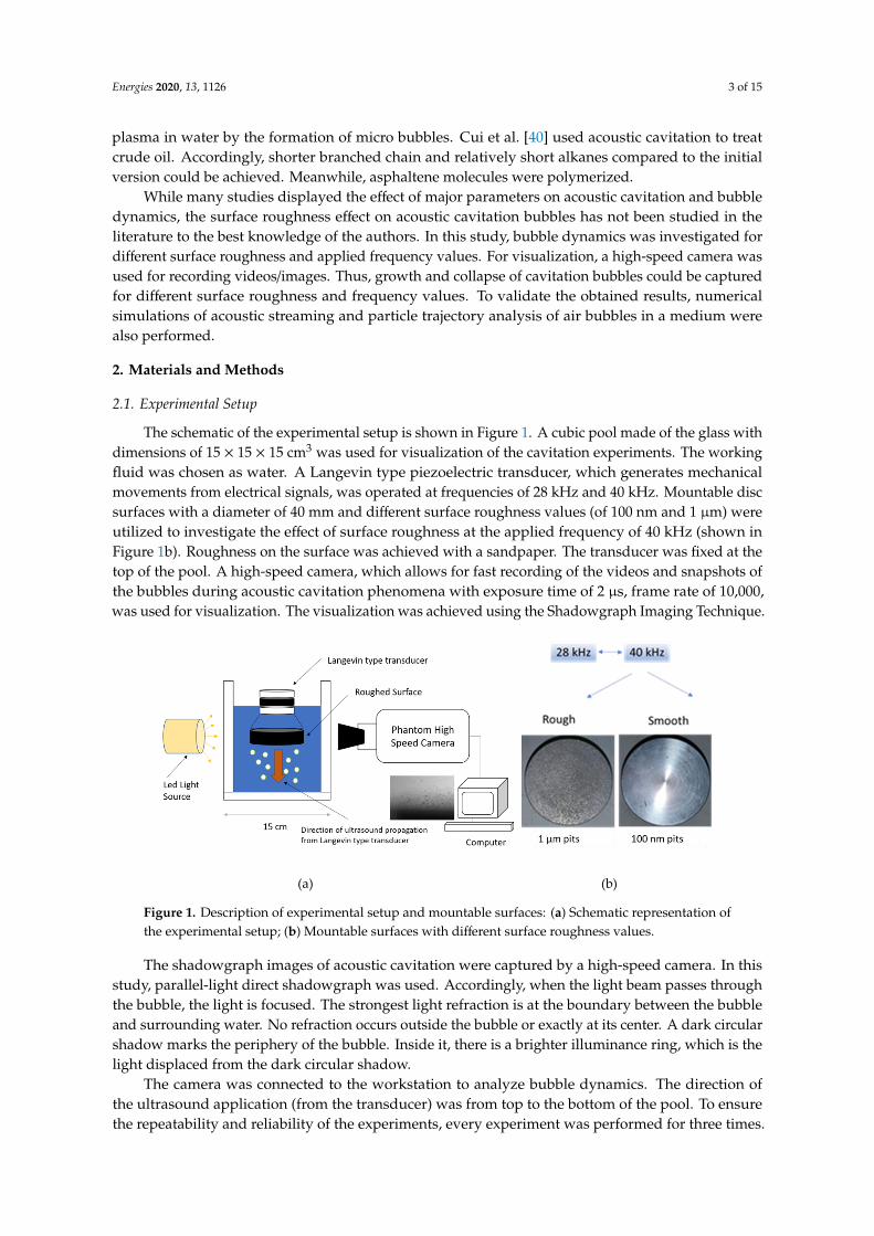
The sandwich-type transducers are used inside many industrial devices and are wellcharacterized [46,47]. The transducer usually has a single operating band, which has a fractionalbandwidth of around 5%. The operation frequency band was investigated using the experimentalsetup depicted in Figure 2a. A pulse generator (5072PR, Olympus CO. Waltham, MA, 02453, USA)excited the transducer using a wideband pulse, and the received echo was measured by a spectrumanalyzer (DSA875, Rigol, Beaverton, OR 97008, USA). The measure response showed a narrow bandcharacteristic with an operating frequency of 39.85 kHz (Figure 2b). The setup was used to determinethe exact operating frequency so that the transducer could be driven effectively.

Energies 2020, 13, 1126 4 of 14

Cavitation bubbles were generated using a sandwich-type ultrasonic transducer. The electronics

to drive this type of transducer mostly uses a digitally controlled push-pull transistor stage. To

prevent any short circuit, the transistor excitation timing is crucial for this type of design [41–45]. In

this study, a new driver circuit, which uses a simple function generator, was designed. The new

design simplifies electronics and reduces system complexity.

The sandwich-type transducers are used inside many industrial devices and are well

characterized [46,47]. The transducer usually has a single operating band, which has a fractional

bandwidth of around 5%. The operation frequency band was investigated using the experimental

setup depicted in Figure 2a. A pulse generator (5072PR, Olympus CO. Waltham, MA, 02453, USA)

excited the transducer using a wideband pulse, and the received echo was measured by a spectrum

analyzer (DSA875, Rigol, Beaverton, OR 97008, USA). The measure response showed a narrow band

characteristic with an operating frequency of 39.85 kHz (Figure 2b). The setup was used to determine

the exact operating frequency so that the transducer could be driven effectively.

(a) (b)

Figure 2. Characterization and measurement of transducer: (a) Transducer characterization setup;

(b) The measured frequency characteristics of a 40 kHz transducer.

The narrowband behavior of the transducer increased the dependency of efficiency on the

excitation frequency (e.g., 0.3% of the change in frequency would result in 20% of the change in the

power transmitted to the system). Hence the frequency stability had a significant effect on providing

constant power.

The designed driver circuitry was able to set the desired frequency and power level. The circuit

was controlled by a digital signal in order to provide frequency stability. Unlike the usual design, a

single switch was employed in the design. The high voltage switch pumped the electrical power to

the transducer by a predefined frequency. The switch was a metal-oxide semiconductor (MOS)

transistor connected to a high voltage direct current (HV-DC) supply, which was provided from

rectified alternating current (AC) voltage (220 V RMS). In the design, only a single switch was used.

It charged the piezoelectric transducer during on-time, and the accumulated charge was discharged

in off-time. The main component was inversely positioned fast diodes in the discharging circuitry.

Hence, only one switch was used to simplify the excitation circuit of the MOS transistor. A simple

function generator applied the pulse width modulated (PWM) signal to operate the system. The duty

cycle of the PWM signal defined the power (duty cycle must be under 40%), and the PWM frequency

determined the transducer’s operation point. The block schematic explaining the circuit design is

given in Figure 3a. The voltage across transducer nodes can be seen in Figure 3b, and the frequency

domain representation of the voltage shows that the transducer is actuated by a pretty narrow band

signal around the required frequency (Figure 3c).

Figure 2. Characterization and measurement of transducer: (a) Transducer characterization setup;(b) The measured frequency characteristics of a 40 kHz transducer.

The narrowband behavior of the transducer increased the dependency of efficiency on theexcitation frequency (e.g., 0.3% of the change in frequency would result in 20% of the change in thepower transmitted to the system). Hence the frequency stability had a significant effect on providingconstant power.

The designed driver circuitry was able to set the desired frequency and power level. The circuitwas controlled by a digital signal in order to provide frequency stability. Unlike the usual design,a single switch was employed in the design. The high voltage switch pumped the electrical powerto the transducer by a predefined frequency. The switch was a metal-oxide semiconductor (MOS)transistor connected to a high voltage direct current (HV-DC) supply, which was provided fromrectified alternating current (AC) voltage (220 V RMS). In the design, only a single switch was used.It charged the piezoelectric transducer during on-time, and the accumulated charge was dischargedin off-time. The main component was inversely positioned fast diodes in the discharging circuitry.Hence, only one switch was used to simplify the excitation circuit of the MOS transistor. A simplefunction generator applied the pulse width modulated (PWM) signal to operate the system. The dutycycle of the PWM signal defined the power (duty cycle must be under 40%), and the PWM frequencydetermined the transducer’s operation point. The block schematic explaining the circuit design is

Energies 2020, 13, 1126 5 of 15

given in Figure 3a. The voltage across transducer nodes can be seen in Figure 3b, and the frequencydomain representation of the voltage shows that the transducer is actuated by a pretty narrow bandsignal around the required frequency (Figure 3c).Energies 2020, 13, x FOR PEER REVIEW 5 of 15

(a)

(b) (c)

Figure 3. Schematic and characterization of utilized electronic circuit: (a) The block schematic of the

designed circuit; (b) Measured voltage when transducer is actuated by 26.7 kHz; (c) The frequency

domain representation of the voltage waveform given in (b).

2.3. Numerical Analysis

The COMSOL 5.4 software was used for solving the governing equations. Acoustic and particle

tracking modules were used to investigate the effect of acoustic field on air bubbles. Air bubbles were

considered as spherical particles with diameters ranging from 10µm to 50µm. Acoustophoretic

radiation, gravity and drag forces were implemented in the numerical domain. Open boundary

conditions were considered for side walls, while plane wave radiation was defined as the transducer

surface. The conservation equations for an acoustic wave propagation into a fluid are given as:

2

2 2

1 1. 0

PP

c t

(1)

Here, P, ρ, c, and t are pressure, density, sound velocity in medium (water), and time,

respectively. For a ( , ) ( ) i tP r t P r e solution, where , ,r r x y z is the position vector,

2 f is angular frequency, and f is the frequency. Substituting the pressure distribution into

Equation (1), the acoustic pressure ( )P r is obtained as:

2

2

10P P

c

(2)

The intensity distribution is expressed as:

Figure 3. Schematic and characterization of utilized electronic circuit: (a) The block schematic of thedesigned circuit; (b) Measured voltage when transducer is actuated by 26.7 kHz; (c) The frequencydomain representation of the voltage waveform given in (b).

2.3. Numerical Analysis

The COMSOL 5.4 software was used for solving the governing equations. Acoustic and particletracking modules were used to investigate the effect of acoustic field on air bubbles. Air bubbleswere considered as spherical particles with diameters ranging from 10 µm to 50 µm. Acoustophoreticradiation, gravity and drag forces were implemented in the numerical domain. Open boundaryconditions were considered for side walls, while plane wave radiation was defined as the transducersurface. The conservation equations for an acoustic wave propagation into a fluid are given as:

∇

(1ρ∇P

)−

1ρc2 .

∂2P∂t2 = 0 (1)

Here, P, %, c, and t are pressure, density, sound velocity in medium (water), and time, respectively.For a P(r, t) = P(r) · eiωt solution, where r = r(x, y, z) is the position vector, ω = 2π f is angularfrequency, and f is the frequency. Substituting the pressure distribution into Equation (1), the acousticpressure P(r) is obtained as:

∇

(1ρ∇P

)−ω2

ρc2 P = 0 (2)

Energies 2020, 13, 1126 6 of 15

The intensity distribution is expressed as:

I(r) =p(r)2

2ρc(3)

After mesh dependency analysis, the homogeneous pressure equation was solved as:

P(r, t) = Aei(ωt−kr) (4)

3. Results and Discussion

3.1. Single Bubble Dynamics in an Acoustic Field

When appropriate ultrasonic radiation is applied, “multi-bubbles” appear in a liquid medium.The generated bubbles can be formed due to either the existence of the dissolved gas nuclei or thecaged gases in the solid particles. Another reason for the formation of bubbles can be attributed to theseparation of larger bubbles in the liquid medium. Theoretically, if the bubble overcomes the pressurethreshold, which is called the Blake threshold, PB, (Equation (5)), nucleation takes place [1]:

PB = P0 +8σ9

√√√√ 3σ

2[P0 + (2σ/RB)R3

B

] (5)

where P0, RB and σ are the ambient pressure, Blake radius and surface tension, respectively.Upon nucleation, the bubble can start to grow and go through stable cavitation for a large drivingacoustic pressure. On the other hand, if the driving acoustic pressure is low, the bubbles dissolve inthe medium. For much higher acoustic pressures, which exceed the cavitation threshold, the bubblesbecome unstable or transient. In another scenario, larger bubbles can be affected by the buoyancy forceand move up to the surface of the liquid medium, which is referred as “degassing”.

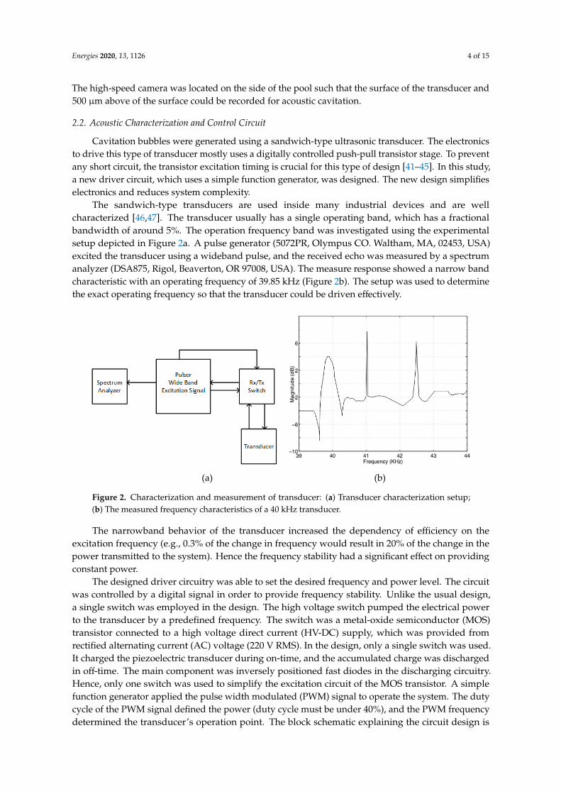
The bubble growth process at an applied ultrasonic frequency is mainly separated into twodifferent mechanisms: rectified diffusion and coalescence. The coalescence occurs due to the secondaryBjerknes force [48] between two oscillating bubbles in the same oscillation phase. They merge and forma bigger bubble. The growth of the bubbles via the coalescence mechanism is faster than the rectifieddiffusion. Figure 4 represents the rectified diffusion, in which the sinusoidal acoustic streaming affectsthe bubble dynamics and causes periodical growth and wane. During the growth, the expansion takesplace, the inner pressure of the bubble is low, and the diffusion of gas into the bubble occurs. Inversely,the diffusion of the gas out of the bubble appears at the time of compression. After the bubble reachesthe critical maximum size, the bubble collapse occurs which leads to pressure shockwaves.

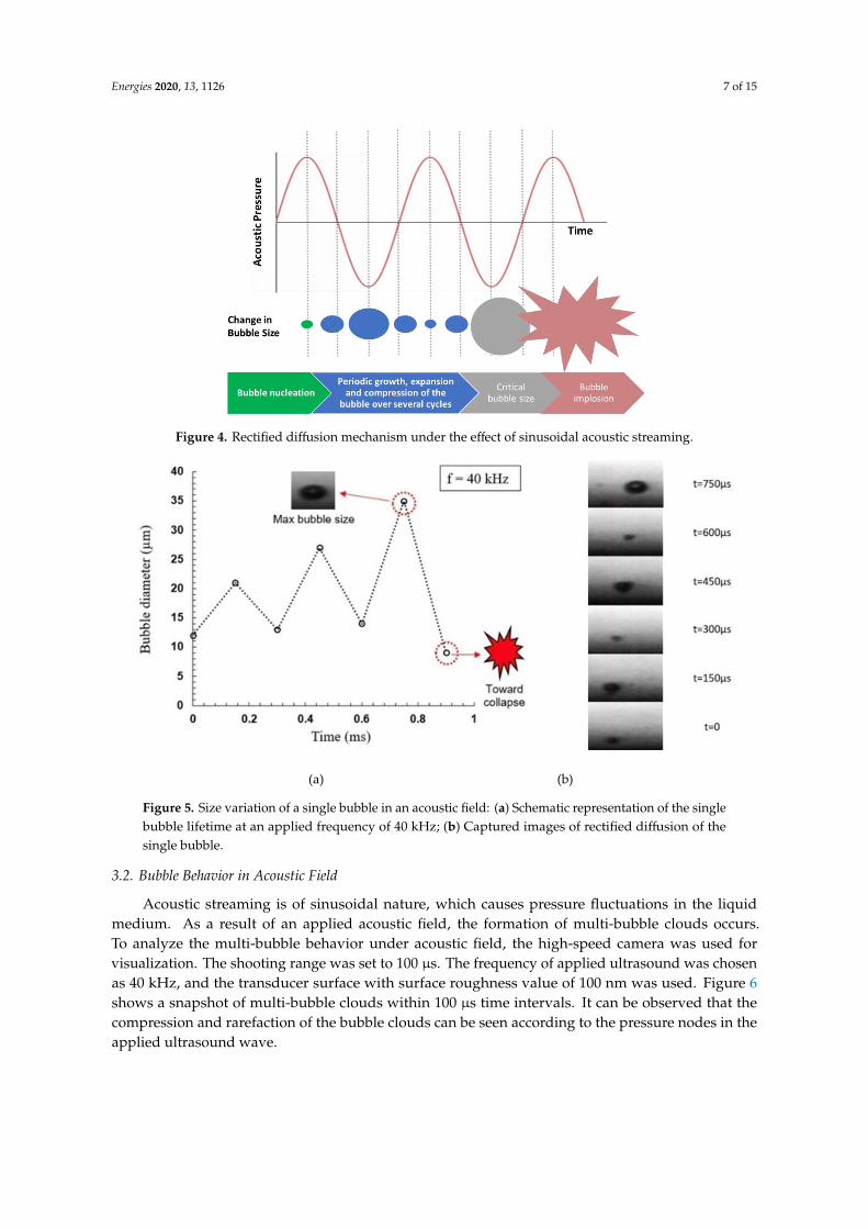
An example of a single bubble lifetime at the applied 40 kHz acoustic field frequency is shownin Figure 5a. The experiment is conducted with a smooth transducer surface. By using fast videorecording, the rectified diffusion of the single bubble was recorded in every 150 µs, as shown inFigure 5b. The bubble goes through the rectified diffusion, and its size alters according to the insidepressure. The pressure difference between the liquid medium and the inner bubble allows for theperiodic growth, expansion and compression of the bubble over several cycles. After 750 µs, the bubblereaches the maximum size, which is found as approximately 35 µm, which is followed by the violentcollapse of the bubble.

Energies 2020, 13, 1126 7 of 15

Energies 2020, 13, x FOR PEER REVIEW 6 of 15

2( )( )

2

p rI r

c (3)

After mesh dependency analysis, the homogeneous pressure equation was solved as:

( )( , ) i t krP r t Ae (4)

3. Results and Discussion

3.1. Single Bubble Dynamics in an Acoustic Field

When appropriate ultrasonic radiation is applied, “multi-bubbles” appear in a liquid medium.

The generated bubbles can be formed due to either the existence of the dissolved gas nuclei or the

caged gases in the solid particles. Another reason for the formation of bubbles can be attributed to

the separation of larger bubbles in the liquid medium. Theoretically, if the bubble overcomes the

pressure threshold, which is called the Blake threshold, PB, (Equation (5)), nucleation takes place [1]:

0 3

0

8 3

9 2 2B

B B

P PP R R

(5)

where P0, RB and σ are the ambient pressure, Blake radius and surface tension, respectively. Upon

nucleation, the bubble can start to grow and go through stable cavitation for a large driving acoustic

pressure. On the other hand, if the driving acoustic pressure is low, the bubbles dissolve in the

medium. For much higher acoustic pressures, which exceed the cavitation threshold, the bubbles

become unstable or transient. In another scenario, larger bubbles can be affected by the buoyancy

force and move up to the surface of the liquid medium, which is referred as “degassing”.

The bubble growth process at an applied ultrasonic frequency is mainly separated into two

different mechanisms: rectified diffusion and coalescence. The coalescence occurs due to the

secondary Bjerknes force [48] between two oscillating bubbles in the same oscillation phase. They

merge and form a bigger bubble. The growth of the bubbles via the coalescence mechanism is faster

than the rectified diffusion. Figure 4 represents the rectified diffusion, in which the sinusoidal

acoustic streaming affects the bubble dynamics and causes periodical growth and wane. During the

growth, the expansion takes place, the inner pressure of the bubble is low, and the diffusion of gas

into the bubble occurs. Inversely, the diffusion of the gas out of the bubble appears at the time of

compression. After the bubble reaches the critical maximum size, the bubble collapse occurs which

leads to pressure shockwaves.

Figure 4. Rectified diffusion mechanism under the effect of sinusoidal acoustic streaming. Figure 4. Rectified diffusion mechanism under the effect of sinusoidal acoustic streaming.

Energies 2020, 13, x FOR PEER REVIEW 7 of 15

An example of a single bubble lifetime at the applied 40 kHz acoustic field frequency is shown

in Figure 5a. The experiment is conducted with a smooth transducer surface. By using fast video

recording, the rectified diffusion of the single bubble was recorded in every 150 µs, as shown in

Figure 5b. The bubble goes through the rectified diffusion, and its size alters according to the inside

pressure. The pressure difference between the liquid medium and the inner bubble allows for the

periodic growth, expansion and compression of the bubble over several cycles. After 750 µs, the

bubble reaches the maximum size, which is found as approximately 35 µm, which is followed by the

violent collapse of the bubble.

(a) (b)

Figure 5. Size variation of a single bubble in an acoustic field: (a) Schematic representation of the

single bubble lifetime at an applied frequency of 40 kHz; (b) Captured images of rectified diffusion of

the single bubble

3.2. Bubble Behavior in Acoustic Field

Acoustic streaming is of sinusoidal nature, which causes pressure fluctuations in the liquid

medium. As a result of an applied acoustic field, the formation of multi-bubble clouds occurs. To

analyze the multi-bubble behavior under acoustic field, the high-speed camera was used for

visualization. The shooting range was set to 100 µs. The frequency of applied ultrasound was chosen

as 40 kHz, and the transducer surface with surface roughness value of 100 nm was used. Figure 6

shows a snapshot of multi-bubble clouds within 100 µs time intervals. It can be observed that the

compression and rarefaction of the bubble clouds can be seen according to the pressure nodes in the

applied ultrasound wave.

Figure 5. Size variation of a single bubble in an acoustic field: (a) Schematic representation of the singlebubble lifetime at an applied frequency of 40 kHz; (b) Captured images of rectified diffusion of thesingle bubble.

3.2. Bubble Behavior in Acoustic Field

Acoustic streaming is of sinusoidal nature, which causes pressure fluctuations in the liquidmedium. As a result of an applied acoustic field, the formation of multi-bubble clouds occurs.To analyze the multi-bubble behavior under acoustic field, the high-speed camera was used forvisualization. The shooting range was set to 100 µs. The frequency of applied ultrasound was chosenas 40 kHz, and the transducer surface with surface roughness value of 100 nm was used. Figure 6shows a snapshot of multi-bubble clouds within 100 µs time intervals. It can be observed that thecompression and rarefaction of the bubble clouds can be seen according to the pressure nodes in theapplied ultrasound wave.

Energies 2020, 13, 1126 8 of 15

Energies 2020, 13, 1126 7 of 14

(a) (b)

Figure 5. Size variation of a single bubble in an acoustic field: (a) Schematic representation of the

single bubble lifetime at an applied frequency of 40 kHz; (b) Captured images of rectified diffusion of

the single bubble

3.2. Bubble Behavior in Acoustic Field

Acoustic streaming is of sinusoidal nature, which causes pressure fluctuations in the liquid

medium. As a result of an applied acoustic field, the formation of multi-bubble clouds occurs. To

analyze the multi-bubble behavior under acoustic field, the high-speed camera was used for

visualization. The shooting range was set to 100 µs. The frequency of applied ultrasound was chosen

as 40 kHz, and the transducer surface with surface roughness value of 100 nm was used. Figure 6

shows a snapshot of multi-bubble clouds within 100 µs time intervals. It can be observed that the

compression and rarefaction of the bubble clouds can be seen according to the pressure nodes in the

applied ultrasound wave.

Figure 6. Cont.

Energies 2020, 13, 1126 8 of 14

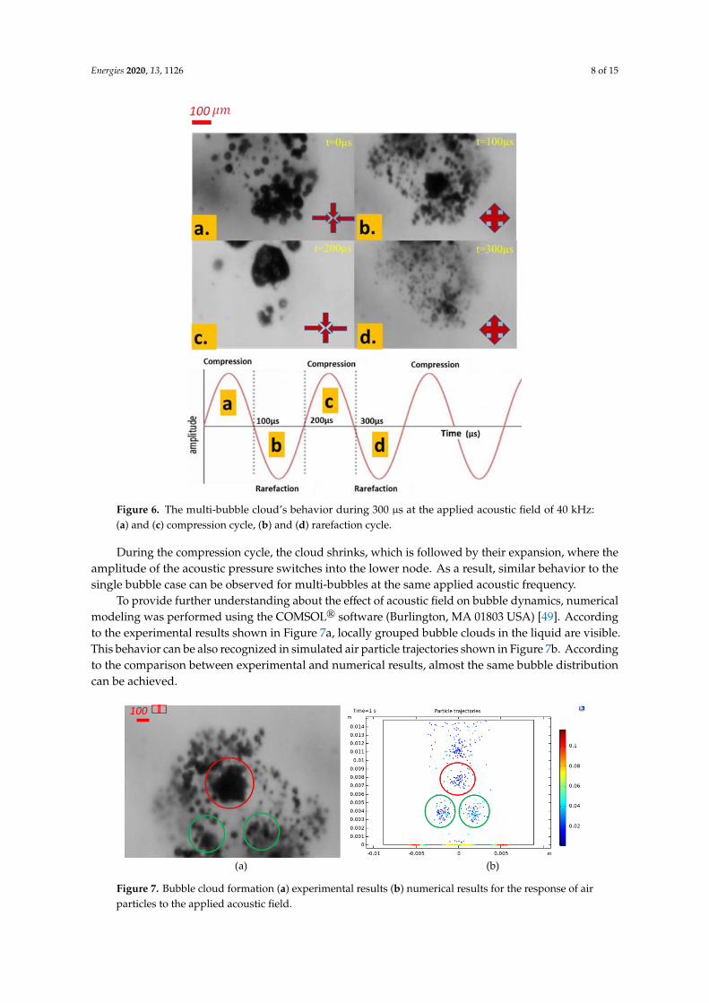
Figure 6. The multi-bubble cloud’s behavior during 300 µs at the applied acoustic field of 40 kHz: (a)

and (c) compression cycle, (b) and (d) rarefaction cycle.

During the compression cycle, the cloud shrinks, which is followed by their expansion, where

the amplitude of the acoustic pressure switches into the lower node. As a result, similar behavior to

the single bubble case can be observed for multi-bubbles at the same applied acoustic frequency.

To provide further understanding about the effect of acoustic field on bubble dynamics,

numerical modeling was performed using the COMSOL® software (Burlington, MA 01803 USA) [49].

According to the experimental results shown in Figure 7a, locally grouped bubble clouds in the liquid

are visible. This behavior can be also recognized in simulated air particle trajectories shown in Figure

7b. According to the comparison between experimental and numerical results, almost the same

bubble distribution can be achieved.

(a) (b)

Figure 7. Bubble cloud formation (a) experimental results (b) numerical results for the response of

air particles to the applied acoustic field.

An oscillating flow field can be described as an acoustic wave with infinite wavelength. The flow

velocity is expressed as ˆ( ) sinc c fu t u t , where ˆcu is the amplitude of the velocity wave and

2f rf is the angular frequency. Resonance size, Stokes number, t rS f c , and density ratio,

p l , are major parameters affecting the response of air particles to the acoustic field.

The acting radiation force on the bubbles inside the medium is due pressure gradient expressed

asP Du

x Dt

. In addition to the primary radiation force, which acts in the direction of acoustic

wave propagation, a secondary radiation force manipulates the agents to attract or repel each other.

The time-dependent radiation force on the bubble can be calculated from the driving pressure wave

and time-dependent volume of the bubble. Furthermore, the translational motion of the bubble in

response to the radiation force can be calculated by solving the equations of air particle trajectory.

100� �

Figure 6. The multi-bubble cloud’s behavior during 300 µs at the applied acoustic field of 40 kHz:(a) and (c) compression cycle, (b) and (d) rarefaction cycle.

During the compression cycle, the cloud shrinks, which is followed by their expansion, where theamplitude of the acoustic pressure switches into the lower node. As a result, similar behavior to thesingle bubble case can be observed for multi-bubbles at the same applied acoustic frequency.

To provide further understanding about the effect of acoustic field on bubble dynamics, numericalmodeling was performed using the COMSOL® software (Burlington, MA 01803 USA) [49]. Accordingto the experimental results shown in Figure 7a, locally grouped bubble clouds in the liquid are visible.This behavior can be also recognized in simulated air particle trajectories shown in Figure 7b. Accordingto the comparison between experimental and numerical results, almost the same bubble distributioncan be achieved.

Energies 2020, 13, 1126 8 of 15

Figure 6. Cont.

Figure 6. The multi-bubble cloud’s behavior during 300 µs at the applied acoustic field of 40 kHz: (a) and (c) compression cycle, (b) and (d) rarefaction cycle.

During the compression cycle, the cloud shrinks, which is followed by their expansion, where the amplitude of the acoustic pressure switches into the lower node. As a result, similar behavior to the single bubble case can be observed for multi-bubbles at the same applied acoustic frequency.

To provide further understanding about the effect of acoustic field on bubble dynamics, numerical modeling was performed using the COMSOL® software (Burlington, MA 01803 USA) [49]. According to the experimental results shown in Figure 7a, locally grouped bubble clouds in the liquid are visible. This behavior can be also recognized in simulated air particle trajectories shown in Figure 7b. According to the comparison between experimental and numerical results, almost the same bubble distribution can be achieved.

(a) (b)

100 ��

Figure 7. Bubble cloud formation (a) experimental results (b) numerical results for the response of airparticles to the applied acoustic field.

Energies 2020, 13, 1126 9 of 15

An oscillating flow field can be described as an acoustic wave with infinite wavelength. The flowvelocity is expressed as uc(t) = uc sin

(ω f t

), where uc is the amplitude of the velocity wave and

ω f = 2π fr is the angular frequency. Resonance size, Stokes number, St = fr/c, and density ratio,γ = ρp/ρl, are major parameters affecting the response of air particles to the acoustic field.

The acting radiation force on the bubbles inside the medium is due pressure gradient expressedas ∂P

∂x = −ρDuDt . In addition to the primary radiation force, which acts in the direction of acoustic

wave propagation, a secondary radiation force manipulates the agents to attract or repel each other.The time-dependent radiation force on the bubble can be calculated from the driving pressure wave andtime-dependent volume of the bubble. Furthermore, the translational motion of the bubble in responseto the radiation force can be calculated by solving the equations of air particle trajectory. For an airparticle with mass of mb = ρVb, the particle trajectory equation is given as mb

dubdt = FR(t) + FQS(t).

The radiation force (FR(t)) and quasi-static drag force (FQS(t)) are expressed as:

FR(t) = −VbdPdriv

dx(6)

FQS(t) =12ρl|ur|urA

242R|ul−ub|

υ

(1 + 0.197

(2R|ul − ub|

0.63

υ

))(7)

Here, mb is the air particle mass, ub is the air particle velocity, dPdriv is the driving pressuredifference, u is the velocity, ur = ul − ub is the relative velocity, and υ is the viscosity. To examine theeffect of radiation force, the motion of bubbles with different diameters was simulated at the 40 kHzultrasonic frequency. The obtained results are shown in Figure 8. Accordingly, the bubbles withdiameters smaller than 10 µm are not affected by the acoustic field, while bubbles with diameters largerthan 50 µm can be sorted according to the radiation potential map. The obtained results indicate thatthe response of air particles to the radiation force is proportional to their size, which is also displayedby the visual images shown in Figure 7a.

Energies 2020, 13, x FOR PEER REVIEW 9 of 15

(a) (b)

Figure 7. Bubble cloud formation (a) experimental results (b) numerical results for the response of

air particles to the applied acoustic field.

An oscillating flow field can be described as an acoustic wave with infinite wavelength. The flow

velocity is expressed as ˆ( ) sinc c fu t u t , where ˆcu is the amplitude of the velocity wave and

2f rf is the angular frequency. Resonance size, Stokes number, t rS f c , and density ratio,

p l , are major parameters affecting the response of air particles to the acoustic field.

The acting radiation force on the bubbles inside the medium is due pressure gradient expressed

asP Du

x Dt

. In addition to the primary radiation force, which acts in the direction of acoustic

wave propagation, a secondary radiation force manipulates the agents to attract or repel each other.

The time-dependent radiation force on the bubble can be calculated from the driving pressure wave

and time-dependent volume of the bubble. Furthermore, the translational motion of the bubble in

response to the radiation force can be calculated by solving the equations of air particle trajectory.

For an air particle with mass of 𝑚𝑏 = 𝜌𝑉𝑏 , the particle trajectory equation is given as 𝑚𝑏𝑑𝑢𝑏

𝑑𝑡=

𝐹𝑅(𝑡) + 𝐹𝑄𝑆(𝑡). The radiation force (𝐹𝑅(𝑡)) and quasi-static drag force (𝐹𝑄𝑆(𝑡)) are expressed as:

𝐹𝑅(𝑡) = −𝑉𝑏𝑑𝑃𝑑𝑟𝑖𝑣

𝑑𝑥⁄ (6)

𝐹𝑄𝑆(𝑡) =1

2𝜌𝑙|𝑢𝑟|𝑢𝑟𝐴

24

2𝑅|𝑢𝑙 − 𝑢𝑏|𝜐

(1 + 0.197 (2𝑅|𝑢𝑙 − 𝑢𝑏|0.63

𝜐)) (7)

Here, 𝑚𝑏 is the air particle mass, 𝑢𝑏 is the air particle velocity, 𝑑𝑃𝑑𝑟𝑖𝑣 is the driving pressure

difference, 𝑢 is the velocity, 𝑢𝑟 = 𝑢𝑙 − 𝑢𝑏 is the relative velocity, and 𝜐 is the viscosity. To examine

the effect of radiation force, the motion of bubbles with different diameters was simulated at the 40

kHz ultrasonic frequency. The obtained results are shown in Figure 8. Accordingly, the bubbles with

diameters smaller than 10 µm are not affected by the acoustic field, while bubbles with diameters

larger than 50 µm can be sorted according to the radiation potential map. The obtained results

indicate that the response of air particles to the radiation force is proportional to their size, which is

also displayed by the visual images shown in Figure 7a.

(a) (b)

Figure 8. Simulation results of bubble trajectories with the bubbles having different sizes at the

applied frequency of 40 kHz (a) Air bubble having 50 µm diameter; (b) Air bubble having 10 µm

diameter.

3.3. Effect of Surface Roughness and Ultrasonic Frequency

Figure 9 shows the acoustic cavitation induced bubbles at the applied ultrasonic frequency of 40

kHz when different surfaces are mounted on the transducer. The images were taken with the high-

Figure 8. Simulation results of bubble trajectories with the bubbles having different sizes at the appliedfrequency of 40 kHz (a) Air bubble having 50 µm diameter; (b) Air bubble having 10 µm diameter.

3.3. Effect of Surface Roughness and Ultrasonic Frequency

Figure 9 shows the acoustic cavitation induced bubbles at the applied ultrasonic frequency of40 kHz when different surfaces are mounted on the transducer. The images were taken with thehigh-speed camera and 100 µs time slots. Figure 9a displays the multi-bubble formation when thesmooth surface (with 100 nm surface roughness) is tested. The bubbles appear and form a cloud.Meantime, the bubbles on the rough surface exhibit more disorganized behavior. As a result, the cavitylength diminution is evident with the increase in the roughness.

Energies 2020, 13, 1126 10 of 15

When a single acoustic cavitation bubble collapses in the liquid medium, the temperature can belocally increased up to 10,000 K [1]. The pool temperatures were measured at four different locations.The average temperature of four thermocouples were recorded for analysis purposes. The experimentswere conducted under the 40 kHz applied ultrasonic field.

Energies 2020, 13, x FOR PEER REVIEW 10 of 15

speed camera and 100 µs time slots. Figure 9a displays the multi-bubble formation when the smooth

surface (with 100 nm surface roughness) is tested. The bubbles appear and form a cloud. Meantime,

the bubbles on the rough surface exhibit more disorganized behavior. As a result, the cavity length

diminution is evident with the increase in the roughness.

When a single acoustic cavitation bubble collapses in the liquid medium, the temperature can

be locally increased up to 10,000 K [1]. The pool temperatures were measured at four different

locations. The average temperature of four thermocouples were recorded for analysis purposes. The

experiments were conducted under the 40 kHz applied ultrasonic field.

(a) (b)

Figure 9. The cavitation bubbles at 40 kHz. (a) Multi-bubble cloud formation on a smooth surface

with 100 nm roughness; (b) Disorganized bubbles with diminution of cavity length on a rough surface

with 1 µm roughness.

The temperature variations of the pool with time are shown in Figure 10. Accordingly, for

surface roughness of 100 nm, the temperature increases from 299 K (room temperature) to 340 K after

35 minutes of experimentation. The reason for the temperature rise can be the energy released during

the bubble collapse. On the other hand, for the surface with surface roughness parameter Ra=1 µm,

the pool temperature is stabilized within a shorter time (almost 25 minutes). Here, Here, Ra is the

arithmetical mean deviation of the assessed profile and is calculated as 𝑅𝑎 =1

𝑛∑ |𝑦𝑖|𝑛

𝑖=1 , where, yi is

the vertical distance from the mean line to the ith data point. Moreover, the pool temperature is 10 K

colder than the previous case (smooth surface), which is due to lower intensity of cavitation inside

the pool for the case of rough surface.

Figure 10. The temperature rise during the acoustic cavitation experiments at the applied frequency

of 40 kHz.

Figure 9. The cavitation bubbles at 40 kHz. (a) Multi-bubble cloud formation on a smooth surface with100 nm roughness; (b) Disorganized bubbles with diminution of cavity length on a rough surface with1 µm roughness.

The temperature variations of the pool with time are shown in Figure 10. Accordingly, for surfaceroughness of 100 nm, the temperature increases from 299 K (room temperature) to 340 K after 35minutes of experimentation. The reason for the temperature rise can be the energy released duringthe bubble collapse. On the other hand, for the surface with surface roughness parameter Ra = 1 µm,the pool temperature is stabilized within a shorter time (almost 25 minutes). Here, Here, Ra is thearithmetical mean deviation of the assessed profile and is calculated as Ra = 1

n∑n

i=1

∣∣∣yi∣∣∣, where, yi is

the vertical distance from the mean line to the ith data point. Moreover, the pool temperature is 10 Kcolder than the previous case (smooth surface), which is due to lower intensity of cavitation inside thepool for the case of rough surface.

Energies 2020, 13, x FOR PEER REVIEW 10 of 15

speed camera and 100 µs time slots. Figure 9a displays the multi-bubble formation when the smooth

surface (with 100 nm surface roughness) is tested. The bubbles appear and form a cloud. Meantime,

the bubbles on the rough surface exhibit more disorganized behavior. As a result, the cavity length

diminution is evident with the increase in the roughness.

When a single acoustic cavitation bubble collapses in the liquid medium, the temperature can

be locally increased up to 10,000 K [1]. The pool temperatures were measured at four different

locations. The average temperature of four thermocouples were recorded for analysis purposes. The

experiments were conducted under the 40 kHz applied ultrasonic field.

(a) (b)

Figure 9. The cavitation bubbles at 40 kHz. (a) Multi-bubble cloud formation on a smooth surface

with 100 nm roughness; (b) Disorganized bubbles with diminution of cavity length on a rough surface

with 1 µm roughness.

The temperature variations of the pool with time are shown in Figure 10. Accordingly, for

surface roughness of 100 nm, the temperature increases from 299 K (room temperature) to 340 K after

35 minutes of experimentation. The reason for the temperature rise can be the energy released during

the bubble collapse. On the other hand, for the surface with surface roughness parameter Ra=1 µm,

the pool temperature is stabilized within a shorter time (almost 25 minutes). Here, Here, Ra is the

arithmetical mean deviation of the assessed profile and is calculated as 𝑅𝑎 =1

𝑛∑ |𝑦𝑖|𝑛

𝑖=1 , where, yi is

the vertical distance from the mean line to the ith data point. Moreover, the pool temperature is 10 K

colder than the previous case (smooth surface), which is due to lower intensity of cavitation inside

the pool for the case of rough surface.

Figure 10. The temperature rise during the acoustic cavitation experiments at the applied frequency

of 40 kHz.

Figure 10. The temperature rise during the acoustic cavitation experiments at the applied frequency of40 kHz.

Energies 2020, 13, 1126 11 of 15

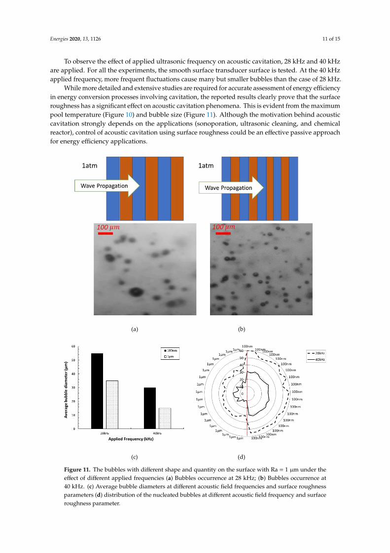
To observe the effect of applied ultrasonic frequency on acoustic cavitation, 28 kHz and 40 kHzare applied. For all the experiments, the smooth surface transducer surface is tested. At the 40 kHzapplied frequency, more frequent fluctuations cause many but smaller bubbles than the case of 28 kHz.

While more detailed and extensive studies are required for accurate assessment of energy efficiencyin energy conversion processes involving cavitation, the reported results clearly prove that the surfaceroughness has a significant effect on acoustic cavitation phenomena. This is evident from the maximumpool temperature (Figure 10) and bubble size (Figure 11). Although the motivation behind acousticcavitation strongly depends on the applications (sonoporation, ultrasonic cleaning, and chemicalreactor), control of acoustic cavitation using surface roughness could be an effective passive approachfor energy efficiency applications.

Energies 2020, 13, x FOR PEER REVIEW 11 of 15

To observe the effect of applied ultrasonic frequency on acoustic cavitation, 28 kHz and 40 kHz

are applied. For all the experiments, the smooth surface transducer surface is tested. At the 40 kHz

applied frequency, more frequent fluctuations cause many but smaller bubbles than the case of 28

kHz.

While more detailed and extensive studies are required for accurate assessment of energy

efficiency in energy conversion processes involving cavitation, the reported results clearly prove that

the surface roughness has a significant effect on acoustic cavitation phenomena. This is evident from

the maximum pool temperature (Figure 10) and bubble size (Figure 11). Although the motivation

behind acoustic cavitation strongly depends on the applications (sonoporation, ultrasonic cleaning,

and chemical reactor), control of acoustic cavitation using surface roughness could be an effective

passive approach for energy efficiency applications.

(a) (b)

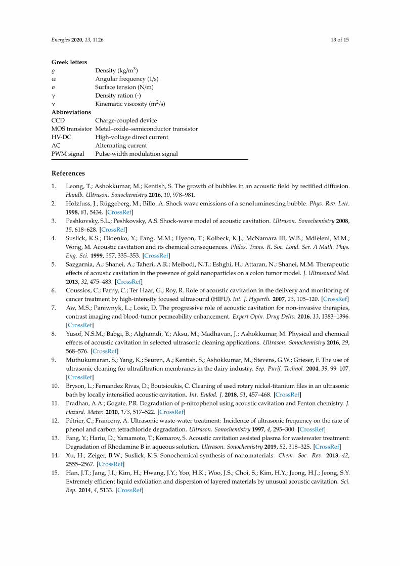
(c) (d)

Figure 11. The bubbles with different shape and quantity on the surface with Ra=1µm under the effect

of different applied frequencies (a) Bubbles occurrence at 28 kHz; (b) Bubbles occurrence at 40 kHz.

(c) Average bubble diameters at different acoustic field frequencies and surface roughness parameters

(d) distribution of the nucleated bubbles at different acoustic field frequency and surface roughness

parameter.

Figure 11. The bubbles with different shape and quantity on the surface with Ra = 1 µm under theeffect of different applied frequencies (a) Bubbles occurrence at 28 kHz; (b) Bubbles occurrence at40 kHz. (c) Average bubble diameters at different acoustic field frequencies and surface roughnessparameters (d) distribution of the nucleated bubbles at different acoustic field frequency and surfaceroughness parameter.

Energies 2020, 13, 1126 12 of 15

As seen in Figure 11a, there are approximately 20 bubbles, whereas 50 bubbles are visible on thesame scale in Figure 11b. The average size of generated bubbles under the 40 kHz acoustic field isalmost twice as much as the size of generated bubbles under the 28 kHz acoustic field. As the size ofbubbles increases, the generated energy due to bubble collapse remarkably decreases. Furthermore,as can be seen in Figure 11c, surface roughness reduces the bubble size. The main reason is thepropagation angle of surface acoustic wave propagation. As surface roughness increases, surface wavepropagation occurs with lower velocity, and scattering increases, thereby weakening the wave.

4. Conclusions

This study was performed to provide more information about the effect of surface on acousticcavitation at two widely used applied ultrasonic frequencies below 50 kHz. The investigation ofthe effect of surface within this range is critical for many applications such as ultrasonic cleaningand drug delivery. The effect of surface roughness on bubble dynamics in acoustic cavitation wasexperimentally and numerically investigated. Surfaces with roughness values of 100 nm and 1 µmwere examined in the 28 kHz and 48 kHz acoustic fields. DI-water was used as the working fluid.A high-speed camera was used to capture bubble dynamics inside the pool. Single bubble lifetime wasinvestigated based on visual results. The average bubble sizes for different conditions were obtainedand tabulated. It was found that surface roughness reduced the bubble size. The numerical analysisindicated that the bubbles with diameters smaller than 10 µm were not affected by the acoustic field,while bubbles with a diameter of 50 µm could be sorted according to the radiation potential map.The obtained results showed that the response of air bubbles to the radiation force was proportionalto their size. The recorded pool temperatures revealed that the pool temperature was stabilizedwithin a shorter time (almost 10 minutes shorter) for the surface with Ra = 1 µm. Moreover, the pooltemperature was 10 K colder than the previous case (smooth surface), which was due to lower intensityof cavitation inside the pool for the case of rough surface. More studies are required in this field todeepen the understanding about the effect of surface on plane wave propagation and subsequentacoustic cavitation within the medium.

Author Contributions: Conceptualization, Methodology, Validation: R.A. and A.K.S.; Software, Setup preparation:M.I.S.; Acoustic Circuit Design: A.S.; Supervision: A.K. All authors have read and agreed to the published versionof the manuscript.

Funding: This research received no external funding.

Acknowledgments: The equipment and characterization support provided by the Sabanci UniversityNanotechnology Research and Applications Center (SUNUM) and its staff members are appreciated.

Conflicts of Interest: The authors declare no conflict of interest.

Nomenclature

Parameter Descriptionc Sound velocity (m/s)f Frequency (1/s)FR Radiation force (N)FQS Quasi-static drag force (N)k Wave number (1/m)P Pressure (kPa)P0 Ambient pressure (kPa)R Bubble radius (m)St Stokes number (-)t Time (s)u(t) Velocity (m/s)ur Relative velocity (m/s)V Velocity (m/s)

Energies 2020, 13, 1126 13 of 15

Greek letters% Density (kg/m3)ω Angular frequency (1/s)σ Surface tension (N/m)γ Density ration (-)ν Kinematic viscosity (m2/s)AbbreviationsCCD Charge-coupled deviceMOS transistor Metal–oxide–semiconductor transistorHV-DC High-voltage direct currentAC Alternating currentPWM signal Pulse-width modulation signal

References

1. Leong, T.; Ashokkumar, M.; Kentish, S. The growth of bubbles in an acoustic field by rectified diffusion.Handb. Ultrason. Sonochemistry 2016, 10, 978–981.

2. Holzfuss, J.; Rüggeberg, M.; Billo, A. Shock wave emissions of a sonoluminescing bubble. Phys. Rev. Lett.1998, 81, 5434. [CrossRef]

3. Peshkovsky, S.L.; Peshkovsky, A.S. Shock-wave model of acoustic cavitation. Ultrason. Sonochemistry 2008,15, 618–628. [CrossRef]

4. Suslick, K.S.; Didenko, Y.; Fang, M.M.; Hyeon, T.; Kolbeck, K.J.; McNamara III, W.B.; Mdleleni, M.M.;Wong, M. Acoustic cavitation and its chemical consequences. Philos. Trans. R. Soc. Lond. Ser. A Math. Phys.Eng. Sci. 1999, 357, 335–353. [CrossRef]

5. Sazgarnia, A.; Shanei, A.; Taheri, A.R.; Meibodi, N.T.; Eshghi, H.; Attaran, N.; Shanei, M.M. Therapeuticeffects of acoustic cavitation in the presence of gold nanoparticles on a colon tumor model. J. Ultrasound Med.2013, 32, 475–483. [CrossRef]

6. Coussios, C.; Farny, C.; Ter Haar, G.; Roy, R. Role of acoustic cavitation in the delivery and monitoring ofcancer treatment by high-intensity focused ultrasound (HIFU). Int. J. Hyperth. 2007, 23, 105–120. [CrossRef]

7. Aw, M.S.; Paniwnyk, L.; Losic, D. The progressive role of acoustic cavitation for non-invasive therapies,contrast imaging and blood-tumor permeability enhancement. Expert Opin. Drug Deliv. 2016, 13, 1383–1396.[CrossRef]

8. Yusof, N.S.M.; Babgi, B.; Alghamdi, Y.; Aksu, M.; Madhavan, J.; Ashokkumar, M. Physical and chemicaleffects of acoustic cavitation in selected ultrasonic cleaning applications. Ultrason. Sonochemistry 2016, 29,568–576. [CrossRef]

9. Muthukumaran, S.; Yang, K.; Seuren, A.; Kentish, S.; Ashokkumar, M.; Stevens, G.W.; Grieser, F. The use ofultrasonic cleaning for ultrafiltration membranes in the dairy industry. Sep. Purif. Technol. 2004, 39, 99–107.[CrossRef]

10. Bryson, L.; Fernandez Rivas, D.; Boutsioukis, C. Cleaning of used rotary nickel-titanium files in an ultrasonicbath by locally intensified acoustic cavitation. Int. Endod. J. 2018, 51, 457–468. [CrossRef]

11. Pradhan, A.A.; Gogate, P.R. Degradation of p-nitrophenol using acoustic cavitation and Fenton chemistry. J.Hazard. Mater. 2010, 173, 517–522. [CrossRef]

12. Pétrier, C.; Francony, A. Ultrasonic waste-water treatment: Incidence of ultrasonic frequency on the rate ofphenol and carbon tetrachloride degradation. Ultrason. Sonochemistry 1997, 4, 295–300. [CrossRef]

13. Fang, Y.; Hariu, D.; Yamamoto, T.; Komarov, S. Acoustic cavitation assisted plasma for wastewater treatment:Degradation of Rhodamine B in aqueous solution. Ultrason. Sonochemistry 2019, 52, 318–325. [CrossRef]

14. Xu, H.; Zeiger, B.W.; Suslick, K.S. Sonochemical synthesis of nanomaterials. Chem. Soc. Rev. 2013, 42,2555–2567. [CrossRef]

15. Han, J.T.; Jang, J.I.; Kim, H.; Hwang, J.Y.; Yoo, H.K.; Woo, J.S.; Choi, S.; Kim, H.Y.; Jeong, H.J.; Jeong, S.Y.Extremely efficient liquid exfoliation and dispersion of layered materials by unusual acoustic cavitation. Sci.Rep. 2014, 4, 5133. [CrossRef]

Energies 2020, 13, 1126 14 of 15

16. Hockham, N.; Coussios, C.C.; Arora, M. A real-time controller for sustaining thermally relevant acousticcavitation during ultrasound therapy. IEEE Trans. Ultrason. Ferroelectr. Freq. Control. 2010, 57, 2685–2694.[CrossRef]

17. Leong, T.; Wooster, T.; Kentish, S.; Ashokkumar, M. Minimising oil droplet size using ultrasonic emulsification.Ultrason. Sonochemistry 2009, 16, 721–727. [CrossRef]

18. Lad, V.N.; Murthy, Z.V.P. Enhancing the stability of oil-in-water emulsions emulsified by coconut milkprotein with the application of acoustic cavitation. Ind. Eng. Chem. Res. 2012, 51, 4222–4229. [CrossRef]

19. Canselier, J.; Delmas, H.; Wilhelm, A.; Abismail, B. Ultrasound emulsification-an overview. J. Dispers. Sci.Technol. 2002, 23, 333–349. [CrossRef]

20. Ganz, S.; Gutierrez, E. Cavitation: Causes, Effects, Mitigation and Application; Rensselaer Polytech. Inst.:Hartford, CT, USA, 2012.

21. Abedini, M.; Reuter, F.; Hanke, S. Corrosion and material alterations of a CuZn38Pb3 brass under acousticcavitation. Ultrason. Sonochemistry 2019, 58, 104628. [CrossRef]

22. Blake, F., Jr. The Properties of Gaseous Solutions as Revealed by Acoustic Cavitation Measurements. J.Acoust. Soc. Am. 1949, 21, 464. [CrossRef]

23. Noltingk, B.E.; Neppiras, E.A. Cavitation produced by ultrasonics. Proc. Phys. Soc. Sect. B 1950, 63, 674.[CrossRef]

24. Neppiras, E.; Noltingk, B. Cavitation produced by ultrasonics: Theoretical conditions for the onset ofcavitation. Proc. Phys. Soc. Sect. B 1951, 64, 1032. [CrossRef]

25. Leith, W.C. Cavitation Damage of Metals. Ph.D. Thesis, McGill University, Montréal, QC, Canada, 1960.26. Tian, Y.; Ketterling, J.A.; Apfel, R.E. Direct observation of microbubble oscillations. J. Acoust. Soc. Am. 1996,

100, 3976–3978. [CrossRef]27. Mettin, R. Bubble structures in acoustic cavitation. In Bubble and Particle Dynamics in Acoustic Fields: Modern

Trends and Applications; Research Signpost: Kerala, India, 2005.28. Reuter, F.; Lesnik, S.; Ayaz-Bustami, K.; Brenner, G.; Mettin, R. Bubble size measurements in different acoustic

cavitation structures: Filaments, clusters, and the acoustically cavitated jet. Ultrasonics Sonochemistry 2019,55, 383–394. [CrossRef]

29. Tuziuti, T.; Yasui, K.; Iida, Y.; Sivakumar, M.; Koda, S. Laser-light scattering from a multibubble system forsonochemistry. J. Phys. Chem. A 2004, 108, 9011–9013. [CrossRef]

30. Harba, N.; Hayashi, S. Dust particles counteract the boosting of single-bubble sonoluminescence by glyceroldroplets. Jpn. J. Appl. Phys. 2003, 42, 2971. [CrossRef]

31. Brotchie, A.; Grieser, F.; Ashokkumar, M. Effect of power and frequency on bubble-size distributions inacoustic cavitation. Phys. Rev. Lett. 2009, 102, 084302. [CrossRef]

32. Frohly, J.; Labouret, S.; Bruneel, C.; Looten-Baquet, I.; Torguet, R. Ultrasonic cavitation monitoring by acousticnoise power measurement. J. Acoust. Soc. Am. 2000, 108, 2012–2020. [CrossRef]

33. Vichare, N.P.; Senthilkumar, P.; Moholkar, V.S.; Gogate, P.R.; Pandit, A.B. Energy analysis in acoustic cavitation.Ind. Eng. Chem. Res. 2000, 39, 1480–1486. [CrossRef]

34. Laborde, J.L.; Bouyer, C.; Caltagirone, J.-P.; Gérard, A. Acoustic bubble cavitation at low frequencies.Ultrasonics 1998, 36, 589–594. [CrossRef]

35. Apfel, R. Acoustic cavitation: A possible consequence of biomedical uses of ultrasound. Br. J. Cancer. Suppl.1982, 5, 140.

36. Son, Y.; Lim, M.; Khim, J. Investigation of acoustic cavitation energy in a large-scale sonoreactor. Ultrason.Sonochemistry 2009, 16, 552–556. [CrossRef]

37. Sunartio, D.; Ashokkumar, M.; Grieser, F. Study of the coalescence of acoustic bubbles as a function offrequency, power, and water-soluble additives. J. Am. Chem. Soc. 2007, 129, 6031–6036. [CrossRef]

38. Ashokkumar, M. The characterization of acoustic cavitation bubbles-an overview. Ultrason. Sonochemistry2011, 18, 864–872. [CrossRef]

39. Zhou, D. A novel concept for boiling heat transfer enhancement. J. Mech. Eng. 2005, 51, 366–373.40. Cui, J.; Zhang, Z.; Liu, X.; Liu, L.; Peng, J. Studies on viscosity reduction and structural change of crude oil

treated with acoustic cavitation. Fuel 2020, 263, 116638. [CrossRef]41. Yakut, M.; Tangel, A.; Tangel, C. A microcontroller based generator design for ultrasonic cleaning machines.

Istanb. Univ. J. Electr. Electron. Eng. 2009, 9, 853–860.

Energies 2020, 13, 1126 15 of 15

42. Mason, T.J. Ultrasonic cleaning: An historical perspective. Ultrason. Sonochemistry 2016, 29, 519–523.[CrossRef]

43. Peng, Q.; Wang, H.; Su, X.; Lu, M. A new design of the high-power ultrasonic generator. In Proceedings ofthe 2008 Chinese Control and Decision Conference, Yantai, China, 2–4 July 2008; pp. 3800–3803.

44. Lin, S. Study on the multifrequency Langevin ultrasonic transducer. Ultrasonics 1995, 33, 445–448. [CrossRef]45. Fabijanski, P.; Łagoda, R. Intelligent Control Unit for Ultrasonic Cleaning System. Przeglad Elektrotechniczny

2012, 88, 115–119.46. Shuyu, L. Load characteristics of high power sandwich piezoelectric ultrasonic transducers. Ultrasonics 2005,

43, 365–373. [CrossRef]47. Fabijanski, P.; Lagoda, R. Modeling and Identification of Parameters the Piezoelectric Transducers in

Ultrasonic Systems. In Advances in Ceramics-Electric and Magnetic Ceramics, Bioceramics, Ceramics andEnvironment; IntechOpen: London, UK, 2011; pp. 154–176.

48. Leighton, T. The Acoustic Bubble; Academic Press: Cambridge, MA, USA, 2012.49. COMSOL Multiphysics. Introduction to COMSOL multiphysics®. COMSOL Multiphysics 1998, 9, 2018.

© 2020 by the authors. Licensee MDPI, Basel, Switzerland. This article is an open accessarticle distributed under the terms and conditions of the Creative Commons Attribution(CC BY) license (http://creativecommons.org/licenses/by/4.0/).