Surface Geophysical Methods for Characterising Frozen ... Surface Geophysical Metho… · Surface Geophysical Methods for Characterising Frozen Ground in Transitional Permafrost Landscapes

PERMAFROST AND PERIGLACIAL PROCESSESPermafrost and Periglac. Process. (2016)Published online in Wiley Online Library(wileyonlinelibrary.com) DOI: 10.1002/ppp.1893

Surface Geophysical Methods for Characterising Frozen Ground in TransitionalPermafrost Landscapes

Martin A. Briggs,1* Seth Campbell,2 Jay Nolan,3 Michelle A. Walvoord,4 Dimitrios Ntarlagiannis,3 Frederick D. Day-Lewis1 andJohn W. Lane1

1 US Geological Survey, Office of Groundwater, Branch of Geophysics, Storrs, CT, USA2 Cold Regions Research and Engineering Laboratory, Hanover, NH, USA3 Department of Earth and Environmental Sciences, Rutgers - The State University, Newark, NJ, USA4 US Geological Survey, National Research Program, Denver Federal Center, Denver, CO, USA

* CoGrouStorr

Copy

ABSTRACT

The distribution of shallow frozen ground is paramount to research in cold regions, and is subject to temporal andspatial changes influenced by climate, landscape disturbance and ecosystem succession. Remote sensing fromairborne and satellite platforms is increasing our understanding of landscape-scale permafrost distribution, buttypically lacks the resolution to characterise finer-scale processes and phenomena, which are better captured byintegrated surface geophysical methods. Here, we demonstrate the use of electrical resistivity imaging (ERI),electromagnetic induction (EMI), ground penetrating radar (GPR) and infrared imaging over multiple summer fieldseasons around the highly dynamic Twelvemile Lake, Yukon Flats, central Alaska, USA. Twelvemile Lake has gen-erally receded in the past 30 yr, allowing permafrost aggradation in the receded margins, resulting in a mosaic of tran-sient frozen ground adjacent to thick, older permafrost outside the original lakebed. ERI and EMI best evaluated thethickness of shallow, thin permafrost aggradation, which was not clear from frost probing or GPR surveys. GPR mostprecisely estimated the depth of the active layer, which forward electrical resistivity modelling indicated to be a dif-ficult target for electrical methods, but could be more tractable in time-lapse mode. Infrared imaging of freshly dugsoil pit walls captured active-layer thermal gradients at unprecedented resolution, which may be useful in calibratingemerging numerical models. GPR and EMI were able to cover landscape scales (several kilometres) efficiently, andnew analysis software showcased here yields calibrated EMI data that reveal the complicated distribution of shallowpermafrost in a transitional landscape. Copyright © 2016 John Wiley & Sons, Ltd.

KEY WORDS: electromagnetic induction; electrical resistivity; geophysics; ground penetrating radar; thermal infrared; permafrost aggradation

INTRODUCTION

In Arctic regions, shallow permafrost and seasonal frozenground influence the routing and distribution of waterabove and below the land surface. Characterisation of theactive layer is critical for many cold region studies becausemost subsurface biological, biogeochemical, ecologicaland pedogenic activity in permafrost regions occurs in thisshallow zone. As such, mapping shallow permafrost andmonitoring the active layer have been a priority for high-latitude research for the past several decades, particularlygiven the regional-scale landscape transitions of frozen

rrespondence to: M. A. Briggs, US Geological Survey, Office ofndwater, Branch of Geophysics, 11 Sherman Place, Unit 5015,s, CT 06269, USA. E-mail: [email protected]

right © 2016 John Wiley & Sons, Ltd.

ground distribution in response to climate warming. Develop-ment of the Circumpolar Active Layer Monitoring (CALM)network began in the 1990s and now (Jones, 1999) includesmore than 125 sites globally (http://www.gwu.edu/~calm).Remote sensing information has been used to extrapolatepoint-scale measurements of active-layer thickness (ALT)using empirical and statistical approaches (e.g. Shiklomanovand Nelson, 1999; Pastick et al., 2013, 2014). Landscape-scale estimation of ALT has also been accomplished via equi-librium and transient thermal modelling (Riseborough et al.,2008, and references therein; Jafarov et al., 2012). However,since the depth and distribution of shallow permafrost are in-fluenced by interrelated factors such as surface temperaturecycles, thermal and hydrologic properties of surface coverand substrate, soil moisture and soil water fluxes, vegetationand snow cover (Shur and Jorgenson, 2007), fine-scale

Received 20 April 2015Revised 25 September 2015Accepted 25 December 2015

http://www.gwu.edu/~calm

M. A. Briggs et al.

patterns and transient features of frozen ground (i.e. the ‘tran-sition zone’ in Shur et al., 2005) are not represented in theselandscape-scale characterisation approaches. Geophysicalmethods of subsurface characterisation can provide detailedspatial (both lateral and vertical) and temporal informationon shallow ground-ice distribution crucial for understandingseasonal dynamics, interannual variability and other long-term transient features reflecting permafrost thaw andaggradation.Changes in ALT and shallow permafrost (thaw or aggra-

dation) may be expected in response to fire (Johnstoneet al., 2010; Jafarov et al., 2013; Jiang et al., 2015), climate(Jorgenson et al., 2010; Jafarov et al., 2012), shifts in vegeta-tion and snow cover (Shur and Jorgenson, 2007), and surfacewater redistribution (Briggs et al., 2014). Collectively, thesechanges in the subsurface soil temperature and cryologic re-gime impact greenhouse gas exchange (Schuur et al.,2015), subsurface flow and transport (Frampton et al.,2012; Wellman et al., 2013), and habitat for wildlife andmigratory waterfowl (Prowse et al., 2010). High-resolution,spatially distributed determination of shallow frozen groundis needed for providing the foundation of process-basedhydrological, biogeochemical and ecological studies.Physical methods deployed from the ground surface (e.g.

pits, augers, frost probes) can provide precise point-in-timeALTs, but assessing the thickness of frozen ground is diffi-cult. Handheld geophysical approaches in cold regions pro-vide a bridge between point-scale measurements andlandscape-scale statistical-empirical or thermal modellingof shallow frozen ground and permafrost. Here, we presenta multi-year case study that demonstrates the use of a suiteof complementary ground-based geophysical techniques toassess dynamic shallow ground-ice and permafrost distribu-tion in a boreal lowland lake watershed in the Yukon Flatsof interior Alaska. This approach offers new insight onmulti-method design for capturing fine-scale features offrozen ground in regions that are undergoing transitionsinvolving permafrost thaw and aggradation.

STUDY AREA

Located 13 km south of the Arctic Circle, Twelvemile Lakein the Yukon Flats of interior Alaska has been a site of re-cent intensive field and modelling investigations aimed atbetter understanding the interactions between permafrost,groundwater flow and surface water in discontinuous per-mafrost lowlands (Wellman et al., 2013; Jepsen et al.,2013a, 2013b). Until recently, Twelvemile Lake had beenrapidly and steadily declining in lake level and shrinkingin surface area since the mid-1970s (Jepsen et al., 2013a).Current investigations suggest that Twelvemile Lake is peri-odically recharged by upgradient flooding events (e.g. icejams during spring ice breakup of the Yukon River),resulting in sharp increases (highstands) in lake-level eleva-tion and surface area. Following these episodic lake re-charge events, the evaporative demands of the Twelvemile

Copyright © 2016 John Wiley & Sons, Ltd.

Lake water budget exceed seasonal inputs, resulting in asteady decline in lake level of ~ 0.13myr-1 and a corre-sponding reduction in surface area (Jepsen et al., 2013b).Twelvemile Lake’s highstand boundary is bordered inplaces by mature forest dominated by spruce that is under-lain by thick (approximately 90m) permafrost, as evaluatedby airborne electromagnetic induction (EMI) survey(Minsley et al., 2012a) and supported by coupled fluid flowand heat transport modelling (Wellman et al., 2013). Incontrast to the surrounding forest, areas within the lakehighstand perimeter are free of thick permafrost (Minsleyet al., 2012a) due to the thermal influence of the watercolumn during lake inundation (Wellman et al., 2013).Vegetation in the dried lake margin has progressed throughecological succession of open meadow to patchy colonisationby woody shrubs. Previous soil investigations (e.g. Jepsenet al., 2012), combined with field analysis of soil pits andauger holes in this study, indicate that the shallow sedimentsin the mixed meadow are predominantly a silt loam underlainby gravel.

Toward the northwest corner of the lake, an oblongoffshoot of the previously inundated zone now contains dis-crete patches of shrubs (predominantly willow), and morecontiguous shrub bands that presumably reflect willow dis-persal at intermediate lake levels (Figure 1). Shrub growthshades soil and intercepts infiltrating water in the summer,generating subtle variations in boundary conditions that dif-fer from ambient grassy meadow conditions that permit thedevelopment of new, shallow permafrost (Briggs et al.,2014). Therefore, within the dried lake margin and adjacentforest, a complicated mosaic of frozen and thawed soilexisted in late summer of 2011 and 2012, when most datawere collected for this study.

METHODS

Multiple surface geophysical methods were paired withphysical data collection in a transitional landscape of dis-continuous permafrost to investigate individual method sen-sitivity to subtle active-layer features and other transientpermafrost features.

Physical and Thermal Methods

Direct observations made with push probes, soil augers andsoil pits were used to augment surface geophysical datawithin the dried lake margin and adjacent forest. In late sum-mer 2011 and 2012, a 3.7m long metal rod (frost probe) wasvertically inserted into the ground at approximately 1–5mlateral intervals along line 2 from the forest (0m) into themixed meadow (100m) (Figure 1) to determine if frozenground was present; more widely spaced roving frost probesurveys were conducted throughout the meadow. In 2012,the frost probe tip was affixed with a digital thermometer(Traceable, Inc., Friendswood, TX, USA) to help distinguishrefusal resulting from frozen ground from refusal by

Permafrost and Periglac. Process., (2016)

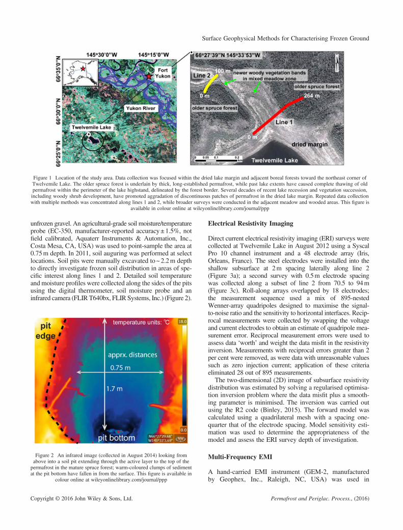
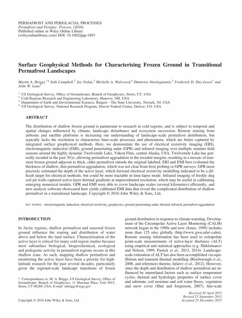
Figure 1 Location of the study area. Data collection was focused within the dried lake margin and adjacent boreal forests toward the northeast corner ofTwelvemile Lake. The older spruce forest is underlain by thick, long-established permafrost, while past lake extents have caused complete thawing of oldpermafrost within the perimeter of the lake highstand, delineated by the forest border. Several decades of recent lake recession and vegetation succession,including woody shrub development, have promoted aggradation of discontinuous patches of permafrost in the dried lake margin. Repeated data collectionwith multiple methods was concentrated along lines 1 and 2, while broader surveys were conducted in the adjacent meadow and wooded areas. This figure is

available in colour online at wileyonlinelibrary.com/journal/ppp

Surface Geophysical Methods for Characterising Frozen Ground

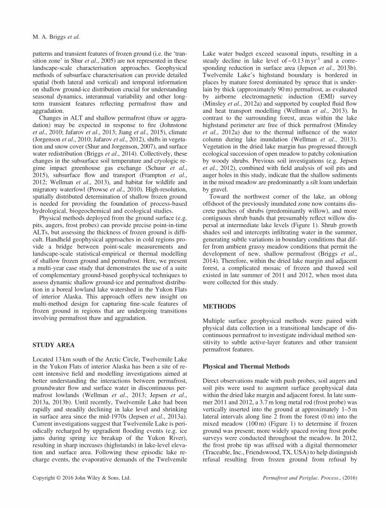
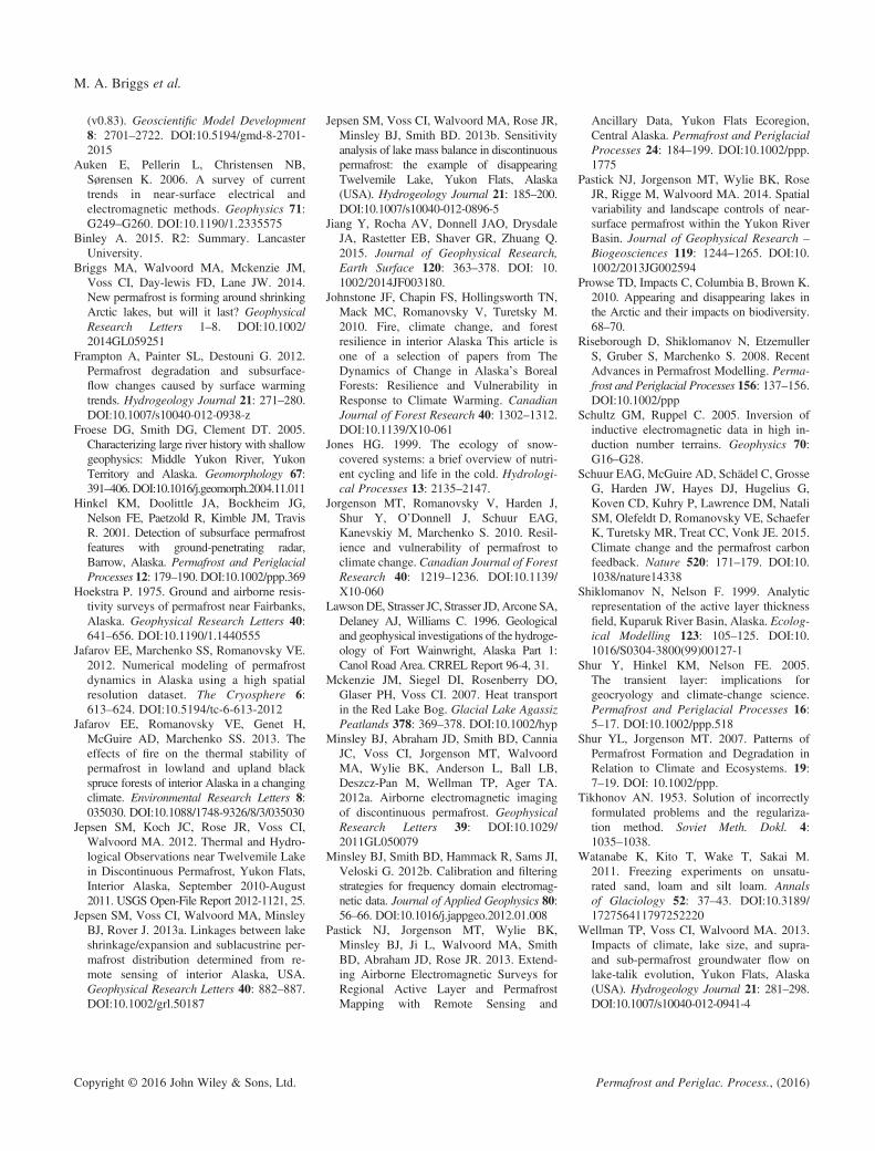
unfrozen gravel. An agricultural-grade soil moisture/temperatureprobe (EC-350, manufacturer-reported accuracy±1.5%, notfield calibrated, Aquaterr Instruments & Automation, Inc.,Costa Mesa, CA, USA) was used to point-sample the area at0.75m depth. In 2011, soil auguring was performed at selectlocations. Soil pits were manually excavated to~2.2m depthto directly investigate frozen soil distribution in areas of spe-cific interest along lines 1 and 2. Detailed soil temperatureand moisture profiles were collected along the sides of the pitsusing the digital thermometer, soil moisture probe and aninfrared camera (FLIR T640bx, FLIR Systems, Inc.) (Figure 2).

Figure 2 An infrared image (collected in August 2014) looking fromabove into a soil pit extending through the active layer to the top of thepermafrost in the mature spruce forest; warm-coloured clumps of sedimentat the pit bottom have fallen in from the surface. This figure is available in

colour online at wileyonlinelibrary.com/journal/ppp


Electrical Resistivity Imaging

Direct current electrical resistivity imaging (ERI) surveys werecollected at Twelvemile Lake in August 2012 using a SyscalPro 10 channel instrument and a 48 electrode array (Iris,Orleans, France). The steel electrodes were installed into theshallow subsurface at 2m spacing laterally along line 2(Figure 3a); a second survey with 0.5m electrode spacingwas collected along a subset of line 2 from 70.5 to 94m(Figure 3c). Roll-along arrays overlapped by 18 electrodes;the measurement sequence used a mix of 895-nestedWenner-array quadripoles designed to maximise the signal-to-noise ratio and the sensitivity to horizontal interfaces. Recip-rocal measurements were collected by swapping the voltageand current electrodes to obtain an estimate of quadripole mea-surement error. Reciprocal measurement errors were used toassess data ‘worth’ and weight the data misfit in the resistivityinversion. Measurements with reciprocal errors greater than 2per cent were removed, as were data with unreasonable valuessuch as zero injection current; application of these criteriaeliminated 28 out of 895 measurements.

The two-dimensional (2D) image of subsurface resistivitydistribution was estimated by solving a regularised optimisa-tion inversion problem where the data misfit plus a smooth-ing parameter is minimised. The inversion was carried outusing the R2 code (Binley, 2015). The forward model wascalculated using a quadrilateral mesh with a spacing one-quarter that of the electrode spacing. Model sensitivity esti-mation was used to determine the appropriateness of themodel and assess the ERI survey depth of investigation.

Multi-Frequency EMI

A hand-carried EMI instrument (GEM-2, manufacturedby Geophex, Inc., Raleigh, NC, USA) was used in


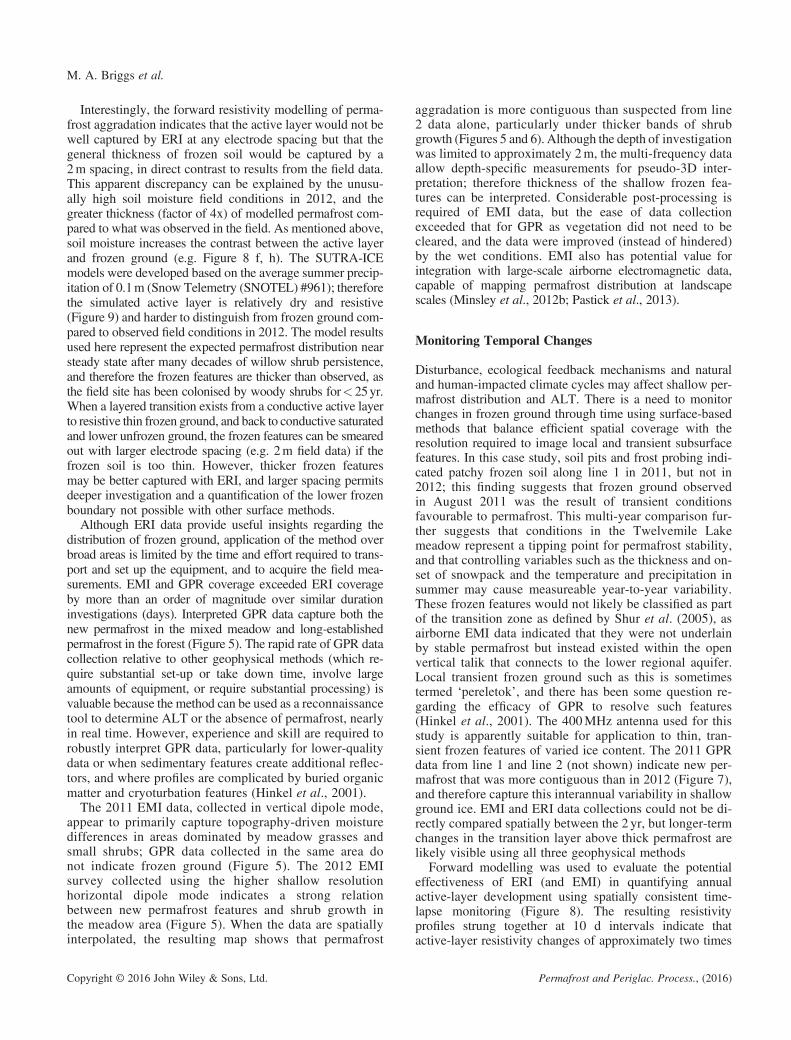
Figure 3 Line 2 data from combined methods: (a) inversion of 2012 electrical resistivity imaging (ERI) data with 2 m electrode spacing and related frost probedata; (b) 2011 GPR data from a subset of line 2 within the box indicated in (a); and (c) 2012 ERI data with 0.5 m electrode spacing from a subset of line 2within the box indicated in (a). The larger electrode spacing shows the zone of thick, old permafrost, deep gravel lens and predominantly thawed meadow areabut the new permafrost is not well captured. The closer electrode spacing along a subset of the line does capture the shallow, thin frozen features that correspond

with frost probe data. Although collected a year prior, the GPR data show a discontinuous reflector that corresponds with frost probe and 0.5m ERI data.

M. A. Briggs et al.

2011 and 2012 to measure the subsurface electrical con-ductivity of thawed and frozen ground in the northeastcorner area of Twelvemile Lake. Multi-frequency (n =7)quadrature data ranging from 1530 to 93 kHz were usedto estimate subsurface electrical conductivity from approx-imately 0 to 12m depth. The 2011 data were collected invertical dipole mode to maximise penetration depth overa range of soil conditions, while the 2012 data were pri-marily collected in horizontal dipole mode to maximisesensitivity to the shallow permafrost and active-layerfeatures.The calibration and inversion of frequency-domain EMI

data to accurately model subsurface conductivity can bechallenging. To address this, the US Geological Survey(USGS) Branch of Geophysics and Rutgers University aredeveloping codes for the inversion of frequency-domainelectromagnetic data. This new code is an extension of anEMI code previously described by Schultz and Ruppel(2005) with additional features and capabilities, includingone-dimensional (1D) laterally constrained electromagneticinversion, and regularisation and inversion in 2D or threedimensions (3D; user defined), although the forward modelsare in 1D, in order to minimise problems commonly associatedwith other unconstrained 1D approaches (e.g. Auken et al.,2006; Minsley et al., 2012b). A parallel inversion capabilitygreatly speeds the processing of large data-sets such as thatcollected at Twelvemile Lake. Prior to inversion, we filterand calibrate the data following the approach suggested byMinsley et al. (2012b). With this approach, the EMI dataare adjusted against a conductivity model derived fromERI surveys. Regularisation is implemented using theTikhonov (1953) approach.


GPR

GPR profiles were collected at Twelvemile Lake during the2011 and 2012 summer field campaigns. A GSSI SIR-3000control unit (Geophysical Survey Systems, Inc., Nashua,NH, USA) coupled with a GSSI model 5103 400MHzcentre-frequency bistatic antenna was used to assess: (1)the near-surface lithological properties; (2) the presence offrozen ground; and (3) the depth and spatial extent of the ac-tive layer. The antenna was hand towed at approximately0.5m s-1 across transects (e.g. lines 1 and 2) mostly clearedof surface vegetation to improve antenna coupling and sub-surface signal penetration. The antenna was oriented orthog-onal to the profile direction. The recording time windowranged from 80–140ns with 1024–2048 16 bit samples re-corded per trace. Profiles were recorded using time–rangegain, band pass filtering and stacking to reduce noise andimprove reflector signal-to-noise ratios. Distance marks ev-ery 10m were used to distance-normalise (rubber-sheet)each radar profile. All described GPR profile time rangesare two-way travel times (TWTT) unless otherwise noted.

Following distance normalisation, post-stack variable ve-locity migration was performed to convert reflection time todepth using RADAN (GSSI proprietary software) throughreflection hyperbola matching to estimate the spatial distri-bution of relative permittivity (ε′) and associated electro-magnetic wave velocities. The location of each 10m markwas also recorded with a handheld Garmin GPSMap62stc(Canton of Schaffhausen, Switzerland) and surface eleva-tion corrections were applied to each radar profile using pre-viously collected high vertical resolution airborne lightdetection and ranging (lidar) data.



GPR waveform polarity (phase) interpretations of reflec-tion triplet sequences were performed as suggested byArcone et al. (1995). That is, for the model antenna used,the polarity of the first three half-cycle responses of areflecting horizon or target indicates the contrast in the ε′between layers. The differences in ε′ of liquid water (~80),permafrost (~5.3), ice (~3.2), air (1) and sediments (~5–26depending on moisture content) provide sufficient contrastto interpret triplet sequences in terms of differences indielectric properties at reflector boundaries. A positive (+ - +)triplet suggests that the deeper layer or target has a higher ε′than the overlying layer (i.e. more water or unfrozen), and anegative (-+ -) triplet suggests that the deeper layer or targethas a lower ε′ (i.e. less water or frozen).

Forward Modelling of Electrical Resistivity

To demonstrate the utility of the direct current ERI methodto describe fine-scale permafrost features, synthetic resistivitymodels were developed based on typical silt loam soil condi-tions expected within the Twelvemile Lake dried margin(Jepsen et al., 2012). Seasonal frozen ground and permafrostdynamics were evaluated using the USGS SUTRA-ICEmodel that simulates coupled fluid flow and energy transportfor variably saturated conditions with freeze/thaw (Mckenzieet al., 2007). The 1D SUTRA-ICE numerical simulationswere designed to investigate the subsurface cryologic re-sponse to lake recession and vegetation succession in a coldregion landscape (see Briggs et al., 2014, for a full descriptionof the numerical analysis). SUTRA-ICE model output, in-cluding information on ice and liquid water saturation andtemperature, was then converted to geoelectrical resistivityfields based on a version of Archie’s (1942) law, a widelyused petrophysical relation modified to enable considerationof liquid and solid water phases. This relationship assumesthat soil bulk resistivity ρ (Ωm) is controlled by ionic conduc-tion of the pore fluid in a two-phase medium:

ρ ¼ αρwθ-mSw

-n (1)

For this work (and SUTRA-ICE modelling), a soil porosity(θ) of 0.46 for silt loam soils was assumed, based on labora-tory measurements of similar soils (Watanabe et al., 2011).The fraction of pore space filled with liquid water (Sw) wasobtained from the SUTRA-ICE model output; the ice is as-sumed to have no electrical conduction capability, similar toair-filled pore space. The empirically determined Archie’slaw parameters α, m and n were initially estimated as 1, 1.5and 1.8, respectively (based on typical published values),and manually optimised to match a subset of collocated bulkresistivity, fluid conductivity and saturation field data ac-quired in 2012 at a depth of 0.75m along line 1. The resistiv-ity of the water ρw, 23.3Ωm is from a 2012 field measurementof a water sample obtained from a test pit along line 1 using anOakton handheld water conductivity meter (Oakton Instru-ments, Vernon Hills, IL, USA).


Soil resistivity was adjusted for temperature using the re-lationship:

ρ ¼ ρo1þ αt T � Toð Þ (2)

where αt is the temperature coefficient 0.025K-1 and T-To isthe change in temperature. In this study, other temperature-dependent effects on the resistivity of soil (including tem-perature effects below the freezing point and ion exclusion)were not considered, because the conditions modelled bySUTRA-ICE were typically close to the freezing point andice saturation did not exceed 0.6 due to the relatively largepercentage of liquid water (16.6%) expected in silt loamsat temperatures as low as -20 °C (Watanabe et al., 2011).Resistivity was determined using Equations 1 and 2 for nu-merical model output for the lake recession scenario withwillow shrub influence that promotes permafrost aggrada-tion (‘willow’ model) and open meadow conditions withinthe dried lake boundary before ecological succession(‘ambient’ model); model output is at 10 d incrementsover 1 yr.

Quantitative evaluation of ERI resolution and depth of in-vestigation based on modelling exercises for hypothetical,yet realistic field scenarios can guide planning of ERI sur-veys and support interpretation of ERI results. Here, weevaluate ERI resolution and depth of investigation as a func-tion of electrode spacing, for scenarios based on theSUTRA-ICE model output and Equations 1 and 2. We usethe R2 code forward resistivity model to simulate hypotheticalERI data for snapshots in late August (corresponding withfieldwork timing) for 0.5, 1.0, 2 and 4m electrode spacingsurveys. The willow model has several metres of new, shallowpermafrost in late summer, whereas the ambient model hasonly a maximum ice saturation of about 5 per cent at the capil-lary fringe of the 3m deep water table during the same timeframe. The willow condition was applied to the left half ofthe domain and the ambient condition was applied to the righthalf, representing mixed meadow conditions of discretewoody vegetation clumps and shrub bands (willow condi-tion) within the grassy area (ambient condition). The totaldomain width/depth varied based on electrode spacingand a constant number of virtual electrodes (n = 48); there-fore for larger electrode spacing, the synthetic domain wasboth wider and deeper. To replicate typical field dataerrors, 2 per cent random noise was applied to the syntheticmeasurements and a resistivity field was estimated for eachof the four variable spacing models using the same inver-sion method as the field case.

RESULTS

Data pertaining to shallow frozen ground distribution fromphysical, thermal, radar and electrical methods are presentedbelow. ERI forward resistivity modelling based on SUTRA-ICE model output is used to guide field data interpretation


M. A. Briggs et al.

and survey designs for future applications by examining thegeophysical response to ‘known’ conditions.

Physical Methods

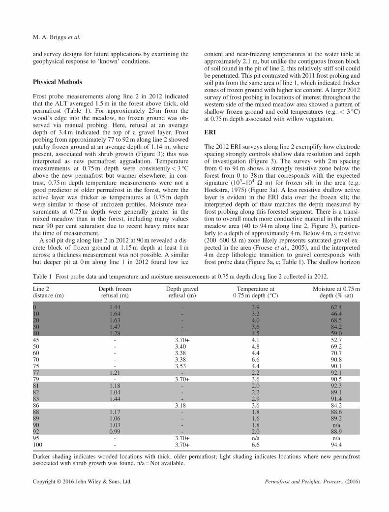
Frost probe measurements along line 2 in 2012 indicatedthat the ALT averaged 1.5m in the forest above thick, oldpermafrost (Table 1). For approximately 25m from thewood’s edge into the meadow, no frozen ground was ob-served via manual probing. Here, refusal at an averagedepth of 3.4m indicated the top of a gravel layer. Frostprobing from approximately 77 to 92m along line 2 showedpatchy frozen ground at an average depth of 1.14 m, wherepresent, associated with shrub growth (Figure 3); this wasinterpreted as new permafrost aggradation. Temperaturemeasurements at 0.75m depth were consistently<3 °Cabove the new permafrost but warmer elsewhere; in con-trast, 0.75m depth temperature measurements were not agood predictor of older permafrost in the forest, where theactive layer was thicker as temperatures at 0.75m depthwere similar to those of unfrozen profiles. Moisture mea-surements at 0.75m depth were generally greater in themixed meadow than in the forest, including many valuesnear 90 per cent saturation due to recent heavy rains nearthe time of measurement.A soil pit dug along line 2 in 2012 at 90m revealed a dis-

crete block of frozen ground at 1.15m depth at least 1macross; a thickness measurement was not possible. A similarbut deeper pit at 0m along line 1 in 2012 found low ice

Table 1 Frost probe data and temperature and moisture measureme

Line 2distance (m)

Depth frozenrefusal (m)

Depth gravelrefusal (m)

0 1.44 -10 1.64 -20 1.63 -30 1.47 -40 1.28 -45 - 3.70+50 - 3.4060 - 3.3870 - 3.3875 - 3.5377 1.21 -79 - 3.70+81 1.18 -82 1.04 -83 1.44 -86 - 3.1888 1.17 -89 1.06 -90 1.03 -92 0.99 -95 - 3.70+100 - 3.70+

Darker shading indicates wooded locations with thick, older permaassociated with shrub growth was found. n/a =Not available.


content and near-freezing temperatures at the water table atapproximately 2.1 m, but unlike the contiguous frozen blockof soil found in the pit of line 2, this relatively stiff soil couldbe penetrated. This pit contrasted with 2011 frost probing andsoil pits from the same area of line 1, which indicated thickerzones of frozen ground with higher ice content. A larger 2012survey of frost probing in locations of interest throughout thewestern side of the mixed meadow area showed a pattern ofshallow frozen ground and cold temperatures (e.g. < 3 °C)at 0.75m depth associated with willow vegetation.

ERI

The 2012 ERI surveys along line 2 exemplify how electrodespacing strongly controls shallow data resolution and depthof investigation (Figure 3). The survey with 2m spacingfrom 0 to 94m shows a strongly resistive zone below theforest from 0 to 38m that corresponds with the expectedsignature (103–104 Ω m) for frozen silt in the area (e.g.Hoekstra, 1975) (Figure 3a). A less resistive shallow activelayer is evident in the ERI data over the frozen silt; theinterpreted depth of thaw matches the depth measured byfrost probing along this forested segment. There is a transi-tion to overall much more conductive material in the mixedmeadow area (40 to 94m along line 2, Figure 3), particu-larly to a depth of approximately 4m. Below 4m, a resistive(200–600 Ω m) zone likely represents saturated gravel ex-pected in the area (Froese et al., 2005), and the interpreted4m deep lithologic transition to gravel corresponds withfrost probe data (Figure 3a, c; Table 1). The shallow horizon

nts at 0.75m depth along line 2 collected in 2012.

Temperature at0.75m depth (°C)

Moisture at 0.75mdepth (% sat)

3.9 62.43.2 46.44.0 68.53.6 84.24.5 59.04.1 52.74.8 69.24.4 70.76.6 90.84.4 90.12.2 92.13.6 90.52.0 92.32.2 89.12.9 91.43.6 84.21.8 88.61.6 89.21.8 n/a2.0 88.9n/a n/a6.6 94.4

frost; light shading indicates locations where new permafrost



(<4m depth) in the meadow is an order of magnitude lessresistive, reflecting predominantly unfrozen silt loam withhigh moisture content (Table 1). Local permafrost aggrada-tion identified with frost probing is not captured well by the2m electrode spacing, although there are some indicationsof subtle variation in resistivity in the new permafrost area(Figure 3a inset box).The ERI survey using 0.5m electrode spacing from 70 to

94m shows shallow resistive lenses (200–400 Ω m) thatcorrespond with frost probe data, indicating permafrost ag-gradation since the retreat of the lake (Figure 3b). Lateralbreaks in the resistive lenses also correspond to places werethawed ground was identified via probing. The ERI data in-dicate that the newly aggraded permafrost is approximately1m thick and exists wholly within the upper 2m. AlthoughERI data resolution has seemingly been greatly improvedwith the closer electrode spacing, the depth of investigationis limited to approximately 3m. Data from both electrodespacings were used to calibrate EMI data to the study areafield conditions.

Multi-Frequency EMI

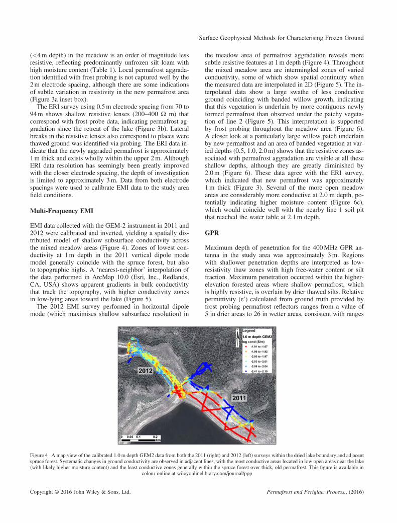
EMI data collected with the GEM-2 instrument in 2011 and2012 were calibrated and inverted, yielding a spatially dis-tributed model of shallow subsurface conductivity acrossthe mixed meadow areas (Figure 4). Zones of lowest con-ductivity at 1m depth in the 2011 vertical dipole modemodel generally coincide with the spruce forest, but alsoto topographic highs. A ‘nearest-neighbor’ interpolation ofthe data performed in ArcMap 10.0 (Esri, Inc., Redlands,CA, USA) shows apparent gradients in bulk conductivitythat track the topography, with higher conductivity zonesin low-lying areas toward the lake (Figure 5).The 2012 EMI survey performed in horizontal dipole

mode (which maximises shallow subsurface resolution) in

Figure 4 A map view of the calibrated 1.0 m depth GEM2 data from both the 201spruce forest. Systematic changes in ground conductivity are observed in adjacent(with likely higher moisture content) and the least conductive zones generally wi

colour online at wileyonlinel


the meadow area of permafrost aggradation reveals moresubtle resistive features at 1m depth (Figure 4). Throughoutthe mixed meadow area are intermingled zones of variedconductivity, some of which show spatial continuity whenthe measured data are interpolated in 2D (Figure 5). The in-terpolated data show a large swathe of less conductiveground coinciding with banded willow growth, indicatingthat this vegetation is underlain by more contiguous newlyformed permafrost than observed under the patchy vegeta-tion of line 2 (Figure 5). This interpretation is supportedby frost probing throughout the meadow area (Figure 6).A closer look at a particularly large willow patch underlainby new permafrost and an area of banded vegetation at var-ied depths (0.5, 1.0, 2.0m) shows that the resistive zones as-sociated with permafrost aggradation are visible at all theseshallow depths, although they are greatly diminished by2.0m (Figure 6). These data agree with the ERI survey,which indicated that new permafrost was approximately1m thick (Figure 3). Several of the more open meadowareas are considerably more conductive at 2.0 m depth, po-tentially indicating higher moisture content (Figure 6c),which would coincide well with the nearby line 1 soil pitthat reached the water table at 2.1m depth.

GPR

Maximum depth of penetration for the 400MHz GPR an-tenna in the study area was approximately 3m. Regionswith shallower penetration depths are interpreted as low-resistivity thaw zones with high free-water content or siltfraction. Maximum penetration occurred within the higher-elevation forested areas where shallow permafrost, whichis highly resistive, is overlain by drier thawed silts. Relativepermittivity (ε′) calculated from ground truth provided byfrost probing permafrost reflectors ranges from a value of5 in drier areas to 26 in wetter areas, consistent with ranges

1 (right) and 2012 (left) surveys within the dried lake boundary and adjacentlines, with the most conductive areas located in low open areas near the lakethin the spruce forest over thick, old permafrost. This figure is available inibrary.com/journal/ppp


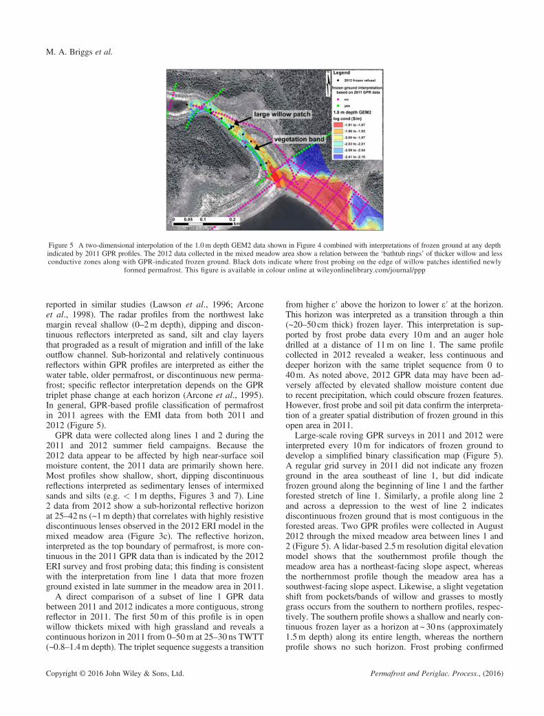
Figure 5 A two-dimensional interpolation of the 1.0 m depth GEM2 data shown in Figure 4 combined with interpretations of frozen ground at any depthindicated by 2011 GPR profiles. The 2012 data collected in the mixed meadow area show a relation between the ‘bathtub rings’ of thicker willow and lessconductive zones along with GPR-indicated frozen ground. Black dots indicate where frost probing on the edge of willow patches identified newly

formed permafrost. This figure is available in colour online at wileyonlinelibrary.com/journal/ppp

M. A. Briggs et al.

reported in similar studies (Lawson et al., 1996; Arconeet al., 1998). The radar profiles from the northwest lakemargin reveal shallow (0–2m depth), dipping and discon-tinuous reflectors interpreted as sand, silt and clay layersthat prograded as a result of migration and infill of the lakeoutflow channel. Sub-horizontal and relatively continuousreflectors within GPR profiles are interpreted as either thewater table, older permafrost, or discontinuous new perma-frost; specific reflector interpretation depends on the GPRtriplet phase change at each horizon (Arcone et al., 1995).In general, GPR-based profile classification of permafrostin 2011 agrees with the EMI data from both 2011 and2012 (Figure 5).GPR data were collected along lines 1 and 2 during the

2011 and 2012 summer field campaigns. Because the2012 data appear to be affected by high near-surface soilmoisture content, the 2011 data are primarily shown here.Most profiles show shallow, short, dipping discontinuousreflections interpreted as sedimentary lenses of intermixedsands and silts (e.g. < 1m depths, Figures 3 and 7). Line2 data from 2012 show a sub-horizontal reflective horizonat 25–42 ns (~1m depth) that correlates with highly resistivediscontinuous lenses observed in the 2012 ERI model in themixed meadow area (Figure 3c). The reflective horizon,interpreted as the top boundary of permafrost, is more con-tinuous in the 2011 GPR data than is indicated by the 2012ERI survey and frost probing data; this finding is consistentwith the interpretation from line 1 data that more frozenground existed in late summer in the meadow area in 2011.A direct comparison of a subset of line 1 GPR data

between 2011 and 2012 indicates a more contiguous, strongreflector in 2011. The first 50m of this profile is in openwillow thickets mixed with high grassland and reveals acontinuous horizon in 2011 from 0–50m at 25–30 ns TWTT(~0.8–1.4m depth). The triplet sequence suggests a transition


from higher ε′ above the horizon to lower ε′ at the horizon.This horizon was interpreted as a transition through a thin(~20–50cm thick) frozen layer. This interpretation is sup-ported by frost probe data every 10m and an auger holedrilled at a distance of 11m on line 1. The same profilecollected in 2012 revealed a weaker, less continuous anddeeper horizon with the same triplet sequence from 0 to40m. As noted above, 2012 GPR data may have been ad-versely affected by elevated shallow moisture content dueto recent precipitation, which could obscure frozen features.However, frost probe and soil pit data confirm the interpreta-tion of a greater spatial distribution of frozen ground in thisopen area in 2011.

Large-scale roving GPR surveys in 2011 and 2012 wereinterpreted every 10m for indicators of frozen ground todevelop a simplified binary classification map (Figure 5).A regular grid survey in 2011 did not indicate any frozenground in the area southeast of line 1, but did indicatefrozen ground along the beginning of line 1 and the fartherforested stretch of line 1. Similarly, a profile along line 2and across a depression to the west of line 2 indicatesdiscontinuous frozen ground that is most contiguous in theforested areas. Two GPR profiles were collected in August2012 through the mixed meadow area between lines 1 and2 (Figure 5). A lidar-based 2.5m resolution digital elevationmodel shows that the southernmost profile though themeadow area has a northeast-facing slope aspect, whereasthe northernmost profile though the meadow area has asouthwest-facing slope aspect. Likewise, a slight vegetationshift from pockets/bands of willow and grasses to mostlygrass occurs from the southern to northern profiles, respec-tively. The southern profile shows a shallow and nearly con-tinuous frozen layer as a horizon at ~ 30 ns (approximately1.5m depth) along its entire length, whereas the northernprofile shows no such horizon. Frost probing confirmed


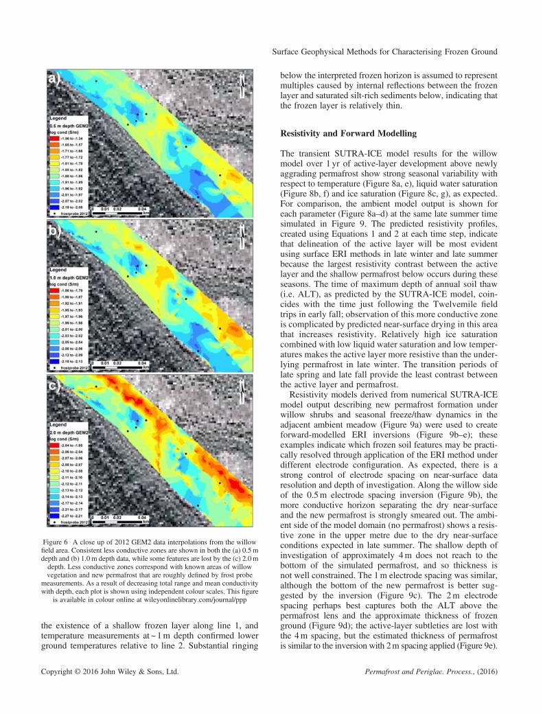
Figure 6 A close up of 2012 GEM2 data interpolations from the willowfield area. Consistent less conductive zones are shown in both the (a) 0.5 mdepth and (b) 1.0 m depth data, while some features are lost by the (c) 2.0 mdepth. Less conductive zones correspond with known areas of willowvegetation and new permafrost that are roughly defined by frost probe

measurements. As a result of decreasing total range and mean conductivitywith depth, each plot is shown using independent colour scales. This figure

is available in colour online at wileyonlinelibrary.com/journal/ppp


the existence of a shallow frozen layer along line 1, andtemperature measurements at ~ 1m depth confirmed lowerground temperatures relative to line 2. Substantial ringing


below the interpreted frozen horizon is assumed to representmultiples caused by internal reflections between the frozenlayer and saturated silt-rich sediments below, indicating thatthe frozen layer is relatively thin.

Resistivity and Forward Modelling

The transient SUTRA-ICE model results for the willowmodel over 1 yr of active-layer development above newlyaggrading permafrost show strong seasonal variability withrespect to temperature (Figure 8a, e), liquid water saturation(Figure 8b, f) and ice saturation (Figure 8c, g), as expected.For comparison, the ambient model output is shown foreach parameter (Figure 8a–d) at the same late summer timesimulated in Figure 9. The predicted resistivity profiles,created using Equations 1 and 2 at each time step, indicatethat delineation of the active layer will be most evidentusing surface ERI methods in late winter and late summerbecause the largest resistivity contrast between the activelayer and the shallow permafrost below occurs during theseseasons. The time of maximum depth of annual soil thaw(i.e. ALT), as predicted by the SUTRA-ICE model, coin-cides with the time just following the Twelvemile fieldtrips in early fall; observation of this more conductive zoneis complicated by predicted near-surface drying in this areathat increases resistivity. Relatively high ice saturationcombined with low liquid water saturation and low temper-atures makes the active layer more resistive than the under-lying permafrost in late winter. The transition periods oflate spring and late fall provide the least contrast betweenthe active layer and permafrost.

Resistivity models derived from numerical SUTRA-ICEmodel output describing new permafrost formation underwillow shrubs and seasonal freeze/thaw dynamics in theadjacent ambient meadow (Figure 9a) were used to createforward-modelled ERI inversions (Figure 9b–e); theseexamples indicate which frozen soil features may be practi-cally resolved through application of the ERI method underdifferent electrode configuration. As expected, there is astrong control of electrode spacing on near-surface dataresolution and depth of investigation. Along the willow sideof the 0.5m electrode spacing inversion (Figure 9b), themore conductive horizon separating the dry near-surfaceand the new permafrost is strongly smeared out. The ambi-ent side of the model domain (no permafrost) shows a resis-tive zone in the upper metre due to the dry near-surfaceconditions expected in late summer. The shallow depth ofinvestigation of approximately 4m does not reach to thebottom of the simulated permafrost, and so thickness isnot well constrained. The 1m electrode spacing was similar,although the bottom of the new permafrost is better sug-gested by the inversion (Figure 9c). The 2m electrodespacing perhaps best captures both the ALT above thepermafrost lens and the approximate thickness of frozenground (Figure 9d); the active-layer subtleties are lost withthe 4m spacing, but the estimated thickness of permafrostis similar to the inversion with 2m spacing applied (Figure 9e).


Figure 7 GPR profiles from 0 to 50 m along line 1 in 2011 and 2012. The stronger reflective horizon observed in 2011 indicates a more contiguous and higherice-content frozen layer at approximately 1 m depth compared to that in 2012; this interpretation was supported by physical measurements. TWTT= Two-way

travel time.

M. A. Briggs et al.

The low ice content (approximately 5%) zone that develops inthe ambient meadow models near the capillary fringe is notresolved in any inversion.

DISCUSSION

The complex permafrost distribution around TwelvemileLake allowed the direct comparison, augmented by forwardresistivity modelling, of several geophysical techniques inevaluating shallow frozen ground dynamics. ERI methodsprovided the most robust 2D images of permafrost alongdesignated transects, but EMI and GPR methods enabledefficient coverage of large areas and also revealed important

Figure 8 Distributions by depth for simulated late summer in Figure 7 are shownliquid saturation; and (c) ice saturation; these parameters drive subsurface resistivifor the willow model in panels (e)–(g) at 10 d intervals, and are used to calcula

corresponds to the timing of model output shown in (a)–(d). This figure


active-layer and permafrost features. The existence of tran-sient frozen ground was evident by comparison betweenthe 2011 and 2012 surveys in EMI and GPR data, interpreta-tions that are supported by physical measurements, indicatingthe ability of these methods to delineate thin, transient anddiscontinuous frozen ground features.

Evaluating Shallow Frozen Features

The upper boundary of the thick (up to approximately 90m)permafrost expected below the mature forests outside of thehistorical lake highstand boundary (Minsley et al., 2012a) isobserved with all three geophysical methods in both 2011and 2012. The 2012 ERI data (2m electrode spacing)

for the willow and ambient models for the parameters: (a) temperature; (b)ty shown in panel (d). Temporal distributions of these parameters are shownte the expected resistivity profile time series shown in (h). The open boxis available in colour online at wileyonlinelibrary.com/journal/ppp


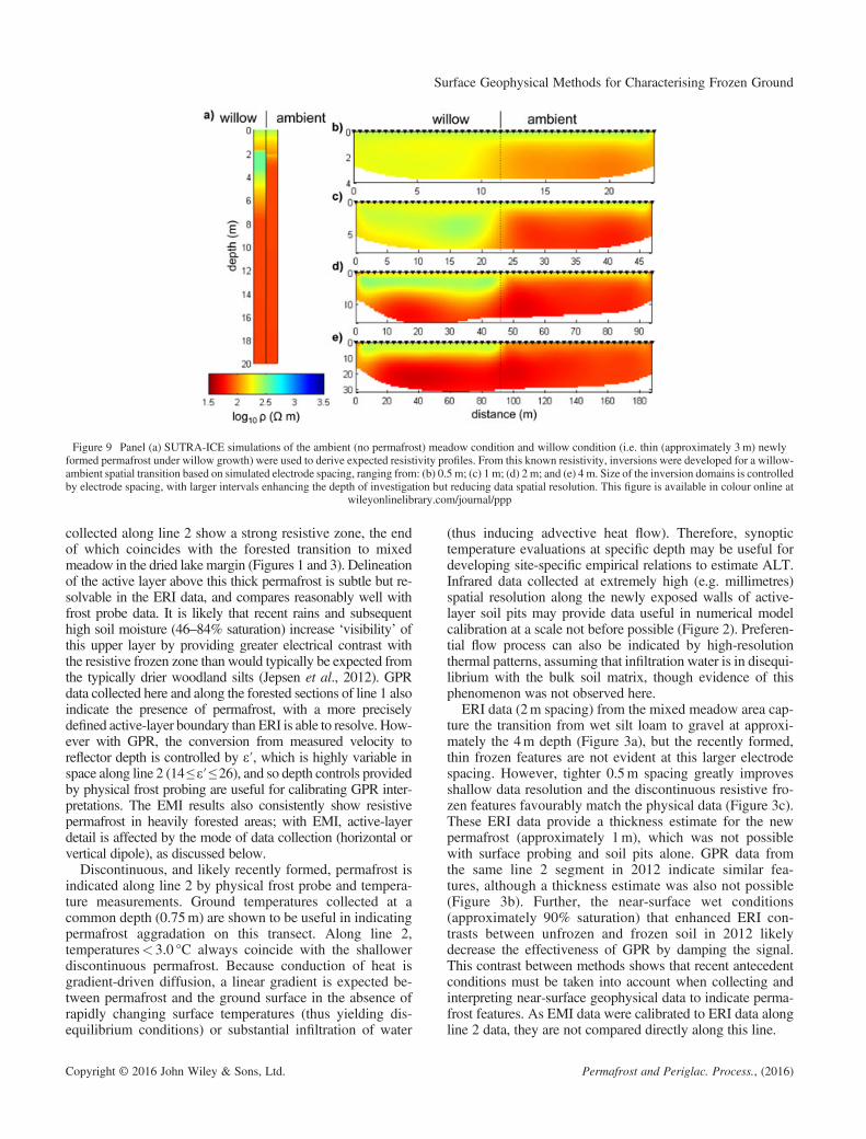
Figure 9 Panel (a) SUTRA-ICE simulations of the ambient (no permafrost) meadow condition and willow condition (i.e. thin (approximately 3 m) newlyformed permafrost under willow growth) were used to derive expected resistivity profiles. From this known resistivity, inversions were developed for a willow-ambient spatial transition based on simulated electrode spacing, ranging from: (b) 0.5 m; (c) 1 m; (d) 2 m; and (e) 4 m. Size of the inversion domains is controlledby electrode spacing, with larger intervals enhancing the depth of investigation but reducing data spatial resolution. This figure is available in colour online at

wileyonlinelibrary.com/journal/ppp


collected along line 2 show a strong resistive zone, the endof which coincides with the forested transition to mixedmeadow in the dried lakemargin (Figures 1 and 3). Delineationof the active layer above this thick permafrost is subtle but re-solvable in the ERI data, and compares reasonably well withfrost probe data. It is likely that recent rains and subsequenthigh soil moisture (46–84% saturation) increase ‘visibility’ ofthis upper layer by providing greater electrical contrast withthe resistive frozen zone than would typically be expected fromthe typically drier woodland silts (Jepsen et al., 2012). GPRdata collected here and along the forested sections of line 1 alsoindicate the presence of permafrost, with a more preciselydefined active-layer boundary than ERI is able to resolve. How-ever with GPR, the conversion from measured velocity toreflector depth is controlled by ε′, which is highly variable inspace along line 2 (14≤ ε′≤ 26), and so depth controls providedby physical frost probing are useful for calibrating GPR inter-pretations. The EMI results also consistently show resistivepermafrost in heavily forested areas; with EMI, active-layerdetail is affected by the mode of data collection (horizontal orvertical dipole), as discussed below.Discontinuous, and likely recently formed, permafrost is

indicated along line 2 by physical frost probe and tempera-ture measurements. Ground temperatures collected at acommon depth (0.75m) are shown to be useful in indicatingpermafrost aggradation on this transect. Along line 2,temperatures<3.0 °C always coincide with the shallowerdiscontinuous permafrost. Because conduction of heat isgradient-driven diffusion, a linear gradient is expected be-tween permafrost and the ground surface in the absence ofrapidly changing surface temperatures (thus yielding dis-equilibrium conditions) or substantial infiltration of water


(thus inducing advective heat flow). Therefore, synoptictemperature evaluations at specific depth may be useful fordeveloping site-specific empirical relations to estimate ALT.Infrared data collected at extremely high (e.g. millimetres)spatial resolution along the newly exposed walls of active-layer soil pits may provide data useful in numerical modelcalibration at a scale not before possible (Figure 2). Preferen-tial flow process can also be indicated by high-resolutionthermal patterns, assuming that infiltration water is in disequi-librium with the bulk soil matrix, though evidence of thisphenomenon was not observed here.

ERI data (2m spacing) from the mixed meadow area cap-ture the transition from wet silt loam to gravel at approxi-mately the 4m depth (Figure 3a), but the recently formed,thin frozen features are not evident at this larger electrodespacing. However, tighter 0.5m spacing greatly improvesshallow data resolution and the discontinuous resistive fro-zen features favourably match the physical data (Figure 3c).These ERI data provide a thickness estimate for the newpermafrost (approximately 1m), which was not possiblewith surface probing and soil pits alone. GPR data fromthe same line 2 segment in 2012 indicate similar fea-tures, although a thickness estimate was also not possible(Figure 3b). Further, the near-surface wet conditions(approximately 90% saturation) that enhanced ERI con-trasts between unfrozen and frozen soil in 2012 likelydecrease the effectiveness of GPR by damping the signal.This contrast between methods shows that recent antecedentconditions must be taken into account when collecting andinterpreting near-surface geophysical data to indicate perma-frost features. As EMI data were calibrated to ERI data alongline 2 data, they are not compared directly along this line.


M. A. Briggs et al.

Interestingly, the forward resistivity modelling of perma-frost aggradation indicates that the active layer would not bewell captured by ERI at any electrode spacing but that thegeneral thickness of frozen soil would be captured by a2m spacing, in direct contrast to results from the field data.This apparent discrepancy can be explained by the unusu-ally high soil moisture field conditions in 2012, and thegreater thickness (factor of 4x) of modelled permafrost com-pared to what was observed in the field. As mentioned above,soil moisture increases the contrast between the active layerand frozen ground (e.g. Figure 8 f, h). The SUTRA-ICEmodels were developed based on the average summer precip-itation of 0.1m (Snow Telemetry (SNOTEL) #961); thereforethe simulated active layer is relatively dry and resistive(Figure 9) and harder to distinguish from frozen ground com-pared to observed field conditions in 2012. The model resultsused here represent the expected permafrost distribution nearsteady state after many decades of willow shrub persistence,and therefore the frozen features are thicker than observed, asthe field site has been colonised by woody shrubs for<25yr.When a layered transition exists from a conductive active layerto resistive thin frozen ground, and back to conductive saturatedand lower unfrozen ground, the frozen features can be smearedout with larger electrode spacing (e.g. 2m field data) if thefrozen soil is too thin. However, thicker frozen featuresmay be better captured with ERI, and larger spacing permitsdeeper investigation and a quantification of the lower frozenboundary not possible with other surface methods.Although ERI data provide useful insights regarding the

distribution of frozen ground, application of the method overbroad areas is limited by the time and effort required to trans-port and set up the equipment, and to acquire the field mea-surements. EMI and GPR coverage exceeded ERI coverageby more than an order of magnitude over similar durationinvestigations (days). Interpreted GPR data capture both thenew permafrost in the mixed meadow and long-establishedpermafrost in the forest (Figure 5). The rapid rate of GPR datacollection relative to other geophysical methods (which re-quire substantial set-up or take down time, involve largeamounts of equipment, or require substantial processing) isvaluable because the method can be used as a reconnaissancetool to determine ALT or the absence of permafrost, nearlyin real time. However, experience and skill are required torobustly interpret GPR data, particularly for lower-qualitydata or when sedimentary features create additional reflec-tors, and where profiles are complicated by buried organicmatter and cryoturbation features (Hinkel et al., 2001).The 2011 EMI data, collected in vertical dipole mode,

appear to primarily capture topography-driven moisturedifferences in areas dominated by meadow grasses andsmall shrubs; GPR data collected in the same area donot indicate frozen ground (Figure 5). The 2012 EMIsurvey collected using the higher shallow resolutionhorizontal dipole mode indicates a strong relationbetween new permafrost features and shrub growth inthe meadow area (Figure 5). When the data are spatiallyinterpolated, the resulting map shows that permafrost


aggradation is more contiguous than suspected from line2 data alone, particularly under thicker bands of shrubgrowth (Figures 5 and 6). Although the depth of investigationwas limited to approximately 2m, the multi-frequency dataallow depth-specific measurements for pseudo-3D inter-pretation; therefore thickness of the shallow frozen fea-tures can be interpreted. Considerable post-processing isrequired of EMI data, but the ease of data collectionexceeded that for GPR as vegetation did not need to becleared, and the data were improved (instead of hindered)by the wet conditions. EMI also has potential value forintegration with large-scale airborne electromagnetic data,capable of mapping permafrost distribution at landscapescales (Minsley et al., 2012b; Pastick et al., 2013).

Monitoring Temporal Changes

Disturbance, ecological feedback mechanisms and naturaland human-impacted climate cycles may affect shallow per-mafrost distribution and ALT. There is a need to monitorchanges in frozen ground through time using surface-basedmethods that balance efficient spatial coverage with theresolution required to image local and transient subsurfacefeatures. In this case study, soil pits and frost probing indi-cated patchy frozen soil along line 1 in 2011, but not in2012; this finding suggests that frozen ground observedin August 2011 was the result of transient conditionsfavourable to permafrost. This multi-year comparison fur-ther suggests that conditions in the Twelvemile Lakemeadow represent a tipping point for permafrost stability,and that controlling variables such as the thickness and on-set of snowpack and the temperature and precipitation insummer may cause measureable year-to-year variability.These frozen features would not likely be classified as partof the transition zone as defined by Shur et al. (2005), asairborne EMI data indicated that they were not underlainby stable permafrost but instead existed within the openvertical talik that connects to the lower regional aquifer.Local transient frozen ground such as this is sometimestermed ‘pereletok’, and there has been some question re-garding the efficacy of GPR to resolve such features(Hinkel et al., 2001). The 400MHz antenna used for thisstudy is apparently suitable for application to thin, tran-sient frozen features of varied ice content. The 2011 GPRdata from line 1 and line 2 (not shown) indicate new per-mafrost that was more contiguous than in 2012 (Figure 7),and therefore capture this interannual variability in shallowground ice. EMI and ERI data collections could not be di-rectly compared spatially between the 2 yr, but longer-termchanges in the transition layer above thick permafrost arelikely visible using all three geophysical methods

Forward modelling was used to evaluate the potentialeffectiveness of ERI (and EMI) in quantifying annualactive-layer development using spatially consistent time-lapse monitoring (Figure 8). The resulting resistivityprofiles strung together at 10 d intervals indicate thatactive-layer resistivity changes of approximately two times



can be expected when the effects of ion exclusion duringfreezing are neglected. The strongest contrasts between theactive layer and permafrost occur in late summer(Figure 8h); hence the applicability of ERI for active-layerdynamics may be seasonally limited.To fully understand the capabilities of ERI, it is not suffi-

cient to solely consider resistivity contrast; rather, array de-sign, survey layout and data measurement errors playimportant roles that contribute to overall model resolutionand depth of investigation. Figure 9 shows inversion resultsfor a site with a spatial transition between open grassy areas(ambient model) and woody shrub (willow model) condi-tions, representative of the observed mixed meadow. Inver-sion results indicate that the active layer is not well resolvedwhen the active layer is relatively dry (Figure 9), regardlessof the electrode spacing considered. This result indicatesthat during transitional times of the year shallow, thin fea-tures may be even more difficult to resolve, but that en-hanced ground saturation after precipitation events can aidcontrast between frozen and unfrozen soil. Interestingly,when the active layer freezes to maximum depth in mid-latewinter, this layer is approximately 40 per cent more resistivethan the permafrost below due to the additive effects of lowtemperature and low moisture content. With time-lapse ERI,analysis of difference maps often indicates processes notobvious in ‘snapshot’ data alone, and may be more usefulin identifying changes in frozen ground features throughoutthe year and after disturbance.

CONCLUSIONS

The complicated distribution of frozen ground and perma-frost around Twelvemile Lake in the Yukon Flats of interiorAlaska provides an opportunity to integrate several surfacegeophysical methods (ERI, EMI, GPR, infrared) to evaluateALT and longer-term transient frozen ground features, andhighlight the methods’ strengths and shortcomings. Datacollected over several years indicated that thick, stable per-mafrost exists below mature forest adjacent to an area ofmixed meadow within the dried lake boundary with newlyaggraded permafrost and seasonally frozen ground. Theactive layer was thinner over the newly formed permafrostfeatures, conditions that were confirmed with direct mea-surement of thaw depth and temperature.Transferable lessons from this case study include:

1. ERI provided the best-constrained thickness estimates ofthin, shallow permafrost features, followed by EMI.


2. Field data and forward resistivity modelling indicate thatprecise ALT estimates may not be possible withsnapshot-in-time ERI and EMI surveys, though contrastis enhanced after rain events; GPR more clearly showedthe upper interface of frozen ground, but the conversionto true depth is sensitive to the relative permittivity (ε′)parameter, which may be highly spatially variable.

3. Practical spatial coverage was highest with EMI,followed by GPR; therefore, these two methods are mostapplicable to landscape-scale evaluations of transientfrozen features relevant to research regarding shallowgroundwater flow and surface water exchange.

4. GPR data can be evaluated in near-real time by an expe-rienced practitioner, while EMI calibration and inversioninvolve more effort.

5. Infrared data collected along fresh soil pit walls in theactive layer offer unprecedented detail of soil temperaturedata, and may be useful in the calibration of emergingvariably saturated freeze-thaw numerical modelling tech-niques (e.g. SUTRA-ICE, Mckenzie et al., 2007; ATS,Atchley et al., 2015).

The distribution of shallow frozen ground in the discon-tinuous permafrost zone is vulnerable to change due to acombination of climate, disturbance and ecosystem-feedback effects. Indirect, geophysical methods are crucialtools to evaluate frozen soil dynamics over focused plotand landscape scales. As shown here, ERI, EMI and GPRhave complementary but unique attributes; care must betaken when choosing a suite of methods for specific remotefield campaigns. Time-lapse geophysical monitoring mayprovide additional insight into active-layer dynamics, aschanges are commonly easier to detect in time-lapse than‘snapshot’ surveys.

ACKNOWLEDGEMENTS

We thank Stephanie Saari, Emily Voytek, Heather Best,Doug Halm and Eric White for assistance in the field andin the processing of data. The manuscript was improvedthrough journal review and by thorough feedback from JoshKoch. Funding for this project was provided by the StrategicEnvironmental Research and Development Program (awardRC-2111), with additional support from the USGS Office ofGroundwater, the USGS National Research Program andthe USGS Groundwater Resources Program. Any use oftrade, firm or product names is for descriptive purposes onlyand does not imply endorsement by the US Government.

REFERENCES

Archie GE. 1942. The electrical resistivity logas an aid in determining some reservoircharacteristics. Trans. AIME, 146: 54–62.

Arcone SA, Lawson DE, Delaney AJ. 1995.Short-pulse radar wavelet recovery and

resolution of dielectric contrasts withinenglacial and basal ice of MatanuskaGlacier, Alaska, U.S.A. Journal of Glaciology41: 68–86.

Arcone SA, Lawson DE, Delaney AJ, StrasserJC, Strasser JD. 1998. Ground-penetratingradar reflection profiling of groundwater

and bedrock in an area of discontinuouspermafrost. Geophysics 63: 1573–1584.

Atchley AL, Painter SL, Harp DR, Coon ET,Wilson CJ, Liljedahl AK, RomanovskyVE. 2015. Using field observations toinform thermal hydrology models of perma-frost dynamics with ATS


M. A. Briggs et al.

(v0.83). Geoscientific Model Development8: 2701–2722. DOI:10.5194/gmd-8-2701-2015

Auken E, Pellerin L, Christensen NB,Sørensen K. 2006. A survey of currenttrends in near-surface electrical andelectromagnetic methods. Geophysics 71:G249–G260. DOI:10.1190/1.2335575

Binley A. 2015. R2: Summary. LancasterUniversity.

Briggs MA, Walvoord MA, Mckenzie JM,Voss CI, Day-lewis FD, Lane JW. 2014.New permafrost is forming around shrinkingArctic lakes, but will it last? GeophysicalResearch Letters 1–8. DOI:10.1002/2014GL059251

Frampton A, Painter SL, Destouni G. 2012.Permafrost degradation and subsurface-flow changes caused by surface warmingtrends. Hydrogeology Journal 21: 271–280.DOI:10.1007/s10040-012-0938-z

Froese DG, Smith DG, Clement DT. 2005.Characterizing large river history with shallowgeophysics: Middle Yukon River, YukonTerritory and Alaska. Geomorphology 67:391–406. DOI:10.1016/j.geomorph.2004.11.011

Hinkel KM, Doolittle JA, Bockheim JG,Nelson FE, Paetzold R, Kimble JM, TravisR. 2001. Detection of subsurface permafrostfeatures with ground-penetrating radar,Barrow, Alaska. Permafrost and PeriglacialProcesses 12: 179–190. DOI:10.1002/ppp.369

Hoekstra P. 1975. Ground and airborne resis-tivity surveys of permafrost near Fairbanks,Alaska. Geophysical Research Letters 40:641–656. DOI:10.1190/1.1440555

Jafarov EE, Marchenko SS, Romanovsky VE.2012. Numerical modeling of permafrostdynamics in Alaska using a high spatialresolution dataset. The Cryosphere 6:613–624. DOI:10.5194/tc-6-613-2012

Jafarov EE, Romanovsky VE, Genet H,McGuire AD, Marchenko SS. 2013. Theeffects of fire on the thermal stability ofpermafrost in lowland and upland blackspruce forests of interior Alaska in a changingclimate. Environmental Research Letters 8:035030. DOI:10.1088/1748-9326/8/3/035030

Jepsen SM, Koch JC, Rose JR, Voss CI,Walvoord MA. 2012. Thermal and Hydro-logical Observations near Twelvemile Lakein Discontinuous Permafrost, Yukon Flats,Interior Alaska, September 2010-August2011. USGS Open-File Report 2012-1121, 25.

Jepsen SM, Voss CI, Walvoord MA, MinsleyBJ, Rover J. 2013a. Linkages between lakeshrinkage/expansion and sublacustrine per-mafrost distribution determined from re-mote sensing of interior Alaska, USA.Geophysical Research Letters 40: 882–887.DOI:10.1002/grl.50187


Jepsen SM, Voss CI, Walvoord MA, Rose JR,Minsley BJ, Smith BD. 2013b. Sensitivityanalysis of lake mass balance in discontinuouspermafrost: the example of disappearingTwelvemile Lake, Yukon Flats, Alaska(USA). Hydrogeology Journal 21: 185–200.DOI:10.1007/s10040-012-0896-5

Jiang Y, Rocha AV, Donnell JAO, DrysdaleJA, Rastetter EB, Shaver GR, Zhuang Q.2015. Journal of Geophysical Research,Earth Surface 120: 363–378. DOI: 10.1002/2014JF003180.

Johnstone JF, Chapin FS, Hollingsworth TN,Mack MC, Romanovsky V, Turetsky M.2010. Fire, climate change, and forestresilience in interior Alaska This article isone of a selection of papers from TheDynamics of Change in Alaska’s BorealForests: Resilience and Vulnerability inResponse to Climate Warming. CanadianJournal of Forest Research 40: 1302–1312.DOI:10.1139/X10-061

Jones HG. 1999. The ecology of snow-covered systems: a brief overview of nutri-ent cycling and life in the cold. Hydrologi-cal Processes 13: 2135–2147.

Jorgenson MT, Romanovsky V, Harden J,Shur Y, O’Donnell J, Schuur EAG,Kanevskiy M, Marchenko S. 2010. Resil-ience and vulnerability of permafrost toclimate change. Canadian Journal of ForestResearch 40: 1219–1236. DOI:10.1139/X10-060

LawsonDE, Strasser JC, Strasser JD, Arcone SA,Delaney AJ, Williams C. 1996. Geologicaland geophysical investigations of the hydroge-ology of Fort Wainwright, Alaska Part 1:Canol Road Area. CRREL Report 96-4, 31.

Mckenzie JM, Siegel DI, Rosenberry DO,Glaser PH, Voss CI. 2007. Heat transportin the Red Lake Bog. Glacial Lake AgassizPeatlands 378: 369–378. DOI:10.1002/hyp

Minsley BJ, Abraham JD, Smith BD, CanniaJC, Voss CI, Jorgenson MT, WalvoordMA, Wylie BK, Anderson L, Ball LB,Deszcz-Pan M, Wellman TP, Ager TA.2012a. Airborne electromagnetic imagingof discontinuous permafrost. GeophysicalResearch Letters 39: DOI:10.1029/2011GL050079

Minsley BJ, Smith BD, Hammack R, Sams JI,Veloski G. 2012b. Calibration and filteringstrategies for frequency domain electromag-netic data. Journal of Applied Geophysics 80:56–66. DOI:10.1016/j.jappgeo.2012.01.008

Pastick NJ, Jorgenson MT, Wylie BK,Minsley BJ, Ji L, Walvoord MA, SmithBD, Abraham JD, Rose JR. 2013. Extend-ing Airborne Electromagnetic Surveys forRegional Active Layer and PermafrostMapping with Remote Sensing and

Ancillary Data, Yukon Flats Ecoregion,Central Alaska. Permafrost and PeriglacialProcesses 24: 184–199. DOI:10.1002/ppp.1775

Pastick NJ, Jorgenson MT, Wylie BK, RoseJR, Rigge M, Walvoord MA. 2014. Spatialvariability and landscape controls of near-surface permafrost within the Yukon RiverBasin. Journal of Geophysical Research –Biogeosciences 119: 1244–1265. DOI:10.1002/2013JG002594

Prowse TD, Impacts C, Columbia B, Brown K.2010. Appearing and disappearing lakes inthe Arctic and their impacts on biodiversity.68–70.

Riseborough D, Shiklomanov N, EtzemullerS, Gruber S, Marchenko S. 2008. RecentAdvances in Permafrost Modelling. Perma-frost and Periglacial Processes 156: 137–156.DOI:10.1002/ppp

Schultz GM, Ruppel C. 2005. Inversion ofinductive electromagnetic data in high in-duction number terrains. Geophysics 70:G16–G28.

Schuur EAG, McGuire AD, Schädel C, GrosseG, Harden JW, Hayes DJ, Hugelius G,Koven CD, Kuhry P, Lawrence DM, NataliSM, Olefeldt D, Romanovsky VE, SchaeferK, Turetsky MR, Treat CC, Vonk JE. 2015.Climate change and the permafrost carbonfeedback. Nature 520: 171–179. DOI:10.1038/nature14338

Shiklomanov N, Nelson F. 1999. Analyticrepresentation of the active layer thicknessfield, Kuparuk River Basin, Alaska. Ecolog-ical Modelling 123: 105–125. DOI:10.1016/S0304-3800(99)00127-1

Shur Y, Hinkel KM, Nelson FE. 2005.The transient layer: implications forgeocryology and climate-change science.Permafrost and Periglacial Processes 16:5–17. DOI:10.1002/ppp.518

Shur YL, Jorgenson MT. 2007. Patterns ofPermafrost Formation and Degradation inRelation to Climate and Ecosystems. 19:7–19. DOI: 10.1002/ppp.

Tikhonov AN. 1953. Solution of incorrectlyformulated problems and the regulariza-tion method. Soviet Meth. Dokl. 4:1035–1038.

Watanabe K, Kito T, Wake T, Sakai M.2011. Freezing experiments on unsatu-rated sand, loam and silt loam. Annalsof Glaciology 52: 37–43. DOI:10.3189/172756411797252220

Wellman TP, Voss CI, Walvoord MA. 2013.Impacts of climate, lake size, and supra-and sub-permafrost groundwater flow onlake-talik evolution, Yukon Flats, Alaska(USA). Hydrogeology Journal 21: 281–298.DOI:10.1007/s10040-012-0941-4


Documents

Surface Geophysical Methods for Characterising Frozen ... Surface Geophysical Metho… · Surface Geophysical Methods for Characterising Frozen Ground in Transitional Permafrost Landscapes