Supporting Scalable Peer to Peer Virtual Environments using Frontier Sets Anthony Steed1, Cameron Angus2

Department of Computer Science, University College London

ABSTRACT We present a scalable implementation of a network partitioning scheme that we have called frontier sets. Frontier sets build on the notion of a potentially visible set (PVS) [1][22]. In a PVS, a world is sub-divided into cells and for each cell all the other cells that can be seen are computed. In contrast, a frontier set considers pairs of cells, A and B. For eac`h pair, it lists two sets of cells, FAB and FBA. By definition, from no cell in FAB is any cell in FBA visible and vice-versa.

Our initial use of frontier sets has been to enable scalability in distributed networking. In this paper we build on previous work by showing how to avoid pre-computing frontier sets. Our previous algorithm, required O(N3) space in the number of cells, to store pre-computed frontier sets. Our new algorithm pre-computes an enhanced potentially visible set that requires only O(N2) space and then computes frontiers only as needed.

Network simulations using code based on the Quake II engine show that frontiers have significant promise and may allow a new class of scalable peer-to-peer game infrastructures to emerge.

CR Categories: I.3.7 [Computer Graphics]: Three-Dimensional Graphics and Realism; I.3.2 [Computer Graphics]: Graphics Systems

Keywords: frontier sets, visibility partitioning, network scalability, networked virtual environments.

1 INTRODUCTION Multi-user online simulations and games pose a number of challenges to systems designers [18]. One challenge is that of scaling the system to large numbers of users. Two problems are key: the simulation or game mechanics may require computation of O(N2) in the number of participants; and maintaining the game state potentially involves O(N2) remote interactions across a network. Simulations of more than a few tens of participants have usually required dedicated networks and assumptions about resource availability and interaction capabilities of the simulation client. Alternatively they have had to limit the interactivity of the simulation or use a non-real time simulation.

Networked virtual environments (NVEs) often implement an area of interest management scheme that tries to rapidly identify participants that do not need to communicate [16]. A common strategy is to allocate each participant to one of a set of pre-determined regions of space and then only enable communication between participants who share the same region.

In [20] we introduced the concept of a frontier set. Frontier sets use a potentially visible set (PVS) and provide a new data

structure that allows pairs of entities to negotiate a criterion, a frontier, which either can test very rapidly to ensure that no interaction is necessary between them. This criterion will typically be valid for several seconds.

Figure 1 gives an example using two players, A and B, in an online game. Two frontiers have been created and both A’s and B’s clients know about the existence of these frontiers. Because no cell in A’s frontier is visible to any cell in B’s frontier, as long as A stays in his frontier and B stays in her frontier, they never have to send any information. As soon as one of A or B leave their frontier, they either have to renegotiate frontiers, or they can potentially see each other and thus have to send information to each other.

The frontier concept is very general, and in the previous paper we showed how to build a particular type frontiers using a region growing approach. We pre-computed a complete set of frontiers which required O(N3) storage space in the number of cells in the world. To be usable with reasonable sized world this required compression of the original PVS.

However, many different types of frontiers exist, and in this paper we present an alternative that does not require such expensive storage space. Indeed it doesn’t pre-compute the set of frontiers, but builds an intermediary data structure called an enhanced potentially visible set (EPVS) which only requires O(N2) space. The frontiers themselves are calculated only when necessary at run-time.

In Section 2 we describe related work. In Section 3 we give a brief introduction to the frontier sets data structure and give examples of how frontiers can be constructed and how they can be used. In Section 4 we give a new algorithm for constructing frontiers. In Section 5 we then describe how we can apply frontiers to NVEs and we detail how we used the game Quake II [12] as an example. We analyze how frontier sets perform in Quake II in Section 6. We then discuss further applications of frontiers and potential avenues for further research in Section 7.

B

A

Figure 1. Example from a simulation of the use of frontiers within the online multi-participant game Quake II. If A stays in the light grey region and B stay in the dark grey region then

they never have to send a network packet to each other because they can never see each other.

1 A.Steed@cs.ucl.ac.uk 2 C.Angus@cs.ucl.ac.uk

2 RELATED WORK Today’s networked games have built upon techniques and technologies developed for military simulators [18][19]. SIMNET was an early networked military simulator that was designed for training small teams [15]. SIMNET used a peer-to-peer system where each client simply broadcast information about its state on the network. SIMNET’s underlying network technology was developed and standardized with the Distributed Interactive Simulation standard [13]. The core of DIS is the Protocol Data Unit (PDU), which describes the state of a simulator entity (e.g. plane, tank or dismounted infantry).

DIS-based systems are a good example of a peer-to-peer system where every client communicates with all other clients. They require a lot of bandwidth to cope with the volume of messages. There is also a general problem in ensuring consistency. Because every client independently evolves the simulation state based on information received, it is not guaranteed that any pair of clients will have the same state. This is especially true if attempting to deploy such a system over the Internet where packets may be lost or suffer jitter in delivery time. Finally, safeguards have to be put in place so clients can’t cheat. A modern game that uses a peer-to-peer approach is Age of Empires [3].

The main alternative to peer-to-peer systems is client-server systems. In this type of system all clients connect to a server, and that server is responsible for computing the state of the game and distributing it to all the clients. This is the most common networking model for games. Consistency is no longer an issue since there is one canonical copy of the game state on the server. However a server introduces extra latency as any update to the game state needs to be relayed by the servers. The issue of latency is very important for real-time games, especially first-person shooter games which have become very popular in the last few years [11].

2.1 Partitioning In order to have environments that scale to large numbers of users one common approach is to partition the world and only relay a subset of all events and state to each client [16].

One of the first systems to employ a partitioning scheme was the NPSNET system [14]. NPSNET divides the virtual world into fixed sized hexagonal cells. Each participant sends information (e.g. location updates) to their current local cell but can choose to receive information from potentially many cells that fall within their area of interest. The use of fixed-size cells is appropriate for applications such as outdoor battle simulations where entities move with predictable speeds and trajectories and where entities are spread reasonably evenly across the entire space.

In contrast to the regular partitioning scheme of NPSNET, the Spline system [21] divides a virtual world into arbitrary-shaped locales that are stitched together using portals. Each locale defines its own co-ordinate system and participants receive information from their current locale and its immediate neighbours. The ability to use variable-sized locales provides additional flexibility in coping with less predictable entities and is more appropriate for indoor environments.

2.2 Visibility Partitioning Partitioning schemes exploit application knowledge about the probable spatial proximity of participants who are likely to want to interact. NPSNET and Spline used a pre-defined or handcrafted partition of the space. If the virtual environment itself can be analysed to determine inter-region visibility then we can use that information to support network scalability.

A related computer graphics technique is visibility culling [4]. One technique that is often used in networked games is potentially visible sets (PVS) [1][21]. A PVS can be used to exclude a pair of entities from consideration for simulation purposes because they are not mutually visible. However this visibility must be evaluated every time the entities concerned move.

The RING system exploits a PVS data structure to enable scalability of a client-server virtual environment [7][8]. In the RING system, a server culls messages if it knows that a client can’t possibly see the effect of the message.

3 FRONTIERS

3.1 Potentially Visible Sets A potentially visible set (PVS) exploits the fact that from any point of view in a dense architectural environment much, if not most, of the rest of the environment will be occluded [1][21]. If the environment is divided in to regions of space (or cells) then for any cell, it will be possible to identify openings (or portals) through which other cells can be seen. For any cell, it is possible to explicitly compute which other cells are visible from that cell, because if a cell is visible then there must be a line of sight through all the portals between them.

A B C

D E F

G H I

Figure 2. An example of part of a potentially visible set. From cell

A, only cells B, C and E are visible.

The calculation of a PVS can be done either automatically [1][21] or by hand for smaller models. For the purposes of this paper we assume that a PVS already exists.

In introducing frontiers, we will first assume that the PVS is symmetric; that is, if cell A can see cell B, cell B can see cell A. In a more general system portals may be uni-directional in which case the PVS will be asymmetric. Even if portals are bi-directional some asymmetries may arise because of the complexity of the visibility analysis. For example, the PVS in the game Quake II (see Section 5) is asymmetric and the asymmetries give a slightly conservative visibility estimate. Asymmetries can be dealt with by minor extensions to the algorithms we will describe.

3.2 Frontier Definition A PVS will be based on a cell-based sub-division of the world. A frontier is defined relative to pairs of cells in that subdivision. Given two cells A and B, a frontier comprises two sets of cells FAB and FBA such that no cell in FAB is visible to a cell in FBA and vice-versa. For cells A and B, FAB ∩ FBA = ∅, otherwise any cell in the intersection must be visible from both FAB and FBA. Figure 3a gives an example of a frontier. We will use the term frontiers to refer to a pair of such sets, or to only one of the sets when the meaning is clear. The complete set of frontiers for a whole environment will be referred to as a frontier set.

There are potentially many frontiers for a pair of cells. No frontier will exist between two cells if the two cells are visible to each other. If B is not in the PVS of A, then frontiers can be initialised with FAB = A, FBA = B. In Figure 3 we see the frontiers for two cells A, I. No frontier would exist between cells D and H because they are mutually visible.

3.3 Example Usage Consider two users moving around the environment depicted in Figure 3a. If Anne is in cell A, and Bob is in cell I at time t0 then a frontier can be established, FAI = {A,B,C,F}, FIA = {G,H,I} as shown in Figure 3a. If Anne remains in FAI and Bob remains in FIA then they can never see each other. If this were a networked virtual environment this would mean that if Anne and Bob both exchanged location information at t0 they would not have to send any further updates.

a. b.

c. d.

A B C

D E F

G H I

A B C

D E F

G H I

A B C

D E F

G H I

A B C

D E F

G H I

Figure 3. An example of frontiers in use. As users Anne and Bob move between cells, frontiers can sometimes be established. a) Anne and Bob are in cells A, I respectively. A frontier exists FAI =

{A,B,C,F}, FIA = {G, H,I}. b) A frontier exists FEH = {A,B,C,E,F}, FHE = {H,I}. c) No frontier exists because cell D can see cell H. d) A

frontier exists FDI = {A,B,C,D,E,F} and FID = {I}.

If either Anne or Bob leaves their frontier, then one of two situations arises: either a new frontier can be set up between the two cells Anne and Bob are currently in, or they can see each other. In Figure 3b, at time t1, Anne leaves FAI established at t0 and enters cell E. At this time Bob is in cell H. There is a new frontier FEH = {A, B, C, E, F}, FHE = {H, I}.

At time t2, Figure 3c, Anne moves to cell D. There is no frontier between cells D and H because the cells are mutually visible. At time t3, Figure 3d, Bob moves to cell I. A frontier can be established FDI = {A, B, C, D, E, F} and FID = {I}.

Pseudo-code for an algorithm to implement this is given in Figure 4. A client calls SendNetworkUpdate each frame. Independently of this, they can receive an update from the network which triggers ReceiveNetworkUpdate. The main job of SendNetworkUpdate is to establish if, since the last frame, this client or the other client have left the agreed frontier. If they have, they get rid of the current frontier. If there is no current frontier then it sends an update to the other client. Finally it tries to establish a new frontier with the current cells for this client and the other client. The process of building frontiers, that is the implementation of the function AttemptEstablishFrontierWith-Other, will be discussed in the next section.

4 FRONTIER CREATION Section 3 introduced frontiers and suggested a way of using them for culling events between a pair of users. In this scenario, any viable frontiers are useful because otherwise the assumption is that the users can see each other. For example, a frontier consisting of just the two original cells themselves is a viable frontier if the two cells cannot see each other. However the

example scenario also suggests that the best frontiers for a pair of cells are those that are expected to be viable for longest given a predicted or observed model of movement of users around the space. A good approximation to this can be achieved by trying to achieve frontiers where the two halves are roughly equal in size, and as large as possible.

Another issue that we have to address is at what point should we construct the frontiers. In the event culling example, the actual frontier doesn’t need to be calculated until it is known what cells the two users are in. However if we wish to create a good frontier this may take more time than we have available in a real-time simulation.

In [20] we outlined a process for pre-computing the complete frontier set. If N is the number of cells, this process required O(N3) time to compute and O(N3) space to store, because for every pair of cells, every other cell needed to be classified as being in one frontier, or the other, or neither. Thus for reasonably sized worlds, such as those encountered in certain online games, this necessitated compression of the PVS.

In this section we introduce a new creation method for frontiers. The main advantage it has is that it does not require O(N3) space. In fact, it defers creation of frontiers until required. The only pre-computation required is an enhanced potentially visible set based on a visibility distance metric.

4.1 Enhanced Potentially Visibility Set This creation method makes use of a visibility distance metric. A PVS records all cells that are visible from the current cell. We interpret that to mean that the visibility distance from A to B (dist(A,B)) is 1 if B ∈ PVSA. dist(A,A) = 0. If B ∉ PVSA, then dist(A,B) is the length of the shortest chain of cells comprising, A, C1, …, Cn, B such that C1 ∈ PVSA, Ci+1 ∈ PVSCi, …, B ∈ PVSCn. This can be calculated by taking the matrix that forms the original PVS, setting each element (A,B) to 1 if A ∈ PVSB and setting it to ∞ otherwise, and then running any all-shortest paths algorithm. We call the final matrix an enhanced potentially visible set (EPVS).

AttemptEstablishFrontierWithOther(cellThis, cellOther) { /* Returns a pair of frontiers, if they exist, otherwise a pair of empty sets */

} ReceiveNetworkUpdate() {

cellOther = GetOtherParticipantCurrentCell() } SendNetworkUpdate() {

cellThis = GetCurrentCell() /* If we or other have moved out of frontier, break it down. */ IF (cellThis ∉frontierThis) OR (cellOther ∉frontierOther) THEN { frontierThis = frontierOther = ∅ } /* If no current frontier, send a packet and try to establish one. */ IF frontierThis = ∅ THEN {

SendNetworkUpdateToOther() (frontierThis, frontierOther ) =

AttemptEstablishFrontierWithOther(cellThis, cellOther) }

}

Figure 4. Pseudo-code for the use of frontiers to limit packet update information for two moving participants.

Figure 5 Example of part of an EPVS. The figure shows the distances from cell A to the other cells from Figure 2. These

distances would form one row of the EPVS.

This EPVS data structure requires more space than a PVS, because the latter is a bit array and the EPVS stores a distance. Thus the EPVS requires O(N2.log2(MaxDistance(EPVS))) rather than O(N2). However, as we will see the maximum distance in an EPVS is not high in the models we have been testing with (the maximum being 8, see Section 6.1).

4.2 Dynamic Frontier Creation Once the EPVS is calculated, frontiers can be specified as follows. Considering two cells A, B:

FAB = { C | dist(A,C) ≤ dist(B,C) – 1} EQ 1 FBA = { D | dist(B,D) < dist(A,D) – 1} EQ 2

FAB and FBA are mutually invisible. To show this, if it isn’t true

then there exist C ∈ FAB and D ∈ FBA such that dist(C, D) ≤ 1. This implies

dist(A,D) ≤ dist(A,C) + 1 ⇒ dist(A,D) - 1 ≤ dist(A,C)

EQ3 and

dist(B,C) ≤ dist(B,D) + 1 EQ4 From EQ3 and EQ1

dist(A,D) –1 ≤ dist(A,C) ≤ dist(B,C) –1 EQ5

from EQ4

dist(B,C) – 1 ≤ dist(B,D) – 1 + 1 EQ6

and then combining EQ5 and EQ6

dist(A,D) –1 ≤ dist(B,D)

which contradicts EQ2 and the fact that D is in FBA.

To create a pair of frontiers at run-time requires us to iterate through all cells. For each cell C, we look up dist(A,C) and dist(B,C) and use EQ1 and EQ2, to add C to FAB or FBA, if applicable. This requires 2N-2 value lookups, and O(N) storage space per pair. If there are M clients, each of those clients might need to do this calculation for M-1 other clients every frame. However the point of using frontiers is that the re-calculation of frontiers is done relatively rarely. Also there are several other processes in the client, such as rendering, that potentially require a scan of every cell in the spatial partition, so these lookups do not come at a prohibitive cost.

5 APPLICATION OF FRONTIERS TO QUAKEII Frontiers have many potential applications. We want to demonstrate their utility by addressing the issue of scalability for network virtual environments.

Quake II [12] is a first-person shooter that was originally released in 1997. It uses a client-server architecture. A machine can be set up as a dedicated server, or one participant can host a server. Typical games have around 16 participants.

Quake II is an example of a game that uses a PVS structure. Primarily this is used to aid the run-time rendering speed because it allows for rapid culling of invisible parts of a model. It can also be used to cull moving entities such as participants or projectiles since these are located inside cells. A subsidiary use of the PVS is to aid network scalability. The server need only forward packets to a participant’s client if that participant can potentially see the entity concerned.

We have adopted Quake II rather than a newer game because id Software have made the source code for the game and associated game tools available under the GNU Public License. This has allowed us to examine the behaviour of the client and server, and make tests such as using modified PVS files within the run-time renderer to confirm that they were correct.

Each game map in Quake II has its own static PVS. Typical map sizes in Quake II are between 1000 and 3000 cells. Figure 7 shows an example part of a PVS.

0 1 1

D/2 1 F/2

2 3 3

2 2

Figure 6. Pseudo-code for the implementation of the function AttemptEstablishFrontierWithOther. The function finds a pair of

frontiers if they exist

GetDistCells(cellA, cellB) { // Returns the distance between the cells by look up in the EPVS} AttemptEstablishFrontierWithOther(cellA, cellB) {

// Returns a pair of frontiers, if they exist, otherwise a pair of // empty sets.

frontierA = frontierB = ∅ IF (cellA ∈ pvsB OR cellB ∈ pvsA) return frontierA.push(cellA) // Initiliase the two frontiers frontierB.push(cellB) FOREACH cellC ∈ {fullListofCells - cellA - cellB} { IF (GetDistCells(cellA, cellC) ≤ GetDistCells(cellB ,cellC) -1) { frontierA.push(cellC) } ELSE IF (GetDistCells(cellB, cellC) < GetDistCells(cellA ,cellC,)-1) { frontierB.push(cellC) } } }

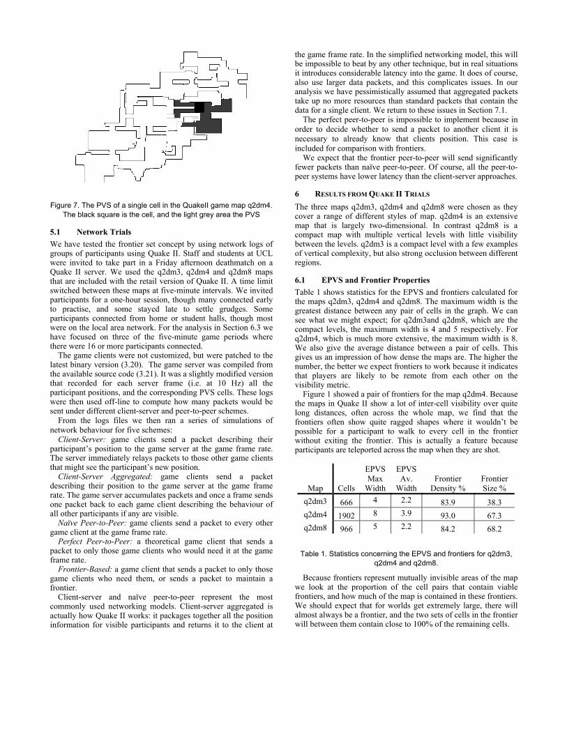
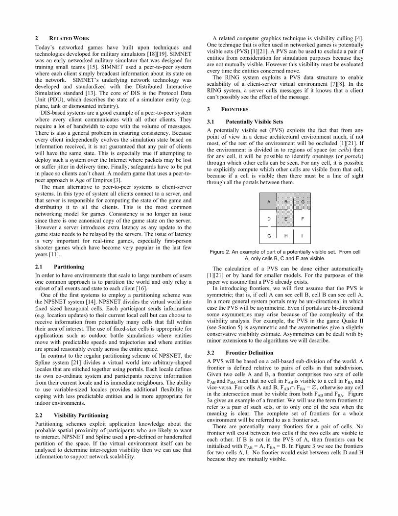
Figure 7. The PVS of a single cell in the QuakeII game map q2dm4. The black square is the cell, and the light grey area the PVS

5.1 Network Trials We have tested the frontier set concept by using network logs of groups of participants using Quake II. Staff and students at UCL were invited to take part in a Friday afternoon deathmatch on a Quake II server. We used the q2dm3, q2dm4 and q2dm8 maps that are included with the retail version of Quake II. A time limit switched between these maps at five-minute intervals. We invited participants for a one-hour session, though many connected early to practise, and some stayed late to settle grudges. Some participants connected from home or student halls, though most were on the local area network. For the analysis in Section 6.3 we have focused on three of the five-minute game periods where there were 16 or more participants connected.

The game clients were not customized, but were patched to the latest binary version (3.20). The game server was compiled from the available source code (3.21). It was a slightly modified version that recorded for each server frame (i.e. at 10 Hz) all the participant positions, and the corresponding PVS cells. These logs were then used off-line to compute how many packets would be sent under different client-server and peer-to-peer schemes.

From the logs files we then ran a series of simulations of network behaviour for five schemes:

Client-Server: game clients send a packet describing their participant’s position to the game server at the game frame rate. The server immediately relays packets to those other game clients that might see the participant’s new position.

Client-Server Aggregated: game clients send a packet describing their position to the game server at the game frame rate. The game server accumulates packets and once a frame sends one packet back to each game client describing the behaviour of all other participants if any are visible.

Naïve Peer-to-Peer: game clients send a packet to every other game client at the game frame rate.

Perfect Peer-to-Peer: a theoretical game client that sends a packet to only those game clients who would need it at the game frame rate.

Frontier-Based: a game client that sends a packet to only those game clients who need them, or sends a packet to maintain a frontier.

Client-server and naïve peer-to-peer represent the most commonly used networking models. Client-server aggregated is actually how Quake II works: it packages together all the position information for visible participants and returns it to the client at

the game frame rate. In the simplified networking model, this will be impossible to beat by any other technique, but in real situations it introduces considerable latency into the game. It does of course, also use larger data packets, and this complicates issues. In our analysis we have pessimistically assumed that aggregated packets take up no more resources than standard packets that contain the data for a single client. We return to these issues in Section 7.1.

The perfect peer-to-peer is impossible to implement because in order to decide whether to send a packet to another client it is necessary to already know that clients position. This case is included for comparison with frontiers.

We expect that the frontier peer-to-peer will send significantly fewer packets than naïve peer-to-peer. Of course, all the peer-to-peer systems have lower latency than the client-server approaches.

6 RESULTS FROM QUAKE II TRIALS The three maps q2dm3, q2dm4 and q2dm8 were chosen as they cover a range of different styles of map. q2dm4 is an extensive map that is largely two-dimensional. In contrast q2dm8 is a compact map with multiple vertical levels with little visibility between the levels. q2dm3 is a compact level with a few examples of vertical complexity, but also strong occlusion between different regions.

6.1 EPVS and Frontier Properties Table 1 shows statistics for the EPVS and frontiers calculated for the maps q2dm3, q2dm4 and q2dm8. The maximum width is the greatest distance between any pair of cells in the graph. We can see what we might expect; for q2dm3and q2dm8, which are the compact levels, the maximum width is 4 and 5 respectively. For q2dm4, which is much more extensive, the maximum width is 8. We also give the average distance between a pair of cells. This gives us an impression of how dense the maps are. The higher the number, the better we expect frontiers to work because it indicates that players are likely to be remote from each other on the visibility metric.

Figure 1 showed a pair of frontiers for the map q2dm4. Because the maps in Quake II show a lot of inter-cell visibility over quite long distances, often across the whole map, we find that the frontiers often show quite ragged shapes where it wouldn’t be possible for a participant to walk to every cell in the frontier without exiting the frontier. This is actually a feature because participants are teleported across the map when they are shot.

Map Cells

EPVS Max

Width

EPVS Av.

Width

Frontier

Density % Frontier Size %

q2dm3 666 4 2.2 83.9 38.3 q2dm4 1902 8 3.9 93.0 67.3 q2dm8 966 5 2.2 84.2 68.2

Table 1. Statistics concerning the EPVS and frontiers for q2dm3, q2dm4 and q2dm8.

Because frontiers represent mutually invisible areas of the map we look at the proportion of the cell pairs that contain viable frontiers, and how much of the map is contained in these frontiers. We should expect that for worlds get extremely large, there will almost always be a frontier, and the two sets of cells in the frontier will between them contain close to 100% of the remaining cells.

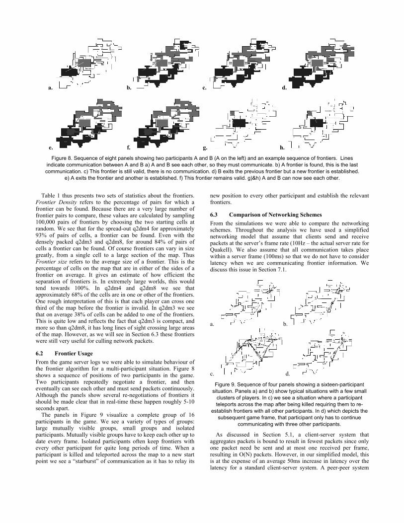
Table 1 thus presents two sets of statistics about the frontiers. Frontier Density refers to the percentage of pairs for which a frontier can be found. Because there are a very large number of frontier pairs to compare, these values are calculated by sampling 100,000 pairs of frontiers by choosing the two starting cells at random. We see that for the spread-out q2dm4 for approximately 93% of pairs of cells, a frontier can be found. Even with the densely packed q2dm3 and q2dm8, for around 84% of pairs of cells a frontier can be found. Of course frontiers can vary in size greatly, from a single cell to a large section of the map. Thus Frontier size refers to the average size of a frontier. This is the percentage of cells on the map that are in either of the sides of a frontier on average. It gives an estimate of how efficient the separation of frontiers is. In extremely large worlds, this would tend towards 100%. In q2dm4 and q2dm8 we see that approximately 68% of the cells are in one or other of the frontiers. One rough interpretation of this is that each player can cross one third of the map before the frontier is invalid. In q2dm3 we see that on average 38% of cells can be added to one of the frontiers. This is quite low and reflects the fact that q2dm3 is compact, and more so than q2dm8, it has long lines of sight crossing large areas of the map. However, as we will see in Section 6.3 these frontiers were still very useful for culling network packets.

6.2 Frontier Usage From the game server logs we were able to simulate behaviour of the frontier algorithm for a multi-participant situation. Figure 8 shows a sequence of positions of two participants in the game. Two participants repeatedly negotiate a frontier, and then eventually can see each other and must send packets continuously. Although the panels show several re-negotiations of frontiers it should be made clear that in real-time these happen roughly 5-10 seconds apart.

The panels in Figure 9 visualize a complete group of 16 participants in the game. We see a variety of types of groups: large mutually visible groups, small groups and isolated participants. Mutually visible groups have to keep each other up to date every frame. Isolated participants often keep frontiers with every other participant for quite long periods of time. When a participant is killed and teleported across the map to a new start point we see a “starburst” of communication as it has to relay its

new position to every other participant and establish the relevant frontiers.

6.3 Comparison of Networking Schemes From the simulations we were able to compare the networking schemes. Throughout the analysis we have used a simplified networking model that assume that clients send and receive packets at the server’s frame rate (10Hz – the actual server rate for QuakeII). We also assume that all communication takes place within a server frame (100ms) so that we do not have to consider latency when we are communicating frontier information. We discuss this issue in Section 7.1.

a. b.

c. d.

Figure 9. Sequence of four panels showing a sixteen-participant situation. Panels a) and b) show typical situations with a few small

clusters of players. In c) we see a situation where a participant teleports across the map after being killed requiring them to re-

establish frontiers with all other participants. In d) which depicts the subsequent game frame, that participant only has to continue

communicating with three other participants.

As discussed in Section 5.1, a client-server system that aggregates packets is bound to result in fewest packets since only one packet need be sent and at most one received per frame, resulting in O(N) packets. However, in our simplified model, this is at the expense of an average 50ms increase in latency over the latency for a standard client-server system. A peer-peer system

a. b. c. d.

e. f. g. h.

Figure 8. Sequence of eight panels showing two participants A and B (A on the left) and an example sequence of frontiers. Lines indicate communication between A and B a) A and B see each other, so they must communicate. b) A frontier is found, this is the last communication. c) This frontier is still valid, there is no communication. d) B exits the previous frontier but a new frontier is established.

e) A exits the frontier and another is established. f) This frontier remains valid. g)&h) A and B can now see each other.

with no scalability must send and receive O(N2) packets a second, but the latency is low.

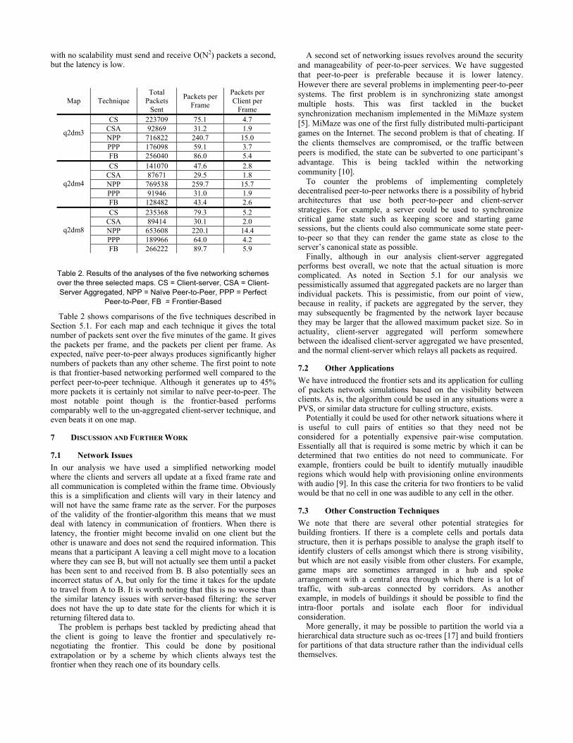
Map Technique Total

Packets Sent

Packets per Frame

Packets per Client per

Frame CS 223709 75.1 4.7

CSA 92869 31.2 1.9 NPP 716822 240.7 15.0 PPP 176098 59.1 3.7

q2dm3

FB 256040 86.0 5.4 CS 141070 47.6 2.8

CSA 87671 29.5 1.8 NPP 769538 259.7 15.7 PPP 91946 31.0 1.9

q2dm4

FB 128482 43.4 2.6 CS 235368 79.3 5.2

CSA 89414 30.1 2.0 NPP 653608 220.1 14.4 PPP 189966 64.0 4.2

q2dm8

FB 266222 89.7 5.9

Table 2. Results of the analyses of the five networking schemes over the three selected maps. CS = Client-server, CSA = Client-Server Aggregated, NPP = Naïve Peer-to-Peer, PPP = Perfect

Peer-to-Peer, FB = Frontier-Based

Table 2 shows comparisons of the five techniques described in Section 5.1. For each map and each technique it gives the total number of packets sent over the five minutes of the game. It gives the packets per frame, and the packets per client per frame. As expected, naïve peer-to-peer always produces significantly higher numbers of packets than any other scheme. The first point to note is that frontier-based networking performed well compared to the perfect peer-to-peer technique. Although it generates up to 45% more packets it is certainly not similar to naïve peer-to-peer. The most notable point though is the frontier-based performs comparably well to the un-aggregated client-server technique, and even beats it on one map.

7 DISCUSSION AND FURTHER WORK

7.1 Network Issues In our analysis we have used a simplified networking model where the clients and servers all update at a fixed frame rate and all communication is completed within the frame time. Obviously this is a simplification and clients will vary in their latency and will not have the same frame rate as the server. For the purposes of the validity of the frontier-algorithm this means that we must deal with latency in communication of frontiers. When there is latency, the frontier might become invalid on one client but the other is unaware and does not send the required information. This means that a participant A leaving a cell might move to a location where they can see B, but will not actually see them until a packet has been sent to and received from B. B also potentially sees an incorrect status of A, but only for the time it takes for the update to travel from A to B. It is worth noting that this is no worse than the similar latency issues with server-based filtering: the server does not have the up to date state for the clients for which it is returning filtered data to.

The problem is perhaps best tackled by predicting ahead that the client is going to leave the frontier and speculatively re-negotiating the frontier. This could be done by positional extrapolation or by a scheme by which clients always test the frontier when they reach one of its boundary cells.

A second set of networking issues revolves around the security and manageability of peer-to-peer services. We have suggested that peer-to-peer is preferable because it is lower latency. However there are several problems in implementing peer-to-peer systems. The first problem is in synchronizing state amongst multiple hosts. This was first tackled in the bucket synchronization mechanism implemented in the MiMaze system [5]. MiMaze was one of the first fully distributed multi-participant games on the Internet. The second problem is that of cheating. If the clients themselves are compromised, or the traffic between peers is modified, the state can be subverted to one participant’s advantage. This is being tackled within the networking community [10].

To counter the problems of implementing completely decentralised peer-to-peer networks there is a possibility of hybrid architectures that use both peer-to-peer and client-server strategies. For example, a server could be used to synchronize critical game state such as keeping score and starting game sessions, but the clients could also communicate some state peer-to-peer so that they can render the game state as close to the server’s canonical state as possible.

Finally, although in our analysis client-server aggregated performs best overall, we note that the actual situation is more complicated. As noted in Section 5.1 for our analysis we pessimistically assumed that aggregated packets are no larger than individual packets. This is pessimistic, from our point of view, because in reality, if packets are aggregated by the server, they may subsequently be fragmented by the network layer because they may be larger that the allowed maximum packet size. So in actuality, client-server aggregated will perform somewhere between the idealised client-server aggregated we have presented, and the normal client-server which relays all packets as required.

7.2 Other Applications We have introduced the frontier sets and its application for culling of packets network simulations based on the visibility between clients. As is, the algorithm could be used in any situations were a PVS, or similar data structure for culling structure, exists.

Potentially it could be used for other network situations where it is useful to cull pairs of entities so that they need not be considered for a potentially expensive pair-wise computation. Essentially all that is required is some metric by which it can be determined that two entities do not need to communicate. For example, frontiers could be built to identify mutually inaudible regions which would help with provisioning online environments with audio [9]. In this case the criteria for two frontiers to be valid would be that no cell in one was audible to any cell in the other.

7.3 Other Construction Techniques We note that there are several other potential strategies for building frontiers. If there is a complete cells and portals data structure, then it is perhaps possible to analyse the graph itself to identify clusters of cells amongst which there is strong visibility, but which are not easily visible from other clusters. For example, game maps are sometimes arranged in a hub and spoke arrangement with a central area through which there is a lot of traffic, with sub-areas connected by corridors. As another example, in models of buildings it should be possible to find the intra-floor portals and isolate each floor for individual consideration.

More generally, it may be possible to partition the world via a hierarchical data structure such as oc-trees [17] and build frontiers for partitions of that data structure rather than the individual cells themselves.

Finally we note that if a cell C is in a frontier FAB, then it is likely that cell A would be in FCB. Thus instead of starting from scratch for each pair, it may be possible to re-use a frontier and adapt it by removing conflicting cells and adding others.

8 CONCLUSIONS We have introduced frontier sets: a simple but powerful visibility structure and we have shown how they can be constructed at run-time. For a pair of nodes, a frontier identifies two regions of mutual invisibility containing those nodes. For any application where there is a need to cope with a large number of entities in a space that lends itself to spatial partitioning, frontiers should be a useful extension to enable scalability.

We have demonstrated the use of frontiers in simulations of the networked game Quake II. Networked games are a good example of a problem that involves multiple entities, all of which can potentially interact. This leads to an O(N2) simulation problem. Fortunately network games often exhibit spatial separation of participants, so that we can usually discount many pairs of participants from potentially expensive operations such as communication of network state. We demonstrated that a network protocol based on frontiers has performance close to a client-server system and close to an ideal model of peer-to-peer systems. An aggregated client-server system is still faster than frontier-based system, but to counter this, frontier-based has a significantly lower latency of communication. Using frontiers it should be possible to build a peer-to-peer game that scales more efficiently than existing peer-to-peer systems.

In order to build frontier sets at run-time, we pre-computed an enhanced potentially visible set which only requires O(N2) space in the number of cells. Since many games already require a PVS with this space requirement, this means that there is very little space overhead from using frontiers.

In our current work we are planning to apply frontiers to other simulation situations. We are also attempting to build a peer-to-peer version of Quake II.

ACKNOWLEDGEMENTS All the code modifications we made to the GPL Quake II source code will be available from http://www.cs.ucl.ac.uk/research/vr/. This work was supported in part by the UK Equator project (EPSRC Grant GR/N15986/01).

REFERENCES [1] AIREY, E.J. M., ROHLF, J. H. AND BROOKS Jr. F.P.

1990. Towards image realism with interactive update rates in complex virtual building environments. Computer Graphics (Proceedings of ACM Symposium on Interactive 3D Graphics), 24(2): 41—50.

[2] BAUER, D., ROONEY, S. AND SCOTTON, P. 2002. Network Infrastructure for Massively Distributed Games. In NetGames 2002, April 16-17, Braunschweig, Germany, ACM.

[3] BETTNER, P. AND TERRANO, M. 2001. 1500 Archers on a 29.8: Networking Programming in Age of Empires and Beyond. In The 2001 Game Developer Conference Proceedings, San Jose, CA, Mar. 2001.

[4] COHEN-OR, D., CHRYSANTHOU, Y., SILVA, C. AND DURANT, F. 2003. A Survey of Visibility for Walk-through Applications. IEEE Transactions on Visualization and Computer Graphics, 9(3): 412-431.

[5] Diot, C. and Gautier, L. 1999. A Distributed Architecture for MultiParticipant Interactive Applications on the Internet. In IEEE Network, 13(4), 6-15.

[6] FUCHS, H., KEDEM Z.M. AND NAYLOR. B.F. 1980. On Visible Surface Generation by A Priori Tree Structures. In

Computer Graphics (Proceedings of ACM SIGGRAPH 80), 14(3), ACM, 124-133.

[7] FUNKHOUSER, T. A. 1995. RING: A Client-Server System for Multi-User Virtual Environments. In 1995 Symposium on Interactive 3D Graphics. 85-92, April 1995.

[8] FUNKHOUSER, T. A. 1996. Network Topologies for Scalable Multi-User Virtual Environments. In Proceedings IEEE VRAIS ‘96, San Jose, CA, April, 1996.

[9] FUNKHOUSER, T.A., MIN, P. AND CARLBOM, I. 1999. Real-Time Acoustic Modeling for Distributed Virtual Environments. In Proceedings of ACM SIGGRAPH 1999, ACM Press / ACM SIGGRAPH, New York. A. Rockwoord, Ed., Computer Graphics Proceedings, Annual Conference Series, ACM, 365-374.

[10] GAUTHIERDICKEY, C., ZAPPALA, D., LO, V. AND MARR, J. 2003, Cheat-Proof Event Ordering for Peer-to-Peer Games. Draft paper, http://www.cs.uoregon.edu/~zappala

[11] HENDERSON, T. 2001. Latency and User Behaviour on a Multiparticipant Game Server. Networked Group Communication 2001, Third International COST264 Workshop, London, UK, November 7-9, 2001 1-13

[12] IDSOFTWARE. 1997. Quake II. http://www.idsoftware.com/games/quake/quake2/

[13] IEEE. 1993. ANSI/IEEE Standard 1278-1993, Standard for Information Technology, Protocols for Distributed Interactive Simulation, March 1993.

[14] MACEDONIA, M. R., ZYDA, M. J., PRATT, D. R., BARHAM, P. T., ZESWITZ, S. 1994. NPSNET: A Network Software Architecture for Large Scale Virtual Environments. Presence: Teleoperators and Virtual Environments, 3(4): 265-287, MIT Press.

[15] MILLER, D., AND THORPE, J. 1995. SIMNET: the advent of simulator networking. Proceedings of IEEE, 83(8): 1114-1123.

[16] MORSE, K. L., BIC, L. AND DILLENCOURT, M. 2000. Interest management in large-scale virtual environments. Presence: Teleoperators and Virtual Environments, 9(1):52--68, MIT Press.

[17] SAMET. H. 1989. Spatial Data Structures: Quadtree, Octrees and Other Hierarchical Methods. Addison Wesley.

[18] SINGHAL, S. ZYDA, M. 1999. Networked Virtual Environments: Design and Implementation. Addison-Wesley.

[19] SMED, J. KAUKORANTA, T. AND HAKONEN, H. 2001. Aspects of Networking in Multiparticipant Computer Games. In Loo Wai Sing, Wan Hak Man, and Wong Wai (eds.), Proceedings of International Conference on Application and Development of Computer Games in the 21st Century. Hong Kong SAR, China, Nov. 2001, 74-81.

[20] STEED, A. AND ANGUS, C. 2004, Frontier Sets: A Partitioning Scheme to Enable Scalable Virtual Environments, To be presented at Eurographics 2004 (Short Paper Presentation).

[21] STERNS, I.B. AND YERAZUNIS, W.S. 1997. Diamond Park and Spline: Social Virtual Reality with 3D Animation, Spoken Interaction and Runtime Extendability. Presence: Teleoperators and Virtual Environments, 6(4), 461-481, MIT Press

[22] TELLER, S.J. AND SEQUIN, C.H. 1991. Visibility Preprocessing for interactive walkthroughs. Computer Graphics (Proceedings of SIGGRAPH 91), 25(4):61-90.

[23] VAN DE PANNE, M. AND STEWART, A. J. 1999. Effective compression techniques for precomputed visibility. In Proc. Eurographics Rendering Workshop, June 1999, 305-316.