Supporting InformationCrawford et al. 10.1073/pnas.0914115107SI Materials and MethodsField Data. To test for a significant change in community-wideabundance inpre- versuspostdeclineperiods,werana linearmixed-effects repeated-measures ANOVA on the 53 species with quan-titative abundance data (Table S2), designating species as a ran-dom effect and survey date as a fixed effect variable. Analyses wereconducted in the statistical environment R (1) using the functionlme in the nlme package to account for nonindependence of ob-servations. To individually test each of the 53 species for a changein abundance in predecline versus postdecline surveys, we applieda nonparametric Wilcoxon rank-sum test with continuity correc-tion. We did not apply a Bonferroni correction for multiple testsas, with a sample size of six field seasons, adopting an α value of0.001 would leave no power to reject the null hypothesis. Thesesingle-species tests serve to highlight taxa of interest, but the sig-nificance levels should be interpreted with caution.

Genetic Data. Most genetic samples were collected before thedecline event (2), with some additional material collected fromdead frogs in November 2004, most notably the samples of Ate-lopus zeteki. Twenty samples came from toe clips and 280 samplescame from vouchered specimens (Table S3). For three species(Oedipina collaris, Oophaga vicente, and Ranitomeya minuta), weused previously published data obtained from samples collectedduring our field surveys (Table S3). For another three species, weused samples collected elsewhere in Panama: Bolitoglossa co-lonnea, Oedipina parvipes, and Dendrobates auratus. These threesubstitutions should not affect our estimates of PD as long asintraspecific variation is low relative to interspecific divergence.GenomicDNAwas extractedwith a standard phenol-choloform

protocol implemented with an AutoGenprep 965 (AutoGen)automated DNA isolation robot following digestion with pro-teinase K (0.4 mg/mL) at 55 °C. After a maximum of three at-tempts, the 16S primers yielded a failure rate of 1.3% and thedegenerate COI primers failed in 7.7% of samples, which is lowerthan the failure rate reported previously in amphibian barcodesurveys (3, 4). All COI and 16S sequences were deposited inBoLD (http://www.barcodinglife.com) and GenBank (Table S3).The concatenated two-gene DNA sequence alignment (includinginferred gaps) was submitted to TreeBASE (www.treebase.org)under study accession number S2643.The COI sequences were 648 bp long and showed no length

variation. The 16S gene fragments were aligned with defaultparameters andmultiple iterations inClustalX2.0 (5).All analysesof the 16S data excluded sites with gaps plus one additional baseon either side of all gaps of length greater than 1 bp, resulting in436 aligned bp included in phylogenetic and distance analyses.

Phylogenetic Analyses. We inferred an unconstrained molecularphylogeny by Metropolis coupled Markov chain Monte Carlo(MCMC) Bayesian analysis (6, 7) using a parallel version ofMrBayes 3.1.2 (8, 9). Selection of appropriate models of nucle-otide substitution used a Bayesian information criterion as im-plemented inDT-ModSel (10) andModeltest 3.7 (11), which gaveidentical results. Four data partitions were created: 16S plus co-don positions 1 through 3 in COI, with the following models ap-plied to each GTR+I+Γ, GTR+I, GTR+Γ, and GTR+I+Γ, re-spectively (12–14). Rates of evolution were allowed to vary acrosspartitions using a rate multiplier (15). Each analysis consisted ofthree parallel MCMC runs with three Metropolis-coupled chainseach. Two initial analyses of 2 million generations each wereconducted, and prior distributions, the heating parameter, and

burn-in were adjusted according. Our final analysis consisted of 8million generations with trees sampled every 2,000 generations,a burn-in period of 2 million generations (at which point the av-erage SD of split frequencies had decreased to less than 0.032),heating parameter of 0.01 (resulting frequencies of chain swap-ping ranged from 0.07 to 0.73), a U (0.0001, 20.0) prior distribu-tion on shape parameters, and an exponential (5.0) priordistribution of branch lengths. Bayesian consensus tree with nodalsupport and unmodified branch lengths is shown in Fig. S2.We also inferred a molecular phylogeny constrained to match

published higher level amphibian relationships using unpartitionedML analysis (16) implemented in the software, GARLI, version0.95 (17), run six times assuming a single GTR+I+Γ model anddefault parameters except that the setting of generations withoutimproving topology was increased to 50,000. TheML treematchedthe Bayesian tree at all well-supported nodes. Both trees largelyagreed with previously published higher level amphibian rela-tionships, with five exceptions that were constrained in theGARLIanalyses: monophyletic Bufonidae, monophyletic Hylidae, Lep-todactylidae + Leiuperidae (18), ((Strabomantidae) (Craugas-toridae) Eleutherodactylidae (19), and within Bufonidae the clade((Rhinella, Incilius)Rhaebo) (20). Because of the lack of resolutioneven with manymore genes, no other relationships among familieswithin Hyloidea were constrained in the GARLI analyses. Thefollowing relationships were also constrained in the GARLI anal-yses, yet were successfully recovered in the unconstrained Bayesianphylogenetic analyses (Fig. S2). Within Craugastor: theC. fitzingerigroup, C. gollmeri group, and the C. rugulosus group + C. bi-porcatus group (21, 22); all genera monophyletic; within Phyllo-medusinae, ((Agalychnis, Hylomantis) Cruziohyla) (23); theCentral America Hylinae, Ecnomiohyla+ Smilisca (24); the SouthAmerican Hylinae, Hyloscirtus + Hypsiboas (25); monophyleticHylinae (25); within Dendrobatidae, ((Oophaga, Dendrobates)(Ranitomeya) Phyllobates) and Silverstoneia + Colostethus (26);within Centrolenidae, Hyalinobatrachium sister to all other cen-trolenids sampled here (27); monophyletic Hemiphractidae (27);Microhylidae + Ranidae (18); Aromobatidae + Dendrobatidae(26); as well as a monophyletic Caudata, Anura, and Batrachia(Caudata + Anura).

Candidate Species. We emphasize that the candidate species des-ignation is provisional, pending further systematic investigations(28), and that evolutionary processes such as introgression, re-tentionof ancestral polymorphisms, and rapid speciationmay causeincongruence between mitochondrial DNA gene trees and speciesboundaries (29). Although threshold values of more than 8% inCOI and more than 2% at 16S (Fig. 1 in the main text) are lowerthan has been suggested previously in the literature (30), they weredetermined empirically for the present dataset via an analysis ofa bivariate barcode gap (Fig. 1 in the main text). Divergence at 16Smay have been underestimated if the same sites that contained in-formative point mutations distinguishing congeneric samples werethe same sites inferred to contain gapswhenwealigned families andorders of amphibians (as describedearlier). Such sites could includethe more variable loop regions of the 16S rRNA molecule (4).Three species (O. collaris, Diasporus quidditus, and D. aff. di-

astema) lacked COI data (Table S3). These lineages showed 5.4%to 7.7% mean K2P divergence from their nearest relative (Fig. 2)at the 16S gene, placing D. aff. diastema as well asD. aff. quidditusin the category of candidate species relative toD. quidditus. Recentstudies have found that the DNA barcoding gap may not be sig-nificantly influenced by the number of individuals sequenced per

Crawford et al. www.pnas.org/cgi/content/short/0914115107 1 of 5

species (31). In this study, total sample size (N) for some pairs ofnamed plus candidate species was low, yet these pairs showed highK2P percent divergence at COI:Cruziohyla calcariferA+B (n=3)showed 12.5% divergence, Lithobates warszewitschii + L. aff.warszewitschii (n=4) showed 14.7%, Pristimantis ridensA+B (n=4) showed 17.6%, and P. caryophyllaceus A+B+C (n = 7) 14.5%.These levels of mtDNA variation are higher than the maximumpolymorphism observed for sympatric samples of conspecific am-phibians (32, 33). Thus, sympatry provides additional evidence thatthese named taxa include candidate species (34).

Loss of Evolutionary History. Because we used relatively fast-evolvingmitochondrial DNAmarkers to infer the history of an oldgroup of vertebrates, the lengths of basal branches may beunderestimated. To investigate the affect of basal branch lengthvariation, we also estimated the loss of PD on a tree temporallycalibrated (aswell as topologically constrained; as detailed earlier)on the basis of a molecular analysis of lissamphibian evolutionaryhistory (18). The divergence times assumed here may be too old(35), but any bias toward older ages should provide a sharperpotential contrast in the loss of PD between trees with longer(time-calibrated) versus shorter (noncalibrated) basal branches.We imposed the following temporal constraints on our phylogenyusing the MPL algorithm. We set the age of the most recentcommon ancestor (MRCA) of Lissamphibia at 332.6million yearsago (Ma), theminimum age of Batrachia (18).We constrained theminimum and maximum ages of three nested nodes, as follows:the MRCA of Craugastor + Lithobates (Phtanobatrachia) to theinterval 143.3 to 179.9 Ma, the MRCA of Lithobates + Nelsono-phryne (Ranoidea) to the interval 106.2 to 130.9 Ma, and theMRCA of Craugastor + Rhinella (Nobleobatrachia minus

Rhinoderma) to the interval 50.9 to 75.5 Ma (18). The resultingtree had much longer basal branch lengths, yet the resulting cal-culations of PD lost were very similar to those obtained for theMPL tree (Table 1), suggesting that our results were robust tosubstantial variation in branch lengths.

Trait Evolution. In testing for a phylogenetic correlation of percentdecline in abundance among species, trait values were coded al-ternatively as percent change in abundance (Table S2) or asa percent decline (as a positive value) such that increases inabundance were coded as 0% decline. The GLS model describesthe covariance of trait values and phylogeny, and assumes anevolutionary parameter, λ, for which a value of 0.0 indicates traitvalues are independent of shared history, whereas a value of 1.0implies that trait evolution conforms to a randomwalk on the givenphylogeny. Because abundance is a species-level trait, analyseswere conducted on phylogenies containing one sample per each ofthe 74 named or candidate species. For Bayesian analyses, the 100unconstrained trees were sampled at a rate of one tree per 10,000generations from the final third of a BayesianMCMCphylogeneticanalysis run for 3 million generations in MrBayes. Conditions for74-sample phylogenetic analyses were otherwise the same as for300-sample analyses as described earlier. Time series plots of log-likelihood scores and SDs of among-chain split frequencies lowerthan 0.03 suggested convergence was reach by each independentchain. Using the software BayesTraits, the marginal likelihoods ofλ under alternative models were approximated from a MCMCanalysis run for 1 million generations preceding by a 50,000 gen-eration burn-in period, with parameter values recorded once per300 generations. At each generation, one of the 100 trees was se-lected at random and proposed λ values were evaluated.

1. R Development Core Team (2008) R: A Language and Environment for StatisticalComputing. (R Foundation, Vienna).

2. Lips KR, et al. (2006) Emerging infectious disease and the loss of biodiversity ina Neotropical amphibian community. Proc Natl Acad Sci USA 103:3165–3170.

3. Smith MA, Poyarkov NA, Jr, Hebert PDN (2008) CO1 DNA barcoding amphibians: Takethe chance, meet the challenge. Mol Ecol Notes 8:235–246.

4. Vences M, Thomas M, van der Meijden A, Chiari Y, Vieites DR (2005) Comparativeperformance of the 16S rRNA gene in DNA barcoding of amphibians. Front Zool 2:5.

5. Thompson JD, Gibson TJ, Plewniak F, Jeanmougin F, Higgins DG (1997) TheCLUSTAL_X windows interface: Flexible strategies for multiple sequence alignmentaided by quality analysis tools. Nucleic Acids Res 25:4876–4882.

6. Yang Z, Rannala B (1997) Bayesian phylogenetic inference using DNA sequences: AMarkov Chain Monte Carlo Method. Mol Biol Evol 14:717–724.

7. Rannala B, Yang Z (1996) Probability distribution of molecular evolutionary trees:a new method of phylogenetic inference. J Mol Evol 43:304–311.

8. Altekar G, Dwarkadas S, Huelsenbeck JP, Ronquist F (2004) Parallel Metropolis coupledMarkov chainMonteCarlo forBayesianphylogenetic inference.Bioinformatics20:407–415.

9. Ronquist F, Huelsenbeck JP (2003) MrBayes 3: Bayesian phylogenetic inference undermixed models. Bioinformatics 19:1572–1574.

10. Minin V, Abdo Z, Joyce P, Sullivan J (2003) Performance-based selection of likelihoodmodels for phylogeny estimation. Syst Biol 52:674–683.

11. Posada D, Crandall KA (1998) MODELTEST: Testing the model of DNA substitution.Bioinformatics 14:817–818.

12. Hasegawa M, Kishino H, Yano T (1987) Man’s place in Hominoidea as inferred frommolecular clocks of DNA. J Mol Evol 26:132–147.

13. Yang Z (1994) Maximum likelihood phylogenetic estimation from DNA sequenceswith variable rates over sites: Approximate methods. J Mol Evol 39:306–314.

14. Tavaré S (1986) Some probabilistic and statistical problems on the analysis of DNAsequences. Lect Math Life Sci 17:57–86.

15. Marshall DC, Simon C, Buckley TR (2006) Accurate branch length estimation inpartitioned Bayesian analyses requires accommodation of among-partition ratevariation and attention to branch length priors. Syst Biol 55:993–1003.

16. Felsenstein J (1981) Evolutionary trees from DNA sequences: A maximum likelihoodapproach. J Mol Evol 17:368–376.

17. Zwickl DJ (2006) Genetic algorithm approaches for the phylogenetic analysis of largebiological sequence datasets under the maximum likelihood criterion. PhD dissertation(Univ of Texas, Austin).

18. Roelants K, et al. (2007) Global patterns of diversification in the history of modernamphibians. Proc Natl Acad Sci USA 104:887–892.

19. HeinickeMP,etal. (2009)Anewfrogfamily (Anura:Terrarana) fromSouthAmericaandanexpanded direct-developing clade revealed bymolecular phylogeny. Zootaxa 2211:1–35.

20. Van Bocxlaer I, Biju SD, Loader SP, Bossuyt F (2009) Toad radiation reveals into-Indiadispersal as a source of endemism in the Western Ghats-Sri Lanka biodiversityhotspot. BMC Evol Biol 9:131.

21. Heinicke MP, Duellman WE, Hedges SB (2007) Major Caribbean and Central Americanfrog faunas originated by ancient oceanic dispersal. Proc Natl Acad Sci USA 104:10092–10097.

22. Crawford AJ, Smith EN (2005) Cenozoic biogeography and evolution in direct-developing frogs of Central America (Leptodactylidae: Eleutherodactylus) as inferredfrom a phylogenetic analysis of nuclear and mitochondrial genes. Mol PhylogenetEvol 35:536–555.

23. Faivovich J, et al. (2009) The phylogenetic relationships of the charismatic posterfrogs, Phyllomedusinae (Anura, Hylidae). Cladistics 26:227–261.

24. Smith SA, de Oca AN, Reeder TW, Wiens JJ (2007) A phylogenetic perspective onelevational species richness patterns in Middle American treefrogs: Why so fewspecies in lowland tropical rainforests? Evolution 61:1188–1207.

25. Wiens JJ, Graham CH, Moen DS, Smith SA, Reeder TW (2006) Evolutionary andecological causes of the latitudinal diversity gradient in hylid frogs: Treefrog treesunearth the roots of high tropical diversity. Am Nat 168:579–596.

26. Santos JC, et al. (2009) Amazonian amphibian diversity is primarily derived from lateMiocene Andean lineages. PLoS Biol 7:e56.

27. Guayasamin JM, Castroviejo-Fisher S, Ayarzagüena J, Trueb L, Vilà C (2008)Phylogenetic relationships of glassfrogs (Centrolenidae) based on mitochondrial andnuclear genes. Mol Phylogenet Evol 48:574–595.

28. Vieites DR, et al. (2009) Vast underestimation of Madagascar’s biodiversityevidenced by an integrative amphibian inventory. Proc Natl Acad Sci USA 106:8267–8272.

29. Moritz C, Cicero C (2004) DNA barcoding: Promise and pitfalls. PLoS Biol 2:e354.30. Fouquet A, et al. (2007) Underestimation of species richness in neotropical frogs

revealed by mtDNA analyses. PLoS ONE 2:e1109.31. Aliabadian M, Kaboli M, Nijman V, Vences M (2009) Molecular identification of birds:

Performance of distance-based DNA barcoding in three genes to delimit parapatricspecies. PLoS ONE 4:e4119.

32. CrawfordAJ (2003)Hugepopulationsandold speciesofCostaRicanandPanamaniandirtfrogs inferred frommitochondrial and nuclear gene sequences.Mol Ecol 12:2525–2540.

33. Vences M, Thomas M, Bonett RM, Vieites DR (2005) Deciphering amphibian diversitythrough DNA barcoding: Chances and challenges. Philos Trans R Soc Lond B Biol Sci360:1859–1868.

34. Mallet J (2008) Hybridization, ecological races and the nature of species: Empiricalevidence for the ease of speciation. Philos Trans R Soc Lond B Biol Sci 363:2971–2986.

35. Marjanović D, Laurin M (2007) Fossils, molecules, divergence times, and the origin oflissamphibians. Syst Biol 56:369–388.

36. Pounds JA, Fogden MPL, Campbell JH (1999) Biological response to climate change ona tropical mountain. Nature 398:611–615.

37. Lips KR (1999) Mass mortality and population declines of anurans at an upland site inwestern Panama. Conserv Biol 13:117–125.

38. Lips KR (1998) Decline of a tropical montane amphibian fauna. Conserv Biol 12:106–117.

Crawford et al. www.pnas.org/cgi/content/short/0914115107 2 of 5

Fig. S1. Bimodal distribution of percent decline in abundance among the 74 known and candidate species of the El Copé study site. We defined the followingconservation categories on the basis of this distribution. Extirpated species were regularly seen on predecline transects but never on postdecline transects.Critical species declined by 85% to 99% in abundance. Declined species were reduced by 1% to 55%. Least concern species experienced a positive (+) change inabundance on postdecline transects. Thus, percent change in abundance for pre- versus postdecline transects shows a natural break, with species either im-pacted greatly (extirpated or critical) or relatively little (declined or least concern). Eighteen named species plus one candidate species (Cruziohyla calcarifer B)lacked sufficient field data to calculate percent change and were classified as DD and counted as either DD–least concern (10 species) or DD–extirpated (ninespecies) on the basis of how these species have responded to the presence of B. dendrobatidis at other sites (36–38).

Crawford et al. www.pnas.org/cgi/content/short/0914115107 3 of 5

Fig. S2. Bayesian 50% majority rule consensus phylogeny showing statistical support for nodes and the distribution of percent of decline. Topology andbranch lengths were unconstrained (unlike Fig. 2 in the main text). Nodes with marginal posterior probability of 0.95–1.0 are indicated by a white dot. Percentdecline constrained to positive values 0–100 is indicated by color (see legend). Ancestral states were inferred using least-squares parsimony with the software,Mesquite (1).

1. Maddison WP, Maddison DR (2009) Mesquite: a modular system for evolutionary análisis, Version 2.6. Available at http://mesquiteproject.org.

Crawford et al. www.pnas.org/cgi/content/short/0914115107 4 of 5

Table S1. Field effort on standardized transects during each fieldseason, plus predecline and postdecline totals, used to calculaterelative abundances

Field effort on standardized transects during each field season, plus prede-cline and postdecline totals, used to calculate relative abundances (Table S2).Field effort is given as number of individual amphibians captured, numberof surveys conducted, mean number of captures per survey, total numberof hours invested, and total number of kilometers walked during a given in-terval. Number of species captured includes species found off of standardizedtransects.

Table S1

Table S2. Mean, SD, minimum, and maximum yearly abundancefor predecline and postdecline periods, followed by percentchange in abundance of each species and the resulting categoryof decline

Relative abundance was calculated as total number of captures per kilo-meter of survey during each field season, then averaged across seasons togive predecline and postdecline mean relative abundances. “Pond” refers topond-breeding species that were abundant in local ponds that were notsituated on standardized transects. “Rare” refers to additional species cap-tured in the area but not during standardized surveys. “Candidate” refers tocandidate species discovered by genetic analyses (4 candidate species wereregarded as morphospecies in the field and abundance data were collected).Declines that were significant according to a nonparametric test (α = 0.05,without Bonferroni correction) are indicated with an asterisk. See Materialsand Methods for details.

Table S2

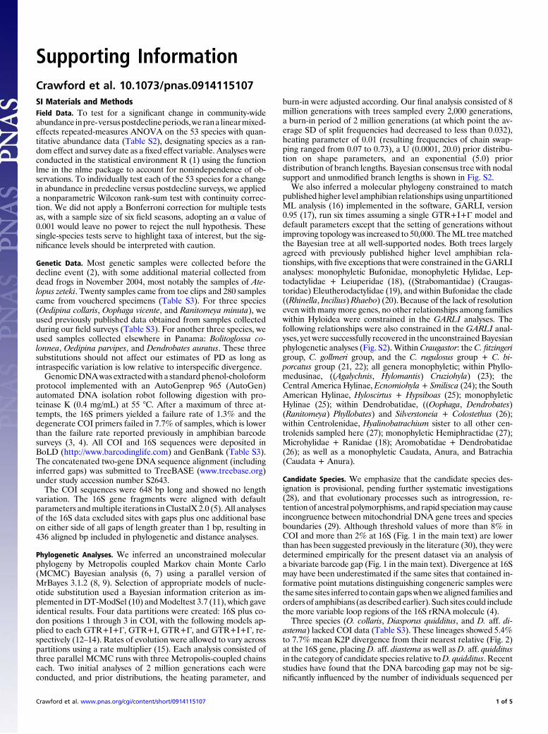
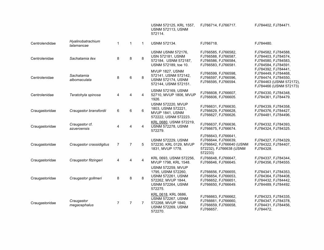
Table S3. Number of DNA sequences from COI and 16S genesobtained per named and candidate species, sample numbers,and corresponding GenBank numbers

Taxonomy follows recently suggested changes (ref. 27 and http://research.amnh.org/herpetology/amphibia). The two non-anuran families are indicatedin bold. Within each species, sample numbers are given in the same order astheir corresponding GenBank numbers, except sample numbers for single-gene data are in parentheses following the corresponding GenBank number.USNM, specimen voucher number in the National Museum of Natural History,Smithsonian Institution,Washington, DC;MVUP, specimen voucher number inthe Museo de Vertebrados de la Universidad de Panamá, Republic of Panama;CH, specimen voucher number in the Círculo Herpetológico de Panamá, Re-public of Panama; KRL andAJC, authors’ field numbers for specimens awaitingaccession numbers; toe, genetic data obtained from toe clip (no voucheredspecimen). Specimens with underlined KRL numbers were used for histopath-ological study and are no longer available.

Table S3

Crawford et al. www.pnas.org/cgi/content/short/0914115107 5 of 5

Table S1. Field effort on standardized transects during each field season, plus predecline and postdecline totals, used to calculate relative abundances. Field effort on standardized transects during each field season, plus predecline and postdecline totals, used to calculate relative abundances (Table S2). Field effort is given as number of individual amphibians captured, number of surveys conducted, mean number of captures per survey, total number of hours invested, and total number of kilometers walked during a given interval. Number of species captured includes species found off of standardized transects.

Year

no.

captures no. species

no.

surveys

mean no.

captures /

survey no. hours no. km

2000 2,155 49 82 26.28 153.9 23.43

2001 3,523 54 92 38.29 180.5 25.13

2002 8,726 45 115 75.87 229.1 31.74

2003 6,763 52 112 60.38 198.8 32.48

pre-decline

totals 23,322 63 401 762.3 112.78

2006-2007 951 48 289 3.29 211.4 66.4

2008 95 29 9 10.55 10.3 2.7

post-

decline

totals

1,046 48 298 221.7 69.1

Table S2. Mean, SD, minimum, and maximum yearly abundance for predecline and postdecline periods, followed by percent change in abundance of each species and the resulting category of decline. Relative abundance was calculated as total number of captures per kilometer of survey during each field season, then averaged across seasons to give predecline and postdecline mean relative abundances. “Pond” refers to pond-breeding species that were abundant in local ponds that were not situated on standardized transects. “Rare” refers to additional species captured in the area but not during standardized surveys. “Candidate” refers to candidate species discovered by genetic analyses (4 candidate species were regarded as morphospecies in the field and abundance data were collected). Declines that were significant according to a nonparametric test (α = 0.05, without Bonferroni correction) are indicated with an asterisk. See Materials and Methods for details.

PRE-DECLINE POST-DECLINE

Family Taxon

Mea

n ab

unda

nce

Stan

dard

de

viat

ion

of

abun

danc

e

Min

imum

-M

axim

um

abun

danc

e

Mea

n ab

unda

nce

Stan

dard

de

viat

ion

of

abun

danc

e

Min

imum

-M

axim

um

abun

danc

e

% C

hang

e ab

unda

nce

Dec

line

cate

gory

Aromobatidae Allobates talamancae 0.0029 0.0037 0 - 0.0082 0.0000 0 0 - 0 -100 Extirpated Bufonidae Atelopus zeteki 0.1879 0.2918 0.0362 - 0.6255 0.0218 0.0309 0 - 0.0437 -88.38 Critical Bufonidae Incilius coniferus 0.0366 0.0689 0.0016 - 0.1399 0.0428 0.0077 0.0373- 0.0482 16.86 LC Bufonidae Rhaebo haematiticus 0.0230 0.0286 0.0068 - 0.0658 0.0023 0.0032 0 - 0.0045 -90.17* Critical Bufonidae Rhinella marina pond 0 DD-LC Caecilidae Caecilia volcani rare 0 DD-LC Centrolenidae Cochranella euknemos 0.0069 0.0070 0 – 0.0166 0.0000 0 0 - 0 -100 Extirpated Centrolenidae Cochranella granulosa 0.0021 0.0042 0 - 0.0083 0.0000 0 0 - 0 -100 Extirpated Centrolenidae Espadarana

prosoblepon 0.2801 0.2719 0.1225- 0.6872 0.2758 0.2431 0.1039 - 0.4478 -1.53 Declined

Centrolendidae Hyalinobatrachium colymbiphyllum 0.1344 0.0947 0.0791 - 0.2757 0.0699 0.0460

0.0373 - 0.1024 -48.02 Declined

Centrolendidae Hyalinobatrachium talamancae 0.0033 0.0033 0 – 0.0072 0.0388 0.0506 0.0030 - 0.0746 1061.71 LC

Centrolenidae Sachatamia ilex 0.0209 0.0245 0.0065 - 0.0576 0.0435 0.0088 0. 0373 - 0.0497 108.30 LC Centrolenidae Sachatamia

albomaculata 0.0620 0.0740 0.0221 - 0.1728 0.0045 0.0064 0 - 0.0090 -92.71* Critical Centrolenidae Teratohyla spinosa 0.0004 0.0008 0 - 0.0015 0.0000 0 0 - 0 -100 Extirpated Craugastoridae Craugastor bransfordii 0.0203 0.0386 0 – 0.0782 0.0008 0.0011 0 - 0.0015 -96.29 Critical Craugastoridae Craugastor cf.

azueroensis 0.0018 0.0035 0 – 0.0071 0.0000 0 0 - 0 -100 Extirpated Craugastoridae Craugastor crassidigitus 0.1698 0.1797 0.0438 - 0.4362 0.0120 0.0170 0 - 0.0241 -92.90* Critical Craugastoridae Craugastor fitzingeri 0.0032 0.0061 0 – 0.0123 0.0075 0.0106 0 - 0.0151 132.26 LC

Craugastoridae Craugastor gollmeri 0.0405 0.0390 0.0175 - 0.0988 0.0247 0.0179 0.0120 - 0.0373 -39.10 Declined Craugastoridae Craugastor

megacephalus 0.0152 0.0094 0.0041 - 0.0268 0.0000 0 0 - 0 -100* Extirpated

Craugastoridae Craugastor noblei rare -100 DD-Extirpated

Craugastoridae Craugastor punctariolus 0.1488 0.1242 0.0637 - 0.3333 0.0000 0 0 - 0 -100* Extirpated Craugastoridae Craugastor aff.

longirostris 0.0385 0.0569 0.0044 - 0.1235 0.0000 0 0 - 0 -100* Extirpated

Craugastoridae Craugastor tabasarae rare -100 DD-Extirpated

Craugastoridae Craugastor talamancae 0.1095 0.1171 0.0330 - 0.2840 0.1978 0.0369 0.1717 - 0.2239 80.62 LC Dendrobatidae Colostethus

panamansis 0.0445 0.0476 0.0163 - 0.1152 0.0008 0.0011 0 - 0.0015 -98.31* Critical Dendrobatidae Colostethus pratti 0.0005 0.0011 0 - 0.0022 0.0000 0 0 - 0 -100 Extirpated Dendrobatidae Dendrobates auratus 0.0051 0.0076 0 - 0.0165 0.0008 0.0011 0 - 0.0015 -85.25 Critical Dendrobatidae Oophaga vicentei 0.0041 0.0080 0 - 0.0161 0.0933 0.1319 0 - 0.1866 2166.1 LC

Dendrobatidae Phyllobates lugubris rare -100 DD-Extirpated

Dendrobatidae Ranitomeya minuta 0.0045 0.0053 0.0009 - 0.0123 0.0000 0 0 - 0 -100* Extirpated Dendrobatidae Silverstoneia flotator 0.0476 0.0373 0.0211 - 0.1029 0.0301 0.0426 0 - 0.0602 -36.79 Declined Dendrobatidae Silverstoneia nubicola A 0.0125 0.0112 0.0036 - 0.0288 0.0000 0 0 - 0 -100* Extirpated Dendrobatidae Silverstoneia nubicola B candidate -100 Extirpated Eleutherodactylidae Diasporus aff. diastema 0.0037 0.0074 0 – 0.0148 0.1306 0.1847 0 - 0.2612 3434.83 LC Eleutherodactylidae Diasporus quidditus 0.0094 0.0059 0.0020 - 0.0165 0.0746 0.1055 0 - 01493 690.35 LC Eleutherodactylidae Diasporus aff. quidditus 0.0148 0.0231 0.0015 - 0.0494 0.0211 0.0298 0 - 0.0422 41.99 LC Hemiphractidae Gastrotheca cornuta 0.0172 0.0092 0.0048 - 0.0265 0.0000 0 0 - 0 -100* Extirpated Hemiphractidae Hemiphractus fasciatus rare -100 DD-

Extirpated Hylidae Agalychnis callidryas pond 0 DD-LC Hylidae Cruziohyla calcarifer A rare 0 DD-LC Hylidae Cruziohyla calcarifer B candidate, rare 0 DD-LC

Hylidae Ecnomiohyla miliaria rare -100 DD-Extirpated

Hylidae Hylomantis lemur 0.0382 0.0514 0.0103 - 0.1152 0.0000 0 0 - 0 -100* Extirpated Hylidae Hyloscirtus colymba 0.0457 0.0492 0.0170 - 0.1193 0.0038 0.0053 0 - 0.0075 -91.76* Critical Hylidae Hyloscirtus palmeri 0.0540 0.0491 0.0259 - 0.1276 0.0403 0.0485 0.0060 - 0.0746 -25.35 Declined Hylidae Hypsiboas rufitelus pond 0 DD-LC Hylidae Smilisca phaeota 0.0074 0.0143 0 - 0.0288 0.0166 0.0234 0 - 0.0331 125.11 LC

Hylidae Smilisca sila pond -100 DD-Extirpated

Leiuperidae Engystomops pond 0 DD-LC

pustulosus Leptodactylidae Leptodactylus fragilis pond 0 DD-LC Leptodactylidae Leptodactylus insularum pond 0 DD-LC

Leptodactylidae Leptodactylus savagei pond -100 DD-Extirpated

Leptodactylidae Leptodactylus poecilochilus pond 0 DD-LC

Microhylidae Elachistocleis ovalis rare -100 DD-Extirpated

Microhylidae Nelsonophryne aterrima rare -100 DD-Extirpated

Plethodontidae Bolitoglossa colonnea 0.0193 0.0257 0.0024 - 0.0576 0.0023 0.0032 0 - 0.0045 -88.29 Critical Plethodontidae Bolitoglossa

schizodactyla 0.0377 0.0204 0.0175 - 0.0658 0.0315 0.0083 0-0256 - 0.0373 -16.49 Declined Plethodontidae Oedipina collaris 0.0026 0.0038 0.0003 - 0.0082 0.0030 0.0043 0 - 0.0060 17.3714 LC Plethodontidae Oedipina parvipes 0.0015 0.0017 0.0006 - 0.0041 0.0000 0 0 - 0 -100* Extirpated Ranidae Lithobates

warszewitschii 0.0065 0.0048 0.0006 - 0.0123 0.0000 0 0 - 0 -100* Extirpated

Ranidae Lithobates aff. warszewitschii candidate -100 Extirpated

Strabomantidae Pristimantis caryophyllaceus A 0.0593 0.0788 0.0135 - 0.1770 0.1430 0.0616 0.0994 - 0.1866 140.94 LC

Strabomantidae Pristimantis caryophyllaceus B candidate 140.94 LC

Strabomantidae Pristimantis caryophyllaceus C candidate 140.94 LC

Strabomantidae Pristimantis cruentus 1.0337 1.0182 0.4735 - 2.5597 0.6794 0.6222 0.2395 - 1.1194 -34.27 Declined Strabomantidae Pristimantis cerasinus 0.0257 0.0380 0.0022 - 0.0823 0.0120 0.0170 0 - 0.0241 -53.15* Declined Strabomantidae Pristimantis gaigeae 0.0010 0.0012 0 - 0.0022 0.0000 0 0 - 0 -100 Extirpated Strabomantidae Pristimantis museosus 0.0206 0.0168 0.0080 - 0.0453 0.0226 0.0319 0 - 0.0452 9.85 LC Strabomantidae Pristimantis aff.

museosus candidate 9.85 LC

Strabomantidae Pristimantis pardalis 0.0142 0.0157 0.0037 - 0.0370 0.0307 0.0093 0.0241 - 0.0373 116.36 LC Strabomantidae Pristimantis ridens A 0.0055 0.0073 0.0016 - 0.0165 0.0000 0 0 - 0 -100* Extirpated Strabomantidae Pristimantis ridens B candidate -100 Extirpated Strabomantidae Strabomantis

bufoniformis 0.0510 0.0513 0.0191 - 0.1276 0.0000 0 0 - 0 -100* Extirpated

Table S3. Number of DNA sequences from COI and 16S genes obtained per named and candidate species, sample numbers, and corresponding GenBank numbers. Taxonomy follows recently suggested changes (ref. 27 and http://research. amnh.org/herpetology/amphibia). The two non-anuran families are indicated in bold. Within each species, sample numbers are given in the same order as their corresponding GenBank numbers, except sample numbers for single-gene data are in parentheses following the corresponding GenBank number. USNM, specimen voucher number in the National Museum of Natural History, Smithsonian Institution, Washington, DC; MVUP, specimen voucher number in the Museo de Vertebrados de la Universidad de Panamá, Republic of Panama; CH, specimen voucher number in the Círculo Herpetológico de Panamá, Republic of Panama; KRL and AJC, authors’ field numbers for specimens awaiting accession numbers; toe, genetic data obtained from toe clip (no vouchered specimen). Specimens with underlined KRL numbers were used for histopathological study and are no longer available.

Family Taxon Total COI data

16S data

Samples with Both Genes COI GenBank nos. 16S GenBank nos.

Aromobatidae Allobates talamancae 2 2 2 USNM 572527, MVUP 1850. FJ766610, FJ766609. FJ784370, FJ784428.

Bufonidae Atelopus zeteki 6 6 6 CH 5859, CH 5860, CH 5862, CH 5886, CH 5864, CH 5871.

FJ766577, FJ766576, FJ766575, FJ766574, FJ766573, FJ766572.

FJ784541, FJ784543, FJ784545, FJ784551, FJ784553, FJ784581.

Bufonidae Incilius coniferus 8 8 8

MVUP 1820, USNM 572086, USNM 572087, USNM 572092, toe 140, toe 141 Ocon, toe 144 Ocon, toe 151 Ocon.

FJ766768, FJ766767, FJ766766, FJ766765, FJ766764, FJ766732, FJ766762, FJ766761.

FJ784379, FJ784382, FJ784444, FJ784586, FJ784595, FJ784597, FJ784599, FJ784601.

Bufonidae Rhaebo haematiticus 7 7 7

USNM 572094, USNM 572095, MVUP 1842, USNM 572096, USNM 57209, USNM 572098, toe 120.

FJ766818, FJ766817, FJ766816, FJ766815, FJ766814, FJ766813, FJ766812.

FJ784404, FJ784426, FJ784439, FJ784452, FJ784546, FJ784560, FJ784593.

Bufonidae Rhinella marina 1 1 1 MVUP 1802. FJ766819. FJ784357. Caecilidae Caecilia volcani 1 1 1 CH 5777. FJ766580. FJ784371.

Centrolenidae Cochranella euknemos 5 4 5 USNM 572158, USNM 572159, KRL 1054, USNM 572160.

FJ766603, FJ766602, FJ766601, FJ766600.

FJ784396, FJ784443, FJ784458, FJ784459, FJ784377 (MVUP 1817).

Centrolenidae Cochranella granulosa 1 1 1 USNM 572166. FJ766604. FJ784455.

Centrolenidae Espadarana prosoblepon 6 5 6

USNM 572195, MVUP 1807, MVUP 1834, toe 2253, toe 2301.

FJ766593, FJ766592, FJ766591, FJ766590, FJ766589.

FJ784362, FJ784363, FJ784419, FJ784604, FJ784605, FJ784606 (toe 2333).

Centrolendidae Hyalinobatrachium colymbiphyllum 10 10 10

USNM 572111,USNM 572112, USNM 572115, USNM 572116, USNM 572121, USNM 572123,

FJ766709, FJ766708, FJ766716, FJ766715, FJ766713, FJ766712, FJ766711, FJ766710,

FJ784359, FJ784366, FJ784345, FJ784346, FJ784475, FJ784527, FJ784561, FJ784562,

USNM 572125, KRL 1557, USNM 572113, USNM 572114.

FJ766714, FJ766717. FJ784402, FJ784471.

Centrolendidae Hyalinobatrachium talamancae 1 1 1 USNM 572134. FJ766718. FJ784480.

Centrolenidae Sachatamia ilex 8 8 8

USNM USNM 572176, USN 572181, USNM 572184, USNM 572187, USNM 572189, toe 10.

FJ766585, FJ766582, FJ766588, FJ766587, FJ766586, FJ766584, FJ766583, FJ766581.

FJ784582, FJ784588, FJ784403, FJ784574, FJ784580, FJ784583, FJ784584, FJ784591.

Centrolenidae Sachatamia albomaculata 8 6 8

MVUP 1827, USNM 572141, USNM 572142, USNM 572174, USNM 572144, USNM 572151.

FJ766599, FJ766598, FJ766597, FJ766596, FJ766595, FJ766594.

FJ784392, FJ784441, FJ784449, FJ784468, FJ784474, FJ784550, FJ784463 (USNM 572172), FJ784466 (USNM 572173)

Centrolenidae Teratohyla spinosa 4 4 4 USNM 572169, USNM 52710, MVUP 1806, MVUP 1926.

FJ766608, FJ766607, FJ766606, FJ766605.

FJ784330, FJ784348, FJ784361, FJ784479.

Craugastoridae Craugastor bransfordii 6 6 6

USNM 572220, MVUP 1803, USNM 572221, MVUP 1841, USNM 572222, USNM 572223.

FJ766631, FJ766630, FJ766629, FJ766628, FJ766627, FJ766626.

FJ784339, FJ784358, FJ784376, FJ784427, FJ784481, FJ784496.

Craugastoridae Craugastor cf. azueroensis 4 4 4

KRL 0680, USNM 572219, USNM 572278, USNM 572279.

FJ766637, FJ766636, FJ766675, FJ766674.

FJ784332, FJ784393, FJ784324, FJ784325.

Craugastoridae Craugastor crassidigitus 7 7 5 USNM 572229, USNM 572230, KRL 0129, MVUP 1831, MVUP 1778.

FJ766643, FJ766641, FJ766644, FJ766639, FJ766642, FJ766640 (USNM 572232), FJ766638 (USNM 572233)

FJ784327, FJ784329, FJ784322, FJ784407, FJ784328.

Craugastoridae Craugastor fitzingeri 4 4 4 KRL 0693, USNM 572256, MVUP 1798, KRL 1548.

FJ766648, FJ766647, FJ766646, FJ766645.

FJ784337, FJ784344, FJ784356, FJ784555.

Craugastoridae Craugastor gollmeri 8 8 8

USNM 572259, MVUP 1795, USNM 572260, USNM 572261, USNM 572262, MVUP 1844, USNM 572264, USNM 572275.

FJ766656, FJ766655, FJ766654, FJ766653, FJ766652, FJ766651, FJ766650, FJ766649.

FJ784341, FJ784353, FJ784364, FJ784408, FJ784432, FJ784442, FJ784489, FJ784492.

Craugastoridae Craugastor megacephalus 7 7 7

KRL 0618, KRL 0686, USNM 572267, USNM 572268, MVUP 1840, USNM 572269, USNM 572270.

FJ766663, FJ766662, FJ766661, FJ766660, FJ766659, FJ766658, FJ766657.

FJ784323, FJ784335, FJ784347, FJ784378, FJ784431, FJ784456, FJ784472.

Craugastoridae Craugastor noblei 3 3 3 MVUP 1948, USNM 572273, MVUP 1814.

FJ766665, FJ766664, FJ766666.

FJ784513, FJ784523, FJ784367.

Craugastoridae Craugastor punctariolus 7 7 7

MVUP 1784, USNM 572281, USNM 572282, KRL 572283, MVUP 1845, USNM 572285, USNM 572286.

FJ766673, FJ766672, FJ766671, FJ766670, FJ766669, FJ766668, FJ766667.

FJ784333, FJ784411, FJ784417, FJ784418, FJ784448, FJ784483, FJ784488.

Craugastoridae Craugastor aff. longirostris 7 6 7

MVUP 1696, USNM 572231, KRL 1399, KRL 1417, KRL 1473, KRL 1549.

FJ766681, FJ766680, FJ766679, FJ766678, FJ766677, FJ766676.

FJ784343, FJ784349, FJ784518, FJ784524, FJ784537, FJ784556, FJ784539 (KRL 1480).

Craugastoridae Craugastor tabasarae 3 3 3 USNM 572294, USNM 572295, USNM 572296.

FJ766684, FJ766683, FJ766682.

FJ784342, FJ784512, FJ784515.

Craugastoridae Craugastor talamancae 12 12 12

USNM 572477, KRL 1342, KRL 1360, USNM 572307, USNM 572478, USNM 572309, USNM 572310, USNM 572311, USNM 572312, USNM 572313, KRL 572314, USNM 572316.

FJ766696, FJ766695, FJ766694, FJ766693, FJ766692, FJ766691, FJ766690, FJ766689, FJ766688, FJ766687, FJ766686, FJ766685.

FJ784462, FJ784506, FJ784510, FJ784511, FJ784517, FJ784521, FJ784530, FJ784533, FJ784536, FJ784542, FJ784549, FJ784572.

Dendrobatidae Colostethus panamansis 10 9 10

MVUP 1849, USNM 572498, USNM 572499, USNM 572501, USNM 572502, USNM 572503, USNM 572508, USNM 572510, USNM 572511.

FJ766619, FJ766618, FJ766617, FJ766616, FJ766615, FJ766614, FJ766613, FJ766612, FJ766611.

FJ784447, FJ784504, FJ784505, FJ784507, FJ784508, FJ784509, FJ784516, FJ784526, FJ784529, FJ784501 (USNM 572497).

Dendrobatidae Colostethus pratti 6 6 6

USNM 572523, USNM 572524, MVUP 1913, USNM 572525, USNM 572521, MVUP 1799.

FJ766623, FJ766622, FJ766621, FJ766620, FJ766625, FJ766624

FJ784429, FJ784438, FJ784464, FJ784494, FJ784350, FJ784351.

Dendrobatidae Dendrobates auratus 2 2 2 AJC 1999, CH 6605. FJ766698, FJ766697. FJ784317, FJ784319. Dendrobatidae Oophaga vicentei 1 1 1 KRL 0789. DQ502869. DQ502167. Dendrobatidae Phyllobates lugubris 1 1 1 KRL 1735. FJ766769. FJ784587. Dendrobatidae Ranitomeya minuta 1 1 1 KRL 0790. DQ502870. DQ502168.

Dendrobatidae Silverstoneia flotator 3 3 3 USNM 572530, USNM 572531, USNM 572532.

FJ766822, FJ766821, FJ766820.

FJ784352, FJ784400, FJ784450.

Dendrobatidae Silverstoneia nubicola A 3 3 3 USNM 572590, USNM 572591, USNM 572592.

FJ766831, FJ766824, FJ766823.

FJ784420, FJ784563, FJ784564.

Dendrobatidae Silverstoneia nubicola B 8 8 8

MVUP 1823, USNM 572593, MVUP 1847, USNM 572594, USNM 572595, USNM 572596, USNM 572597, USNM 572598.

FJ766833, FJ766832, FJ766830, FJ766829, FJ766828, FJ766827, FJ766826, FJ766825.

FJ784383, FJ784401, FJ784446, FJ784465, FJ784514, FJ784532, FJ784534, FJ784544.

Eleutherodactylidae Diasporus aff. diastema 6 0 6

FJ784338 (MVUP 1783), FJ784425 (USNM 572442), FJ784395 (MVUP 1830), FJ784423 (USNM 572454), FJ784424 (USNM 572455), FJ784484 (USNM 572443).

Eleutherodactylidae Diasporus quidditus 2 0 2 FJ784326 (USNM 572444), FJ784405 (MVUP 1832).

Eleutherodactylidae Diasporus aff. quidditus 2 2 2 USNM 572546, MVUP 1826. FJ766810, FJ766809. FJ784369, FJ784390.

Hemiphractidae Gastrotheca cornuta 3 3 3 USNM 572472, USNM 572473, USNM 572474.

FJ766706, FJ766705, FJ766704.

FJ784373, FJ784477, FJ784528.

Hemiphractidae Hemiphractus fasciatus 1 1 1 MVUP 1927. FJ766707. FJ784476.

Hylidae Agalychnis callidryas 5 5 4 MVUP 1835, toe 11, toe 2, toe 4.

FJ766570, FJ766569 (toe 1), FJ766568, FJ766567, FJ766566.

FJ784436, FJ784592, FJ784603, FJ784608.

Hylidae Cruziohyla calcarifer A 1 1 1 USNM 572742. FJ766571. FJ784368.

Hylidae Cruziohyla calcarifer B 2 2 2 USNM 572743, USNM 572744. FJ766565, FJ766564. FJ784374, FJ784495.

Hylidae Ecnomiohyla miliaria 1 1 1 KRL 0758. FJ766699. FJ784360.

Hylidae Hylomantis lemur 7 3 7 MVUP 1801, USNM 572750, USNM 572751.

FJ766721, FJ766720, FJ766719.

FJ784355, FJ784440, FJ784445, FJ784594 (toe 134), FJ784598 (toe 142), FJ784600 (toe 151), FJ784602 (toe 153).

Hylidae Hyloscirtus colymba 10 10 10

USNM 572618, USNM 572621, USNM 572629, USNM 572630, USNM 572632, USNM 572634, USNM 572635, USNM 572636, USNM 572647, toe 3.

FJ766731, FJ766730, FJ766729, FJ766728, FJ766727, FJ766726, FJ766725, FJ766724, FJ766723, FJ766722.

FJ784381, FJ784500, FJ784540, FJ784554, FJ784566, FJ784571, FJ784575, FJ784576, FJ784585, FJ784607.

Hylidae Hyloscirtus palmeri 7 7 7

USNM 572670, USNM 572671, KRL 1336, USNM 572673, USNM 572674, USNM 572675, toe 141.

FJ766738, FJ766737, FJ766736, FJ766735, FJ766734, FJ766733, FJ766732.

FJ784457, FJ784493, FJ784503, FJ784568, FJ784573, FJ784577, FJ784596.

Hylidae Hypsiboas rufitelus 2 2 2 USNM 572699, USNM 572700. FJ766740, FJ766739. FJ784372, FJ784486.

Hylidae Smilisca phaeota 2 2 2 USNM 572702, USNM 572703. FJ766835, FJ766834. FJ784413, FJ784433.

Hylidae Smilisca sila 3 3 3 USNM 572707, USNM 572708, toe 1000.

FJ766837, FJ766836, FJ766838.

FJ784578, FJ784579, FJ784320.

Leiuperidae Engystomops pustulosus 5 4 5

USNM 572715, USNM 572716, MVUP 1837, USNM 572717.

FJ766703, FJ766702, FJ766701, FJ766700.

FJ784414, FJ784415, FJ784434, FJ784435, FJ784478 (USNM 572713).

Leptodactylidae Leptodactylus fragilis 5 5 5

USNM 572722, USNM 572725, MVUP 1836, USNM 572727, KRL 572729.

FJ766745, FJ766744, FJ766743, FJ766742, FJ766741.

FJ784331, FJ784416, FJ784437, FJ784453, FJ784497.

Leptodactylidae Leptodactylus insularum 1 1 1 USNM 572730. FJ766746. FJ784467.

Leptodactylidae Leptodactylus poecilochilus 1 1 1 KRL 0118. FJ766747. FJ784321.

Leptodactylidae Leptodactylus savagei 1 1 1 MVUP 1828. FJ766748. FJ784394.

Microhylidae Elachistocleis ovalis 2 2 2 MVUP 1923, USNM 572735. FJ766754, FJ766753. FJ784469, FJ784470.

Microhylidae Nelsonophryne aterrima 5 5 5 USNM 572736, USNM 572738, USNM 572740 , KRL 1597, USNM 572741.

FJ766759, FJ766758, FJ766757, FJ766756, FJ766755.

FJ784519, FJ784547, FJ784567, FJ784569, FJ784570.

Plethodontidae Bolitoglossa colonnea 1 1 1 CH 6526. FJ766578. FJ784318.

Plethodontidae Bolitoglossa schizodactyla 1 1 1 USNM 572791. FJ766579. FJ784482.

Plethodontidae Oedipina collaris 1 0 1 FJ196863 (SIUC H-08896). Plethodontidae Oedipina parvipes 1 1 1 AJC 1786. FJ766760. FJ784316.

Ranidae Lithobates warszewitschii 3 3 3 USNM 572770, USNM

572779, USNM 572780. FJ766752, FJ766751, FJ766750.

FJ784454, FJ784552, FJ784558.

Ranidae Lithobates aff. warszewitschii 1 1 1 USNM 572787. FJ766749. FJ784384.

Strabomantidae Pristimantis caryophyllaceus A 4 4 4

USNM 572329, USNM 572335, USNM 572330, USNM 572331.

FJ766771, FJ766770, FJ766774, FJ766773.

FJ784397, FJ784589, FJ784421, FJ784422.

Strabomantidae Pristimantis caryophyllaceus B 1 1 1 USNM 572338. FJ766775. FJ784491.

Strabomantidae Pristimantis caryophyllaceus C 2 2 2 MVUP 1925, USNM

572343. FJ766776, FJ766772. FJ784473, FJ784375.

Strabomantidae Pristimantis cerasinus 3 2 3 USNM 572376, USNM 572377. FJ766786, FJ766785. FJ784387, FJ784391,

FJ784498 (USNM 572378).

Strabomantidae Pristimantis cruentus 9 9 9

USNM 572788, USNM 572361, USNM 572375, USNM 572362, USNM 572364, USNM 572365, USNM 572366, USNM 572367, USNM 572369.

FJ766787, FJ766784, FJ766783, FJ766782, FJ766781, FJ766780, FJ766779, FJ766778, FJ766777.

FJ784380, FJ784502, FJ784520, FJ784525, FJ784531, FJ784535, FJ784538, FJ784548, FJ784557.

Strabomantidae Pristimantis gaigeae 5 5 5

USNM 572380, USNM 572381, MVUP 1910, USNM 572382, USNM 572383.

FJ766792, FJ766791, FJ766790, FJ766789, FJ766788.

FJ784385, FJ784412, FJ784461, FJ784487, FJ784490.

Strabomantidae Pristimantis museosus 4 4 3 USNM 572389, MVUP 1839, USNM 572395.

FJ766798, FJ766795, FJ766793, FJ766794 (KRL 0983).

FJ784340, FJ784430, FJ784559.

Strabomantidae Pristimantis aff. museosus 3 3 3 USNM 572404, USNM

572403, MVUP 1796. FJ766796, FJ766799, FJ766797.

FJ784409, FJ784334, FJ784354.

Strabomantidae Pristimantis pardalis 5 5 5

USNM 572405, USNM 572406, MVUP 1824, USNM 572407, USNM 572409.

FJ766804, FJ766803, FJ766802, FJ766801, FJ766800.

FJ784336, FJ784365, FJ784386, FJ784406, FJ784590.

Strabomantidae Pristimantis ridens A 2 2 2 USNM 572416, USNM 572417. FJ766808, FJ766807. FJ784388, FJ784389.

Strabomantidae Pristimantis ridens B 2 2 2 MVUP 1829, USNM 572415. FJ766806, FJ766805. FJ784398, FJ784399.

Strabomantidae Strabomantis bufoniformis 7 4 7

USNM 57242, USNM 572427, USNM 572433, USNM 572534.

FJ766635, FJ766634, FJ766633, FJ766632.

FJ784410, FJ784451, FJ784522, FJ784565, FJ784460 (USNM 572478), FJ784485 (KRL 1186), FJ784499 (USNM 572430).

TOTALS 300 276 296