Embed Size (px)
Citation preview

March 15, 2017
S1
SUPPORTING INFORMATION
A New Wavelet Denoising Method for Experimental Time Domain Signals:
Pulsed Dipolar ESR
Madhur Srivastava1,2, Elka R. Georgieva1,3†, and Jack H. Freed1,3*
1National Biomedical Center for Advanced ESR Technology, Cornell University, Ithaca,
NY 14853, USA
2Meinig School of Biomedical Engineering, Cornell University, Ithaca, NY 14853, USA
3Department of Chemistry and Chemical Biology, Cornell University, Ithaca, NY 14853,
USA
*Corresponding Author: [email protected]
† Current Institution: Weill Cornell Medical College, New York, NY 10065, USA

March 15, 2017
S2
TABLE OF CONTENTS
S1. Introduction
S2. Data Generation Methods
a. Model Signal (Figs. S3-S4): Bimodal
b. Experimental Signal (Figs. S5-S6): Unimodal
c. Experimental Signal (Figs. S7-S8): Bimodal
S3. Standard Wavelet Denoising Methods
a. Noise Thresholding Function
b. Decomposition Level Selection
c. Signal Flipping
S4. Details of Platform and Software
S5. Wavelet Components of an Experimental PDS Signal
S6. Scaling and Wavelet Functions of the “Db6” Wavelet
S7. Comparison of Standard Methods with WavPDS
S8. Example of Signal Denoising before Baseline Subtraction
S9. Use of L-Curve to Determine 𝜆
S10. Comparison of a Low-Pass Filter with WavPDS
S11. Example of Spin Echo Denoising
March 15, 2017
S3
S1. INTRODUCTION
We show in Fig. S1 the Detail and Approximation components of an experimental signal
using wavelet “db6.” In Fig. S2, the scaling and wavelet functions of the “db6” wavelet
are shown, which are used to generate the Approximation and Detail components,
respectively. We show in Figs. S3 to S8 comparisons of some of the WavPDS results
from Figs. 4, 5, 7, and 8 with the standard methods noted below. These comparisons are
also summarized in Tables S1 to S6. In all cases, WavPDS outperforms the other
methods. In Fig. S9, we show an example of denoising before baseline subtraction and
its utility in detecting baseline.
In Figs. S10 & S11, we show L-curve plots for determining 𝜆 both for noisy and denoised
data. We distinguish between the 𝜆𝑇𝐼𝐾𝑅𝐿−𝐶𝑢𝑟𝑣𝑒 obtained by locating the point of maximum
curvature and those from manual adjustment 𝜆𝑇𝐼𝐾𝑅𝑂𝑃𝑇 to best compare with the reference.
Whereas they differ for the noisy signals, they are the same for the denoised signals. A
comparison of WavPDS and a low-pass filter is shown in Fig. S12. In Fig. S13, the
denoised echo signal is shown using this new method.
S2. DATA GENERATION METHODS
a. Model Signal (Figs. S3-S4): Bimodal
The model signal was generated from two Gaussian distributions centered at 4 nm and 5
nm with a standard deviation of 0.3 nm. The peak height of the first peak is 80% of the
second peak. White Gaussian noise was added to generate the Noisy signals at SNR = 3
(Fig. S3A, Red) and SNR = 10 (Fig. S4A, Red).

March 15, 2017
S4
b. Experimental Signal (Figs. S5-S6): Unimodal
The experimental signal was generated from T4 Lysozyme spin-labeled at mutant 44C/
135C with 63 µM concentration (cf. Section 2.E for details). The signal acquisition time
was 14 min (SNR = 3.8, cf. Fig. S5A, Red) and 112 min (SNR = 6.8, cf. Fig. S6A, Red).
c. Experimental Signal (Figs. S7-S8): Bimodal
The experimental signal was generated from T4 Lysozyme spin-labeled admixture of
mutants 8C/44C and 44C/135C at concentrations of 44 µM and 47 µM, respectively (cf.
Section 2.E for details). The signal acquisition time was 8 min (SNR = 11, cf. Fig. S7A,
Red) and 48 min (SNR = 31, cf. Fig. S8A, Red).
S3. STANDARD WAVELET DENOISING METHODS
We compare our WavPDS method with the current standard wavelet denoising methods
such as Minimax1 and SUREShrink2 for bimodal model signal (Figs. S3-S4) and
unimodal and bimodal experimental signals (Figs. S5-S8) using the same Daubechises
“db6” wavelet. They both are used to select optimal noise thresholds for the Detail
components in the wavelet domain. Although there are many new wavelet denoising
methods, these two methods are widely used and perform well for all types of signals.
We compared our new method with these two methods and others in our previous
paper.3
a. Noise Thresholding Function
Both hard and soft thresholding were used for Minimax and SUREShrink method to
obtain denoised coefficients. They are referred as Minimax-Hard and SUREShrink-
Hard for hard thresholding, and Minimax-Soft and SUREShrink-Soft for soft

March 15, 2017
S5
thresholding in Figs. S3-S8. The hard (Eq. S1) and soft (Eq. S2) thresholding are defined
as
𝐷′𝑗[𝑛] = {0, 𝑓𝑜𝑟 |𝐷𝑗[𝑛]| < 𝜆𝑗
𝐷𝑗[𝑛], 𝑜𝑡ℎ𝑒𝑟𝑤𝑖𝑠𝑒 (S1)
and
𝐷′𝑗[𝑛] = {0, 𝑓𝑜𝑟 |𝐷𝑗[𝑛]| < 𝜆𝑗
𝑠𝑔𝑛(𝐷𝑗[𝑛]) (|𝐷𝑗[𝑛]| − 𝜆𝑗), 𝑜𝑡ℎ𝑒𝑟𝑤𝑖𝑠𝑒 (s2)
where 𝐷𝑗[𝑛] and 𝐷′𝑗[𝑛] are the noisy and denoised Detail component, respectively, at the
𝑗𝑡ℎ Decomposition level, and 𝜆𝑗 is the noise threshold selected for the 𝑗𝑡ℎ Detail
component using the Minimax or SUREShrink method.
b. Decomposition Level Selection
For Minimax and SUREShrink methods, the decomposition level that resulted in the
denoised signal with highest SNR was selected. To calculate SNR, model data was used
as a reference for model signals and WavPDS denoised data at 952 min (unimodal, Figs.
S5-S6) and 360 min (bimodal, Figs. S5-S6) was used for experimental signals.
c. Signal Flipping
Like WavPDS, the signal 𝑆(𝑡) was flipped to 𝑆(−𝑡) (i.e., time reversed) before applying
the standard denoising methods. This is to avoid distorting the initial (𝑡 = 0) signal as
mentioned in Section 2.A. The flipped signal contains the same information as that of
the non-flipped signal.

March 15, 2017
S6
S4. DETAILS OF PLATFORM AND SOFTWARE
A machine with Intel Core i5-4590 CPU @ 3.30 GHz processor, Windows 7 operating
system, 16 GB RAM, and 64-bit operating system was used as the platform. Denoising
was performed using MATLAB 2014b. Built-in wden was used to denoise signals for the
Minimax and SUREShrink wavelet denoising methods. WavPDS codes were written and
implemented in MATLAB. Tikhonov Regularization (TIKR)4 and Maximum Entropy
Method (MEM)5 codes written for MATLAB available on ACERT website
(https://acert.cornell.edu/index_files/acert_resources.php) were used to generate 𝑃(𝑟).
For WavPDS and standard methods, Daubechises 6 wavelet (“db6”) was used for
Discrete Wavelet Transform (DWT).

March 15, 2017
S7
REFERENCES
(1) Donoho, D. L.; Johnstone, J. M. Ideal Spatial Adaptation by Wavelet Shrinkage.
Biometrika 1994, 81 (3), 425–455.
(2) Donoho, D. L.; Johnstone, I. M. Adapting to Unknown Smoothness via Wavelet
Shrinkage. J. Am. Stat. Assoc. 1995, 90 (432), 1200.
(3) Srivastava, M.; Anderson, C. L.; Freed, J. H. A New Wavelet Denoising Method for
Selecting Decomposition Levels and Noise Thresholds. IEEE Access 2016, 4,
3862–3877.
(4) Chiang, Y.-W.; Borbat, P. P.; Freed, J. H. The Determination of Pair Distance
Distributions by Pulsed ESR Using Tikhonov Regularization. J. Magn. Reson.
2005, 172 (2), 279–295.
(5) Chiang, Y.-W.; Borbat, P. P.; Freed, J. H. Maximum Entropy: A Complement to
Tikhonov Regularization for Determination of Pair Distance Distributions by
Pulsed ESR. J. Magn. Reson. 2005, 177 (2), 184–196.
(6) Borbat, P. P.; Freed, J. H. Multiple-Quantum ESR and Distance Measurements.
Chem. Phys. Lett. 1999, 313 (1–2), 145–154.
(7) Sil, D.; Lee, J. B.; Luo, D.; Holowka, D.; Baird, B. Trivalent Ligands with Rigid
DNA Spacers Reveal Structural Requirements for IgE Receptor Signaling in RBL
Mast Cells. ACS Chem. Biol. 2007, 2 (10), 674–684.

March 15, 2017
S8
S5. WAVELET COMPONENTS OF AN EXPERIMENTAL PDS SIGNAL
Fig. S1: The Detail and Approximation components of a PDS signal. DL is the
decomposition level.

March 15, 2017
S9
S6. SCALING AND WAVELET FUNCTIONS OF THE “db6” WAVELET
Fig. S2: The “db6” wavelet used. A) The Scaling function is used to generate
Approximation components (see Eq. 11); B) The Wavelet function is used to generate
Detail components (see Eqs. 8 and 9).

March 15, 2017
S10
S7. COMPARISON OF STANDARD METHODS WITH WavPDS
Table S1: Comparison of WavPDS and Standard Denoising methods (Minimax and
SUREShrink) on Noisy signal for Model Data - Bimodal Distribution at SNR 3 (cf. Fig.
S3).
Method SNR 𝝌𝟐 SSIM 𝝀𝑻𝑰𝑲𝑹𝑶𝑷𝑻 𝝀𝑻𝑰𝑲𝑹
𝑳−𝑪𝒖𝒓𝒗𝒆
Noisy 3 0.333 0.008 60 904
Minimax-Hard 6 0.167 0.282 40 897
Minimax-Soft 19 0.053 0.626 30 76
SUREShrink-Hard 6 0.179 0.119 30 872
SUREShrink-Soft 9 0.107 0.226 30 99
New Method 378 0.0026 0.945 10 10
Table S2: Comparison of WavPDS and Standard Denoising methods (Minimax and
SUREShrink) on Noisy signal for Model Data - Bimodal Distribution at SNR 10 (cf. Fig.
S4).
Method SNR 𝝌𝟐 SSIM 𝝀𝑻𝑰𝑲𝑹𝑶𝑷𝑻 𝝀𝑻𝑰𝑲𝑹
𝑳−𝑪𝒖𝒓𝒗𝒆
Noisy 10 0.100 0.107 20 85
Minimax-Hard 18 0.054 0.607 15 79
Minimax-Soft 50 0.020 0.871 15 39
SUREShrink-Hard 18 0.054 0.572 15 77
SUREShrink-Soft 38 0.026 0.775 15 51
New Method 1850 0.0005 0.953 3 3

March 15, 2017
S11
Table S3: Comparison of WavPDS and Standard Denoising methods (Minimax and
SUREShrink) on Noisy signal for Experimental Data - Unimodal Distribution at signal
acquisition time 14 min (SNR 3.8; cf. Fig. S5).
Method SNR 𝝌𝟐 SSIM 𝝀𝑻𝑰𝑲𝑹𝑶𝑷𝑻 𝝀𝑻𝑰𝑲𝑹
𝑳−𝑪𝒖𝒓𝒗𝒆
Noisy 3.8 0.263 0.038 30 0.08
Minimax-Hard 6 0.160 0.386 10 28
Minimax-Soft 13 0.079 0.306 10 4
SUREShrink-Hard 7 0.142 0.288 10 24
SUREShrink-Soft 11 0.094 0.313 10 26
New Method 488 0.0021 0.967 0.08 0.08
Table S4: Comparison of WavPDS and Standard Denoising methods (Minimax and
SUREShrink) on Noisy signal for Experimental Data - Unimodal Distribution at signal
acquisition time 112 min (SNR 6.8; cf. Fig. S6).
Method SNR 𝝌𝟐 SSIM 𝝀𝑻𝑰𝑲𝑹𝑶𝑷𝑻 𝝀𝑻𝑰𝑲𝑹
𝑳−𝑪𝒖𝒓𝒗𝒆
Noisy 6.8 0.190 0.135 8 25
Minimax-Hard 12 0.085 0.364 5 0.07
Minimax-Soft 23 0.043 0.486 5 3
SUREShrink-Hard 10 0.098 0.177 5 0.08
SUREShrink-Soft 17 0.058 0.442 5 4
New Method 909 0.0011 0.995 0.07 0.07
March 15, 2017
S12
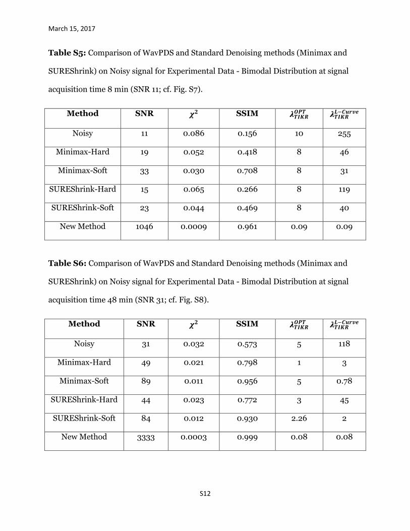
Table S5: Comparison of WavPDS and Standard Denoising methods (Minimax and
SUREShrink) on Noisy signal for Experimental Data - Bimodal Distribution at signal
acquisition time 8 min (SNR 11; cf. Fig. S7).
Method SNR 𝝌𝟐 SSIM 𝝀𝑻𝑰𝑲𝑹𝑶𝑷𝑻 𝝀𝑻𝑰𝑲𝑹
𝑳−𝑪𝒖𝒓𝒗𝒆
Noisy 11 0.086 0.156 10 255
Minimax-Hard 19 0.052 0.418 8 46
Minimax-Soft 33 0.030 0.708 8 31
SUREShrink-Hard 15 0.065 0.266 8 119
SUREShrink-Soft 23 0.044 0.469 8 40
New Method 1046 0.0009 0.961 0.09 0.09
Table S6: Comparison of WavPDS and Standard Denoising methods (Minimax and
SUREShrink) on Noisy signal for Experimental Data - Bimodal Distribution at signal
acquisition time 48 min (SNR 31; cf. Fig. S8).
Method SNR 𝝌𝟐 SSIM 𝝀𝑻𝑰𝑲𝑹𝑶𝑷𝑻 𝝀𝑻𝑰𝑲𝑹
𝑳−𝑪𝒖𝒓𝒗𝒆
Noisy 31 0.032 0.573 5 118
Minimax-Hard 49 0.021 0.798 1 3
Minimax-Soft 89 0.011 0.956 5 0.78
SUREShrink-Hard 44 0.023 0.772 3 45
SUREShrink-Soft 84 0.012 0.930 2.26 2
New Method 3333 0.0003 0.999 0.08 0.08

March 15, 2017
S13
Figure S3: Model Data - Bimodal Distribution (cf. Fig. 5) with SNR = 3: Results of new
WavPDS method compared to standard wavelet denoising methods such as Minimax
and SUREShrink using hard and soft noise thresholding. Blue – Model Signal
(Reference), Red – Noisy Signal, Black – Denoised Signal. A) Comparison of Noisy
and Denoised signals; B) Comparison of Model signals and Denoised signals; C)
Distance Distributions from Noisy, Denoised, and Model signals.

March 15, 2017
S14
Figure S4: Model Data - Bimodal Distribution (cf. Fig. 5) with SNR = 10: Results of
new WavPDS method compared to standard wavelet denoising methods such as
Minimax and SUREShrink using hard and soft noise thresholding. Blue – Model Signal
(Reference), Red – Noisy Signal, Black – Denoised Signal. A) Comparison of Noisy
and Denoised signals; B) Comparison of Model signals and Denoised signals; C)
Distance Distributions from Noisy, Denoised, and Model signals.

March 15, 2017
S15
Figure S5: Experimental Data - Unimodal Distribution (cf. Fig. 7) with 14 min of
acquisition time (SNR = 3.8): Results of WavPDS method compared to standard
wavelet denoising methods such as Minimax and SUREShrink using hard and soft noise
thresholding. Blue – Model Signal (Reference), Red – Noisy Signal, Black – Denoised
Signal. A) Comparison of Noisy and Denoised signals; B) Comparison of Reference
signals and Denoised signals; C) Distance Distributions from Noisy, Denoised, and
Reference signals. Denoised signal at 952 min was used as the Reference.

March 15, 2017
S16
Figure S6: Experimental Data - Unimodal Distribution (cf. Fig. 7) with 112 min of
acquisition time (SNR = 6.8): Results of new WavPDS method compared to standard
wavelet denoising methods such as Minimax and SUREShrink using hard and soft noise
thresholding. Blue – Reference Signal, Red – Noisy Signal, Black – Denoised Signal.
A) Comparison of Noisy and Denoised signals; B) Comparison of Reference signals and
Denoised signals; C) Distance Distributions from Noisy, Denoised, and Reference
signals. Denoised signal at 952 min was used as the Reference.

March 15, 2017
S17
Figure S7: Experimental Data - Bimodal Distribution (cf. Fig. 8) with 8 min of
acquisition time (SNR = 11): Results of new WavPDS method compared to standard
wavelet denoising methods such as Minimax and SUREShrink using hard and soft noise
thresholding. Blue – Reference Signal, Red – Noisy Signal, Black – Denoised Signal.
A) Comparison of Noisy and Denoised signals; B) Comparison of Reference signals and
Denoised signals; C) Distance Distributions from Noisy, Denoised, and Reference
signals. Denoised signal at 360 min was used as the Reference.
March 15, 2017
S18
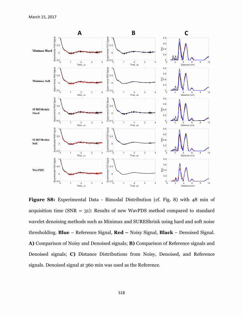
Figure S8: Experimental Data - Bimodal Distribution (cf. Fig. 8) with 48 min of
acquisition time (SNR = 31): Results of new WavPDS method compared to standard
wavelet denoising methods such as Minimax and SUREShrink using hard and soft noise
thresholding. Blue – Reference Signal, Red – Noisy Signal, Black – Denoised Signal.
A) Comparison of Noisy and Denoised signals; B) Comparison of Reference signals and
Denoised signals; C) Distance Distributions from Noisy, Denoised, and Reference
signals. Denoised signal at 360 min was used as the Reference.

March 15, 2017
S19
S8. EXAMPLE OF SIGNAL DENOISING BEFORE BASELINE SUBTRACTION
Figure S9: Comparison of Noisy signal (after 18 hr of signal averaging) and WavPDS
Denoised signal before baseline subtraction. Baseline is determined by fitting the last
several points of the denoised spectrum by a straight line. The 𝑙𝑜𝑔 of the pulsed dipolar
signal (log(𝑆(𝑡))) is plotted versus the evolution time (𝜇s) for a sub-µM concentration of
spin labeled IgE cross-linked with trivalent DNA-DNP ligand in PBS buffer solution.7
(After baseline removal the SNR is 3.8.) This figure was provided by Siddarth
Chandrasekaran (ACERT).

March 15, 2017
S20
S9. USE OF L-CURVE TO DETERMINE 𝝀
Figure S10: L-curve plots to determine 𝜆 for Noisy signals at SNRs 30, 10, and 3, and
L-curve plots of their respective WavPDS Denoised signals for Model Data - Bimodal
Distribution (as shown in Fig. 5). Red – Noisy Signal L-curve plots, Black – Denoised
L-curve plots.

March 15, 2017
S21
Figure S11: L-curve plot to determine 𝜆 for Noisy signal at signal acquisition times 952,
112, and 14 min, and the L-curve plot of their respective WavPDS Denoised signals for
Experimental Data - Unimodal Distribution (cf. Fig. 7). Red –Noisy Signal L-curve
plots, Black – Denoised L-curve plots.

March 15, 2017
S22
S10. COMPARISON OF A LOW-PASS FILTER WITH WavPDS
Fig. S12: Experimental Data—Bimodal Distribution (cf. Fig. 8) with 48 min of
acquisition time (SNR = 31): Results of WavPDS method compared to low-pass filtering.
Blue—Reference signal; Red—Noisy signal; Black—Denoised signal. A) Comparison of
the Noisy and Denoised Signals; B) Comparison of Reference and Denoised signals.
Denoised signal at 360 min was used as the Reference.

March 15, 2017
S23
S11. EXAMPLE OF SPIN ECHO DENOISING
A
B
Figure S13: Echo Signal Denoising: Red - Original Noisy Signal, Black - Denoised
Signal: A) Dispersion where SNR goes from 4 to 1.7 × 10⁷ by denoising; B) Absorption
where SNR of 19 becomes 9.0 × 10⁶. The sample was a 20 𝜇M solution of biradical
𝑝𝑖𝑝𝑒𝑟𝑖𝑑𝑖𝑛𝑦𝑙 − 𝐶𝑂2 − (𝑝ℎ𝑒𝑛𝑦𝑙)4 − 𝑂2𝐶 − 𝑝𝑖𝑝𝑒𝑟𝑖𝑑𝑖𝑛𝑦𝑙 6 and the 𝜋 2⁄ and 𝜋 2⁄ pulses were 2
ns providing full coverage. Coiflet 3 wavelet was used. This figure was provided by Dr.
Peter Borbat (ACERT).