Support Vector Classi cation with Positive … with Positive Homogeneous Risk Functionals In addition, the principle of the structural risk minimization does not mention how it treats

Journal of Machine Learning Research 1 (2013) 1-* Submitted **; Published **

RESEARCH REPORT # 2013-4

Risk Management and Financial Engineering LabDepartment of Industrial and Systems Engineering

University of Florida, Gainesville, FL 32611

Support Vector Classificationwith Positive Homogeneous Risk Functionals

Peter Tsyurmasto [email protected]

Stan Uryasev [email protected]

Jun-ya Gotoh [email protected]

JAPAN

Editor: Leslie Pack Kaelbling

Abstract

Support Vector Machine (SVM) is often formulated as a structural risk minimization,which minimizes simultaneously an empirical risk and a regularization. At the same time,SVM can also be interpreted as a maximization of geometric margin. This paper revisitsthese two views on SVM by applying a risk management approach. A generalization ofthe maximum margin formulation is given, and shown to contain several classical versionsof SVMs such as hard margin SVM, ν-SVM, and extended ν-SVM as its special cases,corresponding to the particular choices of risk functional. Under the assumption that theempirical risk function is positive homogeneous, we derived conditions under which thegeneralized formulation is equivalent to several structural risk minimization formulations.Sufficient conditions for the existence of an optimal solution and unbounded solution tothe associated optimization problems are also given. Within the presented framework, wepropose a new classification method based on the difference of two Conditional Value-at-Risk (CVaR) measures, which is robust to outliers. Computational experiments confirmthat this formulation has a superior out-of-sample performance on datasets contaminatedby outliers, compared to ν-SVM.

1. Introduction

Motivation. The success of support vector machine (SVM) is based on a wide range ofconcepts from statistics, functional analysis, computer science, mathematical optimization,etc. This paper is focused on analysis of optimization formulations of SVM.

As presented in textbooks or tutorial papers (e.g., Burges (2000)), the most fundamentalSVM can be traced back to the so-called maximum margin criterion for binary classification.It maximizes the so-called geometric margin when the given sample data set is (linearly)

c©2013 Peter Tsyurmasto, Stan Uryasev and Jun-ya Gotoh .

Tsyurmasto, Uryasev and Gotoh

separable. Suppose we have a training dataset (ξ1, y1), . . . , (ξl, yl) of features ξi ∈ Rmwith binary class labels yi ∈ −1,+1 for i = 1, . . . , l, and a hyperplane specified by theequation wTx+ b = 0, w ∈ Rm \ 0, b ∈ R. The following quantities gauge the degrees ofmisclassification on the basis of the geometric distances from data samples to the hyperplane:

di(w, b) = −yi(wT ξi + b)

‖w‖, for i = 1, . . . , l, (1)

where ‖ · ‖ denotes the Euclidean norm, i.e., ‖ξ‖ :=√ξ2

1 + · · ·+ ξ2m. Inequality di(w, b) ≤ 0

implies that the sample i is correctly classified by the hyperplane, while di(w, b) > 0 implieswrong classification.

With the notation above, the maximum margin criterion is formulated as a minimizationproblem

minimizew,b

maxd1(w, b), ..., dl(w, b). (2)

This criterion is appealing since 1) it is intuitively understandable; 2) it is a straightforwardminimization of the so-called generalization error bound (e.g., Vapnik, 1999), which lookspersuasive for people with deep statistical background. In addition, as long as the data setis separable, the margin maximization can be reduced to a convex quadratic programmingproblem (QP):

minimizew,b

1

2‖w‖2 subject to − yi(wT ξi + b) ≤ −1, i = 1, ..., l.

On the contrary, when the data set is not separable, the resulting convex QP becomes infea-sible, and the soft margin SVM Cortes and Vapnik (1995) is developed by introducing slackvariables. The soft margin SVM can then be considered as the simultaneous minimizationof an empirical risk (associated with the slack variables introduced) and a regularizationterm (usually defined with the Euclidean norm of the normal vector of the hyperplane).

For example, with the aforementioned notation, the C-SVM, the most popular softmargin formulation, is represented by the bi-objective minimization:

minimizew,b

12‖w‖

2 + C · 1l

∑li=1 max1− yi(wT ξi + b), 0, (3)

with some constant C > 0. Note that the constant C is a parameter balancing the twoobjectives and it needs to be determined. Based on this formulation, the C-SVM can beviewed as the structural risk minimization of the following form:

minimize (regularization) + C · (empirical risk). (4)

However, readers may question the logic sketched above: “Why margin maximization(2) is not applied for the inseparable case?” or “ What is the relation between the marginmaximization (2) and C-SVM (3)?”

It is not hard to see that the margin maximization (2) results in a nonconvex optimiza-tion unless the data set is separable. But do we have any statistical (not tractability-based)motivation for avoiding the nonconvexity?

2

SVC with Positive Homogeneous Risk Functionals

In addition, the principle of the structural risk minimization does not mention how ittreats the trade-off between the empirical risk and the regularization. In other words, itcan also be formulated in either

minimize (empirical risk) subject to (regularization) ≤ E with a constant E, (5)

or

minimize (regularization) subject to (empirical risk) ≤ −D with a constant D. (6)

However, with the empirical risk function employed in C-SVM (3), each of the aboveformulations (4), (5) and (6) results in a different classifier. In fact, C-SVM of the form(5) with E > 0 results in a meaningless solution with w = 0, in which no hyperplane isobtained. On the other hand, it is proved that the ν-SVM (Scholkopf et al., 2000), anotherpopular soft margin SVM, does not depend on the difference among the formulations (4),(5) and (6).

Approach: A Generalized Risk Minimization. The main focus of this paper is tofind what factor makes such a difference. To explore this, we apply a risk managementapproach to the classification problem. The idea of the approach is to view the originalcriterion (2) as a minimization problem with objective function R(d1, . . . , dl) referred to asrisk functional and defined on geometric margins d1, . . . , dl:

minimizew,b

R(d1(w, b), . . . , dl(w, b)), (7)

where R : Rl → R and di is defined in (1). In other words, optimization problem (2) is aspecial case of (7) when risk functional R(d1, . . . , dl) = maxd1, ..., dl is applied.

The area of risk management has been extensively grown in recent years. Specifically,value-at-risk (VaR) and conditional value-at-risk (CVaR) (Rockafellar and Uryasev, 2000)are currently widely used to monitor and control the market risk of financial instruments(Jorion, 1997; Duffie and Pan, 1997). A comprehensive recent study of risk measures canbe found in Rockafellar and Uryasev (2013).

A merit of the generalized representation of the form (7) is to provide a unified schemefor various existing SVM formulations. Specifically, we show that hard-margin SVM (Boseret al., 1992), ν-SVM (Scholkopf et al., 2000), extended ν-SVM (Perez-Cruz et al., 2003)and VaR-SVM (Tsyurmasto et al., 2013) in primal can be represented in compact formswith risk functionals (max-functional, conditional value-at-risk, value-at-risk) and derivedfrom formulation (7).

It is not surprising that the form (7) has a profound relation to the structural riskminimization forms (4), (5) and (6), but the relation among them has been explored onlyin a limited number of articles by specifying its own structure. For example, Perez-Cruzet al. (2003); Gotoh and Takeda (2005) study the relation of the ν-SVM (Scholkopf et al.,2000) to the optimization problem of the form (7) with the CVaR. Recently, Gotoh et al.(2013a) develop a class of generalized formulations of SVM on the basis of the so-calledcoherent risk measures (Artzner et al., 1999), which includes the max-functional and theCVaR as special cases. The novelty of this paper is in more general assumptions on riskfunctional. In particular, our analysis can be applied to nonconvex risk measures, which

3


are not covered by the existing papers. Further we show that the considered approach canderive a more general set of classifiers.

Specifically, we consider a class of risk functionals that are positive homogeneous. Wefirst show that with this assumption, the structural risk minimizations of the differentforms (4), (5) and (6), have the same set of optimal classifiers if the optimal value of (7) isnonpositive; On the other hand, neither (4), (5) or (6) provides any classifier if the optimalvalue of (7) is positive (Figure 2). The paper derives a sufficient condition for the exsitenceof optimal solutions of the considered formulations. It is noteworthy that the obtainedcondition can be checked before the optimization, and is consistent with the fact pointedout by Burges (2000); Chang and Lin (2002); Gotoh and Takeda (2005); Gotoh et al. (2013b)where ν-SVM is shown to be applicable not for all values of parameter ν in the range [0, 1].

In addition, if the risk measure is positive homogeneous, the set of optimal classifiersobtained by either of the structural risk minimizations (4), (5) or (6) does not depend onthe parameters C,D or E. Namely, without bothering how to set those values, we can setC = D = E = 1 (Figure 2). This fact is pointed out in Scholkopf et al. (2000) for theν-SVM by using the duality. In contrast, we show without duality that such a propertycomes from the positive homogeneity of the corresponding risk functional. On the otherhand, the aforementioned dependence on the parameters in the C-SVM can be explainedby lack of positive-homogeneity.

A New Formulation. As a practical application of the developed methodology, we pro-pose a new classification method referred to as CVaR-(αL, αU )-SVM with lower and upperparameters, αL and αU such that 0 ≤ αL < αU < 1. CVaR-(αL, αU )-SVM is a specialcase of the form (7) so that functional R is roughly an average between 100αL and 100αUpercentiles of the set d1(w, b), . . . , dl(w, b) for each pair w, b. In fact, ν-SVM is a specialcase of CVaR-(αL, αU )-SVM with parameters αL = 1− ν and αU = 1. The proposed clas-sifier has an additional parameter αU , which specifies that (1 − αU ) · 100% data sampleswith highest distances to the hyperplane are disregarded. When dataset does not containoutliers, the parameter αU can be chosen (almost) equal to 1 and, thus, CVaR-(αL, αU )-SVM performs as good as ν-SVM. However, when dataset is contaminated by outliers,CVaR-(αL, αU )-SVM has an advantage of stability to outliers, compared to ν-SVM. Theformulation of CVaR-(αL, αU )-SVM can be related to an existing formulation known as theramp loss SVM Collobert et al. (2006). An advantage of the proposed formulation is parallelto that of ν-SVM over the C-SVM. Namely, the CVaR-(αL, αU )-SVM has two interpretableparameters αL, αU , while the ramp loss SVM has a difficulty in the interpretation of theincluded parameter, and some exhaustive search is required for the parameter tuning. Thecomputational experiments confirm that in presence of outliers, CVaR-(αL, αU )-SVM hasa superior out-of-sample performance versus ν-SVM.

The contribution of this paper can be summarized as follows:

• Based on the geometric margin, which is employed in the maximum margin SVM, weprovide a unified scheme which contains several well-known SVMs;

• With the notion of risk functionals, we establish relations between existing SVMclassifiers, and reveal that positive homogeneity plays a central role in the equivalenceamong the different formulations;

4


• We establish a sufficient condition for existence of optimal solution of (7).;

• We develop a nonlinear extension of (7);

• As a special case of (7), we propose a new classifier stable to outliers and empiricallyconfirm its robust properties.

The paper is structured as follows. Section 2 presents a risk management approach to clas-sification problem by following a brief overview of the existing formulations and shows thatSVMs can be expressed in compact form in terms of risk functionals. Section 3 proposesa classification model based on positive homogeneous risk functionals. Section 4 proposesCVaR-(αL, αU )-SVM. Section 5 extends to nonlinear CVaR-(αL, αU )-SVM. Section 6 con-tains results of computational experiments. Section 7 concludes.

2. Representation of SVMs with Risk Functionals in Primal

A Brief Overview of Existing SVM Formulations for Binary Classification. Let(ξ1, y1), . . . , (ξl, yl) be a training dataset of features ξi ∈ Rm with binary class labels yi ∈−1,+1 for i = 1, . . . , l. The original features ξ1, . . . , ξl ∈ Rm are transformed into featuresφ(ξ1), . . . , φ(ξl) ∈ Rn, respectively, with the mapping φ : Rm → Rn. The goal of the SVMis then to construct a hyperplane specified by the equation wTx + b = 0, w ∈ Rn, b ∈ R,which separates the transformed features φ(ξ1), . . . , φ(ξl) with class labels +1 and −1 fromeach other in Rn space.

In order to find a hyperplane on the basis of the given training set and an (implicit)mapping φ, minimizing violation of separation is a bottom line. We say that the dataset isseparable if there exists (w, b) ∈ Rn\0×R such that for each i = 1, ..., l, yi(w

Tφ(ξi)+b) > 0.On the other hand, a data point ξi is considered to be wrongly classified if yi(w

Tφ(ξi)+b) < 0for a given (w, b). A reasonable criterion for determining a (w, b) is to place the hyperplaneso that the geometric distance from the worst classified data sample would be the nearest ifdataset is inseparable, or that from the nearest data is maximized if data set is separable.This rule is formulated as a fractional programming (FP) problem:

maximizew,b

mini

yi(w

Tφ(ξi) + b)

‖w‖: i = 1, ..., l

. (8)

In this paper, the quantity yi(wTφ(ξi)+b) is referred to as the margin (of a sample i), while

yi(wTφ(ξi)+b)/‖w‖ is referred to as the geometric margin (of a sample i). The optimization

problem (8) is known to be rewritten by a quadratic programming (QP) problem:

maximizew,b

12‖w‖

2

subject to yi(wTφ(ξi) + b) ≥ 1, i = 1, ..., l,

(9)

if the dataset is separable under the mapping φ. This approach is known as hard marginSVM (see, e.g., Boser et al. (1992)). It is, however, noteworthy that the FP (8) remainswell-defined even when dataset is inseparable, whereas QP (9) is then infeasible, i.e., it hasno feasible solution.

5


In order to deal with non-separable data sets, formulation (9) was extended by intro-ducing slack variables z1, ..., zl:

minimizew,b,z

12‖w‖

2 + Cl

∑li=1 zi

subject to yi(wTφ(ξi) + b) ≥ 1− zi, i = 1, ..., l,

zi ≥ 0, i = 1, ..., l,

(10)

where C > 0 is a parameter to be tuned. (10) is referred to as C-SVM. It should be notedthat (10) is rewritten by an unconstrained (convex) minimization of the form:

minimizew,b

1

2‖w‖2 +

C

l

l∑i=1

[1− yi(wTφ(ξi) + b)]+, (11)

where [x]+ := maxx, 0. The form (11) is referred to as a class of structural risk min-imization, which is often considered as a central principle for machine learning methods.Namely, (11) is considered as the simultaneous minimization of the empirical classificationerror term

∑li=1[1− yi(wTφ(ξi) + b)]+ and the regularization term ‖w‖, which is added to

control overfitting.On the other hand, the interpretation of the empirical error term has been left ambiguous

in the sense that a data sample contributes to this term if the margin is less than 1 andno clear interpretation is given for the meaning of the value of 1. At the same time, theinterpretation of the parameter C is also not clear.

As a remedy for the ambiguous interpretation of the involved constants, i.e., 1 and C,Scholkopf et al. (2000) develop an alternative known as ν-SVM:

minimizew,b,ρ,z

12‖w‖

2 − νρ+ 1l

∑li=1 zi

subject to yi(wTφ(ξi) + b) ≥ ρ− zi, i = 1, ..., l,

zi ≥ 0, i = 1, ..., l,

(12)

where ν ∈ (0, 1] is a parameter to be tuned.Corresponding to (12), Perez-Cruz et al. (2003) pose an extended formulation:

minimizew,b,ρ,z

−νρ+ 1l

∑li=1 zi

subject to yi(wTφ(ξi) + b) ≥ ρ− zi, i = 1, ..., l,

zi ≥ 0, i = 1, ..., l,‖w‖ = 1,

(13)

where ν ∈ (0, 1] is a parameter to be tuned. Eν-SVM (13) is a nonconvex minimizationformulation, but it extends the lower bound νmin of admissible range of ν-SVM to (0, νmax].

We have so far overviewed several popular SVM formulations, and it is not hard to seethat all are based on the margin, yi(w

Tφ(ξi)+b), or geometric margin, yi(wTφ(ξi)+b)/‖w‖,

and eventually formulated as a structural risk minimization form (e.g., (9) (11), (12) and(13)) or an FP (e.g., (8)). It is not hard to see that all these have a common feature informulating a certain trade-off between the empirical risk and the regularization, but it isnot clear how they are related to each other, especially in terms of the parameters therein,such as C in (10) or ν in (12) and (13). One of the purposes of this paper is to revealthe connection among those formulations and to show that the positive homogeneity of therelated function plays an important role.

6


SVM Formulations with Various Risk Functionals. This paper considers the fol-lowing probabilistic setting. Let Ω = ω1, . . . , ωl be a finite sample space of outcomeswith equal probabilities Pr(ωi) = 1

l for i = 1, . . . , l and ξ : Ω → Rn, y : Ω → −1,+1 bea pair of discretely distributed random variables defined as ξ(ωi) = φ(ξi), y(ωi) = yi fori = 1, . . . , l. Random loss function is defined for each outcome ω ∈ Ω and decision variablesw ∈ Rn, b ∈ R by

Lω(w, b) = −y(ω) · [wT ξ(ω) + b]. (14)

Loss function (14) represents a random error on the training set. Namely, negative lossLωi(w, b) < 0 indicates that data sample i is classified correctly, while positive loss Lωi(w, b) >0 indicates that φ(ξi) is classified incorrectly, i = 1, . . . , l.

A random distance function is defined for each outcome ω ∈ Ω and decision variablesw ∈ Rn, b ∈ R as a normalized loss function:

dω(w, b) =Lω(w, b)

‖w‖. (15)

For each outcome ω ∈ Ω, the absolute value of (15) is a Euclidian distance between a vectorξ(ω) and a hyperplane H = x ∈ Rn|wTx + b = 0. Distance function (15) has a discretedistribution of realizations

−yi · [wTφ(ξi) + b]

‖w‖

∣∣∣∣li=1

. (16)

with equal probabilities 1l . Figure 1 shows a histogram for the realizations (16) of distances

of data samples (φ(ξ1), y1), . . . , (φ(ξl), yl) to the hyperplane for some fixed parameters (w, b)of the hyperplane. Samples falling into light area (blue in color) are classified correctly, whilesamples falling into a dark area (red in color) are classified incorrectly. The goal is to selectsuch parameters of hyperplane (w, b) in (15) as to reduce the size of the right tail (markedwith red color) of the histogram.

This problem can be formalized by introducing a risk functional R(·), which converts arandom distance dω(w, b) into a deterministic function R(dω(w, b)):

minimizew,b

R(Lω(w, b)

‖w‖

). (17)

An objective in (17) represents an aggregated loss in the right tail of (15) so that the lowerthe objective in (17), the lower the size of the right tail of (15) exceeding zero. Optimizationproblem (17) can be viewed as a margin-based classifier since it takes into account distancesof data samples to the hyperplane and aggregates them by means of risk functional R(·).Further we assume that R(C) = C for each constant C ∈ R. Each choice of risk functionalR(·) defines a particular classifier.

In the literature of machine learning, the risk functional is usually minimized togetherwith some regularization.

minimizew,b

R (Lω(w, b))

‖w‖, (18)

minimizew,b

R(Lω(w, b)) subject to ‖w‖ = E, E > 0, (19)

7


Figure 1: Histogram of the distances (1) of the data samples (φ(ξ1), y1), . . . , (φ(ξl), yl) to thehyperplane for German Credit Data (The dataset was taken from UCI MachineLearning Repository http://archive.ics.uci.edu/ml/datasets.html) whenthe decision variables are fixed.

minimizew,b

R(Lω(w, b)) subject to ‖w‖ ≤ E, E > 0, (20)

minimizew,b

1

2‖w‖2 subject to R(Lω(w, b)) ≤ −D, D > 0, (21)

minimizew,b

1

2‖w‖2 + C · R(Lω(w, b)), C > 0, (22)

corresponding to particular risk functionals R(·).

Example: Maximum Margin SVM and Hard-Margin SVM. The maximum mar-gin formulation (8) and the hard margin SVM (9) can be related to the worst-case loss (ormaximum loss):

sup(Lω) := maxLω1 , ...,Lωl. (23)

With worst-case loss (23), formulations (8) and (9) are special cases of (17) and (21) (withD = 1), respectively.

Example: C-SVM. Based on (11), the C-SVM (10) corresponds to the above-target-loss:

ATLt(Lω) :=1

l

l∑i=1

[Lωi +t]+. (24)

with t = 1. Indeed, substitution of (24) with (14) into (22) results in (11), or equivalently,(10).

8

http://archive.ics.uci.edu/ml/datasets.html


Example: ν-SVM (Scholkopf et al. (2000)). Using the fact that constraint ρ ≥ 0 isredundant in the formulation as was shown by Burges (2000), ν-SVM (12) can be expressedwith the Conditional Value-at-Risk (CVaR) functional, i.e., R(·) = CVaRα(·), which isgiven by

CVaRα (Lω) := minc

c+

1

(1− α)l

l∑i=1

[Lωi −c]+

, (25)

where α ∈ [0, 1), [x]+ := maxx, 0. By using the (strong) duality theorem of linearprogramming (see, e.g., Boyd and Vandenberghe (2004)), we can obtain a useful formulacomputing the CVaR of a loss Lω. Let L[i] denote the i-th largest element among Lω1 , ...,Lωl

,i.e., L[1] ≥ L[2] ≥ · · · L[l]. Then the CVaR of L is calculated by the formula:

CVaRα(Lω) =1

pl

bpc∑i=1

L[i] + (p− bpc)L[bpc+1]

, (26)

where p = (1− α)l. Consider the case where (1− α)l is an integer k ∈ 1, 2, ..., l, then theformula (26) can be simplified as follows:

CVaRα(L) =1

k

k∑i=1

L[i].

In this sense, the CVaR can be considered as the conditional expectation of L of the largest(1 − α)l elements. (See, e.g., Rockafellar and Uryasev (2013) for the detailed explanationand properties for CVaR).

The relation between ν-SVM and the CVaR minimization was first noticed in Gotohand Takeda (2005).

Example: Extended ν-SVM (Eν-SVM) (Perez-Cruz et al. (2003)). Eν-SVM (13)can be expressed with the CVaR functional (25)

minimizew,b

CVaR1−ν (Lω(w, b)) subject to ‖w‖ = 1, (27)

as was shown by Takeda and Sugiyama (2008). Indeed, substitution of the CVaR with (14)and α = 1− ν into (19) with E = 1 results in (27).

Example: VaR-SVM (Tsyurmasto et al. (2013)). (VaR) is a quantile of the loss,i.e.,

VaRα (Lω) := mincc : PrLω ≤ c ≥ α , (28)

where α ∈ (0, 1). VaR-SVM can be expressed in the form (21) with VaR functional (28):

minimizew,b

1

2‖w‖2 subject to VaRα(Lω(w, b)) ≤ −1. (29)

In contrast to the aforementioned examples, VaRα(Lω(w, b)) is nonconvex with respect tow and b, and accordingly, (29) is a nonconvex minimization, which may have (nonglobal)local minima.

9


3. Relation between SVM Formulations with Risk Functionals

In this section, we establish relations between optimization problems (17)-(22), summarizedin Figure 2. First of all, we find out which of the aforementioned problems have the sameset of classifiers for each risk functional R(·).

Proposition 1 Classifiers defined in primal by optimization problems (17) and (19) pro-vide the same separating hyperplane for each risk functional R(·) and the constant E > 0.

Indeed, if (w∗, b∗) is an optimal solution of (17), then ( Ew∗

‖w∗‖ ,Eb∗

‖w∗‖) is an optimal solution of

(19). Conversely, if (w∗∗, b∗∗) is an optimal solution of (19), then λ(w∗∗, b∗∗) is an optimalsolution of (17) for each λ > 0.

Notice that the constant E in (19) and 20 can be set E = 1 due to the positive homogene-ity of the norm function. Thus the optimization problems (19) and 20 can be equivalentlyrecast with E = 1:

minimizew,b

R(Lω(w, b)) subject to ‖w‖ = 1, (30)

minimizew,b

R(Lω(w, b)) subject to ‖w‖ ≤ 1. (31)

Next we focus on a special case of positive homogeneous risk functionals, for whichnorm-constrained, risk-constrained and unconstrained formulations (20)-(22) under someadditional conditions define the same classifiers.

3.1 Positive Homogeneous Risk Functionals

Definition 2 (Positive Homogeneity) R(λX) = λR(X) for each random variable X andconstant λ > 0, λ ∈ R.

Note that among the risk functionals listed in the previous section, ATLt, which is givenin (24), does not satisfy this property, and accordingly, we exclude the C-SVC from theanalysis below. Several examples of positive homogeneous risk functionals are providedbelow.

• sup(Lω) = maxLω1 , . . . ,Lωl Worst-Case Loss

• E(Lω) = 1l

∑li=1 Lωi Expected Loss

• ATL0(Lω) = 1l

∑li=1[Lωi ]+ Above-Zero Loss

• MASDt(Lω) = E(Lω) + tE([Lω −E(Lω)]+) with t ≥ 0 Mean-AbsoluteSemi-Deviation

• VaR(Lω) = minc c : PrLω ≤ c ≥ α Value-at-Risk

• CVaR(Lω) = minc

c+ 1

(1−α)l

∑li=1 [Lωi −c]+

Conditional Value-at-Risk

• CRM(Lω) = maxq1,...,ql

l∑

i=1qi Lωi : (q1, ..., ql) ∈ Q with Q ⊂ (q1, ..., ql) :

l∑i=1

qi = 1, qi ≥

0, i = 1, ..., l Coherent Risk Measures

10


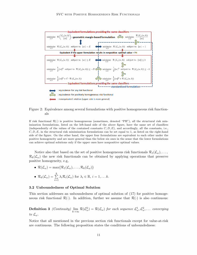
Figure 2: Equivalence among several formulations with positive homogeneous risk function-als

If risk functional R(·) is positive homogeneous (sometimes, denoted “PH”), all the structural risk min-imization formulations, listed on the left-hand side of the above figure, have the same set of classifiers(independently of the values of the contained constants C,D,E), and accordingly, all the constants, i.e.,C,D,E, in the structural risk minimization formulations can be set equal to 1, as listed on the right-handside of the figure. On the other hand, the upper four formulations are equivalent to each other under thepositive homogeneity and are more general than the below six ones in the sense that the lower formulationscan achieve optimal solutions only if the upper ones have nonpositive optimal values.

Notice also that based on the set of positive homogeneous risk functionals R1(Lω), . . . ,Rk(Lω) the new risk functionals can be obtained by applying operations that preservepositive homogeneity, e.g,

• R(Lω) = maxR1(Lω), . . . ,Rk(Lω)

• Rk(Lω) =k∑i=1

λiRi(Lω) for λi ∈ R, i = 1, . . . k.

3.2 Unboundedness of Optimal Solution

This section addresses an unboundedness of optimal solution of (17) for positive homoge-neous risk functional R(·). In addition, further we assume that R(·) is also continuous:

Definition 3 (Continuity) limk→∞

R(Lkω) = R(Lω) for each sequence L1ω,L2

ω, . . . converging

to Lω.

Notice that all mentioned in the previous section risk functionals except for value-at-riskare continuous. The following proposition states the conditions of unboundedness:

11


Proposition 4 Suppose that R(·) is a positive homogeneous and continuous risk functional.Then optimization problem (17) is unbounded if

minR(−y(ω),R(y(ω))) < 0. (32)

The proof of Proposition 4 is sketched in Appendix A.

3.3 Equivalence of Formulations with Positive Homogeneous Risk Functionals

Support Vector Machine is usually formulated using the structural risk minimization prin-ciple that can be expressed as a tradeoff between empirical risk and the regularization.Classification methods defined in primal as (20)-(22) provide several ways how this tradeoffcan be expressed. With empirical function employed in C-SVM (3), all three formulationsresult in different classifiers. On the other hand, it is proved that all three formulation(20)-(22) with risk functionals CVaR1−ν(·) define ν-SVM (12). This fact can be explainedby positive homogeneity of CVaR risk measure. This section aims at showing that for posi-tive homogeneous risk functionals under a certain condition classifiers specified in primal by(20)-(22) provide the same separating hyperplane, which is also optimal for the geometricmargin formulation (17).

Proposition 5 Suppose that R(·) is a positive homogeneous and continuous risk functional.Then

1. If (w∗, b∗) is an optimal solution of (17) with negative optimal objective value, thenE‖w∗‖(w

∗, b∗) is optimal for (20).

2. If (w∗, b∗) is an optimal solution of (20) and w∗ 6= 0, then λ(w∗, b∗) is an optimalsolution of (17).

The proof of Proposition 5 is sketched in Appendix B.


1. If (w∗, b∗) is optimal solution of (17) with negative optimal objective value, then−D

ζ (w∗, b∗) is an optimal solution of (21), where ζ = |R(Lω(w∗, b∗))|.


The proof of Proposition 6 is sketched in Appendix C.


1. If (w∗, b∗) is optimal solution of (17) with negative optimal objective value, thenCr∗

‖w∗‖(w∗, b∗) is an optimal solution of 22, where r∗ = −R(Lω(w∗,b∗))

‖w∗‖ .


12


The proof of Proposition 7 is sketched in Appendix D.

Remark 8 When (22) have non-zero optimal solutions, (22) determines the same hyper-plane for different values of C > 0. Thus, the parameter C can be set to 1.

Propositions 5-7 imply the following corollary, which summarizes the relation betweenformulations (17), (20), (21), 22 .

Corollary 9 Suppose that R(·) is a positive homogeneous and continuous risk functional.Then

1. When (17) has a negative optimal objective value, optimization problems (17), (20),(21), 22 determine the same separating hyperplane.

2. When (17) has a positive or zero optimal objective value, optimization problems (20),(22) have a trivial solution (w = 0) and (21) is infeasible.

4. Existence of Optimal Solution

In this section, we explore under what condition there exists an optimal solution of opti-mization problem (17). We formulate the result for positive homogeneous and lower semi-continuous risk functionals R(·). The lower semi-continuity assumption is more generalthan continuity and hold for all risk functionals listed in this dissertation.

Proposition 10 (Existence of Optimal Solution) Suppose that R(·) is positive homo-geneous and lower semi-continuous. Then (17) has an optimal solution if

minR(−y(ω)),R(y(ω)) > 0 (33)

The proof of Proposition 10 is sketched in Appendix E.We should note that continuity is not necessary for the existence of an optimal solution or

unboundedness of the minimization. In fact, although VaR, defined in (28), does not satisfythe (upper semi-)continuity, its minimization is unbounded if (32) holds (see Theorem 2 ofTsyurmasto et al. (2013) for details).

Example: Expected loss. Consider the case where the expected loss is used as the riskmeasure, i.e.,

R(Lω(w, b)) = E[Lω(w, b)] = −∑ω∈Ω

Pr(ω)y(ω)(wTφ(ξ(ω)) + b).

Note that the expected loss is positive homogeneous and convex on Rm (i.e., continuous).In this case, we have

minω∈ΩR(−y(ω)),R(y(ω)) = min1

l

l∑i=1

yi,−1l

l∑i=1

yi

= min1l (l+ − l−), 1

l (l− − l+) =

< 0 if l+ 6= l−,= 0 if l+ = l−.

13


where l+ := |i : yi = +1| and l− := |i : yi = −1|. Then Proposition 10 indicates thatthe expected loss-based SVM can have an optimal solution only if the number of samplesof yi = +1 is equal to that of yi = −1. This is consistent with the result in Gotoh et al.(2013b), where a general probability setting pi = Pr(ωi) is employed and the authors showthat the condition

∑li=1 piyi = 0 is the necessary and sufficient for the optimality. In

addition, we should note that the expected loss based SVM admits any b as an optimalsolution even when the condition l+ = l− holds, i.e., the number of the samples in eachclass is equal, and accordingly, it has the bounded optimal value.

Example: Worst-case loss (or maximum loss) Given a set of data samples Ω =ω1, ..., ωl (or more specifically, (ξ1, y1), . . . , (ξl, yl)), consider the risk measure R(·) =sup(·). The condition (33) is then given by

minsup−y1, . . . ,−yl, supy1, . . . , yl = min1, 1 = 1 > 0.

Namely, when the worst-case loss is employed, the condition (33) is satisfied if and only ifthere is at least one sample of each class.

Example: CVaR. Consider the case where the CVaR is used as the risk measure. Byusing the formula (26), we can easily check if the condition (33) is satisfied. Indeed, we cansee that R(y(ω)) > 0 holds if and only if (1− α)l < 2l+ holds where l+ := |i : yi = +1|;R(−y(ω)) > 0 holds if and only if (1 − α)l < 2l− holds where l− := |i : yi = −1|.Accordingly, the condition (33) for the CVaR is given by

α >1

l(1− 2 minl+, l−). (34)

It is noteworthy that this bound is consistent with the admissible range of the parame-ter ν for ν-SVM Burges (2000). Also the condition (33) is consistent with the admissi-ble range for the ν-SVM shown in Chang and Lin (2002) and the condition in Lemma2.2 of Gotoh and Takeda (2005), where the condition for the existence of an optimal so-lution of the geometric margin-based CVaR minimization formulation is given by α ≥1 − 2 min

∑i:yi=+1 pi,

∑i:yi=−1 pi with the probability pi := Pr(ωi). On the other hand,

the condition (32) implies that for

α <1

l(1− 2 minl+, l−),

optimization problems (18) and (19)-(22) are unbounded.

Example: VaR. Let us find an admissible range of parameter α for VaR-SVM (29). Sincey(ω) is discretely distributed random variables with realizations −1, . . . ,−1︸︷︷︸

l−

,+1, . . . ,+1︸︷︷︸l+

,

VaRα(±y(ω)) =

≥ 0 if α ≥ l∓+1

l ,

< 0 if α < l∓+1l .

(35)

Thus, condition (33) holds when α ≥ minα+, α− + 1l , while condition (32) holds when

α < minα+, α− + 1l (here we denote α+ = l+

l and α− = l−l fractions of samples with

positive and negative class labels, accordingly).

14


5. CVaR-(αL, αU)-SVM

In this section, we propose a new classifier formulated in the primal as

minw,b

(1− αL) · CVaRαL(dω(w, b))− (1− αU ) · CVaRαU (dω(w, b)) (36)

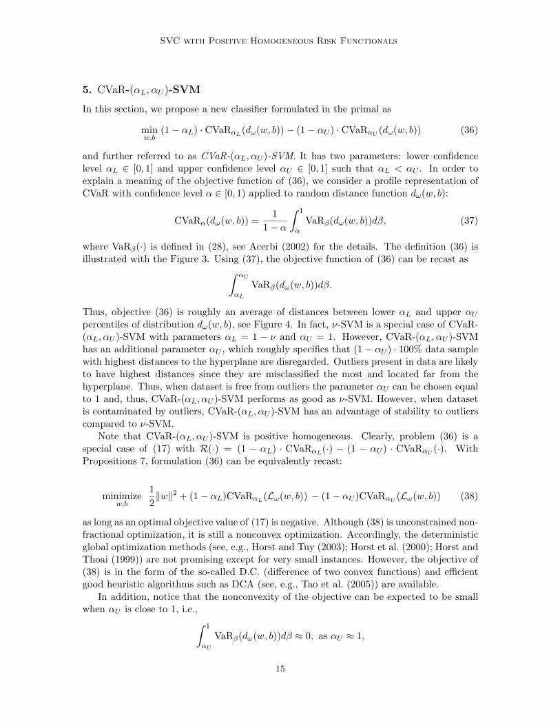
and further referred to as CVaR-(αL, αU )-SVM. It has two parameters: lower confidencelevel αL ∈ [0, 1] and upper confidence level αU ∈ [0, 1] such that αL < αU . In order toexplain a meaning of the objective function of (36), we consider a profile representation ofCVaR with confidence level α ∈ [0, 1) applied to random distance function dω(w, b):

CVaRα(dω(w, b)) =1

1− α

∫ 1

αVaRβ(dω(w, b))dβ, (37)

where VaRβ(·) is defined in (28), see Acerbi (2002) for the details. The definition (36) isillustrated with the Figure 3. Using (37), the objective function of (36) can be recast as∫ αU

αL

VaRβ(dω(w, b))dβ.

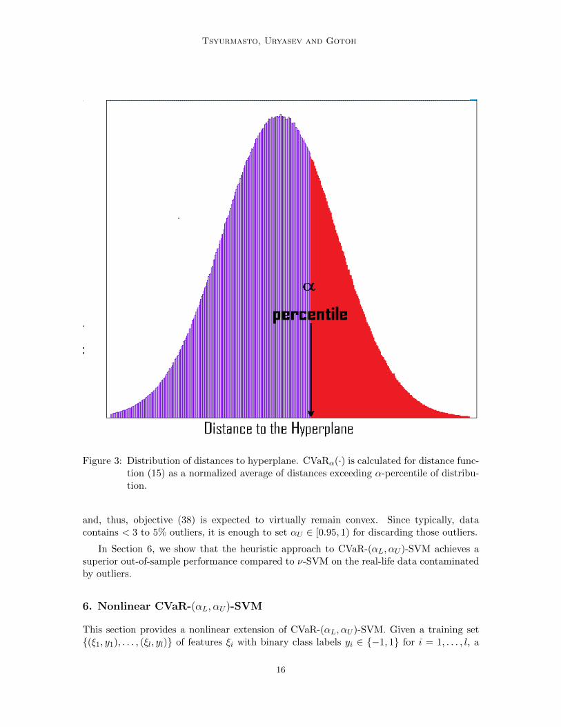
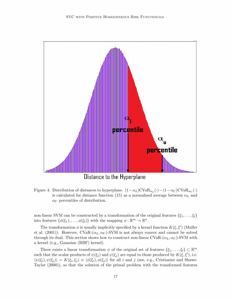
Thus, objective (36) is roughly an average of distances between lower αL and upper αUpercentiles of distribution dω(w, b), see Figure 4. In fact, ν-SVM is a special case of CVaR-(αL, αU )-SVM with parameters αL = 1 − ν and αU = 1. However, CVaR-(αL, αU )-SVMhas an additional parameter αU , which roughly specifies that (1− αU ) · 100% data samplewith highest distances to the hyperplane are disregarded. Outliers present in data are likelyto have highest distances since they are misclassified the most and located far from thehyperplane. Thus, when dataset is free from outliers the parameter αU can be chosen equalto 1 and, thus, CVaR-(αL, αU )-SVM performs as good as ν-SVM. However, when datasetis contaminated by outliers, CVaR-(αL, αU )-SVM has an advantage of stability to outlierscompared to ν-SVM.

Note that CVaR-(αL, αU )-SVM is positive homogeneous. Clearly, problem (36) is aspecial case of (17) with R(·) = (1 − αL) · CVaRαL(·) − (1 − αU ) · CVaRαU (·). WithPropositions 7, formulation (36) can be equivalently recast:

minimizew,b

1

2‖w‖2 + (1− αL)CVaRαL(Lω(w, b)) − (1− αU )CVaRαU (Lω(w, b)) (38)

as long as an optimal objective value of (17) is negative. Although (38) is unconstrained non-fractional optimization, it is still a nonconvex optimization. Accordingly, the deterministicglobal optimization methods (see, e.g., Horst and Tuy (2003); Horst et al. (2000); Horst andThoai (1999)) are not promising except for very small instances. However, the objective of(38) is in the form of the so-called D.C. (difference of two convex functions) and efficientgood heuristic algorithms such as DCA (see, e.g., Tao et al. (2005)) are available.

In addition, notice that the nonconvexity of the objective can be expected to be smallwhen αU is close to 1, i.e.,∫ 1

αU

VaRβ(dω(w, b))dβ ≈ 0, as αU ≈ 1,

15


Figure 3: Distribution of distances to hyperplane. CVaRα(·) is calculated for distance func-tion (15) as a normalized average of distances exceeding α-percentile of distribu-tion.

and, thus, objective (38) is expected to virtually remain convex. Since typically, datacontains < 3 to 5% outliers, it is enough to set αU ∈ [0.95, 1) for discarding those outliers.

In Section 6, we show that the heuristic approach to CVaR-(αL, αU )-SVM achieves asuperior out-of-sample performance compared to ν-SVM on the real-life data contaminatedby outliers.

6. Nonlinear CVaR-(αL, αU)-SVM

This section provides a nonlinear extension of CVaR-(αL, αU )-SVM. Given a training set(ξ1, y1), . . . , (ξl, yl) of features ξi with binary class labels yi ∈ −1, 1 for i = 1, . . . , l, a

16


Figure 4: Distribution of distances to hyperplane. (1−αL)CVaRαL(·)−(1−αU )CVaRαU (·)is calculated for distance function (15) as a normalized average between αL andαU percentiles of distribution.

non-linear SVM can be constructed by a transformation of the original features ξ1, . . . , ξlinto features φ(ξ1), . . . , φ(ξl) with the mapping φ : Rm → Rn.

The transformation φ is usually implicitly specified by a kernel function K(ξ, ξ′) (Mulleret al. (2001)). However, CVaR-(αL, αU )-SVM is not always convex and cannot be solvedthrough its dual. This section shows how to construct non-linear CVaR-(αL, αU )-SVM witha kernel (e.g., Gaussian (RBF) kernel).

There exists a linear transformation ψ of the original set of features ξ1, . . . , ξl ⊂ Rmsuch that the scalar products of ψ(ξj) and ψ(ξj) are equal to those produced by K(ξ, ξ′), i.e.〈ψ(ξi), ψ(ξj)〉 = K(ξi, ξj) ≡ 〈φ(ξi), φ(ξj)〉 for all i and j (see, e.g., Cristianini and Shawe-Taylor (2000)), so that the solution of the primal problem with the transformed features

17


ψ(ξ1), . . . , ψ(ξl) ⊂ Rn coincides with that for the dual problem with the kernel K(ξ, ξ′)corresponding to the original transformation φ (Chapelle (2007)).

For features ξ1, . . . , ξl, the kernel K(ξ, ξ′) yields a positive definite kernel matrix K =K(ξi, ξj)i,j=1,...,l, which can be decomposed as

K = V ΛV T ≡ (V Λ12 )(V Λ

12 )T , (39)

where Λ = diag(λ1, . . . , λl) is a diagonal matrix with eigenvalues λ1 > 0, . . . , λl > 0 andV = (v1, . . . , vl) is an orthogonal matrix with corresponding eigenvectors v1, . . . , vl of K.

The representation (39) implies that ψ : ξi → (V Λ12 )i, i = 1, . . . , l, is the sought linear

transformation, where (V Λ12 )i is row i of the matrix (V Λ

12 ). Thus, the nonlinear version of

(36) has the following explicit formulation

minimizeλ,λ0

1

2‖λ‖2 + (1− αL)CVaRαL(Lω(λ, λ0)) − (1− αU )CVaRαU (Lω(λ, λ0)) (40)

with new decision variables λ ∈ Rl, λ0 ∈ R and discretely distributed loss function Lω(λ, λ0)given by observations (scenarios)

Lωi(λ, λ0) = −yi[λTφ(ξi) + λ0],

and φ(ξi) = (V Λ12 )i for i = 1, . . . , l.

7. Computational Experiment

The computations are performed with MATLAB using Portfolio Safeguard (PSG)1 solver,which applies advanced techniques for optimizing CVaR function. With PSG, solving prob-lems involves three main stages:

1. Mathematical formulation of optimization problem using precoded CVaR functions.Typically, a problem formulation involves 5-10 operators of a meta-code. See, for in-stance, Appendix F with the example of problem formulation for optimization problem(38).

2. Preparation of data for the PSG functions in an appropriate format. In our experi-ment, CVaR functions are defined on the matrix of training samples (ξ1, y1), . . . , (ξl, yl).

3. Solving the optimization problem with PSG using the predefined problem statementand data for PSG functions. The problem can be solved in several PSG environments,such as MATLAB environment and Run-File (Text) environment.

The problems (36) and ν-SVM are solved with datasets from UCI Machine LearningRepository2: Liver Disorders, Heart Disease, Indian Diabetes, German and Ionosphere.

The original features were normalized (zero mean, unit standard deviation). To calculatetesting accuracy, we use 10-fold cross validation. We use 2/3 of the training set to solve(12) and (36) and the remaining 1/3 to fit the parameters ν in (12) and αL, αr in (36).Parameter ν and αL are selected from the grid 0 : 0.05 : 1, while parameter αU is selectedfrom the grid 0.9 : 0.01 : 1.

1. http://www.aorda.com/aod/welcome.action/psg.action

2. http://archive.ics.uci.edu/ml/datasets.html

18

http://www.aorda.com/aod/welcome.action/psg.action

http://archive.ics.uci.edu/ml/datasets.html


Table 1: Experimental results for Liver Disorders Dataset, contaminated by outliers.

ν-SVM accuracy (%) CVaR-(αL, αU )-SVM accuracy (%)Percent of Outliers (%) training testing training testing

Mean Std Mean Std Mean Std Mean Std0 70.43 1.18 66.13 2.09 72.22 1.47 71.17 1.731 69.07 1.81 65.43 2.55 72.72 2.74 71.65 2.655 60.52 2.41 60.65 1.72 72.26 1.35 68.91 1.1410 61.63 1.92 59.57 2.46 74.15 2.01 70.78 1.86

Table 2: Experimental Results for Heart Disease Dataset, contaminated by outliers.


Mean STD Mean STD Mean STD Mean Std0 85.15 1.77 82.09 2.72 85.54 1.13 83.16 1.211 85.15 2.58 82.60 1.44 86.12 1.56 83.27 2.075 84.59 1.54 82.24 2.19 87.17 2.04 83.27 1.6210 75.59 2.36 74.23 3.01 86.64 1.13 83.57 1.74

7.1 Linear SVM

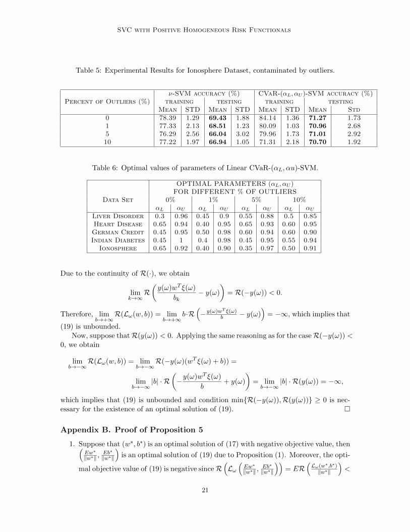
Linear ν-SVM and CVaR-(αL, αU )-SVM performed 66.13% and 71.17% on Liver DisorderDataset, 82.09% and 83.16% on Heart Disease Dataset, 76.05% and 76.29% on IndianDiabetes Dataset, 69.43% and 71.27% on Ionosphere DataSet, accordingly. Outliers weregenerated by artificially multiplying a fraction of 0%, 1%, 5%, 10% of the original datasetby 1000. Tables 1, 2, 4, 3, 5 show performances of ν-SVM and CVaR-(αL, αU )-SVM as thepercentage of outliers increases, the performance of ν-SVM drops, while CVaR-(αL, αU )-SVM has almost the same performance. Tables 7 and 6 show optimal parameters ν forν-SVM and αL, αr for CVaR-(αL, αU )-SVM.

7.2 Non-Linear SVM

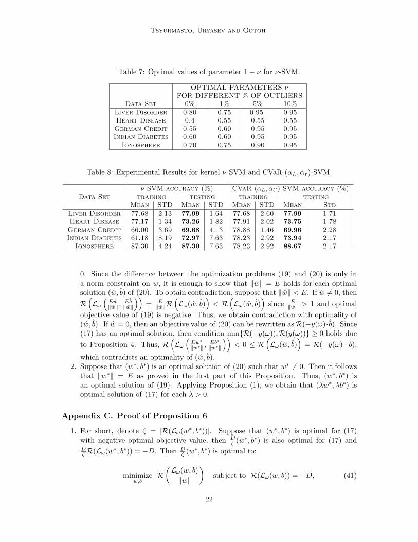
We compare out-of-sample performance of non-linear CVaR-(αL, αU )-SVM against ν-SVMwith Gaussian kernel. The original features are transformed as described in Section 6.Table 8 summarizes results of the experiment. CVaR-(αL, αU )-SVM outperformed ν-SVMon all datasets, especially Indian Diabetes and Ionosphere.

8. Conclusion

The paper presented a unified scheme for classification based on geometric margin. Thescheme encompasses several well-known SVMs. The relation between existing SVMs wasestablished using positive homogeneity of corresponding risk functionals. A unified schemewith linear loss function was extended to non-linear case. As a special case of unified

19


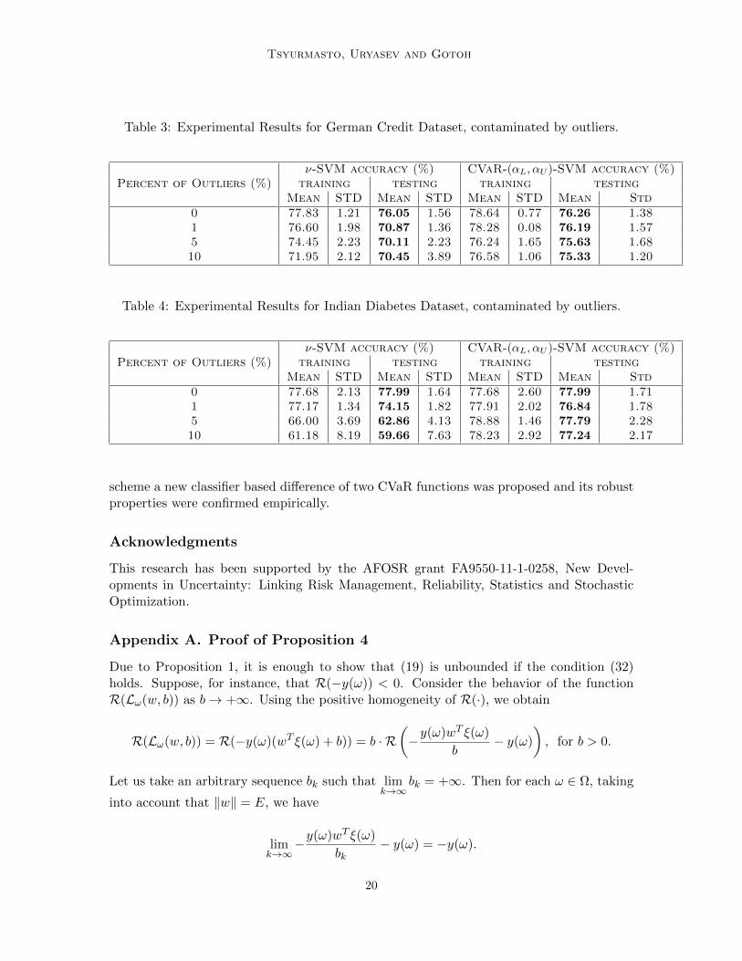
Table 3: Experimental Results for German Credit Dataset, contaminated by outliers.



Table 4: Experimental Results for Indian Diabetes Dataset, contaminated by outliers.



scheme a new classifier based difference of two CVaR functions was proposed and its robustproperties were confirmed empirically.

Acknowledgments

This research has been supported by the AFOSR grant FA9550-11-1-0258, New Devel-opments in Uncertainty: Linking Risk Management, Reliability, Statistics and StochasticOptimization.

Appendix A. Proof of Proposition 4

Due to Proposition 1, it is enough to show that (19) is unbounded if the condition (32)holds. Suppose, for instance, that R(−y(ω)) < 0. Consider the behavior of the functionR(Lω(w, b)) as b→ +∞. Using the positive homogeneity of R(·), we obtain

R(Lω(w, b)) = R(−y(ω)(wT ξ(ω) + b)) = b · R(−y(ω)wT ξ(ω)

b− y(ω)

), for b > 0.

Let us take an arbitrary sequence bk such that limk→∞

bk = +∞. Then for each ω ∈ Ω, taking

into account that ‖w‖ = E, we have

limk→∞

−y(ω)wT ξ(ω)

bk− y(ω) = −y(ω).

20


Table 5: Experimental Results for Ionosphere Dataset, contaminated by outliers.



Table 6: Optimal values of parameters of Linear CVaR-(αL, αu)-SVM.

OPTIMAL PARAMETERS (αL, αU )FOR DIFFERENT % OF OUTLIERS

Data Set 0% 1% 5% 10%αL αU αL αU αL αU αL αU

Liver Disorder 0.3 0.96 0.45 0.9 0.55 0.88 0.5 0.85Heart Disease 0.65 0.94 0.40 0.95 0.65 0.93 0.60 0.95German Credit 0.45 0.95 0.50 0.98 0.60 0.94 0.60 0.90Indian Diabetes 0.45 1 0.4 0.98 0.45 0.95 0.55 0.94

Ionosphere 0.65 0.92 0.40 0.90 0.35 0.97 0.50 0.91

Due to the continuity of R(·), we obtain

limk→∞

R(y(ω)wT ξ(ω)

bk− y(ω)

)= R(−y(ω)) < 0.

Therefore, limb→+∞

R(Lω(w, b)) = limb→+∞

b·R(−y(ω)wT ξ(ω)

b − y(ω))

= −∞, which implies that

(19) is unbounded.Now, suppose thatR(y(ω)) < 0. Applying the same reasoning as for the caseR(−y(ω)) <

0, we obtain

limb→−∞

R(Lω(w, b)) = limb→−∞

R(−y(ω)(wT ξ(ω) + b)) =

limb→−∞

|b| · R(−y(ω)wT ξ(ω)

b+ y(ω)

)= lim

b→−∞|b| · R(y(ω)) = −∞,

which implies that (19) is unbounded and condition minR(−y(ω)),R(y(ω)) ≥ 0 is nec-essary for the existence of an optimal solution of (19).

Appendix B. Proof of Proposition 5

1. Suppose that (w∗, b∗) is an optimal solution of (17) with negative objective value, then(Ew∗

‖w∗‖ ,Eb∗

‖w∗‖

)is an optimal solution of (19) due to Proposition (1). Moreover, the opti-

mal objective value of (19) is negative sinceR(Lω(Ew∗

‖w∗‖ ,Eb∗

‖w∗‖

))= ER

(Lω(w∗,b∗)‖w∗‖

)<

21


Table 7: Optimal values of parameter 1− ν for ν-SVM.

OPTIMAL PARAMETERS νFOR DIFFERENT % OF OUTLIERS

Data Set 0% 1% 5% 10%Liver Disorder 0.80 0.75 0.95 0.95Heart Disease 0.4 0.55 0.55 0.55German Credit 0.55 0.60 0.95 0.95Indian Diabetes 0.60 0.60 0.95 0.95

Ionosphere 0.70 0.75 0.90 0.95

Table 8: Experimental Results for kernel ν-SVM and CVaR-(αL, αr)-SVM.

ν-SVM accuracy (%) CVaR-(αL, αU )-SVM accuracy (%)Data Set training testing training testing

Mean STD Mean STD Mean STD Mean StdLiver Disorder 77.68 2.13 77.99 1.64 77.68 2.60 77.99 1.71Heart Disease 77.17 1.34 73.26 1.82 77.91 2.02 73.75 1.78German Credit 66.00 3.69 69.68 4.13 78.88 1.46 69.96 2.28Indian Diabetes 61.18 8.19 72.97 7.63 78.23 2.92 73.94 2.17

Ionosphere 87.30 4.24 87.30 7.63 78.23 2.92 88.67 2.17

0. Since the difference between the optimization problems (19) and (20) is only ina norm constraint on w, it is enough to show that ‖w‖ = E holds for each optimalsolution (w, b) of (20). To obtain contradiction, suppose that ‖w‖ < E. If w 6= 0, then

R(Lω(Ew‖w‖ ,

Eb‖w‖

))= E‖w‖R

(Lω(w, b)

)< R

(Lω(w, b)

)since E

‖w‖ > 1 and optimal

objective value of (19) is negative. Thus, we obtain contradiction with optimality of(w, b). If w = 0, then an objective value of (20) can be rewritten asR(−y(ω)·b). Since(17) has an optimal solution, then condition minR(−y(ω)),R(y(ω)) ≥ 0 holds due

to Proposition 4. Thus, R(Lω(Ew∗

‖w∗‖ ,Eb∗

‖w∗‖

))< 0 ≤ R

(Lω(w, b)

)= R(−y(ω) · b),

which contradicts an optimality of (w, b).2. Suppose that (w∗, b∗) is an optimal solution of (20) such that w∗ 6= 0. Then it follows

that ‖w∗‖ = E as proved in the first part of this Proposition. Thus, (w∗, b∗) isan optimal solution of (19). Applying Proposition (1), we obtain that (λw∗, λb∗) isoptimal solution of (17) for each λ > 0.

Appendix C. Proof of Proposition 6

1. For short, denote ζ = |R(Lω(w∗, b∗))|. Suppose that (w∗, b∗) is optimal for (17)with negative optimal objective value, then D

ζ (w∗, b∗) is also optimal for (17) andDζ R(Lω(w∗, b∗)) = −D. Then D

ζ (w∗, b∗) is optimal to:

minimizew,b

R(Lω(w, b)

‖w‖

)subject to R(Lω(w, b)) = −D, (41)

22


Optimization problem (41) can be equivalently recast:

minimizew,b

1

2‖w‖2 subject to R(Lω(w, b)) = −D, (42)

Indeed R(−b · y(ω)) ≥ 0 due to Proposition 4, which implies that optimal solutionof (42) satisfies condition w 6= 0. Thus, (w∗, b∗) is optimal for (42). Let us showthat (w∗, b∗) is optimal for (21). To obtain contradiction, suppose that (w∗, b∗) is notoptimal for (21), i.e. R(Lω(w∗, b∗)) < −D, then (w, b) = D

|R(Lω(w,b))|(w∗, b∗) is feasible

for (21) and ‖w‖ < ‖w∗‖, which contradicts the optimality of (w∗, b∗). Thus, (w∗, b∗)is optimal for (21).

2. Suppose that (w∗, b∗) is an optimal solution of (21) and w∗ 6= 0. ThenR(Lω(w∗, b∗)) =−D as proved above. With this fact and positive homogeneity of R(·), the solution(w∗, b∗) is optimal to (41) Then λ(w∗, b∗) is optimal for (17) for each λ > 0.

Appendix D. Proof of Proposition 7

1. Suppose that (w∗, b∗) is an optimal solution of (17) with negative optimal objective

value R(Lω(w∗,b∗)‖w∗‖

)< 0. For short, let us make a notation r∗ = −R

(Lω(w∗,b∗)‖w∗‖

).

Objective of (22) can be rewritten as follows:

1

2‖w‖2 + C · R(Lω(w, b)) =

12‖w‖

2 + C · R(Lω(w,b))‖w‖ ‖w‖, if w 6= 0

R(−b · y(ω)), if w = 0.(43)

Since we have R(−b · y(ω)) ≥ 0 due to Proposition 4, it suffices to consider the casew 6= 0. Optimality of (w∗, b∗) for (17) and positive homogeneity of R(·) implies thatR(Lω(w,b))‖w‖ ≥ R(Lω(w∗,b∗))

‖w∗‖ = −r∗ for each (w, b) ∈ Rn+1, w 6= 0 and we have

1

2‖w‖2 + C · R(Lω(w, b))

‖w‖‖w‖ ≥ 1

2‖w‖2 − Cr∗‖w‖

=1

2(‖w‖ − Cr∗)2 − 1

2C2(r∗)2 ≥ −1

2(Cr∗)2.

(44)

and the lower bound −12(Cr∗)2 in (44) is attained on the point Cr∗

‖w∗‖(w∗, b∗). and

consequently, the point Cr∗

‖w∗‖(w∗, b∗) is optimal for (22).

2. Suppose that (w∗, b∗) is an optimal solution of (22) and w∗ 6= 0. To obtain contradic-tion, suppose that λ(w∗, b∗) is not optimal solution of (17), i.e., there exists a (w, b)such that

R

(Lω(w, b)

‖w‖

)< R

(Lω(w∗, b∗)

‖w∗‖

). (45)

Let r = −R(Lω(w,b))‖w‖ . Then we have

1

2‖w∗‖2 + C · R(Lω(w∗, b∗)) =

1

2‖w∗‖2 + C · R

(Lω(w∗, b∗)

‖w∗‖

)‖w∗‖ >

1

2‖w∗‖2 + C · R(Lω(w, b))

‖w‖‖w∗‖ =

1

2(‖w∗‖ − Cr)2 − 1

2(Cr)2 ≥ −1

2(Cr)2. (46)

23


This implies that Cr‖w‖(w, b) attains a smaller objective value of (22) than (w∗, b∗),

contradicting the optimality of (w∗, b∗).

Appendix E. Proof of Proposition 10

Due to Proposition 1, it is enough to show that (19) has an optimal solution if the condition(33) holds. Suppose that minR(−y(ω)),R(y(ω)) > 0 and prove that (19) has an optimalsolution. First, observe R(Lω(w, b)) is lower semi-continuous with respect to (w, b). (Notethat R(·) is lower semi-continuous and Lω(·, ·) is an affine function). Second, we prove thatif minR(−y(ω)),R(y(ω)) > 0, then lim

b→∞R(Lω(w, b)) = ∞. Let us find, for instance,

limb→+∞

R(Lω(w, b)). Again, applying the positive homogeneity of R(·), we obtain

R(Lω(w, b)) = R(−y(ω)[wT ξ(ω) + b]) = b · R(−y(ω)wT ξ(ω)

b− y(ω)

), for b > 0.

Applying lower semi-continuity of R(·), we obtain

limb→+∞

R(−y(ω)wT ξ

b− y(ω)

)≥ R(−y(ω)) > 0.

Therefore, limb→+∞

R(Lω(w, b)) = ∞. In a similar way, it can be shown that R(y(ω)) > 0

implies limb→−∞

R(Lω(w, b)) =∞.

Now, we show that an optimal solution of (19) exists, if minR(−y(ω)),R(y(ω)) > 0.For each δ > 0 the following optimization problem has an optimal solution

minimizew,b

R(Lω(w, b)) subject to ‖w‖ = E, |b| ≤ δ. (47)

since the lower semi-continuous function R(Lω(w, b)) is minimized over a compact set. De-note by (w∗δ , b

∗δ) an optimal solution of problem (47). If there exists δ > 0, such that

for (w∗δ , b∗δ) and for each (wδ, bδ), wδ ∈ Rn, bδ ∈ R satisfying ‖wδ‖ = E, |bδ| ≥ δ, we

have R(Lω(w∗δ , b∗δ)) ≤ R(Lω(wδ, bδ)), then (w∗δ , b

∗δ) is the optimal solution of (19). To

obtain contradiction, suppose that for each δ > 0 there exists (wδ, bδ), wδ ∈ Rn, bδ ∈R satisfying ‖wδ‖ = E, |bδ| ≥ δ such that R(Lω(wδ, bδ)) < R(Lω(w∗δ , b

∗δ)). We have

R(Lω(w∗δ , b∗δ)) ≤ R(Lω((w∗1, b

∗1)) for each δ ≥ 1 since minimization over a broader feasible

region yields a lower optimal objective value. Therefore, R(Lω(wδ, bδ)) < R(Lω(w∗δ , b∗δ)) ≤

R(Lω(w∗1, b∗1)) for δ ≥ 1. Since lim

δ→∞bδ = ∞ and lim

b→∞R(Lω(w, b)) = ∞ (as we proved

earlier), then limδ→∞R(Lω(wδ, bδ)) = ∞, which contradicts the bound R(Lω(wδ, wδ)) ≤R(Lω(w∗1, b

∗1)) for δ ≥ 1. Thus, we proved that an optimal solution of (19) exists, if

minR(−y(ω)),R(y(ω)) > 0.

24


Appendix F. Example of PSG Meta-Code

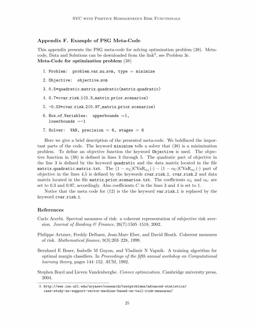
This appendix presents the PSG meta-code for solving optimization problem (38). Meta-code, Data and Solutions can be downloaded from the link3, see Problem 3c.Meta-Code for optimization problem (38)

1. Problem: problem var nu svm, type = minimize

2. Objective: objective svm

3. 0.5*quadratic matrix quadratic(matrix quadratic)

4. 0.7*cvar risk 1(0.3,matrix prior scenarios)

5. -0.03*cvar risk 2(0.97,matrix prior scenarios)

6. Box of Variables: upperbounds =1,

lowerbounds =-1

7. Solver: VAN, precision = 6, stages = 6

Here we give a brief description of the presented meta-code. We boldfaced the impor-tant parts of the code. The keyword minimize tells a solver that (38) is a minimizationproblem. To define an objective function the keyword Objective is used. The objec-tive function in (38) is defined in lines 3 through 5. The quadratic part of objective inthe line 3 is defined by the keyword quadratic and the data matrix located in the filematrix quadratic matrix.txt. The (1 − αL)CVaRαL(·) − (1 − αU )CVaRαU (·) part ofobjective in the lines 4,5 is defined by the keywords cvar risk 1, cvar risk 2 and datamatrix located in the file matrix prior scenarios.txt. The coefficients αL and αU areset to 0.3 and 0.97, accordingly. Also coefficients C in the lines 3 and 4 is set to 1.

Notice that the meta code for (12) is the the keyword var risk 1 is replaced by thekeyword cvar risk 1.

References

Carlo Acerbi. Spectral measures of risk: a coherent representation of subjective risk aver-sion. Journal of Banking & Finance, 26(7):1505–1518, 2002.

Philippe Artzner, Freddy Delbaen, Jean-Marc Eber, and David Heath. Coherent measuresof risk. Mathematical finance, 9(3):203–228, 1999.

Bernhard E Boser, Isabelle M Guyon, and Vladimir N Vapnik. A training algorithm foroptimal margin classifiers. In Proceedings of the fifth annual workshop on Computationallearning theory, pages 144–152. ACM, 1992.

Stephen Boyd and Lieven Vandenberghe. Convex optimization. Cambridge university press,2004.

3. http://www.ise.ufl.edu/uryasev/research/testproblems/advanced-statistics/

case-study-nu-support-vector-machine-based-on-tail-risk-measures/

25

http://www.ise.ufl.edu/uryasev/research/testproblems/advanced-statistics/case-study-nu-support-vector-machine-based-on-tail-risk-measures/

http://www.ise.ufl.edu/uryasev/research/testproblems/advanced-statistics/case-study-nu-support-vector-machine-based-on-tail-risk-measures/


David J Crisp Christopher JC Burges. A geometric interpretation of ν-svm classifiers.Advances in Neural Information Processing Systems 12, 12:244–250, 2000.

Chih-Chung Chang and Chih-Jen Lin. Training ν-support vector regression: theory andalgorithms. Neural Computation, 14(8):1959–1977, 2002.

Olivier Chapelle. Training a support vector machine in the primal. Neural Computation,19(5):1155–1178, 2007.

Ronan Collobert, Fabian Sinz, Jason Weston, and Leon Bottou. Trading convexity forscalability. In Proceedings of the 23rd international conference on Machine learning,pages 201–208. ACM, 2006.

Corinna Cortes and Vladimir Vapnik. Support-vector networks. Machine learning, 20(3):273–297, 1995.

Nello Cristianini and John Shawe-Taylor. An introduction to support vector machines andother kernel-based learning methods. Cambridge university press, 2000.

Darrell Duffie and Jun Pan. An overview of value at risk. The Journal of derivatives, 4(3):7–49, 1997.

Jun-ya Gotoh and Akiko Takeda. A linear classification model based on conditional geo-metric score. Pacific Journal of Optimization, 1:277–296, 2005.

Jun-ya Gotoh, Akiko Takeda, and Rei Yamamoto. Interaction between financial risk mea-sures and machine learning methods. Computational Management Science, pages 1–38,2013a.

Jun-ya Gotoh, Akiko Takeda, and Rei Yamamoto. Interaction between financial risk mea-sures and machine learning methods. Computational Management Science, 2013b.

R Horst and Ng V Thoai. Dc programming: overview. Journal of Optimization Theory andApplications, 103(1):1–43, 1999.

Reiner Horst and Hoang Tuy. Global optimization: Deterministic approaches. Springer,2003.

Reiner Horst, Panos M Pardalos, and Nguyen Van Thoai. Introduction to global optimiza-tion. Kluwer Academic Pub, 2000.

Philippe Jorion. Value at risk: the new benchmark for controlling market risk, volume 2.McGraw-Hill New York, 1997.

K-R Muller, Sebastian Mika, Gunnar Ratsch, Koji Tsuda, and Bernhard Scholkopf. Anintroduction to kernel-based learning algorithms. Neural Networks, IEEE Transactionson, 12(2):181–201, 2001.

Fernando Perez-Cruz, Jason Weston, DJL Herrmann, and B Scholkopf. Extension of the nu-svm range for classification. NATO SCIENCE SERIES SUB SERIES III COMPUTERAND SYSTEMS SCIENCES, 190:179–196, 2003.

26


R Tyrrell Rockafellar and Stan Uryasev. The fundamental risk quadrangle in risk man-agement, optimization and statistical estimation. Surveys in Operations Research andManagement Science, 18(1):33–53, 2013.

R Tyrrell Rockafellar and Stanislav Uryasev. Optimization of conditional value-at-risk.Journal of risk, 2:21–42, 2000.

Bernhard Scholkopf, Alex J Smola, Robert C Williamson, and Peter L Bartlett. Newsupport vector algorithms. Neural computation, 12(5):1207–1245, 2000.

Akiko Takeda and Masashi Sugiyama. ν-support vector machine as conditional value-at-riskminimization. In Proceedings of the 25th international conference on Machine learning,pages 1056–1063. ACM, 2008.

Pham Dinh Tao et al. The dc (difference of convex functions) programming and dca revisitedwith dc models of real world nonconvex optimization problems. Annals of OperationsResearch, 133(1-4):23–46, 2005.

Peter Tsyurmasto, Michael Zabarankin, and Stan Uryasev. Value-at-risk support vectormachine: Stability to outliers. 2013.

Vladimir Vapnik. The nature of statistical learning theory. springer, 1999.

27

Documents

Support Vector Classi cation with Positive … with Positive Homogeneous Risk Functionals In addition, the principle of the structural risk minimization does not mention how it treats