Supply Function Competition, Private Information, andMarket Power: A Laboratory Study

Anna Bayona,∗Jordi Brandts,†and Xavier Vives‡§

July 2016

Abstract

In the context of supply function competition with private information, we test in thelaboratory whether—as predicted in Bayesian equilibrium—costs that are positively correl-ated lead to steeper supply functions and less competitive outcomes than do uncorrelatedcosts. We find that the majority of subjects bid in accordance with the equilibrium pre-diction when the environment is simple (uncorrelated costs treatment) but fail to do soin a more complex environment (positively correlated costs treatment). Although we findno statistically significant differences between treatments in average behaviour and out-comes, there are significant differences in the distribution of supply functions. Our resultsare consistent with the presence of sophisticated agents that on average best respond to alarge proportion of subjects who ignore the correlation among costs. Experimental welfarelosses in both treatments are higher than the equilibrium prediction owing to a substantialdegree of productive inefficiency.

Keywords: divisible good auction, generalised winner’s curse, correlation neglect, elec-tricity market

JEL Codes: C92, D43, L13

∗ESADE Business School.†Institut d’Anàlisi Econòmica (CSIC) and Barcelona GSE.‡IESE Business School.§We thank José Apesteguia, Maria Bigoni, Colin Camerer, Enrique Fatas, Dan Levin, Cristina Lopez-Mayan,

Margaret Meyer, Rosemarie Nagel, Stanley Reynolds, Albert Satorra, Arthur Schram, and Jack Stecher foruseful comments and discussions. Anna Bayona acknowledges the financial support from Banc de Sabadell.Jordi Brandts acknowledges financial support from the Spanish Ministry of Economics and Competitiveness(Grant ECO2014-59302-P) and the Generalitat de Catalunya (AGAUR Grant 2014 SGR 510). Xavier Vivesacknowledges financial support of the Spanish Ministry of Economics and Competitiveness (Grant ECO2015-63711-P) and the Generalitat de Catalunya (AGAUR Grant 2014 SGR 1496). The usual disclaimers apply.

1

1 Introduction

We design a laboratory experiment which captures the complexity of the bidding and inform-ation environments which are representative of the real-world markets characterised by com-petition in schedules such as wholesale electricity markets, markets for pollution permits, aswell as liquidity and Treasury auctions.1 We provide experimental evidence of behaviour andoutcomes in a market where each seller has incomplete information about her costs, receives aprivate signal, and competes in supply functions. The aim of our experiment is to study therelationship between information frictions and market power, and to examine the implicationsof the complexity of the environment: uncorrelated costs versus positively correlated costs.

We consider a market where firms compete in terms of supply functions (see Klemperer andMeyer 1989) and with incomplete cost information (Vives 2011). The latter paper finds that, ina unique linear Bayesian equilibrium, private information with cost correlation generates marketpower that exceeds the full-information benchmark.2 When costs are positively correlated, themodel predicts that the supply function’s slope is steeper and the intercept is lower leading tohigher expected market prices and profits than when costs are uncorrelated. The mechanismthat explains these results can be stated as follows. A seller receives a private signal that isinformative about her random costs. A fully rational seller who is strategic must also realisethat, when costs are positively correlated, a high price conveys the information that costs arehigh; therefore, to protect herself from adverse selection, she should compete less aggressivelythan if costs were uncorrelated. So if all sellers are fully rational then the combination of privateinformation and strategic behaviour leads to greater market power when costs are correlatedthan when they are uncorrelated. The mechanism that relates higher cost correlation to increasedmarket power is connected to a generalised version of the winner’s curse (Ausubel et al. 2014)that extends this concept to multi-unit demand auctions.3

The experimental design is as follows. We employ a between-subjects experimental designwith two treatments that only differ in the correlation among costs.4 In each treatment, subjectswere randomly assigned to independent groups of twelve subjects, each comprising four marketsof three sellers. Within each group, we applied random matching between rounds in order toretain the theoretical model’s one-shot nature. The buyer was simulated, and subjects wereassigned the role of sellers. Subjects received a private signal about the uncertain cost and

1The following papers argue for the importance of demand or cost uncertainty among bidders that competein schedules: wholesale electricity markets (Holmberg and Wolak 2015); liquidity auctions (Cassola et al. 2013);Treasury auctions (Keloharju et al. 2005); carbon dioxide emission permits (Lopomo et al. 2011).

2The supply function equilibrium with uncorrelated costs coincides with the full-information equilibrium sincesellers do not learn about cost uncertainty from prices.

3The connection is established in the Related Literature section.4In a between-subjects design participants are either part of the control group or the treatment group but

cannot participate in both.

2

were then asked to submit a (linear) supply function. As in the theoretical model, and incontrast to most of the experimental literature, we used a normally distributed informationstructure that well approximates the distribution of values in naturally occurring environments.After all decisions had been made, the uniform market price was calculated and each subjectreceived detailed feedback about her own performance, the market price, and the behaviour andperformance of rivals in the same market. At the end of the experiment, we administered apost-experiment questionnaire that asked about participant’s demographic information, biddingbehaviour, and understanding of the game. Subjects were given incentives that incorporatedboth fixed and variable components, where the variable component reflected the individualparticipant’s performance during the game.

Our experimental data are in line with some of the theoretical predictions. First, we con-firm that average behaviour in the uncorrelated costs treatment closely matches the theoreticalprediction in the experiment’s early stages and that, over time, the average supply functiontends even further toward the equilibrium supply function. This finding is important becausethe uncorrelated costs treatment yields a benchmark against which to compare behaviour in thepositively correlated costs treatment. Second, we find that the features of the equilibrium thatare common to both treatments are observed in the data. In particular, we observe that thesupply function’s intercept is increasing in a bidder’s signal realisation. This result is consist-ent with subjects understanding that a higher signal implies a higher average intercept of themarginal cost, which means they should set a higher ask price for the first unit offered and thisleads, in turn, to a higher supply function intercept. We observe also that the supply function’sslope is unrelated to the signal received.

Analysing the distribution of individual choices, we find that the cumulative distributionof supply function slopes in the positively correlated costs treatment first order stochasticallydominates the cumulative distribution of slopes in the uncorrelated costs treatment, both in thefirst and last five rounds (in a stronger way in the latter). This result shows that differencesin behaviour between treatments are consistent with the direction predicted by the theoreticalmodel. However, we cannot reject the hypothesis that average supply functions are the samein both treatments. In the positively correlated costs treatment we observe that the averagesupply function is substantially flatter and has a higher intercept than predicted by the equilib-rium, which is consistent with subjects being too strongly guided by the signal received. Thisdivergence persists even as subjects gain bidding experience.

In terms of experimental outcomes, we also find differences (albeit insignificant ones) betweentreatments with regard to market prices, profits, and efficiency of the allocations. However, wedo not find the predicted differences in market power between the two treatments. In thepositively correlated costs treatment, bidders forgo a large percentage of profits—an outcometypical of auctions where bidders ignore the adverse effects of correlation among costs. Moreover,

3

experimental welfare losses in both treatments are larger than predicted by the equilibriumowing to the considerable extent of productive inefficiency. These results suggest that subjectsin the positively correlated costs treatment fall prey to the generalised winner’s curse and, asa result, compete too aggressively in comparison with the equilibrium prediction. The greaterheterogeneity in behaviour in the positively correlated (than in the uncorrelated) costs treatmentmerits further exploration.

We offer a detailed analysis of behaviour that proceeds in three parts. First, in each treat-ment we analyse theoretically subjects’ strategic incentives. We remark that the environmentthat we study is complex both in terms of the information setting (the combined uncertaintyregarding cost and private signal) and the market structure (competition in supply functionsand transaction costs which vary with quantity sold). The positively correlated cost treatmentadds a further layer of complexity since the market price is informative about a seller’s cost;hence the equilibrium logic requires subjects to form not only correct beliefs about the eco-nomic environment but also correct higher-order beliefs. In other words, the equilibrium of thepositively correlated costs treatment requires that sellers believe that other sellers are taking ad-vantage of the correlation structure, that they believe that everyone believes this, that everyonebelieves that everyone believes this... We find that a (sophisticated) subject in our positivelycorrelated costs treatment who best responds to the rivals’ average choices has an incentiveto bid a supply function between the equilibrium of the uncorrelated costs treatment and theequilibrium of the positively correlated costs treatment. It follows that behaviour and outcomesbetween treatments (and for different subject types—namely, sophisticated types capable of bestresponding and naïve who fall prey to the generalised winner’s curse—) are less differentiatedthan predicted by the equilibrium (which assumes that all bidders are fully rational).

The second part of our analysis takes a descriptive approach to organising, via cluster ana-lysis, the observed heterogeneity in individual-level behaviour; we then compare the clustersso derived to the various theoretical benchmarks. We use average behaviour in blocks of fiverounds. In the uncorrelated costs treatment, we identify two clusters. One cluster assembleschoices that are close to the equilibrium and theoretical best response to the average choice; thiscluster includes 58% of the subjects in the first five rounds of bidding, a proportion that increasesto 72% in the last five rounds. The other cluster groups subjects whose supply functions aresteeper and have a lower intercept than the equilibrium of the uncorrelated costs treatment; thiscluster includes 42% and 28% of the subjects in (respectively) the first and last five rounds. Inthe positively correlated costs treatment we identify three clusters. One cluster groups subjectswhose supply functions are close to the benchmark for subjects who fall prey to the generalisedwinner’s curse, which includes 58% of the subjects in the first five rounds of bidding and 50%in the last five rounds. Another cluster gathers subjects whose bidding behaviour is not incon-sistent with sophisticated behaviour in the sense that their supply functions are close to the

4

theoretical best response to the average supply function; this cluster includes 36% (respectively42%) of subjects in the first (respectively last) five rounds of bidding. Given the complexity ofthe bidding environment, it is interesting to find a substantial number of subjects whose beha-viour approximates the average best response. The third derived cluster groups the remainingsubjects, who bid a steep supply function with a low intercept (6% and 8% of subjects in thefirst and last five rounds, respectively). Although there are few treatment differences in averagebehaviour there are substantial differences in the distributions of individual behaviour. Theseare driven by the two treatments’ different levels of strategic complexity, which lead to theidentification of distinct types of subjects (naïve and sophisticated) in each treatment. Notice,however, that even with a substantial percentage of subjects whose behaviour approximates theaverage best response only moves the aggregate behaviour slightly away from the uncorrelatedcosts treatment.

Finally, we analyse how behaviour changes across rounds and find treatment-based dif-ferences in the determinants of the evolution of behaviour. In particular, the best-responsedynamics factor figures more prominently in the uncorrelated than in the positively correlatedcosts treatment, whereas imitation of the best plays a smaller role in the uncorrelated than inthe positively correlated costs treatment. In each treatment, both imitation of the average andreinforcement learning are important factors in explaining the evolution of behaviour acrossrounds. The combination of these determinants, the initial conditions and strategic complexityexplains why behaviour evolves toward the equilibrium in the uncorrelated costs treatment butnot in the positively correlated costs treatment.

The rest of our paper is organised as follows. We review the related literature in Section 2and explain the theoretical model in Section 3. Section 4 describes the experimental design,after which Section 5 presents our main results. In Section 6 we analyse in detail the behaviourobserved during our experiment. We conclude in Section 7. (The experiment’s instructions maybe found in Appendix C.)

2 Related Literature

Our experimental paper studies competition in supply schedules within an information envir-onment that includes both positively correlated costs and uncorrelated costs. This environmentis reminiscent of the one described in Goeree and Offerman (2003), who also use normally dis-tributed values and error terms. However, their paper compares behaviour in cases of commonversus uncorrelated private values in a single-unit, second-price auction whereas ours comparesbehaviour in cases of correlated versus uncorrelated costs in a supply function, uniform priceauction.

With respect to the competition environment, some early experiments used bid functions in

5

auctions with incomplete information (e.g., Selten and Buchta 1999), but few laboratory exper-iments have sought to analyse, as we do, competition in supply functions. Exceptions includethe work of Bolle et al. (2013), who focus on testing predictions of Supply Function Equi-librium concept, as well as Brandts et al. (2014), whose paper compares testable predictionsmade by various models of how pivotal suppliers affect supply function bidding. In contrast,our experiment focuses on a framework in which market power is driven by a small number offirms, increasing marginal costs, and private information about costs. Outside the laboratory,Hortaçsu and Puller (2008) empirically evaluate strategic bidding behaviour in multi-unit auc-tions using data from the Texas electricity market. These authors find evidence that large firmsbid according to the theoretical benchmark while smaller firms deviate significantly from thatbenchmark.

To the best of our knowledge, ours is the first laboratory experiment to test the relationshipbetween informational frictions and market power in the context of supply function competition.Because of similarities in the information environment, our results are related to findings in theliterature on the winner’s curse in single unit auctions where a savvy bidder avoids biddingaggressively because “winning” conveys the news that her signal was the highest in the mar-ket. A prevalent, consistent, and robust phenomenon in single-unit auctions featuring common(or correlated) values (Kagel and Levin 1986; Goeree and Offerman 2003; Kagel and Levin(forthcoming)) and where bidders ignore the adverse selection problem. However, the analogybetween the winner’s curse with competition in supply functions and with single-unit auctionsapplies with respect to adverse selection but not necessarily with respect to market power. Inessence, our results are more closely related to the generalised winner’s curse (Ausubel et al.2014) which reflects that “winning” a larger quantity is worse news than “winning” a smallerquantity because the former implies a higher expected cost for the bidder (where bidders aresellers). In our environment a seller that faces a high price should think that it is likely thatcosts of her rivals are high and this is news that her own costs are also high because of thepositive correlation. The result is that the seller should moderate her offer and this induces thesupply function to be steeper. Therefore, rational bidders refrain from competing too aggress-ively. We find evidence of the generalised winner’s curse in a multi-unit, divisible-good auctionwith interdependent values.

The market structure in our setup is reminiscent of multi-unit uniform price auctions, forwhich there is evidence of demand reduction—in demand auctions characterised by independentprivate values and an indivisible good—both experimentally (Kagel and Levin 2001) and in thefield (List and Lucking-Reiley 2000; Levin 2005; Engelbrecht-Wiggans et al. 2005; Engelbrecht-Wiggans et al. 2006). Unlike this literature, our paper addresses a uniform-price auction withinterdependent values and a divisible good. The experiment we conduct is also related to thatof Sade et al. (2006), who test the theoretical predictions of a divisible-good, multi-unit auction

6

model under different auction designs; they report some inconsistencies between the theoreticalequilibrium strategies and actual experimental behaviour.

There is also an experimental literature on “correlation neglect” in various strategic con-texts. Those contexts include bilateral negotiations (Samuelson and Bazerman 1985), tradewith adverse selection (Holt and Sherman 1994), social learning (Weizsacker 2010), auctionswith toeholds (Georganas and Nagel 2011), voting (Esponda and Vespa 2014; Levy and Razin2015), and belief formation (Enke and Zimmermann 2013; Koch and Penczynski 2015). Ourresults are consistent also with these experimental findings in that a substantial proportion ofour subjects ignore correlation among costs and hence its adverse effects.

The detailed analysis of our results echoes the analysis of other strategic games with privateinformation; examples include Carrillo and Palfrey (2011) as well as Brocas et al. (2014), whoconduct a similar cluster analysis. Both of those papers report that (a) a large proportionof subjects behave just as in the equilibrium where subjects play simple but strategic private-information games yet (b) this proportion declines markedly with increasing strategic complexityof the game. Charness and Levin (2009) attribute the origin of the winner’s curse to boundedrationality since individuals have difficulties thinking contingently about future events. Thisbehavioural bias is also likely to apply to the subjects of our experiment since the equilibriumof the positively correlated costs treatment requires that a bidder thinks contingently aboutthe relationship between the market price and unit costs. Furthermore, the evolution of choicesacross rounds that we observe is related to the work of Huck et al. (1999) and Bigoni andFort (2013), who analyse learning in a Cournot setting. Much as in those papers, our ownresults indicate that learning is a composite process that involves elements of both adaptiveand reinforcement learning—despite the greater complexity of our environment (in which sub-jects set supply functions with incomplete information rather than choosing quantities with fullinformation).

The complexity of the our baseline model makes the comparison of our results to extantbehavioural models somewhat difficult. Eyster and Rabin (2005) propose the cursed equilib-rium concept, whereby players incorrectly assess the relationship between rivals’ strategies andtheir own private information. In our setting, then, a player in the positively correlated coststreatment would be “fully cursed” if she ignored the information that price conveys about costs.Except for the two extreme cases in which all players are fully cursed or all players are fully ra-tional, there are several analytical difficulties associated with computing the cursed equilibriumin our complex setting; we therefore refrain from further relating our results to that notion. Analternative equilibrium concept that could explain our choices would be the quantal responseequilibrium (QRE), which assumes that the probability of any strategy is increasing in thestrategy’s expected payoff and rationalises the idea that players make mistakes. However, thecalculation of the QRE for our baseline model is beyond the scope of this paper. Finally, a

7

nonequilibrium potential explanation of our results could be given by the level-k model of stra-tegic thinking (Nagel 1995; Crawford and Iriberri 2007). We do not formally apply the level-kmodel to describe our experimental choices for the following reasons. First, if we define level-0 asthe equilibrium behaviour of the uncorrelated costs treatment then we cannot explain the het-erogeneity that we observe in the uncorrelated costs treatment. For other plausible definitions oflevel-0, the theoretical level-k predictions do not correspond to observed peaks that we observein the distribution of choices. Second, the various levels are not sufficiently differentiated toenable clear identification of a subjects’ degree of strategic thinking. Given these limitations, wefocus on analysing the theoretical and empirical distribution of best replies, an approach thatyields a categorisation of subjects into clusters: those who are naïve (subjects that fall prey tothe generalised winner’s curse) and sophisticated (responding best to the average strategy ofrivals).

3 Theoretical Background

We use the framework of Vives (2011) to guide our experimental design. There are a finitenumber n of sellers who compete simultaneously in a uniform price auction, and each sellersubmits a supply function. Seller i’s profits can be written as

πi = (p− θi)xi −λ

2x2i , (1)

where xi are the units sold, θi denotes a random cost parameter, p is a uniform market price,and λ > 0 represents a parameter that measures the level of transaction costs. The market-clearing condition allows us to find the uniform market price p. The (random) cost parameter θiis normally distributed as θi ∼ N(θ, σ2

θ). The demand is inelastic and equal to q.The information structure is as follows. A seller does not know the value of the cost shock θi

before setting her supply schedule, and she receives a signal si = θi + εi for which the errorterm is distributed as εi ∼ N(0, σ2

ε ). Sellers’ random cost parameters may be correlated, withcorr(θi, θj) = ρ for i 6= j. When ρ = 1 the model is equivalent to a common costs model,when ρ = 0 to an uncorrelated costs model, and when 0 < ρ < 1 to a correlated costs model.Error terms are uncorrelated either among themselves or with the random cost shocks. In ourexperiment, the treatment variable is the correlation ρ among costs.

Since the payoff function is quadratic and since the information structure is normally dis-tributed, we focus on linear supply schedules. Linear supply functions are a reasonable approx-imation of the types of supply functions submitted by bidders in real markets.5 Given the signal

5See, for example, Baldick et al. (2004).

8

received, a strategy for seller i is to submit a price-contingent schedule, X(si, p), of the form

X(si, p) = b− asi + cp. (2)

Thus the seller’s supply function is determined by the three coefficients (a, b, c). We interpretthese coefficients is as follows: a is a bidder’s response to the private signal; b is the fixed partof the supply function’s intercept f = b− asi; and c is the supply function’s slope.

Vives (2011) finds a unique supply function equilibrium and describes how the equilibriumparameters (a, b, c) depend on the information structure (θ, σ2

θ , σ2ε , ρ) and on the market structure

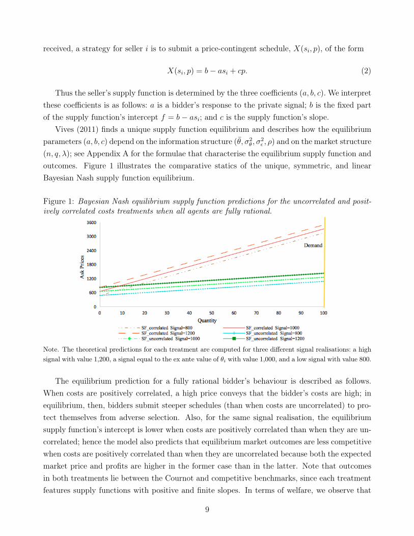
(n, q, λ); see Appendix A for the formulae that characterise the equilibrium supply function andoutcomes. Figure 1 illustrates the comparative statics of the unique, symmetric, and linearBayesian Nash supply function equilibrium.

Figure 1: Bayesian Nash equilibrium supply function predictions for the uncorrelated and posit-ively correlated costs treatments when all agents are fully rational.

Note. The theoretical predictions for each treatment are computed for three different signal realisations: a highsignal with value 1,200, a signal equal to the ex ante value of θi with value 1,000, and a low signal with value 800.

The equilibrium prediction for a fully rational bidder’s behaviour is described as follows.When costs are positively correlated, a high price conveys that the bidder’s costs are high; inequilibrium, then, bidders submit steeper schedules (than when costs are uncorrelated) to pro-tect themselves from adverse selection. Also, for the same signal realisation, the equilibriumsupply function’s intercept is lower when costs are positively correlated than when they are un-correlated; hence the model also predicts that equilibrium market outcomes are less competitivewhen costs are positively correlated than when they are uncorrelated because both the expectedmarket price and profits are higher in the former case than in the latter. Note that outcomesin both treatments lie between the Cournot and competitive benchmarks, since each treatmentfeatures supply functions with positive and finite slopes. In terms of welfare, we observe that

9

the equilibrium allocation is inefficient due to distributive inefficiency. Because demand is in-elastic, there is no aggregate inefficiency at the equilibrium allocation. At this allocation, sellerssupply quantities that exhibit too little dispersion vis-à-vis the efficient benchmark, which isreflected in the ex-ante expected deadweight loss at the equilibrium allocation (it is defined asthe difference between expected total surplus at the efficient and equilibrium allocations).

The comparative statics of the unique Bayesian Nash equilibrium—which assumes that allsellers are fully rational and ex ante symmetric—allow us to derive the testable predictionsencapsulated by the six hypotheses listed here as (A)–(F). These hypotheses focus on the model’sgeneral predictions and on the comparative statics with respect to the correlation among costs,since ρ is our treatment variable.

(A) In each treatment, the supply function slope is positive and unrelated to a bidder’s signalrealisation.

(B) In each treatment, the supply function intercept is nonzero and increasing in a bidder’ssignal realisation.

(C) The supply function is steeper in the positively correlated costs treatment than in theuncorrelated costs treatment.

(D) For a given signal realisation, the supply function’s intercept is lower in the positive cor-related costs treatment than in the uncorrelated costs treatment; therefore, the expectedsupply function intercept is lower in the positive correlated costs treatment than in theuncorrelated costs treatment.

(E) The expected market price and profits are larger in the positively correlated costs treatmentthan in the uncorrelated costs treatment.

(F) The expected deadweight loss is larger in the uncorrelated costs treatment than in thepositively correlated costs treatment.6

If subjects ignore the correlation among costs and thus do not understand that winninga larger quantity is worse news (when costs are positively correlated) than winning a smallerquantity, then those subjects fall prey to the winner’s curse in the context of a multi-unit auctionwith interdependent values. (This phenomenon was termed the generalised winner’s curse byAusubel et al. 2014.) Therefore, the benchmark for subjects who fall prey to the generalisedwinner’s curse is the equilibrium of the uncorrelated costs treatment. If all subjects were tofall prey to that curse then we should expect behaviour and market outcomes in both of our

6This claim follows from the chosen constellation of experimental parameters (see Table 2 in Section 4),although the theoretical prediction asserts that the expected deadweight loss can either increase or decreasewith the correlation among costs.

10

experimental treatments to be indistinguishable, in which case hypotheses (C)–(F) might notbe hold.7 The hypotheses just listed pertain to point estimates and expected behaviour, yetexperimental variation in behaviour and outcomes may also be of interest. We explore theseissues in Section 5.

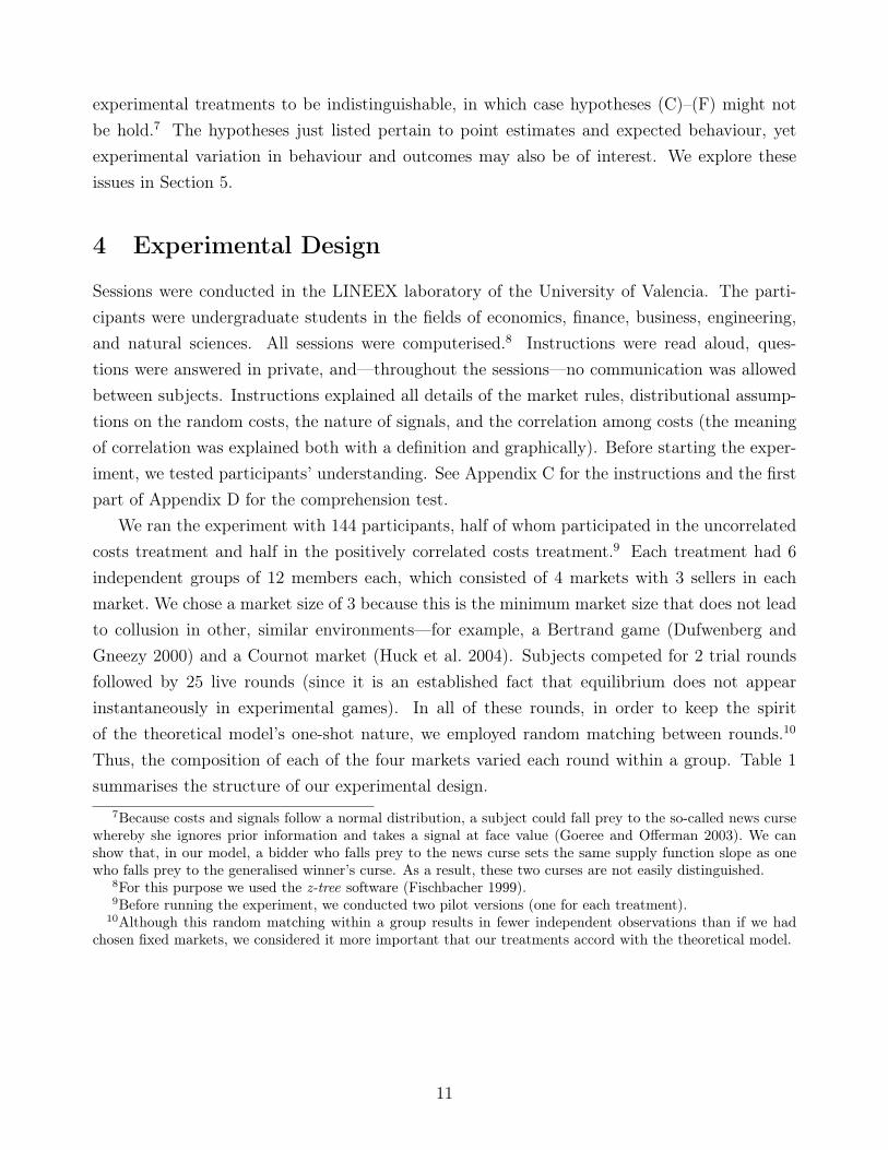
4 Experimental Design

Sessions were conducted in the LINEEX laboratory of the University of Valencia. The parti-cipants were undergraduate students in the fields of economics, finance, business, engineering,and natural sciences. All sessions were computerised.8 Instructions were read aloud, ques-tions were answered in private, and—throughout the sessions—no communication was allowedbetween subjects. Instructions explained all details of the market rules, distributional assump-tions on the random costs, the nature of signals, and the correlation among costs (the meaningof correlation was explained both with a definition and graphically). Before starting the exper-iment, we tested participants’ understanding. See Appendix C for the instructions and the firstpart of Appendix D for the comprehension test.

We ran the experiment with 144 participants, half of whom participated in the uncorrelatedcosts treatment and half in the positively correlated costs treatment.9 Each treatment had 6independent groups of 12 members each, which consisted of 4 markets with 3 sellers in eachmarket. We chose a market size of 3 because this is the minimum market size that does not leadto collusion in other, similar environments—for example, a Bertrand game (Dufwenberg andGneezy 2000) and a Cournot market (Huck et al. 2004). Subjects competed for 2 trial roundsfollowed by 25 live rounds (since it is an established fact that equilibrium does not appearinstantaneously in experimental games). In all of these rounds, in order to keep the spiritof the theoretical model’s one-shot nature, we employed random matching between rounds.10

Thus, the composition of each of the four markets varied each round within a group. Table 1summarises the structure of our experimental design.

7Because costs and signals follow a normal distribution, a subject could fall prey to the so-called news cursewhereby she ignores prior information and takes a signal at face value (Goeree and Offerman 2003). We canshow that, in our model, a bidder who falls prey to the news curse sets the same supply function slope as onewho falls prey to the generalised winner’s curse. As a result, these two curses are not easily distinguished.

8For this purpose we used the z-tree software (Fischbacher 1999).9Before running the experiment, we conducted two pilot versions (one for each treatment).

10Although this random matching within a group results in fewer independent observations than if we hadchosen fixed markets, we considered it more important that our treatments accord with the theoretical model.

11

Table 1: Experimental design.

In the second part of Appendix D we reproduce the screenshots used for running the ex-periment. In each round, all subjects received a private signal and were subsequently asked tochoose two ask prices : one for the first unit offered and one for the second. We then used thesetwo ask prices to construct a linear supply schedule, which was shown in the form of a graph oneach subject’s screen. The participant could then revise the ask prices several times until shewas satisfied with her decision. The buyer was simulated.

Once all supply schedules had been submitted, each bidder received feedback on the uniformmarket price, her own performance (with regard to revenues, production costs, transaction costs,units sold, and profits), the performance of the other two market participants (units sold, profits,and supply functions), and the values of the random variables drawn (her own cost and thecosts of the other two participants in the same market).11 Participants were allowed to consultthe history of their own performance. Other experiments have shown that feedback affectsbehaviour in the laboratory. In a Cournot game, for example, Offerman et al. (2002) reportthat different feedback rules can result in outcomes that range from competitive to collusive.Given the complexity of our experiment, we maximised the feedback given after each round inorder to maximise the potential learning of participants. After each participant had checkedher feedback, a new round of the game would start. Note that, in each market and for eachround, we generated three random unit costs from a multivariate normal distribution. Also, ineach round and for each participant, the unit costs and signals were independent draws fromprevious and future rounds.

Conducting the experiment required us to specify numerical values for the theoretical model’sparameters; see Table 2. For this purpose we used three criteria: (i) the existence of a uniqueequilibrium; (ii) sufficiently differentiated behaviour and outcomes between the two treatments;and (iii) reduction of computational demands placed on participants. It is important to bear inmind that ρ = 0 for the uncorrelated costs (control) treatment whereas ρ = 0.6 for the positivelycorrelated costs treatment.12 Refer to Appendix B for the equilibrium supply function and

11Subjects did not receive feedback on the signal received because that would not be expected to occur inreality. That is: after trading, firms may observe the actual costs of competitors but are unlikely to observe theprivate signals competitors had received at the time of their decisions.

12We would have preferred to set a higher correlation among unit costs so that our predictions would bemaximally differentiated. Yet inelastic demand reduces the range for which a unique equilibrium exists, and

12

outcomes (based on Table 2’s experimental parameters) and for a statistical description of thedistribution of random costs and errors used in the experiment.

Table 2: Experimental parameters.

We imposed certain market rules, which were inspired by the theoretical model and facil-itated implementation of the experiment. First, we asked each seller to offer all 100 units forsale. Second, we asked sellers to construct a nondecreasing and linear supply function. Third,ask prices had to be nonnegative. Fourth, we told bidders that the simulated buyer would notpurchase any unit at a price higher than 3,600; this price cap was imposed in order to limitthe potential gains of sellers in the experimental sessions. Although the price cap was not partof the theoretical model, we chose a value high enough to preclude distortion of equilibriumbehaviour. The only difference between treatments was the correlation among costs and hencethe distribution of random costs and signals.

At the end of the experiment, participants completed a questionnaire (see Appendix E) thatrequested personal information and asked questions about the subject’s reflections after playingthe game. Once the questionnaire was completed, each participant was paid in private.

As for incentives, each participant started with 50,000 experimental points.13 During theexperiment, subjects won or lost points. At the end of the experiment, points were exchangedfor euros at the rate of 10,000 experimental points per euro. In addition, each subject receiveda 10 euros show-up fee. The payments ultimately made to subjects ranged from 10 to 27.8 eurosand averaged 20.8 euros. Each session lasted between two and three hours.

5 Experimental Results

We present our results in three sections. In Section 5.1 we provide an analysis of experimentalbehaviour (supply functions) and in Section 5.2 we analyse experimental outcomes (marketprice and profits) and efficiency of allocations. Section 5.3 addresses trends of behaviour and

ρ = 0.6 was the highest correlation that satisfied our implementation criteria. Inelastic demand was stipulatedin order to simplify the participants’ computations.

13These points were equivalent to 5 euros.

13

outcomes across rounds. Throughout the section, we evaluate Hypotheses (A)–(F) formulatedin Section 3. Appendix G conducts a robustness test of our main experimental results using apanel data approach.

We shall discuss the experimental results in terms of the inverse supply function, since itcorresponds to how participants made their decisions. From any participant’s two-dimensionaldecision, (AskPrice1 ,AskPrice2 ), we can infer the slope and intercept of each participant’sinverse supply function, p = f + cX(si, p). The inverse supply function slope is c, where c =

AskPrice2 − AskPrice1 and the intercept is f , defined as f = AskPrice1 − c. The coefficientsof the inverse supply function are related to the coefficients of equation (2)’s supply function asfollows: b = −b

c; a = a

c; c = 1

cfor c 6= 0; the inverse supply function’s intercept is f = b + asi.

We will omit the modifier “inverse” and refer simply to “the supply function”. We shall useInterceptPQ as the empirical counterpart of f and SlopePQ as the empirical counterpart of c.Our graphs plot the supply function in the usual (Quantity ,AskPrice) space.14

5.1 Analysis of experimental behaviour: supply functions

We first present evidence of the most general testable predictions of the theoretical model thatare common in both treatments. In Section 3 we saw the theoretical framework predictingthat, in both treatments, the supply function slope should be independent of the signal receivedwhereas the supply function intercept should increase with the signal realisation. The latterprediction reflects that a higher signal implies a higher average intercept of the marginal costand so the bidder should set a higher ask price for the first unit offered, leading to a highersupply function intercept.

In each treatment, we find that the average supply function intercept increases with thesignal in each decile. In contrast, the supply function slope remains approximately constant ineach signal decile in either treatment. Furthermore, a regression of the supply function intercepton signal yields a coefficient of 0.856 with p = 0.000 in the uncorrelated costs treatment and acoefficient of 0.926 with p = 0.000 in the positively correlated costs treatment; while a regressionof the supply function slope on signal yields an insignificant coefficient (with p = 0.703 in theuncorrelated costs treatment and with p = 0.655 in the positively correlated costs treatment).15

Figure 2 illustrates the average supply function slope and intercept for each signal decile usingall the choices from both treatments.

14Note that a steep supply function in the (Quantity ,AskPrice) space has a high c and a low c.15The unit of observation for the regressions reported is the group across rounds. In each treatment there are

150 observations: 6 groups over the course of 25 rounds.

14

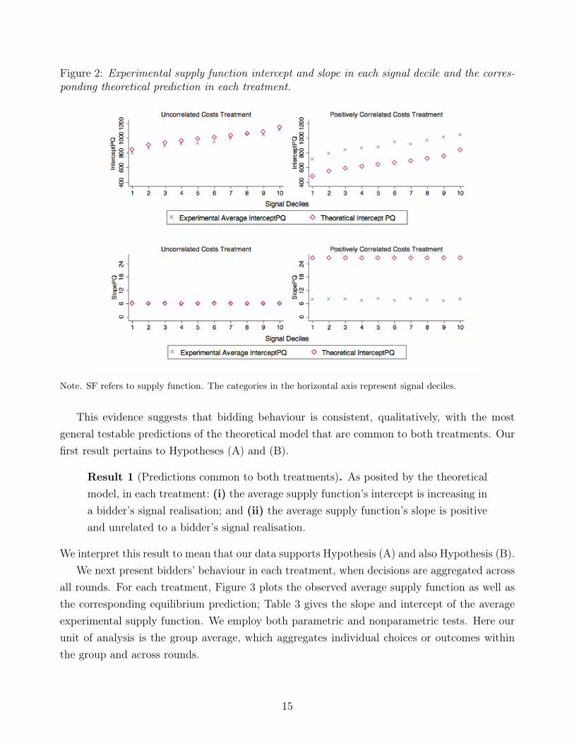
Figure 2: Experimental supply function intercept and slope in each signal decile and the corres-ponding theoretical prediction in each treatment.

Note. SF refers to supply function. The categories in the horizontal axis represent signal deciles.

This evidence suggests that bidding behaviour is consistent, qualitatively, with the mostgeneral testable predictions of the theoretical model that are common to both treatments. Ourfirst result pertains to Hypotheses (A) and (B).

Result 1 (Predictions common to both treatments). As posited by the theoreticalmodel, in each treatment: (i) the average supply function’s intercept is increasing ina bidder’s signal realisation; and (ii) the average supply function’s slope is positiveand unrelated to a bidder’s signal realisation.

We interpret this result to mean that our data supports Hypothesis (A) and also Hypothesis (B).We next present bidders’ behaviour in each treatment, when decisions are aggregated across

all rounds. For each treatment, Figure 3 plots the observed average supply function as well asthe corresponding equilibrium prediction; Table 3 gives the slope and intercept of the averageexperimental supply function. We employ both parametric and nonparametric tests. Here ourunit of analysis is the group average, which aggregates individual choices or outcomes withinthe group and across rounds.

15

Figure 3: Average experimental and equilibrium supply functions in each treatment.

Note. SF refers to supply function; T0 to uncorrelated costs treatment; T1 to the positively correlated coststreatment.

Table 3: Average behaviour, and their corresponding theoretical predictions, by treatment.

Note. Theoretical predictions refer to the equilibrium prediction for the supply function slope and expectedintercept. The standard deviation (s.d.) is given in parentheses below the reported average. For all variables,reported standard deviations are at the individual level.

Figure 3 and Table 3 show that, in the uncorrelated costs treatment, the average supplyfunction is close to the theoretical prediction. In fact, we cannot reject the hypothesis that thesupply function slope is the same as the theoretical prediction (two-sided Wilcoxon signed-ranktest: n1 = 6, n2 = 6, p = 0.600; two-sided t-test: n1 = 6, n2 = 6, p = 0.914). The averageintercept is lower than expected (950.11 vs. 1,000). The evaluation test of the hypothesis thatthe average intercept is equal to its expected value yields mixed results at the 5% significancelevel (two-sided Wilcoxon signed-rank test: n1 = 6, n2 = 6, p = 0.046; two-sided t-test: n1 = 6,n2 = 6, p = 0.054). Finding that behaviour in the uncorrelated costs treatment is, on average,close to the theoretical prediction is important because it allows us to use the control treatment

16

as the benchmark for our analysis.Comparing the average supply function of the two treatments reveals that, as predicted by

the Bayesian Nash equilibrium, the average supply function in the positively correlated coststreatment has a higher slope (7.79 vs. 6.05) and lower intercept (899.25 vs. 950.11) than inthe uncorrelated costs treatment. This difference between the average supply functions in thetwo treatments accords with the theoretical model qualitatively but not quantitatively, as thedifferences between treatments are substantially smaller than predicted.16 In fact, this differenceis not statistically significant in terms of either the supply function intercept (one-sided Mann–Whitney U-test: n1 = 6, n2 = 6, p = 0.556; one-sided t-test with unequal variance: n1 = 6,n2 = 6, p = 0.198) or the slope (one-sided Mann–Whitney U-test: n1 = 6, n2 = 6, p = 0.667;one-sided t-test with unequal variance: n1 = 6, n2 = 6, p = 0.120).

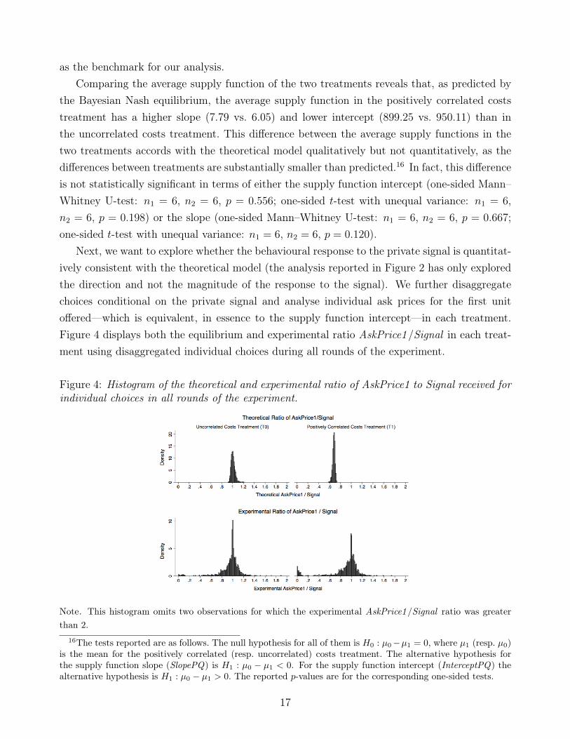
Next, we want to explore whether the behavioural response to the private signal is quantitat-ively consistent with the theoretical model (the analysis reported in Figure 2 has only exploredthe direction and not the magnitude of the response to the signal). We further disaggregatechoices conditional on the private signal and analyse individual ask prices for the first unitoffered—which is equivalent, in essence to the supply function intercept—in each treatment.Figure 4 displays both the equilibrium and experimental ratio AskPrice1/Signal in each treat-ment using disaggregated individual choices during all rounds of the experiment.

Figure 4: Histogram of the theoretical and experimental ratio of AskPrice1 to Signal received forindividual choices in all rounds of the experiment.

Note. This histogram omits two observations for which the experimental AskPrice1/Signal ratio was greaterthan 2.

16The tests reported are as follows. The null hypothesis for all of them is H0 : µ0−µ1 = 0, where µ1 (resp. µ0)is the mean for the positively correlated (resp. uncorrelated) costs treatment. The alternative hypothesis forthe supply function slope (SlopePQ) is H1 : µ0 − µ1 < 0. For the supply function intercept (InterceptPQ) thealternative hypothesis is H1 : µ0 − µ1 > 0. The reported p-values are for the corresponding one-sided tests.

17

In the uncorrelated costs treatment, the Bayesian Nash equilibrium predicts that the ratioof AskPrice1 to Signal is between 0.92 and 1.2, with both the mean and the median equalto 1.01. In other words, in this treatment the Bayesian Nash equilibrium predicts that AskPrice1will be (on average) equal to the signal received.17 Experimental choices in the uncorrelatedcosts treatment, as illustrated in the lower left graph of Figure 4, reveal that the mean of theAskPrice1/Signal ratio is similar to the mean (0.96) of its theoretical counterpart—but with alarger standard deviation owing to the heterogeneity in individual choices.

In the positively correlated costs treatment, the theoretically predicted AskPrice1/Signal

ratio is between 0.58 and 0.73, with both the mean and the median equal to 0.68; thus theequilibrium predicts that AskPrice1 will be lower than the signal received. The experimentaldistribution has a mean of 0.91 and median of 0.99, which means that: (i) for a given signal,AskPrice1 is (on average) larger than predicted by the Bayesian Nash equilibrium in this treat-ment; and (ii) subjects in the positively correlated costs treatment are strongly guided, whenchoosing AskPrice1, by the signal received (lower right graph of Figure 4) and so may choose anumber close to the signal received (since it acts as a focal point).

The foregoing analysis illustrates systematic divergences between behaviour—that is, howsubjects respond (through the supply function intercept) to the private signal—and BayesianNash equilibrium prediction in the positively correlated costs treatment. We interpret this resultas offering additional evidence that subjects, when setting the supply function intercept, do notaccount for the effects of correlation among costs and consequently respond too strongly to thesignal received.

The next result concerns the evaluation of Hypotheses (C) and (D).

Result 2 (Differences between experimental behaviour and theoretical predictions;differences in the average supply function between treatments). (i) The averagesupply function in the uncorrelated costs treatment is close to the correspondingequilibrium prediction; however, we reject the hypothesis that the average supplyfunction in the positively correlated costs treatment is the same as the correspond-ing equilibrium prediction. (ii) Differences in the average supply function betweentreatments are not statistically significant.

Thus we do not find empirical support for Hypothesis (C) or Hypothesis (D). In addition,Result 2 suggests that the generalised winner’s curse is a prevalent phenomenon in the positivelycorrelated costs treatment. The explanation is that: (a) behaviour in the uncorrelated coststreatment is consistent with the theoretical prediction and so can serve as a benchmark forsubjects that fall prey to the generalised winner’s curse; and (b) average behaviour in the

17The variables AskPrice1 and InterceptPQ are related as follows: AskPrice1 = InterceptPQ + SlopePQ .In each round, each subject was asked to specify (AskPrice1 ,AskPrice2 ); therefore, Ask Price1 more clearlyreflects how participants made their decisions.

18

positively correlated costs treatment is not different than average behaviour in the uncorrelatedcosts treatment.

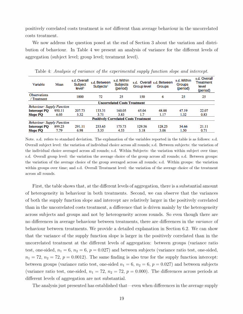
We now address the question posed at the end of Section 3 about the variation and distri-bution of behaviour. In Table 4 we present an analysis of variance for the different levels ofaggregation (subject level; group level; treatment level).

Table 4: Analysis of variance of the experimental supply function slope and intercept.

Note. s.d. refers to standard deviation. The explanation of the variables reported in the table is as follows: s.d.Overall subject level: the variation of individual choice across all rounds; s.d. Between subjects: the variation ofthe individual choice averaged across all rounds; s.d. Within Subjects: the variation within subject over time;s.d. Overall group level: the variation the average choice of the group across all rounds; s.d. Between groups:the variation of the average choice of the group averaged across all rounds; s.d. Within groups: the variationwithin groups over time; and s.d. Overall Treatment level: the variation of the average choice of the treatmentacross all rounds.

First, the table shows that, at the different levels of aggregation, there is a substantial amountof heterogeneity in behaviour in both treatments. Second, we can observe that the variancesof both the supply function slope and intercept are relatively larger in the positively correlatedthan in the uncorrelated costs treatment, a difference that is driven mainly by the heterogeneityacross subjects and groups and not by heterogeneity across rounds. So even though there areno differences in average behaviour between treatments, there are differences in the variance ofbehaviour between treatments. We provide a detailed explanation in Section 6.2. We can showthat the variance of the supply function slope is larger in the positively correlated than in theuncorrelated treatment at the different levels of aggregation: between groups (variance ratiotest, one-sided, n1 = 6, n2 = 6, p = 0.027) and between subjects (variance ratio test, one-sided,n1 = 72, n2 = 72, p = 0.0012). The same finding is also true for the supply function intercept:between groups (variance ratio test, one-sided n1 = 6, n2 = 6, p = 0.027) and between subjects(variance ratio test, one-sided, n1 = 72, n2 = 72, p = 0.000). The differences across periods atdifferent levels of aggregation are not substantial.

The analysis just presented has established that—even when differences in the average supply

19

function of each treatment are insignificant—the variance in the supply function slope andintercept is greater in the positively correlated than in the uncorrelated costs treatment.

Figure 5 plots the empirical cumulative distribution function (ECDF) for the supply functionslope and intercept in each treatment, where the source data for these graphs are the disaggreg-ated individual choices made by subjects during the first and last five rounds of bidding. Thesetwo time periods are important because they allow us to summarise behaviour at the beginningof the experiment, when subjects have no experience, and at the end of the experiment, whenthey have bid for 20 rounds.

Figure 5: Empirical cumulative distribution function (ECDF) for the supply function slope andintercept in the first five and last five rounds of bidding.

There is a significant difference between treatments as regards the ECDFs of supply functionslopes in both the first and last five rounds of bidding. The ECDF of supply function slopes inthe positively correlated costs treatment first order stochastically dominates the ECDF of slopesin the uncorrelated costs treatment both in the first and last five rounds (in a stronger way inthe latter). In fact, we can reject the hypothesis that the distribution of slopes is the samein the two treatments during the first five rounds of bidding (Kolmogorov–Smirnov equalityof distributions test: n1 = 360, n2 = 360, p = 0.023) and also during the last five rounds(Kolmogorov–Smirnov equality of distributions test: n1 = 360, n2 = 360, p = 0.000).18

18Repeating the same Kolmogorov–Smirnov equality of distributions test for the intermediate periods, ingroups of five rounds, we find that the distribution of slopes in the two treatments is significantly different in allintermediate time periods considered; this result is significant at the 5% level.

20

With regard to the supply function intercepts, we can see that the differences in ECDFsbetween treatments are quite small in the first five rounds of bidding, for which they are notstatistically significant (Kolmogorov–Smirnov equality of distributions test: n1 = 360, n2 = 360,p = 0.689). In the last five rounds of bidding, however, differences in the distribution ofsupply function intercepts are more substantial—albeit mainly driven by a few subjects, inthe positively correlated costs treatment, who bid a supply function with a very low intercept.Even so, we can reject the hypothesis that the ECDFs of supply function intercepts betweentreatments are the same in the last five rounds of bidding (Kolmogorov–Smirnov equality ofdistributions test: n1 = 360, n2 = 360, p = 0.009).19

We now address the question posed at the end of Section 3 about the variation and distri-bution of behaviour.

Result 3 (Difference in the distributions of the supply function slope and interceptbetween treatments). (i) There is a substantial amount of heterogeneity in beha-viour in both treatments. Variances in the supply function slope and intercept arerelatively greater in the positively correlated than in the uncorrelated costs treat-ment because of the heterogeneity in subjects’ and groups’ behaviour, not becauseof heterogeneity across rounds. (ii) Using individual choices, we reject the hypo-thesis that the distribution of supply function slopes is the same in both treatmentsfor the first five and last five rounds of bidding. The cumulative distribution func-tion of supply function slopes in the positively correlated costs treatment first orderstochastically dominates the cumulative distribution function of slopes in the uncor-related costs treatment both in the first and last five rounds. We cannot reject thehypothesis that the distribution of supply function intercepts is the same in bothtreatments for the first five rounds of bidding, but we do reject the hypothesis thatthe distribution of supply function intercepts is the same in both treatments for thelast five rounds of bidding.

Result 3 indicates that there are differences in the distribution of supply functions betweentreatments. The differences in behaviour between treatments are consistent with the directionpredicted by the theoretical model. We shall examine this issue more closely in Section 6.2.

In sum, the results reported in this section have shown that average differences in behaviourbetween treatments are not statistically significant. However, there are significant differences inthe distribution of supply functions between treatments, suggesting that that some subjects inthe positively correlated costs treatment—because they ignore the correlation among costs and

19Repeating the same Kolmogorov–Smirnov equality of distributions test for the intermediate periods, ingroups of five rounds, we find that the distribution of intercepts in the two treatments is not significantly differentin the second and third groups of five rounds (Rounds [6, 10] and Rounds [11, 15]) but that the distributionbecomes significantly different after the 15th round.

21

its adverse effects—fall prey to the generalised winner’s curse while others do not.20 The moredetailed examination in Section 6 seeks to determine whether these results are driven by a smallproportion of subjects or whether the generalised winner’s curse is prevalent in the positivelycorrelated costs treatment.

5.2 Analysis of experimental outcomes (market price and profits) and

efficiency of allocations

Table 5 reports experimental outcomes and the corresponding predictions in terms of the marketprice, profits, and efficiency levels of the allocations (as captured by deadweight losses) togetherwith the corresponding theoretical predictions.21 Our unit of analysis is the group average,which aggregates outcomes within the group and across rounds.22

Table 5: Average outcomes, and their corresponding theoretical predictions, by treatment.

Note. The theoretical predictions for outcomes and efficiency refer to ex ante expected market prices, ex anteexpected profits, and ex ante expected deadweight loss at the equilibrium allocation.The standard deviation (s.d.) is given in parentheses below the reported average. For profits reported standarddeviations are at the individual level; for market price and deadweight loss, standard deviations are at the marketlevel.

Turning now to average market prices, we see that the difference in these prices betweentreatments is not statistically significant (one-sided Mann–Whitney U-test: n1 = 6, n2 = 6,p = 0.556; one-sided t-test with unequal variance: n1 = 6, n2 = 6, p = 0.210). In bothtreatments, average market prices are lower than theoretically predicted: 92.7% and 72.6% ofthe theoretically predicted values in the uncorrelated and positively correlated costs treatment,respectively.

20Refer to Section 3 for an explanation of the generalised winner’s curse.21See Appendix A for the formulae which have been used to calculate the outcome and efficiency variables.22The tests reported for the rest of the section are as follows. The null hypothesis for all of them is H0 :

µ0 − µ1 = 0, where µ1 (resp. µ0) is the mean for the positively correlated (resp. uncorrelated) costs treatment.The alternative hypothesis for market price and profits is H1 : µ0−µ1 < 0. For deadweight loss, the alternativehypothesis is H1 : µ0 − µ1 > 0. The reported p-values are for the corresponding one-sided tests.

22

Average profits in each treatment are substantially lower than their corresponding ex anteequilibrium predictions. In particular, average profits are 40.2% (resp., 11.7%) of the theoret-ically predicted values in the uncorrelated (resp., positively correlated) costs treatment.23 Wealso observe that, in the correlated costs treatment, bidders forgo a large percentage of ex anteexpected profits—as typically occurs in auctions where bidders ignore the correlation amongcosts (Kagel and Levin 1986). The average difference in profits between the two treatmentsis not statistically significant (one-sided Mann–Whitney U-test: n1 = 6, n2 = 6, p = 0.389;one-sided t-test with unequal variance: n1 = 6, n2 = 6, p = 0.716).

In order to further understand the very large divergence between theoretical and experi-mental profits, we decompose this difference into the various components of profits (revenues,production costs and transaction costs) and we illustrate it by a waterfall chart in Figure 6.

Figure 6: Decomposition of the differences between theoretical and experimental profits into thevarious components in each treatment.

Note. In each graph, the first bar of each graph corresponds to ex-ante expected profits at the equilibriumallocation. The second bar to the difference between theoretical and experimental revenues; the third bar tothe difference between theoretical and experimental production costs; The fourth bar to the difference betweentheoretical and experimental transaction costs. The last bar corresponds to average experimental profits. Awaterfall chart shows how an initial value (whole column) increases or decreases by a sequence of intermediatepositive or negative values (floating columns) to reach a final value (whole column). A colour-code is used fordistinguishing positive (grey) from negative (black) intermediate values.

The figure shows that, in both treatments, the largest difference between theoretical and ex-perimental profits is driven by the revenues component.24 Therefore, differences in experimental

23The theoretical predictions assume that all subjects play the Bayesian Nash equilibrium in the correspondingtreatment. Note that if one subject realises that her opponents are not playing the Bayesian Nash equilibriumthen it is not optimal for her to play the Bayesian Nash equilibrium, either; therefore, ex ante expected profitsare different. See Section 6 for further discussion.

24Recall that profits of seller i at time t are πit = ptxit− θitxit− λ2x

2it. The first term corresponds to revenues;

the second to production costs and the third to transaction costs.

23

and theoretical profits are primarily driven by market prices being lower than theoretically pre-dicted, since the supply functions submitted by subjects are flatter than the equilibrium supplyfunction and exhibit a large heterogeneity in both treatments; the difference and heterogeneityhere are more pronounced in the positively correlated costs treatment, as seen in Table 3. Thesedifferences in market prices are amplified when translated to revenues since the market price ismultiplied by units sold, the average of which is 33.33.25

With regard to the efficiency of experimental allocations, there is a difference betweentreatments—in the direction predicted by Hypothesis (F)—but it is not statistically signific-ant (one-sided Mann–Whitney U-test: n1 = 6, n2 = 6, p = 0.583; one-sided t-test with unequalvariance: n1 = 6, n2 = 6, p = 0.242). So that we can better understand why the more het-erogeneous behaviour in the positively correlated (than in the uncorrelated) costs treatmentdoes not lead to differences in the efficiency of allocations, we decompose the experimentaldeadweight loss (dwl) into three components as follows:

dwl = (λ

2)(

n∑i=1

(xei −q

n)2 + (xoi −

q

n)2 − 2(xei −

q

n)(xoi −

q

n)), (3)

The first term of (3) captures the variance of the experimental allocation, the second termcaptures the variance of the efficient allocation, and the third term captures the covariance ofthe experimental and efficient allocations.

After comparing these three components of deadweight loss across treatments, we can makeseveral observations. First, variances in the experimental allocations do not differ betweentreatments. Second, the variance in efficient allocations is greater in the uncorrelated than inthe positively correlated costs treatment; this finding corresponds to the theoretical predictionthat follows from the experiment’s configuration of parameters. Third, the covariance of theexperimental and efficient allocations is substantially larger in the uncorrelated than in thepositively correlated costs treatment. When we consider both the three dwl components andtheir corresponding coefficients, we find that the difference between treatments with regard tovariance in the efficient allocations is offset by the difference in the covariance term. For a graphdisplaying of these components, see Figure 10 (and Table 14) in Appendix F.

We also compare the deadweight losses of the experimental and equilibrium allocations. Thevalues reported in Table 5 show that, in both treatments, the average experimental deadweightlosses are considerably larger than those of the equilibrium allocations. This result is explainedas follows. In both treatments, the deadweight losses at the equilibrium allocations are due toinsufficient dispersion and covariation with respect to the corresponding efficient allocations. In

25Our analysis of the variance in experimental outcomes (see Appendix F) establishes that variances in marketprice, profits, and deadweight loss are driven by neither subject nor group heterogeneity but rather, for the mostpart, by heterogeneity across rounds.

24

the uncorrelated costs treatment, the deadweight loss at the experimental allocation is largerthan at the equilibrium because the covariation between the experimental and efficient alloca-tions is not enough to compensate for the sum of the variances in the experimental and efficientallocations (these two variances are very similar). In the positively correlated costs treatment,however, the difference between the deadweight losses of the experimental and equilibrium al-locations is driven mainly by the former’s comparatively greater variance.

We now evaluate Hypotheses (E) and (F), which address differences in experimental out-comes between treatments.

Result 4 (Differences in average market prices, profits, and deadweight lossesbetween treatments). There is no average difference between treatments with respectto market prices, profits, or deadweight losses.

Result 4 implies that market power is not greater in the positively correlated than in theuncorrelated costs treatment. Hence we find no supporting evidence for Hypothesis (E) orHypothesis (F).

5.3 Time trends in behaviour and outcomes

Figure 7 plots, for each treatment, the evolution across rounds of the supply function interceptand slope as well as the corresponding theoretical predictions.

Figure 7: Evolution across rounds of the supply function slope and intercept in each treatment.

Note. The theoretical supply function intercept is calculated using the average signal received in each roundfor each treatment; the theoretical predictions are calculated using the actual draws of the signal received. SeeAppendix B for a comparison between actual draws and the theoretical distribution. SF = supply function;T0 = uncorrelated costs treatment; T1 = positively correlated costs treatment.

25

The left-hand side of this figure shows that the supply function intercept increases acrossrounds in the uncorrelated costs treatment (a regression of the supply function intercept onround yields a coefficient of 2.28, with p = 0.002); in the positively correlated costs treatment,the intercept increases during the first ten rounds of play and then decreases across rounds(a regression of the supply function intercept on round yields an insignificant coefficient withp = 0.927). The right-hand side of Figure 7 shows that the average supply function slopebecomes smaller across rounds in the uncorrelated costs treatment (a linear regression of thesupply slope on round yields a coefficient of −0.096 with p = 0.000), but there is no significanttime trend in the positively correlated costs treatment (a linear regression of supply functionslope on round yields an insignificant coefficient with p = 0.212).26 Thus we find that theevolution of behaviour across rounds is different in each treatment.

Furthermore, we observe that the change in behaviour (with regard to both the intercept andslope of the supply function) is more pronounced in the first ten rounds of play and especially inthe first five rounds. In the last five rounds of play, the average supply function slope is stable;however, during these rounds the supply function intercept increases sharply (resp., decreases)in the uncorrelated (resp., positively correlated) costs treatment.

In the uncorrelated costs treatment, we find that both the intercept and slope of the sup-ply function tend toward the theoretical prediction as the number of rounds increases. Yet inthe positively correlated costs treatment we observe no decline across rounds in the differencebetween the average supply function and the theoretical prediction, which indicates that naïvebehaviour persists.

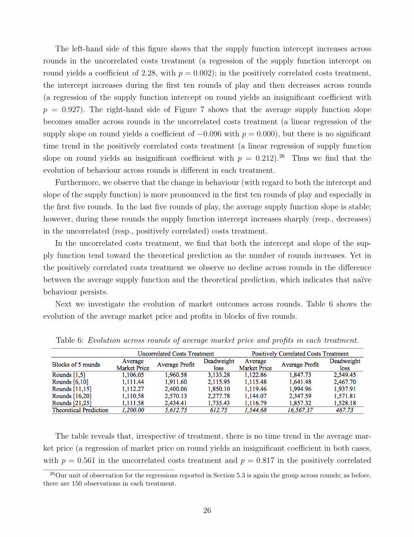
Next we investigate the evolution of market outcomes across rounds. Table 6 shows theevolution of the average market price and profits in blocks of five rounds.

Table 6: Evolution across rounds of average market price and profits in each treatment.

The table reveals that, irrespective of treatment, there is no time trend in the average mar-ket price (a regression of market price on round yields an insignificant coefficient in both cases,with p = 0.561 in the uncorrelated costs treatment and p = 0.817 in the positively correlated

26Our unit of observation for the regressions reported in Section 5.3 is again the group across rounds; as before,there are 150 observations in each treatment.

26

costs treatment). In addition, we find that profits increase after the tenth round in the uncor-related costs treatment but not in the positively correlated costs treatment (regressing profitson round yields an insignificant coefficient, with p = 0.103 in the uncorrelated costs treat-ment and p = 0.577 in the positively correlated costs treatment).27 Deadweight losses decreaseover time in both treatments (a regression of deadweight loss on round gives a coefficient of−56.40 with p = 0.003 in the uncorrelated costs treatment and of −56.29 with p = 0.000 in thepositively correlated costs treatment). In the uncorrelated costs treatment, deadweight lossesare decreasing in the number of rounds because the covariance between the experimental andefficient allocations increases substantially. In the positively correlated costs treatment, dead-weight losses decrease for a different reason: variance in the experimental allocations decreasessignificantly with the number of rounds, thus reducing the difference between the variance ofthe experimental and efficient allocations.

Finally, we report an additional finding about the evolution of behaviour across rounds. Thisresult emerged from our analysis of the experimental data.

Result 5 (Evolution of supply functions and outcomes across rounds). (i) Theevolution of supply functions across rounds is different in the two treatments: inthe uncorrelated costs treatment, average behaviour starts close to the equilibriumprediction and, across rounds, moves even closer to that prediction; in the positivelycorrelated costs treatment, average behaviour starts far from from the equilibriumprediction and, across rounds, does not move much closer to that prediction. (ii) Inboth treatments, deadweight losses decrease as subjects gain bidding experience;however, we find no evidence that market prices evolve across rounds. In the uncor-related costs treatment, there is some evidence that profits increase as subjects gainbidding experience. In the positively correlated costs treatment, we do not find thatprofits evolve across rounds.

Result 5 suggests that the learning process may be different in the two treatments, a possibilitythat we explore further in Section 6.3. The finding that, as the number of rounds increases, beha-viour in the positively correlated costs treatment does not move much closer to the equilibriumprediction suggests that naïve behaviour persists in this treatment.

27Although we observe a time trend in profits (after the tenth round) in the uncorrelated costs treatment,that trend is not statistically significant when data are aggregated at the group level. However, in Section 5.4we establish that this time trend is statistically significant when choices are considered at the individual levelacross rounds.

27

6 Examining the Data More Closely

In this section, we first study a subjects’ strategic incentives; we then perform cluster analysisto descriptively study how close subjects’ choices are to the various theoretical benchmarks.Third, we provide a description of the determinants of the evolution of behaviour across rounds,and finally we analyse subjects’ responses to our post-experiment questionnaire. Overall, allthe parts provide an explanation of the results we observe.

6.1 Best-response analysis

Bidding in the positively correlated costs treatment involves a higher degree of strategic com-plexity than bidding in the uncorrelated costs treatment. This is because the market price isnot informative about costs in the uncorrelated costs treatment whereas, in the positively cor-related costs treatment, equilibrium reasoning requires that a subject correctly understand howthe market price is informative about the average cost, which also involves having the correcthigher-order beliefs. To increase our understanding of a bidder’s strategic incentives, we derivetheoretically the best-response strategy of seller i while assuming that she knows the averagestrategy of rivals, which determines her residual demand. We then compute the comparativestatics of the best-response with respect to the average strategy of those rivals.

In each treatment, we first analyse the best-response supply function to the rivals’ averagestrategy during the first five rounds of bidding.28 In the uncorrelated costs treatment, theaverage supply function for the first five rounds is steeper and has a lower intercept than theequilibrium. If we assume that rivals bid as the “representative seller” during the first fiverounds, then seller i’s best-response is to bid a supply function that is flatter and has a higherintercept than that of her rivals but that is still steeper (and with a higher intercept) than theequilibrium supply function. In the positively correlated costs treatment, however, the averagesupply function for the first five rounds deviates substantially from the equilibrium supplyfunction: the former is much flatter and has a higher intercept than predicted. In this case,seller i’s best-response supply function is steeper than that of her rivals’ yet flatter than theequilibrium supply function. The intercept of seller i’s best-reply supply function is also betweenthese two benchmarks. We illustrate these features of the best-response supply function in eachtreatment and compare them with the corresponding equilibrium supply functions in Figure 8.

28Since behaviour does not evolve much across rounds, it follows that the features of the best-response supplyfunction would be similar had we considered alternative definitions of the rivals’ average strategy.

28

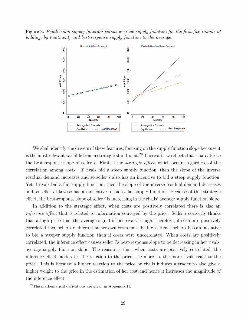
Figure 8: Equilibrium supply function versus average supply function for the first five rounds ofbidding, by treatment, and best-response supply function to the average.

We shall identify the drivers of these features, focusing on the supply function slope because itis the most relevant variable from a strategic standpoint.29 There are two effects that characterisethe best-response slope of seller i. First is the strategic effect, which occurs regardless of thecorrelation among costs. If rivals bid a steep supply function, then the slope of the inverseresidual demand increases and so seller i also has an incentive to bid a steep supply function.Yet if rivals bid a flat supply function, then the slope of the inverse residual demand decreasesand so seller i likewise has an incentive to bid a flat supply function. Because of this strategiceffect, the best-response slope of seller i is increasing in the rivals’ average supply function slope.

In addition to the strategic effect, when costs are positively correlated there is also aninference effect that is related to information conveyed by the price. Seller i correctly thinksthat a high price that the average signal of her rivals is high; therefore, if costs are positivelycorrelated then seller i deduces that her own costs must be high. Hence seller i has an incentiveto bid a steeper supply function than if costs were uncorrelated. When costs are positivelycorrelated, the inference effect causes seller i’s best-response slope to be decreasing in her rivals’average supply function slope. The reason is that, when costs are positively correlated, theinference effect moderates the reaction to the price, the more so, the more rivals react to theprice. This is because a higher reaction to the price by rivals induces a trader to also give ahigher weight to the price in the estimation of her cost and hence it increases the magnitude ofthe inference effect.

29The mathematical derivations are given in Appendix H.

29

Suppose seller i bids in the positively correlated costs treatment and that seller i’s rivals fallprey to the generalised winner’s curse, thus bidding as in the equilibrium of the uncorrelatedcosts treatment. Then the slope of seller i’s best-response supply function is increasing in thesupply function slope of rivals, which means that the strategic effect dominates the inferenceeffect. However, the inference effect does moderate the magnitude of the increase in the best-response supply function’s slope as a result of an increase in the slope of her rivals’ supplyfunction—when costs are uncorrelated. It follows that the optimal response for seller i is to bida supply function whose slope is between the slope of naïve sellers’ (average) supply functionand the slope of the equilibrium supply function. In other words: a sophisticated seller whois best responding to naïve rivals has an incentive to bid a flatter supply function than theequilibrium would predict, which leads to the behaviour of naïve and sophisticated sellers beingless distinct. An equivalent result was first noted by Camerer and Fehr (2006) in the contextof games characterised by strategic complementarities and by sophisticated and boundedlyrational subjects.30 Figure 11 (in Appendix H) plots, for each treatment, the best-responsesupply function slope as a function of rivals’ average supply function slope.

In sum, the positively correlated costs treatment presents a higher degree of strategic com-plexity than the uncorrelated costs treatment. This explains why average choices in the posit-ively correlated costs treatment are farther from the equilibrium than in the uncorrelated coststreatment. In the former, the best-response strategy of a sophisticated seller who best respondsto her rivals’ actual choices is one that falls between the equilibrium of the positively correlatedcosts treatment and the benchmark of the generalised winner’s curse (i.e., the equilibrium ofthe uncorrelated costs treatment). Therefore, we see less difference in behaviour—between treat-ments and types of subjects (naïve and sophisticated)—than is predicted by the equilibrium.

6.2 Cluster analysis

We can use cluster analysis to conduct a descriptive study of experimental choices; this approachenables us to “organise” the heterogeneity in behaviour and relate it to the various theoreticalbenchmarks. We shall present the results of analysing subjects’ choices in the first five rounds ofbidding, when strategic thinking is most relevant, and also in the last five rounds, when subjectsare most experienced.

We use a model-based clustering technique, which is based on mixture models, for endo-genously and simultaneously determining (a) the number of clusters and (b) the type of modelcharacterised by properties of the underlying probability distributions (orientation, volume, and

30We can also relate best-response and equilibrium strategies to models of strategic thinking. In the termino-logy of a level-k model (Nagel 1995), a level-1 subject would best respond to the strategies of rivals believing thatrivals are level-0 subjects (e.g., subjects who fall prey to the generalised winner’s curse). So for k ≥ 1, a level-ksubject would best respond to rivals believing they are all of level k − 1. The Bayesian Nash equilibrium wouldthen be obtained as the limiting behaviour when all subjects perform an infinite number of level-k iterations.

30

shape). The Bayesian information criterion (BIC) allows us to select the most appropriate clus-tering model. We implement this procedure using the Mclust package in R (developed by Fraleyand Raftery 2002), which uses the expectation-maximisation (EM) algorithm.

The data used for the cluster analysis are as follows. We first compute the average subjectchoice for each group of five rounds. Each choice is two-dimensional in that they each consistof the supply function slope and intercept. We then compute the deviation of each individual’saverage choice with respect to the corresponding equilibrium benchmark, and the resultingdeviations form the basis of our cluster analysis. We conduct the cluster analysis separatelyfor each treatment and each group of five rounds. To facilitate comparisons within a giventreatment—and our interpretation thereof—we choose the same number of clusters and type ofmodel in each group of five rounds.31

Table 7 summarises the results of our cluster analysis by reporting the type of model, thenumber of components, the frequency of subjects in each cluster, and the average supply slopeand intercept of subjects belonging to a particular cluster (in Appendix I we provide resultsfrom cluster analysis based on the intermediate time periods in five-round blocks). The findingsreported in Table 7 are plotted in Figure 9.

In the uncorrelated costs treatment, the BIC yields two clusters with a model of VEV(varying volume, equal shape, and varying orientation with ellipsoidal distribution) type. Inboth time periods, cluster 1 groups subjects whose choices are close to both the Bayesian Nashequilibrium choice and the best-response to the average choice. Cluster 1 contains 58% of thesubjects in the first five rounds, and this percentage rises to 72% in the last five rounds. Subjectsin cluster 2 bid a steeper supply function with a lower intercept than the equilibrium prediction.These results suggest that most subjects’ behaviour in the uncorrelated costs treatment accordsfairly well with the theoretical predictions (as already indicated by the average results reportedin Section 5). Furthermore, we observe that 14% of the subjects move from cluster 2 to cluster1 from the beginning to the end of the experiment.

31In the uncorrelated costs treatment, the five clustering models presented in the text (and in Appendix I) havethe highest possible BIC or there is a BIC difference of less than 2 with respect to the optimal model. (Fraleyand Raftery 2002 argue that, if the difference in BIC between two models is less than 2, then this constitutesat least weak evidence that one model is better than the other.) In the positively correlated costs treatment,no single model has the highest BIC for all five sets of data. Hence we consider the second-best model for allfive time periods, which is a three-component model of VEI (varying volume, equal shape, and coordinate axesorientation with diagonal distribution) type.

31

Table 7: Descriptive statistics characterising each cluster.

Note. The intercept of the equilibrium supply function is calculated using the average signal realisation. Standarddeviations (s.d.) are reported in parentheses.

In the positively correlated costs treatment, the BIC yields three clusters and a model ofVEI type (see note 30). In the first five rounds, no subject bids as in the equilibrium. In theserounds, we see that: 58% of the subjects are in cluster 3, which approximately corresponds to thebenchmark of the generalised winner’s curse (equilibrium of the uncorrelated costs treatment);36% of the subjects are in cluster 2, which means their behaviour is not inconsistent with thatof a sophisticated bidder (i.e., they bid a supply function close to the average theoretical bestreply); and 6% of the subjects are in cluster 1, meaning that they choose a supply function withan extremely steep slope and a very low intercept (close to zero). The subjects in cluster 1 areattracted to the zero-intercept focal point.32

32These cluster results can be loosely related to the level-k model of strategic thinking. Subjects in cluster 3can be thought to be level-0; subjects in cluster 2 to be level-1; and subjects in cluster 1 cannot be easily relatedto a level of strategic thinking since one dimension (the supply function slope) is close to the equilibrium butthe other dimension (the supply function intercept) is far from all benchmarks.

32

Figure 9: Results of cluster analysis.

Note. Each data point corresponds to a subject’s two-dimensional (slope and intercept) average choice over thefirst five or last five rounds of bidding. The x-axes (resp.,y-axes) represent the difference between theoreticaland experimental supply function slopes (resp., intercepts). The black dashed lines plot the equilibrium supplyfunction slope and intercept in each treatment, where (0, 0) corresponds to the equilibrium. In the two graphscorresponding to the positively correlated treatment, there are green dashed lines that plot the generalisedwinner’s curse benchmark (i.e., the equilibrium of the uncorrelated costs treatment).

To explore further the relationship between clusters and optimal behaviour, in Table 18 ofAppendix I we summarise—for each cluster—the average difference between the experimentalsupply function and the theoretical best-response supply function. In the uncorrelated coststreatment, cluster 1 groups subjects whose supply functions are close to the theoretical best-response in both time periods; in the positively correlated costs treatment, cluster 2 groupssubjects whose choices are close to the theoretical best-response slope and intercept in bothtime periods. In the positively correlated costs treatment, subjects in cluster 1 bid supplyfunctions that are too steep and have too low an intercept vis-à-vis the theoretical best replywhile subjects in cluster 3 bid supply functions that are too flat and have too high an intercept.

In the positively correlated costs treatment, there is an exodus of subjects from cluster 3to cluster 2 as the experiment progresses from the first five to the last five rounds of bidding;that movement might lead us to infer that most subjects bid a supply function with a steeperslope. However, Table 7 shows that the average supply function slope of subjects in clusters2 and 3 actually decreases from the first five to the last five rounds of bidding, which meansthat—during those last five rounds—the benchmark of the generalised winner’s curse is locatedbetween clusters 2 and 3. In light of this evidence, we conclude that there are no importantchanges in the evolution of clusters between the beginning and the end of the experiment. Wecan summarise these findings as follows.

Result 6 (Cluster analysis). (i) In the uncorrelated costs treatment, 58% of thesubjects are in the same cluster as the equilibrium in the first five rounds—a percent-age that increases to 72% in the last five rounds. This cluster groups subjects whosesupply function is closest to the theoretical best-response. (ii) In the positivelycorrelated costs treatment, no subject bids as predicted by the equilibrium in eitherthe first five rounds or the last five rounds of bidding. The proportion of subjectswho are in the same cluster as the “generalised winner’s curse” benchmark is 58%in the first five rounds of bidding and 50% in the last five rounds; the proportion ofsubjects whose bidding behaviour is not inconsistent with sophisticated behaviour(i.e., best responding to the average supply function) is 36% in the first five roundsand 42% in the last five rounds of bidding; and the proportion of subjects who bida steep supply function with a low intercept is 6% (resp. 8%) in the first (resp. last)five rounds of bidding.

Observe that, for a subject who is best responding to actual choices in the positively correlatedcosts treatment, it is individually optimal to bid a supply function with a flatter slope and witha higher intercept than the equilibrium would predict. This fact explains why average behaviourand outcomes are not sufficiently differentiated between treatments and hence why it is difficultempirically to distinguish the behaviour of naïve and sophisticated subjects. Furthermore, if

34

some subjects never learn (or learn very slowly) and remain in cluster 3, then a subject whois best responding to actual choices may have no incentive to bid increasingly steeper supplyfunctions during the course of the experiment. This may explain why slopes do not evolve towardthe equilibrium prediction in the positively correlated costs treatment. The rest of Section 6is dedicated to uncovering what determines the evolution of choices across rounds in the twotreatments. Section 6.3 conducts a more detailed analysis of behaviour since it considers theeach individual choice across all rounds of the experiment (rather than in blocks of 5 periods ashas been done in this section).

6.3 Evolution of choices across rounds

Our goal is to provide a description of the evolution behaviour observed experimentally andthereby to understand what drives differences in the changes of behaviour (across rounds) inthe two treatments. The experimental design provided subjects with complete feedback aftereach round, feedback that included each subjects’ own choice and profits as well as the choicesand profits of the other two market participants. Subjects might be therefore be influenced bythe average choices of rivals in the same group. We designed this high-information environment,and stipulated 25 rounds per session, so as to foster participants’ learning about the equilibrium.A subject’s use of a particular learning model depends on both the available information andher cognitive abilities. Given the experiment’s complexity, we considered only those learningmodels in which subjects had the necessary information to learn.

We therefore consider that the evolution of behaviour across rounds can be explained interms of three main categories of learning models (for an excellent review, see Camerer 2003):experiential learning, in which subjects learn from their own experience; imitation-based learn-ing, in which subjects choose—after the first round—a strategy chosen by other players inthe previous round; and belief learning, an adaptive style whereby subjects update their be-liefs based on the history of play. Unlike the case of Cournot competition, there are very fewtheoretical results on the convergence properties of learning models in the context of supplyfunction competition with private information.33 In this section, then, we aim only to providean informative description of actual behaviour across rounds.

Our empirical strategy follows the approach of Huck et al. (1999) and Bigoni and Fort(2013); more specifically, we consider a representative model (or models) from each of the threecategories just described. Moreover, we presume that the supply function slope is the strategicvariable best able to summarise how a subject adjusts her behaviour across rounds. We forgoanalysing the dynamics of the supply function intercept because, in our view, the subjects donot have enough information to learn from it; that is, we provided no feedback on the signals

33For some general considerations, see Vives (2008, Chapter 7).

35

received by rivals. As a result, the supply function intercept could be affected by confoundingfactors, such as how subjects respond to the private signal. Note also that supply functionintercepts are nearly identical in the two treatments.

The type of experiential learning on which we focus is reinforcement learning (RL), wherebya player increases her probability of playing a strategy (i.e., the strategy is reinforced) as afunction of the profits previously earned via that strategy. A strategy’s “propensity” is thecumulative sum of the previous profits that it generated with such strategy, and a strategy’s“relative propensity” is its propensity divided by the aggregate propensities of all strategiesemployed in a given round (cf. Erev and Roth 1998). Our implementation of reinforcementlearning assumes that a player bids the supply function slope exhibiting the highest relativepropensity.

We then consider two models based on learning by imitation. Of these, the first is a payoff-independent model—imitation of the average (IA)—under which subjects imitate their rivals’average strategy in the previous round. The second is a payoff-dependent model, imitation ofthe best (IB), whereby subjects imitate the strategy of the subject who garnered the highestprofits in the previous round (and where that most successful player imitates herself).34

As a representative of belief learning models we consider best-response dynamics (BR),whereby subjects best respond to their rivals’ previous-round strategies.35 Recall that thefeatures of a best-response strategy were described, for each treatment, in Section 6.1.36

We estimate a dynamic panel regression to identify the determinants of each subject’s supplyfunction slope across rounds with respect to the various learning models described previously.37

Thus, we estimate the following equation:

SlopePQ it = γSlopePQ it−1 + βRLRLit−1 + βIAIAit−1

+ βIBIBit−1 + βBRBRit−1 + νi + ωit. (4)

Here SlopePQ it issubject i’s supply function slope in round t; SlopePQ it−1 is the supply function

34We have not considered learning models such as imitate the exemplary firm (Offerman et al. 2002), sincethis would require subjects to calculate the joint maximisation of profits for three “firms” producing a givenlevel of output. That task is far from trivial in our experimental environment of supply functions and privateinformation.

35The difference between the best-response analysis in this section and the version analysed elsewhere (inSection 6.1, Section 6.2, Appendix H, and Appendix I) is that here we consider the best-response to rivals’strategy of the previous rather than the current round.

36We do not consider the fictitious play model because it is cognitively more demanding than best-responsedynamics. In particular, it requires subjects to remember the average strategies of all previous rounds of play;best-response dynamics, in contrast, requires subjects to remember the strategies only of the other two playersin the previous round.

37As compared with Huck et al. (1999) we have added the reinforcement learning term. As compared withBigoni and Fort (2013), we have replaced the “trial and error” experiential learning model with the reinforcementlearning model, which has gained wider acceptance in the literature.

36

slope of subject i in the previous round (i.e., round t−1), which gives an indication of behaviouralpersistence; RLit−1 is the supply function slope corresponding to the highest relative propensitybased on player i’s profits in round t− 1 (reinforcement learning); IAit−1 is the average supplyfunction slope of i’s rivals in the previous round (imitation of the average); IBit−1 is the supplyfunction slope that corresponds to the highest profits of i’s rivals in round t−1 and if i’s profitswere the highest in period t − 1 then subject i imitates herself (imitation of the best); BRit−1

is subject i’stheoretical best reply to her rivals’ supply function slope in the previous round(best-response dynamics); ωit is the error term; and vi represents panel-level random effects.38

If a given learning model fully explained how a subject adjusts her supply function slopeacross rounds, then its regression coefficient would be 1 and the other coefficients would beinsignificant. In the more likely event that the model’s explanation is only partial, we expectits coefficient to be positive and significantly different from 0.

Table 8 presents the results from estimating equation (4)—for individual choices acrossrounds in each treatment—using the approach proposed by Arellano and Bover (1995) andBlundell and Bond (1998).39

Table 8: Dynamic panel estimation: Evolution of behaviour across rounds.

Note. Robust standard errors are given in parentheses.*, **, and *** denote significance at (respectively) the 10%, 5%, and 1% levels.

Columns [1] and [2] of Table 8 present the results of estimating equation (4) for the un-38Details of how these learning variables have been created are available from the authors upon request.39The estimation was conducted via Stata’s xtdpdsys command using the two-step estimator. The regressors

corresponding to each of the learning models were considered to be predetermined because, although possiblycorrelated to past errors, they are not correlated with future errors. The two restrictions on these instrumentsare that (i) we use at most one lag of the dependent variable as an instrument and (ii) each regressor appearsas contemporaneous and at most one lag is used as an instrument.In all the equations presented, the post-estimation specification test for autocorrelation of the error terms gives

no evidence of autocorrelation of order higher than 1 at the 10% significance level. In addition, we cannot rejectthe null hypothesis that the overidentifying restrictions are valid (Sargan test) for all the regressions displayed.

37

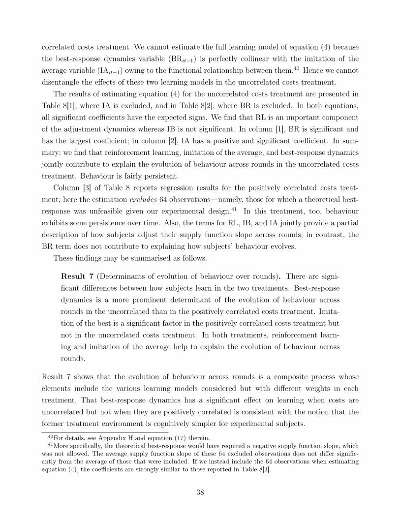
correlated costs treatment. We cannot estimate the full learning model of equation (4) becausethe best-response dynamics variable (BRit−1) is perfectly collinear with the imitation of theaverage variable (IAit−1) owing to the functional relationship between them.40 Hence we cannotdisentangle the effects of these two learning models in the uncorrelated costs treatment.

The results of estimating equation (4) for the uncorrelated costs treatment are presented inTable 8[1], where IA is excluded, and in Table 8[2], where BR is excluded. In both equations,all significant coefficients have the expected signs. We find that RL is an important componentof the adjustment dynamics whereas IB is not significant. In column [1], BR is significant andhas the largest coefficient; in column [2], IA has a positive and significant coefficient. In sum-mary: we find that reinforcement learning, imitation of the average, and best-response dynamicsjointly contribute to explain the evolution of behaviour across rounds in the uncorrelated coststreatment. Behaviour is fairly persistent.

Column [3] of Table 8 reports regression results for the positively correlated costs treat-ment; here the estimation excludes 64 observations—namely, those for which a theoretical best-response was unfeasible given our experimental design.41 In this treatment, too, behaviourexhibits some persistence over time. Also, the terms for RL, IB, and IA jointly provide a partialdescription of how subjects adjust their supply function slope across rounds; in contrast, theBR term does not contribute to explaining how subjects’ behaviour evolves.

These findings may be summarised as follows.

Result 7 (Determinants of evolution of behaviour over rounds). There are signi-ficant differences between how subjects learn in the two treatments. Best-responsedynamics is a more prominent determinant of the evolution of behaviour acrossrounds in the uncorrelated than in the positively correlated costs treatment. Imita-tion of the best is a significant factor in the positively correlated costs treatment butnot in the uncorrelated costs treatment. In both treatments, reinforcement learn-ing and imitation of the average help to explain the evolution of behaviour acrossrounds.

Result 7 shows that the evolution of behaviour across rounds is a composite process whoseelements include the various learning models considered but with different weights in eachtreatment. That best-response dynamics has a significant effect on learning when costs areuncorrelated but not when they are positively correlated is consistent with the notion that theformer treatment environment is cognitively simpler for experimental subjects.

40For details, see Appendix H and equation (17) therein.41More specifically, the theoretical best-response would have required a negative supply function slope, which

was not allowed. The average supply function slope of these 64 excluded observations does not differ signific-antly from the average of those that were included. If we instead include the 64 observations when estimatingequation (4), the coefficients are strongly similar to those reported in Table 8[3].

38

Notice that this result may appear to contrast with Result 6 which shows that, in thepositively correlated costs treatment, the proportion of subjects whose bidding behaviour is notinconsistent with sophisticated behaviour (i.e., best responding to the average supply function)is 36% in the first five rounds and 42% in the last five rounds of bidding. However, the analysisof Section 6.2 used the average subject choice for each group of five rounds while the dynamicanalysis of this section considers the individual choice for each round. Therefore, we concludethat on a round-to-round basis, subjects in the positively correlated costs treatment do notappear to be best responding to the choices of rivals in the previous round. However, thereis evidence that when aggregating rounds in groups of five, some subjects in the positivelycorrelated costs treatment (36% in the first five rounds and 42% in the last five rounds ofbidding) are close to the average best-response.

6.4 Post-experiment questionnaire: Analysis

Our experiment’s main result is that most subjects in the positively correlated treatment behaveas if they did not understand that the market price is informative about costs. Analysing theresponses given by subjects in our post-experiment questionnaire offers further evidence of thisinterpretation. We asked two questions: “Do you think that a high market price generally meansgood, mixed, or bad news about the level of your costs?” and then “Explain your answer.” Theaim of these questions was to see whether, after making decisions in 25 rounds, the subjectsunderstood that price is informative in the positively correlated costs treatment; we also wantedto see if there were differences between the two treatments. We analyse the explanations given(responses to the second question) because they reveal more about the reasoning processes usedby participants. Table 9 groups the questionnaire responses into types and reports a typicalanswer given in each category.

Table 9: Classification of responses to post-experiment questionnaire.

The answers classified as “market price is informative about costs” reflect the logic of the

39

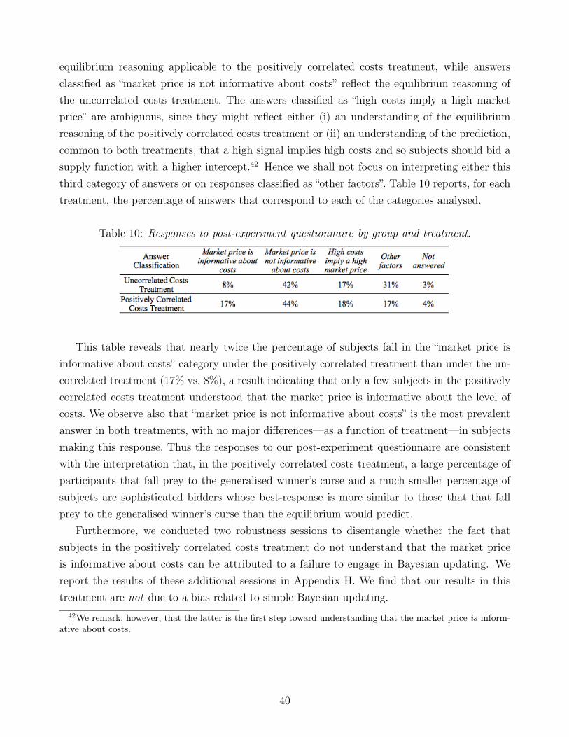
equilibrium reasoning applicable to the positively correlated costs treatment, while answersclassified as “market price is not informative about costs” reflect the equilibrium reasoning ofthe uncorrelated costs treatment. The answers classified as “high costs imply a high marketprice” are ambiguous, since they might reflect either (i) an understanding of the equilibriumreasoning of the positively correlated costs treatment or (ii) an understanding of the prediction,common to both treatments, that a high signal implies high costs and so subjects should bid asupply function with a higher intercept.42 Hence we shall not focus on interpreting either thisthird category of answers or on responses classified as “other factors”. Table 10 reports, for eachtreatment, the percentage of answers that correspond to each of the categories analysed.

Table 10: Responses to post-experiment questionnaire by group and treatment.

This table reveals that nearly twice the percentage of subjects fall in the “market price isinformative about costs” category under the positively correlated treatment than under the un-correlated treatment (17% vs. 8%), a result indicating that only a few subjects in the positivelycorrelated costs treatment understood that the market price is informative about the level ofcosts. We observe also that “market price is not informative about costs” is the most prevalentanswer in both treatments, with no major differences—as a function of treatment—in subjectsmaking this response. Thus the responses to our post-experiment questionnaire are consistentwith the interpretation that, in the positively correlated costs treatment, a large percentage ofparticipants that fall prey to the generalised winner’s curse and a much smaller percentage ofsubjects are sophisticated bidders whose best-response is more similar to those that that fallprey to the generalised winner’s curse than the equilibrium would predict.

Furthermore, we conducted two robustness sessions to disentangle whether the fact thatsubjects in the positively correlated costs treatment do not understand that the market priceis informative about costs can be attributed to a failure to engage in Bayesian updating. Wereport the results of these additional sessions in Appendix H. We find that our results in thistreatment are not due to a bias related to simple Bayesian updating.

42We remark, however, that the latter is the first step toward understanding that the market price is inform-ative about costs.

40

7 Concluding Remarks

We have analysed bidding behaviour in an experiment which reflects the complexity of real-worldmarkets where bidders compete in supply functions, have incomplete information about theircosts, and receive a private signal. We used the unique Bayesian Nash equilibrium prediction andits comparative statics as benchmarks when evaluating the experimental results. Our experimentemployed a between-subjects design with two treatments: uncorrelated costs and positivelycorrelated costs; the former served as our control treatment. In conducting the experiment, wechose numerical values for the model’s parameters that allowed theoretical predictions aboutbehaviour and outcomes to be sufficiently differentiated between the two treatments.

We find that most subjects bid in accordance with the equilibrium predictions in a simplestrategic environment (uncorrelated costs treatment), yet most subjects fail to do so in a morecomplex strategic environment (positively correlated costs treatment) in which they are requiredto use the market price to extract information about the level of costs. On average, subjectsin the positively correlated costs treatment bid flatter supply functions than predicted by theequilibrium. Our findings are consistent with the experimental literature on correlation neglect(see Section 2), a phenomenon that in our setting is intertwined with the generalised winner’scurse. To the best of our knowledge, this paper is the first to document that phenomenon in anenvironment characterised by interdependent values and the auctioning of multiple units of adivisible good.

In electricity markets, mitigating the market power is a primary concern of regulators.43

If costs are positively correlated then our experiment shows that, when a large proportionof subjects who are competing in supply functions neglect the correlation among costs, marketoutcomes are more competitive than in the equilibrium. Yet despite being more competitive, theresulting allocations present a higher productive inefficiency than the corresponding equilibriumallocations.

Our experiment suggests a few open questions for future research, both experimental andtheoretical. Future work could explore mechanisms by which subjects learn to overcome thegeneralised winner’s curse (e.g., asking subjects to come back to the laboratory a few dayslater (experienced bidders); replicating the experiment with professional traders; extending thenumber of rounds). The experimental findings reported here also call for the development oftheoretical models that analyse market competition among participants who exhibit variousdegrees of strategic sophistication—as well as for examination of the convergence properties ofdifferent types of learning models in markets characterised by supply function competition andprivate information.

43See, for example, Hortaçsu and Puller (2008) and Holmberg and Wolak (2015).

41

References

[1] Arellano, M., and Bover, O., (1995), “Another Look at the Instrumental Variable Estima-tion of Error-Components Models,” Journal of Econometrics, 68: 29-51.

[2] Ausubel, L. M., Cramton, P., Pycia, M., Rostek, M., and Weretka, M., (2014), “DemandReduction and Inefficiency in Multi-unit Auctions,” The Review of Economic Studies, 81(4),1366-1400.

[3] Baldick, R., Grant, R., and Kahn, E., (2004), “Theory and Application of Linear SupplyFunction Equilibrium in Electricity Markets,” Journal of Regulatory Economics, 25(2),143-167.

[4] Baltagi, B.H., (2008), Econometric Analysis of Panel Data, 4th ed., Chichester, UK: Wiley.

[5] Bigoni, M., and Fort, M., (2013), “Information and Learning in Oligopoly: An Experiment,”Games and Economic Behavior, 81: 192-214.

[6] Blundell, R., and Bond, S., (1998), “Initial Conditions and Moment Restrictions in DynamicPanel Data Models,” Journal of Econometrics, 87: 115-143.

[7] Bolle, F., Grimm, V., Ockenfels, A., and del Pozo, X., (2013), “An Experiment on SupplyFunction Competition,” European Economic Review, 63(C): 170-185.

[8] Brandts, J., Reynolds, S.S., and Schram, A., (2014), “Pivotal Suppliers and Market Powerin Experimental Supply Function Competition,” The Economic Journal, 124: 887–916.

[9] Brocas, I., Carrillo, J. D., Wang, S.W., and Camerer, C.F., (2014), “Imperfect Choice orImperfect Attention? Understanding Strategic Thinking in Private Information Games,”Review of Economic Studies, 81: 944-970.

[10] Camerer, C. F., (2003), Behavioral Game Theory: Experiments in Strategic Interaction,Princeton University Press.

[11] Camerer, C.F., and Fehr, E., (2006), “When Does “Economic Man” Dominate Social Beha-vior?,” Science, 311: 47-52.

[12] Carrillo, J. D., and Palfrey, T., (2011), “No Trade,” Games and Economic Behavior, 71(1),66-87.

[13] Cassola, N., Hortaçsu, A. and Kastl, J., (2013), “The 2007 Subprime Market Crisis Throughthe Lens of European Central Bank Auctions for Short-Term Funds,” Econometrica, 81:1309–1345.

42

[14] Charness, G., and Levin, D., (2009), “The origin of the winner’s curse: a laboratory study,”American Economic Journal: Microeconomics, 207-236.

[15] Crawford, V. P., and Iriberri, N., (2007), “Level-k Auctions: Can a Nonequilibrium Modelof Strategic Thinking Explain the Winner’s Curse and Overbidding in Private-Value Auc-tions?,” Econometrica, 75(6): 1721-1770.

[16] Dufwenberg, M., and Gneezy, U., (2000), “Price Competition and Market Concentration:An Experimental Study,” International Journal of Industrial Organization, 18, 7-22.

[17] Engelbrecht-Wiggans, R., List, J. A., & Reiley, D. H., (2005), “Demand Reduction inMulti-unit Auctions: Evidence from a Sportscard Field Experiment: Reply,” The AmericanEconomic Review, 95(1), 472-476.

[18] Engelbrecht-Wiggans, R., List, J. A., and Reiley, D. H., (2006)., “Demand Reduction inMulti-Unit Auctions With Varying Number of Bidders: Theory and Evidence from a FieldExperiment,” International Economic Review, 47(1), 203-231.

[19] Enke, B., and Zimmermann, F., (2013), “Correlation Neglect in Belief Formation,” IZADiscussion Paper No. 7372.

[20] Erev, I., and Roth, A., (1998), “Predicting how People Play Games: Reinforcement Learn-ing in Experimental Games with Unique, Mixed Strategy Equilibria,” American EconomicReview, 88: 848–881.

[21] Esponda, I., and Vespa, E., (2014), “Hypothetical Thinking and Information Extraction inthe Laboratory,” American Economic Journal: Microeconomics, 6(4): 180-202.

[22] Eyster, E., and Rabin, M., (2005), “Cursed Equilibrium,” Econometrica, 73(5), 1623-1672.

[23] Fischbacher, U., (1999), “z-Tree 1.1.0: Experimenter’s Manual,” University of Zurich, In-stitute for Empirical Research in Economics.

[24] Fraley, C., and Raftery, A.E. (2002), “Model-based Clustering, Discriminant Analysis, andDensity Estimation,” Journal of the American Statistical Association, 97, 611-631.

[25] Georganas, S., and Nagel, R., (2011), “Auctions with Toeholds: An Experimental Study ofCompany Takeovers,” International Journal of Industrial Organization, 29(1), 34-45.

[26] Goeree, J., and Offerman, T., (2003), “Winner’s Curse Without Overbidding,” EuropeanEconomic Review, 47(4), 625-644.

43

[27] Holmberg, P., and Wolak, F.A., (2015), “Electricity Markets: Designing Auctions WhereSuppliers Have Uncertain Costs,” Cambridge Working Papers in Economics, No. 1541.

[28] Holt, C. A., and Sherman, R., (1994), “The Loser’s Curse,” American Economic Review :642-652.

[29] Hortaçsu, A., and Puller, S. L., (2008), “Understanding Strategic Bidding in Multi-unitAuctions: A Case Study of the Texas Electricity Spot Market,” The RAND Journal ofEconomics, 39: 86–114.

[30] Huck, S., Normann, H.T., and Oechssler, J., (1999), “Learning in Cournot Oligopoly- AnExperiment,” Economic Journal, 109, C-80-90.

[31] Huck, S., Normann, H.T., and Oechssler, J., (2004), “Two are Few and Four are Many:Number Effects in Experimental Oligopolies,” Journal of Economic Behavior and Organ-ization, 53(4): 435-446.

[32] Kagel, J. H., and Levin, D., (1986), “The Winner’s Curse and Public Information in Com-mon Value Auctions,” American Economic Review, 76(5): 894-920.

[33] Kagel, J. H., and Levin, D., (2001), “Behavior in Multi-Unit Demand Auctions: Experi-ments with Uniform Price and Dynamic Vickrey Auctions,” Econometrica, 69(2): 413-454.

[34] Kagel, J. H. and Levin, D., (forthcoming) “Auctions: A Survey of Experimental Research,1995 - 2008,” in The Handbook of Experimental Economics, Volume II , J. H. Kagel and A.E. Roth (eds). Princeton: Princeton University Press.

[35] Keloharju, M., Nyborg, K. G., and Rydqvist, K., (2005), “Strategic Behavior and Underpri-cing in Uniform Price Auctions: Evidence from Finnish Treasury Auctions,” The Journalof Finance, 60(4), 1865-1902.

[36] Klemperer, P., and Meyer, M., (1989), “Supply Function Equilibria in Oligopoly underUncertainty,” Econometrica, 57(6): 1243–1277.

[37] Koch, C., and Penczynski, S., (2015), “The Winner’s Curse: Conditional Reasoning andBelief Formation,” Working paper SSRN No. 2563438.

[38] Levin, D., (2005), “Demand Reduction in Multi-Unit Auctions: Evidence from a SportscardField Experiment: Comment,” The American Economic Review, 95(1): 467-471.

[39] Levy, G., and Razin, R., (2015), “Correlation Neglect, Voting Behavior, and InformationAggregation,” American Economic Review, 105(4), 1634-1645.

44

[40] List, J.A., and Lucking-Reiley, D., (2000), “Demand Reduction in Multi-Unit AuctionsEvidence from a Sportcard Field Experiment,” American Economic Review, 90(4): 961-972.

[41] Lopomo, G., Marx, L. M., McAdams, D., and Murray, B., (2011), “Carbon AllowanceAuction Design: An assessment of Options for the United States,” Review of EnvironmentalEconomics and Policy, 5(1), 25-43.

[42] Nagel, R., (1995), “Unraveling in Guessing Games: An Experimental Study,” AmericanEconomic Review, 85(5): 1313-1326.

[43] Nguyen, M., (2010), “XTSUR: Stata Module to Estimate Seemingly Unrelated RegressionModel on Unbalanced Panel Data,” Statistical Software Component No. S456953, BostonCollege Department of Economics.

[44] Offerman, T., Potters, J., and Sonnemans, J., (2002), “Imitation and Belief Learning in anOligopoly Experiment,” The Review of Economic Studies, 69(4): 973-997.

[45] Sade, O., Schnitzlein, C., and Zender, J.F., (2006), “Competition and Cooperation inDivisible Good Auction: An Experimental Examination,” The Review of Financial Studies,19(1): 195-235.

[46] Samuelson, W. F., and Bazerman, M. H., (1985), “Negotiation under the Winner’s Curse,”Research in Experimental Economics, 3, 105-38.

[47] Selten, R., and Buchta, J., (1999), “Experimental Sealed Bid First Price Auctions with Dir-ectly Observed Bid Functions,” In Games and Human Behavior, Mahwah NJ, L. ErlbaumAssociates Inc., 79-102.

[48] Vives, X., (2008), Information and Learning in Markets: The Impact of Market Micro-structure. Princeton University Press.

[49] Vives, X., (2011), “Strategic Supply Function Competition with Private Information,” Eco-nometrica, 76(3): 1919-1966.

[50] Weizsacker, G., (2010), “Do We Follow Others when We Should? A Simple Test of RationalExpectations,” American Economic Review, 100, 2340-2360.

45

Appendices

Appendix A: Theoretical considerations

This section uses results from Vives (2011). When demand is inelastic and equal q and if−1n−1

< ρ < 1, σ2ε

σ2θ< ∞ and λ > 0, the model described in Section 3 has a unique linear Supply

Function Equilibrium (SFE) given as

X(si, p) = b− asi + cp, (5)

where

a =(1− ρ)σ2

θ

(1− ρ)σ2θ + σ2

ε

(d+ λ)−1, (6)

b =1

1 +M

(qM

n− σ2

ε θ(d+ λ)−1

(1 + (n− 1)ρ)σ2θ + σ2

ε

), (7)

and

c =n− 2−M

λ(n− 1)(1 +M), (8)

where M = ρnσ2ε

(1−ρ)((1+(n−1)ρ)σ2θ+σ2

ε)represents an index of adverse selection and d = 1

(n−1)cis the

slope of the inverse residual demand. The expected intercept is equal to E[f ] = b− aθ.The expected market price is equal to

E[p] = θ +(d+ λ)q

n. (9)

Ex-ante expected profits of seller i at the SFE given the predicted values with full informationare equal to:44

E[π(t; d)] = (d+λ

2)

(q2

n2+

(1− ρ)2(n− 1)σ4θ

n(σ2ε + σ2

θ(1− ρ))

1

(d+ λ)2

), (10)

where t=(E [θ1 | s] , E [θ2 | s] , ..., E [θn | s]), s = (s1, s2, ..., sn) and π(t; d) = 1n

∑i πi(t; d). We

note that xi(t; d) = x(t; d) + t−ti(d+λ)

. Therefore, the first term of expected profits corresponds to

expected profits at the average quantity since they are equal to (p− θ) qn− λ

2( qn)2 = (d + λ

2) q

2

n2 .The second term is related to the dispersion of the predicted values. For each subject and round,we compute profits conditional on the private signal. We then calculate the average profits in

44At the SFE the market price and the signal provide sufficient information on the joint information of themarket.

1

each treatment, which give us an estimate for ex-ante expected profits.In terms of the efficiency at the equilibrium allocation, we note the following. First, there is noaggregate inefficiency since the demand is inelastic. Second, the ex-ante expected deadweightloss, E[DWL], at the equilibrium allocation is the difference between expected total surplus atthe efficient allocation and at the equilibrium allocation. We can write it as

E[DWL] =nλ

2E[(xi − xoi )2]. (11)

Vives (2011) shows that the efficient allocation is equal to

xoi =q

n+

(1− ρ)σ2θ

λ((1− ρ)σ2θ + σ2

ε )(s− si), (12)

and that expected deadweight loss at the equilibrium allocation can be then written as

E[DWL] =λ

2(1

λ− 1

λ+ d)2 (1− ρ)2(n− 1)σ4

θ

(σ2ε + σ2

θ(1− ρ)). (13)

For each market we compute the empirical counterpart of the (interim) deadweight loss at theexperimental allocation as follows

dwl = (nλ

2)(

1

n

n∑i=1

(xei − xoi )2), (14)

where xei is the experimental allocation (superscript e is to differentiate it from the equilibriumallocation, xi) and xoi is the efficient allocation as defined above. In order to calculate theaverage deadweight loss in each treatment, we average the interim deadweight losses for the600 markets in each treatment, which gives us an estimate for the ex-ante expected deadweightloss.45

Appendix B: Equilibrium predictions, ex-ante expected out-

comes, and statistical distribution of random costs and er-

rors used in the experiment

In our experiment, given the experimental parameters of Table 2, the numerical equilibriumsupply function and ex-ante expected outcomes in the two treatments can be summarised inthe table below.

45There are 600 markets in each treatment since we have 6 groups, which consist of 4 markets each for 25rounds.

2

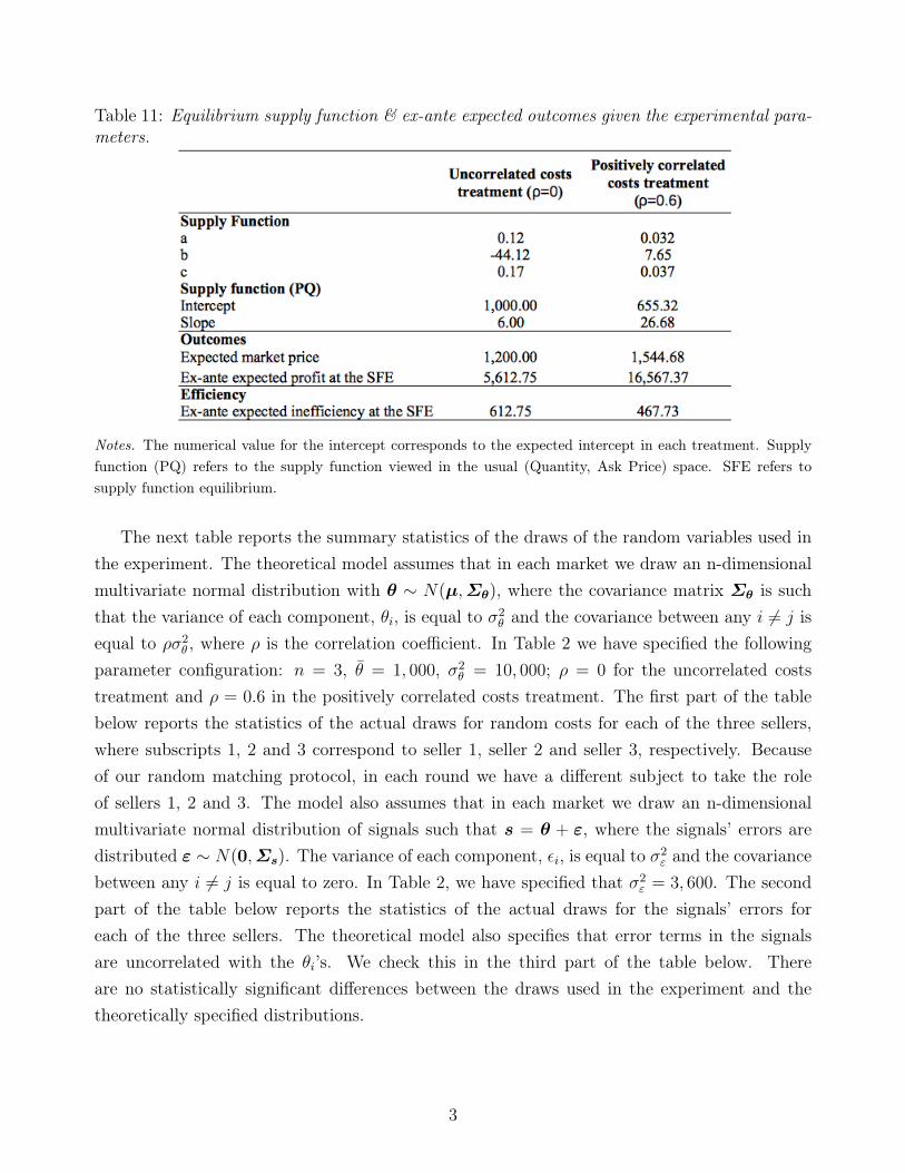
Table 11: Equilibrium supply function & ex-ante expected outcomes given the experimental para-meters.

Notes. The numerical value for the intercept corresponds to the expected intercept in each treatment. Supplyfunction (PQ) refers to the supply function viewed in the usual (Quantity, Ask Price) space. SFE refers tosupply function equilibrium.

The next table reports the summary statistics of the draws of the random variables used inthe experiment. The theoretical model assumes that in each market we draw an n-dimensionalmultivariate normal distribution with θ ∼ N(µ,Σθ), where the covariance matrix Σθ is suchthat the variance of each component, θi, is equal to σ2

θ and the covariance between any i 6= j isequal to ρσ2

θ , where ρ is the correlation coefficient. In Table 2 we have specified the followingparameter configuration: n = 3, θ = 1, 000, σ2

θ = 10, 000; ρ = 0 for the uncorrelated coststreatment and ρ = 0.6 in the positively correlated costs treatment. The first part of the tablebelow reports the statistics of the actual draws for random costs for each of the three sellers,where subscripts 1, 2 and 3 correspond to seller 1, seller 2 and seller 3, respectively. Becauseof our random matching protocol, in each round we have a different subject to take the roleof sellers 1, 2 and 3. The model also assumes that in each market we draw an n-dimensionalmultivariate normal distribution of signals such that s = θ + ε, where the signals’ errors aredistributed ε ∼ N(0,Σs). The variance of each component, εi, is equal to σ2

ε and the covariancebetween any i 6= j is equal to zero. In Table 2, we have specified that σ2

ε = 3, 600. The secondpart of the table below reports the statistics of the actual draws for the signals’ errors foreach of the three sellers. The theoretical model also specifies that error terms in the signalsare uncorrelated with the θi’s. We check this in the third part of the table below. Thereare no statistically significant differences between the draws used in the experiment and thetheoretically specified distributions.

3

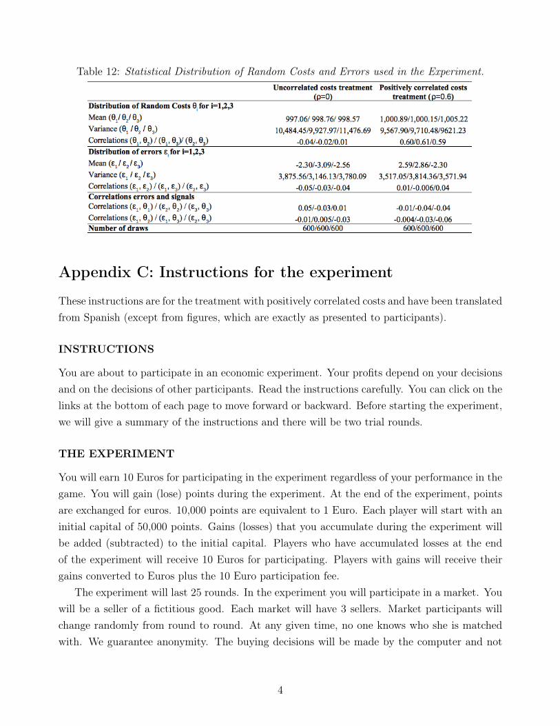
Table 12: Statistical Distribution of Random Costs and Errors used in the Experiment.

Appendix C: Instructions for the experiment

These instructions are for the treatment with positively correlated costs and have been translatedfrom Spanish (except from figures, which are exactly as presented to participants).

INSTRUCTIONS

You are about to participate in an economic experiment. Your profits depend on your decisionsand on the decisions of other participants. Read the instructions carefully. You can click on thelinks at the bottom of each page to move forward or backward. Before starting the experiment,we will give a summary of the instructions and there will be two trial rounds.

THE EXPERIMENT

You will earn 10 Euros for participating in the experiment regardless of your performance in thegame. You will gain (lose) points during the experiment. At the end of the experiment, pointsare exchanged for euros. 10,000 points are equivalent to 1 Euro. Each player will start with aninitial capital of 50,000 points. Gains (losses) that you accumulate during the experiment willbe added (subtracted) to the initial capital. Players who have accumulated losses at the endof the experiment will receive 10 Euros for participating. Players with gains will receive theirgains converted to Euros plus the 10 Euro participation fee.

The experiment will last 25 rounds. In the experiment you will participate in a market. Youwill be a seller of a fictitious good. Each market will have 3 sellers. Market participants willchange randomly from round to round. At any given time, no one knows who she is matchedwith. We guarantee anonymity. The buying decisions will be made by the computer and not

4

a participant of the experiment. In each round and market, the computer will buy exactly 100units of the good.

YOUR PROFITS

In each round, your profits are calculated as shown in the figure below:46

Your profits are equal to the income you receive from selling units minus total costs (con-sisting of production and transaction costs).

Some details to keep in mind: you only pay the total costs of the units that you sell. If yousell zero units in a round, your profits will also be zero in this round. You can make losses whenyour income is less than the total costs (production and transaction). The cumulative profitsare the sum of the profits (losses) on each round. Losses will be deducted from the accumulatedprofits. Throughout the experiment, a window in the upper left corner of your screen will showthe current round and accumulated profits.

YOUR DECISION

In each round, you have to decide the minimum price that you are willing to sell each unit for.We call these Ask Prices.

THE MARKET PRICE

Once the three sellers in a given market have entered and confirmed their decisions, the computercalculates the market price as follows.

1. In each market, the computer observes the 300 Ask Prices introduced by the sellers ofyour market.

2. The computer ranks the 300 Ask Prices from the lowest to the highest.46English explanation: the top part of the figure explains the formula for profits given in equation (1). The

bottom part of the figure expresses Profits=Revenues-Production Costs-Transaction Costs.

5

3. The computer starts buying the cheapest unit, then it buys the next unit, etc. until ithas purchased exactly 100 units. At this time the computer stops.

4. The Ask Price of the 100th unit purchased by the computer is the market price (the priceof the last unit purchased by the computer).

The market price is the same for all units sold in a market. In other words, a seller receivesa payment, which is equal to the market price for each unit she sells. If more than one unit isoffered at the market price, the computer calculates the difference:

Units Remaining= 100- Units that are offered at prices below the market price.The Units Remaining are then split proportionally among the sellers that have offered them

at an Ask Price equal to the market price.

UNITS SOLD

In each round and market, the three sellers offer a total of 300 units. The computer purchasesthe 100 cheapest units. Each seller sells those units that are offered at lower Ask Prices thanthe market price. Note that those units that are offered at higher Ask Prices than the marketprice are not sold. Those units offered at an Ask Price which is equal to the market price willbe divided proportionally among the sellers that have offered them.

MARKET RULES

In each round and market, the computer buys exactly 100 units of the good at a price notexceeding 3.600. In order to simplify the task of entering all Ask Prices in each round, werequest that you to enter:

• Ask Price for Unit 1

• Ask Price for Unit 2

Ask Prices can be different for different units. To find Ask Prices for the other units, we willjoin the Ask Price for Unit 1 and the Ask Price for Unit 2 by a straight line. In this way, we findthe Ask Prices for all the 100 units. In the experiment, you will be able to see this graphicallyand try different values until you are satisfied with your decision.

We apply the following five market rules.1. You must offer all the 100 units for sale.2. Your Ask Price for one unit must always be greater than or equal to the Ask Price of the

previous unit. Therefore, the Ask Price for the second unit cannot be less than the Ask Pricefor the first unit. You can only enter integers for your decisions.

3. Both Ask Prices must be zero or positive.4. The buyer will not purchase any unit at a price above the price cap of 3,600.

6

5. The Ask Price for some units may be lower your unit cost, since unit costs are unknownat the time when you decide the Ask Prices. You may have losses.

EXAMPLE

This example is illustrative and irrelevant to the experiment itself. We give the example onpaper. Here you can see how the computer determines the market price and units sold by eachseller in a market.

UNIT COST

In each round the unit cost is random and unknown to you at the time of the decision. The unitcost is independent of previous and future round. Your unit cost is different from the unit costof other participants. However, your unit cost is related to the unit costs of the other marketparticipants. Below we explain how unit costs are related and we give a figure and explanationof the possible values of unit costs and their associated frequencies. This figure is the same forall sellers and all round.47

The horizontal displays the unit cost while the vertical axis shows the frequency with whicheach unit cost occurs (probability). This frequency is indicated by the length of the correspond-ing bar.

In the figure you can see that the most frequent unit cost is 1,000. We obtain 1,000 as unitcost with a frequency of 0.35%. In general terms, we would obtain a unit cost of 1,000 in 35 of1,000 cases.

In 50% of the cases (50 of 100 cases), the unit cost will be between 933 and 1,067.In 75% of the cases (75 of 100 cases), the unit cost will be between 885 and 1,115 .

47English explanation: the figure shows the possible values of costs θi (horizontal axis) and their correspondingprobabilities (vertical axis).

7

In 95% of the cases (95 of 100 cases), the unit cost will be between 804 and 1,196 .There is a very small chance that the unit cost is less than 700. This can occur in 1 of 1,000

cases approximately. Similarly, there is a very small chance that the unit cost is greater than1,300. This occurs can occur in 1 of 1,000 cases, approximately.

For participants with knowledge of statistics: the unit cost is normally distributed withmean 1,000 and standard deviation 100.

INFORMATION ABOUT YOUR UNIT COST (YOUR SIGNAL)

In each round, each participant receives information on her unit costs. This information is notfully precise. The signal that you receive is equal to:

Signal = UnitCost+ Error

The error is independent of your unit cost, it is also independent from the unit costs of otherparticipants and it is independent from past and future errors. The following figure describesthe possible values of the error term and an indication of how likely each error is likely to occur.This graph is the same for all sellers and rounds.48

On the horizontal axis you can observe the possible values of the error terms. On the verticalaxis, you can observe the frequency with which each error occurs (probability). This frequencyis indicated by the length of the corresponding bar.

In the figure you can see that the most common error is 0. The frequency of error 0 is 0.66%. In general terms, this means that in approximately 66 of 10.000 cases you would get an errorequal to 0.

In 50% of the cases (50 of 100 cases), the error term is between -40 and 40.In 75% of the cases (75 of 100 cases), the error is between -69 and 69.

48English explanation: the figure shows the possible values of the signal’s error (horizontal axis) and theircorresponding probabilities (vertical axis).

8

In 95% of the cases (95 of 100 cases), the error is between -118 and 118.There is a very small chance that the error is less than -200. This occurs in 4 out of 10,000

cases. Similarly, there is a very small probability that the error is greater than 200. This occursin 4 out of 10,000 cases.

For participants with knowledge of statistics: the error has a normal distribution with mean0 and standard deviation 60.

HOW YOUR COST IS RELATED TO THE COSTS OF THE OTHER SELLERS

The unit cost is different for each seller and your unit cost is related to the unit cost of theother sellers in your market. The association between your unit cost and unit cost of anotherseller in your market follows the trend:

• The higher your unit cost, the higher will be the unit cost of the other sellers.

• The lower your unit cost, the lower the unit cost of the other sellers.

The strength of the association between your unit cost and unit cost of another seller is measuredon a 0 to 1 scale. The strength of the association between your unit cost and unit cost of theother seller is +0.6 .49

Graphically we can see the relationship between your unit cost (horizontal axis) and theunit cost of another seller (vertical axis) for some strengths of association. The figure that hasa red frame corresponds to an intensity of association of +0.6.

For participants with knowledge of statistics: the correlation between your unit cost andunit cost of any other player is +0.6 .

49English explanation: the figure explains the meaning of correlation equal to 0, 0.6 and 1.

9

END OF ROUND FEEDBACK

At the end of each round, we will give you information about:

• Your profits (losses) and its components (Revenue-Cost of Production - Cost of transac-tion)

• Market price

• Your units sold

• Other market participants feedback: decisions; profits and unit costs.

You can also check your historical performance in a window in the upper right corner of yourscreen. During the experiment the computer performs mathematical operations to calculate themarket price, units sold, Ask Prices for intermediate units, etc. For these calculation we use allavailable decimals. However, we show all the variables rounded to whole numbers, except fromthe market price.

THE END

This brings us to the end of the instructions. You can take your time to re-read the instructionsby pressing the BACK button. When you understand the instructions you can indicate it to usby pressing the OK button at the bottom of the screen. Next you have to answer a questionnaireabout the instructions, unit cost distributions and signals. When all participants have takenthe questionnaire and indicated OK, we will start the practice rounds. Your profits or losses ofthe practice rounds will not be added or subtracted to your earnings during the experiment.

Appendix D: Comprehension test and experimental screen-

shots

The first part of this appendix reports the comprehension questionnaire which was administeredbefore the trial rounds.

Comprehension Test

Questions. Answer True or False.

1. The unit cost has the same value for each of the participants in your market.

2. The unit cost has the same value for each of the participants in your market.

10

3. If my unit cost is high, it is rather likely that the unit cost of another seller is high.

4. Unit costs between 1000 and 1200 occur with the same frequency than unit costs between1000 and 700.

5. Unit costs larger than 1000 occur with the same frequency as unit costs smaller than 1000.

6. Errors larger than 0 occur more frequently than errors smaller than 0.

7. An error of 5 is the most frequent error.

8. The seller who sells most units will always have the highest profit.

9. If my unit cost is low, it is rather likely that the unit cost of another seller is high.

10. The market price is the same for all units and sellers.

Answers (True (T) and False (F)): Q1. F Q2. T Q3. T (treatment 0.6); F (treatment 0)Q4. F Q5. T Q6. F Q7. F Q8. F Q9. F Q10. T

Notes: These notes appeared on the screen if a participant answered wrongly any of theprevious questions.

Q1. Treatment 0.6: Your unit cost is different from the unit cost of other participants butit is related. Treatment 0: Your unit cost is different from the unit cost of other participants.There is no relation between your unit cost and that of other participants.

Q2. In each round, the unit cost is random and independent from the unit cost of past andfuture rounds.

Q3. Treatment 0.6: The higher your unit cost, the higher the unit cost of the other sellerswill tend to be. Treatment 0: There is no relation between your unit cost and that of otherparticipants. Therefore, if my unit cost is high, I can not deduce anything from the unit costof the other participants.

Q4. Unit costs between 1000 and 1200 occur with higher frequency than unit costs between1000 and 700.

Q5. The unit cost of 1000 is the most frequent one. Unit costs larger than 1000 occur withthe same frequency as unit costs smaller than 1000.

Q6. Errors larger than 0 occur with the same frequency as errors smaller than 0.Q7. An error of 0 is the most frequent error.Q8. Profit does not only depend on the number of units sold. Remember that: Profit =

(MarketPrice− UnitCost)UnitsSold− 1.5UnitsSold2.Q9. Treatment 0.6: The lower your unit cost, the lower the unit cost of the other sellers

will tend to be. Treatment 0: There is no relation between your unit cost and that of other

11

participants. Therefore, if my unit cost is high, I can not deduce anything about the unit costof the other participants.

Q10. The market price is the same for all units and sellers in a market.

The second part of this appendix reports the screenshots used during the experiment.

Screen 1: signal screen50

50English explanation: the first part of the screen reminds participants of the definition of the signal. Thesecond part gives the participant the realisation of her signal for the current round.

12

Screen 2: decision screen51

Screen 3: feedback about a seller’s own performance52

51English explanation: First, the screen reminds the participant of the realisation of her signal for the currentround. Second, it asks the participant to enter the ask price for the first unit and the ask price for the secondunit. The participant has access to a calculator and can see a graphical representation of the supply schedule.The participant can try a few decisions before it presses the “Confirm” button.

52English explanation: this screen reports the participants’ profits/losses in the current round and splits theminto revenues (price multiplied by units sold), production costs (cost multiplied by units sold) and transactioncosts (1.5 multiplied by the square of units sold). The screen displays them both graphically and numerically.

13

Screen 4: feedback about market performance and other sellers’ in the

same market53

Appendix E: Post-experiment questionnaire

After the rounds were completed, we asked for 3 demographic questions: age, gender and degreestudying.We then asked the following additional questions regarding understanding of the game.1. Do you think that a high market price generally means GOOD/MIXED/BAD news aboutthe level of your costs?2. Explain your answer.3. Do you think that the other sellers have answered the same as you to the previous question?4. Explain your answer.

53English explanation: this screen gives the participant feedback about: own supply function and supplyfunctions of the rivals (graphically); units sold by each of the players; the own value of θi and that of the tworivals; profits/losses for each of the players in the market.

14

Appendix F: Analysis of variance of experimental outcomes

and decomposition of deadweight loss

The following table shows the analysis of variance for experimental outcomes and deadweightlosses in each treatment.

Table 13: Analysis of variance of experimental outcomes and deadweight losses.

Note. s.d. refers to standard deviation. The explanation of the variables reported in the table is as follows: s.d.Overall subject level: the variation of individual choice across all rounds; s.d. Between subjects: the variation ofthe individual choice averaged across all rounds; s.d. Within Subjects: the variation within subject over time;s.d. Overall group level: the variation the average choice of the group across all rounds; s.d. Between groups:the variation of the average choice of the group averaged across all rounds; s.d. Within groups: the variationwithin groups over time; and s.d. Overall Treatment level: the variation of the average choice of the treatmentacross all rounds.

The following graph illustrates how the components of deadweight loss combine in eachtreatment.

15

Figure 10: Components of deadweight loss at the experimental allocation in each treatment.

Notes. This graph corresponds to the decomposition of deadweight loss, dwl = (λ2 )(∑ni=1(x

ei −

qn )

2+(xoi −qn )

2−2(xei −

qn )(x

oi −

qn )). The first term is variance of units sold, the second is the variance of the efficient allocation,

and the third is -2 multiplied by the covariance of units sold and the efficient allocation. The bars associatedwith “Sum of components” refer to the sum (

∑ni=1(x

ei −

qn )

2 + (xoi −qn )

2 − 2(xei −qn )(x

oi −

qn )). dwl refers to

deadweight loss.

The next table displays the components of deadweight loss at both the equilibrium and experi-mental allocations in each treatment.

16

Table 14: Components of Deadweight Loss at the equilibrium and experimental allocations ineach treatment.

Notes. Alloc. refers to allocation. In order to calculate dwl in rows (5) and (9), we have used the actualdistribution of draws of the random variables used in the experiment.

Appendix G: Panel data analysis

In this section we present the results of panel data analysis, which is based on the individualchoice or outcome across rounds. For that purpose, we use a random effects panel data ap-proach.54

First, we evaluate whether there is a difference—between the positively correlated coststreatment and the (control) uncorrelated costs treatment—with regard to either market be-haviour or outcomes. Table 15 reports random effects regression results of jointly estimating,for our panel data, the equation for the supply function slope and the intercept. The so-calledseemingly unrelated regression (SUR) method we use, which assumes that disturbances acrossequations may be correlated, yields efficient estimates.55 In Table 15[1], we jointly estimate the

54For market price and deadweight loss, the unit of analysis is the market across rounds.55See Baltagi (2008) for the theoretical background on this estimation.

17

following set of equations:

SlopePQ it = β0S + β1SD_Treatment i +∑j

βjD_Groupij + νi + uit;

InterceptPQ it = β0I + β1ID_Treatment i +∑j

βiD_Groupj + wi + vit.

Here the subscripts S and I signify (respectively) slope and intercept, the subscript it denotesthe choice of subject i at round t, and j is an index for the group to which a subject belongs. Theterm D_Treatment is an indicator variable that takes the value 0 (resp., 1) for the uncorrelated(resp., positively correlated) costs treatment, and the D_Groupij are a set of dummies thattake the value 1 if subject i belongs to group j (and value 0 otherwise). The terms uit and vitare observation-specific errors; νi and wi are unobserved individual effects.

In Table 15[2] we report results from the following set of augmented regressions:

SlopePQ it = β0S + β1SD_Treatment i +∑j

D_Groupij + β2St

+ β3S(D_Treatment i × t) + β4SSignal it + νi + uit;

InterceptPQ it = β0I + β1ID_Treatment i +∑j

D_Groupij + β2It

+ β3I(D_Treatment i × t) + β4ISignal it + wi + vit.

In these expressions, t isa variable for the round number, D_Treatment × t is the interactionterm between the round number and treatment, and Signal is the signal received by subject iat round t. The errors uit and vit are correlated across equations.

18

Table 15: Panel data: SUR of random effects.

Note. Each equation was estimated with group dummies; standard errors are given in parenthesises. Thisestimation was performed via the xtsur command in Stata (cf. Nguyen 2010), which is used for one-way randomeffects estimation of seemingly unrelated regressions (SURs) in a panel data set. Note that the xtsur commanddoes not allow for clustered standard errors.*, **, and *** denote significance at (respectively) the 10%, 5%, and 1% levels.

In both Table 15[1] and Table 15[2] we see that D_Treatment is not statistically significantregardless of whether it is the only regressor or whether we also control for additional variables.With regard to the regression for the supply function slope, from Table 15[2] we can drawthe following conclusions: round has a significant and negative coefficient, which means thatsupply functions become flatter as the number of rounds increases; and D_Treatment × t hasa significant and positive coefficient, which means that the decrease in the slope of the supplyfunction is less pronounced in the positively correlated costs treatment. We also find thatSignal is not statistically significant in determining the supply function slope. With regardto the regression for the supply function intercept, we may conclude as follows: round has asignificant and positive coefficient, which means that the supply function intercept increases asthe number of rounds increases; D_Treatment× t has a significant and negative coefficient thatis nearly identical to the coefficient for round, which means that the supply function interceptdoes not vary as a function of round in the positively correlated costs treatment; and Signal, aspredicted by the theoretical model, has a significant and positive coefficient.

Second, we estimate a panel with random effects and where standard errors are clustered atthe group level for the dependent variables (market prices, profits, and deadweight losses). InTable 16[1] we estimate the following equation for market price:

MarketPricemt = β0 + β1D_Treatmentm + νm + ωmt.

Here the subscript mt denotes market m at round t; εmt is the error term; νm is the random

19

effect, which is uncorrelated with the regressor; and D_Treatment is the treatment dummydefined previously. In Table 16[2], we augment the regression with additional controls andestimate the following equation:

MarketPricemt = β0 + β1D_Treatmentm + β2t

+ β3(D_Treatmentm × t) + β4Signalmt + νm + ωmt,

where the unit of observation is the market across time and where all the variables are as definedbefore.

The results reported in Table 16[1] show that D_Treatment is not statistically significant—either when the treatment dummy is used as the only regressor or when we include the additionalcontrols. In Table 16[2] we observe that, with respect to determining market price, the signalreceived is the only variable with a positive and significant coefficient.

Table 16: Panel data: Regression of random effects for market outcomes and deadweight loss.

Note. This estimation was performed using the xtreg, re command in Stata. Standard errors (s.e.), reported inparentheses, are clustered at the group level.*, **, and *** denote significance at (respectively) the 10%, 5%, and 1% levels.

Third, for profits we use the same panel data approach as for market price—but now the unitof observation is the subject across rounds.56 We find that D_Treatment is not significant inthe results of either Table 16[3] or Table 16[4]. The signal received has a negative and significantcoefficient, reflecting the negative correlation between signal (and also unit costs) and profits. Inaddition, we find that profits increase slightly across rounds in the uncorrelated costs treatment;in the positively correlated costs treatment, however, there is no evolution of profits (in eitherdirection) across rounds.

56In Table 16[3], we estimate the equation Profit it = β0 + β1D_Treatment i + νi + ωit, where the subscript itsignifies subject i at round t and where εit is the error term. In Table 16[4], we augment that regression asfollows: Profit it = β0 + β1D_Treatment i + β2t + β3(D_Treatment i × t) + β4Signal it + νi + ωit.

20

Fourth, for deadweight loss we use the same same panel data approach as for market price.57

The results presented in Table 16[5] and Table 16[6] show that D_Treatment is not statisticallysignificant. Yet we do find that, in both treatments, deadweight losses decline across rounds; thisresult indicates that allocations become more efficient as the subjects gain bidding experience.

In short: all panel data results are consistent with the stylised facts and with the testspresented in the Section 5.

Appendix H: Best-response analysis

This section uses the notation of the theoretical background presented in Section 3 and com-putes a seller’s best-response strategy given arbitrary strategies of rivals. We assume that anagent knows the strategies of the rivals, and that she forms correct beliefs about events in thecompetitive and information environments. The best-response strategy of seller i can be writtenas Xi(si, p) = bi−aisi + cip, and the actual strategies of the rivals as Xj(sj, p) = bj−ajsj + cjp,where j 6= i. The rivals’ average supply function slope is c−i = 1

n−1

∑i 6=j cj, and the rivals’

average fixed part of the intercept is b−i = 1n−1

∑j 6=i bj. Furthermore, for simplicity, we assume

that all rivals set the same response to private information, i.e. aj = a−i for all j 6= i.Lemma 1 determines agent i ’s best-response strategy given arbitrary strategies of the rivals.

The assumptions required for Lemma 1 to hold are consistent with the features of our experi-mental design.

Lemma 1: Best-response strategy

Assume that ρ ∈ [0, 1) and that the rivals’ average supply function is characterisedby (a−i, b−i,, c−i). Suppose that rivals set a supply function such that c−i > 0 andthat all rivals set the same response to private information such that aj = a−i > 0

for all j 6= i. The best-response strategy for seller i is then given as:

ai =R

di + λ+ Ti, (15)

bi =(θ(R + Ti(n− 1)a−i − 1) + Ti(q − (n− 1)b−i))

di + λ+ Ti, (16)

57In Table 16[5] we estimate the following equation for deadweight loss: dwlmt = β0 + β1D_Treatmentm +νm + ωmt, where again the subscript mt denotes market m at round t and εmt is the error term. In Table 16[6],we augment the regression with additional and estimate the following equation: dwlmt = β0+β1DT reatmentm+β2t + β3(D_Treatmentm × t) + β4Signalmt + νm + ωmt.

21

ci =1− Ti(n− 1)c−idi + λ+ Ti

, (17)

where di = 1(n−1)c−i

, R =σ2θ(σ2

θ(1−ρ)(1+(n−1)ρ)+σ2ε )

(σ2θ(1−ρ)+σ2

ε )(σ2θ(1+(n−1)ρ)+σ2

ε ), and

Ti =ρσ2θσ

2ε

(σ2θ(1−ρ)+σ2

ε )(σ2θ(1+(n−1)ρ)+σ2

ε )a−i.

Proof: Given the strategies of the rivals, seller i maximises her profits and the first ordercondition is given as: Xi(si, p) = p−E[θ|si,p]

(di+λ). Market clearing implies that q =

∑nj=1 X(sj, p), and

given the definitions of b−i, c−i and the assumption that aj = a−i for all j 6= i, we can re-writethe market clearing expression as: p(n− 1)c−i = q − (n− 1)b−i + a−i

∑i 6=j sj − xi. Then define

di = 1(n−1)c−i

and Ii = q − (n − 1)b−i + a−i∑

i 6=j sj so that we can write p = Ii − dixi. All theinformation contained in p is also contained in hi, where hi = a−i

∑j 6=i sj and can be shown to

be equal to hi = (n − 1)b−i − q + (n − 1)c−ip + xi. The second order condition is satisfied if2di + λ > 0, which is always satisfied if c−i > 0.

We can now find an expression for E[θi | si, p] = E[θi | si, hi]. The mean of the vector

θi

si

hi

is equal to

θ

θ

a−i(n− 1)θ

and the variance-covariance matrix is:

σ2θ σ2

θ ρσ2θa−i(n− 1)

σ2θ σ2

θ + σ2ε ρσ2

θa−i(n− 1)

ρσ2θa−i(n− 1) ρσ2

θa−i(n− 1) a2−i(n− 1)((σ2

ε + σ2θ) + (n− 2)ρσ2

θ)

Using the expressions for conditional expectations of normally distributed random variables, weobtain:

E[θi | si, hi] = θ +R(si − θ) + Ti(hi − (n− 1)a−iθ), (18)

where

R =σ2θ(σ

2θ(1− ρ)(1 + (n− 1)ρ) + σ2

ε )

(σ2θ(1− ρ) + σ2

ε )(σ2θ(1 + (n− 1)ρ) + σ2

ε ), (19)

and

Ti =ρσ2

θσ2ε

(σ2θ(1− ρ) + σ2

ε )(σ2θ(1 + (n− 1)ρ) + σ2

ε )a−i. (20)

In order to obtain the best-response strategy for seller i, we first equate the coefficient onthe signal, si and obtain: ai = R−Tiai

(di+λ), or equivalently: ai = R

di+λ+Ti. Second, we equate

22

the coefficient on the price and obtain: ci = 1−Ti(n−1)c−i−Tici(di+λ)

. Grouping terms with ci, weobtain: ci = 1−Ti(n−1)c−i

(di+λ+Ti). Third, we equate the coefficient on the constant and obtain: bi =

θ(R+Ti(n−1)a−i−1)+Ti(q−(n−1)b−i)(di+λ+Ti)

. �The next Lemma describes the comparative statics of agent i’s best-response function.

Lemma 2: Strategic incentives

Assume that ρ ∈ [0, 1) and that the rivals’ average supply function is characterisedby (a−i, b−i,, c−i). Suppose that rivals bid a supply function such that c−i > 0 andthat all rivals set the same response to private information such that aj = a−i > 0

for all j 6= i.

If ρ = 0 then: ∂ai∂a−i|c−i=const= 0, ∂bi

∂b−i|a−i=const,c−i=const= 0 and ∂ci

∂c−i|a−i=const> 0.

If ρ > 0 then: ∂ai∂a−i|c−i=const> 0, ∂bi

∂b−i|a−i=const,c−i=const< 0,

∂ci∂c−i|a−i=const> 0 for 0 < c−i < c∗−i, where c∗−i is a positive number

and ∂ci∂c−i|a−i=const< 0 for c−i > c∗−i.

Proof: We first evaluate:

∂ci∂c−i

|a−i=const=−Ti(n− 1)2(λ+ Ti)(c−i)

2 − 2Ti(n− 1)c−i + 1

(n− 1)(c−i)2(di + λ+ Ti)2. (21)

since ∂di∂c−i

= −1(n−1)(c−i)2

. When ρ = 0 then Ti = 0 and ∂ci∂c−i|a−i=const> 0. When ρ > 0 then Ti > 0

and the numerator is a polynomial of degree two in c−i, which can be written as:

f(c−i) = −Ti(n− 1)2(λ+ Ti)(c−i)2 − 2Ti(n− 1)c−i + 1 (22)

The maximum of this polynomial occurs at cmax−i = −1(n−1)(λ+Ti)

< 0 and the parabola opensdownwards since the coefficient on (c−i)

2 is negative. The polynomial has a positive (c∗−i) anda negative root. Since we have assumed that c−i > 0, we note that ∂ci

∂c−i|a−i=const> 0 for

0 < c−i < c∗−i and∂ci∂c−i|a−i=const< 0 for c−i > c∗−i.

Second, we take the derivative of ai with respect to a−i. When ρ = 0 then ∂ai∂a−i|b−i=const,c−i=const

=

0. When ρ > 0 then

∂ai∂a−i

|c−i=const=−R

(di + λ+ Ti)2

∂Ti∂a−i

> 0 (23)

since ∂Ti∂a−i

< 0.

23

Third, we take the derivate of bi with respect to b−i. When ρ = 0 then ∂bi∂b−i|a−i=const,c−i=const= 0.

When ρ > 0 then

∂bi∂b−i

|a−i=const,c−i=const=−Ti(n− 1)

di + λ+ Ti< 0 (24)

�

In the experiment, for each two dimensional choice, we observe a subject’s supply functionslope and intercept. Concerning the intercept, we cannot separately observe the two componentsof the supply function’s intercept: response to the private signal and fixed part. This issue hasconsequences for the computation of the best-response to the rivals’ supply function in thepositively correlated costs treatment, where we need to have an estimate of the rivals’ responseto the private signal, a−i. We make the assumption that all sellers equally and optimallyrespond to the private signal, i.e. aj = a−i for all j 6= i. Introducing this assumption into thebest-response strategy, we obtain: aj = a−i =

(1−ρ)σ2θ

(1−ρ)σ2θ+σ2

ε(di + λ)−1.

The figure below illustrates the best-response slope, ci, as a function of the rivals’ averageslope, c−i, in each treatment (with the supply function viewed in (Ask Price, Quantity) space).

Figure 11: Best-response supply function slope as a function of the rivals’ average supply func-tion slope in each treatment and the corresponding equilibrium predictions in the (Ask Price,Quantity) space.

Note. The supply function is viewed in the (Ask Price, Quantity) space, which inverts the axes in relation tomost of the figures shown throughout the text. Note that a steep supply function has a low c when representedin the (Ask Price, Quantity).

24

Appendix I: Cluster analysis

The next table presents the results of cluster analysis in the intermediate time periods in groupsof five rounds.

Table 17: Cluster analysis for the intermediate time periods.

Note. The numbers in parenthesis below the average correspond to standard deviations (s.d.). The equilibriumSF has been calculated using the average signal realisation.

25

The following table summarises the average difference between the experimental supplyfunction and the theoretical best-response supply function in each cluster.

Table 18: Difference between the average experimental and best-response supply function in eachcluster.

Note. The numbers in parenthesis correspond to the standard deviations. The theoretical best-response hasbeen calculated for each individual supply function choice and then averaged for subjects in a particular clusterand time period (blocks of 5 rounds). In order to calculate these averages, we have excluded the choices whichhad a best-response which was unfeasible for subjects in the experiment (73 observations).

Appendix H: Robustness check. Bayesian updating

One could argue that subjects fail to engage in Bayesian updating and that this is why, in thepositively correlated costs treatment, they fail to understand that the market price is informativeabout costs. To explore this possibility further and to assist subjects in the decision-makingprocess, we conducted an additional session with two groups in the positively correlated coststreatment. These sessions had the same experimental design features as in the baseline treatmentbut with three exceptions as follows. First, in addition to the signal received, each subjectreceived the expected value of her own costs—and of her rivals’ costs—conditional on the signal

26

received (thus subject i received a signal si and was also given E[θi | si] and E[θj | si] fori 6= j).58 Second, we explicitly asked each subject to think about what her rivals would doand provided a simulation tool that subjects could use to make a provisional decision, basedon those beliefs, and then visualise the resulting market price; the participant could then reviseher decision. Third, the experiment lasted for 15 (rather than 25) rounds.59 The following tablepresents the summary statistics of outcomes and choices of these two groups in the positivelycorrelated costs treatment.

Table 19: Robustness session: behaviour and outcomes (positively correlated costs treatment).

We find that the average supply function and outcomes in the robustness session are similarto the averages of the baseline treatments, presented in Tables 3 and 5, that correspond to thepositively correlated costs treatment. In other words: assisting subjects in their decision-makingprocess seemed not to have a significant effect, in the positively correlated costs treatment, oneither their behaviour or the experimental outcomes.

Our interpretation—namely, subjects in the positively correlated costs treatment fail tounderstand that the market price is related to the level of their costs and hence that theyshould bid less aggressively—is robust.

58The participant instructions for these additional treatments are available upon request. We explained con-ditional expectations by telling subjects that, in each round, an expert would give them the expected value ofboth their and their rivals’ unit cost.

59We reduced the number of rounds because our three modifications increased the experiment’s duration andbecause (as described in Section 5.3) subjects do not adjust much their behaviour in the last few rounds ofbidding.

27