Embed Size (px)
Citation preview

6-1
Supply chain network
design in an uncertain
environment

6-2
The Impact of Uncertainty
There will be a good deal of uncertainty in demand,
prices, exchange rates and the competitive market
over the lifetime of a supply chain network
Therefore, building flexibility into supply chain
operations allows the supply chain to deal with
uncertainty in a manner that will maximize profits
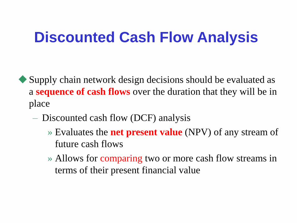
Discounted Cash Flow Analysis
Supply chain network design decisions should be evaluated as
a sequence of cash flows over the duration that they will be in
place
– Discounted cash flow (DCF) analysis
» Evaluates the net present value (NPV) of any stream of
future cash flows
» Allows for comparing two or more cash flow streams in
terms of their present financial value

Discounted Cash Flow Analysis
The present value of future cash is found by using a rate of return k
– A dollar today is worth more than a dollar tomorrow
– A dollar today can be invested and earn a rate of return k over the next period
Today… Tomorrow…
$1 $1*(1 + k)
$1/(1 + k) $1
Today… Tomorrow…
$1 $1*(1 + k)

6-5
Discounted Cash Flow Analysis
return of rate
flowscash of stream thisof luepresent vanet the
periods Tover flowscash of stream a is ,...,,
where
1
1
1
1factor Discount
10
1
0
k
NPV
CCC
Ck
CNPV
k
T
T
t
t
t
• Compare NPV of different supply chain design options
• The option with the highest NPV will provide the greatest
financial return

If… Then… So…
NPV > 0 Investment adds value
NPV < 0 Investment substracts value
NPV = 0 Investment would neither add
or substract value
Net Present Value
If… Then… So…
NPV > 0 Investment adds value The project may be accepted
NPV < 0 Investment substracts value The project should be rejected
NPV = 0 Investment would neither add
or substract value
Decision should be based on
other criteria

Example: Net Present Value
Trips Logistics can choose between two options
– Spot market rate expected at $1.20 per sq.ft. per year for
each of the next 3 years
– 3 year lease contract at $1 per sq.ft.

6-8
NPV Example: Trips Logistics
How much space to lease in the next three years
Demand = 100,000 units
Requires 1,000 sq. ft. of space for every 1,000 units of demand
Revenue = $1.22 per unit of demand
Decision is whether to sign a three-year lease or obtain warehousing space on the spot market
Three-year lease: cost = $1 per sq. ft.
Spot market: cost = $1.20 per sq. ft.
k = 0.1

NPV Example: Trips Logistics
Expected annual profit if space is obtained from spot
market using discount factor k = 0.1
Ct = (100,000 x $1.22) – (100,000 x $1.20)
= $2,000
C1
(1 + k)1
C2
(1 + k)2
C1
(1 + k)0NPV = + +
= $ 5,471
2,000
(1.1)1
2,000
1.12
2,000
(1.1)0= + +
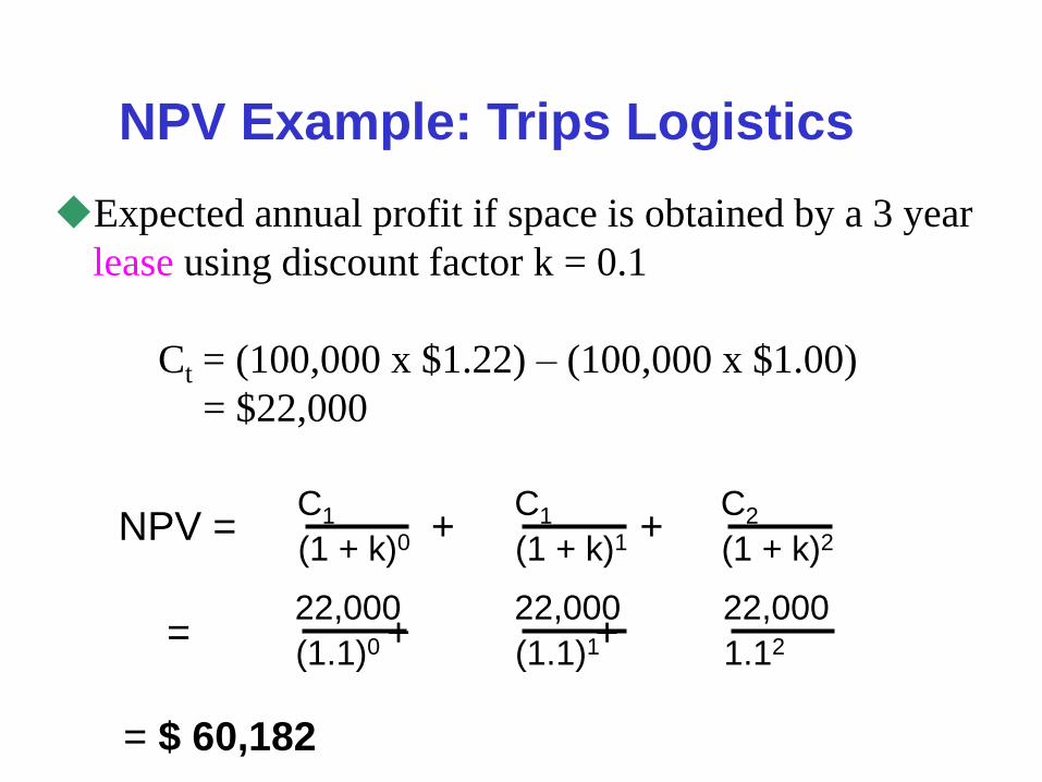
NPV Example: Trips Logistics
Expected annual profit if space is obtained by a 3 year
lease using discount factor k = 0.1
Ct = (100,000 x $1.22) – (100,000 x $1.00)
= $22,000
C1
(1 + k)1
C2
(1 + k)2
C1
(1 + k)0NPV = + +
= $ 60,182
22,000
(1.1)1
22,000
1.12
22,000
(1.1)0= + +
6-11
NPV Example: Trips Logistics
The NPV of signing the lease is $54,711 higher; therefore, the
manager decides to sign the lease
However, uncertainty in demand and costs may cause the
manager to rethink his decision

6-12
Representations of Uncertainty
Binomial Representation of Uncertainty
Other Representations of Uncertainty
6-13
Binomial Representations
of Uncertainty
When moving from one period to the next, the value of the
underlying factor (e.g., demand or price) has only two
possible outcomes – up or down
The underlying factor moves up by a factor or u > 1 with
probability p, or down by a factor d < 1 with probability 1-p
Assuming a price P in period 0, for the multiplicative
binomial, the possible outcomes for the next four periods:
– Period 1: Pu, Pd
– Period 2: Pu2, Pud, Pd2
– Period 3: Pu3, Pu2d, Pud2, Pd3
– Period 4: Pu4, Pu3d, Pu2d2, Pud3, Pd4

Binomial Representation of
Uncertainty
Pu3d2
Pu2d3
Pu4d
Pu5
Pud4
Pd5
Pu3d
Pu2d2
Pu4
Pud3
Pd4
Pu3
Pu2d
Pud2
Pd3
Pu2
Pud
Pd2
Pu
Pd
P
Multiplicative binomial
p
1-p
p
1-p
p
1-p
p
1-p
p
1-p
6-15
Binomial Representations
of Uncertainty
In general, for multiplicative binomial, period T has
all possible outcomes Putd(T-t), for t = 0,1,…,T
From state Puad(T-a) in period t, the price may move in
period t+1 to either
– Pua+1d(T-a) with probability p, or
– Puad(T-a)+1 with probability (1-p)

6-16
Binomial Representations
of Uncertainty
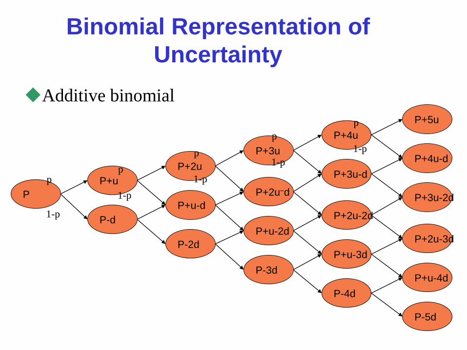
For the additive binomial, the states in the following
periods are:
– Period 1: P+u, P-d
– Period 2: P+2u, P+u-d, P-2d
– Period 3: P+3u, P+2u-d, P+u-2d, P-3d
– Period 4: P+4u, P+3u-d, P+2u-2d, P+u-3d, P-4d
In general, for the additive binomial, period T has all
possible outcomes P+tu-(T-t)d, for t=0, 1, …, T
Binomial Representation of
Uncertainty
P+3u-2d
P+2u-3d
P+4u-d
P+5u
P+u-4d
P-5d
P+3u-d
P+2u-2d
P+4u
P+u-3d
P-4d
P+3u
P+2u–d
P+u-2d
P-3d
P+2u
P+u-d
P-2d
P+u
P-d
P
Additive binomial
p
1-p
p
1-p
p
1-p
p
1-p
p
1-p
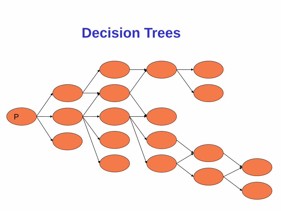
Decision Trees
P

Using Decision Trees
Can be used as visual aids to structure and solve sequential decision problems
Especially beneficial when the complexity of the problem grows

Decision Trees
Three types of “nodes”
– Decision nodes - represented by squares (□)
– Chance nodes - represented by circles (Ο)
– Terminal nodes - represented by triangles (optional)
Solving the tree involves pruning all but the best decisions at decision nodes, and finding expected values of all possible states of nature at chance nodes
Create the tree from left to right
Solve the tree from right to left

6-21
For each decision calculate the expected payoff as follows:
(The summation is calculated across all the states of nature)
Select the decision with the best expected payoff
Decision Trees

Example Decision Tree
Decision
node
Chance
node Event 1
Event 2
Event 3

Example of a Decision Tree
Problem
A glass factory specializing in crystal is experiencing a substantial
backlog, and the firm's management is considering three courses of
action:
A) Arrange for subcontracting,
B) Construct new facilities.
C) Do nothing (no change)
The correct choice depends largely upon demand, which may be low,
medium, or high. By consensus, management estimates the
respective demand probabilities as .10, .50, and .40.
© 2007 Pearson Education
Example of a Decision Tree Problem:
The Payoff Table
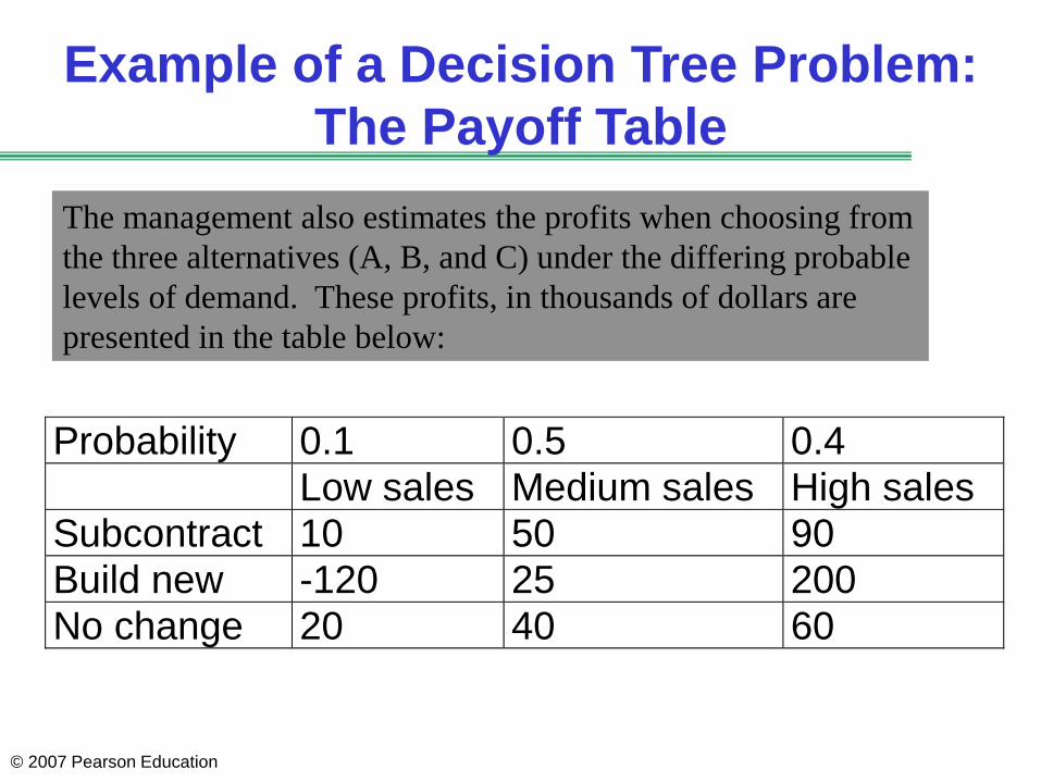
Probability 0.1 0.5 0.4
Low sales Medium sales High sales
Subcontract 10 50 90
Build new -120 25 200
No change 20 40 60
The management also estimates the profits when choosing from
the three alternatives (A, B, and C) under the differing probable
levels of demand. These profits, in thousands of dollars are
presented in the table below:

Example of a Decision Tree Problem:
Step 1. We start by drawing the three
decisions
Subcontract
Build New
No Change

Example of Decision Tree Problem:
Step 2. Add our possible states of
nature, probabilities, and payoffs
Subcontract
Build New
No Change
High demand (.4)
Medium demand (.5)
Low demand (.1)
$90k
$50k
$10k
High demand (.4)
Medium demand (.5)
Low demand (.1)
$200k
$25k
-$120k
High demand (.4)
Medium demand (.5)
Low demand (.1)
$60k
$40k
$20k

Example of Decision Tree
Problem: Step 3. Determine the
expected value of each decisionHigh demand (.4)
Medium demand (.5)
Low demand (.1)
Subcontract
$90k
$50k
$10k
EVA=.4(90)+.5(50)+.1(10)=$62k
$62k

Example of Decision Tree Problem:
Step 4. Make decisionHigh demand (.4)
Medium demand (.5)
Low demand (.1)
High demand (.4)
Medium demand (.5)
Low demand (.1)
A
B
CHigh demand (.4)
Medium demand (.5)
Low demand (.1)
$90k
$50k
$10k
$200k
$25k
-$120k
$60k
$40k
$20k
$62k
$80.5k
$46k
Alternative B generates the greatest expected profit, so our choice is
B or to construct a new facility.

6-29
Evaluating Network Design
Decisions Using Decision Trees
A manager must make many different decisions when
designing a supply chain network
Many of them involve a choice between a long-term (or less
flexible) option and a short-term (or more flexible) option
If uncertainty is ignored, the long-term option will almost
always be selected because it is typically cheaper
Such a decision can eventually hurt the firm, however,
because actual future prices or demand may be different
from what was forecasted at the time of the decision
A decision tree is a graphic device that can be used to
evaluate decisions under uncertainty

6-30
Decision Tree Methodology
1. Identify the duration of each period (month, quarter, etc.) and the number of periods T over which the decision is to be evaluated.
2. Identify factors such as demand, price, and exchange rate, whose fluctuation will be considered over the next T periods.
3. Identify representations of uncertainty for each factor; that is, determine what distribution to use to model the uncertainty.
4. Identify the periodic discount rate k for each period.
5. Represent the decision tree with defined states in each period, as well as the transition probabilities between states in successive periods.
6. Starting at period T, work back to period 0, identifying the optimal decision and the expected cash flows at each step. Expected cash flows at each state in a given period should be discounted back when included in the previous period.

6-31
Decision Tree Methodology Example:
Trips Logistics
Decide whether to lease warehouse space for the coming
three years and the quantity to lease
Long-term lease is currently cheaper than the spot market
rate
The manager anticipates uncertainty in demand and spot
prices over the next three years
Long-term lease is cheaper but could go unused if demand
is lower than forecast; future spot market rates could also
decrease
Spot market rates are currently high, and the spot market
would cost a lot if future demand is higher than expected

6-32
Trips Logistics: Two Options
Get all warehousing space from the spot market as
needed
Sign a three-year lease for a fixed amount of
warehouse space and get additional requirements from
the spot market

6-33
Trips Logistics
1 sq. ft. of warehouse space needed for 1 unit of demand
Current demand = 100,000 units per year
Binomial uncertainty: Demand can go up by 20% with
p = 0.5 or down by 20% with 1-p = 0.5
Lease price = $1.00 per sq. ft. per year
Spot market price = $1.20 per sq. ft. per year
Spot prices can go up by 10% with p = 0.5 or down by
10% with 1-p = 0.5
Revenue = $1.22 per unit of demand
k = 0.1

6-34
Trips Logistics Decision Tree
D=144
p=$1.45
D=144
p=$1.19
D=96
p=$1.45
D=144
p=$0.97
D=96
p=$1.19
D=96
p=$0.97
D=64
p=$1.45
D=64
p=$1.19
D=64
p=$0.97
D=120
p=$1.32
D=120
p=$1. 08
D=80
p=$1.32
D=80
p=$1.32
D=100
p=$1.20
0.25
0.25
0.25
0.25
0.250.25
0.25
0.25
Period 0
Period 1
Period 2

6-35
Trips Logistics Example
Analyze the option of not signing a lease and
obtaining all warehouse space from the spot market
Start with Period 2 and calculate the profit at each
node
For D=144, p=$1.45, in Period 2:
C(D=144, p=1.45,2) = 144,000x1.45 = $208,800
P(D=144, p =1.45,2) = 144,000x1.22 =$175,680
R(D=144,p=1.45,2) = 175,680-208,800 = -$33,120
Profit at other nodes are calculated similarly.

6-36
Trips Logistics Example
Expected profit at each node in Period 1 is the profit
during Period 1 plus the present value of the expected
profit in Period 2
Expected profit EP(D, p,1) at a node is the expected
profit over all four nodes in Period 2 that may result
from this node
PVEP(D=,p=,1) is the present value of this expected
profit and P(D=,p=,1), and the total expected profit, is
the sum of the profit in Period 1 and the present value
of the expected profit in Period 2

6-37
Trips Logistics Example
From node D=120, p=$1.32 in Period 1, there are four
possible states in Period 2
Evaluate the expected profit in Period 2 over all four states
possible from node D=120, p=$1.32 in Period 1 to be
EP(D=120,p=1.32,1) = 0.25xP(D=144,p=1.45,2) +
0.25xP(D=144,p=1.19,2) +
0.25xP(D=96,p=1.45,2) +
0.25xP(D=96,p=1.19,2)
= 0.25x(-33,120)+0.25x4,320+0.25x(-22,080)+0.25x2,880
= -$12,000

6-38
Trips Logistics Example
The present value of this expected value in Period 1 is
PVEP(D=12, p=1.32,1) = EP(D=120,p=1.32,1) / (1+k)
= -$12,000 / (1+0.1)
= -$10,909
The total expected profit P(D=120,p=1.32,1) at node D=120,p=1.32 in Period 1 is the sum of the profit in Period 1 at this node, plus the present value of future expected profits possible from this node
P(D=120,p=1.32,1) = [(120,000x1.22)-(120,000x1.32)] +
PVEP(D=120,p=1.32,1)
= -$12,000 + (-$10,909) = -$22,909
The total expected profit for the other nodes in Period 1 is calculated similarly

6-39
Trips Logistics Example
For Period 0, the total profit P(D=100,p=120,0) is the sum of
the profit in Period 0 and the present value of the expected
profit over the four nodes in Period 1
EP(D=100,p=1.20,0) = 0.25xP(D=120,p=1.32,1) +
= 0.25xP(D=120,p=1.08,1) +
= 0.25xP(D=96,p=1.32,1) +
= 0.25xP(D=96,p=1.08,1)
= 0.25x(-22,909)+0.25x32,073+0.25x(-15,273)+0.25x21,382
= $3,818
PVEP(D=100,p=1.20,0) = EP(D=100,p=1.20,0) / (1+k)
= $3,818 / (1 + 0.1) = $3,471

6-40
Trips Logistics Example
P(D=100,p=1.20,0) = 100,000x1.22-100,000x1.20 +
PVEP(D=100,p=1.20,0)
= $2,000 + $3,471 = $5,471
Therefore, the expected NPV of not signing the lease
and obtaining all warehouse space from the spot market
is given by NPV(Spot Market) = $5,471

6-41
Trips Logistics Example
Using the same approach for the lease option,
NPV(Lease) = $38,364
When uncertainty is ignored, the NPV for the lease
option is $60,182