Supply and Demand Shifts in the Shorting Market

LAUREN COHEN, KARL B. DIETHER, and CHRISTOPHER J. MALLOY∗

May 9, 2006

ABSTRACT

Using proprietary data on stock loan fees and quantities from a large institutional investor, we

examine the link between the shorting market and stock prices. Employing a unique identifi-

cation strategy, we isolate shifts in the supply and demand for shorting. We find that shorting

demand is an important predictor of future stock returns: An increase in shorting demand

leads to negative abnormal returns of 2.98% in the following month. Second, we show that

our results are stronger in environments with less public information flow, suggesting that the

shorting market is an important mechanism for private information revelation.

∗Cohen is at the Yale School of Management; Diether is at the Fisher College of Business, Ohio State Univer-sity; Malloy is at London Business School. We thank Viral Acharya, Nick Barberis, Ron Bird, Menachem Bren-ner, John Cochrane, Doug Diamond, James Dow, Darrell Duffie, Gene Fama, Ken French, Julian Franks, FranciscoGomes, Tyler Henry, David Hirshleifer, Kewei Hou, Charles Jones, Andrew Karolyi, Owen Lamont, Paul Marsh,Toby Moskowitz, Yigal Newman, Lubos Pastor, Jay Ritter, Jeanne Sinquefield, Rob Stambaugh, Jeremy Stein, RalphWalkling, Ingrid Werner, Karen Wruck, an anonymous referee, and seminar participants at the National Bureau ofEconomic Research, Western Finance Association, European Finance Association, Berkeley, University of Chicago,Harvard Business School, London Business School, Northwestern, Ohio State, Stanford, and Washington Universityfor helpful comments and suggestions. We also thank Gene Fama and Ken French for generously providing data.Please send correspondence to: Christopher Malloy, London Business School, Sussex Place, Regent’s Park, LondonNW1 4SA, UK, phone: 44-207-262-5050 x3278, email: cmalloy@london.edu.

An asset’s borrowing and lending market can have a large impact on its equilibrium price. For

stocks, an active borrowing and lending market exists,1 but its decentralized format and lack of

transparency make isolating a direct link to stock prices difficult. The standard empirical approach

to testing the relation between the shorting market and future returns relies on either 1) obtaining

data on the direct costs of shorting from the stock loan market, as such costs provide a measure of

the constraints on short selling,2 or 2) employing proxies for shorting demand or shorting supply.

The idea behind looking at shorting demand is that some investors may want to short a stock but

may be impeded by constraints; if one can measure the size of this group of investors, then one

can measure the extent of overpricing or the extent of private information left out of the market.

The idea behind looking at shorting supply is that shorting a stock requires that one first borrow

the shares, and thus a low supply of lendable shares may indicate that short sale constraints are

binding tightly.

In this paper, we provide a new framework for testing how stock prices respond to activity

in the shorting market. Our approach allows us to construct actual measures of shorting supply

and shorting demand. We argue that decomposing the competing effects of shorting supply and

shorting demand is a crucial and overlooked aspect of the empirical literature on short selling, as

it enables one to explicitly test which theoretical channel drives the relation between the shorting

market and future returns.

Using a novel four-year panel data set consisting of actual loan prices and quantities from a

large institutional investor, we employ an empirical strategy that allows us to isolate supply and

demand shifts in the equity lending market. Instead of taking a component of the intersection of

supply and demand and using it to proxy for demand or supply (thereby assuming the opposite

curve is inelastic, or does not shift), as is common in the literature, we attempt to disentangle these

two effects. We are able to infer if a stock has experienced an increase or decrease in shorting

demand or shorting supply by exploiting price-quantity “pairs.” For example, an increase in the

loan fee (our measure of price) coupled with an increase in the percentage of outstanding shares

on loan (our measure of quantity) corresponds to at least an increase in shorting demand, as would

be the case for any increase in price coupled with an increase in quantity. We do not maintain that

this is the only shift that occurred. However, for a shift of price and quantity into this quadrant, at

least a demand shift outward must have occurred. By classifying shifts in this way, we are able to

1

identify shifts in shorting demand and supply, and then explore the effect of these shifts on future

stock returns.

Differentiating supply and demand is crucial for determining the channel through which, and

thus the reason why, stock prices respond to activity in the shorting market. Mechanically, if

shorting demand is the dominant channel, then the coupling of both increased (decreased) price

(i.e., loan fee) and increased (decreased) quantity (i.e., short interest, or percentage of shares on

loan) are important. Increased quantity, for instance, could be informative for future stock returns

if it proxies for additional market frictions or risks of shorting, or if it signals a higher probability of

informed trading. For example, if short-selling capital is limited, then taking a large short position

in a stock potentially subjects a short-seller to idiosyncratic risk that she cannot diversify away.

Nonprice marginal costs of shorting such as recall risk may also be increasing in quantity.3 Either

way, large short positions may require a risk premium. Alternatively, as in Diamond and Verrecchia

(1987), high unexpected short interest may signal a large quantity of negative private information,

since fewer liquidity traders (or those shorting for hedging purposes) are likely to short in the face

of high short selling costs. Overall, changes in shorting demand represent changes in the marginal

benefits of investors. If shorting demand is important empirically, then private information or other

indirect costs/risks of shorting are key factors in the link between the shorting market and stock

prices.

The factors driving changes in shorting supply are different. Supply shifts are driven by

changes in institutions’ marginal cost of lending. For instance, because many lending institu-

tions (including ours) also operate mutual funds, they have other incentives for holding stocks.

Following a sale of the shares of a certain stock in its funds, a lending institution experiences an

inward shift of its supply curve for the stock.4 However, any movement in marginal costs will

shift this curve. The interpretation and implications of shifts driven by contractions of shorting

supply are therefore quite different from those of shifts driven by increases in shorting demand.

Supply shifts inward (outward) indicate tightening (loosening) of short sale constraints, while de-

mand shifts capture either informed trading or the additional market frictions and risks associated

with shorting. Thus, isolating the relative effects of supply and demand empirically is crucial for

developing a better understanding of the impact of the shorting market on stock prices.

Our tests reveal that shorting demand is an economically and statistically significant predictor

2

of future stock returns. Our pooled, cross-sectional regression estimates indicate that an increase in

shorting demand leads to a significant negative average abnormal return of 2.98% in the following

month. Decreases in shorting supply play a more minor role. We also find that the loan fee is not

a sufficient statistic for overpricing, as proposed in the previous literature. Rather, “specialness”

(i.e., a high loan fee) is only important for future returns when driven by increases in shorting

demand.

Turning to the issue of interpretation, we investigate whether increased shorting demand signals

informed trading (which then leaks out to the market and reduces prices), or whether it proxies for

additional market frictions (which lead to higher expected returns for shorting, net of loan fees). To

explore private information we exploit variation in the public information environment, and relate

this to variation in the strength of the shorting market’s ability to predict future returns. We then

examine the implications of private information flow as an important mechanism in this market,

relative to costs. Specifically, we examine the costs and benefits in terms of returns to a demand

shift-based trading strategy, net of the explicit cost of shorting. While in general we would not

expect to find substantial profits net of trading costs unless the indirect costs or risks of shorting are

extremely large, if the lending market is an important channel for private information revelation,

then substantial profits net of trading costs would not be unreasonable. Lastly, we explore the

extent to which additional indirect costs and risks of shorting (e.g., recall risk or arbitrage risk) can

explain the predictive ability of shorting demand.

We show that our key results are unlikely to be driven by public information flow. The effect

of shorting demand on future stock returns is not concentrated among stocks with high analyst

coverage (a proxy for public information flow), nor is it driven by predictable shifts in shorting

demand due to dividend capture borrowing. We also estimate the return to an investor who uses our

identification strategy to form trading rules. Net of shorting costs, on average the investor makes

over 47% per year. Even after incorporating trading costs such as commissions, bid-ask spreads,

and price impact, a conservative estimate of the average return performance of the strategy still

yields 4.5% per year. The Sharpe ratio of the strategy is about 2.5 to 3.5 times that of the market

or HML. Thus, the indirect costs of shorting would have to be extremely large, or arbitrage capital

would have to be very limited for this strategy to represent a risk premium earned by short-sellers.

However, we find little evidence that the profits to the shorting demand strategy vary with proxies

3

for recall risk or stock-level arbitrage risk. Overall, our results indicate that the shorting market is

an important mechanism for private information revelation.

The paper remainder of the paper is organized as follows. Section I reviews the related litera-

ture. Section II describes our research design and the data used in the study. Sections III and IV

present empirical results, and Section V concludes.

I. Related Literature

A large literature explores the theoretical link between short sale constraints and asset prices.5

Miller (1977) posits that the combination of differences of opinion and short sale constraints can

lead to overpricing. Differences of opinion can arise from overconfidence (Scheinkman and Xiong

(2003)) or from differences in prior beliefs which are updated rationally as information arrives

(Morris (1996)). In this setting, stock prices reflect the views of optimists, and this pattern of

overpricing leads to low subsequent returns.6 Diamond and Verrecchia (1987), in contrast, argue

that rational uninformed agents take the presence of short sale constraints into account when form-

ing their valuations, and thus that there is no overpricing conditional on public information as all

participants recognize that negative opinions have not made their way into the order flow. Dia-

mond and Verrecchia’s (1987) common-priors rational expectations model does predict, however,

that short sale constraints impede the flow of private information, and that the release of negative

private information (e.g., via an unexpected increase in short interest) leads to negative returns.

The effect of short sale constraints on stock prices is ultimately an empirical question. One

key empirical issue is determining an appropriate measure of short sale constraints. Due to the

difficulty of obtaining data on direct shorting costs, a variety of studies exploit the fact that an

unwillingness or inability to short may limit the revelation of negative opinions in the same way as

shorting costs. For example, institutional or cultural norms may limit shorting. Almazan, Brown,

Carlson, and Chapman (2000) find that only about 30% of mutual funds are allowed by their

charters to sell short and only 2% actually do sell short. Chen, Hong and Stein (2002) use this

fact to motivate their choice of breadth of mutual fund ownership as an indicator of the extent to

which negative valuations are not expressed in prices. They find that reductions in breadth, which

signal an increase in the amount of negative information withheld from the market, lead to negative

subsequent abnormal returns on average during the sample period, 1979 to 1998. Similarly, Nagel

4

(2005) uses residual institutional ownership as a proxy for shorting demand (again assuming low

residual institutional ownership signals that negative information is being withheld from stock

prices) and finds that underperformance in growth stocks and high dispersion stocks is concentrated

among stocks with low institutional ownership. However, Nagel (2005) also finds that when he

combines his sample period with that in Chen, Hong, and Stein (2002) period, there is no longer

a reliable pattern during the 1980 to 2003 period between breadth of mutual fund ownership and

future returns. Residual institutional ownership may also proxy for shorting supply, since low

institutional ownership restricts the supply of available shares on loan. As in Chen, Hong, and

Stein (2002), it is not clear which channel (shorting demand or shorting supply) drives the results.

Mutual fund and institutional investment, aside from representing only a portion of the investing

universe, are also driven by nonshorting considerations such as investment style.

The oldest strand of the empirical literature on short-selling focuses on short interest ratios

(shares sold short divided by shares outstanding) as a proxy for shorting demand. Many of the

early empirical studies (see Desai, Ramesh, Thiagarajan, and Balachandran (2002) for a summary)

fail to find a consistent relation between short interest and abnormal returns. This could be due

to the problematic nature of short interest. For example, a low level of short interest may not

indicate low shorting demand: Stocks that are impossible to short could have a huge shorting

demand, yet the level of short interest is zero. The weak results could also be due to the typical

focus on levels of short interest, rather than changes.7 Alternatively, Desai, Ramesh, Thiagarajan,

and Balachandran (2002) argue that the weak results could be due to the use of small and/or

biased samples in these early studies. Indeed, much of the modern empirical literature linking

the level of short sales with future returns finds consistent evidence that high short interest is

followed by low future returns. For example, Asquith and Meulbroek (1995) and Desai, Ramesh,

Thiagarajan, and Balachandran (2002) find significant abnormal returns for stocks with high short

interest on, respectively, the NYSE and Nasdaq exchanges for 1976 to 1993 and 1988 to 1994.8

Boehme, Danielsen, and Sorescu (2006) and Mohanaraman (2003) combine high short interest

with measures of differences of opinion (the standard deviation of residuals and dispersion in

analysts’ forecasts, respectively) to test the Miller (1977) story; Boehme, Danielsen, and Sorescu

(2006) find that the underperformance of stocks with high short interest ratios is concentrated

among small stocks with high residual standard deviation, and Mohanaraman (2003) finds that high

5

short interest stocks have lower returns the greater the dispersion in analysts’ forecasts. Finally,

Aitken, Frino, McCorry, and Swan (1998), Angel, Christophe, and Ferri (2003), and Diether, Lee,

and Werner (2006) look at daily short sales and subsequent returns and find that high daily short

sales are followed quickly by negative abnormal returns.

Asquith, Pathak, and Ritter (2005), one of the few papers that explicitly recognizes the compet-

ing effects of shorting supply and shorting demand, argue that stocks with high shorting demand

and low shorting supply are the most likely to face binding short sale constraints. They show that

stocks in the highest percentile of short interest (their proxy for shorting demand) and the lowest

third of institutional ownership (their proxy for shorting supply) underperform by 215 basis points

per month during the 1988 to 2002 period on an equal-weight basis. However, they do not attempt

to disentangle the individual effects of shorting supply and shorting demand, and their focus is on

levels (rather than changes); since they proxy for shorting supply and demand using institutional

ownership and short interest, they also face the same interpretation problems mentioned above.

Our paper is unique in that we are able to use actual data on loan fees and loan amounts (not prox-

ies) to decompose the effect on stock prices into the part that is due to shorting demand, and the

part that is due to shorting supply.

A series of recent papers analyzes direct measures of shorting costs (price).9 The most com-

monly used metric is the rebate rate, in particular, the spread between the rebate rate and the market

interest rate. The rebate rate is the fee that the lender of the stock must pay back to the borrower

of that stock. This fee arises because in order to sell a stock short, an investor must borrow shares

from an investor who owns them and is willing to lend them. The short-seller must leave collateral

with the lender in order to borrow the shares; in turn, the lender pays the short-seller interest - the

“rebate” rate - on this collateral. Retail borrowers typically receive no interest on their proceeds, so

the situation described above applies mainly to institutional short-sellers. The difference or spread

between the interest rate on cash funds and the rebate rate is a direct cost to the short-seller, and

is often referred to as the loan fee. The rebate rate serves to equilibrate supply and demand in the

stock lending market, much like the “repo” rate in the fixed income market.10 Obviously, if every

investor were willing and able to lend shares in a competitive market, the lending fee would be

close to zero. But, as Duffie (1996) and Krishnamurthy (2002) show, if some investors willing to

hold overpriced assets do not lend, a strictly positive fee can arise.

6

The existing evidence on rebate rates has generally been limited to proprietary databases over

short time periods. Using a database from a single lender from April 2000 through September

2001, D’Avolio (2002) reports that only 9% of the stocks in his sample are “on special” (defined

here as a loan fee greater than 1% per annum) on a typical day. The other 91% typically have

loan fees around 20 basis points per annum. In other words, the rebate rate is typically about

20 basis points less than the Federal Funds rate. He does find that stocks on special have higher

short interest. Using a sample of rebate rates from a single lender from November 1998 through

October 1999, Geczy, Musto, and Reed (2002) conclude that short sale constraints are unable to

explain anomalous patterns in stock returns. Meanwhile, using proprietary data from July 1999 to

December 2001, Ofek, Richardson, and Whitelaw (2004) document that stocks on special are more

likely to violate put-call parity.11 Finally, using a small database of rebate rates hand-collected

from the Wall Street Journal from 1926 to 1933, Jones and Lamont (2002) find that stocks with

low rebate rates (high loan fees) experience low subsequent returns. However, the effect is modest;

the authors only find large negative size-adjusted returns (−2.52% in the following month) among

stocks that are both expensive to short and new to the loan crowd (another proxy for high shorting

demand).

Virtually all existing papers also fail to address the exact mechanism that causes the observed

movement in stock prices. However, the problem of causation is mitigated in a few papers. For

example, Sorescu (2000) looks at options introductions, while Ofek and Richardson (2003) look at

lockup expirations; lockup expirations, in particular, are exogenous events that might reduce short

sale constraints. Both papers find significant negative abnormal returns following these events.

However, both of these papers again use proxies for shorting demand or shorting supply, and

both focus on selected samples of stocks. Sorescu (2000) only analyzes optionable stocks, which

tend to be large, while Ofek and Richardson (2003) only explores Internet IPOs. In addition,

Mayhew Mihov (2005) find no evidence that investors take disproportionately bearish positions

in newly listed options. This may serve to weaken the causal link between a relaxation of short

sale constraints and stock prices in the context of option introductions. In this paper, we focus on

the entire universe of small stocks (where shorting costs should be most relevant) and attempt to

address the endogeneity of shorting indicators explicitly.

7

II. Research Design

A. Data

We use a proprietary database of stock lending activity from a large institutional investor. This

institution - unnamed for confidentiality purposes - is a market maker in many small stock lending

markets. The data include daily contract-level data on rebate rates, the number shares on loan, col-

lateral amounts, collateral/market rates, estimated income from each loan, and broker firm names

for the entire universe of this firm’s lending activity from September 1999 to August 2003.

The rebate rate is the portion of the collateral account interest rate that the short-seller receives

back.12 For each observation, we compute the loan fee, which is equal to the interest rate on cash

funds (known as the “market rate” or “collateral rate”) minus the rebate rate. Variation in the rebate

rate therefore determines the cross-sectional variation in the loan fee, and hence the direct cost to

the short-seller of maintaining the short position. The loan fee is our measure of price throughout

the paper. While each stock may have multiple lending contracts on a given day, the loan fees

are almost always very similar. We use the loan fee of the largest contract in our tests, but our

results are unaffected by using the average or share-weighted average loan fee instead. Throughout

the paper we use the number shares on loan divided by the number of shares outstanding as our

measure of quantity in order to use a consistent measure across stocks; however, untabulated results

indicate that our key findings are slightly stronger if we use raw, unscaled shares on loan as our

measure of quantity instead.

Panel A of Table I presents lending activity examples from our sample. A typical large stock

such as Intel has a very small loan fee (0.05% per year), and our lending institution lends out only

a fraction of the total shares outstanding. By contrast, for a small stock, such as Atlas Air, the loan

fee can be very high (7.25% per year), and our institution may lend out a large share (almost 5%)

of the total shares outstanding. Our lender is a large presence in the small cap market, owning 5%

or more in over 600 small cap stocks throughout the sample period, and owning at least a small

stake in the vast majority of stocks below the NYSE median market cap. Further, it is more active

in the small stock lending market, making an average of 11.79 loans per stock per day across all

small cap stocks as opposed to 4.64 for large stocks.

Insert Table I About Here

8

Untabulated statistics indicate that our lender accounts for a substantial fraction of overall

market lending in small cap securities. For example, among stocks below (above) the NYSE

median market capitalization that are also on loan by our lender, the average ratio of our fund’s

percentage on loan to the total short interest is 26% (2%); in 13.6% of the observations the fund

is responsible for at least 67% of the short interest, and in 7.5% of the observations the fund is

responsible for all of the short interest. On the other hand, our lending institution seems to be a

relatively less important lender in the large cap lending market.

We merge our lending data with information from a variety of other sources. We draw data on

stock returns, shares outstanding, volume, and other items from CRSP, book equity from COM-

PUSTAT, monthly short interest data from Nasdaq, analyst coverage from I/B/E/S, and quarterly

institutional holdings from CDA/Spectrum.

Panel B of Table I presents summary statistics for our main sample, broken down into large

stocks (stocks above the NYSE median market cap) and small stocks (stocks below the NYSE

median market cap). We restrict our sample to stocks with lagged (t − 1) price greater than or

equal to $5. First, this ensure that our results are not driven by small, illiquid stocks. In addition,

collateral requirements have a nonlinearity below prices of $5 for our lender, which may distort

lending preferences and rebate rates. Low priced stocks are also more likely to go bankrupt, and

in the case of bankruptcy a short-seller may have to wait months to recover the collateral funds.

Clearly, small stocks have much higher loan fees on average (Loan Fee = 3.94% per annum, versus

0.39% for large stocks), and our institution lends out much larger shares of these small stocks

(0.85% of shares outstanding on average, versus 0.14% for large stocks). The market (or collateral)

interest rate in Panel B for stocks above the NYSE median is more than 160 basis points less than

the market rate for stocks below the NYSE median, but this result is simply due to the calendar

timing of these two samples. Our institution dramatically increased its large-cap (above NYSE

median) lending program in 2002 and 2003, while maintaining its small-cap (below NYSE median)

lending program at a relatively constant level throughout our sample period. For example, the

average number of stocks on loan per day for a given calendar year is 366, 438, 320, and 317 over

the 2000 to 2003 period for small-cap stocks, compared to 20, 68, 249, and 350 over the same

period for large-cap stocks. Therefore, the large-cap sample is concentrated at end of the sample

period, when market interest rates were lower. To avoid this calendar clustering in our sample, to

9

focus our analysis on the area in which short sale constraints are presumably most important, and

to mitigate the substitution problem noted below, our tests examine only stocks below the NYSE

median market capitalization.

B. Price and Quantity “Pairs”

Our primary goal is to evaluate the effect of shifts in the supply and demand for shorting on

future stock returns. To do so, we must first isolate clear shifts in the supply and demand for

shorting. Our identification strategy consists of constructing price-quantity “pairs” using our data

from the equity lending market. For example, an increase in the stock loan fee (i.e., price) coupled

with an increase in the percentage of shares on loan (i.e., quantity) corresponds to an increase

in shorting demand, as would be the case for any increase in price coupled with an increase in

quantity. As noted earlier, we do not insist that this is the only shift that occurred. However, for a

shift of price and quantity into this quadrant, a demand shift outwards must have occurred. A key

point to understand is that these price-quantity shifts correspond to movements in a stock’s loan

price and loan quantity, not its actual share price or number of shares outstanding.

We classify movements in loan prices and quantities by placing stocks into one of four quad-

rants at each point in time: Those that have experienced at least a demand shift out (DOUT ), at

least a demand shift in (DIN), at least a supply shift out (SOUT ), and at least a supply shift in

(SIN). More precisely, stocks in DOUT have seen both their loan fee and their loan amount rise

(over the designated horizon), stocks in DIN have seen both their loan fee and loan quantity fall,

stocks in SOUT have seen their loan fee fall but their loan quantity rise, and stocks in SIN have

seen their loan fee rise but their loan quantity fall.13 Thus, our classification scheme allows us

to infer whether the stock has experienced an increase or decrease in the supply or demand for

shorting over the chosen horizon.

This simple approach raises a number of obvious questions. First, the horizon over which these

shifts is measured may b potentially crucial. For instance, one could observe an increase in the loan

fee followed by a decrease in the loan fee, but over some horizon the net change might be zero.

We therefore experiment over a variety of possible horizons. Second, by placing a stock into only

one of the four quadrants at any point in time, we are restricting our attention to cases in which

there is “at least” a shift of the type described. Clearly, a stock placed in the DOUT quadrant may

10

also have experienced an increase in shorting supply over the designated period. While both shifts

imply an increase in the quantity on loan, only DOUT implies an increase in the loan fee. Thus, if

we observe an increase in quantity and fee, irrespective of all other shifts, we know that at least a

demand shift out has occurred. It is in this sense that we refer to each of our quadrants as signifying

“at least” a shift of a given type.

C. Testable Hypotheses

Our shifts allow us to test a variety of hypotheses about the relation between the shorting

market and future stock returns. The first important factor in forming testable hypotheses is a

careful consideration of the timing involved. In a rational expectations framework like Diamond

and Verrecchia (1987), it is reasonable to expect that prices will incorporate negative private infor-

mation fairly quickly. By contrast, while the empirical literature on overpricing largely abstracts

from the issue of timing, several papers seem to argue that overpricing is a long-run phenomenon

that is corrected slowly over a series of months and quarters (rather than days or weeks). For

example, Chen, Hong, and Stein (2002) use changes in breadth of mutual fund ownership to

forecast returns up to four quarters in the future, and Lamont (2004) looks at returns one to three

years after firms’ battles with short-sellers. Of course, there is no theoretical reason why this

should be the case, and since we have no clear priors regarding what exactly is the “short-run”

versus the “long-run,” our preferred approach is to let the data speak for itself. In our data, the

median stock lending contract is held for around three weeks. Thus, to mirror this fact we use

one-month holding periods for most of the tests in the paper. In Section III.B we examine shorter

and longer horizons as well.

HYPOTHESIS 1: DOUT predicts negative future returns.

DOUT captures the case in which both the cost of shorting (i.e., loan fee) and the amount

that investors are willing to short at this higher cost increase. Effectively, more capital is betting

that the price will decrease, despite the higher explicit cost of betting. DOUT may signal a

large quantity of negative private information, since fewer liquidity traders (or those shorting

for hedging purposes) are likely to short in the face of high short selling costs (Diamond and

Verrecchia (1987)).14 Alternatively, DOUT may capture additional costs or risks of shorting. For

11

example, if short-selling capital is limited, then taking a large short position in a stock potentially

subjects a short-seller to idiosyncratic risk that she cannot diversify away. Nonprice marginal costs

of shorting such as recall risk may then be increasing in quantity. In both views, DOUT predicts

negative returns.

HYPOTHESIS 2: DIN predicts positive future returns.

DIN captures the case in which both shorting costs and the amount that investors borrow

at this lower price decrease. DIN predicts positive future returns: Even though shorting costs

decrease, investors are willing to allocate less capital to shorting. We expect this to be a weak

predictor of positive future returns, however. If investors have positive opinions or information

about the company, they could express this more directly (and often in a much less costly way) by

actually purchasing the stock. Contrast this with the expected effect of DOUT . Because options

do not exist for most of the stocks in our sample, shorting is the only way to bet on a downturn in

the security price. We therefore expect DOUT to be a stronger predictor of future returns than DIN.

HYPOTHESIS 3: SIN predicts positive future returns, as tightening the constraint allows

additional overpricing.

We postulate that decreases in shorting supply (SIN) indicate tightening of short sale con-

straints, and increases in shorting supply (SOUT ) indicate relaxing of short sale constraints. SIN

indicates an increase in the cost of shorting coupled with a decrease in the amount that investors

are willing to short at this higher price. With less shares being shorted at a higher cost, the

constriction in the supply of lendable shares represents a tightening of the constraint on shorting.

Facing this higher cost, investor capital leaves the shorting market, which leads stocks to become

more overpriced. Note that this conjecture contrasts with Chen, Hong, and Stein (2002), who

argue that decreases in breadth of ownership (i.e., the tightening of short sale constraints) should

lead to low returns. However, their focus is on the eventual correction of long-run overpricing,

while our focus is on the short-run effects of increased overpricing.

HYPOTHESIS 4: SOUT predicts negative future returns: The constraint on previously overpriced

securities relaxes, and their prices converge back to fundamental value.

12

By contrast, SOUT indicates a decline in the cost of shorting coupled with an increase in the

amount investors are willing to borrow at this lower rate. Because the lowering of the cost makes

it possible for more investors to enter the market, increased shorting at this lower price signals

that there may have been a constraint relaxation. Note that if this relaxation leads to an immedi-

ate downward price adjustment, then SOUT will be a weaker signal then DOUT for predicting

subsequent returns since some of the mispricing may be mitigated immediately.15

D. Shift Characteristics

Summary statistics of the effect of each type of shift on both loan fee (price) and the quantity

on loan are presented in Table II. The average change in loan fee from each of the shifts is roughly

40 basis points, except for SOUT , which results in a 56 basis point decrease on average. The

average change in shares on loan as a percentage of shares outstanding following each shift is

approximately 0.30%. The number of stocks that experience a particular shift in a given month can

be small in some months. For example, on average the number of stocks per month that experience

at least an outward demand shift (DOUT ) is 22 (median=14). For this reason, we perform a variety

of robustness checks below that are designed to analyze the extent to which our results are sample

specific.

Insert Table II About Here

One potential caveat with regard to our shift measures is that because we only have one lender,

we might capture substitution across lenders within a security instead of actual increases in supply

or demand. For example, if an investor moves her lending activity from Institution A to our insti-

tution, we may measure this as a demand shift out, when in fact there has been no increase in the

shorting demand for this stock. We employ a number of tests to address this issue, all of which

indicate that this caveat is unlikely to affect our results.

First, as noted in Section II.A, our lender comprises a substantial fraction of overall market

lending for small cap stocks, making up on average 26% (but up to all) of the total short interest

for the stocks on loan by the institution that are below the NYSE median market cap. Second,

as described below, we run additional tests that attempt to exploit variation in our lender’s mar-

ket share. For example, we run regressions that interact the shift variables with the percentage of

13

aggregate short interest that our institution is lending out. We find that the shift results are signif-

icantly stronger for stocks in which our institution lends out a substantial fraction. We also use

aggregate short interest as a measure of quantity (in place of the amount lent out by our lender),

since substitution is obviously not an issue using aggregate short interest. Again, our results are

robust to this alternate specification. However, in light of practitioners’ claims that monthly short

interest is subject to window dressing (see D’Avolio (2002)) and is only a single snapshot in time,

we prefer to use the daily lending quantities from our institution in our baseline tests.

E. Cross-Sectional Regressions

Our baseline tests employ pooled, cross-sectional regressions on the universe of securities be-

low the NYSE median market capitalization breakpoint to determine the effect of the shift vari-

ables in predicting future returns. To control for the well-known effects of size (Banz (1981)),

book-to-market (Rosenburg. Reid, and Lanstein (1985), Fama and French (1992), and momentum

(Jegadeesh and Titman (1993), Carhart (1997)), we characteristically adjust the left-hand side re-

turns (as in Grinblatt and Moskowitz (1999)) for size and book-to-market using 25 equal-weight

size/book-to-market benchmark portfolios and we control for past returns on the right-hand side.16

Specifically, we regress the cross-section of characteristically-adjusted individual stock returns

at time t on a constant, DIN, DOUT , SIN, SOUT , r−1 (last month’s/week’s return), r−12,−2 (the

return from month t−12 to t−2), r−52,−2 (the return from week t−52 to t−2), IO (institutional

ownership, measured as a fraction of shares outstanding lagged one quarter), volume (the aver-

age daily exchange-adjusted share turnover during the previous six months), Loan Fee, Quantity,

∆(Loan Fee), and ∆(Quantity). We compute our four variables of interest (DIN, DOUT , SIN,

and SOUT ) as follows. The last trading day of month (week) t − 1 we check if there was some

kind of shift in supply or demand during the month (based on changes in loan fees and shares on

loan). We define DIN as a dummy variable equal to one if the stock experienced an inward demand

shift last month (or week, depending on the horizon of the left-hand side returns); DOUT , SIN,

and SOUT are defined analogously for outward demand shifts, inward supply shifts, and outward

supply shifts, respectively. We include last month’s (week’s) return to control for reversals, and

the prior year’s return to control for the momentum effect. We include institutional ownership to

control for how widely held the security is by the most probable security lenders (institutions).

14

In addition, we include trading volume, as it may proxy for a number of effects including liquid-

ity, recall risk, or general disagreement among investors about a firm’s price (Miller (1977)). The

variable Loan Fee is a continuous variable measuring the spread between the market rate and re-

bate rate, Quantity equals the end-of-month/week ratio of shares on loan by our institution to total

shares outstanding, ∆(Loan Fee) is the change in loan fee over the past month, and ∆(Quantity) is

the change in the fraction of shares on loan by the lender over the past month.

The baseline model takes the form

r j,t −RSB j,t−1t = αt +β1DIN j,t−1 +β2DOUTj,t−1 +β3SIN j,t−1 +β4SOUTj,t−1+ (1)

β5r j,t−1 +β6r j,t−12,−2 +β7IO j,t−3 +β8Volume j,t−7,−1 + ε j,t ,

where r j,t is the return on security j and RSB j,t−1t is the return on the size/book-to-market-matched

portfolio.

The regressions include calendar month dummies, and the standard errors take into account

clustering by month employing a robust cluster variance estimator. Note that we run these re-

gressions using a Fama and MacBeth (1973) approach as well, and the results are very similar.

We prefer the pooled approach because some of the time periods used in the Fama and MacBeth

(1973) regressions contain few observations that experienced a particular shift.

III. Empirical Results

A. Monthly Return Regressions

The cross-sectional regression estimates in Table III indicate that increases in the demand for

shorting (DOUT ) lead to large negative abnormal returns in the future. Column two of Table III

indicates that even after characteristically adjusting for size and book-to-market and controlling

for past returns, institutional ownership, and volume on the right-hand side of these regressions,

average abnormal returns for stocks experiencing an outward shift in shorting demand are -2.98%

in the following month (t=-3.96). We also see from column 2 that both institutional ownership,

which proxies for ease of shorting a stock, and volume, which could proxy for a number of effects

including recall risk, disagreement, and liquidity, do not significantly affect abnormal returns after

controlling for the shifts.

15

Insert Table III About Here

Table III indicates that DOUT shifts consistently exhibit large predictive ability for future

stock returns. By contrast, the other shifts have less predictive ability, despite the fact that the

average magnitude of each of the shifts themselves in terms of loan fee and quantity (from Table

II) is roughly equivalent; DOUT shifts are actually the least common in frequency. For example,

column 2 shows that average abnormal returns for stocks experiencing an outward shift in shorting

supply (SOUT ) are -0.63% in the following month (t=0.91). Decreases in shorting demand (DIN)

and decreases in shorting supply (SIN) lead to positive, but insignificant abnormal returns in the

future (0.50% and 0.35% per month, respectively). Overall, our results suggest an economically

and statistically important link between increases in shorting demand (DOUT ) and future abnormal

returns, but almost no link between SOUT , SIN, DIN and future abnormal returns.

To highlight the importance of our shift classification strategy, we examine the predictability

of different specifications that include quantity levels, loan fee levels, quantity changes, and loan

fee changes. The effects of loan fees (Loan Fee) and quantities (Quantity) are displayed in regres-

sions 3 to 7 in Table III. Consistent with a number of recent papers (Jones and Lamont (2002),

Reed (2002), and Geczy, Musto, and Reed (2002)), we find that high shorting costs, specifically

Loan Fee > 5% per annum, predict future negative returns. However, when we include the shift

variables in column 7, the conditional effect of these high costs is no longer significant, while

DOUT remains large and significant (-2.36%, t=3.27).17 The quantity level is uninformative; as

shown in columns 4 and 6, the marginal effect of the interaction of quantity level with high loan

fees (either Loan Fee > 300 or Loan Fee > 500) is insignificant. Lastly, we examine the effects of

quantity changes and loan fee changes separately, since quantity can increase because of either a

supply shift out or a demand shift out (and decrease because of a supply shift in or a demand shift

in), while the loan fee can increase because of an supply shift in or a demand shift out (and decrease

because of a supply shift out or a demand shift in). We compute quantity changes (∆Quantity) and

loan fee changes (∆Fee) at month t− 1, and test their predictive ability for next-month returns in

columns 8 and 9 of Table III. Column 8 indicates that returns are negative following loan fee in-

creases and quantity increases, and significant for ∆Quantity, although the magnitudes are smaller

than for the shift portfolios. Again, however, when the shift portfolios are included, the conditional

16

effect of ∆Quantity decreases. Also, DOUT remains negative and highly significant (-2.49%, t=-

3.19). In fact, our results suggest that quantity and loan fee increases may be noisy proxies for a

portion of DOUT . Using the raw number of shares on loan as our measure of quantity (rather than

dividing shares on loan by shares outstanding for each firm) changes none of our conclusions: The

effect of DOUT is still large (-2.23%, t=2.52), and the conditional effect of ∆(Quantity) is still

insignificant. The results in Table III highlight the ability to make richer empirical predictions of

future returns by using the shift portfolio classification.

B. Speed of Price Adjustment

An important issue in analyzing the effect of shifts in shorting supply and shorting demand on

future stock returns is measuring the speed with which prices change. Our previous results indicate

that increases in shorting demand at the monthly frequency lead to significantly lower returns in

the following month. By contrast, shifts in shorting supply and decreases in shorting demand have

weaker effects on future returns at the monthly horizon. However, it is possible that these shifts

may affect prices at even higher frequencies, or that changes in shorting supply may change prices

more quickly than changes in shorting demand.

To explore the stock price dynamics in greater depth, we perform a variety of tests. First, we

replicate all of our monthly regressions at the weekly level. These weekly estimates (unreported,

but available on request) reveal a similarly strong relation between abnormal returns and increases

in shorting demand, and similarly weak relations between abnormal returns and the other three shift

variables (SOUT , SIN, and DIN). Demand shifts out (DOUT ) in week t−1 lead to large negative

abnormal returns on average in week t. For example, when we regress weekly abnormal returns

(size/book-to-market adjusted) on the four shift variables the coefficient on DOUT is -0.56%,

statistically significant (t=-2.24). Compounding this result to monthly returns yields 2.26%, which

is similar to the monthly results discussed in Table III. The coefficients on the other three shifts

(SOUT , SIN, and DIN) are insignificant and fairly small in magnitude. In the weekly specification

neither shorting cost (Loan Fee) nor Quantity significantly predict future abnormal returns.

Second, we examine the effect of supply and demand shifts at a variety of different lag lengths.

This allows us to evaluate the speed with which prices adjust after each of the types of shifts

individually. For example, in the top two graphs of Figure 1 we regress characteristically-adjusted

17

daily returns on DIN, DOUT , SIN, SOUT , yesterday’s return, and a constant for each lag length

from the first day up to the fifth day.18 We provide plots for DOUT and SOUT in the figure;

DIN and SIN effects on returns are weaker and insignificant at each horizon.19 Starting with daily

DOUT shifts, Figure 1 shows that abnormal returns are negative contemporaneously as well as on

the second, fourth, and fifth days after the shift; the second and fourth days, as well as the five-day

average (not shown), are marginally significant. None of the other shifts, however, produce reliably

significant effects at a daily frequency. Abnormal returns are negative contemporaneously, and in

the first, second, third, and fifth days following an increase in shorting supply (SOUT ), but these

effects are small and insignificant (as is the five-day average).

Insert Figure 1 About Here

Turning to a weekly horizon, the middle set of graphs indicate that increases in shorting demand

lead to low average abnormal returns during the next four weeks. The total effect for the first four

weeks is about -1.68% and is significant (result computed but not shown in figure).20 Abnormal

returns following SOUT shifts are slightly negative for every lag length, but neither the individual

lags nor the total effect are significant.

The bottom set of graphs in Figure 1 examine monthly abnormal returns out to six months. The

lag 1 values in the figure correspond to the regression coefficients in column 1 of Table III. The

DOUT coefficient is negative for each of the six months following a shift, and is economically

and statistically significant for the first two months. The SOUT coefficient is negative for virtually

every lag length, but is significant only for the fifth lag, with the combined effect over the six

months insignificant. A similar regression of monthly abnormal returns on a dummy variable that

equals one if there was a supply shift out in any of the last three months also yields an insignificant

coefficient on the supply shift variable. In summary, prices respond mainly to increases in shorting

demand, and this price adjustment seems to occur at a weekly frequency, and even more strongly

at a monthly frequency. This fits well with our empirical observation that the average lending

contract position in our sample lasts for nearly one month. As a result, we concentrate on this

monthly horizon for the remainder of the paper.

18

C. Large Shifts

Motivated by recent evidence that extreme short positions are particularly important in under-

standing the link between the shorting market and stock prices, we explore the extent to which

large shifts in shorting supply and demand may be more informative/predictive than small shifts.

For example, Desai, Ramesh, Thiagarajan, and Balachandran (2002) find that heavily shorted firms

experience significant negative abnormal returns in the future, and that the magnitude of these neg-

ative abnormal returns increases with the level of short interest.

To investigate the importance of large shifts, we supplement our baseline regression specifica-

tion by interacting our four shifts with three additional variables: 1) ∆Fee+big, a dummy variable

equal to one if the change in the loan fee for month t − 1 is greater than the 90th percentile, 2)

∆Fee−big, a dummy variable equal to one if the change in the loan fee for month t − 1 is less than

or equal to the 10th percentile, and 3) ∆Quantity+big, a dummy variable equal to one if the change

in quantity on loan for month t−1 is greater than the 90th percentile. These interactions allow us

to examine the marginal effects of large shifts in shorting demand and supply. Columns 2 and 3 of

Table IV indicate that the marginal effects of increases in shorting demand involving either solely

large increases in loan fees or large increases in quantity are insignificant. In contrast, column

4 shows that the marginal effect of large increases in fees coupled with large increases in quan-

tity, which capture large DOUT shifts (=∆Fee+big*∆Quantity+

big), is large in magnitude (-4.48%)

and statistically significant (t=2.32). These findings are consistent with the evidence presented

in Table III that the strong predictive power of DOUT relies on the joint roles of fee and quan-

tity increases. Meanwhile, the marginal effect of large increases in shorting supply (i.e., large fee

decreases coupled with large quantity increases=∆Fee−big*∆Quantity+big) is large but insignificant.

The marginal effects for large DIN and SIN shifts (not shown) are small and insignificant. Overall,

Table IV illustrates that DOUT shifts that involve large increases in loan fees and loan quantities

are particularly informative for future stock returns.

Insert Table IV About Here

19

D. High Shorting Costs: SIN and DOUT

To put our results into the context of the prior literature, we also evaluate the relation between

our shifts and the cost of shorting. Specifically, we evaluate the hypothesis that the loan fee is a

sufficient statistic for overpricing.21 As noted earlier, a number of papers find that the cost of short-

ing (loan fee) is correlated with future returns. In the regressions of Table III, we also find evidence

of such a link. We argue that the supply and demand shift categorization is important in under-

standing future return implications from higher costs in the shorting market. Specifically, there are

two ways that a high cost of shorting can develop: Via a ceteris paribus demand shift outward for

borrowing shares (DOUT ), or via a contraction in the supply of lendable shares (SIN). If cost is

a sufficient statistic for overpricing, then it should not matter how cost was bid up. However, we

maintain that the information content of DOUT and SIN differ. In particular, given the evidence

above, we expect the flow of private information and/or nonprice risks of shorting captured by

DOUT to have more predictive power for future returns. This is especially true considering our

lender is a passive investor with well-defined trading rules that routinely screens so as not to trade

at high information times. The lender’s actions still significantly affect the lending supply in many

securities, however.

We test this idea in our regression context by interacting each of the shifts during month t−1

with a dummy variable equal to one if the level of the loan fee is greater than 3% per annum at the

end of month t− 1. Column 6 of Table IV indicates that the strongest and most reliable negative

abnormal returns following these high cost months occur after DOUT shifts (-4.14%, t=2.69).

Comparing the effect of DOUT and SIN22 for a given level of loan fee, when DOUT causes the

higher loan fee, it has significant predictive power for subsequent abnormal returns that is over two

times the magnitude of SIN. This result suggests that the cross-sectional relation between high

shorting costs and future negative returns is driven largely by demand shifts. It also highlights the

importance of understanding “how” the cost of shorting was driven up (and not simply that the cost

of shorting is high) to understand effects on future returns.

20

E. Portfolio Strategies

We also examine average returns on portfolios formed using the four quadrant classifications

defined above in order to evaluate possible trading strategies based on our shifts. We place all

NYSE, AMEX, and Nasdaq stocks with market capitalization below the NYSE median with lagged

share prices above $5 into four shift portfolios: demand in (DIN), demand out (DOUT ), supply in

(SIN), and supply out (SOUT ). Shift portfolios are formed in month t−1, and the stocks are held

in the portfolios during month t. We rebalance the portfolios monthly.

We measure portfolio returns first by using returns in excess of the risk-free rate, and then by

characteristically adjusted returns using either 25 size/book-to-market benchmark portfolios, or 75

(3x5x5) size/book-to-market/momentum benchmark portfolios. For example, when using the 75

size/book-to-market/momentum benchmark portfolios, we compute each stock’s abnormal return

as

rsbmjt = r jt −RSBM j,t−1

t , (2)

where r jt is the return on security j and RSBM j,t−1t is the return on the size/book-to-market/momentum

matched portfolio. This approach allows us to avoid estimating factor loadings over our (relatively)

short time period, and alleviates the concern that the changing composition of our portfolio may

yield unstable factor loadings.23 However, all the portfolio tests in the paper are robust to using a

multifactor time-series approach to estimate factor loadings in order to compute abnormal returns.

Table V reports average stock returns for monthly portfolio sorts. Panel A presents raw returns

net of the risk-free rate (i.e., excess returns), Panel B presents abnormal returns net of 25 size/book-

to-market benchmark portfolios, and Panel C presents abnormal returns net of 75 size/book-to-

market/momentum benchmark portfolios. Forming portfolios based on the shifts allows us to

evaluate a trading strategy based on each shift portfolio. Consistent with the regression findings,

stocks that experience an increase in shorting demand over the prior month earn negative returns

on average in the following month; this holds for raw returns (not shown), excess returns, and both

types of abnormal returns. Panels B and C show that DOUT stocks earn average (equal-weight)

abnormal returns in the subsequent month of -2.34% per month when benchmarked relative to

size/book-to-market portfolios and -2.11% per month when benchmarked relative to size/book-

to-market/momentum portfolios.24 The value-weight results for these outward demand shifts are

21

smaller and insignificant. However, in unreported tests we find that if we extend the holding period

to two months, the value-weight results for DOUT are again strongly negative (and significant).

Insert Table V About Here

Unlike in the regression results, outward supply shifts lead to large future negative returns in

the value-weight portfolio tests in Panels B and C. These SOUT results should be interpreted with

some caution, however; simply adding time fixed effects in a regression framework (column 1

of Table III) drives out the SOUT effect (SOUT =-0.829, t = −1.04). Both DIN and SIN shifts

lead to positive (but insignificant) returns in the future. The trading strategy of buying stocks that

have demand shifts inward and shorting stocks that have demand shifts outward (DIN-DOUT )

yields a large and statistically significant return of around 3% per month in each panel of equal-

weight returns, although the value-weight results are weaker and insignificant. A similar trading

strategy based on supply shifts (SIN-SOUT ) yields a large return of around 2% per month, but

is only marginally significant for the value-weight results in Panels A and B. Lastly, the high

cost portfolio (SPECIAL) does not display a significant relation with future returns.25 Overall, the

portfolio results suggest a possible link between increases in shorting supply and future returns

(which is not supported in our regression tests, however), and reinforce our earlier findings on the

strong relation between increases in shorting demand and negative future abnormal returns.

F. Robustness: Industry Effects, Substitution, Sample Size, and Alternative Specifications

Our baseline results are robust to a variety of permutations. For brevity, we only discuss a

few such checks here. First, we augment our cross-sectional regressions in Table III by using

industry dummy variables in addition to calendar time dummies, using Fama and French’s (1997)

48-industry classification scheme. Column 1 of Table VI shows that the coefficient on DOUT is

slightly larger and even more significant using this regression specification; SOUT ’s coefficient is

also larger in magnitude but still insignificant. Adding industry dummy variables to our regressions

helps alleviate the concern that our results are driven by a few industries (e.g., tech stocks). In

unreported tests we also run the regressions including firm fixed effects and clustering standard

errors by firm or by industry (instead of time), and find very similar results.

22

Insert Table VI About Here

Next, since we only have loan quantities from a single lending institution, another important

check on our results is to examine how our results vary with the size of our institution’s share of

the total lending activity for a given stock. For example, we expect that for those stocks for which

our institution lends out most of the available shares our shift measures should be less noisy, and

hence our results attributable to them should be even stronger. To test this idea we collect monthly

short interest data on all the NYSE, AMEX, and Nasdaq stocks in our data set for which short

interest data are publicly available. We then compute the Market Power of our lender in a given

stock as the number of shares on loan by the lender in month t− 1 divided by total short interest

in month t−1. Column 3 of Table VI shows that interacting Market Power with DOUT produces

a large (-5.64% per month) decline in future abnormal returns, although this result is insignificant.

When we interact DOUT (in column 4 of Table VI) with a dummy variable indicating that our

institution’s Market Power is greater than two-thirds, the coefficient on this interaction term is

large (-8.36% per month) and significant (t=2.70). Thus, the effect of DOUT shifts are even larger

in stocks for which our institution is a major lender.

To overcome the shortcoming of having only one lender in our sample, we also employ monthly

short interest from NYSE, AMEX, and Nasdaq scaled by total shares outstanding as our quantity

measure. We then match this variable with the loan fee from our lender in order to compute our

shift variables for each stock. Short interest is reported on the 15th of every month or the last

trading day before the 15th. Since it usually takes three trading days to settle short sale trades,

short interest includes short sale trades up to three trading days before the 15th. We match NYSE,

AMEX, and Nasdaq short interest with loan fees from the day after the last trade date included

in the report. We compute DIN, DOUT , SIN, SOUT shifts in month t − 1 based on changes in

loan fees since month t − 2. We also compute monthly returns on the 16th of each month by

compounding daily returns to the monthly level. We then run a cross-sectional regression using

monthly returns. Column 5 of Table VI shows that even after characteristically adjusting for size

and book-to-market and controlling for past returns, institutional ownership, and volume on the

right-hand side of these regressions, average abnormal returns for stocks experiencing an outward

shift in shorting demand are -1.26% in the following month (t=2.06).

23

As noted earlier, the number of stocks that experience a particular shift in a given month can

be small in some months. Our baseline pooled regressions contain an average of 2,098 stocks per

month, of which 172 (8.2%) are eligible for a shift (since they are on loan at both the beginning and

end of month t−1); of these 172 stocks, 125 (72.7%) experience a shift. On average, the number

of stocks per month that experience at least an outward demand shift is 22. To alleviate concerns

related to sample size, we rerun our cross-sectional monthly abnormal return regressions using

a lagged price cutoff of one dollar instead of five dollars. This increases the average number of

stocks per month with DOUT shifts to over 38 (out of 3,760 stocks per month in the regressions).

Unreported results using this larger sample again indicate a significant relation between DOUT

and future abnormal returns, but insignificant relations between the other shift portfolios and future

abnormal returns. Controlling for past returns, institutional ownership, and volume on the right-

hand side of these regressions, average abnormal returns for stocks experiencing an outward shift in

shorting demand are -2.23% in the following month (t=2.85). This result, together with our earlier

finding that DOUT is significant even when we run our baseline regression on all stocks (rather

than just those stocks below the NYSE median market cap), indicates that sample size issues are

unlikely to be driving our key results.

Another potential problem with our tests is that collateral amounts are sometimes adjusted in

certain ways to offset a particular loan fee. For example, a borrower might pay a lower loan fee if

she posts more collateral. Therefore, one might find cross-sectional variation in rebate rates/loan

fees that is simply related to the amount/type of collateral that is posted. Again, this concern is

alleviated in our sample, since our institution charges 102% as collateral based on price, and then

marks to market as the stock price changes. The only exception is for stocks with a price below

five dollars, for which they use a basis stock price of five dollars to calculate collateral; since all of

our tests exclude stocks priced below five dollars, we conclude that collateral-related issues do not

appear to drive our results.

We also explore alternate identification strategies aimed at isolating shifts in shorting supply

and demand. For example, another way to identify a demand shift out is to exploit situations in

which lending activity increases from zero to a large amount, conditioning on our lender already

owning a large amount (e.g., 5% of shares outstanding) so as to ensure that this lending activity

is demand driven. Specifically, we look at the month-t returns of stocks that are on special in

24

month t − 1, but that have zero lending activity in month t − 2. Although we can identify only

205 such shifts, untabulated results reveal that this type of demand shift is associated with a large

(but insignificant) -1.95% subsequent monthly average abnormal return, which is very similar in

magnitude to our prior results.

IV. Short-Selling and Private Information

Having identified a large and significant link between the shorting market and stock prices, we

now focus on interpreting this finding. As noted earlier, one weakness of the literature on the effect

of short sale constraints on stock prices is that very few papers address the endogeneity of com-

monly used shorting indicators. Ideally one would like to know if shorting indicators are simply

correlated with underlying movements in public information flow. To explore this issue, we first

examine firms for which public information is likely to be scarce. We then investigate the extent to

which DOUT captures private information (which then leaks out to the market and reduces prices),

as opposed to proxying for additional market frictions (which lead to higher expected returns for

shorting, net of loan fees).

A. Firms with Low (Residual) Analyst Coverage

Analyst coverage is a commonly used measure of information flow (see, for example, Hong,

Lim and Stein (2000)), but suffers from the obvious problem that coverage is highly correlated

with size. As a result, we explore the effect of analyst coverage orthogonalized by size, a measure

we refer to as “residual analyst coverage.”26 We compute residual analyst coverage for each stock

as the residual from month-by-month cross-sectional regressions of ln(1+ number_analysts) on

ln(size). Our goal in these tests is to isolate firms in our sample that have relatively low coverage,

which suggests an environment in which public information is more limited. To do so, we replicate

our prior monthly regression results, but add residual analyst coverage (RCOV ) as a control variable

and interact it with DOUT . As column 2 of Table VII shows, the evidence for increases in shorting

demand leading to large declines in future stock returns is not concentrated among stocks with

high residual coverage. The interaction term between DOUT and residual coverage is very close

to zero. This result suggests that the effect of shorting on prices is important in sparse information

25

environments, and not just in dense information environments.27

Insert Table VII About Here

B. Times of Predictable Demand: Dividends

One concern is that stocks may experience a spike in borrowing and lending right around

dividend dates for tax purposes, and that these spikes may be driving any empirical regularities.

Indeed, Christoffersen, Geczy, Musto, and Reed (2004) document a significant relation between

the magnitude of the dividend and the amount on loan. Dividends also provide a nice test of the

private information hypothesis, in that borrowing around dividend dates may result in predictable

shifts in shorting demand (DOUT ), which are unrelated to private information.

In our sample, untabulated results reveal that dividend payments are also positively related to

demand shifts out. Column 3 of Table VII shows that the effect of DOUT is still negative and

strongly significant after controlling for those DOUT shifts that occur in dividend months. The

interaction term, DIV ∗DOUT , is positive and insignificant. To explore a private information story,

we want to test if predictable DOUT shifts (due to known dividend payment dates) forecast returns

in future months. We therefore compute the combined effect, that is the interaction plus main

effect. When adding the interaction term to the main effect, DOUT +DIV ∗DOUT (=−0.845%)

is not significantly different from zero. Thus, demand shifts that are likely to be unrelated to private

information are not significantly related to future returns. This is consistent with the hypothesis

that the link between DOUT and future returns is driven by private information, with the link being

broken when DOUT is driven by motives unrelated to private information.

C. Costs, Benefits, and Indirect Risks of Shorting

Our final set of tests examines the costs, benefits, and indirect risks of shorting. If the lending

market is an important source of private information revelation, then when it is costly to bet against

a stock, we should see larger returns to better private information from this "betting," in order to

cover these costs. In unreported tests we follow high cost stocks at the end of month t−2 to month

t − 1, and then measure the month-t returns to betting on these stocks in month t − 1. We find

26

that when costs of shorting are high (loan fee > 3% per annum), the returns from betting against

the stock are large. Specifically, the combined effect of borrowing more at an even higher cost

in month t − 1 is a -6.44% average abnormal return next month, which is significant at the 0.01

level. This return is over twice as large as the return following an unconditional DOUT shift from

Table III (-2.98%).

Another piece of evidence consistent with the notion that the equity lending market is an impor-

tant mechanism for private information revelation (and not solely a market friction) is the relative

cost and benefit in returns from a demand shift-based trading strategy. From Table II, the average

loan fee, or cost, following DOUT is 3.72% per year. From Table V, the strategy DIN-DOUT

yields 3.48% per month.28 Reforming the portfolio at the end of every month t − 1 and holding

it during month t gives roughly a 50.8% average annual return. As the average cost of shorting

the DOUT portion of the portfolio is 3.72% per year, subtracting this yields about a 47% average

annual return (3.27% per month) net of explicit shorting costs.29

To incorporate other costs and risks associated with this strategy, we employ two methods.30

First, we estimate the other explicit transaction costs to this strategy using estimates of commis-

sions, bid-ask spreads, and price impact from Keim and Madhavan (1997). We then create a Sharpe

ratio measure to compare the return of the strategy to other strategies per unit of risk. Keim and

Madhavan (1997) estimate the cost to institutional traders of trading in stocks. They categorize

stocks by size of trade, market capitalization, and exchange. We can use these estimates to get an

approximation of the trading costs of this DIN-DOUT strategy. The average monthly turnover of

the portfolios DIN and DOUT are large, at 90% and 87%, respectively. Assuming that trade sizes

are kept small, and looking only at trades in the smallest two quintiles of market cap, this implies

an average monthly rebalancing cost for DIN of 1.46% and for DOUT of 1.44%.31 Adding these

together, the monthly cost of rebalancing the DIN-DOUT portfolio is 2.90%. Subtracting this

from the return net of shorting costs yields a 3.27%-2.90%=0.37% per month return. Thus, the re-

turn to this strategy net of shorting costs, commissions, and price pressure is estimated to be about

4.5% per year. Note that as costs have probably decreased since the Keim and Madhavan’s (1997)

sample period of 1991 to 1993, we expect this to be a lower bound for the average net returns in

our sample. Nonetheless, considering trading costs does substantially reduce the profits from this

strategy.

27

Another way to evaluate the returns on this strategy is to look at the return per unit of risk

and then to compare this measure to a benchmark. To do so, we construct a Sharpe ratio for the

strategy using the data in Table V. Since we do not have turnover data (or market capitalization

data) to estimate transaction costs for the market or HML, which we use as two benchmarks, we

estimate the Sharpe ratio before transaction costs. The Sharpe ratio of the DIN-DOUT strategy

based upon Table V is 0.338. Over this same time period, 1999 to 2003, the monthly market Sharpe

ratio was negative, so as a comparison we use the Sharpe ratio from 1990 to 2003, which is 0.137.

The Sharpe ratio for HML over the same time interval (1990 to 2003) is 0.094. Comparing the

three, the Sharpe ratio of the DIN-DOUT strategy is about 2.5 times that of the market and over

3.5 times that of HML. Although this difference is likely to narrow as we add transaction costs

to all three strategies, this test highlights that the demand shift-based trading strategy not only has

larger absolute returns, but also has substantially larger returns per unit of volatility than does the

market or HML.

Clearly, the indirect costs and risks of shorting would have to be quite large to explain the

return on the DOUT strategy. We explore two such risks, arbitrage risk and recall risk, in Table

VIII. As noted earlier, taking a large short position in a stock potentially subjects a short-seller

to idiosyncratic risk that she cannot diversify away. If short-selling capital is limited, then the

effect of DOUT should be concentrated in the larger stocks in our sample, since these require

more arbitrage capital (Baker and Savasoglu (2002)). However, as column 3 of Table VIII shows,

the effect of DOUT is concentrated in small stocks, as the marginal effect of MEsmall ∗DOUT is

strongly significant. This result indicates that the total effect of a DOUT shift for a stock below

the 20th percentile of market capitalization is -6.31% (=-2.407+-3.903) next month. Further, the

marginal effect of interacting DOUT with a measure of stock-level arbitrage risk (IRISKhigh, a

dummy variable equal to one if the stock’s variance in market model residuals is above the 80th

percentile (Wurgler and Zhuravskaya (2002)) is insignificant. Thus, the DOUT strategy does not

appear to vary with arbitrage risk.32

Insert Table VIII About Here

The concentration of DOUT ’s predictive ability in small stocks is consistent with a private

information story, since information costs may be higher for small stocks (Malloy (2005)), but is

28

also consistent with the view that recall risk may be larger among small stocks. Although we do

not have data on recalls in our sample, D’Avolio (2002) reports that recall risk is rare (affecting

only 2% of stocks) in his sample. He also reports that the days on which stock-level recall risk

is high are the days in which trading volume is extremely high for these stocks. We test this idea

by interacting DOUT with a dummy variable equal to one if the stock’s volume is above the 80th

percentile (Volumehigh ∗DOUT ). However, as shown Table VIII shows, the marginal effect of

Volumehigh ∗DOUT is insignificant in our sample.33

V. Conclusion

Our goal in this paper is to isolate the channel through which activity in the shorting market

affects stock prices. Employing an identification strategy that allows us to isolate shifts in the

supply and demand for shorting, we show that increases in shorting demand have economically

large and statistically significant negative effects on future stock returns. The magnitude of these

results is striking: Virtually all of our estimates range between 2% to 3% negative abnormal returns

per month following increases in shorting demand. However, we do not find strong evidence that

shifts in shorting supply are linked to future returns. These findings suggest that private information

and/or additional nonprice costs of shorting are important aspects of the link between the shorting

market and stock prices, while the short-run effects of relaxing/tightening short sale constraints

are less important. We also show that the cross-sectional relation between high shorting costs and

future negative returns, documented previously in the literature, is only present when shorting costs

are driven by increases in shorting demand.

We find that the effect of shorting demand on future returns continues to be large, and in some

cases is even larger, in those environments in which other information is scarce. By contrast, pre-

dictable increases in shorting demand that are not related to private information (such as those

around dividends) do not influence future returns. A trading strategy based on our shift identifica-

tion yields on average over 47% per year net of shorting costs. Even after incorporating trading

costs such as commissions, bid-ask spreads, and price impact, a conservative estimate of the strat-

egy is 4.5% per year. Further, the Sharpe ratio of the strategy is about 2.5 to 3.5 times that of

the market and HML. These results indicate that indirect costs/risks of shorting would have to be

very large to subsume this return. However, we find little evidence that the profits to the shorting

29

demand strategy vary with proxies for recall risk or stock-level arbitrage risk. Overall, our results

cast doubt on the view that the primary link between the shorting market and future stock returns is

due to costly market frictions. Our findings suggest that the shorting market is, most importantly,

a mechanism for private information revelation.

There are a number of directions for future research in this area. For example, identifying

precise shifts in shorting demand and shorting supply using exogenous variation in these markets

is an important task. This would provide a cleaner laboratory for establishing and enriching the

causal link between the shorting market and stock prices. Ultimately, discovering the source of the

apparent information advantage of short sellers while at the same time explaining the persistent

lack of short selling in the stock market is necessary.

30

References

Aitken, Michael J., Alex Frino, Michael S. McCorry, and Peter L. Swan, 1998, Short sales are

almost instantaneously bad news: Evidence from the Australian Stock Exchange, Journal of

Finance 53, 2205–2223.

Allen, Franklin, Stephen Morris, and Andrew Postlewaite, 1993, Finite bubbles with short sales

constraints and asymmetric information, Journal of Economic Theory 61, 206–229.

Almazan, A., K. Brown, M. Carlson, and D. Chapman, 2000, Why constrain your fund manager?,

Working paper, University of Texas at Austin.

Angel, J., S. Christophe, and M. Ferri, 2003, A close look at short selling on Nasdaq, Financial

Analysts Journal 59, 66–74.

Asquith, Paul, and Lisa Meulbroek, 1995, An empirical investigation of short interest, Working

paper, Harvard Business School.

Asquith, Paul, Parag Pathak, and Jay Ritter, 2005, Short interest, institutional ownership, and stock

returns, Journal of Financial Economics 78, 243–276.

Baker, Malcolm, and Serkan Savasoglu, 2002, Limited arbitrage in mergers and acquisitions, Jour-

nal of Financial Economics 64, 91–116.

Banz, Rolf W., 1981, The relationship between return and market value of common stocks, Journal

of Financial Economics 9, 3–18.

Battalio, Robert, and Paul Schultz, 2005, Options and the bubble, Journal o f Finance, forthcom-

ing.

Boehme, Rodney D., Bartley R. Danielsen, and Sorin M. Sorescu, 2006, Short sale constraints,

differences of opinion, and overvaluation, Journal of Financial and Quantitative Studies 41.

Bris, Arturo, William Goetzmann, and Ning Zhu, 2005, Efficiency and the bear: short sales and

markets around the world, Journal o f Finance, forthcoming.

31

Carhart, Mark M., 1997, On persistence in mutual fund performance, Journal of Finance 52, 57–

82.

Chen, Joseph, Harrison Hong, and Jeremy C. Stein, 2002, Breadth of ownership and stock returns,

Journal of Financial Economics 66, 171–205.

Christoffersen, Susan E. K., Christopher C. Geczy, David K. Musto, and Adam V. Reed, 2004, The

limits to dividend arbitrage: Implications for cross-border investment, Working paper, Univer-

sity of Pennsylvania.

Daniel, Kent D., Mark Grinblatt, Sheridan Titman, and Russ Wermers, 1997, Measuring mutual

fund performance with characteristic-based benchmarks, Journal of Finance 52, 1035–1058.

D’Avolio, Gene, 2002, The market for borrowing stock, Journal of Financial Economics 66, 271–

306.

Dechow, P., A. Hutton, L. Meulbroek, and R. Sloan, 2001, Short-sellers, fundamental analysis and

stock returns, Journal of Financial Economics 61, 77–106.

Desai, Hemang, K. Ramesh, S. Ramu Thiagarajan, and Bala V. Balachandran, 2002, An investi-

gation of the informational role of short interest in the Nasdaq Market, Journal of Finance 52,

2263–2287.

Diamond, Douglas W., and Robert E. Verrecchia, 1987, Constraints on short-selling and asset price

adjustment to private information, Journal of Financial Economics 18, 277–311.

Diether, Karl B., Kuan-Hui Lee, and Ingrid M. Werner, 2005, Can short-sellers predict returns?

Daily evidence, Working paper, Ohio State University.

Duffie, Darrell, 1996, Special repo rates, Journal of Finance 51, 493–526.

Duffie, Darrell, Nicolae Garleanu, and Lasse Heje Pedersen, 2002, Securities lending, shorting,

and pricing, Journal of Financial Economics 66, 307–339.

Fama, Eugene F., and Kenneth R. French, 1992, The cross-section of expected stock returns, Jour-

nal of Finance 46, 427–466.

32

Fama, Eugene F., and Kenneth R. French, 1997, Industry costs of equity, Journal of Financial

Economics 43, 153–193.

Fama, Eugene F., and James MacBeth, 1973, Risk, return and equilibrium: Empirical tests, Journal

of Political Economy 51, 55–84.

Figlewski, S., 1981, The informational effects of restrictions on short sales: Some empirical evi-

dence, Journal of Financial and Quantitative Studies 16, 463–476.

Figlewski, S., and G. Webb, 1993, Options, short sales, and market completeness, Journal of

Finance 48, 761–777.

Geczy, Chris, David Musto, and Adam Reed, 2002, Stocks are special too: An analysis of the

equity lending market, Journal of Financial Economics 66, 241–269.

Grinblatt, Mark, and Tobias Moskowitz, 1999, Do industries explain momentum?, Journal of Fi-

nance 54, 1249–1290.

Harrison, J., and D. Kreps, 1978, Speculative investor behavior in a stock market with heteroge-

neous expectations, Quarterly Journal of Economics 92, 323–336.

Hong, Harrison, Terence Lim, and Jeremy C. Stein, 2000, Bad news travels slowly: Size, analyst

coverage, and the profitability of momentum strategies, Journal of Finance 55, 265–295.

Hong, Harrison, and Jeremy C. Stein, 2003, Differences of opinion, short-sales constraints, and

market crashes, Review of Financial Studies 16, 487–525.

Jarrow, Robert, 1980, Heterogeneous expectations, restrictions on short sales and equilibrium asset

prices, Journal of Finance 35, 1105–1114.

Jegadeesh, Narasimham, and Sheridan Titman, 1993, Returns to buying winners and selling losers:

Implications for stock market efficiency, Journal of Finance 48, 65–91.

Jones, Charles M., and Owen A. Lamont, 2002, Short sale constraints and stock returns, Journal

of Financial Economics 66, 207–239.

33

Keim, Donald B., and Ananth Madhavan, 1997, Transactions costs and investment style: An inter-

exchange analysis of institutional equity trades, Journal of Financial Economics 46, 265–292.

Krishnamurthy, Arvind, 2002, The bond/old-bond spread, Journal of Financial Economics 66,

463–506.

Lamont, Owen A., 2004, Go down fighting: Short sellers vs. firms, Working paper, Yale School of

Management.

Malloy, Christopher J., 2005, The geography of equity analysis, Journal of Finance 60, 719–755.

Mayhew, S., and V. Mihov, 2005, Short sale constraints, overvaluation, and the introduction of

options, Working paper, Texas Christian University.

Miller, Edward M., 1977, Risk, uncertainty, and divergence of opinion, Journal of Finance 32,

1151–1168.

Mitchell, Mark, Todd Pulvino, and Eric Stafford, 2002, Limited arbitrage in equity markets, Jour-

nal of Finance 57, 551–584.

Mohanaraman, Gopalan, 2003, Short constraints, difference of opinion and stock returns, Working

paper, Duke University.

Morris, Stephen, 1996, Speculative investor behavior and learning, Journal of Financial Eco-

nomics 111, 1111–1133.

Nagel, Stefan, 2005, Short sales, institutional investors, and the cross-section of stock returns,

Journal of Financial Economics 78, 277–309.

Ofek, Eli, and Matthew Richardson, 2003, Dot com mania: The rise and fall of Internet stock

prices, Journal of Finance 58, 1113–1137.

Ofek, Eli, Matthew Richardson, and Robert Whitelaw, 2004, Limited arbitrage and short sales

restrictions: Evidence from the options markets, .

Reed, Adam, 2002, Costly short-selling and stock price adjustment to earnings announcements,

Working paper, University of North Carolina.

34

Rosenberg, Barr, Kenneth Reid, and Ronald Lanstein, 1985, Persuasive evidence of market ineffi-

ciency, Journal of Portfolio Management 11, 9–17.

Rubinstein, Mark, 2004, Great moments in financial economics: III. Short-sales and stock prices,

Journal of Investment Management 2, 16–31.

Scheinkman, Jose, and Wei Xiong, 2003, Overconfidence and speculative bubbles, Journal of

Political Economy 111, 1183–1219.

Sorescu, S., 2000, The effect of options on stock prices, Journal of Finance 55, 487–514.

Wurgler, Jeffrey, and Ekaterina Zhuravskaya, 2002, Does arbitrage flatten demand curves for

stocks?, Journal of Business 75, 583–608.

35

Notes

1An active lending market exists in the U.S., but there is considerable variation in lending

market activity internationally (see Bris, Goetzmann, and Zhu (2005)).

2See D’Avolio (2002), Jones and Lamont (2002), Reed (2002), Geczy, Musto, and Reed (2002),

Mitchell, Pulvino, and Stafford (2002), Ofek and Richardson (2003), and Ofek, Richardson, and

Whitelaw (2004), among others.

3Recall risk is the risk that a lender recalls their shares early, forcing a borrower to close out

her short position immediately.

4The new marginal cost of lending shares for that institution is then the cost of borrowing the

shares in the market and relending them, and so is higher, as there are rents paid to the lender.

5See, for example, Harrison and Kreps (1978), Jarrow (1980), Diamond and Verrecchia (1987),

Allen, Morris, and Postlewaite (1993), Morris (1996), Duffie, Garleanu, and Pedersen (2002, Hong

and Stein (2003), Scheinkman and Xiong (2003), and Rubinstein (2004).

6In Harrison and Kreps (1978) and Duffie, Garleanu, and Pedersen (2002), stock prices can be

higher than even the most optimistic investor’s assessment of their value.

7Strictly speaking, as noted in Desai, Ramesh, Thiagarajan, and Balachandran (2002), testing

the Diamond and Verrecchia (1987) proposition requires a measure of unexpected short interest,

since only private information affects prices in this setting. By contrast, in a Miller (1977) set-

ting, overpricing conditional on public information is possible; even so, Duffie, Garleanu, and

Pedersen’s (2002) model of overpricing suggests that price declines can be more directly related to

expected changes in the short interest over time.

8See also Figlewski and Webb (1993), Figlewski (1981), and Dechow, Hutton, Meulbroek, and

Sloan (2001) for evidence that stocks with high short interest experience low subsequent returns.

9See, for example, D’Avolio (2002), Jones and Lamont (2002), Geczy, Musto, and Reed

(2002), Ofek and Richardson (2003), Reed (2002), Ofek, Richardson, amd Whitelaw (2004), and

Mitchell, Pulvino, and Stafford (2002).

10The one caveat to this statement is that the shorting market is not completely centralized.

36

Thus, different lenders sometimes charge different loan fees. Conversations with our lender, how-

ever, suggest that the market is fairly competitive.

11Battalio and Schultz (2005) have recently questioned these put-call parity violations, claim-

ing that the use of intraday options data, rather than closing quotes, resolves most of them.

12See D’Avolio (2002), Jones and Lamont (2002), and Duffie, Garleanu, and Pedersen (2002)

for further details on the mechanics of the equity lending market.

13Shifts in which one variable changes (e.g., the quantity rises but the loan fee does not) are

excluded from the tests, since they are ambiguous. Assigning these cases to one shift classification

versus the other yields virtually identical results. Observations in which no change occurs in either

price or quantity are kept in the baseline regressions, however; the dummy variable for all four

shifts is set to zero in this case.

14Although high shorting costs will generally reduce the number of liquidity short-sellers and

hedgers, the cost could be related to the demand for shorting for any reason; if demand were not

driven by information, we would not expect a large price reaction following DOUT shifts. We

explore cases such as these in Section IV.B.

15In a rational expectations framework like Diamond and Verrecchia (1987), relaxing short sale

constraints has no direct effect on average stock returns (since stocks are correctly priced condi-

tional on public information), but does affect the distribution of price changes on announcement

days (see Reed (2002)); since our focus in this paper is on average stock returns, we do not test

this prediction.

16The horizon of past returns will depend on the horizon of the returns being considered as the

dependent variable in the regression.

17Untabulated results indicate that the effect of DOUT is smaller but still significant (-1.53%,

t=2.69) when we run this same regression on all stocks (rather than just stocks below the NYSE

median market cap), while the effect of Loan Fee > 5% is still insignificant (-1.42%, t=1.44),

indicating that our results are not driven by the decision to restrict our analysis to small stocks with

relatively high loan fees.

18We also control for returns lagged one day in these figures to control for bid-ask bounce in

37

daily returns.

19Graphs for DIN and SIN are available upon request.

20The total effect over four weeks is smaller in magnitude than the monthly results (-1.68

compared to -2.98). The smaller magnitude may be related to the fact that one-week shifts are

much smaller shifts on average.

21Jones and Lamont (2002) argue with respect to their findings that “we do not need to identify

the reason for the low rebate rate in order to test whether it results in overpricing” and “it does not

matter whether a stock is added to the list because of changes in supply or demand. In either case,

the inclusion on the list indicates that there exists substantial demand for borrowing the stock to

short it.”

22From Table II the average magnitude of loan fee moves in both DOUT and SIN are similar,

at 42 and 40 basis points, respectively.

23See Daniel, Grinblatt, Titman, and Werners (1997) and Grinblatt and Moskowitz (1999) for

more details on characteristically-adjusting returns.

24Untabulated statistics reveal virtually identical results if we use factor loadings to compute

abnormal returns instead. In particular, monthly alphas in four-factor regressions for the four shift

portfolios are: DIN (1.32%, t = 1.30), DOUT (−2.41%, t = −2.48), SIN (0.44, t = 0.50), and

SOUT (−1.65, t =−1.27).

25The SPECIAL portfolio is formed by assigning all stocks with lending fees greater than 3.0%

(per year) at the end of each month to the portfolio, and then computing future average abnormal

returns.

26The results using regular coverage, rather than residual coverage, are very similar.

27In unreported tests, we find similar results when we exploit changes in the amount of public

information available about a stock. For example, shorting demand is still a strong negative pre-

dictor of future stock returns among stocks that have not experienced any recent quarterly earnings

forecast revisions or any recent earnings announcements. These results are available on request.

28Here we use unconditional returns because they are the raw returns from the strategy. The

38

results are similar using risk-adjusted returns from Table III.

29There is a confidence interval about this return, but even assuming that the lowest 5% bound

is realized in every month (a return of 1.02% per month), the strategy still yields 9.31% per year

net of shorting costs.

30Note that this analysis still excludes several indirect costs that are more difficult to measure.

In the shorting market, these include the search process to find a party willing to lend shares, recall

risk, and the short term marking to market of collateral (as price moves against the borrower).

These costs may be large or small, and without a reliable way to measure them, we abstract from

them here.

31An example of this calculation for DIN is

Average cost = 2∗ turnover ∗ ((%in Nasdaq)∗ (trading cost o f Nasdaq)

+(%in NY SE/AMEX)∗ (trading cost o f NY SE/AMEX))

= 2∗ .9∗ ((.72∗ .88)+(.28∗ .63)) = 1.46.

32Employing linear interaction terms rather than percentile dummy interaction terms yields

identical conclusions.

33 Note that both Volume and IRISK are commonly used measures of differences of opinion,

and are often used to test the Miller (1977) story (see, for example, Boehme, Danielsen, and

Sorescu (2006)). However, in our sample we find little evidence that the effect of shorting demand

on future returns varies with proxies for differences of opinion.

39

Table ILending Activity Examples and Sample Summary Statistics

Panel A reports lending activity examples from our sample of proprietary stock lending data on a single date(August 29, 2003). For a given stock-day observation we use the rebate rate of the largest short sale contract(largest = most shares on loan). Market Rate refers to the collateral account interest rate. The loan fee (Fee)is the difference between the market rate and the rebate rate, and is the interest rate the lender receives fromthe short sale. %On Loan is the total number of shares on loan by our lender expressed as a percentage oftotal shares outstanding. Num Cont is the number of short sale lending contracts that the lender is engagedin for a given stock-day observation. Ptile ME is the NYSE market cap percentile. Panel B reports summarystatistics for our entire sample (September 1999 to August 2003).

Panel A: Lending Activity Examples (August 29, 2003)Rebate Market %On Num Ptile

Stock Rate Rate Fee Loan Cont MEIntel 0.95 1.00 0.05 0.01 1 99.8Johnson & Johnson 0.95 1.00 0.05 0.03 2 99.7PeopleSoft 0.00 1.00 1.00 0.00 1 88.0Bally Total Fitness 0.25 1.00 0.75 1.78 14 33.0American Superconductor -1.50 1.00 2.50 5.51 40 28.4Atlas Air -6.25 1.00 7.25 4.75 26 4.5Questcor Pharmaceutical -13.75 1.00 14.75 0.34 10 3.9

Panel B: Lending Sample Summary StatisticsAll Stocks

Mean Median 25 Ptile 75 PtileRebate Rate 0.55 0.25 -0.00 1.10Market Rate 3.15 1.94 1.37 5.22Fee 2.60 1.82 0.14 4.20%On Loan 0.58 0.16 0.03 0.50Num Cont 9.09 4.00 2.00 8.00Ptile ME 38 28 7 62

Above NYSE Median MEMean Median 25 Ptile 75 Ptile

Rebate Rate 1.75 1.53 1.09 1.64Market Rate 2.14 1.69 1.23 1.92Fee 0.39 0.13 0.10 0.16%On Loan 0.14 0.03 0.001 0.08Num Cont 4.64 3 1 4Ptile ME 78 81 65 89

Below NYSE Median MEMean Median 25 Ptile 75 Ptile

Rebate Rate -0.17 0.00 -0.01 0.12Market Rate 3.77 3.86 1.72 5.62Fee 3.94 3.93 1.99 5.30%On Loan 0.85 0.38 0.10 0.86Num Cont 11.79 6 2 11Ptile ME 15 10 4 20

40

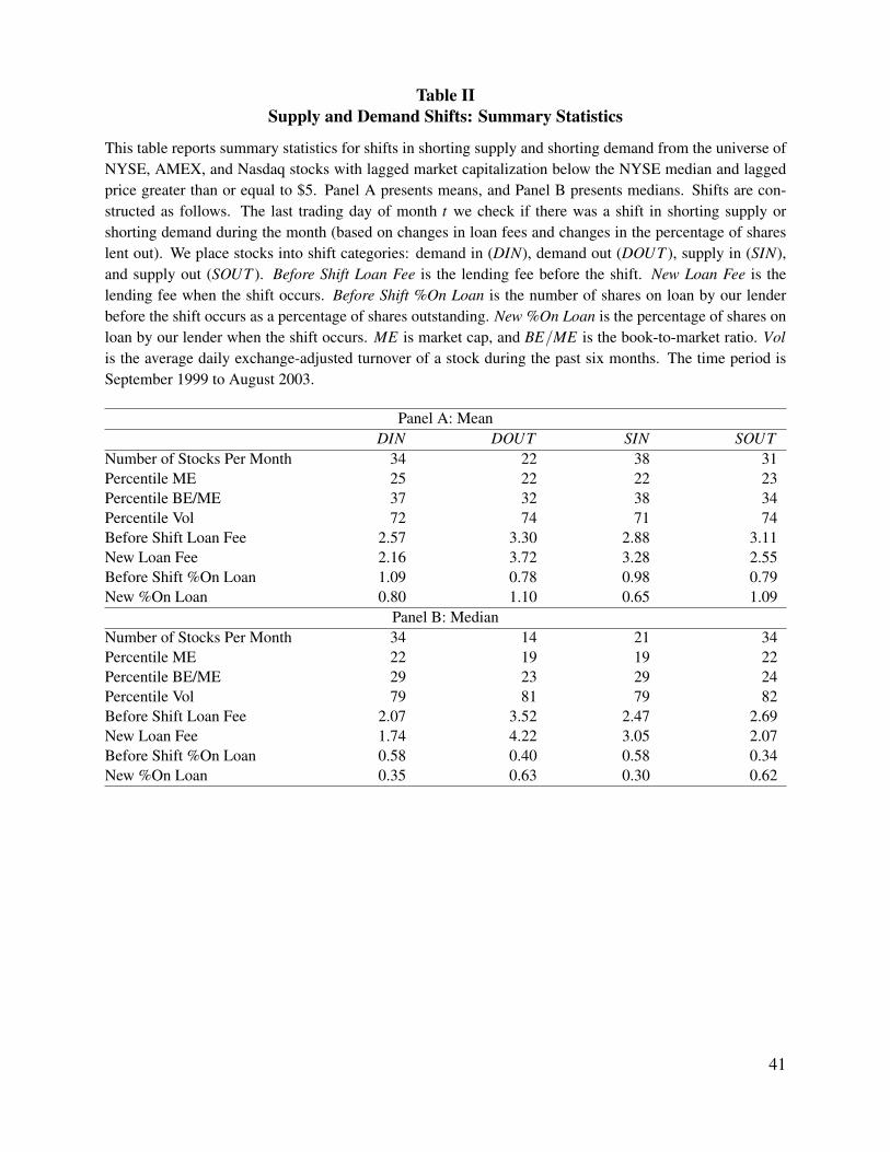
Table IISupply and Demand Shifts: Summary Statistics

This table reports summary statistics for shifts in shorting supply and shorting demand from the universe ofNYSE, AMEX, and Nasdaq stocks with lagged market capitalization below the NYSE median and laggedprice greater than or equal to $5. Panel A presents means, and Panel B presents medians. Shifts are con-structed as follows. The last trading day of month t we check if there was a shift in shorting supply orshorting demand during the month (based on changes in loan fees and changes in the percentage of shareslent out). We place stocks into shift categories: demand in (DIN), demand out (DOUT ), supply in (SIN),and supply out (SOUT ). Before Shift Loan Fee is the lending fee before the shift. New Loan Fee is thelending fee when the shift occurs. Before Shift %On Loan is the number of shares on loan by our lenderbefore the shift occurs as a percentage of shares outstanding. New %On Loan is the percentage of shares onloan by our lender when the shift occurs. ME is market cap, and BE/ME is the book-to-market ratio. Volis the average daily exchange-adjusted turnover of a stock during the past six months. The time period isSeptember 1999 to August 2003.

Panel A: MeanDIN DOUT SIN SOUT

Number of Stocks Per Month 34 22 38 31Percentile ME 25 22 22 23Percentile BE/ME 37 32 38 34Percentile Vol 72 74 71 74Before Shift Loan Fee 2.57 3.30 2.88 3.11New Loan Fee 2.16 3.72 3.28 2.55Before Shift %On Loan 1.09 0.78 0.98 0.79New %On Loan 0.80 1.10 0.65 1.09

Panel B: MedianNumber of Stocks Per Month 34 14 21 34Percentile ME 22 19 19 22Percentile BE/ME 29 23 29 24Percentile Vol 79 81 79 82Before Shift Loan Fee 2.07 3.52 2.47 2.69New Loan Fee 1.74 4.22 3.05 2.07Before Shift %On Loan 0.58 0.40 0.58 0.34New %On Loan 0.35 0.63 0.30 0.62

41

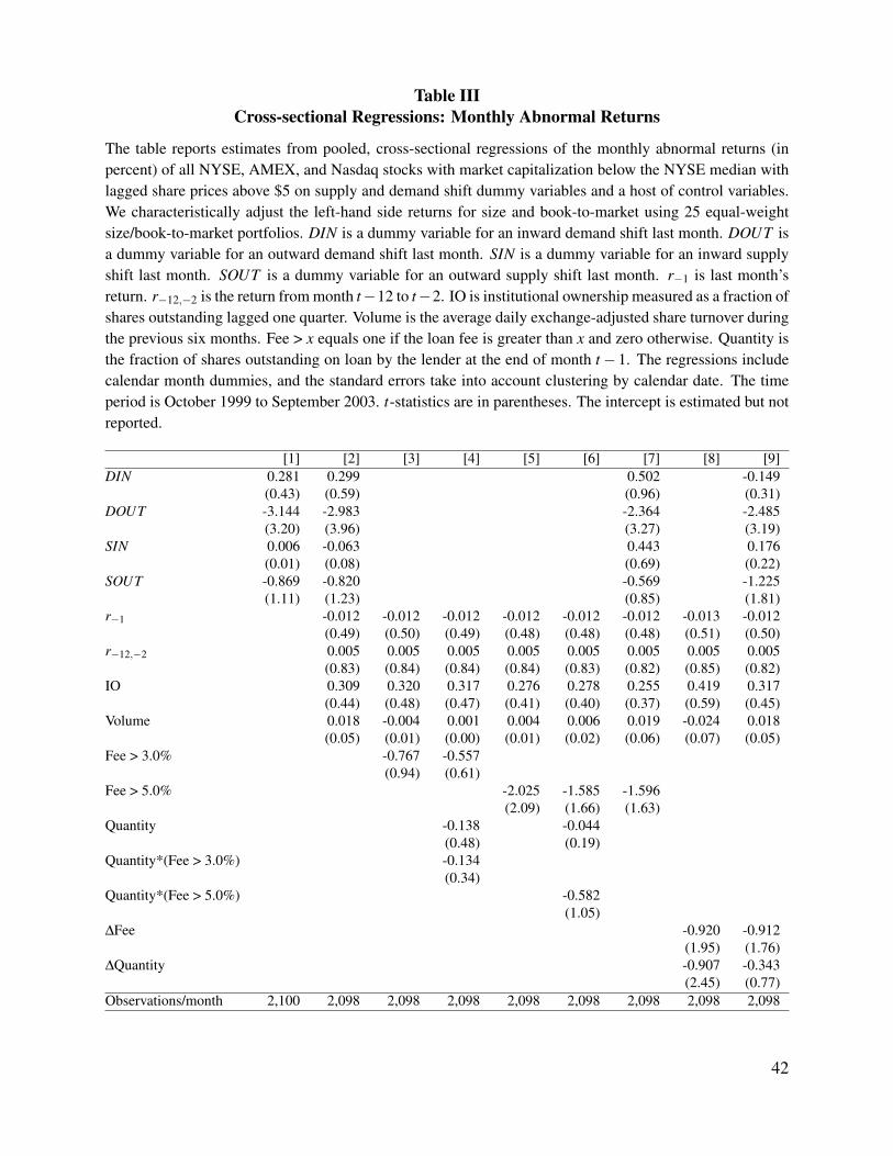
Table IIICross-sectional Regressions: Monthly Abnormal Returns

The table reports estimates from pooled, cross-sectional regressions of the monthly abnormal returns (inpercent) of all NYSE, AMEX, and Nasdaq stocks with market capitalization below the NYSE median withlagged share prices above $5 on supply and demand shift dummy variables and a host of control variables.We characteristically adjust the left-hand side returns for size and book-to-market using 25 equal-weightsize/book-to-market portfolios. DIN is a dummy variable for an inward demand shift last month. DOUT isa dummy variable for an outward demand shift last month. SIN is a dummy variable for an inward supplyshift last month. SOUT is a dummy variable for an outward supply shift last month. r−1 is last month’sreturn. r−12,−2 is the return from month t−12 to t−2. IO is institutional ownership measured as a fraction ofshares outstanding lagged one quarter. Volume is the average daily exchange-adjusted share turnover duringthe previous six months. Fee > x equals one if the loan fee is greater than x and zero otherwise. Quantity isthe fraction of shares outstanding on loan by the lender at the end of month t− 1. The regressions includecalendar month dummies, and the standard errors take into account clustering by calendar date. The timeperiod is October 1999 to September 2003. t-statistics are in parentheses. The intercept is estimated but notreported.

[1] [2] [3] [4] [5] [6] [7] [8] [9]DIN 0.281 0.299 0.502 -0.149

(0.43) (0.59) (0.96) (0.31)DOUT -3.144 -2.983 -2.364 -2.485

(3.20) (3.96) (3.27) (3.19)SIN 0.006 -0.063 0.443 0.176

(0.01) (0.08) (0.69) (0.22)SOUT -0.869 -0.820 -0.569 -1.225

(1.11) (1.23) (0.85) (1.81)r−1 -0.012 -0.012 -0.012 -0.012 -0.012 -0.012 -0.013 -0.012

(0.49) (0.50) (0.49) (0.48) (0.48) (0.48) (0.51) (0.50)r−12,−2 0.005 0.005 0.005 0.005 0.005 0.005 0.005 0.005

(0.83) (0.84) (0.84) (0.84) (0.83) (0.82) (0.85) (0.82)IO 0.309 0.320 0.317 0.276 0.278 0.255 0.419 0.317

(0.44) (0.48) (0.47) (0.41) (0.40) (0.37) (0.59) (0.45)Volume 0.018 -0.004 0.001 0.004 0.006 0.019 -0.024 0.018

(0.05) (0.01) (0.00) (0.01) (0.02) (0.06) (0.07) (0.05)Fee > 3.0% -0.767 -0.557

(0.94) (0.61)Fee > 5.0% -2.025 -1.585 -1.596

(2.09) (1.66) (1.63)Quantity -0.138 -0.044

(0.48) (0.19)Quantity*(Fee > 3.0%) -0.134

(0.34)Quantity*(Fee > 5.0%) -0.582

(1.05)∆Fee -0.920 -0.912

(1.95) (1.76)∆Quantity -0.907 -0.343

(2.45) (0.77)Observations/month 2,100 2,098 2,098 2,098 2,098 2,098 2,098 2,098 2,098

42

Table IVCross-sectional Regressions: Large Shifts and High Loan Fees

The table reports estimates from pooled, cross-sectional regressions of the monthly abnormal returns (in percent) of allNYSE, AMEX, and Nasdaq stocks with market capitalization below the NYSE median with lagged share prices above$5 on supply and demand shifts and control variables. We characteristically adjust the left-hand side returns for sizeand book-to-market using 25 equal-weight size/book-to-market portfolios. We also interact the supply and demandshifts with loan fee and quantity changes. DIN (DOUT ) is a dummy variable for an inward (outward) demand shiftlast month, and SIN (SOUT ) a dummy variable for an inward (outward) supply shift last month. Fee > 3% is a dummyvariable that equals one if the loan fee is greater than 3%. ∆Fee+

big (∆Fee−big) is a dummy variable that equals one if thechange in the loan fee for month t− 1 is greater than (less than or equal to) the 90th (10th) percentile. ∆Quantity+

big

is a dummy variable that equals one if the change in quantity on loan (as a percentage of shares outstanding) formonth t− 1 is greater than the 90th percentile. r−1 is last month’s return. r−12,−2 is the return from month t− 12 tot−2. IO is institutional ownership as a fraction of shares outstanding lagged one quarter. Volume is the average dailyexchange-adjusted share turnover during the previous six months. All regressions include calendar month dummies,and all standard errors take into account clustering by calendar date. The time period is October 1999 to September2003. t-statistics are in parentheses. The intercept is estimated but not reported.

[1] [2] [3] [4] [5] [6]DIN 0.299 0.297 0.298 0.294 0.365 -0.613

(0.59) (0.58) (0.59) (0.58) (0.69) (1.01)DOUT -2.983 -2.649 -2.649 -2.458 -2.866 -0.769

(3.96) (2.66) (2.81) (2.95) (3.40) (0.97)SIN -0.063 -0.062 -0.063 -0.059 0.038 0.655

(0.08) (0.08) (0.08) (0.07) (0.05) (0.88)SOUT -0.820 -0.819 -1.175 -1.136 -0.744 -0.624

(1.23) (0.98) (1.53) (1.53) (1.17) (0.95)DOUT ∗∆Fee+

big -1.253(0.69)

SOUT ∗∆Fee−big -0.015(0.01)

DOUT ∗∆Quantity+big -1.138

(0.67)SOUT ∗∆Quantity+

big 1.169(1.02)

∆Fee+big ∗∆Quantity+

big -4.480(2.32)

∆Fee−big ∗∆Quantity+big 2.633

(1.32)Fee > 3% -0.219 0.175

(0.24) (0.24)(Fee > 3%)*DIN 2.798

(1.82)(Fee > 3%)*DOUT -4.144

(2.69)(Fee > 3%)*SIN -1.691

(0.93)(Fee > 3%)*SOUT -0.710

(0.42)Observations/month 2,098 2,098 2,098 2,098 2,098 2,098Control Variables r−1, r−12,−2, IO, Volume, and calendar month dummies

43

Table VSupply and Demand Shifts: Monthly Portfolio Returns (in percent)

This table presents average monthly returns (in percent) on shorting supply and shorting demand shift port-folios from the universe of NYSE, AMEX, and Nasdaq stocks with lagged market capitalization below theNYSE median and lagged price greater than or equal to $5. Excess Returns are average monthly returns inexcess of the one-month Treasury bill rate. Abnormal Returns are computed by characteristically adjustingreturns using 25 equal weight size/book-to-market portfolios and 75 (3x5x5) equal weight size/book-to-market/momentum portfolios. The benchmark portfolios also contain the restriction that lagged price mustbe greater than or equal to $5. For the last trading day of month t−1 we check if there was a shift in shortingsupply or shorting demand during the month (based on changes in loan fees and changes in the percentageof shares lent out). We place stocks into shift portfolios: demand in (DIN), demand out (DOUT ), supplyin (SIN), and supply out (SOUT ). Shift portfolios are formed in month t−1 and the stocks are held in theportfolios during month t. The time period is October 1999 to September 2003.

Panel A: Excess ReturnsDIN DOUT SIN SOUT DIN−DOUT SIN−SOUT

Equal-WeightMean 1.65 -1.82 0.84 -1.12 3.48 1.96t-stat 0.79 -1.02 0.49 -0.57 2.34 1.55Value-WeightMean 0.53 -0.53 0.42 -2.15 1.06 2.57t-stat 0.27 -0.27 0.23 -1.09 0.65 1.92

Panel B: Abnormal Returns (Benchmark Portfolios: 25 Size/Book-to-Market Portfolios)DIN DOUT SIN SOUT DIN−DOUT SIN−SOUT

Equal-WeightMean 0.84 -2.34 0.48 -1.81 3.18 2.28t-stat 0.67 -2.52 0.56 -1.43 2.17 1.81Value-WeightMean -0.12 -1.05 0.01 -2.63 0.93 2.65t-stat -0.12 -0.88 0.01 -2.23 0.56 1.94

Panel C: Abnormal Returns (Benchmark Portfolios: 75 Size/Book-to-Market/Momentum Portfolios)DIN DOUT SIN SOUT DIN−DOUT SIN−SOUT

Equal-WeightMean 0.76 -2.11 0.08 -1.63 2.87 1.72t-stat 0.72 -2.15 0.11 -1.36 2.21 1.34Value-WeightMean -0.26 -0.88 -0.29 -2.41 0.61 2.12t-stat -0.28 -0.75 -0.30 -2.15 0.41 1.58

44

Table VICross Sectional Regressions: Robustness Tests

The table reports estimates from pooled, cross-sectional regressions of the monthly abnormal returns (in percent)of all NYSE, AMEX, and Nasdaq stocks owned by the lender with market capitalization below the NYSE medianand lagged share prices above $5 on supply and demand shift dummy variables and a host of control variables. Wecharacteristically adjust all left-hand side returns for size and book-to-market using 25 equal-weight size-BE/MEportfolios. DIN (DOUT ) is a dummy variable for an inward (outward) demand shift last month , and SIN (SOUT ) adummy variable for an inward (outward) supply shift last month. In columns 1 to 4, the loan quantity used to defineshifts is the number of shares on loan by our lender divided by total shares outstanding (%On Loan), and returns aremeasured at the month’s end; in column 5, loan quantity equals total monthly short interest divided by total sharesoutstanding (Short Int), and monthly returns are measured using closing prices from the 16th of the month. MarketPower is the number of shares lent out by our lender in month t−1 divided by short interest (SI) in month t−1, whileMarket Power > 2/3 is a dummy variable equal to one if the lender’s Market Power exceeds two-thirds. r−1 is lastmonth’s return. r−12,−2 is the return from month t− 12 to t− 2. IO is institutional ownership as a fraction of sharesoutstanding lagged one quarter. Volume is the average daily exchange-adjusted share turnover during the previoussix months. All five columns include calendar month dummies, and the first column also includes industry dummies(using Fama and French’s (1997) 48-industry classification scheme). All standard errors take into account clusteringby calendar date. The time period is October 1999 to September 2003 for columns 1 to 4 and November 1999 toSeptember 2003 for column 5. t-statistics are in parentheses. The intercept is estimated but not reported.

[1] [2] [3] [4] [5]DIN 0.206 0.273 0.196 0.356 0.215

(0.41) (0.53) (0.34) (0.69) (0.42)DOUT -3.030 -3.014 -2.389 -2.741 -1.262

(4.05) (3.94) (3.03) (3.52) (2.06)SIN -0.172 -0.067 0.156 0.009 -0.950

(0.22) (0.08) (0.18) (0.01) (1.22)SOUT -0.888 -0.804 -0.731 -0.803 -0.793

(1.35) (1.21) (1.17) (1.25) (1.48)(Market Power)*DIN 0.585

(0.25)(Market Power)*DOUT -5.642

(1.26)(Market Power)*SIN -1.537

(0.56)(Market Power)*SOUT -0.683

(0.24)(Market Power>2/3)*DIN -1.446

(0.77)(Market Power>2/3)*DOUT -8.361

(2.38)(Market Power>2/3)*SIN -1.296

(0.57)(Market Power>2/3)*SOUT 0.050

(0.01)Observations/month 2,098 2,095 2,095 2,095 2,097Loan Quantity %On Loan %On Loan %On Loan %On Loan Short IntIndustry Dummies Yes No No No NoControl Variables r−1,r−12,−2, IO, Volume, and calendar month dummies always included

45

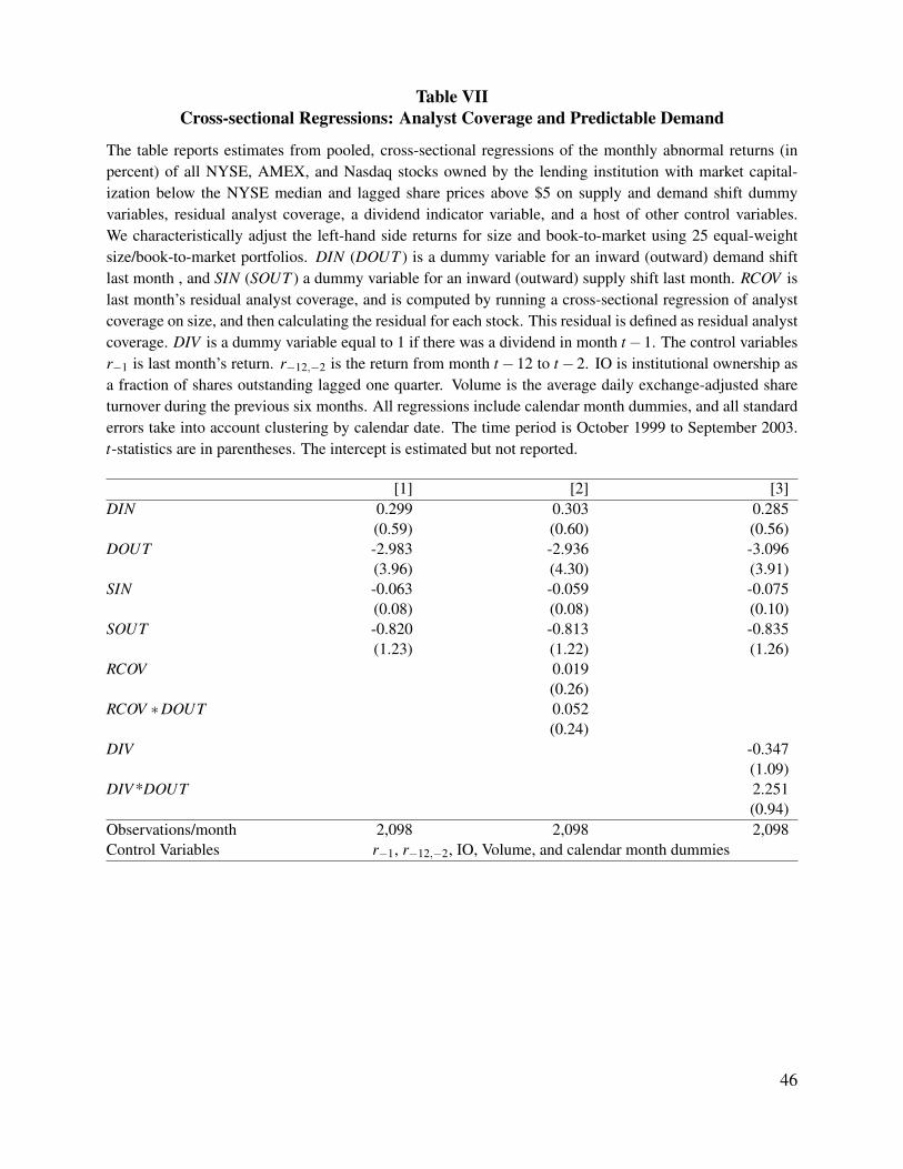
Table VIICross-sectional Regressions: Analyst Coverage and Predictable Demand

The table reports estimates from pooled, cross-sectional regressions of the monthly abnormal returns (inpercent) of all NYSE, AMEX, and Nasdaq stocks owned by the lending institution with market capital-ization below the NYSE median and lagged share prices above $5 on supply and demand shift dummyvariables, residual analyst coverage, a dividend indicator variable, and a host of other control variables.We characteristically adjust the left-hand side returns for size and book-to-market using 25 equal-weightsize/book-to-market portfolios. DIN (DOUT ) is a dummy variable for an inward (outward) demand shiftlast month , and SIN (SOUT ) a dummy variable for an inward (outward) supply shift last month. RCOV islast month’s residual analyst coverage, and is computed by running a cross-sectional regression of analystcoverage on size, and then calculating the residual for each stock. This residual is defined as residual analystcoverage. DIV is a dummy variable equal to 1 if there was a dividend in month t−1. The control variablesr−1 is last month’s return. r−12,−2 is the return from month t−12 to t−2. IO is institutional ownership asa fraction of shares outstanding lagged one quarter. Volume is the average daily exchange-adjusted shareturnover during the previous six months. All regressions include calendar month dummies, and all standarderrors take into account clustering by calendar date. The time period is October 1999 to September 2003.t-statistics are in parentheses. The intercept is estimated but not reported.

[1] [2] [3]DIN 0.299 0.303 0.285

(0.59) (0.60) (0.56)DOUT -2.983 -2.936 -3.096

(3.96) (4.30) (3.91)SIN -0.063 -0.059 -0.075

(0.08) (0.08) (0.10)SOUT -0.820 -0.813 -0.835

(1.23) (1.22) (1.26)RCOV 0.019

(0.26)RCOV ∗DOUT 0.052

(0.24)DIV -0.347

(1.09)DIV *DOUT 2.251

(0.94)Observations/month 2,098 2,098 2,098Control Variables r−1, r−12,−2, IO, Volume, and calendar month dummies

46

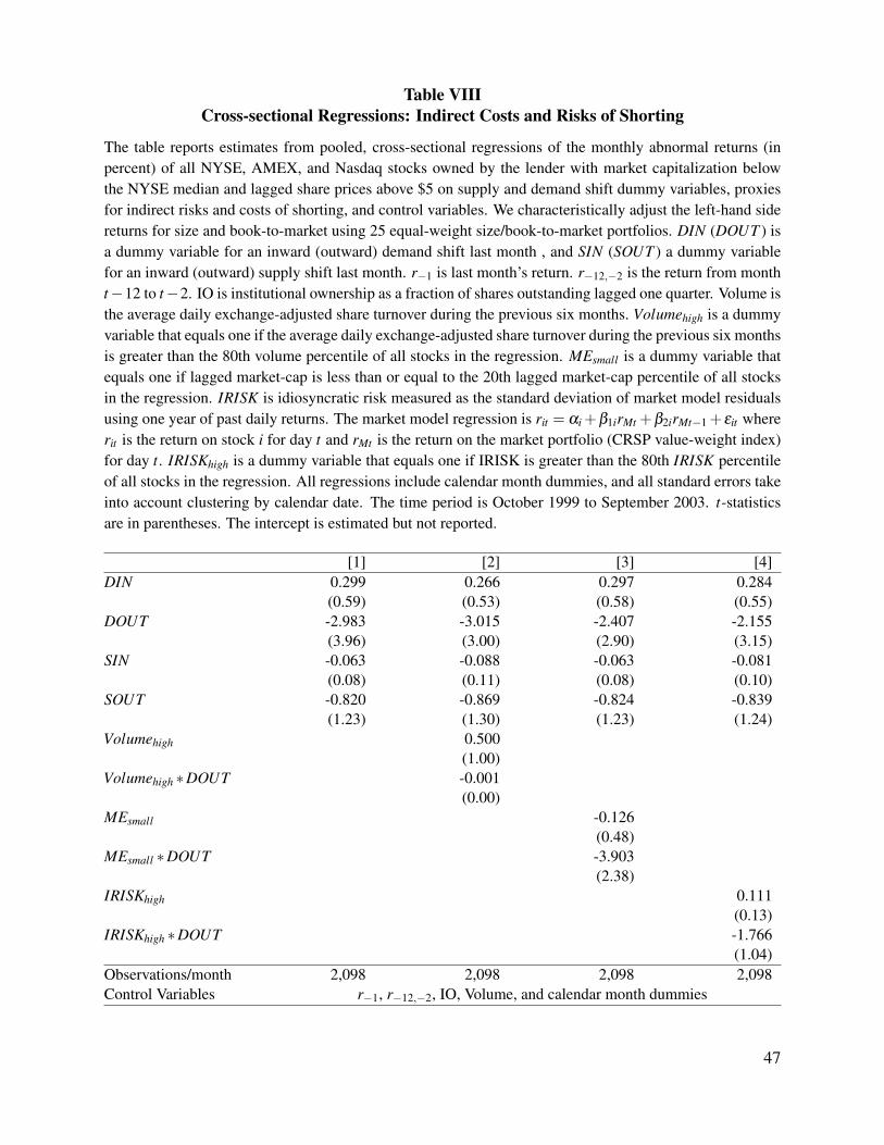
Table VIIICross-sectional Regressions: Indirect Costs and Risks of Shorting

The table reports estimates from pooled, cross-sectional regressions of the monthly abnormal returns (inpercent) of all NYSE, AMEX, and Nasdaq stocks owned by the lender with market capitalization belowthe NYSE median and lagged share prices above $5 on supply and demand shift dummy variables, proxiesfor indirect risks and costs of shorting, and control variables. We characteristically adjust the left-hand sidereturns for size and book-to-market using 25 equal-weight size/book-to-market portfolios. DIN (DOUT ) isa dummy variable for an inward (outward) demand shift last month , and SIN (SOUT ) a dummy variablefor an inward (outward) supply shift last month. r−1 is last month’s return. r−12,−2 is the return from montht−12 to t−2. IO is institutional ownership as a fraction of shares outstanding lagged one quarter. Volume isthe average daily exchange-adjusted share turnover during the previous six months. Volumehigh is a dummyvariable that equals one if the average daily exchange-adjusted share turnover during the previous six monthsis greater than the 80th volume percentile of all stocks in the regression. MEsmall is a dummy variable thatequals one if lagged market-cap is less than or equal to the 20th lagged market-cap percentile of all stocksin the regression. IRISK is idiosyncratic risk measured as the standard deviation of market model residualsusing one year of past daily returns. The market model regression is rit = αi +β1irMt +β2irMt−1 +εit whererit is the return on stock i for day t and rMt is the return on the market portfolio (CRSP value-weight index)for day t. IRISKhigh is a dummy variable that equals one if IRISK is greater than the 80th IRISK percentileof all stocks in the regression. All regressions include calendar month dummies, and all standard errors takeinto account clustering by calendar date. The time period is October 1999 to September 2003. t-statisticsare in parentheses. The intercept is estimated but not reported.

[1] [2] [3] [4]DIN 0.299 0.266 0.297 0.284

(0.59) (0.53) (0.58) (0.55)DOUT -2.983 -3.015 -2.407 -2.155

(3.96) (3.00) (2.90) (3.15)SIN -0.063 -0.088 -0.063 -0.081

(0.08) (0.11) (0.08) (0.10)SOUT -0.820 -0.869 -0.824 -0.839

(1.23) (1.30) (1.23) (1.24)Volumehigh 0.500

(1.00)Volumehigh ∗DOUT -0.001

(0.00)MEsmall -0.126

(0.48)MEsmall ∗DOUT -3.903

(2.38)IRISKhigh 0.111

(0.13)IRISKhigh ∗DOUT -1.766

(1.04)Observations/month 2,098 2,098 2,098 2,098Control Variables r−1, r−12,−2, IO, Volume, and calendar month dummies

47

-0.3%-0.25%-0.2%

-0.15%-0.1%

-0.05%0%

0.05%0.1%

0.15%0.2%

0.25%0.3%

t-5t-4t-3t-2t-1t

Co

eff

icie

nt:

DO

UT

(t-l

ag

)

Lag in Days

Daily Abnormal Returns & Lagged DOUT

DOUT(t-lag) regression coefficient95% Confidence Interval

-1.5%-1.2%-0.9%-0.6%-0.3%

0%0.3%0.6%0.9%1.2%1.5%

t-4t-3t-2t-1

Co

eff

icie

nt:

DO

UT

(t-l

ag

)

Lag in Weeks

Weekly Abnormal Returns & Lagged DOUT

DOUT(t-lag) regression coefficient95% Confidence Interval

-6%-5%-4%-3%-2%-1%0%1%2%3%4%5%6%

t-6t-5t-4t-3t-2t-1

Co

eff

icie

nt:

DO

UT

(t-l

ag

)

Lag in Months

Monthly Abnormal Returns & Lagged DOUT

DOUT(t-lag) regression coefficient95% Confidence Interval

-0.3%-0.25%-0.2%

-0.15%-0.1%

-0.05%0%

0.05%0.1%

0.15%0.2%

0.25%0.3%

t-5t-4t-3t-2t-1t

Co

eff

icie

nt:

SO

UT

(t-l

ag

)

Lag in Days

Daily Abnormal Returns & Lagged SOUT

DOUT(t-lag) regression coefficient95% Confidence Interval

-1.5%-1.2%-0.9%-0.6%-0.3%

0%0.3%0.6%0.9%1.2%1.5%

t-4t-3t-2t-1

Co

eff

icie

nt:

SO

UT

(t-l

ag

)

Lag in Weeks

Weekly Abnormal Returns & Lagged SOUT

DOUT(t-lag) regression coefficient95% Confidence Interval

-6%-5%-4%-3%-2%-1%0%1%2%3%4%5%6%

t-6t-5t-4t-3t-2t-1

Co

eff

icie

nt:

SO

UT

(t-l

ag

)

Lag in Months

Monthly Abnormal Returns & Lagged SOUT

DOUT(t-lag) regression coefficient95% Confidence Interval

Figure 1. Daily , weekly, and monthly abnormal returns. In the top row we regress the daily abnormal returns

(in percent) of all stocks owned by the lender with market capitalization below the NYSE median and lagged share

prices above $5 on daily supply and demand shifts and lagged daily returns. In row 2 (row 3) we regress the weekly

(monthly) abnormal returns (in percent) of the same universe of stocks on weekly (monthly) supply and demand

shifts. We include all the shifts in the regressions (DIN, DOUT, SIN, and SOUT), but only report the coefficients for

DOUT and SOUT. DOUT(t-lag) is a dummy variable for an outward demand shift lag days (weeks, months) ago, and

SOUT(t-lag) is a dummy variable for an outward supply shift lag days (weeks, months) ago. We proxy for expected

returns characteristically using 25 equal-weight size/book-to-market portfolios. We run separate regressions for each

lag length. The regressions include calendar time dummies, and the standard errors take into account clustering by

calendar date.

48