advances.sciencemag.org/cgi/content/full/2/1/e1501014/DC1

Supplementary Materials for

An iron-iron hydrogenase mimic with appended electron reservoir for

efficient proton reduction in aqueous media

René Becker, Saeed Amirjalayer, Ping Li, Sander Woutersen, Joost N. H. Reek

Published 22 January 2016, Sci. Adv. 2, e1501014 (2016)

DOI: 10.1126/sciadv.1501014

The PDF file includes:

Materials and Methods

Fig. S1. Solution IR spectra of 1, 1Ph, and Et21·(BF4)2 in dichloromethane.

Fig. S2. 1H NMR (400 MHz) of 1 in CD2Cl2.

Fig. S3. 31P NMR (162 MHz) of 1 in CD2Cl2.

Fig. S4. 1H1H correlation spectroscopy (COSY; 300 MHz) of 1 in CD2Cl2.

Fig. S5. Nuclear Overhauser effect spectroscopy (NOESY; 300 MHz) of 1 in

CD2Cl2.

Fig. S6. 1H NMR (400 MHz) of 1Ph in CD2Cl2.

Fig. S7. 31P NMR (162 MHz) of 1Ph in CD2Cl2.

Fig. S8. FD mass analysis of 1.

Fig. S9. FD mass analysis of 1Ph.

Fig. S10. X-ray diffraction structure of 1Ph with displacement ellipsoids at 50%

probability.

Fig. S11. Bulk electrolysis of 10 μmol 1 on a carbon sponge electrode.

Fig. S12. Integrated data from fig. S11.

Fig. S13. Cyclic voltammograms of 0.5 mM 1.

Fig. S14. Cyclic voltammograms of 0.5 mM 1, starting from −1.6 V to the

cathodic peak, then cycling over the reoxidation wave.

Fig. S15. Simulation of cyclic voltammograms (DigiElch) from fig. S13 (scan

rate, 0.1 V s−1).

Fig. S16. Simulation of cyclic voltammograms (DigiElch) from fig. S13 (scan

rate, 1.0 V s−1).

Fig. S17. UV-vis spectra of 1 and ZnTPP at a path length of 10 mm.

Fig. S18. UV-vis titration of a constant concentration of 80 μM ZnTPP with

increasing equivalents 1.

Fig. S19. Output of the fitting procedure.

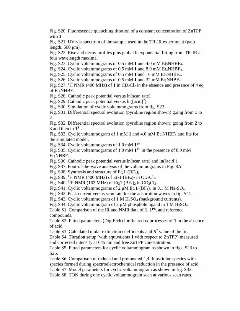
Fig. S20. Fluorescence quenching titration of a constant concentration of ZnTPP

with 1.

Fig. S21. UV-vis spectrum of the sample used in the TR-IR experiment (path

length, 500 μm).

Fig. S22. Rise and decay profiles plus global biexponential fitting from TR-IR at

four wavelength maxima.

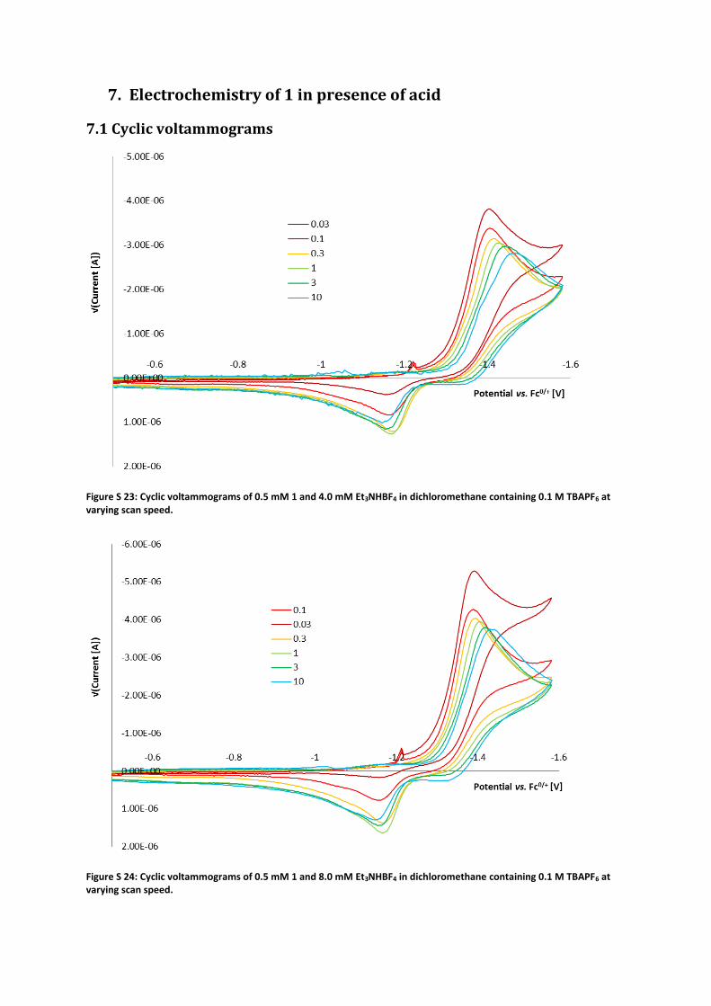
Fig. S23. Cyclic voltammograms of 0.5 mM 1 and 4.0 mM Et3NHBF4.

Fig. S24. Cyclic voltammograms of 0.5 mM 1 and 8.0 mM Et3NHBF4.

Fig. S25. Cyclic voltammograms of 0.5 mM 1 and 16 mM Et3NHBF4.

Fig. S26. Cyclic voltammograms of 0.5 mM 1 and 32 mM Et3NHBF4.

Fig. S27. 1H NMR (400 MHz) of 1 in CD2Cl2 in the absence and presence of 4 eq

of Et3NHBF4.

Fig. S28. Cathodic peak potential versus ln(scan rate).

Fig. S29. Cathodic peak potential versus ln([acid]2).

Fig. S30. Simulation of cyclic voltammograms from fig. S23.

Fig. S31. Differential spectral evolution (pyridine region shown) going from 1 to

2.

Fig. S32. Differential spectral evolution (pyridine region shown) going from 2 to

3 and then to 13−.

Fig. S33. Cyclic voltammogram of 1 mM 1 and 4.0 mM Et3NHBF4 and fits for

the simulated model.

Fig. S34. Cyclic voltammograms of 1.0 mM 1Ph.

Fig. S35. Cyclic voltammograms of 1.0 mM 1Ph in the presence of 8.0 mM

Et3NHBF4.

Fig. S36. Cathodic peak potential versus ln(scan rate) and ln([acid]).

Fig. S37. Foot-of-the-wave analysis of the voltammograms in Fig. 8A.

Fig. S38. Synthesis and structure of Et21·(BF4)2.

Fig. S39. 1H NMR (400 MHz) of Et21·(BF4)2 in CD2Cl2.

Fig. S40. 31P NMR (162 MHz) of Et21·(BF4)2 in CD2Cl2.

Fig. S41. Cyclic voltammograms of 2 μM Et21·(BF4)2 in 0.1 M Na2SO4.

Fig. S42. Peak current versus scan rate for the adsorption waves in fig. S41.

Fig. S43. Cyclic voltammogram of 1 M H2SO4 (background currents).

Fig. S44. Cyclic voltammogram of 2 μM phosphole ligand in 1 M H2SO4.

Table S1. Comparison of the IR and NMR data of 1, 1Ph, and reference

compounds.

Table S2. Fitted parameters (DigiElch) for the redox processes of 1 in the absence

of acid.

Table S3. Calculated molar extinction coefficients and R2 value of the fit.

Table S4. Titration setup (with equivalents 1 with respect to ZnTPP) measured

and corrected intensity at 645 nm and free ZnTPP concentration.

Table S5. Fitted parameters for cyclic voltammogram as shown in figs. S23 to

S26.

Table S6. Comparison of reduced and protonated 4,4′-bipyridine species with

species formed during spectroelectrochemical reduction in the presence of acid.

Table S7. Model parameters for cyclic voltammogram as shown in fig. S33.

Table S8. TON during one cyclic voltammogram scan at various scan rates.

References (46–48)

1. Materials and methods

1.1 NMR and EPR spectroscopy The 1H and 31P NMR spectra were measured on a Bruker AV400 spectrometer. The 1H1H-COSY and

NOESY spectra were measured on a Bruker AV300 spectrometer. Experimental X-band EPR spectra

were recorded on a Bruker EMX spectrometer (Bruker BioSpin Rheinstetten) equipped with a He

temperature control cryostat system (Oxford Instruments), on an ELEXSYS 680 spectrometer and

using an in-house developed setup based on the resonator ER4116X-MD-5-W1. Chemical reduction

was performed (in a glove box) on ~0.1 mM 1 and CoCp*2 (2 equiv.) in toluene at room temperature.

1.2 Steady state UV-vis, fluorescence and infrared spectroscopy IR measurements were conducted on a Thermo Nicolet Nexus FT-IR spectrometer. UV-vis

measurements were conducted on a Hewlett-Packard 8453 spectrometer. Fluorescence

measurements were conducted on a Spex Fluorolog 3 spectrometer.

1.3 Spectroelectrochemistry IR spectroelectrochemical measurements were performed with an optically transparent thin-layer

electrochemical (OTTLE) cell equipped with CaF2 optical windows and either a micro-grid platinum or

a mini-grid gold-amalgam working electrode (45). The optical beam can pass directly through the

working electrode, allowing the redox processes taking place in the thin solution layer surrounding

the working electrode to be monitored spectroscopically. The controlled-potential electrochemical

conversions were carried out with a PGSTAT10 potentiostat (Metrohm/Autolab). A slow scan rate of

2 mV/s was applied to allow for semi-quantitative electrochemical conversion. The solutions were

prepared in a similar fashion described for the electrochemistry experiments. IR spectra were

recorded on a Nicolet Nexus FT-IR spectrometer.

1.4 Mass analysis Mass spectra were collected on an AccuTOF GC v 4g, JMS-T100GCV Mass spectrometer (JEOL,

Japan). FD probe equipped with FD Emitter, Carbotec (Germany), FD 10 μm. Current rate 51.2

mA/min over 1.2 min. Typical measurement conditions are: Counter electrode –10kV, Ion source

37V.

1.5 Bulk electrolysis (controlled potential coulometry) Bulk electrolysis was performed on 10 mL of a 1.0 mM solution of 1 in dichloromethane containing

0.1 M nBu4NPF6. The working electrode was made from Duocel reticulated vitreous carbon foam, ca.

1x3x0.3 cm geometric volume (45 PPI, 3% density; ERG Aerospace Corporation, Oakland California).

The reference electrode was identical to the one used in cyclic voltammetry. The counter electrode

was a platinum coil in a separate compartment (containing 5 mL of 0.1 M nBu4NPF6 in

dichloromethane), separated with a vycor frit (P5; porosity 1.0-1.6 µm) from the working solution.

1.6 X-ray Crystal Structure Determination of complex 1Ph X-ray intensities were measured on a Bruker D8 Quest Eco diffractometer equipped with a Triumph

monochromator ( = 0.71073 Å) and a CMOS Photon 50 detector at a temperature of 150(2) K.

Intensity data were integrated with the Bruker APEX2 software (Bruker, APEX2 software, Madison

WI, USA, 2014). Absorption correction and scaling was performed with SADABS (G. M. Sheldrick,

SADABS, Universität Göttingen, Germany, 2008). The structures were solved with the program

SHELXL. Least-squares refinement was performed with SHELXL-2013 (G. M. Sheldrick, SHELXL2013,

Universität Göttingen, Germany, 2013) against F2 of all reflections. Non-hydrogen atoms were

refined with anisotropic displacement parameters. The H atoms were placed at calculated positions

using the instructions AFIX 13, AFIX 43 or AFIX 137 with isotropic displacement parameters having

values 1.2 or 1.5 times Ueq of the attached C atoms. CCDC 1435208 contain the supplementary

crystallographic data for this paper. These data can be obtained free of charge from The Cambridge

Crystallographic Data Centre via http://www.ccdc.cam.ac.uk/data_request/cif/

2. Characterization

2.1 Infrared spectroscopy

Figure S 1: Solution infrared spectrum of 1, 1Ph and Et21.(BF4)2 in dichloromethane. All spectra normalized to the first peak.

2.2 NMR spectroscopy of 1

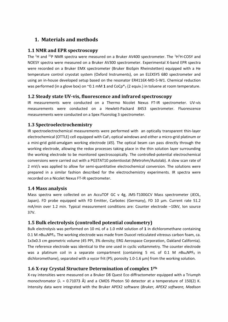
Figure S 2: 1H-NMR (400 MHz) of 1 in CD2Cl2.

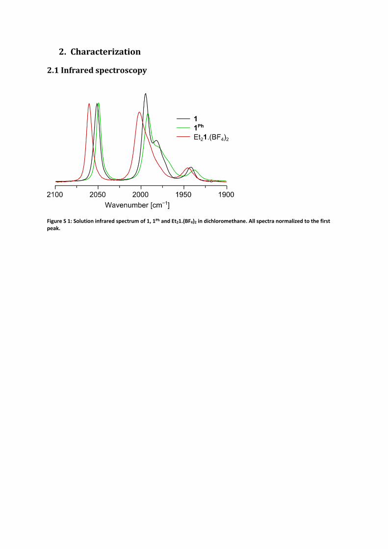
Figure S 3: 31P-NMR (162 MHz) of 1 in CD2Cl2.

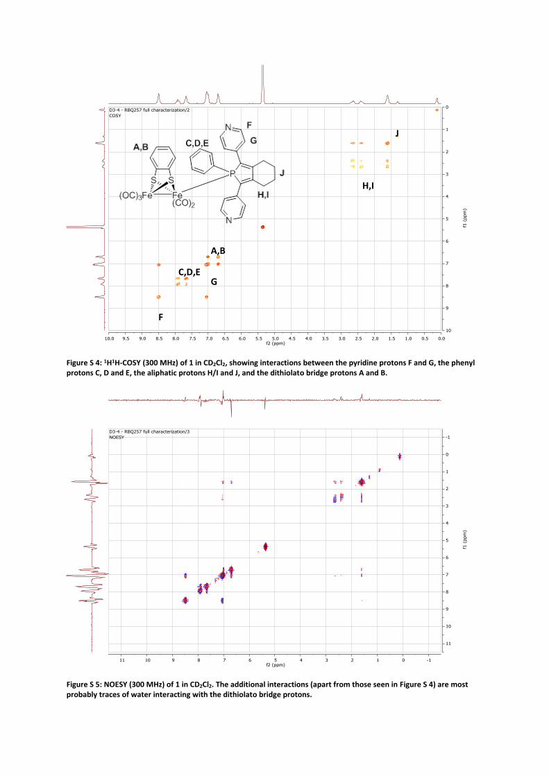
Figure S 4: 1H1H-COSY (300 MHz) of 1 in CD2Cl2, showing interactions between the pyridine protons F and G, the phenyl protons C, D and E, the aliphatic protons H/I and J, and the dithiolato bridge protons A and B.

Figure S 5: NOESY (300 MHz) of 1 in CD2Cl2. The additional interactions (apart from those seen in Figure S 4) are most probably traces of water interacting with the dithiolato bridge protons.

A,B

F

G C,D,E

H,I

J

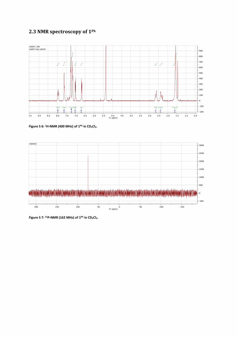
2.3 NMR spectroscopy of 1Ph

Figure S 6: 1H-NMR (400 MHz) of 1Ph in CD2Cl2.

Figure S 7: 31P-NMR (162 MHz) of 1Ph in CD2Cl2.

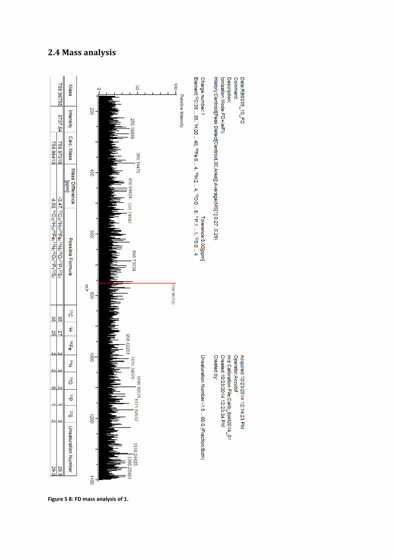
2.4 Mass analysis

Figure S 8: FD mass analysis of 1.

Figure S 9: FD mass analysis of 1Ph.

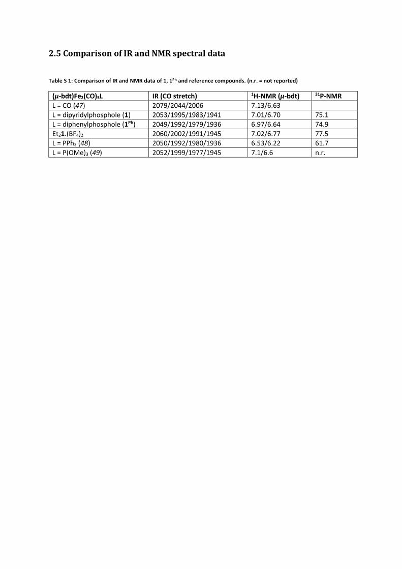
2.5 Comparison of IR and NMR spectral data

Table S 1: Comparison of IR and NMR data of 1, 1Ph and reference compounds. (n.r. = not reported)

(μ-bdt)Fe2(CO)5L IR (CO stretch) 1H-NMR (μ-bdt) 31P-NMR

L = CO (47) 2079/2044/2006 7.13/6.63

L = dipyridylphosphole (1) 2053/1995/1983/1941 7.01/6.70 75.1

L = diphenylphosphole (1Ph) 2049/1992/1979/1936 6.97/6.64 74.9

Et21.(BF4)2 2060/2002/1991/1945 7.02/6.77 77.5

L = PPh3 (48) 2050/1992/1980/1936 6.53/6.22 61.7

L = P(OMe)3 (49) 2052/1999/1977/1945 7.1/6.6 n.r.

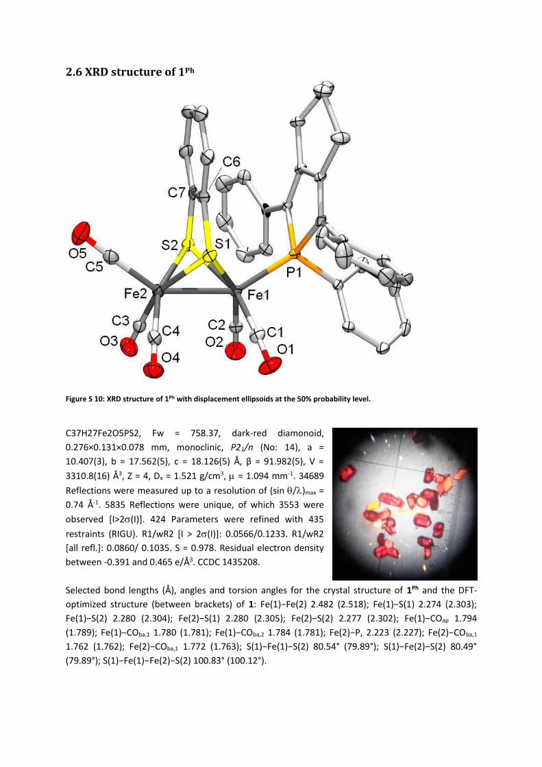
2.6 XRD structure of 1Ph

Figure S 10: XRD structure of 1Ph with displacement ellipsoids at the 50% probability level.

C37H27Fe2O5PS2, Fw = 758.37, dark-red diamonoid,

0.276×0.131×0.078 mm, monoclinic, P21/n (No: 14), a =

10.407(3), b = 17.562(5), c = 18.126(5) Å, β = 91.982(5), V =

3310.8(16) Å3, Z = 4, Dx = 1.521 g/cm3, = 1.094 mm-1. 34689

Reflections were measured up to a resolution of (sin /)max =

0.74 Å-1. 5835 Reflections were unique, of which 3553 were

observed [I>2(I)]. 424 Parameters were refined with 435

restraints (RIGU). R1/wR2 [I > 2(I)]: 0.0566/0.1233. R1/wR2

[all refl.]: 0.0860/ 0.1035. S = 0.978. Residual electron density

between -0.391 and 0.465 e/Å3. CCDC 1435208.

Selected bond lengths (Å), angles and torsion angles for the crystal structure of 1Ph and the DFT-

optimized structure (between brackets) of 1: Fe(1)−Fe(2) 2.482 (2.518); Fe(1)−S(1) 2.274 (2.303);

Fe(1)−S(2) 2.280 (2.304); Fe(2)−S(1) 2.280 (2.305); Fe(2)−S(2) 2.277 (2.302); Fe(1)−COap 1.794

(1.789); Fe(1)−COba,1 1.780 (1.781); Fe(1)−COba,2 1.784 (1.781); Fe(2)−P, 2.223 (2.227); Fe(2)−COba,1

1.762 (1.762); Fe(2)−COba,1 1.772 (1.763); S(1)−Fe(1)−S(2) 80.54° (79.89°); S(1)−Fe(2)−S(2) 80.49°

(79.89°); S(1)−Fe(1)−Fe(2)−S(2) 100.83° (100.12°).

3. Electrochemistry of 1 in absence of acid

Figure S 11: Bulk electrolysis of 10 μmol 1 on a carbon sponge electrode.

Figure S 12: Integrated data from Figure S 11, showing the amount of electrons passed per molecule 1 during electrolysis.

Figure S 13: Cyclic voltammograms of 0.5 mM 1 in dichloromethane containing 0.1 M TBAPF6 at varying scan speed.

Figure S 14: Cyclic voltammograms of 0.5 mM 1 in dichloromethane containing 0.1 M TBAPF6 at varying scan speed, starting from -1.6 V to the cathodic peak, then cycling over the reoxidation wave.

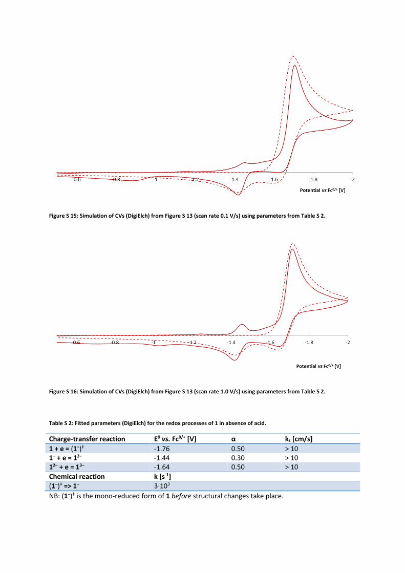
Figure S 15: Simulation of CVs (DigiElch) from Figure S 13 (scan rate 0.1 V/s) using parameters from Table S 2.

Figure S 16: Simulation of CVs (DigiElch) from Figure S 13 (scan rate 1.0 V/s) using parameters from Table S 2.

Table S 2: Fitted parameters (DigiElch) for the redox processes of 1 in absence of acid.

Charge-transfer reaction E0 vs. Fc0/+ [V] α ks [cm/s]

1 + e = (1–)‡ -1.76 0.50 > 10 1– + e = 12– -1.44 0.30 > 10 12– + e = 13– -1.64 0.50 > 10

Chemical reaction k [s-1]

(1–)‡ => 1– 3∙103

NB: (1–)‡ is the mono-reduced form of 1 before structural changes take place.

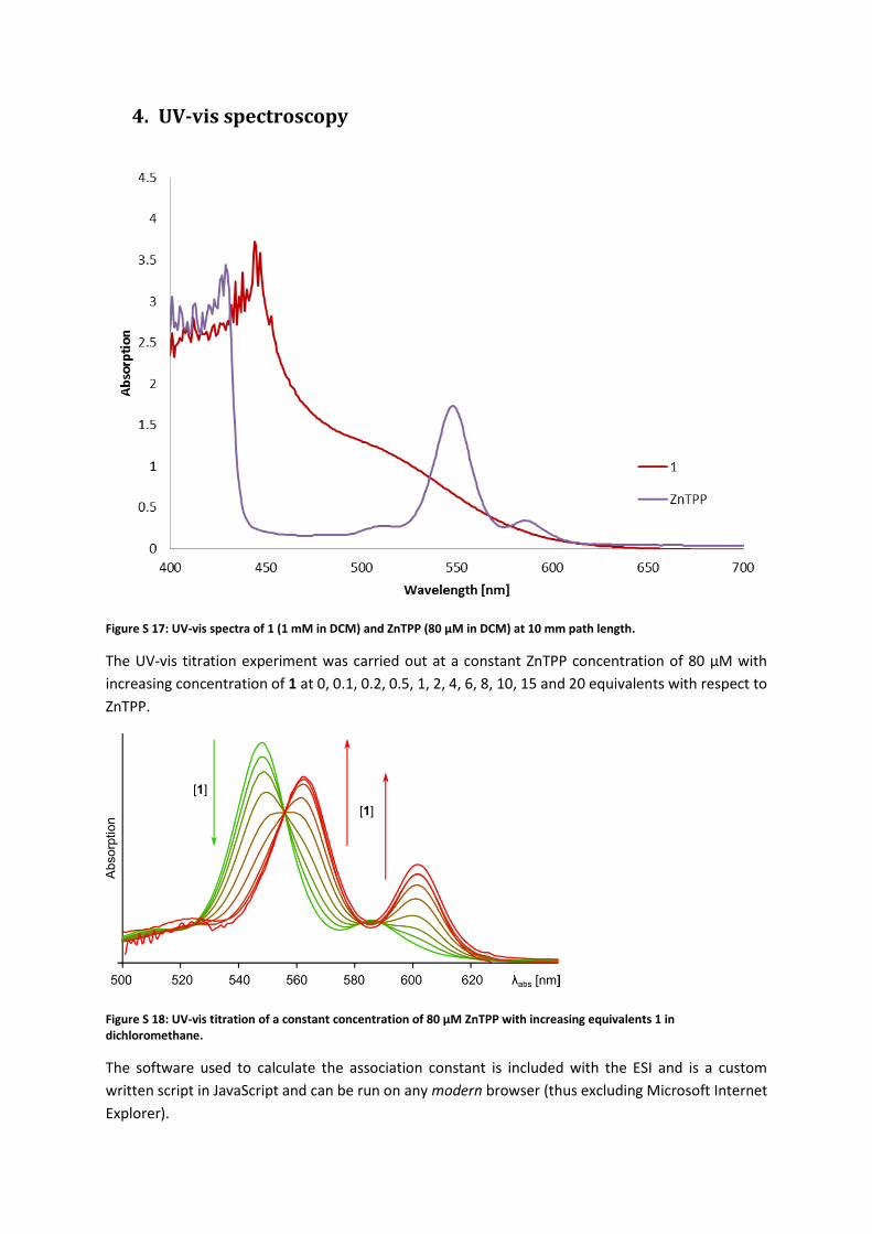
4. UV-vis spectroscopy

Figure S 17: UV-vis spectra of 1 (1 mM in DCM) and ZnTPP (80 µM in DCM) at 10 mm path length.

The UV-vis titration experiment was carried out at a constant ZnTPP concentration of 80 µM with

increasing concentration of 1 at 0, 0.1, 0.2, 0.5, 1, 2, 4, 6, 8, 10, 15 and 20 equivalents with respect to

ZnTPP.

Figure S 18: UV-vis titration of a constant concentration of 80 µM ZnTPP with increasing equivalents 1 in dichloromethane.

The software used to calculate the association constant is included with the ESI and is a custom

written script in JavaScript and can be run on any modern browser (thus excluding Microsoft Internet

Explorer).

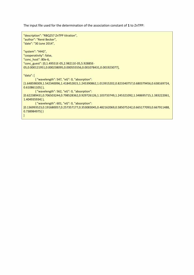
The input file used for the determination of the association constant of 1 to ZnTPP:

"description": "RBQ257 ZnTPP titration", "author": "René Becker", "date": "30 June 2014", "system": "HHG", "cooperativity": false, "conc_host": 80e-6, "conc_guest": [0,1.49551E-05,2.98211E-05,5.92885E-05,0.000121951,0.000238095,0.000555556,0.001078431,0.001923077], "data": [ { "wavelength": 547, "eG": 0, "absorption": [1.648598309,1.542340096,1.418452815,1.245390862,1.013915202,0.823340757,0.680379456,0.638169724,0.610861105] }, { "wavelength": 562, "eG": 0, "absorption": [0.622389431,0.706503244,0.798528362,0.929726126,1.103733749,1.245321092,1.348695715,1.383222061,1.404935934] }, { "wavelength": 601, "eG": 0, "absorption": [0.136993523,0.191680057,0.257357177,0.353083045,0.482162069,0.585075242,0.665177093,0.667911488,0.738984975] } ]

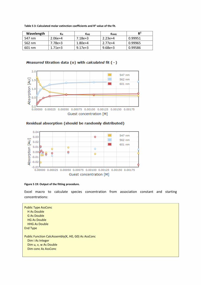
Table S 3: Calculated molar extinction coefficients and R2 value of the fit.

Wavelength εH εHG εHHG R2 547 nm 2.06e+4 7.18e+3 2.23e+4 0.99951 562 nm 7.78e+3 1.80e+4 2.77e+4 0.99965 601 nm 1.71e+3 9.17e+3 9.68e+3 0.99586

Figure S 19: Output of the fitting procedure.

Excel macro to calculate species concentration from association constant and starting

concentrations:

Public Type AssConc H As Double G As Double HG As Double HHG As Double End Type Public Function CalcAssembly(K, H0, G0) As AssConc Dim i As Integer Dim u, v, w As Double Dim conc As AssConc

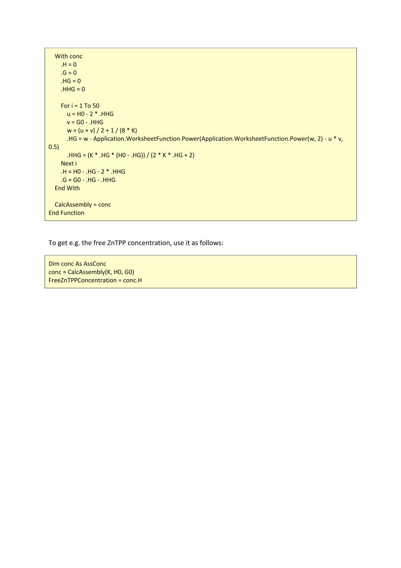
With conc .H = 0 .G = 0 .HG = 0 .HHG = 0 For i = 1 To 50 u = H0 - 2 * .HHG v = G0 - .HHG w = (u + v) / 2 + 1 / (8 * K) .HG = w - Application.WorksheetFunction.Power(Application.WorksheetFunction.Power(w, 2) - u * v, 0.5) .HHG = (K * .HG * (H0 - .HG)) / (2 * K * .HG + 2) Next i .H = H0 - .HG - 2 * .HHG .G = G0 - .HG - .HHG End With CalcAssembly = conc End Function

To get e.g. the free ZnTPP concentration, use it as follows:

Dim conc As AssConc conc = CalcAssembly(K, H0, G0) FreeZnTPPConcentration = conc.H

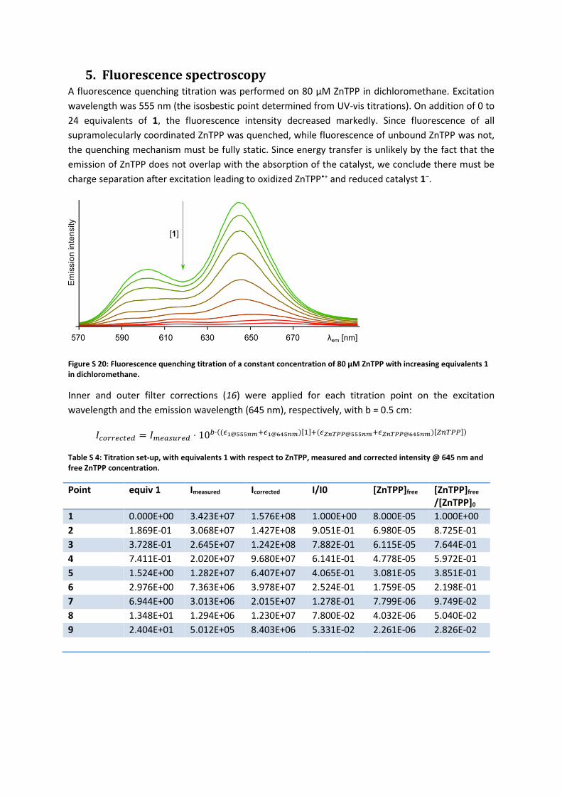
5. Fluorescence spectroscopy A fluorescence quenching titration was performed on 80 µM ZnTPP in dichloromethane. Excitation

wavelength was 555 nm (the isosbestic point determined from UV-vis titrations). On addition of 0 to

24 equivalents of 1, the fluorescence intensity decreased markedly. Since fluorescence of all

supramolecularly coordinated ZnTPP was quenched, while fluorescence of unbound ZnTPP was not,

the quenching mechanism must be fully static. Since energy transfer is unlikely by the fact that the

emission of ZnTPP does not overlap with the absorption of the catalyst, we conclude there must be

charge separation after excitation leading to oxidized ZnTPP•+ and reduced catalyst 1–.

Figure S 20: Fluorescence quenching titration of a constant concentration of 80 µM ZnTPP with increasing equivalents 1 in dichloromethane.

Inner and outer filter corrections (16) were applied for each titration point on the excitation

wavelength and the emission wavelength (645 nm), respectively, with b = 0.5 cm:

𝐼𝑐𝑜𝑟𝑟𝑒𝑐𝑡𝑒𝑑 = 𝐼𝑚𝑒𝑎𝑠𝑢𝑟𝑒𝑑 ⋅ 10𝑏⋅((𝜖1@555𝑛𝑚+𝜖1@645𝑛𝑚)[1]+(𝜖𝑍𝑛𝑇𝑃𝑃@555𝑛𝑚+𝜖𝑍𝑛𝑇𝑃𝑃@645𝑛𝑚)[𝑍𝑛𝑇𝑃𝑃])

Table S 4: Titration set-up, with equivalents 1 with respect to ZnTPP, measured and corrected intensity @ 645 nm and free ZnTPP concentration.

Point equiv 1 Imeasured Icorrected I/I0 [ZnTPP]free [ZnTPP]free /[ZnTPP]0

1 0.000E+00 3.423E+07 1.576E+08 1.000E+00 8.000E-05 1.000E+00

2 1.869E-01 3.068E+07 1.427E+08 9.051E-01 6.980E-05 8.725E-01

3 3.728E-01 2.645E+07 1.242E+08 7.882E-01 6.115E-05 7.644E-01

4 7.411E-01 2.020E+07 9.680E+07 6.141E-01 4.778E-05 5.972E-01

5 1.524E+00 1.282E+07 6.407E+07 4.065E-01 3.081E-05 3.851E-01

6 2.976E+00 7.363E+06 3.978E+07 2.524E-01 1.759E-05 2.198E-01

7 6.944E+00 3.013E+06 2.015E+07 1.278E-01 7.799E-06 9.749E-02

8 1.348E+01 1.294E+06 1.230E+07 7.800E-02 4.032E-06 5.040E-02

9 2.404E+01 5.012E+05 8.403E+06 5.331E-02 2.261E-06 2.826E-02

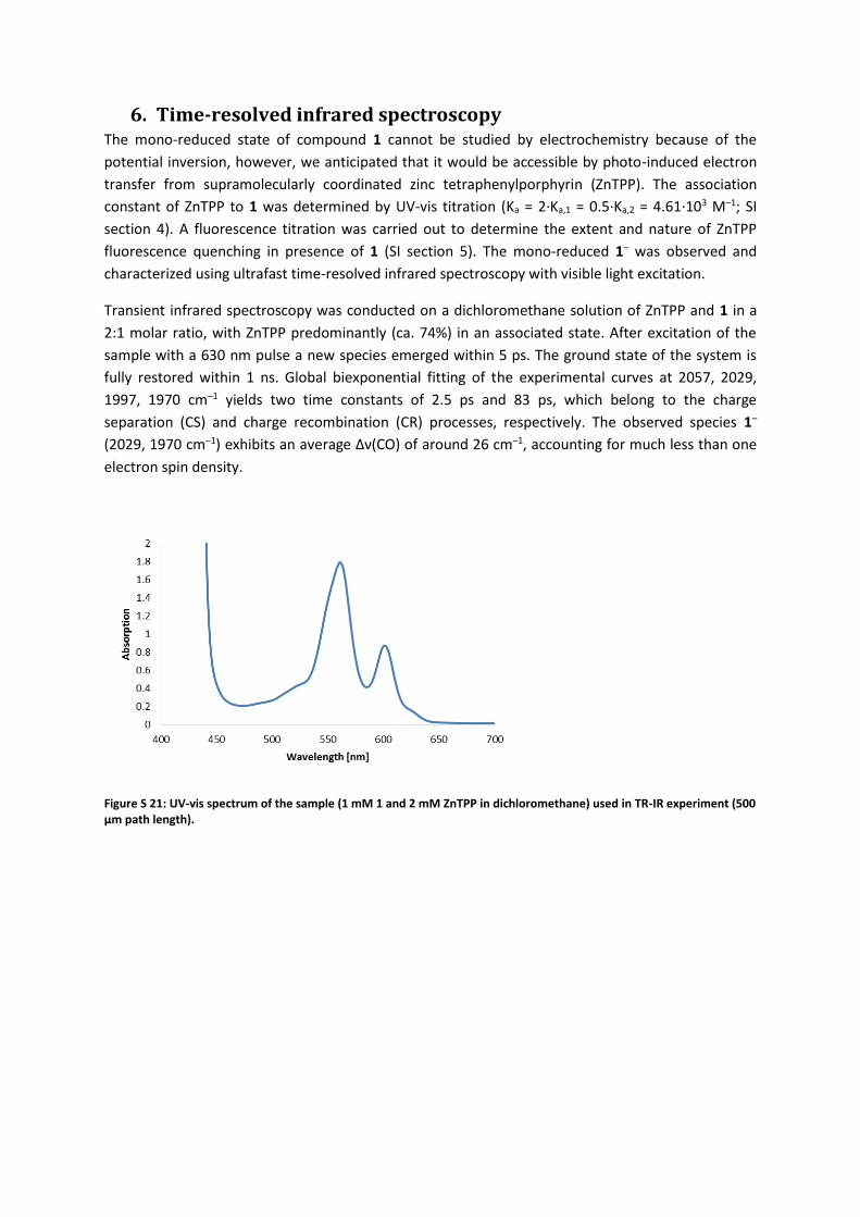
6. Time-resolved infrared spectroscopy The mono-reduced state of compound 1 cannot be studied by electrochemistry because of the

potential inversion, however, we anticipated that it would be accessible by photo-induced electron

transfer from supramolecularly coordinated zinc tetraphenylporphyrin (ZnTPP). The association

constant of ZnTPP to 1 was determined by UV-vis titration (Ka = 2·Ka,1 = 0.5·Ka,2 = 4.61·103 M–1; SI

section 4). A fluorescence titration was carried out to determine the extent and nature of ZnTPP

fluorescence quenching in presence of 1 (SI section 5). The mono-reduced 1– was observed and

characterized using ultrafast time-resolved infrared spectroscopy with visible light excitation.

Transient infrared spectroscopy was conducted on a dichloromethane solution of ZnTPP and 1 in a

2:1 molar ratio, with ZnTPP predominantly (ca. 74%) in an associated state. After excitation of the

sample with a 630 nm pulse a new species emerged within 5 ps. The ground state of the system is

fully restored within 1 ns. Global biexponential fitting of the experimental curves at 2057, 2029,

1997, 1970 cm–1 yields two time constants of 2.5 ps and 83 ps, which belong to the charge

separation (CS) and charge recombination (CR) processes, respectively. The observed species 1–

(2029, 1970 cm–1) exhibits an average Δν(CO) of around 26 cm–1, accounting for much less than one

electron spin density.

Figure S 21: UV-vis spectrum of the sample (1 mM 1 and 2 mM ZnTPP in dichloromethane) used in TR-IR experiment (500 µm path length).

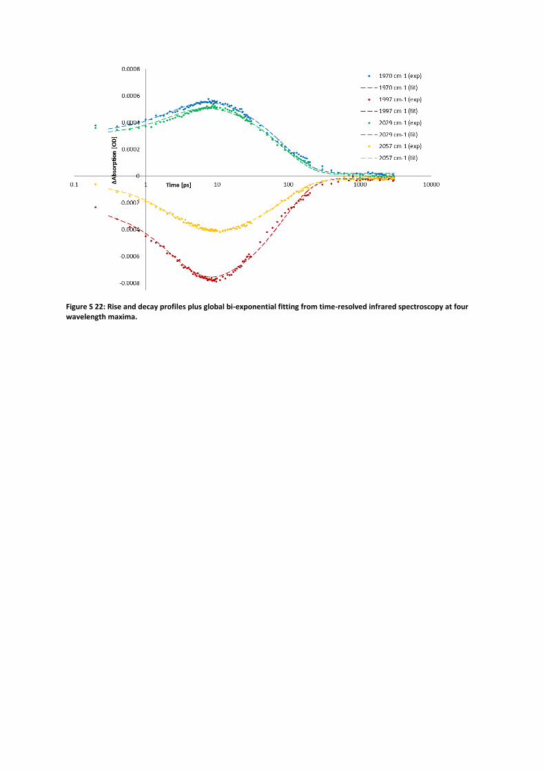
Figure S 22: Rise and decay profiles plus global bi-exponential fitting from time-resolved infrared spectroscopy at four wavelength maxima.

7. Electrochemistry of 1 in presence of acid

7.1 Cyclic voltammograms

Figure S 23: Cyclic voltammograms of 0.5 mM 1 and 4.0 mM Et3NHBF4 in dichloromethane containing 0.1 M TBAPF6 at varying scan speed.

Figure S 24: Cyclic voltammograms of 0.5 mM 1 and 8.0 mM Et3NHBF4 in dichloromethane containing 0.1 M TBAPF6 at varying scan speed.

Figure S 25: Cyclic voltammograms of 0.5 mM 1 and 16 mM Et3NHBF4 in dichloromethane containing 0.1 M TBAPF6 at varying scan speed.

Figure S 26: Cyclic voltammograms of 0.5 mM 1 and 32 mM Et3NHBF4 in dichloromethane containing 0.1 M TBAPF6 at varying scan speed.

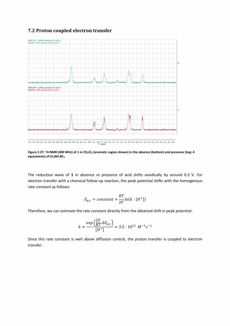
7.2 Proton coupled electron transfer

Figure S 27: 1H-NMR (400 MHz) of 1 in CD2Cl2 (aromatic region shown) in the absence (bottom) and presence (top; 4 equivalents) of Et3NH.BF4.

The reduction wave of 1 in absence vs presence of acid shifts anodically by around 0.3 V. For

electron transfer with a chemical follow-up reaction, the peak potential shifts with the homogenous

rate constant as follows:

𝐸𝑝,𝑐 = 𝑐𝑜𝑛𝑠𝑡𝑎𝑛𝑡 +𝑅𝑇

2𝐹ln(𝑘 ⋅ [𝐻+])

Therefore, we can estimate the rate constant directly from the obtained shift in peak potential:

𝑘 ≈exp (

2𝐹𝑅𝑇 𝛥𝐸𝑝,𝑐)

[𝐻+]≈ 3.5 ⋅ 1012 𝑀−1𝑠−1

Since this rate constant is well above diffusion control, the proton transfer is coupled to electron

transfer.

7.3 Determination of homogeneous and electrode mechanism

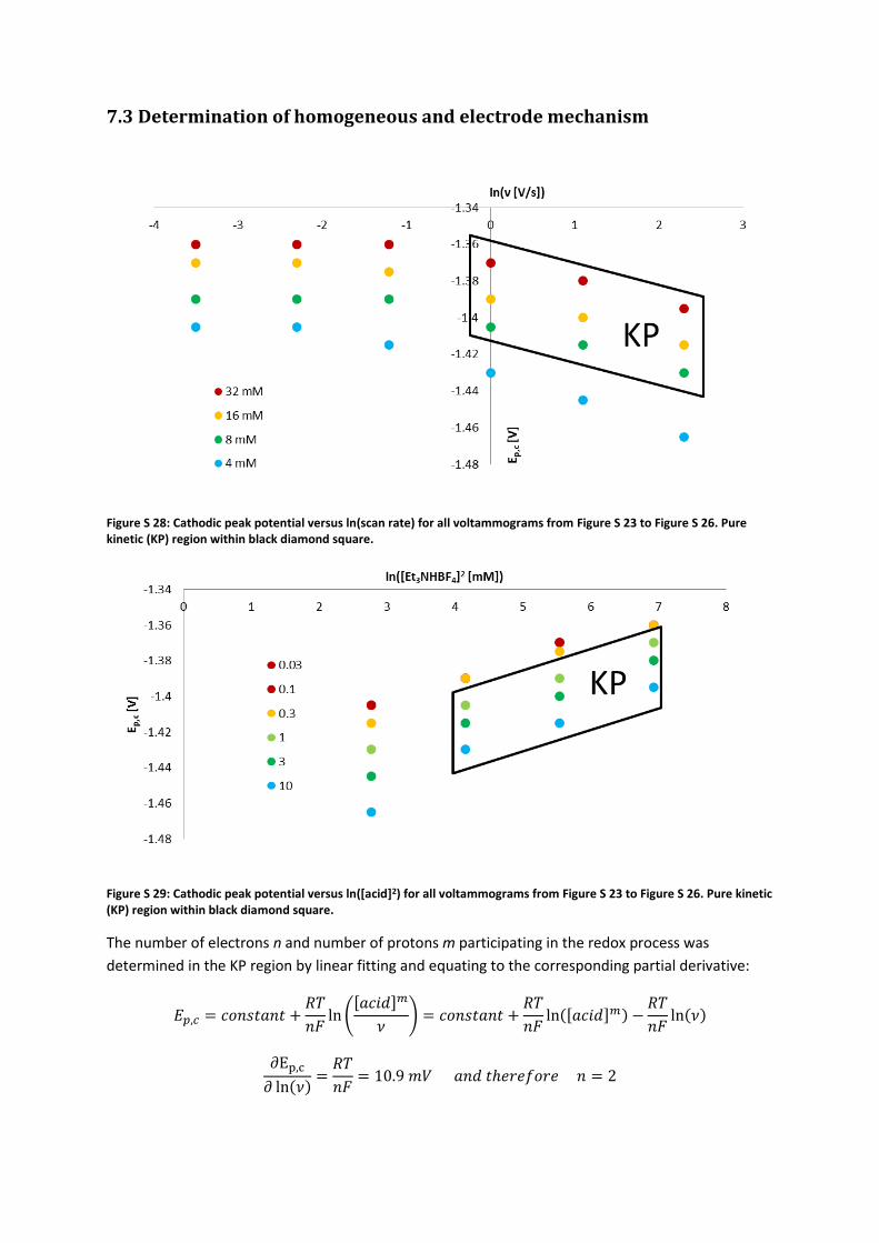
Figure S 28: Cathodic peak potential versus ln(scan rate) for all voltammograms from Figure S 23 to Figure S 26. Pure kinetic (KP) region within black diamond square.

Figure S 29: Cathodic peak potential versus ln([acid]2) for all voltammograms from Figure S 23 to Figure S 26. Pure kinetic (KP) region within black diamond square.

The number of electrons n and number of protons m participating in the redox process was

determined in the KP region by linear fitting and equating to the corresponding partial derivative:

𝐸𝑝,𝑐 = 𝑐𝑜𝑛𝑠𝑡𝑎𝑛𝑡 +𝑅𝑇

𝑛𝐹ln (

[𝑎𝑐𝑖𝑑]𝑚

𝜈) = 𝑐𝑜𝑛𝑠𝑡𝑎𝑛𝑡 +

𝑅𝑇

𝑛𝐹ln([𝑎𝑐𝑖𝑑]𝑚) −

𝑅𝑇

𝑛𝐹ln(𝜈)

∂Ep,c

𝜕 ln(𝜈)=

𝑅𝑇

𝑛𝐹= 10.9 𝑚𝑉 𝑎𝑛𝑑 𝑡ℎ𝑒𝑟𝑒𝑓𝑜𝑟𝑒 𝑛 = 2

∂Ep,c

𝜕 ln([𝑎𝑐𝑖𝑑])=

𝑅𝑇

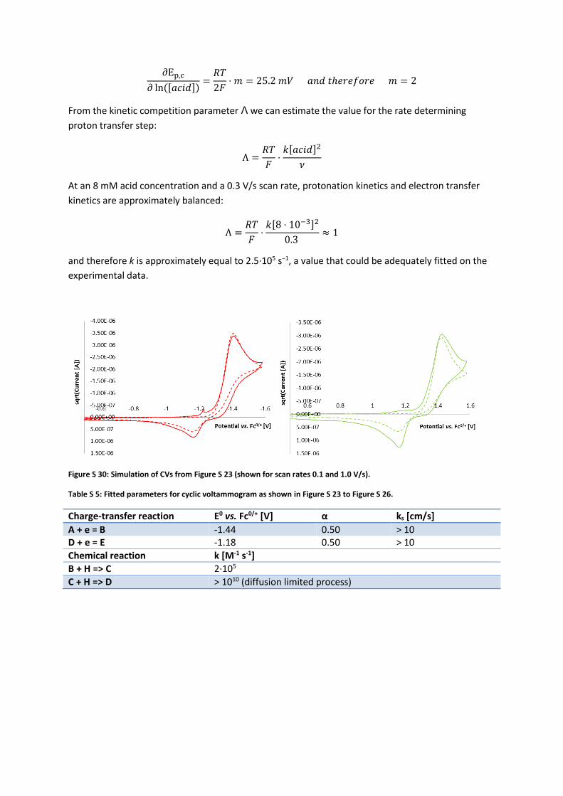
2𝐹⋅ 𝑚 = 25.2 𝑚𝑉 𝑎𝑛𝑑 𝑡ℎ𝑒𝑟𝑒𝑓𝑜𝑟𝑒 𝑚 = 2

From the kinetic competition parameter Λ we can estimate the value for the rate determining

proton transfer step:

Λ =𝑅𝑇

𝐹⋅

𝑘[𝑎𝑐𝑖𝑑]2

𝜈

At an 8 mM acid concentration and a 0.3 V/s scan rate, protonation kinetics and electron transfer

kinetics are approximately balanced:

Λ =𝑅𝑇

𝐹⋅

𝑘[8 ⋅ 10−3]2

0.3 ≈ 1

and therefore k is approximately equal to 2.5∙105 s−1, a value that could be adequately fitted on the

experimental data.

Figure S 30: Simulation of CVs from Figure S 23 (shown for scan rates 0.1 and 1.0 V/s).

Table S 5: Fitted parameters for cyclic voltammogram as shown in Figure S 23 to Figure S 26.

Charge-transfer reaction E0 vs. Fc0/+ [V] α ks [cm/s]

A + e = B -1.44 0.50 > 10 D + e = E -1.18 0.50 > 10

Chemical reaction k [M-1 s-1]

B + H => C 2∙105

C + H => D > 1010 (diffusion limited process)

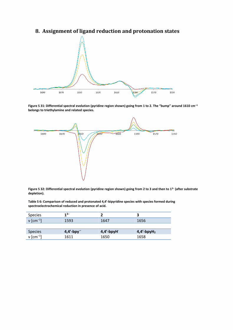
8. Assignment of ligand reduction and protonation states

Figure S 31: Differential spectral evolution (pyridine region shown) going from 1 to 2. The “bump” around 1610 cm–1 belongs to triethylamine and related species.

Figure S 32: Differential spectral evolution (pyridine region shown) going from 2 to 3 and then to 13– (after substrate depletion).

Table S 6: Comparison of reduced and protonated 4,4’-bipyridine species with species formed during spectroelectrochemical reduction in presence of acid.

Species 13– 2 3

ν [cm–1] 1593 1647 1656

Species 4,4’-bpy∙− 4,4’-bpyH∙ 4,4’-bpyH2 ν [cm–1] 1611 1650 1658

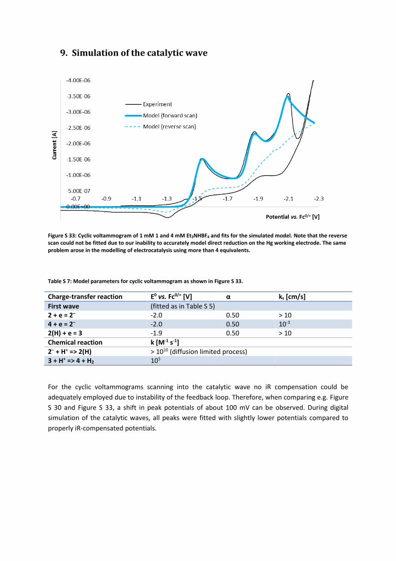
9. Simulation of the catalytic wave

Figure S 33: Cyclic voltammogram of 1 mM 1 and 4 mM Et3NHBF4 and fits for the simulated model. Note that the reverse scan could not be fitted due to our inability to accurately model direct reduction on the Hg working electrode. The same problem arose in the modelling of electrocatalysis using more than 4 equivalents.

Table S 7: Model parameters for cyclic voltammogram as shown in Figure S 33.

Charge-transfer reaction E0 vs. Fc0/+ [V] α ks [cm/s]

First wave (fitted as in Table S 5) 2 + e = 2– -2.0 0.50 > 10 4 + e = 2– -2.0 0.50 10-3 2(H) + e = 3 -1.9 0.50 > 10

Chemical reaction k [M-1 s-1]

2– + H+ => 2(H) > 1010 (diffusion limited process) 3 + H+ => 4 + H2 105

For the cyclic voltammograms scanning into the catalytic wave no iR compensation could be

adequately employed due to instability of the feedback loop. Therefore, when comparing e.g. Figure

S 30 and Figure S 33, a shift in peak potentials of about 100 mV can be observed. During digital

simulation of the catalytic waves, all peaks were fitted with slightly lower potentials compared to

properly iR-compensated potentials.

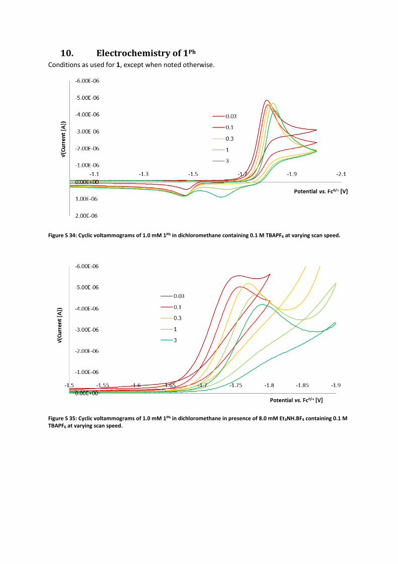
10. Electrochemistry of 1Ph Conditions as used for 1, except when noted otherwise.

Figure S 34: Cyclic voltammograms of 1.0 mM 1Ph in dichloromethane containing 0.1 M TBAPF6 at varying scan speed.

Figure S 35: Cyclic voltammograms of 1.0 mM 1Ph in dichloromethane in presence of 8.0 mM Et3NH.BF4 containing 0.1 M TBAPF6 at varying scan speed.

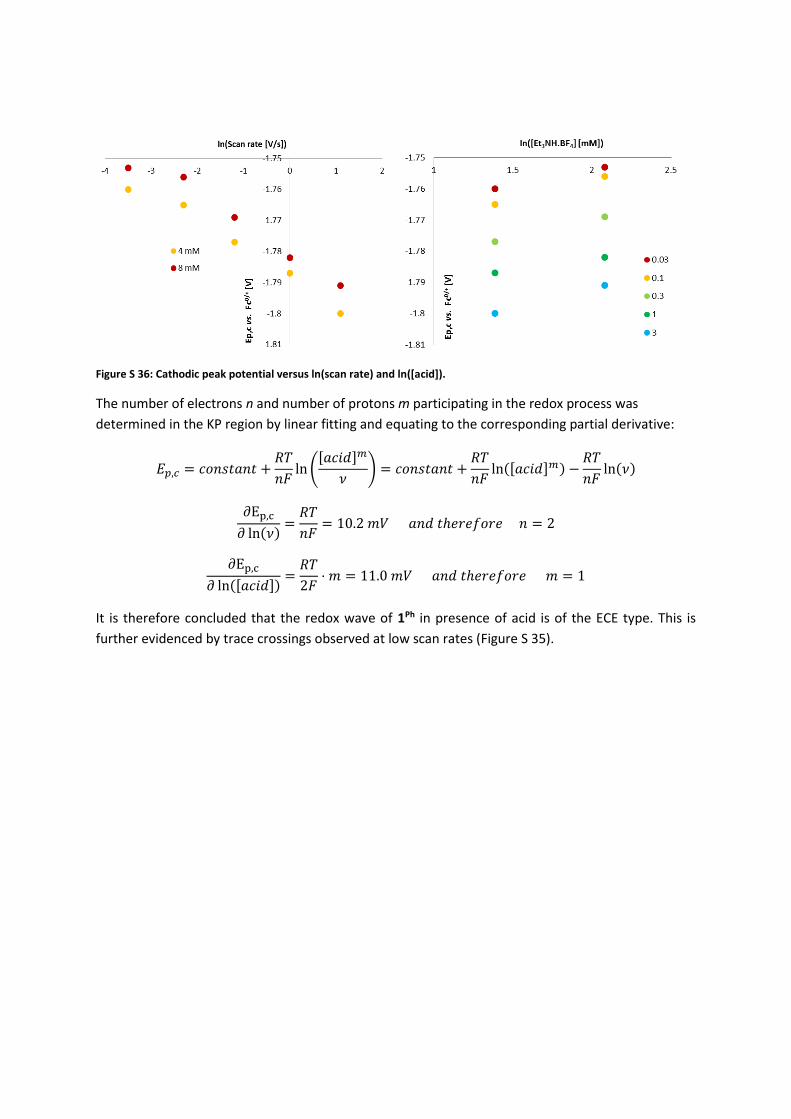
Figure S 36: Cathodic peak potential versus ln(scan rate) and ln([acid]).

The number of electrons n and number of protons m participating in the redox process was

determined in the KP region by linear fitting and equating to the corresponding partial derivative:

𝐸𝑝,𝑐 = 𝑐𝑜𝑛𝑠𝑡𝑎𝑛𝑡 +𝑅𝑇

𝑛𝐹ln (

[𝑎𝑐𝑖𝑑]𝑚

𝜈) = 𝑐𝑜𝑛𝑠𝑡𝑎𝑛𝑡 +

𝑅𝑇

𝑛𝐹ln([𝑎𝑐𝑖𝑑]𝑚) −

𝑅𝑇

𝑛𝐹ln(𝜈)

∂Ep,c

𝜕 ln(𝜈)=

𝑅𝑇

𝑛𝐹= 10.2 𝑚𝑉 𝑎𝑛𝑑 𝑡ℎ𝑒𝑟𝑒𝑓𝑜𝑟𝑒 𝑛 = 2

∂Ep,c

𝜕 ln([𝑎𝑐𝑖𝑑])=

𝑅𝑇

2𝐹⋅ 𝑚 = 11.0 𝑚𝑉 𝑎𝑛𝑑 𝑡ℎ𝑒𝑟𝑒𝑓𝑜𝑟𝑒 𝑚 = 1

It is therefore concluded that the redox wave of 1Ph in presence of acid is of the ECE type. This is

further evidenced by trace crossings observed at low scan rates (Figure S 35).

11. Electrochemistry in aqueous acid

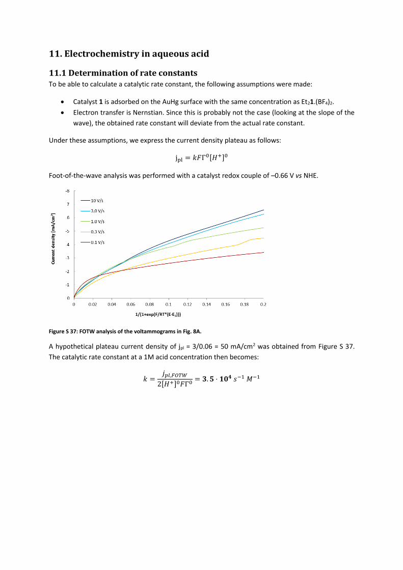
11.1 Determination of rate constants To be able to calculate a catalytic rate constant, the following assumptions were made:

Catalyst 1 is adsorbed on the AuHg surface with the same concentration as Et21.(BF4)2.

Electron transfer is Nernstian. Since this is probably not the case (looking at the slope of the

wave), the obtained rate constant will deviate from the actual rate constant.

Under these assumptions, we express the current density plateau as follows:

jpl = 𝑘𝐹Γ0[𝐻+]0

Foot-of-the-wave analysis was performed with a catalyst redox couple of –0.66 V vs NHE.

Figure S 37: FOTW analysis of the voltammograms in Fig. 8A.

A hypothetical plateau current density of jpl = 3/0.06 = 50 mA/cm2 was obtained from Figure S 37.

The catalytic rate constant at a 1M acid concentration then becomes:

𝑘 =𝑗𝑝𝑙,𝐹𝑂𝑇𝑊

2[𝐻+]0𝐹Γ0= 𝟑. 𝟓 ⋅ 𝟏𝟎𝟒 𝑠−1 𝑀−1

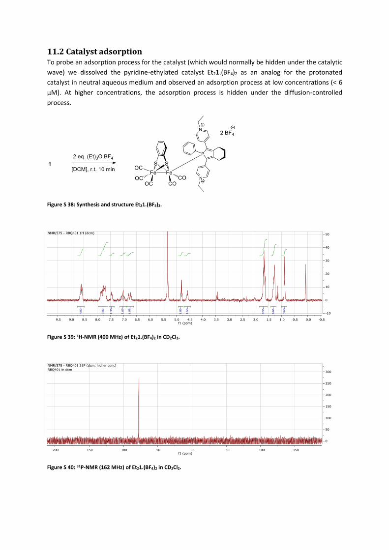
11.2 Catalyst adsorption To probe an adsorption process for the catalyst (which would normally be hidden under the catalytic

wave) we dissolved the pyridine-ethylated catalyst Et21.(BF4)2 as an analog for the protonated

catalyst in neutral aqueous medium and observed an adsorption process at low concentrations (< 6

μM). At higher concentrations, the adsorption process is hidden under the diffusion-controlled

process.

Figure S 38: Synthesis and structure Et21.(BF4)2.

Figure S 39: 1H-NMR (400 MHz) of Et21.(BF4)2 in CD2Cl2.

Figure S 40: 31P-NMR (162 MHz) of Et21.(BF4)2 in CD2Cl2.

Figure S 41: Cyclic voltammograms of 2 μM Et21.(BF4)2 in 0.1M Na2SO4.

Figure S 42: Peak current vs. scan rate for the adsorption waves in Figure S 41.

From the slope in Figure S 42, a surface concentration Γ0 of 7.3∙10−12 mol/cm2 (two-electron process)

was obtained through Γ0 =𝜕𝑖𝑝

𝜕𝜈

1

9.40⋅105𝑆𝑛2.

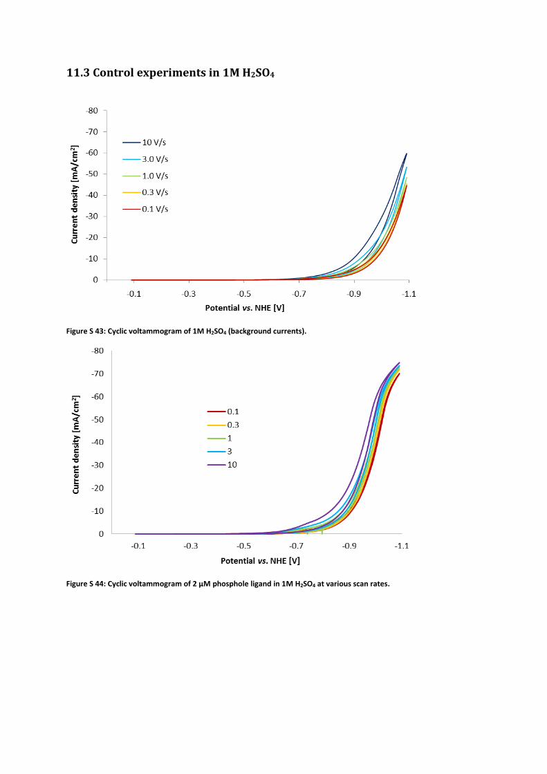
11.3 Control experiments in 1M H2SO4

Figure S 43: Cyclic voltammogram of 1M H2SO4 (background currents).

Figure S 44: Cyclic voltammogram of 2 μM phosphole ligand in 1M H2SO4 at various scan rates.

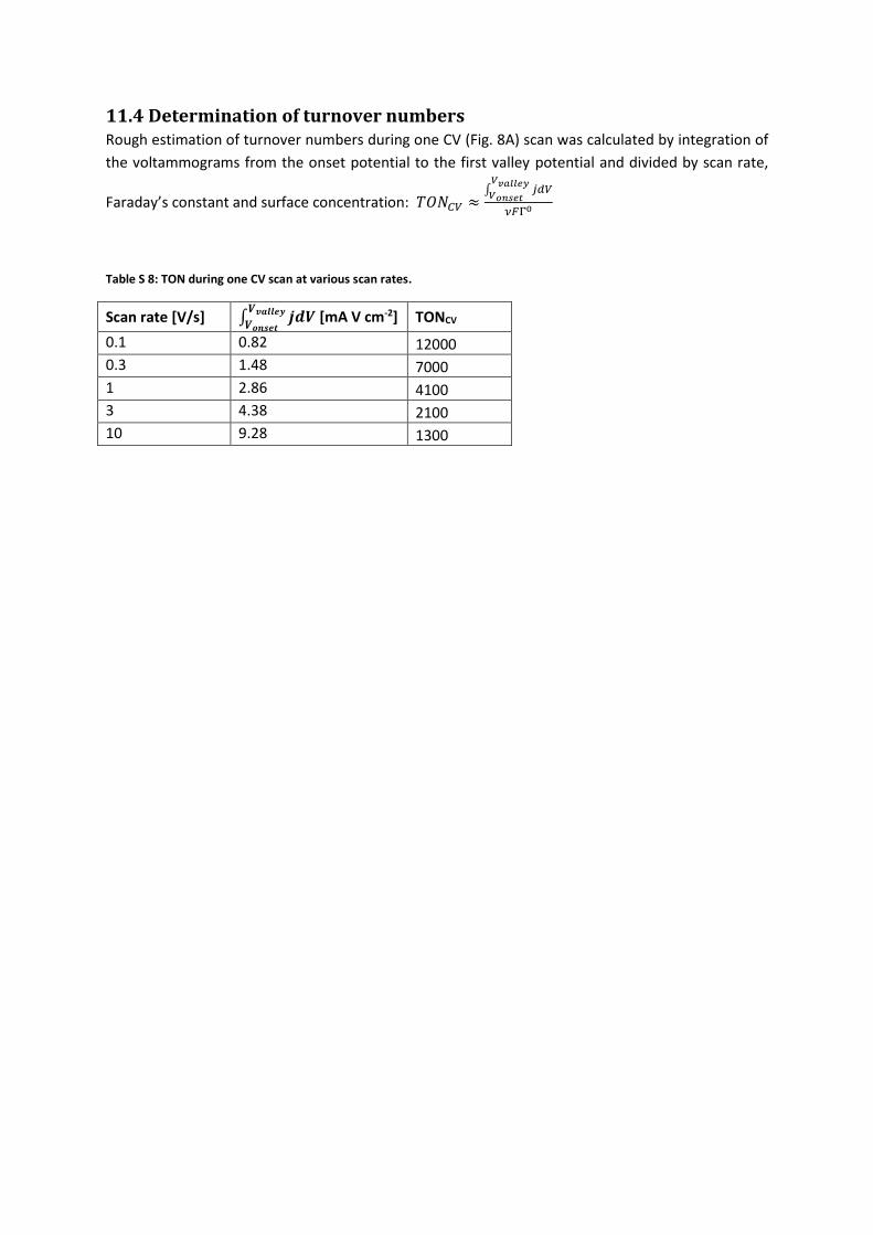
11.4 Determination of turnover numbers Rough estimation of turnover numbers during one CV (Fig. 8A) scan was calculated by integration of

the voltammograms from the onset potential to the first valley potential and divided by scan rate,

Faraday’s constant and surface concentration: 𝑇𝑂𝑁𝐶𝑉 ≈∫ 𝑗𝑑𝑉

𝑉𝑣𝑎𝑙𝑙𝑒𝑦

𝑉𝑜𝑛𝑠𝑒𝑡

𝜈𝐹Γ0

Table S 8: TON during one CV scan at various scan rates.

Scan rate [V/s] ∫ 𝒋𝒅𝑽𝑽𝒗𝒂𝒍𝒍𝒆𝒚

𝑽𝒐𝒏𝒔𝒆𝒕 [mA V cm-2] TONCV

0.1 0.82 12000

0.3 1.48 7000

1 2.86 4100

3 4.38 2100

10 9.28 1300