Supplementary Figure 1: TOAS data analysis fit

2-component fit

3-component fit

Supplementary Figure 1: TOAS data, fit and residual from a global analysis using either 2 or

3 exponential components.

Supplementary Figure 2: TOAS data analysis results

Supplementary Figure 2: Probability distributions of the time constants 1 (left) and 2 (right)

extracted from the global analysis of data recorded at different excitation wavelengths.

Supplementary Figure 3: XES data extraction and reduction

Supplementary Figure 3: (A) Flowchart of the XES data extraction-correction process. (B)

Processing of an XES kinetic-scan: (Left) Sum of the read-out values (ROVs) for each pixel

after read-out (step 1), (Middle) Summed ROVs after detector corrections, (step 2), (Right)

Summed photon counting events for each pixel after single-photon discrimination (step 3).

Some of the data had to be discarded due to high read-out noise, resulting in the empty section

on the right panel. (C) Single-pixel histogram of a strongly illuminated pixel after step 1 and

2. The peak at ROV = 0 corresponds to readout of the pixel after no photons were detected,

the peak at ROV = 100 corresponds to 1-photon counting events, while the clustering of

counts observed around ROV = 210 originates from 2-photon events.

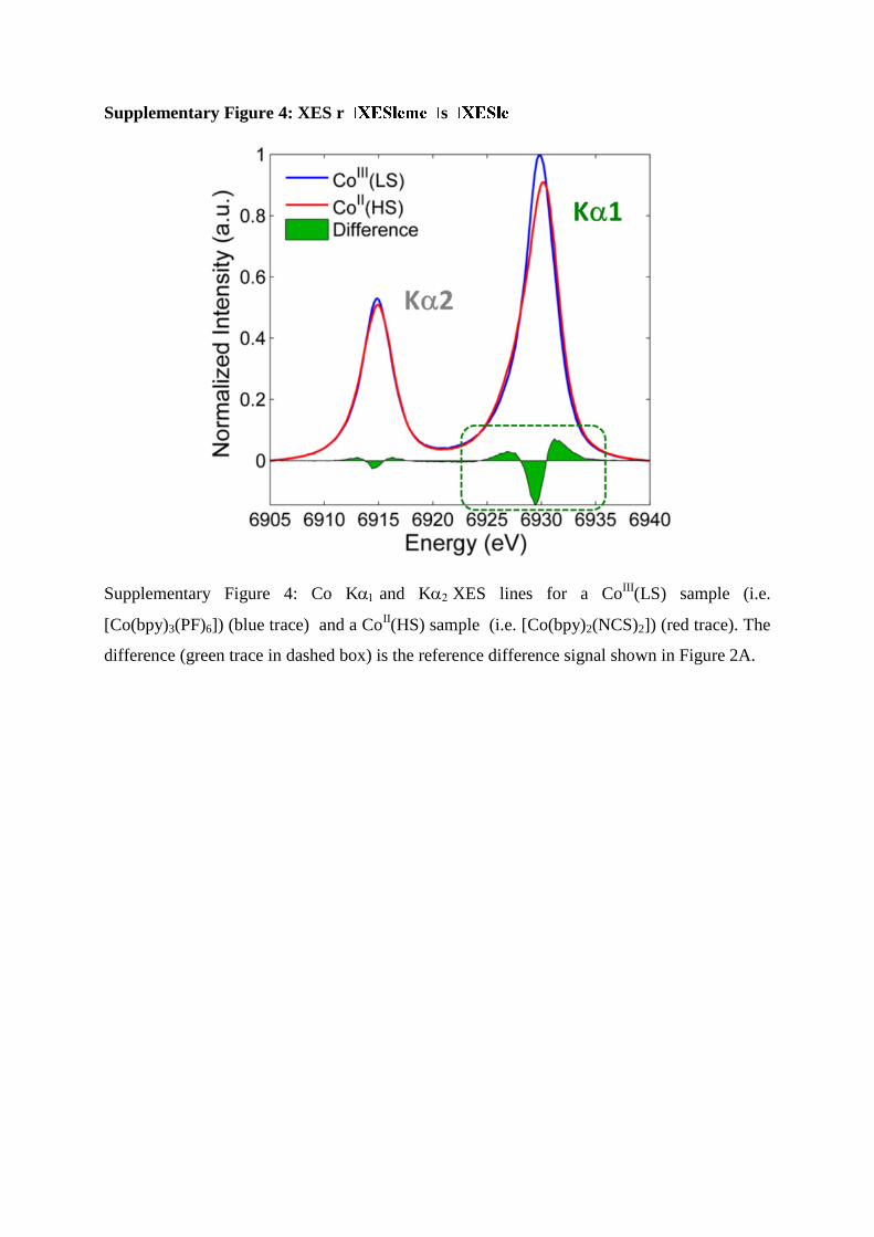
Supplementary Figure 4: XES r s

Supplementary Figure 4: Co Kand KXES lines for a CoIII

(LS) sample (i.e.

[Co(bpy)3(PF)6]) (blue trace) and a CoII(HS) sample (i.e. [Co(bpy)2(NCS)2]) (red trace). The

difference (green trace in dashed box) is the reference difference signal shown in Figure 2A.

Supplementary Figure 5: Comparison between XES fitting models

Supplementary Figure 5: The resulting fits to the data of models A (cyan) and B (blue).

Supplementary Figure 6: SVD-based background-removal of XDS data.

Supplementary Figure 6: SXDS(Q,t) data before (left) and after (right) the SVD-based

background-removal procedure. The black box on the left panel shows the subset of data used

to construct the SVD components.

Supplementary Figure 7: XDS sample reference signal

Supplementary Figure 7: Ssolute(Q) resulting from a [1Ru

II=

1Co

III(LS)] to [

2Ru

III=

4Co

II(HS)]

conversion.

Supplementary Figure 8: XDS solvent reference signal

Supplementary Figure 8: The effect of the X-ray source energy spectrum on the temperature

solvent differential (TSD). (A) Experimental TSD obtained at ID09b (black) and noise-

reduced profile (red). (B) A “monochromatic” TSD (blue) was obtained by deconvoluting the

noise-reduced profile (red) by the energy spectrum of the ID09 multilayer optics. This

simulated “monochromatic” curve was then convoluted with the energy spectrum of the

XFEL source (green) and with the U17 pink beam at ID09 (black) for comparion. The traces

are vertically offset for clarity.

Supplementary Figure 9: Pairwise radial distribution functions of acetonitrile

Supplementary Figure 9: Pairwise radial distribution functions o for the constituent

components of acetonitrile.

Supplementary Figure 10: Dependency of the simulated XDS signal on the Co-N bond

length elongation

Supplementary Figure 10: Simulated SXDS(Q) curves for the structural transition from

[1Ru

II=

1Co

III] to [

2Ru

III=

4Co

II], where the Co-N bond length elongation – ΔR(Co-N) – has

been varied between 0.15Å and 0.25 Å. The left panel shows the curves on an absolute scale,

the right panel shows the same data normalized to the signal amplitude.

Supplementary Figure 11: Dependency of the simulated XDS signal on the Co-N bond

length elongation

Supplementary Figure 11: (A). Thermal distribution of individual Co-N bond lengths for (a)

the [1Ru

II=

1Co

III(LS)] ground state and (b) the [

2Ru

III=

4Co

II(HS)] charge separated state,

where the CoII center is in the HS state. (B) Thermal distribution of average Co-N bond

lengths for the [1Ru

II=

1Co

III(LS)] ground state and the [

2Ru

III=

4Co

II(HS)] charge separated

state, where the CoII center is in the HS state.

Supplementary Note 1: TOAS data analysis

The TOAS data were fitted within a standard global analysis framework.1 The number of

required decay associated spectra (DAS) can be estimated by inspection of the residuals, as

shown in Supplementary Figure 1.

With a two-component fit, the best results are obtained with one sub picosecond and one

nanosecond component (i.e. without the vibrational cooling). There is clear structure in the

residual of these two-component fit showing that a three-component model (and thus the

effects of vibrational cooling) is required to describe the data. The derived time constants are

all dependent on the excitation wavelength. This is illustrated for three different excitation

wavelengths (400, 440 and 480 nm) in Supplementary Figure 2.

Supplementary Note 2: XES data extraction and reduction

The low readout noise of the MPCCD detector allowed explicit single-photon discrimination

of the XES signal. A flow-chart of the data extraction-correction process is shown in

Supplementary Figure 3A.

Step 1: Readout

The MPCCD detector is read out as a 2D image containing the read-out value

(ROV) of each pixel.

Step 2: Pedestal and common-mode detector corrections

The so-called “pedestal” correction ensures that the zero-photon ROVs of all the

pixels are close to 0 analogue-to-digital units (ADU). A set of 15000 dark-measurements (i.e.

images with the X-rays shutter closed and no X-rays hitting the detector) was averaged,

yielding the average 0-photon signal level for each pixel. This background was subtracted

from all further images. Three sets of such dark-measurements were recorded in the course of

the experimental run in order to confirm that this background did not change over time.

Common-mode artefacts arising from amplifier/current supply electronics were negligible.

Step 3: Calibration and scaling (pixel-based gainmap and single photon discrimination)

A pixel-specific gainmap constructed from single-pixel ROVs was applied. A typical

histogram of the ROVs for a pixel seeing seeing a high photon intensity is plotted in

Supplementary Figure 3C (blue line), the inset shows a zoom-in.

The peaks centered at ROV= 0 ADU, at ROV= 100 ADU and the clustering of counts around

210 ADU correspond to 0-, 1- and 2-photon counting events respectively. For each X-ray

illuminated pixel, Gaussian functions of RMS were fitted to the 0-photon signal (red line),

and the 1-photon signals (cyan line) individually. The single-pixel gainmap was constructed

by defining the center peak positions of the two Gaussians to 0 and 1 respectively. As can be

seen from the inset in Supplementary Figure 3C, many ROVs fall between the 0- and 1-

photon peaks. This interval is assigned to fractional photon events. The most robust approach

to account for them was to define the number of detected 1-photon and 2-photon events in an

exposed image as the number of pixels for which the single-pixel gain-corrected ROVs were

such that 0.5<ROV<1.5 and ROV>1.5 respectively. Since the maximum count rate of any

pixel was ~0.025 ph/exposure, gain-corrected ROVs corresponding to 3 or more photons were

not considered. A lower threshold of 9σ of the zero-photon readout was enforced in the

single-photon discrimination to remove false counting events from the readout noise.

Supplementary Figure 3B follows a detector image across the 3 stages of the data extraction-

correction procedure. Note that the high read-out noise of the third detector from the top made

explicit single-photon counting in this element impossible, resulting in the absence of data in

the corresponding panel of Supplementary Figure 3B. Even though this approach discards all

photons hitting 1/3 of active area of the detector, it resulted in the best signal to noise ratio,

with the mean standard deviation of each data point typically being within 30% of that

expected from a true Poisson distribution. The final signal strength obtained in the Co Kα1

emission peak is the sum of all the detector counts for a given pulse and was typically ~20

photons/pulse, while the background count was ~0.2 photons/pulse.

Supplementary Note 3: XES data analysis

The K spectra originate from multiplet and spin orbit interactions. In

transition metal systems, it is highly sensitive to the oxidation state and to the number of

unpaired electrons. A frequent evaluation approach that is applicable to the interpretation of

photoinduced transient K2p1s and K 3p1s spectra is based on constructing

differences of steady-state spectra from suitable reference complexes; the integrals of the

absolute values of the difference spectra are then proportional to the conversion yield. This

approach is somewhat similar to the treatment of X-ray dichroism, although sum rules do not

apply, and one needs to find acceptable reference compounds.2

Still, this approach is

quantitative for two-state transitions,3 and can be indicative of more complex spin-state

transitions, as demonstrated in numerous studies4,5,6,7,8,9,10,11,12

However, in the experiments reported in this work, the short effective data

collection time did not permit to obtain a sufficiently large set of spectra with clear references

and good statistics to fully exploit this approach. It was nevertheless indirectly applied to

follow the spectral variations, since for the Kspectra, the linewidth (full-width at half-

maximum FWHM) can also be exploited to calibrate the spin momentum on the cobalt center.

Although the 2p-3d exchange interaction is rather small, its variation upon increase in spin-

state appears as a clear broadening2. After a careful comparison with the static lineshapes

obtained at the ID26 beamline of the ESRF (shown in Supplementary Figure 4), we can

determine that the 0.6 eV FWHM difference observed in the current experiment for the

ground and photoexcited state corresponds to a spin-state change of S=1.5 at t=20 ps. Since

the initial spin momentum of the 1Co

III is S=0, this corresponds to S=3/2, a spin-state HS of

4Co

II. Given that the total integrated Kα1 emission intensity does not depend upon the charge

and spin-state2 the relative changes in the FWHM of the emission line for the different Co

species directly result in an inverse lowering of the maximum emission intensity, i.e. the peak

height. This is the parameter measured and plotted in the kinetic traces presented in the main

text.

Supplementary Note 4: Computational details for the DFT optimization

All the calculations were carried out with the ORCA program package.13,14

The geometries of

[1Ru

III(=)

1Co

III (LS)], [

2Ru

III(=)

4Co

II (HS)] and [

2Ru

III(=)

4Co

II (HS)] were fully optimized

with the B3LYP*15

/TZVP method. This functional has provided reasonable results for the

structures and energetics of the LS and HS states of transition metal complexes.16,17,18,19,20

The

conducting-like screening solvation model (COSMO)21

was applied with ε = 36.6 as

appropriate dielectric constant for acetonitrile. The Kohn-Sham orbitals were extracted from

the converged wave functions corresponding to single point calculations performed at the

optimized geometries.

Supplementary Note 5: XDS Data Analysis - Construction of the XDS difference signals,

SXDS(Q,t)

The 2D X-ray Diffuse Scattering (XDS) images extracted from the MPCCD detector were

corrected to account for the effects of:

1) the X-ray beam polarization,

2) the X-ray absorption of 8 keV photons throughout the liquid sheet ,

3) the solid angle subtended by each detector pixel,

4) the X-ray absorption probability of an 8 keV photon within a pixel.

The resulting images were then integrated azimuthally around the beam center (found by

circle-fits to the liquid-peak in the 2D images) producing 1D curves of the scattering intensity

S(Q), where

2sin4Q is the momentum transfer, 2θ is the scattering angle, and λ is the

X-ray wavelength. The first step in the analysis of S(Q) was a simple filtering procedure. Any

exposure where either I0 (the incident intensity) or I (the integrated intensity on the MPCCD)

fell outside one standard deviation from the mean of either of the two intensities was

discarded. The remaining SXDS(Q,t) were averaged for each time-delay and scaled to a

simulated scattering curve SSim(Q) = SCoh(Q) + SIncoh(Q), which is the sum of the coherent

SCoh(Q) and incoherent SIncoh(Q) scattering arising from a “Liquid Unit Cell”, L.U.C, i.e. an

ensemble of molecules representing the stoichiometry of the sample. In the present case, the

L.U.C consisted of a single RuII=

1Co

III molecule, 5 PF6

- ions and 19.15 M/6 mM = 3191

acetonitrile molecules. SCoh(Q) was calculated from the orientation-averaged Debye equation

by using the isolated-atom formalism. The atomic form factors were described by the Cromer-

Mann parameterization22

. SIncoh(Q) was obtained from the parameterization provided by

Hajdu23

. Scaling S(Q,t) to the L.U.C. Ssim(Q) was done by minimizing [SSim(Q) – · SXDS(Q,t)]

for 1.5 Å-1

<Q< 1.8 Å-1

around a nodal point in the difference scattering signal24

. This step

effectively put the SXDS(Q,t) on an absolute scale of electron units/LUC25

. The XDS difference

signals SXDS(Q,t) were calculated for each t by subtracting the average signal recorded for

the unpumped sample OffQStQStQS XDSXDSXDS )(),(),( , where SXDS(Q)Off is defined as the

mean of the earliest 12 time-delays for which the X-ray pulses arrived from 12 ps to 45 ps

before the laser pulse, namely 12),()(11

1

iiXDSOffXDS tQSQS

Supplementary Note 6: XDS Data Analysis - SVD-based background contributions to

SXDS(Q,t)

The XDS difference signals SXDS(Q,t) obtained for t<0 contain a considerable amount of

noise. If the background contributions were constant during acquisition, these SXDS(Q,t)

should in principle amount to statistical fluctuations. In order to identify and remove these

contributions, Singular Value Decomposition (SVD) was applied to the set of SXDS(Q,t)

curves calculated in the region used to construct SXDS(Q)Off. In general, SVD analysis

decomposes any matrix X as the product X = U*S*VT, where U and V are unitary matrices,

while S is a diagonal matrix. Taking X as the data matrix, the columns of U are the singular

vectors representing the variation in the data matrix X along the time coordinate, and V

contains the time-dependency of this variation. The elements of the diagonal matrix S denote

the relative magnitudes of the singular vectors. Inspection of S indicates that five singular

vectors are sufficient to accurately represent the variation in the SXDS(Q)Off data matrix, as the

singular values Sii for i > 5 become very small. The residual signal SXDS(Q, t)res = |SXDS(Q,t)

- i·Sii·Uji | for each t as a function of the 5 scaling parameters 1-5 is shown in

Supplementary Figure 6. A 10 point smoothing was applied to the individual traces, followed

by a 3x3 point median filtering. For all time delays, the fluctuating background can therefore

be accurately described by a sum of five singular vectors such that ΔSXDS(Q,t)back =

51

)()(i

SVD

ii QSt , where ijiii USQS SVD )( . Observing that this background-removal

procedure reduced the subset of data for t < 0 to a negligible level validated the use of the

SVD-determined descriptor vectors in an unconstrained fit of the SXDS(Q,t). The

implementation of this methodology in the full global-fit analysis is described in the next

section.

Supplementary Note 7: XDS Data Analysis - Sample contributions to SXDS(Q,t)

The SXDS(Q,t) contains contributions from all the structural changes that occur in the probed

sample volume upon laser excitation. It is usually expressed as the sum of 3 terms:

i) The solute termSsolute(Q,t), arising from structural changes in the solute

ii) The solvent term Ssolvent(Q,t), arising from structural changes of the bulk solvent

iii) The solute-solvent cross-term, arising from structural changes of the solvent-shell

surrounding the solute.

The solute term

This term was estimated from the molecular geometries of the [1Ru

II=

1Co

III(LS)] and

[2Ru

III=

4Co

II(HS)] optimized through DFT using the ORCA 2.8 program package

13 with the

BP8626,27

gradient-corrected (GGA) exchange-correlation functional and Gaussian type TZVP

basis set. The conducting-like screening solvation model (COSMO)21

was applied with ε =

36.6 as appropriate dielectric constant for acetonitrile. The coherent scattering of these two

structures was then simulated by employing the orientation-averaged Debye equation (the

incoherent scattering was discarded since it does not depend on the molecular structure).

Supplementary Figure 7 shows the simulated SXDS(Q) obtained from subtracting the two

patterns.

From these considerations, the solute term was expressed as )(),( QSttQS solutesolute ,

where γ(t) is the time-dependent excitation fraction of [2Ru

III=

4Co

II(HS)].

The solvent term

Assuming the validity of a classical continuum description, the equilibrated state of the

solvent can be expressed as a function of two independent hydrodynamical variables chosen

as the temperature (T) and the density (). The Ssolvent that originates from the bulk-solvent

response can be described in terms of their elementary variations ΔT(t) and Δρ(t). Numerous

investigations at synchrotron sources have demonstrated that a first order treatment is

adequate to model the response on the hundreds of picoseconds to hundreds of milliseconds

time scales. Within this framework the solvent term is quantified through the following linear

combination:

T

solvent

QSt

T

TQStTtQS

),()(

),()(),( (Supplementary Equation 1)

where T

TQS

),( and T

QS

),( are the difference scattering signals arising from a change in T at

constant and from a change in at constant T, respectively. These studies have also shown

that T

TQS

),(and

T

QS

),( can be measured independently, making it possible to extract

ΔT(t) and Δρ(t) directly from the transient Ssolvent signals. Simple arguments allow

determining the time scales on which the various contributions play a role. Considering first

Δρ(t), it has been shown24

that for times t such that t < d/vs, where d is the FWHM of the laser

spot and vs is the speed of sound in the liquid, no thermal expansion of the solvent has yet

taken place. With the present experimental conditions (d =500 µm FWHM and vs=1280 m/s

for MeCN), thermal expansion is expected to happen on the 400 ns time scale, which is

beyond the temporal window probed, so that Ssolvent reduces to the contribution from

impulsive solvent heating :

T

QStTtQsolventS

)()(),( . The reference difference scattering signal,

T

QS

)( (called the

temperature solvent differential (TSD)) was acquired independently during a dedicated study

at ID09b, ESRF28

. The data were measured using multilayer optics characterized by a 2.5%

bandwidth (bw). Since this is broader than the intrinsic 0.3% bw of the XFEL beam, the

influence of the X-ray source spectrum had to be investigated. As a first step, a TSD that

would be obtained from a monochromatic beam was constructed from the measurement in ref

28 shown in Supplementary Figure 8A (black trace) after standard filtering (red trace), as

described in ref 18. Supplementary Figure 8B shows the resulting curve after Gaussian

deconvolution (blue trace). This “monochromatic” TSD (blue) was convoluted with the 2.5%

bw of the multilayer (red) and the intrinsic 0.3% bw of an XFEL beam (green). The three

curves are indistinguishable, demonstrating that the ID09b reference can be introduced in the

analysis of the difference scattering signal from XFEL sources. The convolution of the

simulated monochromatic TSD with the full spectrum of the U17 undulator at ID09b (‘pink’

beam) is included for comparison (black trace).

SXDS(Q,t) from the sample

Summarizing the previous sections, Ssample could be expressed as:

T

QStTQSttQS solutesample

)()(, (Supplementary Equation 2)

where t is the fraction of charge-separated molecules, )(QSsolute is the difference

between the signal simulated for the RuII=

1Co

III(LS) and Ru

III=

4Co

II(HS) DFT structures,

tT is the change in temperature and T

QS

)( is the change in scattering signal caused by an

increase of MeCN temperature at constant density.

Supplementary Note 8: XDS Data Analysis - Fit-based analysis of SXDS(Q,t)

Following the methodology presented by Haldrup29

, each individual difference

scattering signal SXDS(Q,t) was expressed as a sum of a background contribution (ΔSback(Q,t)

=

51

)()(

i

SVDi

i QSt ) and a term ΔSsample(Q,t) from sample structural changes, both introduced

above. For each time delay, the residual function:

)1/(),(

)()(),(),(

2

2

51

.

pNtQ

QSttQStQS

S

XDS

i

SVDi

isample

res

(Supplementary Equation 3)

was minimized. The denominator )1/(),(2 pNtQXDS incorporates the point-to-point

difference signal noise XDS(Q,t)25

, as well as the number of data points N, and the number of

free parameters p in the fit. As such, Sres can be directly interpreted as a 2 estimator. This

allowed extracting the absolute magnitude of every SVD scaling parameters αi(t), for each

time point. While the average value for two of the αi(t) parameters changed gradually over the

duration of the scan, no systematic evolution was observed around or after t = 0. Explicit

inclusion of a density term Ssolvent returned Δρ(t) ≈ 0 for all time delays recorded. Any

contribution of the solute-solvent cross-term to SXDS(Q,t) was below the detection threshold.

Supplementary Note 9: XDS Data Analysis - The heat response of the solvent on ultra-

short timescales

The solvent term is derived within a classical hydrodynamic framework that assumes a

homogeneous temperature distribution24

. Following photoabsorption, homogeneity is reached

on a time scale that depends on the distance between excited centers. It ranges from ~ 15 ps to

~350 ps for excited state concentrations of 40 mM and 0.3 mM respectively24,28

. Given the 6

mM * 0.65 = 4 mM concentration of absorbing centers that act as point sources of heat,

homogeneity should be restored within ~ 65 ps via thermal diffusion for the experiment

presented in this work. On one hand, this shows that the signature of the homogenized

temperature distribution has been recorded for the later time points of the covered temporal

window. On the other hand, for the earlier times, the influence of these hot spots on

Ssolvent(Q,t) has to be assessed, and this requires the XDS analysis to enter previously

uncharted territory.. The simplified model described below establishes that sizing the

signature of inhomogeneous thermalization in Ssolvent(Q,t) would necessitate higher temporal

resolution than the one that could be achieved in these very first experiments. The argument

derives from inspection of simulated difference scattering signals from a series of Molecular

Dynamics (MD) calculations that exhibit the same changes in hydrodynamic parameters as

those arising from impulsive heating. The calculations were performed in Desmond30

,31

using

the OPLS-aa force field for acetonitrile. These calculations allow extracting the radial pair

distribution functions (RPDF) for acetonitrile shown in Supplementary Figure 9. During the

calculation of the difference scattering signal from the RPDF generated by the MD

simulations32

, a cut-off value is defined. Beyond this distance the RPDF is damped towards to

unity and ceases to contribute to the signal. It was found that the difference scattering arising

from the calculated scattering curves reproduced the data measured in ref 28, and were

insensitive to the choice of threshold as long as it was larger than 10 Å. This shows that for

MeCN the solvent scattering signal arise from the interatomic distances shorter than a

characteristic length-scale of about 10 Å, corresponding to the first two solvation shells. This

implies that this distance should be used when estimating the criterion for temperature

homogeneity as measured by XDS. From Landau and Lifshitz33

the time scale on which a

volume reaches local homogeneity after an impulse temperature change is given by

2l

where l is the characteristic distance and χ is the thermometric conductivity of the solvent. A

distance l = 10 Å leads a homogenization time of 3.1 ps for MeCN. In conclusion, the

perturbations to the signal caused by an inhomogeneous temperature distribution are

negligible on all but the very shortest times.

Supplementary Note 10: XDS Data Analysis - The linearity of the solvent temperature

response

As described in the previous sections the solvent term contribution to the difference scattering

signal on the 3 ps – 60 ps timescale is given by an inhomogeneously distributed temperature-

increase of the sample. In the previous section it was shown that the temperature-increase is

homogeneously distributed on the ~10 Å characteristic length-scale of the acetonitrile RDF.

This ‘local’ homogeneity of the temperature-increase ensures that its contribution to the

difference scattering can be construed as arising from volume elements having undergone

homogeneous temperature-increase. Thus, the contribution of the temperature-increase to the

difference scattering signal:

( ) ( ) ( )

|

(Supplementary Equation 4)

can be expressed as:

( ) ∫ ( ) ( )

|

(Supplementary Equation 5)

With ΔTv(t) being the temperature change in a given volume element as a function of time and

V being the volume of the X-ray/sample interaction volume. As the solvent temperature

differential ( ( )

| ) is a constant reference signal, the integral needs only to be evaluated

over ΔTv(t):

( ) ( )

| ∫ ( )

(Supplementary Equation 6)

Solving the integral returns an ‘average’ temperature increase of the solvent (ΔT(t)) even at

the 3 ps - 60 ps timescale where a macroscopic homogeneous temperature increase is not yet

defined.

Thus on short timescales the ‘average’ temperature increase returned by the XDS

measurement can be construed as a measure for the total increase in solvent temperature had

the increase in intermolecular vibrational energy been homogeneously distributed throughout

the X-ray/sample interaction volume.

Supplementary Note 11: XDS Data Analysis – The sensitivity of the XDS measurement

on the structural dynamics

The XDS analysis relies on fixing the structures of [1Ru

II=

1Co

III] and [

2Ru

III=

4Co

II] as

obtained from DFT optimizations. Based on these DFT structures, the XDS analysis focuses

on extracting the excited state fraction and the rate of solvent heating. The most significant

structural difference between [1Ru

II=

1Co

III] and [

2Ru

III=

4Co

II] is the 0.2 Å bond length

elongation of the Co-N bond. In order to assess the sensitivity of the XDS measurement to the

structure of [2Ru

III=

4Co

II], the difference scattering signal SXDS(Q) has been simulated for a

set of [2Ru

III=

4Co

II] structures where the Co-N bond length elongation relative to the

[1Ru

II=

1Co

III] structure – ΔR(Co-N) – was varied between 0.15Å and 0.25 Å. The results are

displayed in Supplementary Figure 10. The left panel presents the simulated SXDS(Q) on an

absolute scale, showing that the amplitude of the signal is very dependent on ΔR(Co-N),

increasing with larger structural changes: thered curve is simulated for ΔR(Co-N) = 0.15Å,

the purple curve simulated for ΔR(Co-N) = 0.25Å). The right panel presents the different

simulated SXDS(Q) curves normalized to the signal amplitude, showing that the shape of the

simulated SXDS(Q) are very similar for different ΔR(Co-N).

The observation that the variation of the simulated SXDS(Q) curves with ΔR(Co-N) is almost

exclusively one of signal amplitude entails that it will be strongly correlated with the

excitation fraction (γXDS) in the analysis of the XDS data. Due to this correlation significant

differences in the excited structure of [2Ru

III=

4Co

II] at early times will be manifested in the

SXDS(Q,t) fits as deviations in γXDS. Since γXDS determined for the 3 ps time-delay (0.63 ±

0.2) is well within the uncertainty of the final γXDS (0.67 ± 0.04), no significant deviation in

the excited state structure could be detected for these measurements, even at the earliest time-

scales.

Supplementary Note 12: Preliminary QM/MM (solute/solvent) equilibrium MD

simulations

The simulations were made using our QM/MM MD implementation in the Grid-based

Projector Augmented Wave code (GPAW).34

The system was comprised of the ruthenium-

cobalt dyad, modeled using PBE with a real space grid spacing of 0.18 Å and a dzp LCAO

basis, and 436 MM acetonitrile molecules in a 32x32x44 Å box, which was thermalized using

a Langevin thermostat on the MM solvent only. The [1Ru

II=

1Co

III(LS)] ground state was

sampled for 18 ps and the [2Ru

III=

4Co

II(HS)] charge separated state, where the Co

II center is

in the HS state was allowed to re-equillibrate for 8 ps before sampling for 10 ps, using 1 fs

time steps. Supplementary Figure 11A show the thermal distributions for the individual Co-N

bond lengths of [1Ru

II=

1Co

III(LS)] and [

2Ru

III=

4Co

II(HS)] , while Supplementary Figure 11B

displays the corresponding thermal distributions of average Co-N.

These simulations confirm the large structural rearrangements that take place around the Co

center (R ~ 0.15 Å) following photoinduced ET.

Supplementary References:

1 Gawelda, W. et al, Ultrafast Nonadiabatic Dynamics of [Fe

II(bpy)3]

2+ in Solution. J. Am.

Chem. Soc. 129, 8199–8206 (2007).

2 Vankó, G. et al. Probing the 3d Spin Momentum with X-ray Emission Spectroscopy:  The

Case of Molecular-Spin Transitions, J. Phys. Chem. B 110, 11647–11653 (2006).

3 Vankó, G. et al., Picosecond Time-Resolved X-Ray Emission Spectroscopy: Ultrafast Spin-

State Determination in an Iron Complex. Angew. Chem. Int. Ed. 49 , 5910–5912 (2010).

4 Rueff, J. P. et al., Magnetism of Invar alloys under pressure examined by inelastic x-ray

scattering, Phys. Rev. B 63, 132409 (2001).

5 Vankó, G., Renz, F., Molnár, G., Neisius, T., Kárpáti, S., Hard-X-ray-Induced Excited-Spin-

State Trapping, Angew. Chem. Int. Ed. 46, 5306-5309 (2007).

6 Sikora, M., Knizek, K., Kapusta, C., Glatzel, P., Evolution of charge and spin state of

transition metals in the LaMn1-xCoxO3 perovskite series, J. Appl. Phys. 103, 07C907 (2008).

7 Yamaoka, H. et al., Bulk electronic properties of FeSi1−xGex investigated by high-resolution

x-ray spectroscopies, Phys. Rev. B 77, 115201(2008).

8 Herrero-Martín, J. et al., Hard x-ray probe to study doping-dependent electron redistribution

and strong covalency in La1−xSr1+xMnO4, Phys. Rev. B 82, 075112 (2010).

9 Mao, Z. et al, Electronic spin and valence states of Fe in CaIrO3‐type silicate

post‐perovskite in the Earth’s lowermost mantle, Geophys. Res. Lett. 37, L22304 (2010).

10 Rovezzi, M., Glatzel, P., Hard x-ray emission spectroscopy: a powerful tool for the

characterization of magnetic semiconductors, Semicond. Sci. Tech., 29, 023002 (2014).

11 Németh, Z. et al., Microscopic origin of the magnetoelectronic phase separation in Sr-doped

LaCoO3, Phys. Rev. B, 88, 035125 (2013).

12

Vankó, G.; Rueff, J.-P.; Mattila, A.; Németh, Z. & Shukla, A., Temperature- and pressure-

induced spin-state transitions in LaCoO3, Phys. Rev. B, 73, 024424 (2006).

13 Neese, F., The ORCA program system, WIREs Comput. Mol. Sci. 2, 73–78 (2012).

14 Neese, F., ORCA, version 2.8; (Max- lanck-Institut für Bioanorganische Chemie: Mülheim

an der Ruhr, Germany, 2004)

15 Reiher, M., Salomon, O., Hess, B. A., Reparametrization of hybrid functionals based on

energy differences of states of different multiplicity, Theor. Chem. Acc. 107, 48–55 (2001).

16 Paulsen, H; Trautwein, A. X., Density Functional Theory Calculations for Spin Crossover

Complexes, Top. Curr. Chem. 235, 197–219 (2004).

17 Hauser, A.et al., Low-temperature lifetimes of metastable high-spin states in spin-crossover

and in low-spin iron(II) compounds: The rule and exceptions to the rule, Coord. Chem. Rev.

250, 1642–1652 (2006).

18 Vargas, A., Zerara, M., Krausz, E., Hauser, A., Daku, L. M. L., Density-Functional Theory

Investigation of the Geometric, Energetic, and Optical Properties of the Cobalt(II)tris(2,2‘-

bipyridine) Complex in the High-Spin and the Jahn−Teller Active Low-Spin States, J. Chem.

Theory Comput., 2, 1342–1359 (2006).

19 Shiota, Y., Sato, D., Juhasz, G., Yoshizawa, K. J., Theoretical study of thermal spin

transition between the singlet state and the quintet state in the [Fe(2-picolylamine)3]2+

spin

crossover system. Phys. Chem. A, 114, 5862 –5869 (2010).

20 Papai, M., Vanko, G., de Graaf, C., Rozgonyi, T., Theoretical Investigation of the Electronic

Structure of Fe(II) Complexes at Spin-State Transitions, J. Chem. Theory Comput., 9, 509–

519 (2013).

21 Klamt, A., Sch rmann, G., COSMO: a new approach to dielectric screening in solvents

with explicit expressions for the screening energy and its gradient, J. Chem. Soc., Perkin

Trans. 2, 799–805 (1993).

22

Cromer, D. T., Mann, J. B., X-ray scattering factors computed from numerical Hartree-

Fock wave functions, Acta Cryst. A 24, 321–324 (1968).

23 Hajdu, F., Revised parameters of the analytic fits for coherent and incoherent scattered X-

ray intensities of the first 36 atoms, Acta Cryst. A 28, 250–252. (1972).

24 Cammarata, M. et al., Impulsive solvent heating probed by picosecond x-ray diffraction., J.

Chem. Phys. 124, 124504 (2006).

25 Haldrup, K., Christensen, M. & Meedom Nielsen, M., Analysis of time-resolved X-ray

scattering data from solution-state systems, Acta Cryst. A 66, 261−269 (2010).

26 Becke, A. D., Density-functional exchange-energy approximation with correct asymptotic

behavior., Phys. Rev. A 38, 3098−3100 (1988).

27 Perdew, J. P., Density-functional approximation for the correlation energy of the

inhomogeneous electron gas., Phys. Rev. B 33, 8822−8824 (1986).

28 Kjær, K. S. et al., Introducing a standard method for experimental determination of the

solvent response in laser pump, X-ray probe time-resolved wide-angle X-ray scattering

experiments on systems in solution, Phys. Chem. Chem. Phys. 15, 15003−15016 (2013).

29 Haldrup, K., Singular value decomposition as a tool for background corrections in time-

resolved XFEL scattering data, Philos. Trans. R. Soc. London, Ser. B, 369, 20130336 (2014).

30 Schrödinger Release 2013-1: Desmond Molecular Dynamics System, version 3.4, D. E.

Shaw Research, New York, NY, (2013).

31 Maestro-Desmond Interoperability Tools, version 3.4, Schrödinger, New York, NY, (2013).

32 Ihee, H. et. al., Ultrafast X-ray scattering: structural dynamics from diatomic to protein

molecules, Int. Rev. Phys. Chem. 29, 453−520 (2010).

33

Landau, L. D., Lifshitz, E. M., Fluid Mechanics (Pergamon Press, Oxford, ed. 2, 1987).

34 Dohn, A. O. et al., Direct Dynamics Studies of a Binuclear Metal Complex in Solution: The

Interplay Between Vibrational Relaxation, Coherence, and Solvent Effects, J. Phys. Chem.

Lett. 5, 2414−2418 (2014).