Embed Size (px)
Citation preview

EPA Supplemental Manual On
The Development And
Implementation Of Local
Discharge Limitations
Under The Pretreatment
Program
Residential And Commercial
Toxic Pollutant Loadings And
POTW Removal
Efficiency Estimation

DISCLAIMER
This project has been funded, at least in part, with Federal
funds from the U.S. Environmental Protection Agency (EPA) Office
of Water Enforcement and Compliance under Contract No. 68-C8-
0066, WA Nos. C-1-4 (P), C-1-37 (P), and C-2-4 (P). The mention
of trade names, commercial products, or organizations does not
imply endorsement by the U.S. Government.

ACKNOWLEDGEMENTS
This document was prepared under the technical direction of Mr.
John Hopkins and Mr. Jeffrey Lape, Program Implementation Branch,
Office of Wastewater Enforcement and Compliance, U.S.
Environmental Protection Agency. Assistance was provided to EPA
by Science Applications International Corporation of McLean,
Virginia, under EPA Contract 68-C8-0066, WA Nos. C-1-4 (P),
C-1-37 (P), and C-2-4 (P).
iii

PART 1
RESIDENTIAL AND COMMERCIAL SOURCES OF TOXIC POLLUTANTS
TABLE OF CONTENTS
Section
1.0 RESIDENTIAL AND COMMERCIAL SOURCES OF TOXIC POLLUTANTS . .
1.1 SUMMARY OF DATA RECEIVED .................
1.2 DATA ANALYSIS AND LIMITATIONS ..............
1.3 RESIDENTIAL AND COMMERCIAL MONITORING DATA ........
1.4 SPECIFIC COMMERCIAL SOURCE MONITORING DATA ........
1.5 SEPTAGE HAULER MONITORING DATA ..............
1.6 LANDFILL LEACHATE MONITORING DATA ............
1.7 SUMMARY .........................
Page
. 1-1
. 1-3
. . 1-3
1-7
. 1-13
1-26
1-29
. 1-29
V

PART 1
LIST OF TABLES
Table
1.
2.
3.
4.
5.
6.
7.
8.
9.
10.
11.
12.
13.
14.
MUNICIPALITIES WHICH PROVIDED RESIDENTIAL/COMMERCIAL DATA
RESIDENTIAL/COMMERCIAL TRUNK LINE MONITORING DATA . .
COMPARISON OF RESIDENTIAL/COMMERCIAL TRUNK LINE MONITORING DATA WITH TYPICAL DOMESTIC WASTEWATER LEVELS FROM THE 1987 LOCAL LIMITS GUIDANCE . . . . . . . . . . . . . . .
SPECIFIC COMMERCIAL SOURCE WASTEWATER MONITORING DATA - HOSPITALS . . . . . . . . . . .
SPECIFIC COMMERCIAL SOURCE WASTEWATER MONITORING DATA - RADIATOR SHOPS .
SPECIFIC COMMERCIAL SOURCE WASTEWATER MONITORING DATA - CAR WASHES
SPECIFIC COMMERCIAL SOURCE WASTEWATER MONITORING DATA - TRUCK CLEANERS
SPECIFIC COMMERCIAL SOURCE WASTEWATER MONITORING DATA - DRYCLEANERS.....................
SPECIFIC COMMERCIAL SOURCE WASTEWATER MONITORING DATA - LAUNDRIES . . . . . . . . . . . . . . . . . .
SEPTAGE HAULER MONITORING DATA . . .
LANDFILL LEACHATE MONITORING DATA . . . . . . .
OVERALL AVERAGE ORGANIC POLLUTANT LEVELS . . .
OVERALL AVERAGE INORGANIC POLLUTANT LEVELS . . . .
OVERALL AVERAGE NONCONVENTIONAL POLLUTANT LEVELS .
. .
.
.
Page
1-4
1-9
1-11
1-15
1-18
1-19
1-20
1-21
1-23
1-27
1-30
1-34
1-37
1-38
vi

PART 2
REMOVAL EFFICIENCY ESTIMATION FOR LOCAL LIMITS
TABLE OF CONTENTS
Section
2.0 REMOVAL EFFICIENCY ESTIMATION GUIDANCE . . . . 2-1
2.1 DEFINITIONS . . . . . . . . . . . . . . . . . . 2-2
2.1.1 Daily Removal Efficiency ................. 2-2 2.1.2 Mean and Average Daily Removal Efficiencies ........ 2-4 2.1.3 Decile Removal Efficiency ................. 2-6
2.2 ILLUSTRATIVE DATA AND APPLICATIONS . . . . . . . . . . . . . 2-7
2.2.1 Daily Influent, Daily Effluent, and Daily Removal Data . 2-7 2.2.2 Average Daily and Mean Removals . . . . . . . . . . . . 2-12 2.2.3 Decile Estimates . . . . . . . . . . . . . . . . . . 2-14
2.3 USE OF REMOVAL ESTIMATES FOR ALLOWABLE HEADWORKS LOADINGS . 2-18
2.4 EXAMPLE ZINC AND NICKEL DATA SETS . . . . . . . . . . . . . . 2-22
2.4.1 Zinc Sample Data ..................... 2-22 2.4.2 Nickel Sample Data .................... 2-30
2.5 OTHER DATA PROBLEMS . . . . . . . . . . . . . . . . . . . . 2-36
2.5.1 Remarked Data ....................... 2.5.2 Seasonality ........................
2.6 NONCONSERVATIVE POLLUTANTS . . . . . . . . . . . . . . . . . . 2-39
2.7 SUMMARY REMARKS . . . . . . . . . . . . . . . . . . . . . . . . . 2-41
2-38 2-39
vii

PART 2
LIST OF TABLES
1. COPPER MASS VALUES (LBS/DAY) AND DAILY REMOVALS .......
2. ORDERED COPPER REMOVALS ...................
3. DECILE ESTIMATION WORKSHEET FOR COPPER DATA .........
4. ZINC MASS VALUES (LBS/DAY) AND DAILY REMOVALS ........
5. ORDERED ZINC REMOVALS ....................
6. DECILE ESTIMATION WORKSHEET FOR ZINC DATA ..........
7. NICKEL MASS VALUES (LBS/DAY) AND DAILY REMOVALS .......
8. ORDERED NICKEL REMOVALS ...................
9. DECILE ESTIMATION WORKSHEET FOR NICKEL DATA .........
1.
2.
3.
4.
5.
6.
7.
8.
9.
10.
11.
12.
PART 2
LIST OF FIGURES
Figures
INFLUENT COPPER MASS VALUES ..................
EFFLUENT COPPER MASS VALUES ..................
DAILY PERCENT REMOVALS FOR COOPER ...............
INFLUENT COPPER vs. EFFLUENT COPPER ..............
INFLUENT ZINC MASS VALUES ...................
EFFLUENT ZINC MASS VALUES ...................
INFLUENT ZINC vs. EFFLUENT ZINC ................
DAILY PERCENT REMOVALS FOR ZINC ................
INFLUENT NICKEL MASS VALUES ..................
EFFLUENT NICKEL MASS VALUES ..................
INFLUENT NICKEL vs. EFFLUENT NICKEL ..............
DAILY PERCENT REMOVALS FOR NICKEL ...............
Pane
2-8
2-15
2-16
2-24
2-28
2-29
2-32
2-35
2-37
Pane
2-10
2-10
2-11
2-13
2-23
2-23
2-26
2-27
2-31
2-31
2-34
2-34
viii

APPENDICES
APPENDIX A - ADDITIONAL RESIDENTIAL/COMMERCIAL DATA
. A-1 RESIDENTIAL/COMMERCIAL TRUNK LINE MONITORING DATA
. A-2 COMMERCIAL SOURCE MONITORING DATA
. A-3 SEPTAGE HAULER MONITORING DATA SUMMARIES
A-4 LANDFILL LEACHATE DATA
APPENDIX B - DECILE ESTIMATION WORKSHEET
ix

INTRODUCTION
The National Pretreatment Program as implemented under the Clean Water
Act (CWA) and General Pretreatment Regulations [40 Code of Federal Regulations
(CFR) Part 403] is designed to control the introduction of nondomestic wastes
to Publicly Owned Treatment Works (POTWs). The specific objectives of the
Program are to protect POTWs from pass through and interference, to protect
the receiving waters and to improve opportunities to recycle sludges. To
accomplish these objectives, the program relies on National categorical
standards, prohibited discharge standards and local limits.
Control Authorities are required to develop and enforce local limits as
mandated by 40 CFR 403.5 and 40 CFR 403.8. In December 1987, the U.S.
Environmental Protection Agency (EPA) published a technical document entitled
Guidance Manual on the Development and Implementation of Local Discharge
Limitations (referred to as the "1987 local limits guidance" in the remainder
of this document). That guidance addressed the key elements in developing
local limits such as identifying all industrial users, determining the
character and volume of pollutants in industrial user discharges, collecting
data for local limits development, identifying pollutants of concern,
calculating removal efficiencies, determining the allowable headworks loading,
and implementing appropriate local limits to ensure that the Maximum Allowable
Headworks Loadings (MAHLs) are not exceeded. This manual is intended to
supplement the 1987 local limits guidance and assumes that the reader has a
thorough understanding of local limits development; it builds on information
contained in the 1987 local limits guidance. This is a two-part document
which provides information on toxic pollutant loadings from residential and
commercial sources (Part 1) and calculation of removal efficiencies achieved
by municipal wastewater treatment plants (Part 2).
Part 1 of this document provides background information on pollutant
levels in residential wastewater and in wastewaters from commercial sources,
and characterizes toxic pollutant discharges from these sources. Residential
and commercial source monitoring data summarized in Part 1 are intended to
supplement similar data found in the 1987 local limits guidance.
Xi

The monitoring data provided in Part 1 demonstrate the importance of
accurately characterizing all sources of toxic pollutants during the local
limits development process. While the monitoring data summarized in this
guidance and in the 1987 local limits guidance can be used to estimate
pollutant loadings from specified sources, collection of site-specific
monitoring data is always preferred.
Part 2 of this guidance expands on the 1987 local limits guidance
methodology for calculating POTW removals of toxic pollutants. Calculation
of removal efficiencies for local limits development is necessary to determine
the portion of a given pollutant loading that is discharged to the receiving
stream and the portion that is removed to sludge. The mean approach to
calculating removal efficiencies is probably the most familiar calculation.
The decile approach is a statistical method which allows POTWs to select, with
a particular level of confidence, removal efficiencies for the development of
local limits which will protect the POTW from interference and pass through.
These methods are clearly defined and illustrated with examples and actual
POTW sampling and analysis data. A “worksheet” format is included to simplify
the decile approach. In addition, difficulties that can be encountered (e.g.
negative removals) when applying the calculations to analytical sampling data
are discussed.
Xii

PART 1
RESIDENTIAL AND COMMERCIAL SOURCES OF TOXIC POLLUTANTS

1.0 RESIDENTIAL AND COMMERCIAL SOURCES OF TOXIC POLLUTANTS
In the local limits development process, the Maximum Allowable Headworks
Loading (MAHL) of a particular toxic pollutant is allocated to both
residential and industrial sources. Thus, the POTW classifies each site-
specific source as either a residential or an industrial user. This
classification depends on the size of the facility, and on the toxic pollutant
concentrations and loadings discharged to the POTW. To make informed
decisions regarding this classification, the POTW must have a clear
understanding of toxic pollutant contributions from all sources, including
households, commercial establishments (e.g., radiator shops, car washes,
laundries, etc.), and heavy industries.
Occasionally, a POTW may find that the loadings of a toxic pollutants
exceed the MAHL. Elevated loadings from nonindustrial sources may be
attributable to:
. Nonpoint sources (e.g., runoff) discharging to combined sewers
. Elevated pollutant levels in water supplies
. Household disposal of chemicals into sanitary sewers
. Toxic pollutant discharges from commercial sources.
The first three sources listed above can be controlled through the
implementation of various management practices/programs outside the scope of
local limits development. Nonpoint sources of pollutants are addressed
through combined sewer overflow abatement programs and urban and agricultural
chemical management practice programs. The POTW can address elevated
pollutant levels in water supplies by interacting with the City Water
Department. For example, elevated metals levels in water supplies often arise
from leaching in water distribution pipes; the City Water Department may be
able to reduce such leaching by adjusting the pH and/or alkalinity of the
water supply. The POTW can encourage proper disposal of household chemicals
by instituting public education programs and establishing chemical and used
oil recovery stations.
Elevated pollutant levels in discharges from commercial sources are most
effectively addressed through local limits. Commercial sources such as
radiator shops, car washes, and laundries are often not considered as
1-1

significant sources of toxics due to their small size and generally low flows,
and/or an assumption of insignificant pollutant levels or loadings. These
commercial sources, often discharge at surprisingly high pollutant levels and
should not be overlooked during local limits development. Some of these
commercial sources may warrant consideration as significant industrial users,
including routine monitoring and regulation through local limits.
In addition to commercial sources, other wastewater sources should be
considered when establishing local limits, (e.g., septage haulers’ loads and
landfill leachates).
Given the importance of characterizing wastewaters from these sources,
the purpose of Part 1 of this guidance is to provide data on observed
pollutant levels in residential wastewater, wastewaters from specific types of
commercial sources, septage haulers’ loads, and landfill leachates accepted by
POTWs. The wastewater characterization data provided will enable the POTW to:
. Compare pollutant loadings in its system with those found at other POTWs
. Estimate pollutant loadings from these sources as a supplement to, or in the absence of, pollutant loadings derived from actual site- specific monitoring data. These estimated loadings can be used in local limits calculations when site-specific monitoring data are not available.
. Identify toxic pollutant sources and determine which sources warrant consideration during local limits development, routine monitoring, and regulation under the local pretreatment program.
While the data provided can be used to derive reasonable estimates of
pollutant loadings from specified sources, collection of site-specific data is
preferable.
The monitoring data summarized in this guidance were obtained from a
variety of POTWs. It was summarized by various statistics, including range,
mean, and median pollutant levels. Section 1.1 describes this monitoring
data. While the procedures for data analysis are detailed in Section 1.2.
Sections 1.3-1.6 present and discuss the monitoring data summaries. A summary
of the conclusions is provided in Section 1.7.
1-2

1.1 SLIIMARY OF DATA RECEIVED
To obtain the residential and commercial source monitoring data presented
in this guidance, POTWs were requested to submit the following types of
monitoring data:
. dent&l/commerclol tru mow data - Pollutant levels and flow monitoring flata for trunk lines receiving entirely or primarily residential wastewaters
. c c-1 so- - Pollutant levels and flow monitoring data for specific types of commercial sources (i.e., hospitals, radiator shops, car washes, truck cleaners, dry cleaners, and commercial laundries)
. eotuhauler q oniforinn dau - Pollutant levels in septage haulers’ loads
l Monitorinn data - Pollutant levels in landfill leachates accepted by POTWS.
The monitoring data provided by POTWs did not predate 1986.
Table 1 summarizes the types of residential and commercial source
monitoring data received from POTWs and incorporated into this guidance. As
can be seen from Table 1, 38 POlWs located in all 10 EPA Regions provided
monitoring data.
1.2 DATA ANALYSIS AND LIMITATIONS
Pollutant monitoring data provided by POTWs were summarized by
calculating the following statistics:
0 Hean pollutant level
l Minimum reported pollutant level
l Maximum reported pollutant level
l Median pollutant level.
The number of pollutant detections versus the number of monitoring events
(e.g., a pollutant detected 5 times in 7 monitoring events) was tracked for
each pollutant. Pollutant levels reported as below specified detection limits
were considered in the data analysis and, for the purpose of statistical
l-3

TABLE 1. MUNlClPALmES Wt-4~ PfW/KED RE!XM3llAU~MERCIAL DATA
r nAu1 CCMMERUAL !3OURCE DATA I SEPTAQE lLEAcH*lEl COMMERCIAL
MUNCIPAUTV

analysis, were considered equal to the detection limit. Pollutant levels
reported below detection were incorporated into the statistical analysis as
follows :
. of w now levek - The mean pollutant levels presented in this guidance are based on the use of detection limits (as specified by the POTWs) as surrogates for pollutant levels reported belov detection. For example, the mean of the following data set would be reported as 4 milligrams per liter (mg/l) (assuming a 2 mg/l detection limit).
6 mg/l 4 w/l
< 2 mg/l
. etfl oollutant levels - The use of specified detection limits as surrogates in the determination of minimum and maximum reported pollutant levels is demonstrated as follows:
Set 1: < 2 q g/l Set 2: 1 mg/l 4 w/l < 2 mg/l
< 6 mg/l 5 w/l
minimum - < 2 mg/l minimum - 1 mg/l maximum - < 6 q g/l maximum - 5 mg/l
. on of median Dollutant leveh - Specified detection limits were also used as surrogates in calculating median pollutant levels:
Set 1: 1 w/l Set 2: 1 q g/l < 2 mg/l < 2 mg/l
5 w/l 3 w/l 5 w/l
median - < 2 mg/l mean - 3.25 mg/l
median - < 2 mg/l mean - 2 w/l
In lieu of averaging two detection limits to obtain a median, the lower of the two detection limits was selected as the median:
1 w/l < 2 mg/l < 3 mg/l
5 w/l
median - < 2 mg/l mean - 2.25 q g/l
l-5

Some POTWs reported no pollutant levels below specified detection limits.
For these facilities, the number of monitoring events for each pollutant
equals the corresponding number of pollutant detections and no detection
limits appear as minimum, maximum, or median pollutant levels.
The monitoring data provided by POTWs are assumed to adequately represent
the types of discharges to their systems indicated (i.e., residential trunk
line, specific commercial source, hauled septage, or landfill leachate).
Associated sampling and laboratory quality assurance/quality control data and
protocols were not requested of the municipalities nor reviewed during the
survey; therefore, the assumption of representative monitoring data has not
been verified. This verification was not deemed essential in providing
estimates of pollutant levels in residential/commercial source discharges. It
should be emphasized again that accurate data may only be ensured through the
implementation of site-specific monitoring programs.
The POTWs had obtained their monitoring data through a variety of local
sampling programs, instituted for a variety of purposes, including local
limits development, industrial user compliance monitoring, and industrial user
self-monitoring. The POTUs indicated that both grab and composite sampling
techniques had been employed, depending on the specifics of the local
monitoring program and the nature of the discharges being monitored.
Consistent sampling techniques were not employed by all respondent POTWs. For
a given wastewater source discharging to a given POTU, both grab and composite
monitoring data were often submitted. Due to such variation in sampling
technique, no attempt has been made in this report to resolve monitoring data
in accordance with sample type.
The commercial source and landfill leachate monitoring data submitted by
respondent POTUs were obtained by sampling at the facilities’ sewer
connections, downstream of any installed pretreatment units. The submitted
monitoring data therefore reflect the level of pretreatment, if any, installed
at the time of monitoring. The nature and efficiency of pretreatment units
depend upon the particular discharge being considered, and no attempt has been
made in this document to classify pollutant levels as either raw or treated
l-6

levels. The pollutant levels provided in this document should be considered
as neither raw nor treated pollutant levels, but rather as reflective of the
discharge levels currently being received by the various POTWs.
The types of commercial sources considered in this document (e.g.,
radiator shops, hospitals, etc.) were defined on the basis of the services
they provide, rather than on any similarities in process operations. Process
flowcharts for individual industries were not requested or reviewed to
identify similarities in process operations or wastewater treatment
technologies and practices. The assumption should be made that facilities may
perform a diversity of process operations and may or may not pretreat
wastewaters prior to discharge. Also, as indicated previously, the accuracy
and representativeness of the commercial source monitoring data provided in
this report can only be verified through site-specific monitoring of
individual facilities.
Since process flowcharts were not reviewed while developing this
guidance, it is not known whether the individual industries considered in this
study perform any operations regulated by Federal categorical pretreatment
standards. For example, a radiator shop performing acid etching or phosphate
coating would be subject to the electroplating/metal finishing categorical
standards (40 CFR 413/40 CFR 433). POTWs should be aware that consideration
of a type of commercial source, such as radiator shops, in this document does
not preclude the applicability of Federal categorical pretreatment standards.
Each POTW should review process flowcharts for each of its industrial users,
to determine the applicability of Federal categorical pretreatment standards
on a case-by-case basis.
1.3 RESIDENTIAL AND COMMERCIAL MONITORING DATA
As discussed in the introduction, POTWs should establish total pollutant
loadings from residential sources as part of the local limits development
process. The recommended procedure in the 1987 local limits guidance for
determining residential pollutant loadings is through a site-specific
monitoring program. Such a program entails the periodic collection and
l-7

analysis of samples from trunk lines receiving wastewater from residential and
commercial sources. Site-specific total residential loadings are calculated
from pollutant level and wastewater flow monitoring data resulting from a
residential/commercial trunk line monitoring program.
Many POTUs have established residential/commercial trunk line monitoring
programs. Monitoring data provided by 15 POTWs is presented in this section.
Of these POTUs, nine reported that their residential/commercial trunk line
programs were established specifically to support local limits development.
Table 2 summarizes residential/commercial trunk line monitoring data
provided by 15 POTUs located in 7 EPA Regions. Average, minimum, and maximum
pollutant levels; number of detections; and number of observations are
provided for each pollutant. The monitoring data summarized in Table 2 were
obtained through monitoring of sewer trunk lines which receive wastewaters
exclusively from residences and small commercial sources. The pollutant
monitoring data provided in Table 2 have been sorted by average pollutant
level.
The pollutants identified in Table 2 at highest average levels are
ammonia, phosphate, iron, zinc, and copper. The most frequently detected
pollutants are cadmium, chromium, copper, lead, nickel, and zinc.
The monitoring data provided in Table 2 can be used by POTWs in
estimating total pollutant loadings from residential/commercial sources, for
the purpose of calculating local limits. As previously discussed,
municipalities should also establish residential/commercial monitoring
programs to obtain site-specific data for use in local limits calculations.
The monitoring data summarized in Table 2 are intended to supplement
existing sumaries of residential/commercial wastewater monitoring data, such
as those provided in the 1987 local limits guidance. Table 3 presents a
comparison of the Table 2 monitoring data with typical residential/commercial
wastewater levels presented in the 1987 local limits guidance. The 1987 local
limits guidance provides levels for nine metals and cyanide, based on
compilations of monitoring data from four POTWs.
l-8

TABLE 2. RESIDENTIAUCOMMERCIAL TRUNKLINE MONITORING DATA
POLLUTANT NUMBER OF NUMBER OF MIN. CONC. MAX. CONC. AVG. CONC:
1 DETECTIONS , SAMPLES 6-W F-W @WU
INORGANICS
I PHOSPHATE 2 2 27.4 30.2 IRON 18 18 0.0002 3.4 TOTAL PHOSPHOROUS 1 1 0.7 0.7 BORON 4 4 0.1 0.42 FLUORIDE 2 2 0.24 0.27 BARIUM 31 31 0.04 1 MANGANESE I 31 31 0.04 I ~CYANIDE I 71 71 0.01 I 0.37 I 0.082 1 1 NICKEL I 313 I 540 I <O.ool I 1.6 1 0.047 I I LITHIUM I 21 21 0.03 I 0.031 I 0.031 1 CADMIUM I 361 1 538 1 0.00076 1 0.11 I 0.008 1 I ARSENIC I 140 I 205 1 o.ooo4 I 0.088 I 0.007 I :CHROMIUM (Ill) 1 2 <o.OOs 0.007 ‘CHROMIUM(T) 311 522 <O.Ool 1.2 ,.- -. MERCURY 218 235 <0.oool 0.054 SILVER I 181 I 224 1 0.0007 I 1.052 I 0.019 I
ORGANICS
METHYLENE CHLORIDE
1 :c 1 2
l Parameters are tanked by concenttattons from htgh to low.
l-9

TABLE 2. RESIDENTIAUCOMMERCIAL TRUNKLINE MONITORING DATA (Continued)
POLLUTANT NUMBER OF NUMBER OF MIN. CONC. MAX. CONC. AVG. CONC: DETECTIONS SAMPLES WW) (m94 @WI)
ORGANICS
‘Parameters are ranked by concentrations from high lo low.
l-10

TABLE 3. COMPARISON OF RESIDENTIAL/COMMERCIAL TRUNKLINE MONITORING DATA WITH TYPtCAL DOMESTIC WASTEWATER LEVELS
FROM THE 1987 LOCAL LIMITS GUIDANCE
Local Limits Guidance Overall Average Typical Domestic Average Pollutant Levels Wastewater Level (mg/l) from Table 2 (mg.4)
‘From Guidance Manual on the Development and Implementation of Local Discharge Limitations Under the Pretreatment Program, United States Environmental Protection Agency Office of Water Enforcement and Permits, December 1987, p. 3-59
l-11

As shown in Table 3, the greatest differences in pollutant levels are for
mercury and silver. The average mercury level from Table 2 is 0.002 mg/l,
nearly seven times the mercury level of 0.0003 mg/l reported in the 1987 local
limits guidance. The average silver level from Table 2 is 0.019 q g/l, nearly
five times the silver level of 0.004 mg/l reported in the local limits
guidance. For all other pollutants listed in Table 3 except chromium, the
Table 2 average pollutant level is higher than the 1987 local limits guidance
level by at least a factor of two.
The average residential/commercial trunk line pollutant levels for metals
and cyanide provided in Table 2 are higher than those provided in the 1987
local limits guidance and hence, are more conservative. Also, they are based
on monitoring data from more POTWs, and as such, may more adequately
characterize residential/commercial wastewaters received by most POTWs. Site-
specific monitoring data should always be used in preference to reliance on
any literature data.
Appendix A, Table A.l, provides residential/commercial trunk line
monitoring data summaries for each of the 15 PO'lWs. Average, median, minimum,
and maximum pollutant levels; number of detections; number of observations;
the combined total residential/commercial flow to the POTW; and the
residential/commercial percent of the POTW’s total flow are provided for each
POTW .
The residential/commercial trunk line monitoring data provided in this
section can be used as a supplement to, or in the absence of, actual site-
specific monitoring data in the calculation of local limits. As pollutant
levels in residential/commercial trunk lines can depend on site-specific
factors such as the size of the municipality, it is important to recognize
that the literature data serve only as surrogates for actual site-specific
monitoring data. Rather than continuing to rely exclusively on u literature
data, POTUs in the process of establishing local limits should consider
instituting appropriate residential/commercial trunk line monitoring programs
to establish accurate site-specific data.
1-12

1.4 SPECIFIC COMMERCIAL SOURCE MONITORING DATA
Commercial source monitoring data are useful to POTWs in identifying
sources of toxic pollutants, and in determining which commercial sources
should be considered as regulated sources for the purpose of calculating local
limits, Such data are also helpful in determining which commercial sources
warrant routine monftoring. Data for various types of commercial source are
presented and discussed. The monitoring data provided in this section are
intended to assist the POTW in characterfzing those pollutants most frequently
discharged, and those pollutants discharged at elevated levels by various
types of commercial facilities. This information can be used by the POlW to
better understand the sources of toxic pollutants and in determining
compliance and monitoring priorities.
Specific commercial source monltoring data were provided by 21 PO-TVs.
These POTWs are located in nine EPA Regions. Monitoring data were provided
for six types of commercial sources:
. Hospitals
. Automobile radiator shops
. Car washes
. Truck cleaners
. Dry cleaners
. Commercial laundries.
Table A.2 in Appendix A provides commercial source monitoring data
summaries for each of the 21 POTWs and 6 commercial source types. Average,
median, minimum, and maximum pollutant levels; number of detections; number of
observations ; number of commercfal sources; and total commercial source flow
are provided for each POTW.
As discussed above, specific commercial source monitoring data should be
used in establishing commercial facilities warranting regulation through local
limits. Of the 21 POTWs which submitted data, 14 indfcated that they issue
discharge permits (or other control mechanisms) to commercial facilities
belonging to the above categories. The discharge permits issued by these
municipalities required compliance with the municipalities’ local limits.
l-13

Four of the municipalities reported establishing local Total Toxic Organics
(TTO) limits to address organic solvents known to be discharged by industrial
users, including the above commercial. One municipality reported establishing
a TTO limit specifically for laundries, owing to concern regarding solvent
discharges from these facilities.
Fourteen POlUs required commercial sources belonging to the categories
listed above to be routinely monftored for local limits compliance. Reported
compliance monitoring frequencies ranged from quarterly to once every 2 years,
with annual monitoring being typical. Five municipalities required commercial
sources to self-monitor, usually on a quarterly basis.
The monitoring data in this section can be used to determine those types
of commercial sources which may be of concern. The criteria by which this
evaluation is conducted will vary from POTS to POTW and will depend on such
issues as POlW size, POTW permitting and monitoring resources, and the
magnitude of pollutant loadings currently received by the PO’IW relative to the
maximum allowed. Specific commercial sources identified by the POTW to be of
potential concern should be surveyed, routinely monitored, and/or issued
discharge permits, as determined by site-specific considerations.
Monitoring data obtained for each of the six types of commercial
facilities listed above are discussed and evaluated in the following
subsections. Each subsection addresses a particular type of commercial
facility.
Hospital wastewater monitoring data are summarized in Table 4 for a total
of 42 sources discharging to 7 POTWs. Pollutants present in hospital
wastewaters at the highest average levels included total dissolved solids,
Chemical Oxygen Demand (COD), phosphate, surfactants, formaldehyde, phenol,
and fluoride. Metals at the highest average levels included lead, iron,
barium, copper, and zinc. POTWs may assume that these pollutants are
characteristic of hospital wastewaters. Based on Table 4, the most frequently
detected pollutants in hospital wastewaters were COD, phenol, silver, lead,
copper, and zinc.
l-14

TABLE 4. SPECIFIC COMMERCIAL SOURCE WASTEWATER MONITORING DATA HOSPITALS
POLLUTANT NUMBER OF NUMBER OF DETECTIONS SAMPLES
MIN. CONC. MAX. CONC. AVG. CONC. ’
O-Wl) O-WU (Wl)
INORGANICS
16 1
NONCONVENTIONALS
-~__ TDS 12 12 331 SSO
COD 96 96 20 1345 -~ SURFACTANTS 11 11 0.52 4.6 -__~ __
‘Parameters are ranked by concentrations from high to low.
1-15

TABLE 4. SPECIFIC COMMERCIAL SOURCE WASTEWATER MONITORING DATA HOSPITALS (Continued)
POLLUTANT NUMBER OF NUMBER OF DETECTIONS SAMPLES
MIN. CONC. MAX. CONC. AVG. CONC:
(mgcl) WW) PIY)
ORGANICS
FORMALDEHYDE 19 35 co. 1 1.4 0.58 PHENOL 38 38 ,025 0.698 0.2
‘Parameters are ranked by concentrations from high to low.
1-16

Table 5 summarizes automobile radletor shop mnltoring data for a total
of 32 sources discharging to 7 PCTWs. Pollutants discharged at highest
average Levels included zinc, lead, and copper. The ImISt ftXquently &+tSctSd
pollutants were also zinc, lead and copper. Based on the data provided in
Table 5, POTWs should consider radiator shop wastewaters to contain elevated
levels of these metals.
Table 6 summarizes car wash IIXInitOrflIg &ta provided for 11 facilities
discharging to 3 POT%. Pollutants discharp at highest levets included COD
and the metals zinc, lead, and copper. The met& zinc, lead, and copper are
the most frequently identified polLutantS.
Duck Cl-
Table 7 provides monitoring data for sfx truck cleming facfliti.es
discharging to 2 POTUs . Pollutants detected at highest average Levels
included COD, total dissolved solids, cyanide, phosphate, phenol, zinc, and
aluminum. The roost frsquently detected pollutants were chromium, Lead,
copper, zinc, COD, and phenol. POTUs should anticipate that truck cleaning
wastewaters may contain a variety of organic and/or inorganic pollutant%,
potentially at elevated levels.
Table 8 sumurises monitoring datr for 31 dry cleaning facilities
discharging to 3 POTUs. Pollutxnta et highest average levels were tote
dissolved solid*, COD, phosphate, iron, zinc, and copper, as well 4s t’ organic solvents butyl cellosolve and N-butyl benzene sulfonamide. TI
frequently fdentifled pollutants in the dry cleaners’ wastewaters vex
Phosphate.
Table 9 presents a sumary of monitoring data for 59 cow
discharging to Lb POTUs. Organic pollutants found at higher
were COD, ethyl toluene, n-propyl alcohol, isopropyl alcohr
ethylbenzene, and bis (2-ethylhexyl) phthalate. Metals I
1-17

TABLE 5. SPECIFIC COMMERCIAL SOURCE WASTEWATER MONITORING DATA RADIATOR SHOPS
POLLUTANT NUMBER OF NUMBER OF MIN. CONC. MAX. CONC. AVG. CONC: DETECTIONS SAMPLES PW) @WI) (mgll)
INORGANICS
MFRCURY
NONCONVENTIONALS
[coo 21 31 <3.7 11.3 1 7.667 ]
‘Parameters are ranked by concentrations from high to low.
1-18

TABLE 6. SPECIFIC COMMERCIAL SOURCE WASTEWATER MONITORING DATA CAR WASHES
rPOLLUTANT NUMBER OF NUMBER OF MIN. CONC. MAX. CONC. AVG. CONC.’
L DETECTIONS SAMPLES (Wl) (fw4 WW)
INORGANICS
ZINC 37 37 0.02 3’ 0.543 !LEAD 29 34 0.002 0.99 0.162 ‘COPPER 29 33 0.03 0.39 0.139 !NiCKEL 17 26 0.02 0.25 0.08 jCHROMlUM (T) 16 29 0.01 0.24 0.074 SILVER 3 12 <O.ool <.05 0.018 ,CADMlUM 21 33 I <.002 0.07 I 0.017
NONCONVENTIONALS
[COD 31 31 341 250 ] 126.33 ]
‘Parameters are ranked by concentrations from high to low
1-19

TABLE 7. SPECIFIC COMMERCIAL SOURCE WASTEWATER MONITORING DATA TRUCK CLEANERS
‘POLLUTANT NUMBER OF NUMBER OF DETECTIONS SAMPLES
MIN. CONC. 1 MAX. CONC. ] AVG. CONC:
ImW I @-@I) I 0-W)
lNORGANlCS
NONCONVENTIONALS
ORGANICS
l Parameters are ranked by concentrations from high to low.
l-20

TABLE 8. SPECIFIC COMMERCIAL SOURCE WASTEWATER MONITORING DATA DRY CLEANERS
POLLUTANT NUMBER OF NUMBER OF DETECTIONS SAMPLES
MIN. CONC. 1 MAX. CONC. 1 AVG. CONC: ImaIl) Imalll Imall
INORGANICS
NONCONVENTIONALS -_ ~. -- 1 1 625'
87 I.!!----- 1
625 625 _--.-~--- --____ 82 3865 315.565
ORGANICS
r BUTYL CELLOSOLVE
‘Parameters are ranked by concentrations from high to low.
1-21

TABLE 8. SPECIFIC COMMERCIAL SOURCE WASTEWATER MONITORING DATA DRY CLEANERS (Continued)
POLLUTANT NUMBER OF NUMBER OF DETECTIONS SAMPLES
MIN. CONC. MAX. CONC. AVG. CONC. ’
owl) (mW OWl)
ORGANICS
DI-N-OCTYT-PHTHALTE 1 1 0.042 0.042 0.042 STYRENE 1 1 0.02 0.02 0.02 TOLUENE 1 1 0.016 0.016 0.016
*Parameters are ranked by concentrations from high to low.
1-22

TABLE 9. SPECIFIC COMMERCIAL SOURCE WASTEWATER MONITORING DATA LAUNDRIES
POLLUTANT NUMBER OF NUMBER OF DETECTIONS SAMPLES
MIN. CONC. 1 MAX. CONC. 1 AVG. CONC: ImaIl I ImalO I fmdl)
INORGANICS
PHOSPHATE I 51 51 4.4 I 18.4 1 13.2 1 SULFIDE I 1 I 31 co.2 I 14 I 4.8 1 IRON I 431 I 441 I 4.01 I 145 I 3.796 1 ZINC I 1166 I 1264 I co.005 I 234 I 1.873 I LEAfI I 953 I 1212 I 0.01 1 150 I 1.514 I MANGANESE I 31 31 0.26 1 0.83 1 0.553 I BARIUM 1 37 I 37 I 0.089 1 1.1 I 0.506 1 COPPER 1038 1063 0.01 14.6 0.452 CHROMIUM (T) 572 908 0.003 36.8 0.216 NICKEL 332 863 <O.ool 1 2.93 0.14 StLVER I 50 I 76 1 c.0002 I 0.017 I 0.123 1 CYANIDE I 124 I 125 1 0.002 I 3.4 I 0.101 I ARSENIC I 30 I 43 I <.002 I co.81 1 0.034 I CADMIUM 525 905 <.002 1 0.518 1 0.034 SELENIUM 17 41 <.002 0.021 1 0.016 -- -_
NONCONVENTIONALS
ICOD 274 1 274 1 60 [ 20000 1 1421.409 ---_
*Parameters are ranked by concentrations from hrgh to low.
1-23

TABLE 9. SPECIFIC COMMERCIAL SOURCE WASTEWATER MONITORING DATA LAUNDRIES (Continued)
POLLUTANT 7
NUMBER OF NUMBER OF MIN. CONC. MAX. CONC. AVG. CONC: DETECTIONS SAMPLES OWl) VW) PW)
ORGANICS
-- ~ 1 -ETHYL-4-METHYL BENZENE 2 3 <150 150 150 1 -ETHYL-3-METHYL BENZENE 3 4 <150 150 150 1 -ETHYL-2-METHYL BENZENE 3 4 <150 150 150 n-PROPYL ALCOHOL 1 1 74 74 74
I ISOPROPYL ALCOHOL 2 2 12 39 25.5 1 1
M-XYLENE 1 4 <1.47 22.57 6.744 TOLUENE 6 10 0.014 16 4.032 P-XYLENE 1 4 CO.96 11.29 3.543 ETHYLBENZENE 4 9 0.033 3.16 0.95 BIS (2-ETHYLHEXYL) PHTHALATE 1 1 0.35 1.1 0.725 NAPTHALENE 1 1 0.310 0.31 0.31 PHENOL 214 231 <O.Ol 6.51 0.244 TETRACHLOROETHENE 5 5 0.096 0.32 0.163 CHLOROFORM 6 10 <O.ool 0.62 0.141 1 ,1,2,2-TETRACHLOROETHANE 2 5 <O.tml 0.43 0.099 DI-N-OCTYL PHTHALATE 1 1 0.057 0.057 0.057 DI-N-BUNL PHTHAtATE 2 2 0.012 0.07 0.941 BUTYL BENZYL PHTHALATE 2 2 0.02 0.046 0.033 TRANS-1,2-DICHLOROETHENE 3 10 <O.ool 0.18 0.026 _ BROMOFORM 1 5 <O.OOl 0.074 0.026 1 ,l ,l -TRICHLOROETHANE 1 5 <O.ool 0.09 0.025 CARBON TETRACHLORIDE 1 5 <O.OOl co.025 0.01 CHLOROBENZENE 1 5 <O.ool <0.025 0.009
‘Parameters are ranked by concentrations from high to low.
1-24

TABLE 9. SPECIFIC COMMERCIAL SOURCE WASTEWATER MONITORING DATA LAUNDRIES (Continued)
POLLUTANT NUMBER OF NUMBER OF DETECTIONS SAMPLES
MIN. CONC. MAX. CONC. AVG. CONC:
@WI) Ow34 @KIN
ORGANICS
BROMODICHLOROMETHANE 2 5 <O.OOl co.025 0.009 METHYLENE CHLORIDE 1 5 0.011 0.011 0.006
‘Parameters are ranked by concentrations from high to low.
1-2s

levels included iron, lead, zinc, and copper. Other inorganics identified in
laundry wastewaters included phosphate and sulfide. The most frequently
detected pollutants were the metals zinc, lead, copper, and chromium. POWS
should anticipate that laundries may discharge a variety of organic solvents
as well as metals, and that organic pollutant levels in laundry wastewaters
may be elevated.
The monitoring data provided in Table 9 provide a basis for POTWs to
determine the significance of various commercial sources and the need for
regulation through local limits.
1.5 SEPTACE HAULER MONITORING DATA
Existing septage hauler monitoring data are useful to the POTU in
evaluating the need for monitoring septage haulers’ loads to verify compliance
with local limits. In this section of the document, septage hauler monitoring
data obtained from POTWs are summarized and discussed.
Table A.3 of Appendix A provides septage hauler monitoring data summaries
for each of nine POTWs. The monitoring data were obtained through periodic
spot sampling of septage haulers’ loads discharged to these POTWs. Average,
median, minimum, and maximum pollutant levels; number of detections; number of
observations; and total septage hauler flows are provided for each POTW.
Table 10 summarizes septage hauler monitoring data provided by the nine
POTWS. Metals identified at highest average levels in septage haulers’ loads
included iron, zinc, copper, lead, chromium, and manganese. The most
frequently identified metals were copper, nickel, chromium, and lead.
Organics identified at highest average levels were COD, acetone,
isopropyl alcohol, methyl alcohol, and methyl ethyl ketone. Based on these
data, POTWs should anticipate that hauled septage may contain relatively high
levels of heavy metals and organic solvents. POlWs should periodically
monitor septage haulers’ loads to verify compliance with applicable local
limits for the metals listed above, as well as for common organic solvents
(especially ketones and alcohols) and for COD.
l-26

POLLUTANT
TABLE 10. SEPTAGE HAULER MONITORING DATA
NUMBER OF NUMBER OF DETECTIONS SAMPLES
MIN. CONC. MAX. CONC. AVG. CONC:
hndl) Ondl) Imdl)
INORGANICS
IIRON I 464 1 464 1 0.2 I 2740 1 39.287 IZINC I 959 I 967 1 co.001 I 444 I 9.971 IMANGANESE I 51 51 0.55 I 17.05 I 6.088 I BARIUM I 128 I 128 I 0.002 I 202 I 5.758 ICOPPER I 963 1 971 I .Ol I 260.9 I 4.835 I LEAD I 962 I 1067 I co.025 1 118 1 1.21 INICKEL I 813 1 1030 I 0.01 I 37 I 0.526 ICHROMIUM tn I 931 I 1019 I 0.01 I 341 0.49 ICYANIDE I 575 I 577 I 0.001 I 1.53 I 0.469 ICOBALT I 16 1 32 1 co.003 I 3.45 I 0.406 I ARSENIC I 144 I 145 I 01 3.5 I 0.141 ISILVER I 237 1 272 1 co.003 I 51 0.099 ICADMIUM I 825 1 1097 I 0.005 I 8.1 I 0.097 ITIN I 11 I 25 1 co15 I 1 I 0.076 IMERCURY I 562 1 703 I 0.0001 I 0.742 1 0.005
NONCONVENTIONALS
[COD 1631 - 1. 183 1 so 1 117500 ] 21247.951 --- - -- ]
‘Parameters are ranked by concentrations from high to low.
l-27

TABLE 10. SEPTAGE HAULER MONITORING DATA (Continued)
POLLUTANT
ORGANICS
NUMBER OF NUMBER OF DETECTIONS SAMPLES
MIN. CONC. MAX. CONC. AVG. CONC:
@WI) @Wl) (mgll)
‘Parameters are ranked by concentrations from high to low.
l-28

1.6 LANDFILL LEACHATE MONITORING DATA
Landfill leachate monitoring data were obtained from eight POTWs which
accept landfill leachates for treatment. Four of these eight POTWs indicated
that discharge permits are issued to landfill leachate dischargers that
require compliance with the POTWs' local limits. Reported compliance
monitoring frequencies varied from weekly to annually. Most of the POTIJs
reported that routine compliance monitoring was for metals only; however, Ollt?
POTW reported conducting periodic Polychlorinated Biphenols (PCB) analyses,
and another POTW indicated requiring full priority pollutant scans on an
annual basis.
Table A.4 of Appendix A provides landfill leachate monitoring data
summaries for each of the eight POTWs. Average, median, minimum, and maximcm
pollutant levels; number of detections; and number of observations are
provided for each POTW.
Table 11 summarizes landfill leachate monitoring data submitted by the
eight POTWs. Table 11 indicates that such wastewaters may contain a variety
of organic pollutants as well as metals. Metals identified at highest average
levels included iron, manganese, and zinc. Organics identified at highes:
average levels include COD, methyl ethyl ketone, acetone, phenols, and
1,2-dichloroethane (ethylene dichloride). The most frequently detected
pollutants were the metals cadmium, chromium, copper, lead, nickel, and zi:lc
Based on these data, POTWs should anticipate that landfill leachates may
contain a wide variety of metals and organic pollutants.
1.7 SUMMARY
To characterize the composition of wastewaters from residential ar:d
commercial sources, monitoring data provided by 24 POlWs. located in all 10
EPA Regions, have been summarized (by POW) and discussed. Based on a re\vitiv
of the monitoring data summaries provided in Tables 12, 13, and 14,
wastewaters from residential and commercial sources may be characterized as
follows:
l-29

TABLE 11. LANDFILL LEACHATE MONITORING DATA”
POLLUTANT
INORGANICS
MIN. CONC. MAX. CONC. AVG. CONC:
(mgrl) (mgrl) O-WU
ORGANICS
METHYL ETHYL KETONE 5.3 29 13.633
ACETONE 2.8 2.8 2.8
1,2-DICHLOROETHANE co.005 6.8 1.136
PHENOL 0.008 2.9 1.06
TOLUENE 0.0082 1.6 0.735
‘Parameters are ranked by concentrations from high to low.
l ‘Number of detections/number of observations could not be determlned from data prowded.
l-30

TABLE 11. LANDFILL LEACHATE MONITORING DATA” (Continued)
POLLUTANT
ORGANICS
MIN. CONC. MAX. CONC. AVG. CONC. l
P-WI) P?Y) (WI)
0.16 1
<O.OOl I <O.l 1 0.021 J
#NE I 0.011 1 0.022 1 0.019
IL 0.018 1 0.018 1 0.018 0.016 1 0.016 1 0.016 1
IINE I 0.011 I 0.011 I 0.011 1
JE I 0.011 1 0.011 1 0.011
‘HTHALATE 0.0049 I 0.0049 I 0.005
_ PHTHALATE I 0.0044 1 0.0044 0.004
ROETHANE <O.OOl I 0.052 0.002
‘Parameters are ranked by concentrations from high to low.
l ‘Number of detections/number of observations could not be determined from data provided. 1-31

. Of the six categories of commercial facilities considered in this guidance, radiator shops, truck cleaning facilities, and industrial laundries were identified as discharging the highest average levels of metals. Average levels of the metals zinc, nickel, chromium, cadmium, lead, iron, and manganese for these three categories of commercial facilities were at least three times the corresponding average residential/commercial trunk line levels for these pollutants.
. Truck cleaners and industrial laundries were identified as discharging elevated levels of organics. The average COD concentration for truck cleaners was 36,500 tug/l, and the average COD for industrial laundries was 1,400 mg/l. Industrial laundries were identified as discharging a number of organic solvents, including aromatics (toluene and xylene) and alcohols.
. Truck cleaning facilities were identified as discharging elevated levels of cyanide and total dissolved solids.
. Inorganic pollutants characteristic of hospital wastewaters included total dissolved solids, barium, lead, silver, and fluoride.
. Inorganic pollutants characteristic of dry cleaners’ wastewaters included total dissolved solids and phosphate
l Metals levels in septage haulers’ loads were considerably higher than in residential/commercial trunk line wastewater. Average levels of arsenic, barium, cadmium, chromium, copper, iron, lead, manganese, nickel, and zinc for hauled septage were at least 10 times the corresponding average resfdentfal/commercial trunk Line levels for these pollutants.
. Septage haulers were identified as discharging elevated levels of COD; the average concentration of COD in hauled septage was 21.250 mg/L.
. Solvents identified in septage haulers’ loads included methyl alcohol, acetone, and methyl ethyl ketone.
1 Leachetes:
. Average levels of the metals manganese, zlr:c, iron, chromium, and nickel in landfill leachates were at Least 10 times the corresponding average residential/commercial trunk line levels for these pollutants.
. Solvents identified in Landfill Leachates included methyl ethyl ketone and acetone.
l-32

Tables 12, 13, and 14 present a summary of the overall, average,
inorganic, organic, and nonconventional pollutant levels for residential and
commercial sources as well as septage haulers and landfill leachates. From
these tables the following pollutants have been identified as characteristic
of the wastewater sources indicated:
Residential/commercial trunk lines - Phosphate, ammonia, and the metals cadmium, chromium, copper, lead, nickel, and zinc
Hospitals - Total dissolved solids, fluoride, and the metals barium, lead, and silver
Radiator shor?? - Zinc, Lead, and copper
Car washes - Zinc, lead, and copper
Truck cleaners - COD, total dissolved solids, cyanide, phenol and the metals lead, zinc, chromium, and copper
Dry cleaners - Total dissolved solids and phosphate
Laundries - COD, ethyl toluene, propanol, xylene, toluene, and the metals iron, Lead, zinc, and copper
mne hauu - COD, methyl alcohol, acetone, methyl ethyl ketone, arsenic, and the metals cadmium, chromium, copper, lead, nickel, zinc, barium, iron, and manganese
Landfill leachates - Methyl ethyl ketone, acetone, and the metals manganese, zinc, iron, chromium and nickel.
The data provided in this guidance may be used in deriving reasonable
estimates of pollutant loadings from the above listed wastewater sources.
Each municipality should determine which of the above listed sources are of
concern on a site-specific basis and should establish residential/commercial
trunk line and specific commercial source monitoring programs to determine
actual pollutant Loadings received from those sources.
l-33

TABLE 12. OVERALL AVERAGE MGANIC POLLUTANT LEVELS (MGIL)
POLLUTANT RES. SEPTAGE LEACHATE AVERAGE AVERAGE AVERAGE
I
lrCETONE 1 10.588 2.8 BENZENE I 0.062 0.025 BENZOIC ACID I I I 0.19 BlS(2-ETHYLHEXYL)PHTHALATE 0.006 BROMODICHLOROMETHANE BROMOFORM Z-BUTANONE I I 1 13.633
4 --- i I~ICHLOROBENZENE
-.-JO3 0.101
1 .l DICHLOROETHANE 0.026 0.575 -.- --- -- -- 1,l DICHLORC%THENE DIETHYL PHTHALATE DIMETHYL PHTHAIATE 2,4 DIMETHYLPHENOL DI-N-OCTYL PHTHALATE I I I ETHYL BENZENE I 0.067 0.171 1 -ETHYL-2-METHYL BENZENE
COMM
CAR DRY WASH CLEANER
AVERAGE AVERAGE
.RCIAL FACILITIES
HOSPITAL INDUSTRIAL RADIATOR TRUCK 2
0.033
0.010 0.009 -- 0.141 v-- 1
1 I 1
----t----i-+ --! 1
---+--I--+-
1-34

TABLE 12. OVERALL AVERAGE ORGANIC POLLUTANT LEVELS (MG/L) (Continued)
POLLUTANT RES. SEPTAGE LEACHATE COMMERCIAL FACILITIES AVERAGE AVERAGE AVERAGE
CAR WASH3RYCLEANER HOSPITAL INDUSTRIAL RADIATOR TRUCK AVERAGE AVERAGE AVERAGE LAUNDRIES SHOP CLEANERS
AVERAGE AVERAGE AVERAGE
1 -ETHYL-4-METHYL BENZENE 150 -_ FLUORANTHENE 0.001 FORMALDEHYDE 0.58 2-HEXANONE 0.094 36478.502 ISOPROPYL ALCOHOL 14.055 METHYL ALCOHOL 15.84 METHYL ETHYL KETONE 3.650 METHYLENE CHLORIDE 0.027 0.101 0.310 0.006 4-METHYLPHENOL 4-METHYL-2-PENTANONE M-XYLENE
0.065 0.43
6.744
1-35

TABLE 12. OVERALL AVERAGE ORGANIC POLLUTANT LEVELS (MGIL) (Continued)
1,2,4-TRkHLOROBENZENE 0.013 1 ,I ,l -TRlCHLOROETHANE 0.019 0.025 TRICHLOROETHENE 0.028 TRlCHLOROETHYLENE 0.018 I VINYL ACTRATE [ 0.250 [ VINYL CHLORIOE 0.067 I XYLENE I 0.051 0.317 I
1-36

TABLE 13. OVERALL AVERAGE INORGANIC POLLUTANT LEVELS (MGIL)
IALUMINUM 0.34 ANTIMONY 0.142
‘ARSENIC 0.007 0.141 0.042
BARIUM 0.115 5.758 0.201 BERYLLIUM BORON 0.3
I -. 0. - 0.
1.13 I 7.7 ) 018 1
__. ! 0.09
026 0.034 0.012 1 0.068
! 1.779 0.506 ! I I I 1 1 0.013
I POLLUTANT 1 -F
I ___ i
CAR DRY HOSPITAL INDUSTRIAL RADIATOR TRUCK WASH CLEANER AVERAGE IAUNDRIES SHOf CLEANERS
AVERAGE AVERAGE AVERAGE AVERAGE AVERAGE -- .- I
1
CADMIUM 0.008 0.097 0.030 j 0.017 0.c
CHROMIUM 0.034 0.490 0.633 1 0.074 0.c CHROMIlJM(III1 0.006 I
K)8 0.018 0.034 0.165 0.027 122 0.117 0.216 0.128 0.120
- I
39 1 0.086 0.452 0.552 22.218 0.233 0.101 0.030 55.587
I 0.637 I I I I -.-_. I
1 2.249 3.796 64.430
62 1 0.032 0.881 1.514 69.210 0.353
0.553 1.23 0.002 0.004 o.ooo4
0.009 0.060 0.140 0.300 0.177 0.011 0.016 0.012 0.098 0.123 0.024 0.114
f 0.042
StLVER 0.019 0.099 0.019 0.018 THALLIUM TIN 0.076 :ZlNC 0.212 9.971 12.c lo61 0.543 j 0.174 0.563 1.8;s 145.295 4.416
1-37

I IAMMONIA COO PHOSPHATE SULFIOE SURFACTANTS TOS TOTAL PHOSPHORUS
TABlE 14. OVERAU AVERAGE NONCONVENTIONAL POLLUTANT LEVELS (MGJL)
28.8 1
I
0.7 I
LEACHATE AVERAGE
34.545
COMMERCUL FACIUTIES
CAR DRY ‘HOSPITAL lNOUSTRlAL RAO1ATO-R TRUCK WASH CLEANER AVERAGE LAUNDRIES SHOP CLEANERS
AVERAGE AVERAGE AVERAGE AVERAGE AVERAGE
126.333 315.565 346.721 1421.409 7.667 25.719 4.465 13.2 7.85
4.800 0.02 1.791 625 426.583
1-38

PART 2
REMOVAL EFFICIENCY ESTIMATION FOR LOCAL LIMITS

2.0 REMOVAL EFFICIENCY ESTIMATION GUIDANCE
This guidance was produced to describe further the determination and
application of removal efficiencies using methods discussed in Chapter 3 of
the 1987 local limits guidance, specifically the mean removal efficiency and
decile Another method for removal efficiency estimation, called
the average daily removal, is also presented here.
Each of these methods for removal efficiency determination is defined and
illustrated with examples and actual POTW sampling and analysis data. Step-
by-step procedures for performing the calculations, together with
computational formats, are also provided. This document discusses and
illustrates difficulties, such as handling nondetections in the calculations,
that may be encountered in applying these methods to analytical sampling data
on POW influent and effluent.
Both the mean removal efficiency and average daily removal methods
provide a single point measure of removal efficiency. That is, the removal
efficiency is described by a single number that is an average removal
efficiency. The actual removal efficiency of a POTW varies from day to day.
On some days it will exceed an average value and on other days it will be less
than that average, although neither of these two methods indicates how often
the actual efficiency is above or below the single number efficiency value.
Such information can be critical because the objective of local limits is to
protect water and sludge quality. If, during a period of time, the actual
removal efficiency is very high, sludge quality may deteriorate during that
period. During those times when the removal efficiency is low, receiving
water quality may be adversely impacted.
The decile approach, however, yields the frequency distribution of daily
removal efficiencies, providing estimates based on the available data of how
frequently the actual daily removal efficiency will be above or below a
specified value. Thus, even though the decile approach is somewhat more
tedious to implement, it provides the POTW with the ability to determine how
often it attains an average removal or other specified removal rate. The 1987
local Limits guidance contains an illustrative example of the decile approach
2-1

and the use of a frequency plot to display the deciles (see pages 3-18 to 3-
21 of the 1987 local limits guidance). Also, EPA’s PRELIH Version 4.0
computer program calculates both the mean and decile values.
The three methodologies and their applications are discussed using
sampling data for copper, zinc, and nickel. The copper data are used to
illustrate the overall approach that would be applied following the
methodologies found in the 1987 local limits guidance. The other two data
sets were selected to provide examples of the types of problems and questions
that are likely to be experienced when determining removal efficiencies. For
each of the pollutants, a review of the data is provided to determine which
values, if any, should be considered for exclusion. Data exclusion should be
performed only if a technical justification exists to support such action
(e.g., poor removals due to maintenance or operational problems or known
sampling problems). Once the data to be used have been determined, mean
removals are calculated and a guided worksheet designed to assist in the
calculation of the nine decide values is provided. The individual decile
values can be used to assess how often a POTU attains a specific removal
efficiency value, as well as to compare the allowable headworks loadings
obtained from an average removal value to that based on a selected decile
removal.
2.1 DEFINITIONS
Before illustrating the steps needed to apply the removal estimation
procedures outlined in the 1987 local limits guidance, the following terms are
defined in this section:
l Daily removal efficiency
0 Mean removal efficiency
l Decile removal efficiency.
2.1.1 DAILY REMOVAL EFFICIENCY
A daily removal efficiency is defined as the percent change of a
pollutant’s mass values for samples taken before and after a treatment system
or a stage of treatment, such as primary or secondary treatment. The “before”
treatment samples are typically influent sample values and the “after”
2-2

treatment values are usually effluent sample values. For example, suppose the
mass level for copper in an influent wastewater sample taken on a specific day
was calculated to be 100 lbs/day, and the mass level of copper in an effluent
wastewater sample taken on the same day might have been 7 lbs/day. The daily
removal efficiency corresponding to those two samples is the percent change
between the two sample values [(loo) x (100 - 7)/100 - 93X1. That is, the
treatment system is assumed to have reduced the influent sample's mass value
of copper by 93 percent from 100 lbs/day to 7 lbs/day. (Sometimes an influent
sample value is less than the corresponding effluent sample value for the same
day). In such cases, the daily removal efficiency is expressed as a negative
percent change. For example, if the mass of the influent sample was
calculated at 20 lbs/day and the corresponding effluent sample at 35 lbs/day,
then the daily removal efficiency would be expressed as (100) x (20 - 35)/20 -
-75%; that is, the mass value for the effluent sample was 75 percent higher
than the mass value of the influent sample.
Daily removal efficiency (expressed as a percent)
following equation:
is exemplified by the
Daily Removal Efficiency - 100 x (Influent - Effluent)/Influent
where:
Influent - Specific value for a daily sample taken prior to treatment or prior to some stage (e.g., secondary effluent) of treatment
and
Effluent - A pollutant-specific value for a daily sample taken after some particular stage of treatment.
It is important to realize that 93 percent removal for a metal means
that 93 percent of the mass went to the sludge, while 7 percent remained in
the effluent. Mass balances are readily determined for metals and
conservative pollutants. However, it is difficult to estimate the mass
balance for organics because of volatility and biodegradability. (For
additional discussion on this topic, refer to Section 2.6 of this document.)
2-3

2.1.2 HEAN AND AVERAGE DAILY RFJiOVhL EFFICIENCIES
A mean (or average) removal efficiency can be calculated in more than
one way. One method is to calculate the arithmetic average of individual
daily removal values. In this document, this type of average will be referred
to as the m dailv r &.
Average Daily Removal - (Daily Removal Efficiency for day 1 + . . . +
Daily Removal Efficiency for day n)/n
where :
-n* is the number,of paired daily influent and effluent sample values that are available.
For example, consider the following set of influent and effluent mass
values for three daily samples containing a pollutant X:
SAMPLE DAY
1 2 3
AVERAGE
INFLUENT EFFLUENT Mhss MASS
(lbs/daa (lbs/davl
20 5 10 3 40 8
23.3 5.3
DAILY REMOVAL
EfFICIENCY (Xl
75 70 80
75%
Average Daily Removal
The mean removal could be calculated by taking the average of the three
individual daily removal values [i.e., (75% + 70% + 80X)/3 - 75X]. Extreme
daily removals (i.e., isolated, small or large removals or negative removals)
can have a substantial effect on the average daily removal, especially in the
case of small sample sizes.
Another way to compute a mean removal would be to determine the averages
of the influent and effluent samples, and then determine a removal efficiency
based on the percent change between the average influent and average effluent
values. This removal estimate is the statistic that is presented and defined
in the 1987 local limits guidance. In this document, it will be called the
remov~cie~ and is calculated as follows:
2-4

Mean Removal Efficiency - (100) x (Average Influent - Average
Effluent)/hverage Influent
where:
Average Influent * Mean influent value for the daily sample values
and
Average Effluent - Mean effluent for the daily sample values.
In the previous example, the average influent level is (20 + 10 + 40)/3 -
23.3 lbs/day the average effluent level is (5 + 3 + 8)/3 - 5.3 lbs/day; thus,
the mean removal is (100) x (23.3 - 5.3)/23.3 - 77%. Whereas the average
daily removal efficiency required individual, paired influent and effluent
sample values, the mean removal efficiency could be based on influtnt and
effluent sample values that are not always paired. (For example, an effluent
sample may have been lost or destroyed; therefore, the average effluent value
could be based on one less effluent sample value. However, the influtnt
sample value might be used for calculating an average influent value.)
Caution should be exercised in constructing influent and effluent averages in
this way to avoid calculating meaningless measures of removal.
As defined in Section 2.1.1 of this document, each of the individual
daily removals receive the same weight in calculating the average daily
removal. If the individual daily removals are weighted by their corresponding
daily influent mass (expressed as a proportion of their summed influent mass),
then the average daily removal and mean removal estimates are equivalent.
In many cases, the two averaging procedures (i.e., average daily removal
and mean removal) will provide different estimates of removal efficiency. The
PO'IW can produce both of the average removal estimates and then decide whether
either of the estimates is reasonable for use in determining the allowable
headworks loading. The decile approach provides a basis for evaluating
whether either the average daily or mean removal can be used, as well as
alternative removal estimates. PRELIM Version 4.0 calculates all three of
these values and allows the user to choose the most appropriate removal
efficiency value.
2-5

2.1.3 DECILE REMOVAL EFFICIENCY
The two average removal efficiencies described previously are
specifically defined estimates of removal. An individual POTW may not know
how often it meets that level of average removal. For that reason, an
alternative approach was recommended by EPA, which it has called the decile
aoproach. The method involves ordering the daily removal efficiencies and
identifying nine decile values. In other words, after the daily removals have
been calculated, the removal values are arranged in ascending order, and an
individual daily removal value (below which 10 percent of the daily removals
fall) is identified. This value is called the first decile. Similarly, the
second decile is the daily removal value below which 20 percent of the daily
removals fall. The third through ninth deciles are defined in a similar way.
The removal value below which half of the daily removals fall is the fifth
decile or median.
The value of the decile approach is that the average daily removal
efficiency and the mean removal efficiency values can be located within the
set of nine deciles, thereby allowing the estimation of how often a POTW could
expect to exceed either of the average removal values. For example, suppose
that the average daily removal was determined from a set of daily removal
values to be 43 percent and the mean removal from the same set of values was
calculated to be 61 percent. What percentage of the time will the POTW have
removals above either 43 or 61 percent? Suppose the 9 estimated deciles
(first decile through the ninth decile, respectively) are: 8 percent, 15
percent, 30 percent, 45 percent, 48 percent, 55 percent, 60 percent, 81
percent, and 87 percent. The average daily removal of 43 percent lies between
the third and the fourth deciles (30 percent and 45 percent, respectively);
therefore, the POTW exceeds a level of 43 percent removal between 60 percent
and 70 percent of the time.
On the other hand, the mean removal value of 61 percent lies between the
seventh and eighth deciles (60 percent and 81 percent, respectively);
therefore, the POTW exceeds a level of 61 percent removal about 20 percent to
30 percent of the time. If a POTW requires a removal estimate for use in
calculating allowable headworks loadings that is not exceeded more than 50
percent of the time, the average daily removal of 43 percent would be
unacceptable because it is exceeded between 60 percent to 70 percent of the
2-6

time. However, if a POTW required a removal value to be exceeded no more than
10 percent of the time, clearly neither the average daily removal nor the mean
removal value would be acceptable.
To apply the decile approach as described in the 1987 local limits
guidance, a minimum of nine daily removal values are required. If only nine
removal values are available, then the nine estimated deciles are simply the
nine ordered daily removals. If 10 or more daily removals are available, then
some arithmetic must be performed to produce the nine decile estimates. To
assist in the process of estimating the decfles, a decile estimation worksheet
has been designed. The use of that worksheet will be demonstrated using the
example data sets. Also EPA’s PRELIH Version 4.0 computer program calculates
deciles, from influent, effluent, and flow data.
2.2 ILLUSTRATIVE DATA AND APPLICATIONS
In this section, the methods intended to assist POTWs in developing
removal efficiency estimates (either mean removal, average daily removal, or
deciles) will be illustrated. In general, the overall approach will encompass
the following steps:
l Displaying the influent, effluent, and daily removal data
b Deciding which data, if any, are candidates to exclude
l Calculating daily average and mean removals
l Ordering (i.e., sorting) the individual daily removal values
l Using the decile worksheet to estimate the nine decfle removals.
The data that will be examined are daily influent and effluent sample
values (reported in lbo/day) from a single POTW for 51 days covering the
period July 1, 1987, through June 21, 1988.
2.2.1 DAILY INFLUENT, DAILY EFFLUENT, AND DAILY REHOVAL DATA
Table 1 presents the first example data set- -a set of 51 influent and
effluent sample pairs for copper. A good, first step in examining any set of
data is to graph the data. Removals are based on influent and effluent values
that are collected over time; therefore, it makes sense to plot daily
2-7

TABLE I. COPPER KASS VALUES (LBS/DAY) AND DAILY itEMOVALS
2-8

influent, daily effluent, and daily removal over time. Figures 1, 2, and 3
display plots of influent copper mass, effluent copper mass, and copper
removal over time.
The influent data contained no influent concentration values reported as
below the detection limit or as zero. Whenever a daily influent sample is
zero (or it was reported as below the detection limit and was assigned a value
of zero), it is impossible to calculate a daily removal, regardless of the
effluent level. Influent and effluent sample pairs for which the influent
level is reported as zero are useless for purposes of calculating daily or
average removals. Such data pairs will be eliminated from the data set and
are not included in any subsequent arithmetic. For the most part, influent
levels in Figure 1 appear to be between 40 and 140 lbs/day, with a few values
occasionally reaching 160 to 180 lbs/day, and a few falling in the 240 to 260
lbs/day range. No extremely high or low copper influent values are apparent
from this graph, however.
The effluent copper mass values in Figure 2 reveal an isolated effluent
copper value around 110 lbs/day. There are formal statistical procedures that
can be applied to evaluate whether a value can be classified as an “outlier”
or extreme value relative to the rest of the data values. The primary
intention here, however, is to identify any values that might be candidates
for exclusion. The final decision to exclude data should rest on technical
justification. An examination of Figures 1 and 2 simultaneously shows that
one of the three high influent values occurred at the same time as the high
effluent value. By referring to Table 1, it is noted that the largest copper
effluent value (103.9 lbs/day) was associated with the third largest influent
value (247.85 lbs/day). The occurrence of corresponding extreme influent and
effluent values should be investigated to determine whether the data values
can be explained by technical or operational problems not related to treatment
system performance (e.g., maintenance, repair, or sampling problems). If this
is the case, dropping the data pair from the data set might be considered.
Another characteristic displayed in Figure 2 is that there appears to be a
pattern showing increasing effluent values over time; a similar pattern was
not observed for the influent copper values in Figure 1. Because daily
influent and effluent values enter into the calculation of the daily removal
2-9

2801 + 260
240
220
200
180
160
140
120
PIGmu 1. INFLU??iNT COPPER MASS VALUES
20 1 1 I I 0 50 100 150 200 250 300 350 400
SAMPLE DAY
120
z 100
3 z 80
!I 60
il 40 7
c
I,
$ 20. 4
‘00° worn
0 00
0.f I 1 I I I t 0 50 100 150 200 250 300 350 400
SAWLEDAY
FIGURE 2. EFFLUENT COPPER MASS VALUES
2-10

1004 &
go: a* a a . 80. a :. *a.
a a
d 70. a a
.**.' l e* *a
P 1
l s l 60. a a *a
50 4 l d! 4
40. a
30.
20. 4
101 I I I I I 1 r 0 50 100 150 200 250 300 350 400
SAMPLE DAY
IIGUBE 3. MILYPBRCBHY -AL8 PO1 COPPBB
2-11

efficiency, if the influent values tend to be fairly constant over time and
the effluent values display an increasing pattern over time, the daily
removals will likely show a decreasing pattern over time.
Figure 3 is a plot of the daily removal values over time. A general
pattern of decreasing daily removal over time is evident. In addition, the
plot shows that there is one low removal at approximately 20 percent. Such
unusual data values warrant review. For example, the laboratory quality
control samples could be checked to determine whether blank or duplicate
samples indicated anything out of the ordinary. This might explain unusual
data values.
Another plot that can provide assistance in the search for data values
that might be considered for exclusion is presented in Figure 4. In this
figure, influent sample values are plotted against their corresponding
effluent sample values. Again, the isolated influent and effluent data pair
(of 247.85 lbs/day and 103.9 lbs/day, respectively) are evident. There are
also two other influent values of approximately 250 lbs/day. These inf luent
values, however, had effluent levels more in line with the rest of the
effluent data. Thus, this plot provides some evidence that the treatment
system has reduced influent copper levels around 250 lbs/day to effluent
copper levels substantially below 100 lbs/day.
For this example, it is assumed that the data were reviewed and
justification did not exist for excluding any of the data pairs identified for
review. That is, the sample data are assumed to reflect the range of influent
and effluent levels that are reasonable for that treatment system.
2.2.2 AVERAGE DAILY AND HEAN REMOVALS
In this section, the copper data set is used to calculate the average
daily removal and mean removal values described earlier. Table 1 lists the
daily influent, daily effluent, and daily removal values for these data. The
average daily removal is calculated by adding the individual daily removal
values and dividing the total by 51 the number of values added). That is,
using Table 1, the average daily removal for copper is (76.36% + 93.42% + ,,,
+ 77.781 + 71.28X)/51 - 72.0%.
2-12

1
80. 80.
60. 60.
0, ., ., ., ., ., ., ., ., ., ., ., ., ., ., ., ., , , , , . . It 4 25 25 50 50 75 100 75 100 125 125 150 150 175 175 200 200 225 225 250 250 275 275
INFLUENT COPPER (L&DAY)
PIclJuE 4. INFLLmlT COPPER V8. lwFLulsHT COPPUX
2-13

The mean removal efficiency for copper is the percent change between the
average influent value (i.e., the sum of the 51 influent values divided by 51)
and the average effluent value (i.e., the sum of the 51 effluent values
divided by 51). For these data, the average influent value is 108.09 lbs/day
[i.e., (68.85 lbs/day + 95.13 lbs/day + . . . + 135.19 lbs/day + 117.66 lbs/day)
/51 - 108.09 lbs/day] and the average effluent value is 27.51 lbs/day [i.e.,
(16.27 lbs/day + 6.26 lbs/day + . . . + 30.04 lbs/day + 33.80 lbs/day)/51 -
27.51 lbs/day]. Therefore, the mean removal efficiency is calculated by
subtracting the effluent average from the influent average and dividing that
difference by the influent average [i.e., (100) x (108.09 lbs/day - 27.51
lbs/day)/ 108.09 lbs/day - 74.5X].
In summary, the average daily removal for copper was calculated as 72.0
percent, and the mean removal was calculated as 74.5 percent. Note that the
1s
two averages yield slightly different results for this particular data set
(Later, another pollutant data set will show that substantially different
results can exist when using the two averaging methods.) Both of these
individual values can be evaluated to determine how often the daily remova
exceed each of those values.
2.2.3 DECILE ESTIMATES
The set of 51 daily removal values will be used to estimate how often
POTW will exceed a specific level of removal, such as 72.0 percent or 74.5
the
percent. The nine decile removals discussed previously will be developed from
the set of 51 daily removals.
The first step in estimating the deciles is to take the set of 51 daily
removal values and order the values from smallest to largest. Table 2
presents the same information as Table 1 except that the information is sorted
or ordered on percent removal (daily removal) value from smallest to largest.
Table 2 will be used to fill in Table 3 (Decile Estimation Worksheet for
Copper Data). The columns contain general instructions for completing the
worksheet . The worksheet will be filled in column by column, from left to
right. The entries for the Column /8 provide the estimated deciles.
(Appendix B contains a blank decile estimation worksheet for copying
purposes. )
2-14

TABLE 2. COPPER MASS VALUES (LBS/DAY) AND ORDERED REMOVALS
1 cu 4 3
2 cu s 22 3 CU 11 29 a cu 3 29 1 5 cu 4 241 6 cu 10 221 7 CU 3 61
10 10 cu cu 11 11 22 22 11 11 cu cu 11 11 11 11 12 12 cu cu 5 5 15 15 13 13 CU CU 12 12 9 9
I I I 1
81 cu 1 121 20) 91 GUI 21 251
31 cu 0 22 32 cu 0 30
316- I I
341 Cul 71 151 171.491 36.30[ 76.65
71 62.59 I 12.521 00.66 Cu[ 91 2 Cul 01 Cul 101 2
2-15

TMLK 3. DECILE ESTIIIATION U0RKStlEF.t POP COPPER DATA
I I ca. n I m. R m.n 1 m.u 1 m.n I m. w m. n ( m. a 1 I I I 1 I I I I I I
m. u
EUTIY
Ml*55
I I I I LILl TM
I DEClluL
I - I I CDL. n I
mJlllRY I m I ca. n 1 m. n \
ENTRY I EIIYRIES I
BY I I
ax. 16 I EsTIlu1F.D I
WIRY I DCCIL~S I .._..__..._.- ___..__...._..__. I I
cldttr In calm defined as ultfplcs of (#+1)/10. *Iwrr a = the u&et of data pairs used.[i.e. (51+1/10=5.2). (2x5.2=10.1) etc.] -lJser the Ilrt of o&red raorals.
2-16

l SteD- The entries for the first column are obtained by performing the calculations described in the footnote (referenced in the column heading at the bottom of the worksheet). The footnote defines the starting location for the first decile; and then, calculations for the next eight multiples of that number for the second through ninth deciles are made. For example, the copper data set contains 51 influent and effluent data pairs that are used. Thus ) the location of the first decile in the ordered list of removals is (N + l)/lO - (51 + l)/lO - 5.2. The location of the second decile is 2 x 5.2 - 10.4; the location of the third decile is 3 x 5.2 - 15.6, etc.; and the location of the ninth decile is 9 x 5.2 - 46.8. Therefore, the nine entries for Column 61 (proceeding from the first through the ninth decile) are 5.2, 10.4, 15.6, 20.8, 26.0, 31.2, 36.4, 41.6, and 46.8. See the entries for Column #l.
l Step 2 - For the entries in Column #2, the whole number part of each of the nine values listed in Column #l is used. For example, the first decile had a value of 5.2 in Column i/l; therefore, the entry for the first decile in Column 112 is the whole number part of 5.2 (i.e., 5). Similarly, the other eight whole number values are 10, 15, 20, 26, 31, 36. 41, and 46.
9 Ster, 3 - The entries for Column {I3 require the use of Table 2 that contains the ordered list of daily removal values. (Note the footnote marked **.) Entries for Column 113 are the ordered removal values corresponding to the locations specified in Column f/2. For example, the first entry for Column 113 will be the ordered removal for the Column #2 entry of five. That is, the first entry in Column 113 will be the fifth ordered, daily removal value from Table 2. which is 51.47 percent. Similarly, the second entry for Column lj3 will be the ordered removal for the Column #2 entry of 10, which is the 10th ordered daily removal in Table 2 (61.40 percent). The remaining entries for Column #3 are selected from the ordered list of daily removals based on the values specified in Column i/2.
. SteD 4 - The entries for Column #4 are also obtained from the ordered list of daily removals presented in Table 2. The Column #4 entries are the daily removals in Table 2, which immediately follow the Column #3 entries. For example, the first entry in Column 13 is 51.47 percent; the daily removal value immediately following 51.47 percent in Table 2 is 56.25 percent. Similarly, for the second entry in Column #4, the daily removal value in Table 2 (immediately after 61.40 percent) is 64.56 percent.
l Ster, !j - The entries for Column I5 are determined by subtracting Column 13 from Column 114 for a specified decile. For example, for the first decile, the Column #3 entry of 51.47 percent is subtracted from the Column #4 entry of 56.25 percent, producing a result of 4.78 percent for the first entry in Column 115. The rest of the column is obtained by performing the same subtraction process for the decile row of interest.
l SteD- The entries for Column 116 are the decimal part of the entries specified in Column 111. For example, the first entry in Column I/l is 5.2, which has a decimal part of .2; therefore, the first entry for Column #6 is .2.
2-17

0 $teD 7 - The entries for Column 117 are obtained by multiplying the entries of Column #5 by the entries of Column 116. For example, the first entry in Column 117 is 4.78X x .2 - .956X.
l SteD- The entries for Column #8 are obtained by adding the entries of Column 13 and the entries of Column i/7. For example, the first entry in Column #8 is 51.471 + .956X - 52.426%.
Column 18 provides the following nine estimated decile removals (rounded to
the nearest tenth):
l 1st decile - 52.4 percent
l 2nd decile - 62.7 percent
l 3rd decile - 66.5 percent
l 4th decile - 69.6 percent
l 5th decile - 71.3 percent
l 6th decile - 78.1 percent
l 7th decile - 83.0 percent
l 8th decile - 84.9 percent
l 9th decile - 87.6 percent.
Thus, it can be seen from the nine deciles that the average daily removal of
72.0 percent and the mean removal of 74.5 percent both fall between the fifth
and sixth decfles. Based on the decile estimates, between 40 to 50 percent of
the daily removals exceed the specified individual removals.
2.3 USE OF REMOVAL ESTIMATES FOR ALLOWABLE HEADWORKS LOADINGS
In this section, the use of the average removals and decile removals for
calculation of allowable headworks loadings will be demonstrated. In general,
allowable headworks loading equations are expressed in a number of ways,
including:
Effluent quality headworks loading (lbs/day) -
I(8.34) x (Cm,) x (Q,,>>/(l - b,,,,)],
where:
8.34 - conversion factor which takes into account the density of water
C cm11 - NPDES permit limit, mg/l
2-18

Q PON - PQl'w average flow, MGD
&ON - Removal efficiency across the POlW, decimal
The quantfty [(8.34) x (C carr) x (QPON)] fs a National Pollutant Discharge Elimination System (NPDES)-based maximum permissible mass discharge limit and R is an estimated removal efficiency expressed as a decimal (for example, see page 3-3 of the 1987 local limits guidance).
Sludge quality headworks loading (Lbs/day) -
((8.34) X (CsLcn~,) X (PS/lOO) X (Q~LD~)/RoONI v
where :
8.34 - conversion factor which takes into account the density of water
C SLCPJT - sludge disposal criterion, mg/kg dry sludge
PS - percent solids of sludge to disposal
Q SLOG - sludge flow to disposal, MGD
RQoN - removal efficiency across the POTW, decimal
The quantity I((8.34) x (C,,,,*,) x (PS/lOO) x QSLDG)] is a maximum permissible mass sludge loading and R is an estimated removal efficiency expressed as a decimal (for example, see page 3-11 of the 1987 local limits guidance).
The nine decile estimates, the average daily removal estimate, and the
mean removal estimate can be used to examine the effect that each has on the
two allowable headworks loading equations specified above. The headworks
loadings corresponding to the nine deciles, mean value, and average daily
removal efficiencies are displayed on the following pages.
In developfng local limits, appropriate removal efficiencies must be
selected for calculation of an allowable headworks loading for each pollutant.
The typical procedure is for the POTU to select the pollutant’s average
removal efficiency for this purpose. This procedure, however, does not
account for variabilities in removal efficiencies which occur over time. An
alternative procedure, which does account for removal efficiency variability,
is the decile approach. The decile approach entails calculation of allowable
2-19

headworks loadings based on judiciously selected removal efficiency decides
rather than average removals. The decile approach is illustrated by the
following example.
The following effluent quality-based MAHLs for copper to a POTW have been
previously calculated assuming the NPDES-based maximum permissible mass
discharge is 10 lbs/day.
Remova 1 Allowable Headworks Loading lbs/day -U fl ent Oualitv-based)
L 3 4 5
Average Daily Mean Removal
6 7 8 9
52 62 66 69 71 72 74 78 83 84 87
4 21 .o 26 8 29 :9 32 .9 34 .8 35 .7 39 .2 45 .7 58 .8 66 .2 80 .6
The typical procedure is for the POTW to establish MAHLS based on a
chosen removal rate. In this case, the effluent quality-based allowable
headworks loading for copper would then be 35.7 lbs/day, corresponding to the
average removal of 72.0 percent. The POTW might choose to establish local
limits based on this MAHL, and assume that industrial user complfance with the
local limits will ensure POTW compliance with its effluent quality
limitations.
Suppose, however, that the POTW actually receives 30 lbs/day copper at
its headworks. Comparing this copper loading with the allowable copper
loadings listed above, we find that the copper MAHLs for the first, second,
and third deciles are less than the 30 lbs/day copper being received. It can
be concluded that for 30 percent of the year (three deciles), the POW will be
unable to comply with its effluent quality limitations. At the same time, the
POTU’s industrial users may all be in compliance with local limits, since the
30 Ibs/day copper currently received is well below the 35.7 lbs/day allowable
loading established by the POTW based on average removal,
2-20

In using the decile approach, the POTW can establish a more stringent
copper local limit by taking into account variability in copper removal
efficiencies over time. For example, the POTW can base its copper allowable
headworks loading on the second decile removal of 62.7 percent. The copper
allowable headworks loading would then be 26.8 lbs/day, which is considerably
more stringent than the 35.7. lbs/day allowable headworks loading based on
average removal. The 30 lbs/day copper loading currently received exceeds
this allowable headworks loading, implying that the industrial user would be
in noncompliance with the local limit. Once the industrial user achieves
compliance with the limit, the POTW can be reasonably certain it will maintain
compliance with its effluent quality limitations.
A similar procedure is followed in applying the decile approach to
establishing sludge quality-based MARLS. In this regard, the following
removal efficiency deciles and sludge quality-based UAHLs of copper have been
calculated assuming the maximum permissible sludge loading is 20 lbs/day.
Removal Sludge Quality-based fiowable Headworks Loedinn lbs/day
; 3 4 5
Average Daily Mean Removal
6 7 8 9
52.4 38 .2 62.7 31 .9 66.5 30 .1 69.6 28 .7 71.3 28 1 72.0 27 :8 74.5 26 .8 78.1 25 .6 83.0 24 .1 84.9 23 .6 87.6 22 .8
From the above information, it can be seen that allowable headworks
loadings of copper decrease with increasing removal efficiency deciles. Thus,
in order to establish a MARLS more stringent than the allowable loading based
on the average removal (27.8 lbs/day), a decile higher than the fifth decile
must be selected. The POTW may elect to establish a sludge quality-based
allowable headworks loading corresponding to the eighth decile; from the above
information, this loading would be 23.6 lbs/day.
2-21

The final step in the decile approach is to choose a percent removal that
results in an allowable headworks loading that will be met most of the time
2nd compare selected effluent quality and sludge quality-based allowable
headworks loadings and select the most stringent.
Load-
Effluent quality Sludge quality
Allowable Headworks Loadubs/day
2 26.8 8 23.6
From the above information, it can be seen that the POlW should base its
copper local limits on an allowable headworks loading of 23.6 lbs/day. The
resultant local limits will be protective of both the POTW's effluent quality
and sludge quality.
2.4 EXAMPLE ZINC AND NICKEL DATA SETS
In this section, more complicated data sets than the ones previously used
will be examined. The data sets illustrate some of the problems (e.g.,
negative removals) that might be encountered in using individual influent and
effluent values to determine removal efficiency.
2.4.1 ZINC SAMPLING DATA
First, zinc data will be reviewed using the figures discussed earlier.
Table 4 presents the 51 influent and effluent samples for zinc. Figure 5 is a
plot of the influent zinc values over time. All of the influent values are
above 0; 49 of the 51 influent values are above 100 lbs/day. There are a few
high influent values. Table 4 shows the four highest influent values have
daily removals of at least 70 percent. Based on examination of the influent
zinc values it would not be suspected that these data values would be
candidates for elimination from the data set.
Figure 6 is a plot of the effluent zinc values over time showing 2
effluent values that are noticeably above the other 49 effluent values. Table
4 shows that one of the 2 pairs (lines 25 and 26 of Table 3) with the highest
effluent values was noted in review of the influent values. The other pair
has a negative removal. The occurrence of these results on successive days
(December 19, 1987, to December 20, 1987) may indicate that the POW treatment
2-22
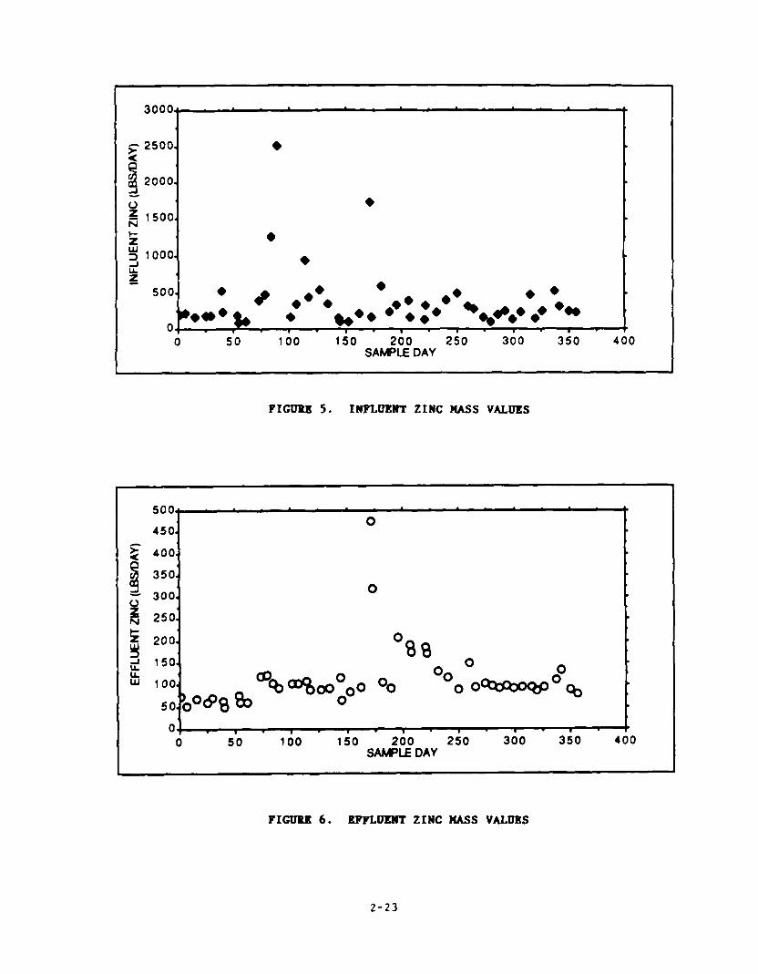
I I I 1 I 0 50 100 150 200 250 300 350
SAMPLE DAY 400
PItxrm 5. INFLUEHT ZINCWS VALUES
400.
350.
300.
250.
200.
150,
0
OS8 o OO
0
OO 0 O-QQPOB
0 0 50 100 150 200 250 300 350 400
SAWLE DAY
PIGII'IU 6. KFFLUlS.NT ZINC MSS VALWS
2-23

TABLE 4. ZINC MASS VALUES (LIE/DAY) AND DAILY REMOVALS

system was experiencing some operational difficulties or interference at the
time. Inquiries should be made to determine whether there are valid reasons
for dropping these data for purposes of calculating removals.
Influent zinc levels versus effluent zinc levels are plotted in Figure 7.
The removal efficiency on December 19, 1987, (72.23 percent with an associated
influent value of 1,750 lbs/day) contrasts sharply with the removal efficiency
on September 27, 1987 (95.25 percent with an associated influent value of
2,500 lbs/day). Thus, the data show that the POTW was capable of treating
influent zinc considerably above 1,750 lbs/day.
Figure 8 is a plot of the daily removals over time. The three negative
removals are quite apparent from the plot. It is asswned for this example
that justification to discard any of these data was not possible. Negative
daily removals should not automatically result in data elimination; such
values may be visible evidence of treatment system variability. Based on the
51 daily influent, effluent, and removal values, the summary removals were
calculated: the average daily removal was 53.4 percent and the mean removal
was 69.5 percent. Note that the two removal averages are considerably
different. (Had the influent and effluent data for the negative removals been
discarded, the removal averages would still have been considerably different;
average daily removal would have been 59.6 percent, and the mean removal would
have been 72.4 percent.)
The decile approach can now be used to evaluate these removal averages
with respect to the nine decile estimates. Table 5 presents the ordered daily
removals for use with the decile estimation worksheet.
Table 6 presents the results of using the worksheet. Since the number of
influent and effluent zinc data pairs is 51, the entries for Column #l are,
again, multiples of 5.2 (see the first footnote at the bottom of the
worksheet) Likewise, the entries for Column #2 are the whole numbers of
Column fl. The ordered removal entries for Columns #3 and 84 are taken from
2-25

5004 L
450. d
.
$ 400.
0 0 a
O+ . . . 1 t 0 500 1000 1500 2000 2500 3000
INFLUENT ZINC (LBSDAY)
?IGms 7. INIWJKNT ZINC VI. KIVLCKNT ZINC
2-26

120
100
60
d
P
:: c
20 0 % -20
-40
-60
150 200 SAMPLE DAY
?ICURX 8. DAILY PERCENT RlQ!OVALS FOR ZINC
2-27

TABLE 5. ZINC HASS VALUES (LBS/DAY) AND ORDERED RICHOVALS
2-28

TABIJi 6. DECILE ESTI)(ATION WiU3lIXT FOR ZINC DATA
a.65 1
AI0 I
m.n 1
fnTRlEE 1
-n +r calm defined IS ultlplts of (ll+l)/lO. rlwre a = the ntder of data pairs used.[i.c. (Sl~~/llkS.2). (2x5.2=10.4) etc.] -uses the list of ordered rmuv~lr.
2-29

Table 5. Column /}5 is obtained by subtracting Column 83 from Column #4.
Column #6 is the decimal part of the entries in Column i/l. Column //7 is
obtained by multiplying Columns H5 and 16. The estimated deciles, Column I/S,
are obtained by adding the entries of Column 13 to those of Column /7. The
nine estimated deciles for the zinc data are:
l 1st decile - 18.0 percent
l 2nd decile - 36.3 percent
l 3rd decile - 46.2 percent
l 4th decile - 55.7 percent
l 5th decile - 60.0 percent
l 6th decile - 65.0 percent
l 7th decile - 71.6 percent
l 8th decile - 78.4 percent
l 9th decile - 83.0 percent.
The decile estimates then can be used to estimate how often the POlW’s daily
removals of zinc exceed the average daily removal of 53.4 percent and the mean
removal of 69.5 percent. The former lies between the third and fourth decile,
and therefore is exceeded between 60 and 70 percent of the time. The latter
lies between the sixth and seventh decile, and therefore is exceeded between
30 and 40 percent of the time.
2.4.2 NICKEL SAMPLING DATA
The last example involves working initially with a data set of 51 daily
fnfluent and effluent nickel mass values. Table 7 presents reported influent
and effluent values and, when possible, their daily removals. The table shows
that a number of the daily removals cannot be determined because of reported
zero influent levels. J’hese reoorted zero levels more than likelv indicate
In this section,
the reported zero levels are treated as measurements having the value of zero.
For discussion of this practice and alternate approaches, refer to Section
2.6.
Figure 9 is a plot of the 51 influent nickel mass values over time. The
large number of zero influent values is apparent along the horizontal axis
(sample day) ; the zero values are spread out over the sampling period. An
2-30

1404 b
120. l . 1
100.
80. 80. l + l + l l 4 4
60. 60. l l
l l l l 4 4 l l 4 4
40. 40. l l l l 4 4 l :* l l :* l l l
l l l a l * l a l * 20. 20.
4 4 o+w.* o+w.* #A #A .-*.* .-*.* v--a v--a . . 9 9
0 0 50 50 100 100 150 200 250 300 350 150 200 250 300 350 400 400 SAMPLE DAY SAMPLE DAY
?ItxJu 9. IllhunT IIICXL MASS VALmsS
801 t
70 0 0
60
0 0
00 0 0 0 0
0 O 0
O 0
IImRn 10. JImLmmI IIcKxL HAM VALUES
2-31

TABLE 7. NI(SICEL IGUS vALDl!S (LBS/DAY) AND DAILY pwOvALS

isolated influent nickel value around 120 lbs/day also exists. Table 7 shows
that the daily removal for that influent value is 100 percent because the
corresponding effluent value is zero.
Figure 10 plots the 51 daily eff-luent nickel mass values over time. The
effluent nickel values also show a number of zeroes, many of which will not be
used because their corresponding influent value was also zero.
Figure 11 plots influent nickel mass values versus the effluent nickel
mass values. The horizontal axis shows that there are a number of influent
nickel values above 0 (ranging from about 25 to 120 lbs/day) that have
effluent levels of 0 (that is, 100 percent removal). On the vertical axis,
four influent and effluent sample pairs for which the influent was zero and
the effluent mass level was greater than zero exist. Since daily removals
cannot be calculated from influent values of zero, any influent or effluent
data pair (regardless of effluent level) having an influent value of zero will
be excluded.
Figure 12 plots the daily removal values over time. The figure shows
that the POTU displays some treatment variation. The positive daily removals
vary from about 10 percent to 100 percent. The figure also shows 4 negative
removals ; 3 of the 4 negative removals are similar in magnitude, about -15
percent. The other negative removal corresponds to an influent nickel mass of
32.55 lbs/day and an effluent mass of 65.09 lbs/day on March 16, 1988. These
sample pairs should be investigated to determine whether the data should be
retained. Except for the influent data values of zero, it is assumed that
justification for removing the data from the process of calculating average or
decile removals was not possible.
Table 8 presents the 24 influent and effluent nickel values that were
used to determine individual daily removals (i.e., 27 influent and effluent
sample pairs were excluded because the influent nickel level was 0). The 24
influent and effluent values are ordered on the daily removal values. The
average daily removal based on the 24 daily removals is 61.6 percent; the mean
removal value determined from the influent effluent data is 63.0 percent. (If
2-33

70.1 II
60.
I
= )I II
I 1
20.
1 0.
40 INFLUE:: NICKEL $S/DAY)
100 120 140
- 5 0.
-7 5.
-100. l
-1254 I r I I a ? 0 50 100 150 200 250 300 350
SAMPLE DAY
PIcnm 12. DAILY PERCRMT RlWOVALS FOR IIICKKL
2-34

TABLE 8. ilIclcEL MASS VALUES (LBS/DAY) Arm ORDEBLD imlovALs
2-35

the 4 negative removals had been excluded from the data set, then the average
daily removal, based on the remaining 20 influent and effluent nickel values,
would have been 81.4 percent and the mean removal would have been 76.5
percent. )
The 24 ordered daily removals of Table 8 are used in the decile
estimation worksheet presented in Table 9. (The entries for Column {/l are
multiples of 2.5. Column #2 uses the whole numbers of Column 111. Columns #3
and //4 use the ordered removals from Table 8. Entries for Column {I5 are
obtained by subtracting Column //3 from Column #4. Column #6 is the decimal
part of the entries in Column #l. Column #7 is produced by multiplying the
entries of Columns #5 and #6. Finally, the estimated deciles are produced by
adding the entries of Columns 113 and 117.) The nine estimated deciles for the
nickel data are:
l 1st decile - -
l 2nd decile -
l 3rd decile -
l 4th decile -
4 5th decile -
l 6th decile -
l 7th decile -
l 8th decile -
l 9th decile -
17.0 percent
13.8 percent
47.7 percent
57.5 percent
100 percent
100 percent
100 percent
100 percent
100 percent.
The average daily removal of 61.6 percent and the mean removal of 63.0 percent
both lie between the fourth and fifth deciles. That is, based on the 24 daily
removals, these average removal values are exceeded between 50 percent and 60
percent of the time.
2.5 OTHER DATA PROBLEMS
Some of the difficulties that can be encountered when examining sampling
data used for removal efficiency calculations (e.g., extreme values for
influent, effluent, or daily removal; or negative removals) were previously
illustrated. In this section, two other data characteristics are discussed
that may require special consideration in determining removal efficiency.
2-36

TABLE 9. DECILE ESTIMTION WORKSHEET FOR NICKEL DATA
I nwwhl 1 m.rr 1
FalQIute 1 EWRY I LIST WE I TIE I nlun I #CIW
I CQ. n 1 rm.n 1 II I WNF 1 Wflll I ml. n
I wl.n 1 a. n 1 I tr1n I WNIES I I m I I I m.c6 1 WTIMTW 1 I WNT I DECIKS I
I 7th I /w I 17 I . . . . . . . .._ I I . . . ..-.-......- *..----.----.----
I 9th
I
Clukrs in colrrn &fined as mltiplcr of (11+1)/10. here II r the nuder of data pairs used.[i.e. (51+1/10-5.2). (2x5.2=10.4) etc.)
-uses the list of orb-d NkmrJrals.
2-37

2.5.1 REMARKED DATA
Sometimes influent and affluent concentration values are mt rtou
m. For example, some sample values may be reported as Not
Detected (ND), or Below Detection Limit (BDL), or less than some specified
value. These types of values can occur for either influent or effluent
samples. For example, assume that the following influent effluent sample
values were obtained:
SAMPLE DAY
INFLUENT EFFLUENT DAILY LEVEL LEVEL REMOVAL
1) -clludL EFFICIENCIO
1 100 40 60 2 200 ND 7 3 240 60 80
The remarked data values result from limftatlons in the analytical
methodology used for the chemical analysis. How should such data be dealt
vfth? A common approach applied to remarked data is to substitute a specific
quantity for it. For example, suppose that some effluent samples were
reported as ND and the analytical method that was used has a detection limit
of 10 mg/l. A substitute value of 10 rig/l for each ND might be provided and
then any calculations using that data value performed. Variations on this
approach are to substitute half the detection limit (e.g, 10 x .5 - 5 mg/l),
or even 0 for the not detected value. For the above example, substituting 10
mg/l, 5 mg/l, and 0 q g/l for the ND value uould result in comparable daily
removals of 95 percent, 97.5 percent, and 100 percent, respectively. However,
if the influent concentration value associated with the effluent concentration
value of ND were smaller, say 40 rig/l (instead of the 200 mg/l), then
substituting 10 mg/l, 5 rig/l,, and 0 mg/l for the ND would result in daily
removals of 75 percsnt, 87.5 percent, and 100 percent, respectively. These
latter removals demonstrate that the daily removals can be affected by the
choice of value that is substituted. When replacing remarked data with
quantitative values, it is important to determine whether the various
substitute values produce substantially different mean or decile removals.
The most obvious way to determine this is to perform the necessary
calculations using the different substituted values and then to compare the
final results.
2-38

2.5.2 SEASONALI’N
Seasonal treatment performance variability can be monitored using the
time plots of influent, effluent, and daily removal values. Variations in the
removal efficiencies that can be traced to seasonal patterns may suggest that
average or decile removal efficiencies for specific time periods be determined
or that treatment performance be improved for specific time periods.
2.6 NONCONSERVATIVE POLLUTANTS
In the 1987 local limits guidance, a distinction is drawn between
conservative pollutants, which are not degraded or volatilized within the unit
processes of a treatment plant and nonconservative pollutants, which are, to
some degree, biologically/chemically transformed and/or volatilized by
wastewater aeration/turbulence within the POTW’s unit processes. Conservative
pollutants exit the POTW solely through the POTW’s effluent and sludge
streams, whereas nonconservative pollutants are also destroyed by chemical
reaction (e.g., microbially mediated oxidation) and/or undergo a phase
transformation from wastewater to ambient air.
Removal efficiencies considered to this point have been solely for
conservative pollutants, such as metals. Conservative pollutant removal
efficiencies are determined by pollutant concentrations in the POTW influent
and effluent streams. The presumption applied to conservative pollu
tants, that removal pollutants are exclusively transferred to the POlW’s
sludge screams, cannot be extended to nonconservative pollutants. Losses
through degradation and volatilization do not contribute to pollutant loadings
in sludge. As a consequence, nonconservative pollutant removal efficiencies
cannot be used in deriving allowable headworks loadings from criteria/
standards applicable to the POTW’s sludge streams* (e.g., digester inhibition
data, sludge disposal criteria/standards). An alternative procedure should be
used.
* Removal efficiencies for nonconservative pollutants m be used to calculate allowable headworks loadings based on pass critu (e.g., biological process inhibition data, NPDES permit limits, and water quality standards). The removal efficiency guidance provided in this document can be directly applied to nonconservative pollutant removal efficiencies obtained for this purpose.
2-39

The 1987 local limits guidance provides the following equation for
deriving nonconservative pollutant allowable headworks loadings from sludge-
based criteria/standards:
C CIIIT L IY - L**r x
C SLOG
or C CR11
L IN - GLDchkF
where :
L IN - Allowable headworks loading, lbs/day
L IW - POTU influent loading, lbs/day
C CR11 - Sludge criterion/standard, q g/l
C SLOG - Pollutant level in sludge, q g/l.
In the above expression, the factor CILoJLIMc is a partitioning factor relating
the pollutant level in the POTU sludge (C,,, ) to the headworks loading of the
pollutant (L,,) . The partitioning factor enables calculation of an allowable
headworks loading (L,,) from a sludge criterion/standard (C,,.,) for a
nonconservative pollutant. To determine the partitioning factor for a
particular pollutant, the POTW’s influent and sludge must be routinely
monitored for that pollutant.
It is important to recognize that the factor C,dL,,, expresses
nonconservative pollutant removals to sludge. Nonconservative pollutant
removals to sludge are highly variable, and are dependent on such factors as
wastewater temperature, ambient air temperature, biodegradation rates (which
are temperature dependent), aeration rates, and POTU fnfluent flow. Since
nonconseNative pollutant removals to sludge are highly variable, the
resulting variability in nonconservative pollutant sludge partitioning factors
should be addressed as part of the local limits development process.
2-40

The procedures and recommendations provided in this manual for addressing
removal efficiency variability for conservative pollutants (e.g., the
calculation of mean removals and the decile approach) can be extended without
modification to addressing variability in nonconservative pollutant sludge
partitioning factors. In calculating sludge quality headworks Loadings (see
Section 2.4), the sludge partitioning factor should be used in place of the
removal efficiency for nonconservative pollutants. This sludge partitioning
factor can be entered into .
2.7 SUMMARY REMARKS
In this document the following three methods for removaL efficiency
estimation have been defined and illustrated:
. Average daily removal efficiency
4 Mean removal efficiency
. Dee ile approach.
The first two methods provide single point estimates of POTW removal
efficiency. The average daily removal is simply the average over available
daily removal efficiencies derived from paired influent and effluent
wastewater samples. The mean removal efficiency is the sum of effluent
loadings divided by the sum of the influent Loadings. The mean removal
efficiency weights influent/effluent pairs with a higher flow more than
influent/effluent pairs with a lower flow.
In general, these two methods of estimating removal efficiencies yield
different results. Of the two, the mean removal efficiency is preferred
because it is less sensitive to extreme daily removal efficiencies.
The decile approach is more comprehensive than the first tvo methods
because it yields an estimate of the entire frequency distribution of daily
removal efficiencies, Using the decile approach permits the explicit
incorporation of the variability of daily removal efficiencies into the local
limits development process. Actual removal efficiencies derived from actual
paired influent and effluent wastewater sampling data demonstrate that daily
2-41

removal efficiencies are not constant over time. Daily removal efficiencies
demonstrate considerable variability; a single value approach to estimation of
removal efficiency can only provide an individual measure of the actual
process.
Computationally, the decide approach is more data intensive than both of
the other two methods. For example, the decile approach requires a minimum of
nine daily removal efficiencies; whereas the other two methods can be applied
to less data. From the standpoint of statistical precision (difference
between the estimated removal efficiency and the unknown true value), the mean
removal efficiency is the most precise. Decile approach estimates can be less
precise than either of the mean value sstinates. These statements regarding
statistical precision apply to the respective estimates derived from the same
number of daily removal efficiencies.
In cases for which removal efficiencies are consistently large (e.g.,
greater than 80 percent) or are consistently small (e.g., less than 20
percent), the acceptable statistical precision can be obtained with a small
number of daily removal efficiency values. Even in these instances, no less
than five daily removal efficiency values should be applied. The data set
size should, however, be increased to a larger number whenever the daily
removal efficiencies exhibit more variation. In most cases, more than the
minimum number of daily values should be used in the estimation process.
2-42

APPENDIX A
ADDITIONAL RESIDENTIAL/COMMERCIAL DATA

A.1 RESIDENTIAL/COMMERCIAL TRUNK LINE MONITORING DATA
I 11 b
n n OOWO DOW 0.27J 0.002 n n OObbO OOY 079 0077 n Jo 0.W 0001 0.276 0014 n n 0.m 0001 0.076 0.017s n 1 0.0160 OQol 0.21a om7 1) n O.ooO OWl 0.124 O.QoI n Jo 0.0020 0001 0.01 O.Wl
,
2 2 0.1= 0 120 0 144 0 1Y 2 2 OCOOQ 0.S 0 11 0.1 2 2 OOWO 001 0 07 000 1 2 O.OOW co.006 0011 0.001
2 lb0
. b 4 4 . J J 2 3 2 2 J 2
b b b b J b b . . . 3 J b J J 2 J 2
O.TOOO 00011 0007 0 0474 OWJb 0 0130 OOOQ OWW 000&l 00062 00072 OOOW 0 0010 Ooo(y OOOW OW
O.OOW3 OWOOI OoooOl
01 006 OW
00076 00016 coo02 OOWb
OOWW 0m 00002
OWOOl 0002 0001
000001 OOOQZI 0-1 OOWO2
OOOOOOb OOOWI
07 0 1676
001 0.1 0.1
Oojl 0.W
Oop 0 01 0 01
OOOI 0002 0001
<owl O.ooo1
co- OOQXD Omool OoWOl
07 oon
oom 0.01 001
a002 0.01
O.oQ1 OWbJ 00062 0.0024 0002 0001
do001 O.WWO Omool
0.- O.wml OOoool
A-1

A.1 RESlDENTlAL/COMMERCIAL TRUNK LINE MONITORING DATA
u U O.OIQ Oop 0.2 0.0. u 0 0.W 001 0.01 0.W 7 U 0.U a.wb 0.12 0.m
u u O.Om 0.01 0.m a.- 14 U 0.0001 a.w7 l .a aa
L
N
76 u a bl
76 U a W
0.3144 0. Ia la Oa, 0. 1w 0.0, 0 a7 0 0 Ootlb OOOU 00, OOlU 0.W O.ooOM O.Ol@ OOQZW
b
10 10 OIOO 03 I4 OI 10 10 OIIOO 0.1 00 01 10 IO 0.1600 01 0.4 01 10 IO aBow 0.1 0.1 0.1 1 1 0.W 0.1 0.1 0.1
b
12 I2 0. 1oI I 7 0.1017
12 12 0.07n 4 8 O.Ol#a 10 10 0 @loa B l 0.0117 2 2 0.016 b b 00014 2 2 0.003
0.01 0 01 001
0007 0007 OOOI owl 0001
OoQ)s
0.27 0 a7
0 11a 0.011 0.01
O.op O.OW
O.op O-o005
01n 0.06
OOU 0.0106 OOlY OOO
O.Wlb 0.013 O.ooo1
A-2

A.1 RESIDENTIAUCOMMERCIAL TRUNK LINE MONITORING DATA
Ml b
5, 5, m a 21 21
0. 1w O.W7# O.ooL 0.W 0.W 0.m
0046 0011
awl do01 Q.001 Q.001
0.,7# 0.182 O.wI 0.072 O.Nb 0.001 r.on O.NOb O.Dy O.oDp 0.007 0.002
b 0.01
140 140 140 1yI 140 140
001 0.2laa 0. la2 0 0610 0.0117 o.ooy
O.oI a1
a006 co.06
0.06 do.006
140 01
130 12
7 00
0.76 0 61 0 01 0 12 0 14 ON
02 0.18 0 12
-306 coa
ro.006
007lo 0010) 0.W OOUO 0.010 0-1 ow21 O.ooo1
Oo(8 4006
a02 002
OOOZ COW1 OWO2 OQ101
008 42
Oo(l 0 07
a.w co.01
<o.oN OWW
0.W O.QT QOL 003
a.006 owl2 00021
00002
1.2 80
1.m lb 07OW ON OW OU
0.4.W 022 0m 01
0.1100 001 00171 co oml
00176 OQY 0 0166 0 014
24 1.u 0.m 07 0.N 07 0.74 0.0
OS 02 0. la 0 11
OOU 002ll 0m OOl?b 0017 00166
A-3

A. 1 RESlDENTlAUCOMMERClAt TRUNK LINE MONITORING DATA
-~ - _--___ _-----__- - ____ - _____ --- __---_.------ ---
2 2 0 0076 owr 0006 0 Qo7b 1 2 0.00 a006 0007 O.W. 2 2 OONO 0.001 o.w7 0.004 1 2 OQOIO OWO cow6 0.004 2 2 O.ooY 0.002 O.Wb O.OWb
l-23 u
2 2 2 2 2 2 1 1 2 1
2 2 2 2 2 2 1 1 2 1
am OIIW OOOO OayO OO#W 0.W O.OW!O a.090 0.M 0-W
2r4 m.2 a.0 O.o( 0.78 041 OW 0.42 04 0.Y 027 0.1y 006 0.11 O.Q( 0.W 0.0 O.oW
O.OU mu 0.W 0.04 0.01 0.N 0.03 0.4)1 OOWb
O.oa, o.aam O.OU
a (0
OWN 0.016 l.IY 0.10 0.1* 0.001 204 0.076 0.M 0.01 0.Y 0.07 O.WlO O.OW 1.0 B.oL 0.M co.Wl4 1.2 0.a 0 OlW Q.007 low 0.007 0.0127 coo01 0 11 DOOI OW OWN OOW OW3 O.WlT Ooool 003 OOOW
187 164 IY 181 In 214
2? 13 23 I7 .
27 u 111, ? 11. n a 007n 003 0 lb 007 26 oom COO1 021 004 2s 00x)? CUooQt 00 002 27 00301 0011 0066 0 0276 2a oomo 002% 0m 0028 27 00163 OOW Om? 0006 26 0 01m COO01 006 cowb
1 11
A-4

A. 1 RESIDENTIAUCOMMERCIAL TRUNK LINE MONITORING DATA
LxmNmD TOIM MIyanc MlJueEROF NJuaERoF AVERUY YNNlm YAXMLN UEDbM -8TlC FLOW cowlmrw MEClKMZ3 ONEFWATy*(B RXLUTAM POLLUlbNl pocLulAm POLLUTW
ClN STATE fEavm wm F) LEutL LML LML LML
(uan) (uonl NW (ucu)
--- ----- --__--- ---- --__-I__ -- _-___ -__ ___- ______ _
1 a OOlP 0013 OOlJ 0013 17 2a OOIW <o 001 001) OON
2 n OWU 0006 0.008 0.W.b . 26 OWW cuow 001 a.002 2 26 OOOY .s.ow 0.01 +o.om
on 10
3 ¶ loo@7 00 1Y 12
1 1 0.2100 0 210 0.21# 0.216
s 3 O.ocQ 0.036 001 0.W
J 3 OQ3u 0 014 0017 0.W
1 3 0 0516 0.0164 4001 a.04 I 3 owm Q.wb OW cow
1 J mm8 0.003. a.w <o.w
~ -___- ____-- - - - - - - - -_ I_ ~-- I__--
A-5

A.2 COMMERCIAL SOURCE WASTEWATER MONITORING DATA
1OlM WROF WUYWAOC WUYYROF AWXM3E ylww MAXYUU UEmM
ITAlE RO**I SJUWXFLOW ma CMZIECTW aPWN*Im FWLLU~NCV LEVEL FQLLUlAHT LML po(LUlU4l LML KXLUl*JIT LEWiL
WV (uon) (uanl wow (UMJ -______-_ -____ ___ - .______ - -_-_ ___-__.- -.-_-- ------ -------------- --------------- .---------------- -------------- --------
OWN
0 0714
oob.1
OWbb
<o 03
COO6
co 001
soool
0 17
OP
01
002
?A a
OWW
OWW
002W
OOloe
0 07
awl
002
cow7
00
0 18
002
002
001
00)
002
001
PA 5 17mw 3
0 64la7 01 07 -TE
17 VA 5
10
u
0
1u
22
11
2m
a
10 3OOlWO
w 242m
61 OCUI
1Y 0 L)?.
62 0 1w
67 0-
.w Owol
61 OrmS
20
006
coo2
co.01
coo6
0012
a01
-00s
a07 40.
a. 0 lb
IO l 0 1.
a. 0.
1U 406
OY <ow
IQ cow
OY 0.001
KY 4
W e2
67 W
Q 02
3 J
W P
Y W
W P
u W
u P
40 82
Y a
46 m
u W
22404
I mr
OloI
024.J
0 21n
0 law
OOUO
OObM
00304
00117
00072
OWW
owl?
022
OW
0 07I
0 la
00%
owl
000.
co 03
OWl
0 0027
0003
coo02
co ow2
361 101
I76 OCM
lb 0 on
011 020.
10 0.141
224 00)
2b 0 01a
oa 004
0a 001
ow 001
006 OW
0 01. OW
0022 OOOOO
A-6

A.2 COMMERCIAL SOURCE WASTEWATER MONITORING DATA
TOTAL HlJuHRW -0c NUMBER OF AbtFwx ww WlmJu maw4
WATE IIEaca -FLOW WUIUSS DzILcTm WFWAlm FOLLUTAM LEEl F’CXLUTAW LML PocLuTAMl LEN3 WUTMfl LEXL
(opq WI (eon) ww (UCYI) --- - _-_-_- __-- _-__ ______ -__-- -_- ______._ - -------- - _.-_ ---__-_ _--_- _-__ -___ _-____
12
Y
10
1,
a
1,
I1
10
20
a
26
7
I
b
2
3
uI.ban
m.aa2
32mo
llw8
O.-T
O.bn?
O.plT
OllDI
OOTab
0.0101
OOU
OW
oot.4
0010~
00100
00016
331
ZQ
1Y
0.62
0.0
00)
0001
002
0.002
0.001
0001
0006
OWI
0003
0004
owl
baa 40?
1W a4
a.6 a.3
40 10
2? 0 II
4.6 0 1s
1.3 0 ib
OQ 0.01
OLOZ 00s)
OW 001
0602 0 01
01 0a
001 002
OW Orn?
OW 0 05
OOOZ 0m
A-7

A.2 COMMERCIAL SOURCE WASTEWATER MONITORING DATA
na
163
J.al
1.?4
13
123
1 ia
0 11a
oQ27
Y
483
¶.Jl
1 ?4
13
I23
1 1J
0 11a
0.027
12
442
44
*u
4a
n
146
005
006
002
OOC
003
OWb
ra
Jx)
622
OW
2.w
a4
0076
0011
Py)
J2a
OIID
.
.
1
IO 0
I@
0 *I
al
-3
I1 I
421
n 76
3.4?
b
<o 2
01
006
002
001
001
001
0 014
OWOI
tra
??O
346
126
1.
01
062
OOOI
ow12
703
10 11
la84
O&4
-32
004
001
0022
cooQxI1
2
1
.
0m
044
OOWb 2
A-8

FoRTclooOE
A.2 COMMERCIAL SOURCE WASTEWATER MONITORING DATA
m I no0 a
20 20 1~.1180 008 110 a.2
10 a b2.m a02 (12 3
P 20 21 mm 0.12 II, 0.Y
217.1&M
ballu
20.2774
0.2Ub
O.lY7
0.1tm
0.001
0.01-a
O.oQ
22oa
1.m
2121a
O.oU
o.ola
o.ola
O.Oll3
0.01.
O.OODI
0al.M
WLW
87.ama
0-m
0.1)tO
O.dZN
O.oU
O.osl
O.all
3.ba
so.au
rU.1
0-1
0.w
l .W O.oY
0.M 0.M
--
A-9

A.2 COMMERCIAL SOURCE WASTEWATER MONITORING DATA
TOTAL IaJuuiRoF MuuwFloF NUWEROF Akmmx MAXYUY -
OTATE WW3N -FLOW m OETECTM OOWIWAT- POLLU7AwTLML POLLUlMLfM3 POUUTAMLfVEL PQLIK LEML
(oral W@U W) (UOA) WW _I____ ------- -~---- --__- - ------ ---- -___---- _-_-_-_-_ ____
m 1 am
PA a
a1
2b
2a
I7
14
a
21
51
P
27
a
2b
12
n
0 ml4
0 lrn?
0 14a
0.0013
OOb2b
0.0170
O.Olb7
1a.n
0.2Iao
0.W
0.W
0 la
OOQ2
004
002
a02
CO.001
a.002
Y
004
0.070
a.ob
a
08b
03
02b
0%
a06
0.07
110 ab
0.2. 0.211
0. I2 O.Obb
0.0 O.oY
0.0
0.078b
0 1P
o.on
a.00
0.01
a.01
-- - ___-- ----
A- 10

A.2 COMMERCIAL SOURCE WASTEWATER MONfTORlNG DATA
VA
u
a
moo
27
.
a
Y
Y
b2
Y
P
u
b
b
28
1
b
11
20
18
zo
a
Y
22
0
I
2
1I
1
b
aI IlIl4.ma2
4 7.w
a au
Y 2llO
b7 OAIO
Y 0.m
Y O.Itp
bl O.lZI
0 0.m
b
II
0
I
a,
a
10
W
Y
a
W
17
P
I4
2b
lb
22
1oy.moo
l41o.m
YY
7.a
loo,
1.m
0. Ion
0.W
0 1lW
0. I la
O.lOSJ
O.ooO
O.oQ
O.Mlb
ootn
0.01a1
0.0124
00
4.8
0.0
001
a.-
am
a.0
a.02
a.ab
YI.oQo
aana
0.000
000
O.DoL
0. IW
o.eto
0.007
0001
0.004
0006
OQIO
O.oQ)
O.oo(
0.W
0.001
OOOI
1MoQ
I%.\
m.n
a
a4
1.Y
I.o(
0.a
0.427
11700.004
474o.noo
2wooo
Y.zw
l ooo
am
0.W
1.100
2.100
0.470
010
OIIO
OIIO
0 la0
0.2S
0 10
0.W
a.40
au
2.OT
0.U
0.12
l .U
0.1
a.46
0.00
lUhoo0
121aLoo
0.010
2.ooo
8.110
0.Y
o.on
O.QD
OOOI
aom
O.oI
0.W
o.oIo
O.op
a.010
0.01
0.010
-- -- - ---- ------- -
A-11

A.2 COMMERCIAL SOURCE WASTEWATER MONITORING DATA
TOTAL 6aJMeEROF WJYYROF NlNaEFloF A- MAxmlN MEW
8TATE Roo1 OOUFCEFLOW DUNbXI rNm%Tm -ATII(Q PCUUTM LEXL POUUT~ LEXL POUUTMT W POUUTAMT IENL
WV NM) -1 W=) Cwu) - -_ __I_ ---_- -_---_-- _I-_--_- _____---_ ______ ____ -_
m 1
MLEN-lM
zwc 6 6 0 1740 0 01 026 017
-A 6 6 OW 0.06 0 12 000
LEAD 2 6 00270 cocQ6 0.m a026
-0l 6 6 OOWU 002 003 0.02
NKXEL 3 6 OOOQO coca7 0 01 001
COIAlT 5 6 OOM4 Co415 0.01 -so43
1X40
Imoo
OWOO
OWW
DO420
00200
0 Old0
13
12
0.Y
0.3?
0042
0.02
0.011
13
12
OW
0 3?
ooI2
002
0 010
13
12
OUI
037
OM2
002
0 010
PA a
TDB
coo
PHOOPHATE
ubcw
UXI
2
1
I 1 dzdoooo e6 m6 a6
b2 6? 316.6647 1 na 1W
cm 31 2&7lso 0.1 w7 1
1 1 0 6100 O.bl 061 0.61
8 b 0 1170 0m OU OOb26
I 2 00660 a.o( OOb 0.W
1 2 0m DOW ,301 0.W
---- ---- ------ ---- _----- - ------- ---- _-_- ---- --_---- ---- --------- - __------ - -----_- --_-- ------~
A- 2

A.2 COMMERCIAL SOURCE WASTEWATER MONITORING DATA
TOTAL IaMeEROF l8lmBLR OF IluMaiRoF A- wyw MAxYlJM w3IwI
BTATE fW3lOU -FLOW &W@UXI rsmxxlaa OOlJEfWATm RJLLUTMT LEWL PouuTm LEVEL muuTA)(r LEwil mLLuTMf7LEmL
(CQq (uQI1) -1 (UOA) (uan) ___- ~ __ --__ ------ -- ___-_--- ---_-- - ---- -_--- - ----- --_--- -------- ___-___--
1 1
6
b
1 a7.0
0 4100
0m
O.twD
0 2lW
0.1m
0006.
0.W
0.W
0.M
O.OIY
O.OIW
o.oia 0.0010
0.e
0.n
OW
OS
0.2
00.3
O.DI
00.2
O.op
aola
002
0.01. o.ot2
O.OS
0011
0011
22
011
036
0.U
0.Q
OP
0.N
0.061
oow
O.o?
0.W
0.012
0.05)
O.OIb
0.011
I.5
0.Y
0.S
03p
OObO
0 I2
0.M
0.W
o.Qaa
0.02
O.OO(
0.012
O.OOb
OW
OOOI
b
b
b
b
b
b
1
b
1
b
b
b
sub 2
W
*
16
n
ia
11
lb
OlDI
0 0182
0.*7
oa27
0 1Qy
OW72
ooaoo
3207 OISY
42 002S
2.0.7 023
lyI? 0 11
02b. 0 01)
021 COOL
0 1. DOlW
UFMO 2
6
*
e
0
b
b
b
b
b
b
b
b
131000
2m
I tom
0 rm
OOU
OOU2
0O.b.
002b4
0m
OW
owe2
OOOU
4.
02
Ob.
0 1.
COO01
corn1
COW1
COO01
<oool
co 001
COO01
<o WI
18 4 172
168 03
2.76 on
1* 02
00 ~001
0 1.4 -zoo01
0 I# a001
001. a002
00 COOI
aw2b a001
ao2b a001
a026 cow1
1
1
2
A-13

A.2 COMMERCIAL SOURCE WASTEWATEA MONITORING DATA
20
MO
*p
4a
147
lob
140
111
b
Y
2M
Ml
Ml
4n
na
m
277
m
Ia
II
ln4m20
2.a
I.aza
0.01.
0.M
o.a410
0.011
o.opn
0.014.
a.014
?I
4.w
0.03
-no2
0.01
a.01
a04
Qmb
a.001
d.owz
zmm
i-a4
au
14 b
nb
l .bl
OY
0 bib
001
O.ooO
lmo
108
0.4
O!dO
OW
000
004
OOlb
001
O.amb?
4
1
I
II
I
n
Y
14
z!b
21
Y
1 74.mm
1 aL1ooo
a lb.&?10
1 lo.oooo
n 2a
Y l.alz
ab oe1s
a0 OIDI
71 014n
1 o.obn
I4
12
Co.01
IO
OZU
0 lb
CD1
coob
a.04
a.01
74
n
Mb
14
bab
700
bm
on
040
0.a
?4
a&b
l Y
la
l?n
001
0.4b
0 10
0.12
OQU
KV 0
37
a?
a4
a?
a?
a0
aa
P
n
lb
a
n
a7
a?
a?
3?
31
17
a?
J?
a?
ar
ar
ar
l .?mo
l.J.1#
0.M
0.m
OMM
O.zY
0 101
OMOb
0.09
001a
0.0100
O.On
27.1 l .42
442 OI
1 74 OU
Ib O.b?b
1 1 048
b.1. 0 162
2w 0071
011 0.021
CU.1 001
001 a.01
0.05 O.oO?
0.017 0 Ootb
own
0 low
OOOO
o-7
OOm
0 Ol?b
OU
0 I1
003
coo
COO3
-301
no
oa
0 I4b
DO1
coob
0027
Ob
0 ta
OQOL
045
003
coo1
A-14

A.2 COMMERCIAL SOURCE WASTEWATER MONITORING DATA
L b 121oooo 14
on b
b
a4# %b
2M %4
2s au
3 %b
2n %l
I#2 Yl
117 117
b2 aM
1n aab
l.UB4
0.41n
oztn
0. la0
O.lYI
0.019
0.010)
O.Qp
O.OWO
01
0.1
0.01
0.1
0.01
0.01
0.001
0.01
O.WOl
Ml 0.7
lb 7 co.2
2.44 0.00
or 0.2
12.b 0.0)
b.Ya *o.aY
OAO? 0.0%
0.P co.02
0.004. am
10 10 7.a
10 10 21am
10 10 1109
10 10 0.7S42
lb 10 O.l4?4
13 10 0.1r
7 10 O.M%
1
0.2
0.1
0.1
CO.1
a.1
a.01
20.0 &b
7.3 1.7
4.2 03
2.2 0.7
0.b 0.1
03 0.1
0.1 a.01
77 77
II b4
w 67
n 81
a7 70
bo bl
2.1071 0.14 b.4
1.W 0.n a
0.n O.Oa bb
O.Y7b o.on 0.72
0. lua CO1 0.00
0.W O.Olb 0.23
2
0.a
0.78
02
co.lab
0.017
4aooo
a
2
a
1
a
1
a
a
a
a
7
bo
22
4b
4 1lQ.m
a l(o.ooO
4 lLo.oQD
4 l .rur
4 l .w
4 a.wI
a0 UOZl
4 2.12m
w l.WM
a 1 on7
0 0 MT1
m 0 P?lb
P 0 llra
u 0.110
<lrn
<lW
<lW
(1.47
(12
c0.a
0.U
<i a
CO.1
OY
a01
OW
0 01
OOlb
l&O
lb0
W.b?
12.#7
1l.b
la
a10
b.47
20
a4
I Ia
043
00
lb0
1Lo
ILO
(I.47
bO28
4.a
2.Y
1.Y
1.4
000
OQ
0 21b
OQ
OOII
A-15

A.2 COMMERCIAL SOURCE WASTEWATER MONITORING DATA
LA 0 LOOQ 2
tb
11
4
I
11
a
lo
0
a
4
I2
2
a
2
1
lb
la
4
a
I2
a
12
0
a
0
IO
0
0
4
1
mm2n8
O.Wl
am70
4.M
2.107
0.W
O.Yl7
0.W
0.W
0.0707
0.001
0.M
O.OU7
0.007b
O.Wl4
0
a.00
1-U
a.2
a.01
01)
a.1
0.n
0.10
0.01
0.0)
a.00
a.Qo
a.QQ
O.Wl4
inn
1LD
I4
I4
Lb
10
O.LI
0.0
0.Y
0.17
0.07
(0.01
O.OM
0.021
O.OOl4
nb
0.4
hm
0.2
2yY
0%
0.Y
0.17
0.)
0.00
0.01
0.01
0.012
0.00%
0 4014
u 7 .
22
3
22
%
1.W
0.07W
0 17
0 01
an
aa
1164
0.3)
10
1
I7
lb
1
a
16
1
18
1
17
0
1
10
18
1
1
l.oan
LlQQI
o.ba12
0.4U7
o.aioo
O.llDL
QOm
o.om
0.Obm
0.M
0.0421
00370
0.W
OUO
1 loo
0 la
0 loo
0 al0
OQDl
Qma
0070
0047
0040
OOOI
0006
0005
4.u
1.100
(.@lO
l.Lo
0 310
0704
a 1u
oom
0047
OOY
0 lim
0 la@
OOQ
12M
1 100
0.410
0.8
0 210
0.010
OQl
0.079
oQI7
O.oY
0.007
0.001
OoZl
1
I2
0
10
lb
11
10
A-16

A.3 SEPTAGE HAULER MONITORING DATA
AMfLUX NtmaER OF NlmlYR OF AVWUOE WNWUY w(Yuu MEOHW
aw STATE tmwJu FLoWfOPQ LETECTaM C%OERvAT*))o =UTMtT Ll3EL POUUTAM LEVEL POLLUlN(T LEXL RTLUT~LEWiL
(uan) (uonl (uan) IWM)
- --_____ _-___- - -------- --- ---___-- - _----- -_I--- - ---_----_- -_- --_-_----- _____ __________
m 1 7ow
01 01 21 01 01 70 #I
01 1.114b 21 O.Ylob 01 l.b4a 01 O.%OO 01 0.1421 01 0.W #I O.OUW
0037 642 bU 0. IO %.7b 4.0 O.o( Js.0 0.01 0.00 a 0 27 0.02 073 0. I
aaob 0.14 0.02 0.01 0.78 0.00
NV 2
21 21 21 21 21 21 21 10 10
21 a7.n2s 21 tomb7 21 l7.ana 21 4.0142 21 4.b4ob PI l.Wl 21 O.uo1 21 0.m 21 0.039
2b.m 2744 m 0.7 10 4.1 0.b bb 2.4
1 s.7 2 0.W 10.2 2.0 076 0.2 1.b 0% 2.1 Ob
X0.01 11 O.lb O.ma? O.lY 0.01
PA a
S 32 P.071, 20 27 11.w P % a.= W P 1.n15 a2 P 1.N l@ 22 0.a 11 20 o.om 2 2b O.Qw
0.0 IQ.0 r.rn a001 U.1 4n
O.&b la a.#b a.020 7.1 1276
0.00 1.n O.O?b aoQo3 24b OOZI QOlb I <o.Olb Q.om 0.4 aom
a
162 10 2la7.W l&I ma 11.0078 I.1 1.1 21-7 ma IN o.mc 103 103 0.27-M 10 183 0.2111 IN 183 0.m
bl0 1lllOO ON llb.0) 0.m 0.8
0.1 W.0 004 2.4 000 2.01
O.QQI 0.40#
b.oI O.o(
0.2 0.14 0.m
0.010
434 2h.w Ul 2.7100 442 O.uD Y 0.4110 w 0.47Q
02 0.1
0.01 0.1
001
171 lb.lb ma 4 2.0 0.N
at a.2 2.2 0.14
A-17

A.3 SEPTAGE HAULER MONITORING DATA
0
13t $17 II7 1 I# 121 lJ0 lib 1P 01 ial 12s 1w iia 121 I?# 11) Ilb I12 bJ
la,
tan 117 I17 114 tat 1% lib 1m tat Iat 121 1W 111 II 1W llb lib 112 47
la,
l&b10 l&u00 14ouT lO.yI1
o-7 &?Ul ¶.oo( 2.m 0 0744 ObS% Olop OluI 0.1101 0.1400 01240 0 101 O.OUJ OQIO o.ob1t o.ol42
001 1
cu m 31 210 p1 a Ju lib Y aJ
42 81
1.1 Jb
b 22 1 I a1
OR 0742
a.2 1 1
0 0 01
OoOa 1
ON 001 001
0001 001
0.001 0
001 OOOI 0.001 0006 OOOI O.oQI
OY O.&M
1
0.Y 0.12 0.20
OJ 0a 001 ON 001 0 01 0.01
0 01 oat
0.002
IO 7
w57a aooa h.00 b..uDo 1.W 0.m 0 lJ% OOJM
OY 0.U 002 0.Y 0.n 00 OOb 0.01
n.2 170( 1I 12
II.2 a 21 1.47 0 21
0.1
II a&? 037 1.47
?.a2 0.44 0.14
0.02
J am0
0 Y YROO Y Y l&mm b7 Y sub b? 60 O.JUO
202 On a2
QD1
1w W 110 l b 21 21
bU OY
A-18

A.3 SEPTAGE HAULER MONITORING DATA
1 tarm San
a4444 2na7 au44 0.4344 l wa 0.0111
Y 20
21 1.1
037 0.2
0.a 0.02
au 40 u
u a# O.#
0.u 0.a
loo m
8 I.? 0.b
am ..t1 am
A-19

A.4 LANDFILL LEACHATE MONITORING DATA
--
ME 1
MA
lam
2
$87
174
1.3
140
2
IS)
1
a
.
7
2
0
7
.
b
7
2
b
2
2
a
.l
I
2
b
0
a
3
I
b
1
2
7
1
2
a
2
Ia
2
187
1u
lbb
in
2
101
1
12.7u
2w
0.7210
O.b772
O.UW
0 la71
OW
o-1
0.W
a W.W b7.m
4 awn0 a.wo
7 1O.U 0010
0 l.Wl7 aoob
7 1 .a.11 0.001
7 0.W O.Pg
0 0.W am1
I OW 0.100
8 0.W d)l
. 0. la0 OWO
a 0 loo0 aw
7 o.ta14 aw
b 0 I2a a006
0 O.llP a01
11 0 1012 comb
I 0.0740 -coo001
I OW OOW
2 OW 004
B 0.01) a.003
* OW cow
0 0 mu am2
7 o-7 -3001
b OW77 COO01
b O.WTb ao.W
0 0.021) caool
0 OWW co 01
l 0 Olaa coooo1
7 0 010 dm2
10 o.oow co.001
I OW Co001
7 0.W cow
oow
17m
0 010
0003
a 01
COOI
0031
c-0001
O.OOb
baom
aom
12ooo
12m
toow
2 110
0 1s
12M
0000
11 I
2w
0287
0.42
0 11
000
0011
OQ*
OOOI
Mao
7a.m
lO.LQ)
08
22
tmo
I 100
OUO
OMO
a.4
03y1
Or)(l
-34
co4
a*
0 210
001
001
02.0
0 110
om1
-31
co1
0060
co1
0010
0-
s-004
OWZ
0010
0.002
a7 Qoo
7 1)
0 IO
do1
0.b
ON
OS
044
0 lb
c-02
0 IO
co2
0 010
OW
ow
e. 1
OQL
OOU
001
003
002
owl
cooQo1
a001
Co01
a01
0 01~
~.oob
a.ow
aab
OW
A-20

A.4 LANDFILL LEACHATE MONITORING DATA
NumBLROF MJmaER OF A- mlwmw mAJlYW mEma
arv OTTATE Rwcm OETLCTIW CWSRVAT- RXLUTMtT LEXL POLLUTM LEWL POUUlbM LEHL POLLUTN#T LMI
WW W@fU WW wm - ______ _----___ __-- -------- -- ------ ~____
.
1
2
1 .
m 2
1 1 zoo00 2 2 2
1 1 1.W 1.b 1.b 1.b
1 1 l.lOOO lb 1.b 1.b
1 1 0.4000 0.4 0.4 0.4
1 1 0.1200 0.27 027 0.27
1 1 0.W 02 02 0.2
1 1 007w 0.07s o.on o.on
1 1 O.OlY O.OlY O.OlY @.OlY
1 1 0.0110 0011 0111 0.011
1 1 O.OlW 0011 l .01 1 a.011
1 1 l .W 0.W aw e.w
. ~.oooo
3 12.a . Jsmo
5 2.2aoQ
5 0.W . 0.4100 . 0.W
a 0.3100
3 0.W . 0l.m
1 0.1mo
a 0.W . 0.0700
J 0.0400
5 0.W
a 0.0310
a 0.0220
0 0.W
3 O.OlW
1 0 OlW
3 O.OlW
1 O.OlW
1 0.0110 . 0.0100
1 O.OOOO
.l 0.007S
3 Ooobl
1 OW
1 00044
x)
b.J
0.10
2.b
001
0.14
0.21
02b
0.04
0.11
O.W8
0.w
0.044
O.OU
0014
Oop
0.01
000
000
0.017
0 010
00~1
00000
00078
0.0011
0.W
0.0044
w
29
10
2b
0 74
eb
!
0.42
02b
1.0
0.11
0.10
041
0.04J
0.04b
O.oU
O.OW
0.04
0.010
0 010
0.017
0 010
0.011
0.S
0.W
OOQW
O.mbl
OW
0.W
0.0 .
2b
0.0 .
0.3
021
011
O.oU
OMO
0.011
00x)
OOW .
0.010
0 010
0.017
o.ow
0011 .
0.W
O.OOW
O.mbl
OW
0.W
A-21

A.4 UNDFILL LEACHATE MONlTORlNG DATA
m 2
“ILoo 0100
0.W 0.W 0.W 0.W o.e1w o.oow 0.W 0.W
E
E
11 0 a 2 a 4 1 0 2
J
a a a a 1 a a a a a
11 to 11 11 11 11 11 u \I I1 1,
b.)ss) LY 0.W a0 0.W 0.H 0.0407 O.U2 O.YW KY1
o.ola am7 O.WW 0408 0.W *.o( 0.W 0.Y 0.8.Y 0.W
0.27W Olooo 0.0100 0.W 0.W 0.W 0.w 0.w
+c.bub l .W 0.1-1 l .W 0.w 0.W ool.4 eela 01127 o.ola o.m.1
a.0 a.1
a.w 0.01 0.Y
4.Q a.a b.W
121 0.n
04 O.OM au1 o.ola 4.a 0.287
0.m7b 0.8012
1.07 01
0.12 01
0.07 0.03 ow 0.w
7.26 am l .u
O.Wl O.Yl
0.01 0.001 0.001 O.OU
0.W
0 va 4.1
a.01 0.Q 0.01 0.0
a.ot a.w
A-22

APPENDIX B
DECILE ESTIMATION WORKSHEET

I
I 0oL.u 1 EMlIT I LJSl TIE ItlU I MCIW
wL.m 1 11 urn t ml. n
MO a.10 t
w I ODI. 87 EUIIIES i
-IuI- t ESIlIYIE8 1 MCILES I
.-_.._._-_.._____ t I
. .._._._..-.____. I I
. ..___..-.--_____ I
B-1


![Cross-platform mobile development: choices and limitations [IndicThreads Mobile Application Development Conference]](https://img.dokumen.tips/doc/110x75/55496433b4c90595518b47a2/cross-platform-mobile-development-choices-and-limitations-indicthreads-mobile-application-development-conference.jpg)