Supplement of Biogeosciences, 18, 4059–4072, 2021https://doi.org/10.5194/bg-18-4059-2021-supplement© Author(s) 2021. CC BY 4.0 License.

Supplement of

The motion of trees in the wind: a data synthesisToby D. Jackson et al.

Correspondence to: Toby D. Jackson (tobydjackson@gmail.com)

The copyright of individual parts of the supplement might differ from the article licence.

2

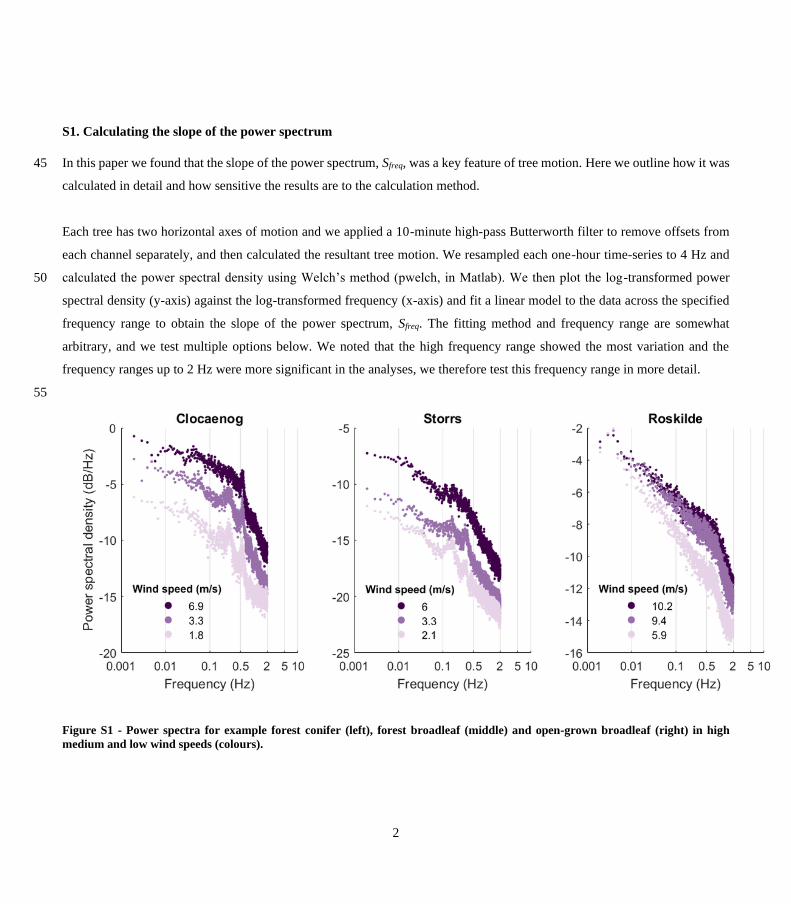
S1. Calculating the slope of the power spectrum

In this paper we found that the slope of the power spectrum, Sfreq, was a key feature of tree motion. Here we outline how it was 45

calculated in detail and how sensitive the results are to the calculation method.

Each tree has two horizontal axes of motion and we applied a 10-minute high-pass Butterworth filter to remove offsets from

each channel separately, and then calculated the resultant tree motion. We resampled each one-hour time-series to 4 Hz and

calculated the power spectral density using Welch’s method (pwelch, in Matlab). We then plot the log-transformed power 50

spectral density (y-axis) against the log-transformed frequency (x-axis) and fit a linear model to the data across the specified

frequency range to obtain the slope of the power spectrum, Sfreq. The fitting method and frequency range are somewhat

arbitrary, and we test multiple options below. We noted that the high frequency range showed the most variation and the

frequency ranges up to 2 Hz were more significant in the analyses, we therefore test this frequency range in more detail.

55

Figure S1 - Power spectra for example forest conifer (left), forest broadleaf (middle) and open-grown broadleaf (right) in high

medium and low wind speeds (colours).

3

We tested two methods to fit linear models to the power spectra: (1) using the output of pwelch directly and (2) logarithmically 60

re-sampling the output to give evenly distributed log-transformed data. We found that this re-sampling altered the absolute

values of the slope slightly, but did not alter the observed trends.

Figure S2 - Linear models of the power spectra to calculate slope using output of pwelch directly (left) and logarithmically re-

sampled output (right). The frequency interval used in the above is 0.3 - 2 Hz. 65

We tested three frequency intervals over which to fit the linear models, 0.05-2, 0.3-2 and 1-2 Hz. The first two intervals

produced similar trends with slightly different absolute values. The shortest interval had a similar trend but was partially

obscured by an increased level of noise.

70

4

Figure S3 - Slope of the power spectrum against wind speed for three example trees (same as Figure S1) for three different frequency

ranges.

75

Figure S4 – Same as figure S3 but calculated using the logarithmically re-sampled power spectrum output.

Overall, we find that the trend described in Figure 4d of the main text is robust to the different frequency ranges and fitting

methods.

We also tested the effect of the Butterworth high-pass filter on the power spectra. The purpose of this filter is to remove offsets 80

in the tree motion data. These offsets vary slowly so we chose a 10-minute high-pass filter. We found this had no significant

effect on the power spectrum in the region of interest (0.05-2 Hz).

5

Figure S5 – Time-series for the same three trees as figures S1, 3 and 4 with and without the Butterworth high-pass filter. 85

S2. Example power spectra at original resolution 90

In the following we provide power spectra of tree motion (colours) and locally measured wind speed time-series (black) for

the sites in which we have sufficient data. These are the forest broadleaf trees (figure S5) and forest conifers (figure S6). These

power spectra were calculated at the original sampling frequency (all analysis in the main text was re-sampled to 4Hz) and we

therefore pre-multiplied the y-axes by the frequency to allow a direct comparison between sites. 95

6

Figure S6 – power spectra for hourly samples of tree motion data (coloured lines) and wind speeds (black lines) at high, medium

and low wind speed. Y-axis labels are the site names. The y-axis can be thought of as a measure of the relative energy content, in

arbitrary units. The red dashed lines show the -2/3 slope as a reference point. The right-hand panels shows the difference between 100 high and low wind speeds and the horizontal dashed line represents 0 change. Numbers in the top right-hand corners show the mean

hourly wind speeds for the data sample. All of these sites are forest broadleaf trees.

105

7

Figure S7 - Same as figure S6 but for sites in conifer forests.

110

115

8

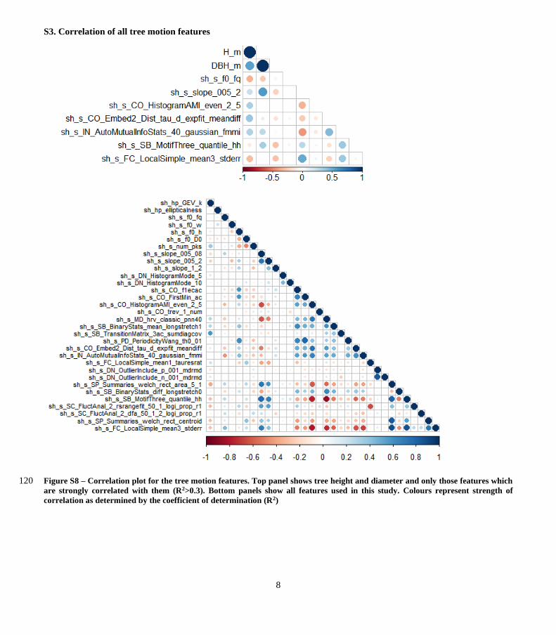
S3. Correlation of all tree motion features

Figure S8 – Correlation plot for the tree motion features. Top panel shows tree height and diameter and only those features which 120 are strongly correlated with them (R2>0.3). Bottom panels show all features used in this study. Colours represent strength of

correlation as determined by the coefficient of determination (R2)

9

S4. Correlation between tree size and tree motion features 125

We considered a subset of trees (N=168, 86 forest broadleaves, 54 forest conifers and 28 open-grown broadleaves) for which

height, dbh and tree motion data were available. In order to test which features were closely related to tree size, while

accounting for tree types, we predicted tree height and diameter from the tree motion features using a multiple linear regression

including tree type in the model as a factor (Table 3). The best single predictor of dbh was Sfreq while 𝑓0 was the second best

predictor of tree height after a catch22 feature (CO_Embed2_Dist_tau_d_expfit_meandiff). The factor “tree type” was the 9th 130

most explanatory feature in the model of height and 6th in the model of dbh. This demonstrates that tree size is more strongly

related to tree motion features than it is to tree type. Therefore, the relationship between tree type and tree motion features is

unlikely to be confounded by differences in tree size, and hence the results of our classification analyses are valid.

Model for DBH R2 AIC

Power spectral slope (𝑆𝑓𝑟𝑒𝑞) 0.05 – 2 Hz 0.308 174

IN_AutoMutualInfoStats_40_gaussian_fmmi 0.356 163

CO_FirstMin_ac 0.396 152

SB_MotifThree_quantile_hh 0.426 144

FC_LocalSimple_mean3_stderr 0.477 128

DN_OutlierInclude_p_001_mdrmd 0.494 123

Power spectral slope (𝑆𝑓𝑟𝑒𝑞) 1 – 2 Hz 0.509 119

CO_f1ecac 0.530 111

Tree type 0.546 108 135

Table S1 - Summary statistics from the most parsimonious multiple linear models relating tree DBH to tree motion features. Each

feature is added to the model sequentially in order of the largest decrease in AIC. A brief description of the catch22 features can be

found in the next section (S5) and a more detailed description in the associated publication (Lubba et al 2019).

140

145

10

Model for height R2 AIC

CO_Embed2_Dist_tau_d_expfit_meandiff 0.127 1272

Fundamental frequency (𝑓0) 0.194 1259

SB_TransitionMatrix_3ac_sumdiagcov 0.236 1250

Power spectral slope (𝑆𝑓𝑟𝑒𝑞) 0.05 – 2 Hz 0.286 1239

PD_PeriodicityWang_th0_01 0.318 1232

Number of wavelet peaks 0.329 1230

Tree type 0.353 1226

SP_Summaries_welch_rect_centroid 0.364 1224

CO_HistogramAMI_even_2_5 0.385 1219

150

Table S2 - Summary statistics from the most parsimonious multiple linear models relating tree height to tree motion features. Each

feature is added to the model sequentially in order of the largest decrease in AIC. A brief description of the catch22 features can be

found in the supplementary materials (S4) and a more detailed description in the associated publication (Lubba et al 2019).

S5. Catch22 features table

155

11

160

Name Description

a DN_HistogramMode_5 Mode of z-scored distribution (5-bin histogram)

b DN_HistogramMode_10 Mode of z-scored distribution (10-bin histogram)

c SB_BinaryStats_mean_longstretch1 Longest period of consecutive values above the mean

d DN_OutlierInclude_p_001_mdrmd

Time intervals between successive extreme events above the

mean

e DN_OutlierInclude_n_001_mdrmd

Time intervals between successive extreme events below the

mean

f CO_f1ecac First 1/e crossing of autocorrelation function

g CO_FirstMin_ac First minimum of autocorrelation function

h SP_Summaries_welch_rect_area_5_1

Total power in lowest fifth of frequencies in the Fourier power

spectrum

i SP_Summaries_welch_rect_centroid Centroid of the Fourier power spectrum

j FC_LocalSimple_mean3_stderr Mean error from a rolling 3-sample mean forecasting

k CO_trev_1_num Time-reversibility statistic, h(xt+1 − xt)3it

l CO_HistogramAMI_even_2_5 Automutual information, m = 2, = 5

m IN_AutoMutualInfoStats_40_gaussian_fmmi First minimum of the automutual information function

n MD_hrv_classic_pnn40 Proportion of successive differences exceeding 0.04

o SB_BinaryStats_diff_longstretch0 Longest period of successive incremental decreases

p SB_MotifThree_quantile_hh

Shannon entropy of two successive letters in equiprobable 3-

letter symbolization

q FC_LocalSimple_mean1_tauresrat Change in correlation length after iterative differencing

r CO_Embed2_Dist_tau_d_expfit_meandiff Exponential fit to successive distances in 2-d embedding space

s SC_FluctAnal_2_dfa_50_1_2_logi_prop_r1

Proportion of slower timescale fluctuations that scale with DFA

(50% sampling)

t SC_FluctAnal_2_rsrangefit_50_1_logi_prop_r1

Proportion of slower timescale fluctuations that scale with

linearly rescaled range fits

u SB_TransitionMatrix_3ac_sumdiagcov

Trace of covariance of transition matrix between symbols in 3-

letter alphabet

v PD_PeriodicityWang_th0_01

Periodicity measure of Wang, X., Wirth, A., Wang, L.:

Structure-based statistical features and multivariate

time series clustering. Proceedings - IEEE International

Conference on Data Mining,

ICDM pp. 351–360 (2007).