Supplement of The AeroCom evaluation and …€¦ · 2 CMU-VBS calculates that almost all POC has undergone aging, ... 20 CAM4-Oslo has a mPOA source ... are presented in the Supplement

Supplement of Atmos. Chem. Phys., 14, 10845–10895, 2014http://www.atmos-chem-phys.net/14/10845/2014/doi:10.5194/acp-14-10845-2014-supplement© Author(s) 2014. CC Attribution 3.0 License.

Supplement of

The AeroCom evaluation and intercomparison of organic aerosol inglobal models

K. Tsigaridis et al.

Correspondence to:K. Tsigaridis ([email protected]) and M. Kanakidou ([email protected])

4

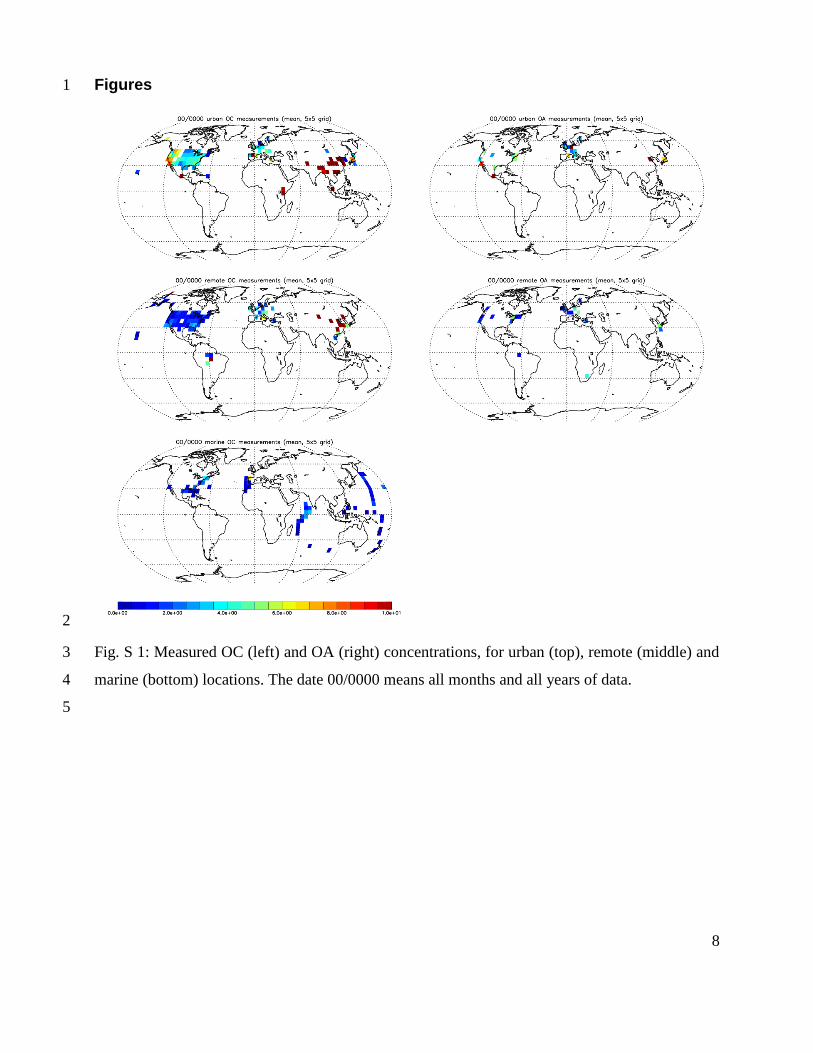
All measurements used in the present study are visualized in Fig. S 1, interpolated in a 5°x5° grid 1

in Fig. S 2 and the total count of data per 5°x5° grid in Fig. S 3. 2

The median, 25/75% and 9/91% of POA emissions, SOA chemical production and total OA sources 3

(POA emissions + SOA chemical production), as well as their normalized seasonal variability per 4

model, are presented in Fig. S 4. Similarly, the POA/SOA/OA load is presented in Fig. S 5, the 5

dry/wet OA deposition in Fig. S 6, the POA/SOA/OA lifetime in Fig. S 7, and the clear-sky AOD 6

at 550 nm in Fig. S 8. 7

The annual mean OA surface concentration by all models is presented in Fig. S 9, the scatterplot 8

between modeled and measured OC in Fig. S 10 and for OA in Fig. S 11. 9

The seasonal variability of OC chemical composition for the models not presented in the main 10

paper are shown in Fig. S 12 for Finokalia, Greece (remote), Fig. S 13 for Welgegung, South Africa 11

(remote), Fig. S 14 for Alaska, USA (remote), Fig. S 15 for Manaus, Brazil (remote), and Fig. S 12

16 for Amsterdam Island, Indian Ocean (marine). Also presented are the seasonal variability of the 13

OA chemical composition for the models not presented in the main paper in Fig. S 17 for Finokalia, 14

Greece (remote), Fig. S 18 for Welgegung, South Africa (remote), Fig. S 19 for Alaska, USA 15

(remote), Fig. S 20 for Manaus, Brazil (remote), and Fig. S 21 for Amsterdam Island, Indian Ocean 16

(marine). 17

In addition to the stations mentioned above, we discuss here a few additional stations. These are 18

presented in the same way as in the main paper: First their seasonal variability and the chemical 19

composition as calculated by the five models discussed in the paper, and then the calculated 20

chemical composition from the remaining ones. 21

The models are neither expected to, nor are able to capture the aerosol mass concentrations 22

measured at urban stations. They are expected, though, and are able to, perform much better at 23

remote stations, even in the vicinity of urban stations, as long as the urban plume does not 24

significantly affect the remote station measurements. The models calculate very similar aerosol 25

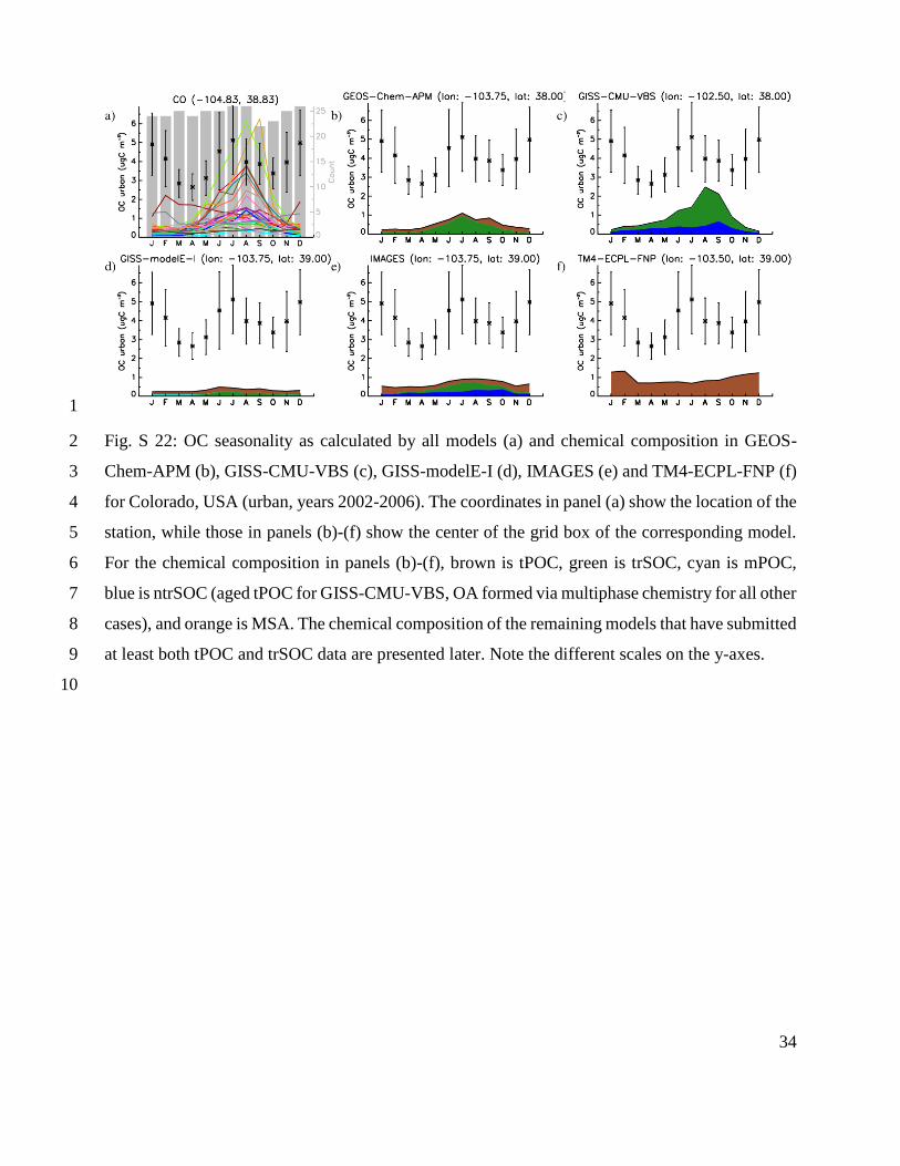
levels and OA chemical composition in Colorado, USA, both over an urban station (Fig. S 22) and 26

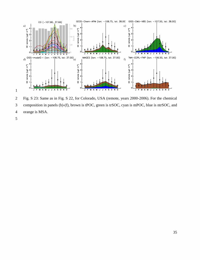
a remote one (Fig. S 23). Since the remote station is surrounded by forests, the contribution of the 27

(mostly biogenically formed) trSOC is present year-round. During summer, most models calculate 28

that trSOC dominates the total OC in that area, with contributions approaching 100% of the total 29

5

OC. Multiphase chemistry also contributes significant amounts of aerosols to the total OC. GISS-1

CMU-VBS calculates that almost all POC has undergone aging, even at the urban station, probably 2

due to the very coarse model grid that does not resolve the urban core and makes the contribution 3

of the fresh urban emissions appear insignificant. CCSM4-Chem, ECHAM5-HAM2, GEOS-4

Chem-APM and TM4-ECPL-FNP appear to calculate a higher contribution of tPOC to the total 5

OC levels; in the latter model case, this is due to the presence of primary biological particle 6

emissions. SPRINTARS, which has a very fine grid, simulates virtually all OC as trSOC at the 7

remote station, while tPOC dominates during winter at the urban station, presumably due to high 8

anthropogenic emissions that are resolved on the fine grid of that model. The same can be seen 9

with the coarser grid CCSM4-Chem model, but to a lesser extent. 10

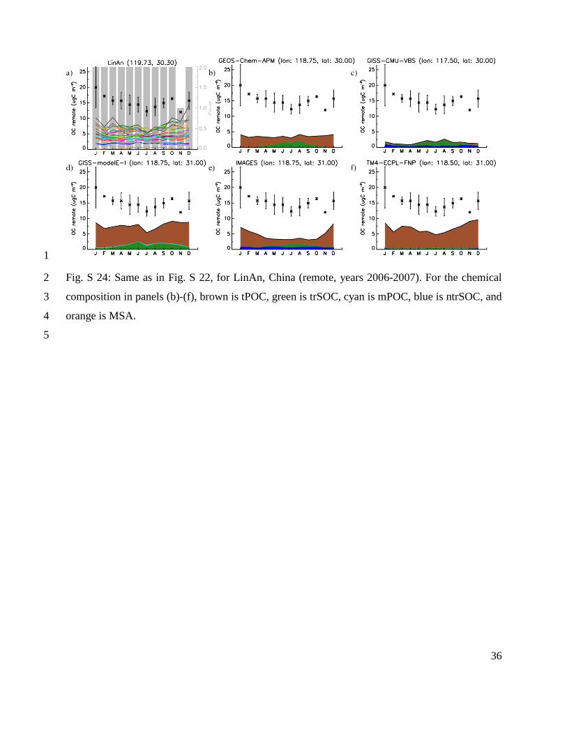
The OA concentrations at the remote station LinAn, China (Fig. S 24), are underestimated by the 11

models. All models calculate a high contribution of tPOC to the total OC levels, a clear indication 12

of very strong regional anthropogenic pollution. Not all models agree on the trSOC contribution to 13

the total OC, with about half of the models that resolve the OC chemical composition calculating 14

a contribution that approaches 50% during summer, and the other half calculating a much smaller 15

contribution. IMPACT and IMAGES suggest that a significant amount of OC comes from 16

multiphase chemistry, while the two TM4-ECPL models do not. Recall that TM4-ECPL has a more 17

detailed aqueous chemistry scheme than the other two models, which probably explains the 18

difference in the results. 19

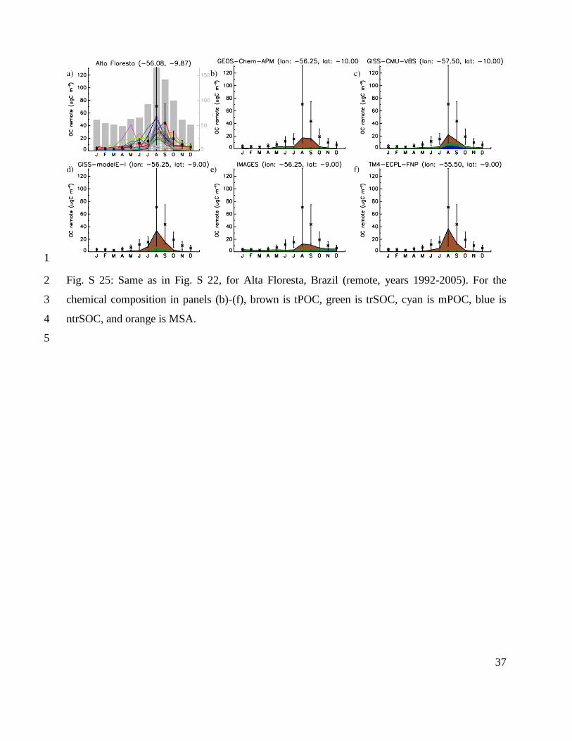
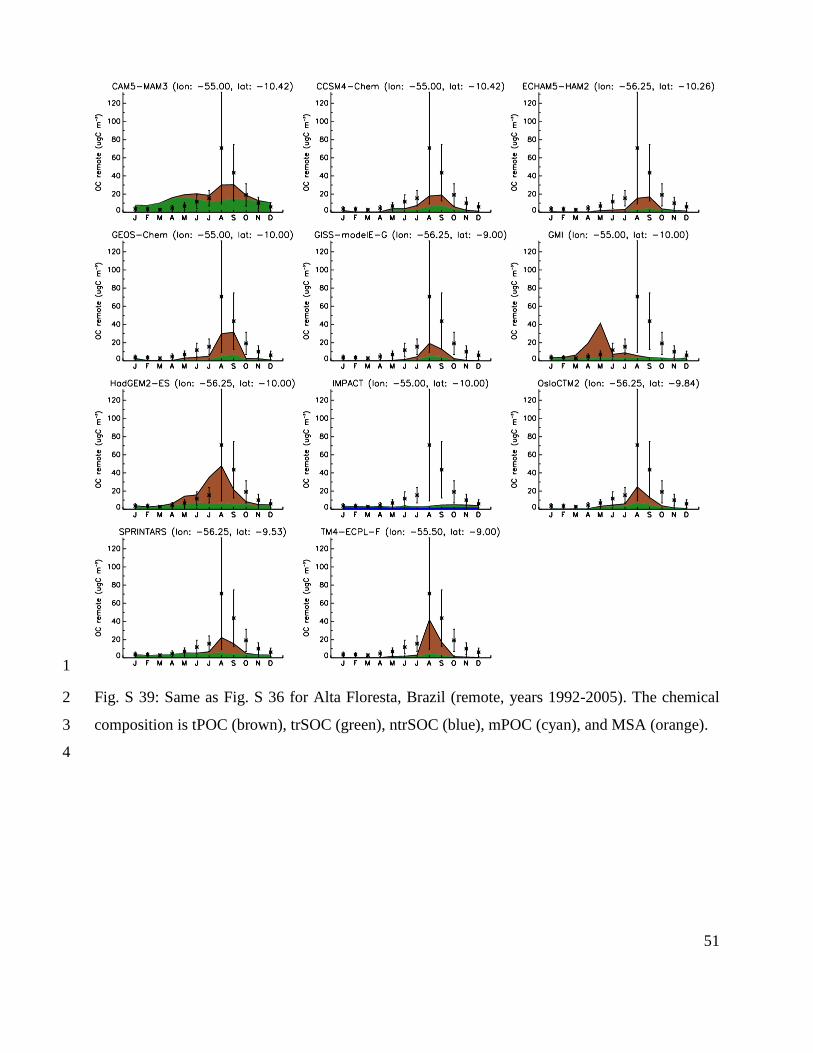
A region where biomass burning is also important is the Amazon basin. Alta Floresta, Brazil (Fig. 20

S 25), is a site with very long-term measurements and a clear biomass burning peak during the dry 21

season, which the models reproduce quite successfully, with the exception of GMI that peaks 22

during May. Two other models, BCC and IMPACT, do not capture the dry season peak, which 23

shows potential problems with their biomass burning emissions in the region. Care has to be taken 24

regarding the year simulated and compared with measurements. Through the years Alta Floresta 25

has experienced a significant reduction in biomass burning intensity in the region, while the data 26

shown in are the climatology of all years of measurements. During the biomass burning period, 27

GISS-CMU-VBS simulates equal amounts of fresh and aged POA, reflecting the close vicinity of 28

POA sources. Multiphase chemistry appears not to play a significant role here, in contrast with the 29

Manaus station, Brazil (Fig. 22), where IMPACT and IMAGES calculate significant amounts of 30

6

ntrSOA; the location of the inter-tropical convergence zone (ITCZ) and the potentially very 1

different availability of cloud and aerosol water at these stations appears to be the reason behind 2

this important difference. At the same station, many models also calculate large amounts of trSOA 3

during the dry season. 4

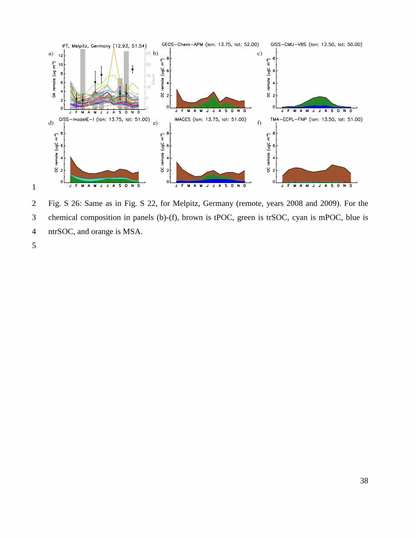
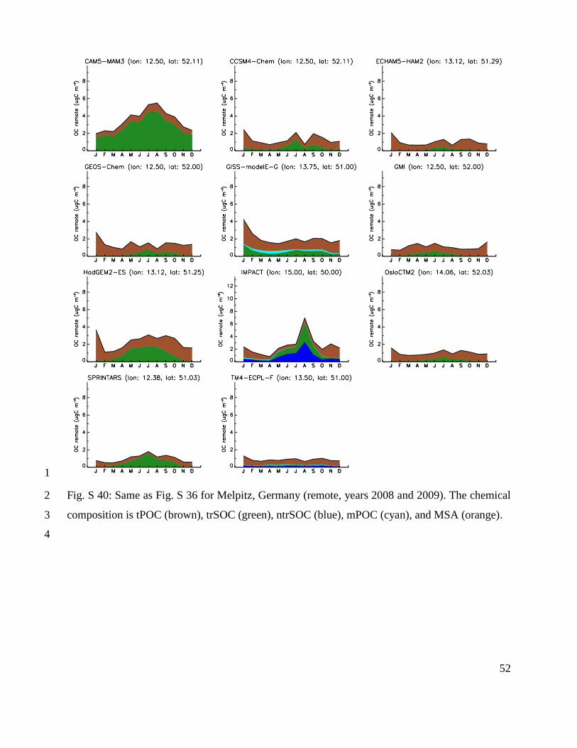
In Melpitz, Germany (Fig. S 26), most models agree that there is no clear seasonality, other than a 5

winter and a weak summer peak. The measurements do not present a clear seasonality either, 6

although the spread of the concentrations is larger than that calculated by most models, and there 7

are gaps in the data that make the comparison more difficult. In any case, emissions during winter 8

appear to be significant, although fossil fuel emissions from different models are not the same (e.g. 9

IMPACT vs. TM4-ECPL-F, where the models calculate very similar distributions with different 10

absolute amounts due to different emission inventories). GISS-CMU-VBS has almost no POA, 11

either fresh or aged; the calculated OA is mostly trSOA, which is present during summer in the 12

models. Multiphase chemistry also forms a significant fraction of the total OC. TM4-ECPL-FNP 13

calculates a high contribution from primary biological particles, but its seasonality does not agree 14

with that of the measurements. 15

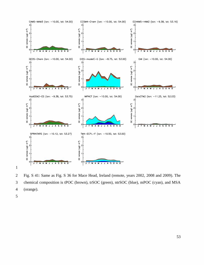
The Mace Head station on the west coast of Ireland (Fig. S 27) receives mostly oceanic air masses. 16

Among the models that include an mPOA source, GISS-modelE-G/I and IMPACT exceed the 17

measured OA, except a high value in May, which might be either an outlier or something related 18

to a source that the models are unable to capture. Among the other models that include mPOA, 19

CAM4-Oslo has a mPOA source (added to tPOA) that follows the offline sea salt fluxes from 20

AeroCom phase I (not the ones calculated online in the model) and TM4-ECPL-F/FNP have a low 21

global flux; these models are closer to the measurements than the rest of the models that include 22

mPOA. The models that do not include any mPOA parameterization calculate much lower OA 23

concentrations. Products from multiphase chemistry are also present, while primary anthropogenic 24

and biomass burning aerosols are virtually absent. Caution has to be taken because Mace Head is 25

at the coast; many models that have their gridbox edge at 10°W use a continental box for 26

representing Mace Head (longitude 9.9°W), which might not be representative for its 27

predominantly marine environment. 28

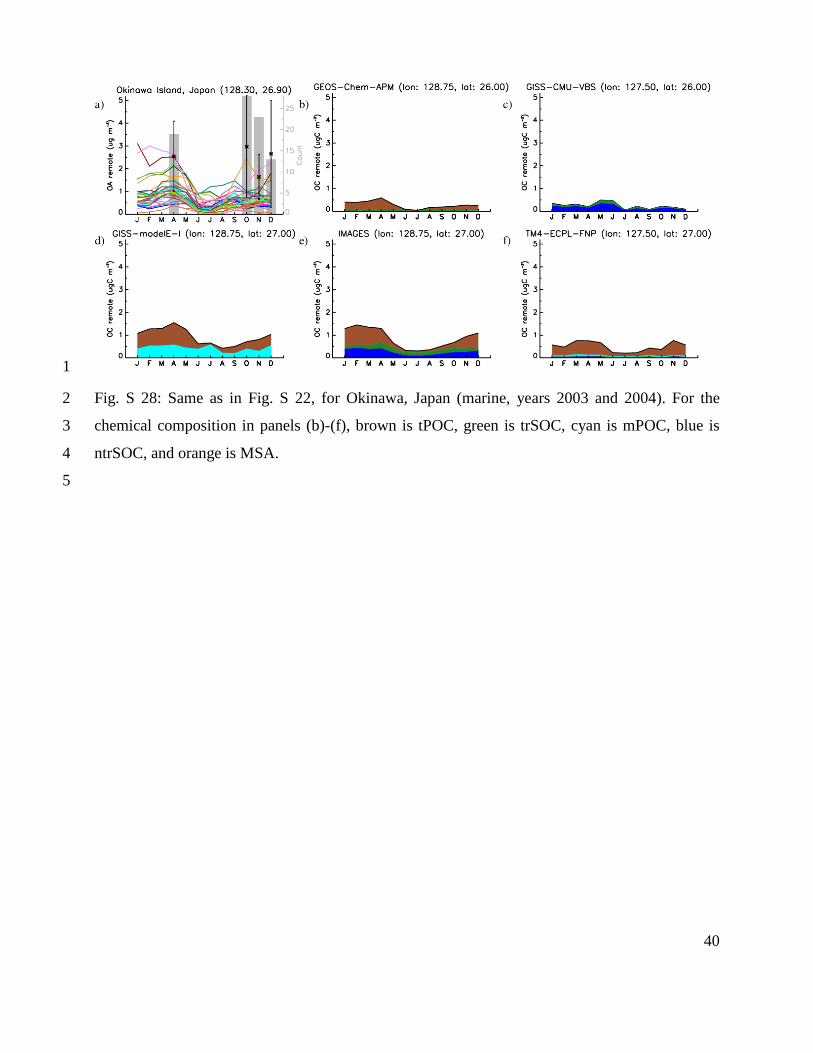
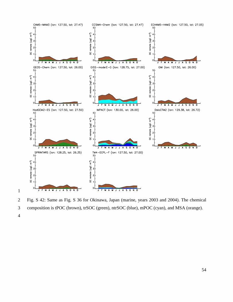
Okinawa, Japan (Fig. S 28), is a remote marine site that is influenced by long-range transport of 29

pollution aerosol from East Asia. AMS measurements at four different months suggest that 2-3 ug 30

7

m-3 are present over Okinawa, an amount that only models that include either multiphase chemistry 1

of organics, or mPOA sources, or both, can reproduce. IMAGES appears to agree best with 2

measurements, and the two TM4-ECPL models, although having both ntrSOA and mPOA, are 3

rather low. All models agree that there is a minimum in OA concentrations during summer, but 4

unfortunately no data are available to validate this trend. Small but significant OA amounts come 5

from multiphase chemistry. The models also calculate an important contribution of very aged POA. 6

The OA chemical composition from the AMS perspective for the above mentioned stations for five 7

models (as presented in the main text) is shown in Fig. S 29 for Colorado, USA (urban), Fig. S 30 8

for Colorado, USA (remote), Fig. S 31 for LinAn, China (remote), Fig. S 32 for Alta Floresta, 9

Brazil (remote), Fig. S 33 for Melpitz, Germany (remote), Fig. S 34 for Mace Head, Ireland 10

(remote), and Fig. S 35 for Okinawa, Japan (marine). In addition, the chemical composition for the 11

remaining models that have more than one organic aerosol tracer are presented for OC in Fig. S 36 12

for Colorado, USA (urban), Fig. S 37 for Colorado, USA (remote), Fig. S 38 for LinAn, China 13

(remote), Fig. S 39 for Alta Floresta, Brazil (remote), Fig. S 40 for Melpitz, Germany (remote), 14

Fig. S 41 for Mace Head, Ireland (remote), and Fig. S 42 for Okinawa, Japan (marine), and for OA 15

in Fig. S 43 for Colorado, USA (urban), Fig. S 44 for Colorado, USA (remote), Fig. S 45 for LinAn, 16

China (remote), Fig. S 46 for Alta Floresta, Brazil (remote), Fig. S 47 for Melpitz, Germany 17

(remote), Fig. S 48 for Mace Head, Ireland (remote), and Fig. S 49 for Okinawa, Japan (marine). 18

19

8

Figures 1

2

Fig. S 1: Measured OC (left) and OA (right) concentrations, for urban (top), remote (middle) and 3

marine (bottom) locations. The date 00/0000 means all months and all years of data. 4

5

9

1

Fig. S 2: Mean measured OC (μgC m-3; left) and OA (μg m-3; right) concentrations on a 5°x5° 2

degree grid for urban (top), remote (middle) and marine (bottom) locations. The number of data 3

points per grid cell, as well as the individual stations, are presented in the Supplement. The date 4

00/0000 means all months and all years of data. 5

6

10

1

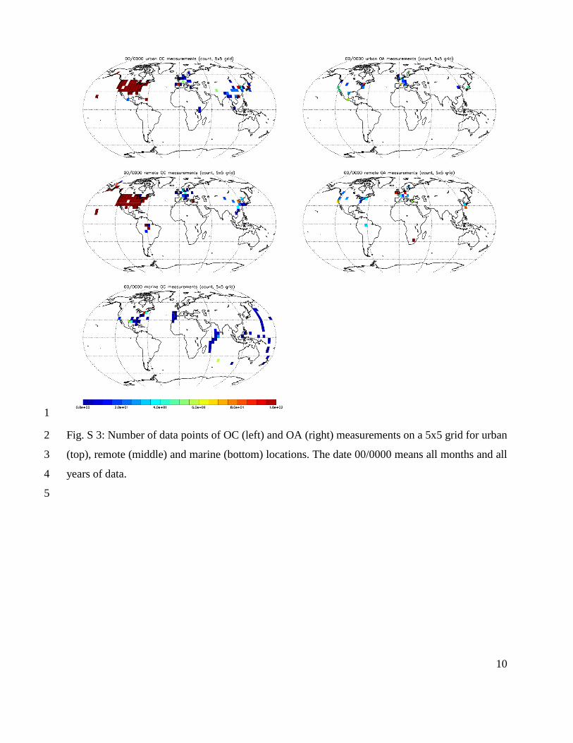
Fig. S 3: Number of data points of OC (left) and OA (right) measurements on a 5x5 grid for urban 2

(top), remote (middle) and marine (bottom) locations. The date 00/0000 means all months and all 3

years of data. 4

5

11

1

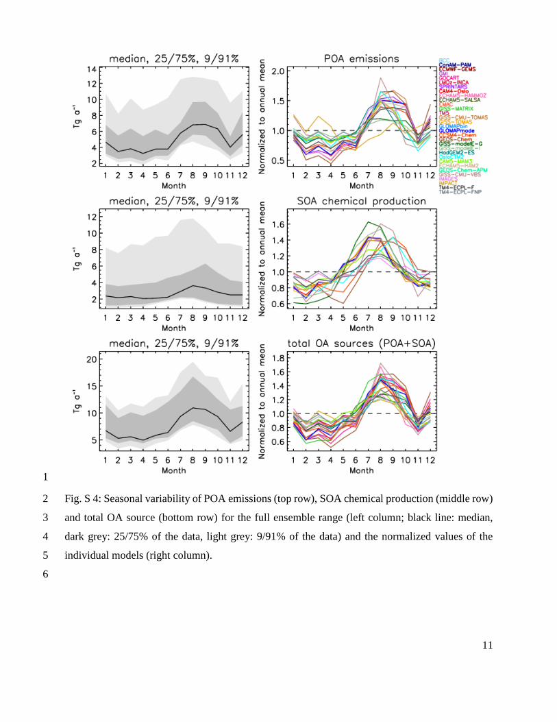
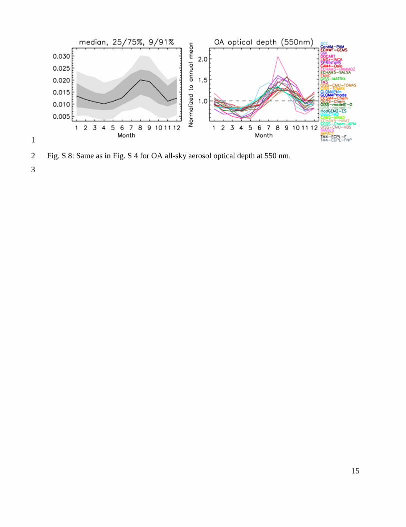
Fig. S 4: Seasonal variability of POA emissions (top row), SOA chemical production (middle row) 2

and total OA source (bottom row) for the full ensemble range (left column; black line: median, 3

dark grey: 25/75% of the data, light grey: 9/91% of the data) and the normalized values of the 4

individual models (right column). 5

6

12

1

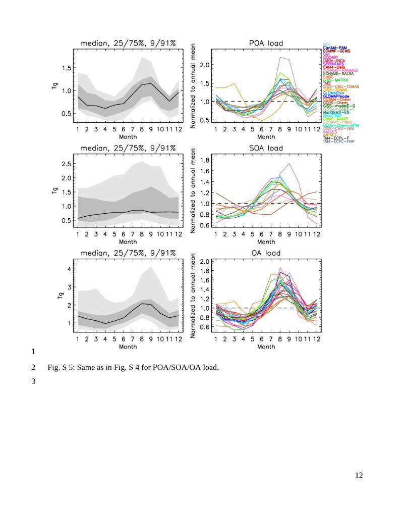
Fig. S 5: Same as in Fig. S 4 for POA/SOA/OA load. 2

3

13

1

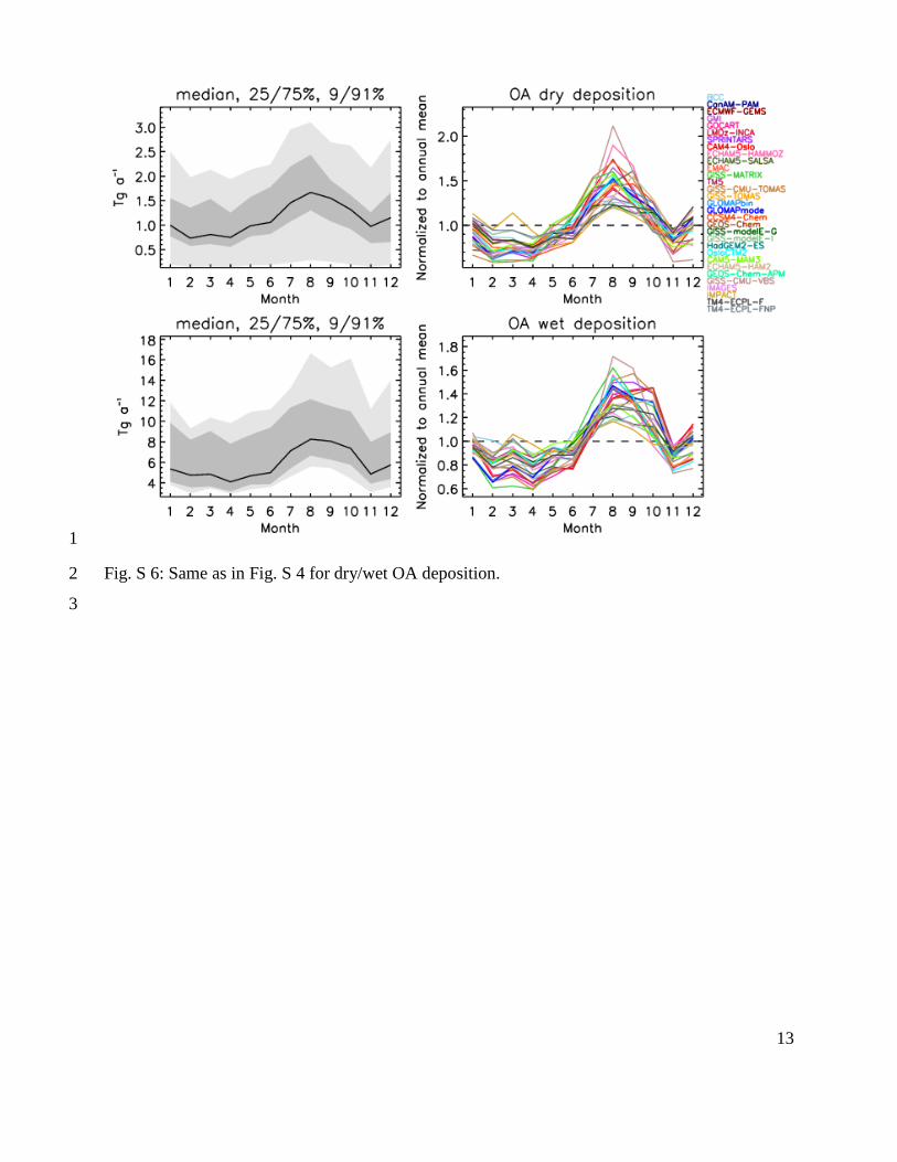
Fig. S 6: Same as in Fig. S 4 for dry/wet OA deposition. 2

3

14

1

Fig. S 7: Same as in Fig. S 4 for POA/SOA/OA lifetime. 2

3

15

1

Fig. S 8: Same as in Fig. S 4 for OA all-sky aerosol optical depth at 550 nm. 2

3

16

1

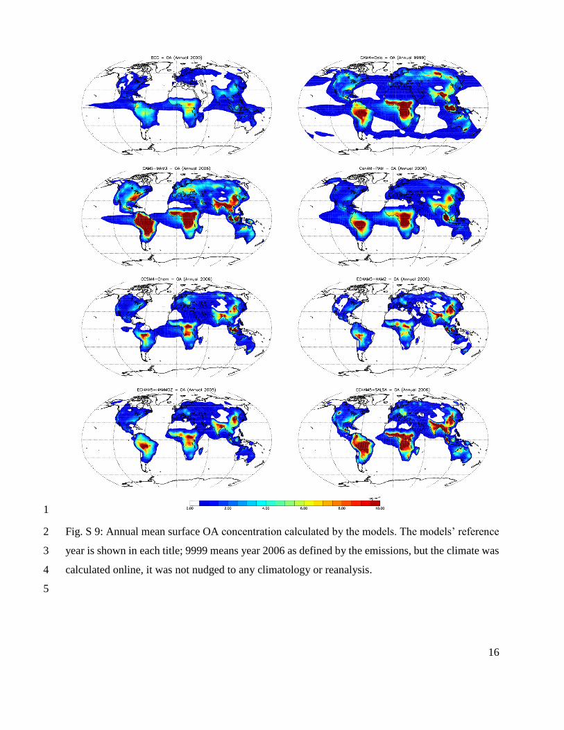
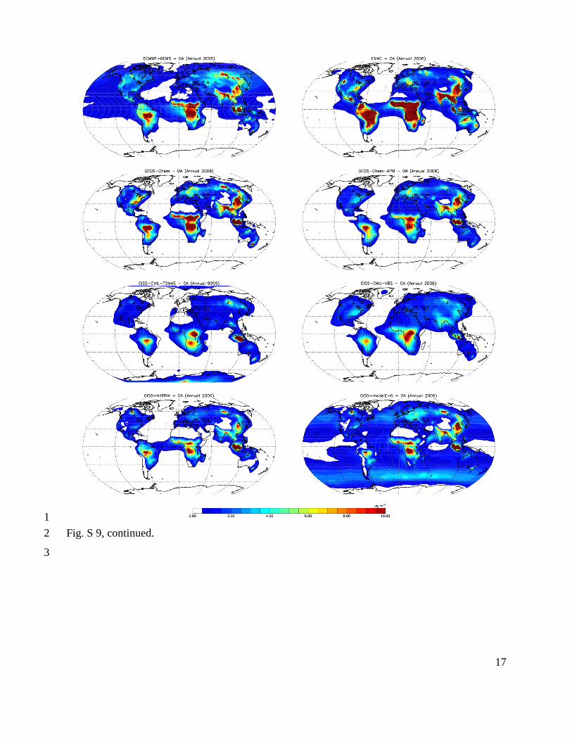
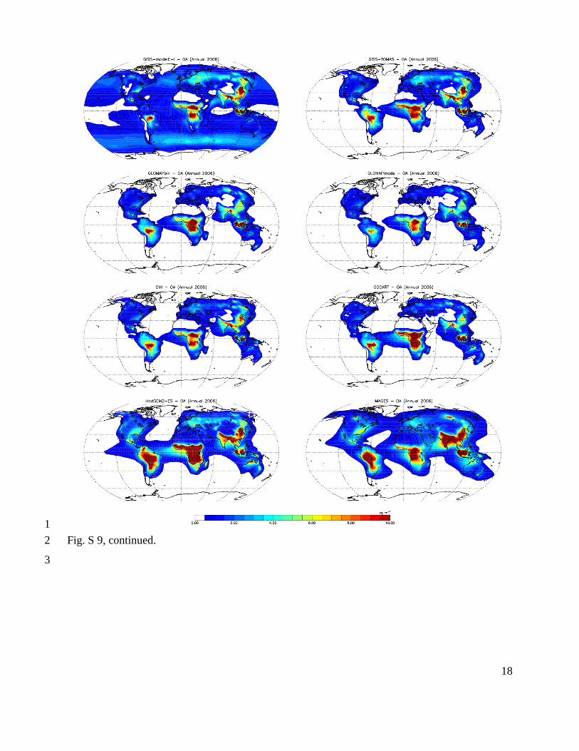
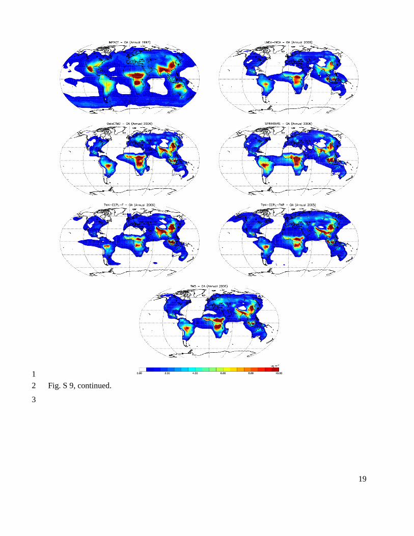
Fig. S 9: Annual mean surface OA concentration calculated by the models. The models’ reference 2

year is shown in each title; 9999 means year 2006 as defined by the emissions, but the climate was 3

calculated online, it was not nudged to any climatology or reanalysis. 4

5

17

1

Fig. S 9, continued. 2

3

18

1


3

19

1


3

20

1

Fig. S 10: Comparison of model results with OC measurements. Stations are marked by color: 2

urban (brown), remote (green), marine (blue). The year in parenthesis next to the model name 3

denotes the simulated year. 4

5

21

1


3

22

1

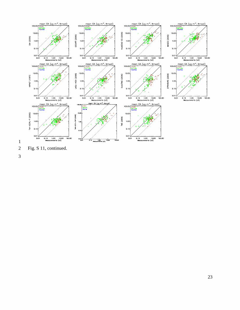
Fig. S 11: Same as Fig. S 10 for OA measurements. 2

3

23

1


3

24

1

2

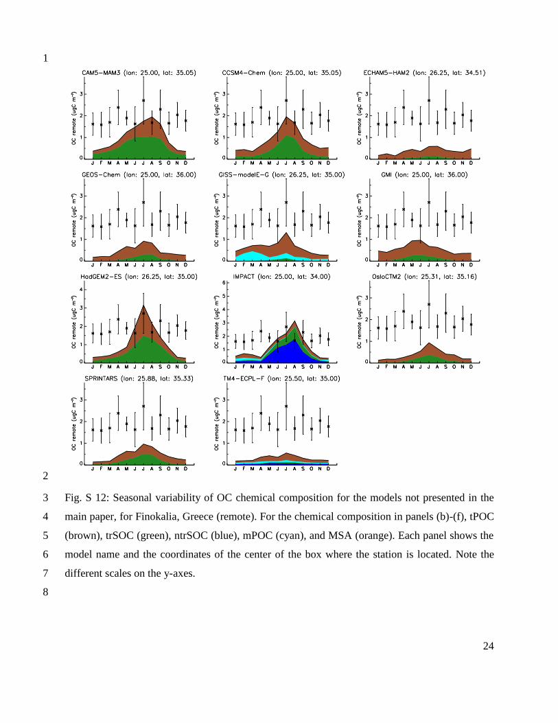
Fig. S 12: Seasonal variability of OC chemical composition for the models not presented in the 3

main paper, for Finokalia, Greece (remote). For the chemical composition in panels (b)-(f), tPOC 4

(brown), trSOC (green), ntrSOC (blue), mPOC (cyan), and MSA (orange). Each panel shows the 5

model name and the coordinates of the center of the box where the station is located. Note the 6

different scales on the y-axes. 7

8

25

1

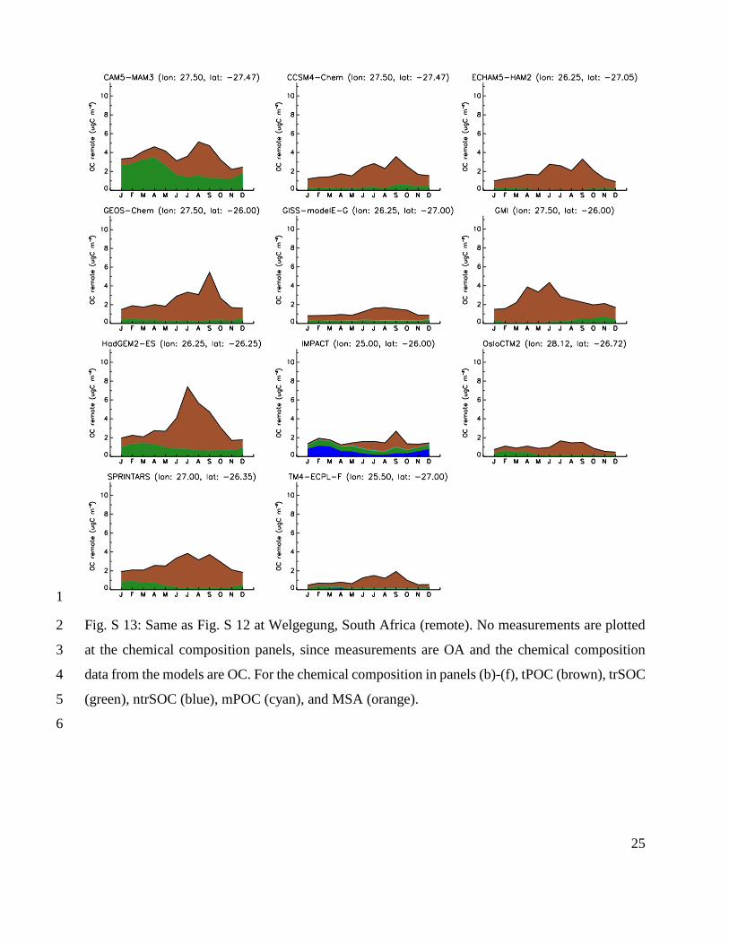
Fig. S 13: Same as Fig. S 12 at Welgegung, South Africa (remote). No measurements are plotted 2

at the chemical composition panels, since measurements are OA and the chemical composition 3

data from the models are OC. For the chemical composition in panels (b)-(f), tPOC (brown), trSOC 4

(green), ntrSOC (blue), mPOC (cyan), and MSA (orange). 5

6

26

1

Fig. S 14: Same as Fig. S 12 for Alaska, USA (remote). For the chemical composition in panels 2

(b)-(f), tPOC (brown), trSOC (green), ntrSOC (blue), mPOC (cyan), and MSA (orange). 3

4

27

1

Fig. S 15: Same as Fig. S 12 for Manaus, Brazil (remote). For the chemical composition in panels 2

(b)-(f), tPOC (brown), trSOC (green), ntrSOC (blue), mPOC (cyan), and MSA (orange). 3

4

28

1

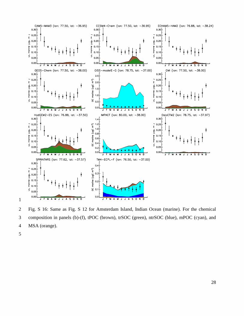
Fig. S 16: Same as Fig. S 12 for Amsterdam Island, Indian Ocean (marine). For the chemical 2

composition in panels (b)-(f), tPOC (brown), trSOC (green), ntrSOC (blue), mPOC (cyan), and 3

MSA (orange). 4

5

29

1

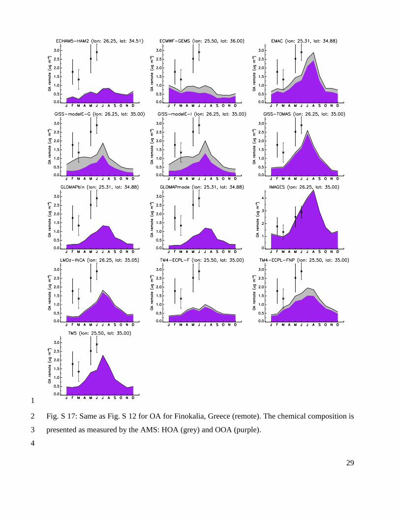
Fig. S 17: Same as Fig. S 12 for OA for Finokalia, Greece (remote). The chemical composition is 2

presented as measured by the AMS: HOA (grey) and OOA (purple). 3

4

30

1

Fig. S 18: Same as Fig. S 17 for Welgegung, South Africa (remote). The chemical composition is 2

presented as measured by the AMS: HOA (grey) and OOA (purple). 3

4

31

1

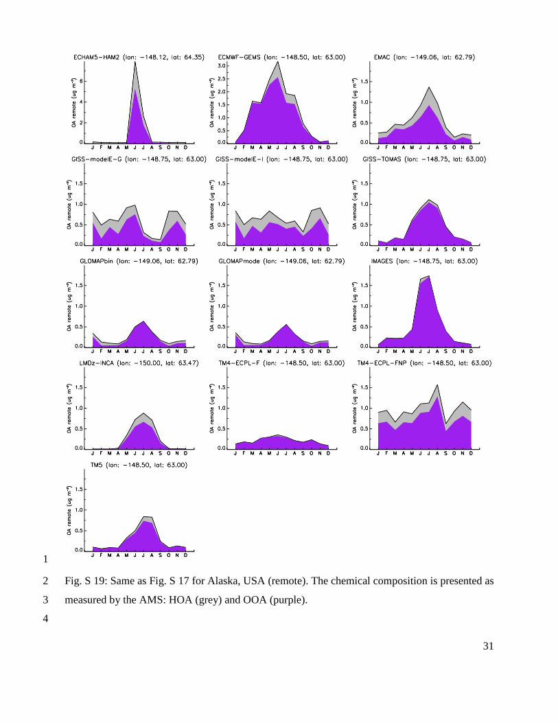
Fig. S 19: Same as Fig. S 17 for Alaska, USA (remote). The chemical composition is presented as 2

measured by the AMS: HOA (grey) and OOA (purple). 3

4

32

1

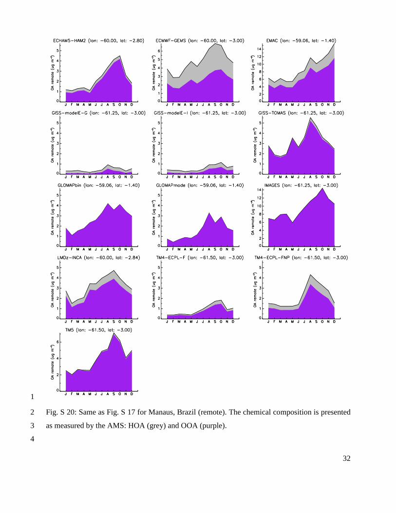
Fig. S 20: Same as Fig. S 17 for Manaus, Brazil (remote). The chemical composition is presented 2

as measured by the AMS: HOA (grey) and OOA (purple). 3

4

33

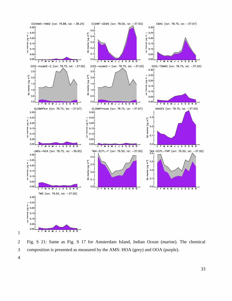
1

Fig. S 21: Same as Fig. S 17 for Amsterdam Island, Indian Ocean (marine). The chemical 2

composition is presented as measured by the AMS: HOA (grey) and OOA (purple). 3

4

34

1

Fig. S 22: OC seasonality as calculated by all models (a) and chemical composition in GEOS-2

Chem-APM (b), GISS-CMU-VBS (c), GISS-modelE-I (d), IMAGES (e) and TM4-ECPL-FNP (f) 3

for Colorado, USA (urban, years 2002-2006). The coordinates in panel (a) show the location of the 4

station, while those in panels (b)-(f) show the center of the grid box of the corresponding model. 5

For the chemical composition in panels (b)-(f), brown is tPOC, green is trSOC, cyan is mPOC, 6

blue is ntrSOC (aged tPOC for GISS-CMU-VBS, OA formed via multiphase chemistry for all other 7

cases), and orange is MSA. The chemical composition of the remaining models that have submitted 8

at least both tPOC and trSOC data are presented later. Note the different scales on the y-axes. 9

10

35

1

Fig. S 23: Same as in Fig. S 22, for Colorado, USA (remote, years 2000-2006). For the chemical 2

composition in panels (b)-(f), brown is tPOC, green is trSOC, cyan is mPOC, blue is ntrSOC, and 3

orange is MSA. 4

5

36

1

Fig. S 24: Same as in Fig. S 22, for LinAn, China (remote, years 2006-2007). For the chemical 2

composition in panels (b)-(f), brown is tPOC, green is trSOC, cyan is mPOC, blue is ntrSOC, and 3

orange is MSA. 4

5

37

1

Fig. S 25: Same as in Fig. S 22, for Alta Floresta, Brazil (remote, years 1992-2005). For the 2

chemical composition in panels (b)-(f), brown is tPOC, green is trSOC, cyan is mPOC, blue is 3

ntrSOC, and orange is MSA. 4

5

38

1

Fig. S 26: Same as in Fig. S 22, for Melpitz, Germany (remote, years 2008 and 2009). For the 2



5

39

1

Fig. S 27: Same as in Fig. S 22, for Mace Head, Ireland (remote, years 2002, 2008 and 2009). For 2

the chemical composition in panels (b)-(f), brown is tPOC, green is trSOC, cyan is mPOC, blue is 3


5

40

1

Fig. S 28: Same as in Fig. S 22, for Okinawa, Japan (marine, years 2003 and 2004). For the 2



5

41

1

Fig. S 29: Same as Fig. S 22 for OA for Colorado, USA (urban, years 2002-2006). The chemical 2

composition (where available) is presented as measured by the AMS: HOA (grey) and OOA 3

(purple). 4

5

42

1

Fig. S 30: Same as Fig. S 22 for OA for Colorado, USA (remote, years 2000-2006). The chemical 2


(purple). 4

5

43

1

Fig. S 31: Same as Fig. S 22 for OA for LinAn, China (remote, years 2006-2007). The chemical 2


(purple). 4

5

44

1

Fig. S 32: Same as Fig. S 22 for OA for Alta Floresta, Brazil (remote, years 1992-2005). The 2

chemical composition (where available) is presented as measured by the AMS: HOA (grey) and 3

OOA (purple). 4

5

45

1

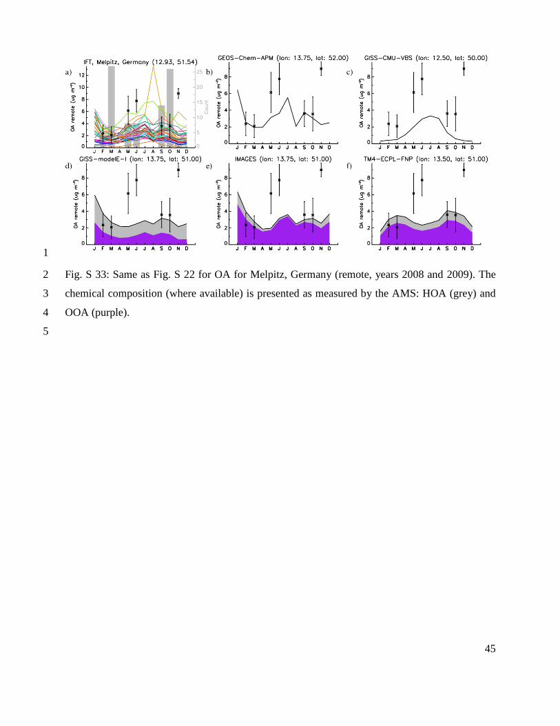
Fig. S 33: Same as Fig. S 22 for OA for Melpitz, Germany (remote, years 2008 and 2009). The 2


OOA (purple). 4

5

46

1

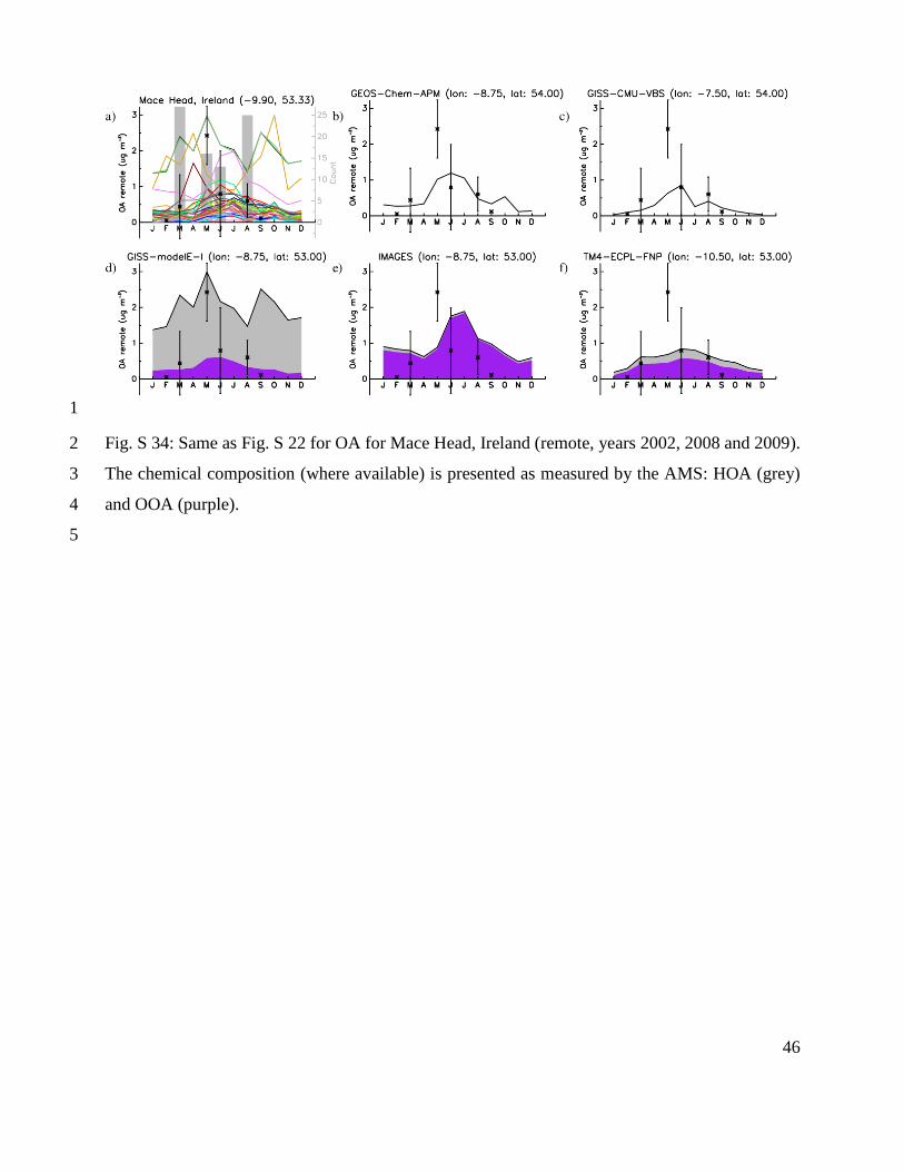
Fig. S 34: Same as Fig. S 22 for OA for Mace Head, Ireland (remote, years 2002, 2008 and 2009). 2

The chemical composition (where available) is presented as measured by the AMS: HOA (grey) 3

and OOA (purple). 4

5

47

1

Fig. S 35: Same as Fig. S 22 for OA for Okinawa, Japan (marine, years 2003 and 2004). The 2


OOA (purple). 4

5

48

1

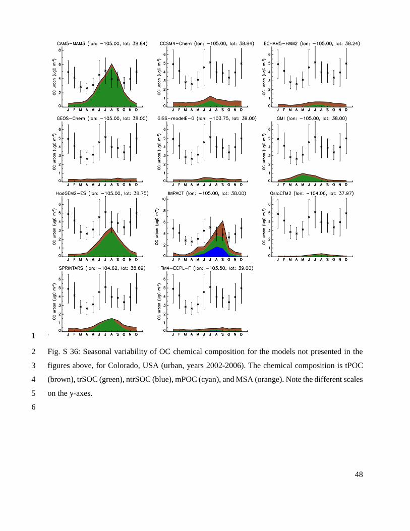
Fig. S 36: Seasonal variability of OC chemical composition for the models not presented in the 2

figures above, for Colorado, USA (urban, years 2002-2006). The chemical composition is tPOC 3

(brown), trSOC (green), ntrSOC (blue), mPOC (cyan), and MSA (orange). Note the different scales 4

on the y-axes. 5

6

49

1

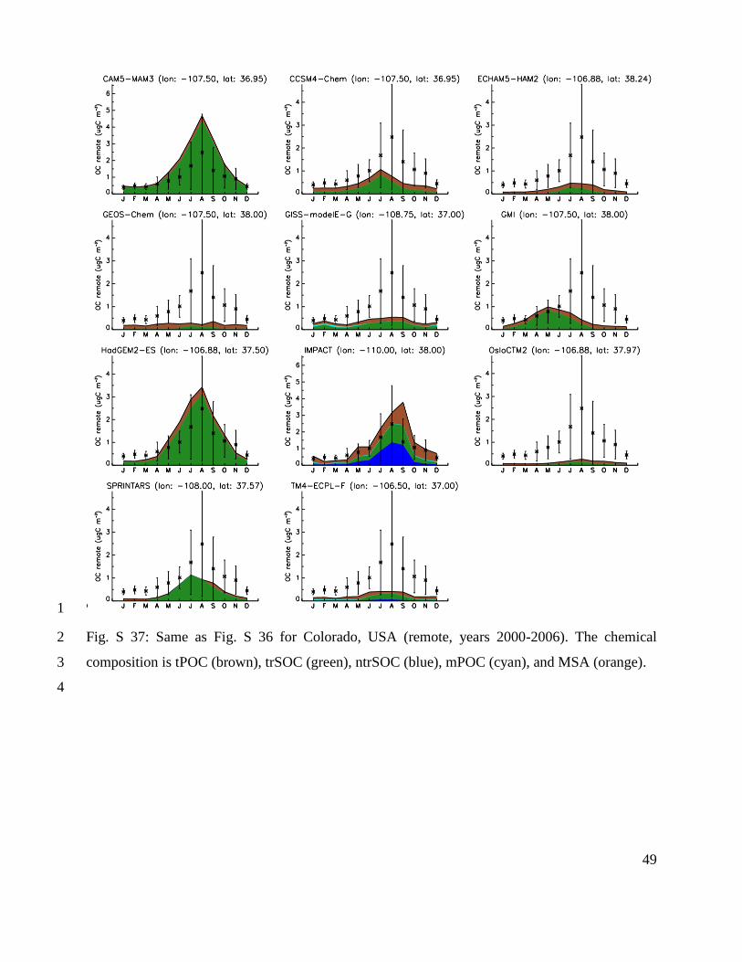
Fig. S 37: Same as Fig. S 36 for Colorado, USA (remote, years 2000-2006). The chemical 2

composition is tPOC (brown), trSOC (green), ntrSOC (blue), mPOC (cyan), and MSA (orange). 3

4

50

1

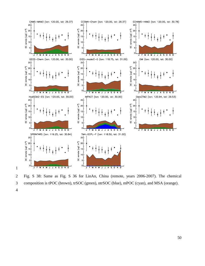
Fig. S 38: Same as Fig. S 36 for LinAn, China (remote, years 2006-2007). The chemical 2


4

51

1

Fig. S 39: Same as Fig. S 36 for Alta Floresta, Brazil (remote, years 1992-2005). The chemical 2


4

52

1

Fig. S 40: Same as Fig. S 36 for Melpitz, Germany (remote, years 2008 and 2009). The chemical 2


4

53

1

Fig. S 41: Same as Fig. S 36 for Mace Head, Ireland (remote, years 2002, 2008 and 2009). The 2

chemical composition is tPOC (brown), trSOC (green), ntrSOC (blue), mPOC (cyan), and MSA 3

(orange). 4

5

54

1

Fig. S 42: Same as Fig. S 36 for Okinawa, Japan (marine, years 2003 and 2004). The chemical 2


4

55

1

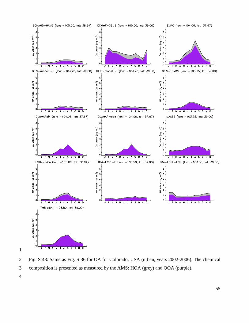
Fig. S 43: Same as Fig. S 36 for OA for Colorado, USA (urban, years 2002-2006). The chemical 2


4

56

1

Fig. S 44: Same as Fig. S 36 for OA for Colorado, USA (remote, years 2000-2006). The chemical 2


4

57

1

Fig. S 45: Same as Fig. S 36 for OA for LinAn, China (remote, years 2006-2007). The chemical 2


4

58

1

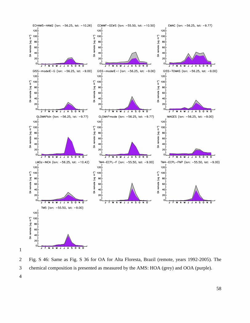
Fig. S 46: Same as Fig. S 36 for OA for Alta Floresta, Brazil (remote, years 1992-2005). The 2

chemical composition is presented as measured by the AMS: HOA (grey) and OOA (purple). 3

4

59

1

Fig. S 47: Same as Fig. S 36 for OA for Melpitz, Germany (remote, years 2008 and 2009). The 2


4

60

1

Fig. S 48: Same as Fig. S 36 for OA for Mace Head, Ireland (remote, years 2002, 2008 and 2009). 2

The chemical composition is presented as measured by the AMS: HOA (grey) and OOA (purple). 3

4

61

1

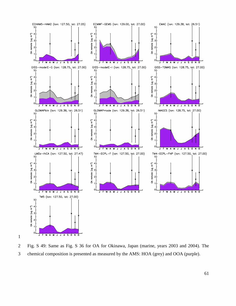
Fig. S 49: Same as Fig. S 36 for OA for Okinawa, Japan (marine, years 2003 and 2004). The 2


Documents

Supplement of The AeroCom evaluation and …€¦ · 2 CMU-VBS calculates that almost all POC has undergone aging, ... 20 CAM4-Oslo has a mPOA source ... are presented in the Supplement