SUPPLEMENT OF CHAPTER III (MAPPING CRITICAL LEVELS F ... · F. Hayes, CEH Bangor Shutterstock, UK Shutterstock, UK. 2 Chapter 3 was prepared under the leadership of the ICP Vegetation

1

SCIENTIFIC BACKGROUND DOCUMENT A

Version October 2018

SUPPLEMENT OF CHAPTER III (MAPPING CRITICAL LEVELS

FOR VEGETATION) OF THE MODELLING AND MAPPING

MANUAL OF THE LRTAP CONVENTION

Chapter 3 of the Modelling and Mapping Manual of the LRTAP Convention describes the

most up-to-date methodology and establishment of critical levels for adverse impacts of air

pollutant (ozone, sulphur dioxide, nitrogen oxides and ammonia) on vegetation. The current

version of Chapter 3 includes updates to critical levels for ozone agreed at the 30th ICP

Vegetation Task Force Meeting, 14-17 February, 2017, Poznan, Poland.

For ozone, further supporting information is provided in this Scientific Background

Document A (SBD-A) regarding the methodologies and critical levels described in Chapter

3. In addition, a Scientific Background Document B (SBD-B) is available, containing DO3SE

model parameterisations for additional species and information on developing areas of

ozone research and the application of methodologies to further develop ozone critical levels.

Chapter 3 and both scientific background documents are available on the ICP Vegetation

website at http://icpvegetation.ceh.ac.uk.

* International Cooperative Programme on Effects of Air Pollution on Natural Vegetation and Crops

F. Hayes, CEH Bangor

Shutterstock, UK

Shutterstock, UK

http://icpvegetation.ceh.ac.uk/

2

Chapter 3 was prepared under the leadership of the ICP Vegetation and led by Gina Mills,

Head of the ICP Vegetation Programme Coordination Centre (PCC), Centre for Ecology &

Hydrology, Bangor, UK.

A list of recent and past contributors to the content of Chapter 3 and SBD-A is provided

below.

Please refer to this document as: ICP Vegetation (2017). Scientific Background Document

A of Chapter 3 of ‘Manual on methodologies and criteria for modelling and mapping critical

loads and levels of air pollution effects, risks and trends’, UNECE Convention on Long-

range Transboundary Air Pollution. Accessed on [date of consultation] at

http://icpvegetation.ceh.ac.uk.

Name Country

Editorial team

Gina Mills UK Lead

Harmens Harmens UK Editor

Håkan Pleijel Sweden Chair Crops Working Group

Patrick Büker UK Chair Forest Trees Working Group

Ignacio González-Fernández Spain Chair (Semi-)natural Vegetation Working Group

Felicity Hayes UK (Semi-)natural Vegetation Working Group

Contributors

Beat Achermann Switzerland Ludger Grünhage Germany

Rocio Alonso Spain Per Erik Karlsson Sweden

Mike Ashmore UK Didier Le Thiec France

Seraina Bassin Switzerland Ian Leith UK

Jürgen Bender Germany Sirkku Manninen Finland

Elke Bergmann Germany Riccardo Marzuoli Italy

Victoria Bermejo Spain Reto Meier Switzerland

Oliver Bethenod France Simone Mereu Italy

Sabine Braun Switzerland Elena Oksanen Finland

Filippo Bussotti Italy Josep Peñuelas Spain

Vicent Calatayud Spain Gunilla Phil-Karlsson Sweden

Esperanza Calvo Spain Martina Pollastrini Italy

Jean-Françoise Castell France Ángela Ribas Spain

Helena Danielsson Sweden Marcus Schaub Switzerland

Susana Elvira Spain David Simpson Sweden

Lisa Emberson UK Juha-Pekka Tuovinen Finland

Angelo Finco Italy Karine Vandermeiren Belgium

Jürg Fuhrer Switzerland Matthias Volk Switzerland

Lina Fusaro Italy Gerhard Wieser Austria

Giacomo Gerosa Italy Matthew Wilkinson UK

Ben Gimeno Spain


3

Table of Contents

1 Introduction ............................................................................................................... 4

2 Method for setting a reference value (Ref10 PODY) for determining flux-based critical levels (Section III.3.1.3 of the manual) ....................................................... 5

2.1 Introduction of the methodology ....................................................................................... 5

2.2 Evaluation of ‘pre-industrial’ O3 ........................................................................................ 5

2.3 Estimated range of O3 concentrations early 1900s.......................................................... 7

2.4 Examples of Ref PODY calculations for different receptors and using constant O3 concentrations in the range of 10 – 25 ppb ..................................................................... 8

2.5 References ....................................................................................................................... 9

3 Modelling the O3 concentration at the top of the canopy (Section III.3.4.2 of the manual) .................................................................................................................... 11

3.1 Introduction .................................................................................................................... 11

3.2 Conversion of O3 concentration at measurement height to canopy height ................... 11

3.3 References ..................................................................................................................... 19

3.4 Appendix ........................................................................................................................ 20

4 Crops – Additional information on O3 flux model parameterisation (Section III.3.5.2 of the manual) ............................................................................................ 24

4.1 Wheat and potato ........................................................................................................... 24

4.2 Tomato ........................................................................................................................... 29

4.3 References ..................................................................................................................... 32

5 Forest trees – Additional information on O3 flux model parameterisation (Section III.3.5.3 of the manual) ............................................................................. 34

5.1 Additional information on parameterisation of forest tree species and sources of information ..................................................................................................................... 34

5.2 Estimating the start (Astart_FD) and end (Aend_FD) of the growing season using the latitude model ............................................................................................................................. 38

5.3 References ..................................................................................................................... 38

6 (Semi-)natural vegetation – Flux model parameterisation for selected (semi-)natural vegetation species and associated flux-effect relationships (Section III.3.5.4.2 of the manual) .......................................................................... 42

6.1 Temperate perennial grasslands ................................................................................... 42

6.2 Mediterranean annual pastures ..................................................................................... 44

6.3 References ..................................................................................................................... 46

7 AOT40-based critical levels and response functions for O3 (Section III.3.7 of the manual) .................................................................................................................... 48

7.1 Introduction .................................................................................................................... 48

7.2 Crops .............................................................................................................................. 48

7.3 Forest trees .................................................................................................................... 52

7.4 (Semi-)natural vegetation ............................................................................................... 55

7.5 References ..................................................................................................................... 58

4

1 Introduction

This Scientific Background Document A (SBD-A) contains supplementary information for Chapter 3 (‘Mapping critical levels for vegetation’) of the Modelling and Mapping Manual of the Convention on Long-range Transboundary Air Pollution (LRTAP), specifically for ozone (O3) critical levels for vegetation. Chapter 3 of the manual was prepared under the leadership of the ICP Vegetation and was fully revised to include updates to critical levels for O3 agreed at the 30th ICP Vegetation Task Force Meeting, 14-17 February, 2017, Poznan, Poland. The revised version of Chapter 3 was published in April 2017 on the ICP Vegetation website (http://icpvegetation.ceh.ac.uk). Where relevant, reference is made within brackets to the appropriate sections of Chapter 3.

SBD-A contains further information on (with reference to relevant Section in the manual):

Method for setting a reference value (Ref10 PODY) for determining flux-based critical levels (Section III.3.1.3);

Modelling the O3 concentration at the top of the canopy (Section III.3.4.2);

Scientific bases of the parameterisation of the O3 flux models used to establish

critical levels for crops (Section III.3.5.2), forest trees (Section III.3.5.3) and (semi-) natural vegetation (Section III.3.5.4);

Scientific bases of O3 concentration-based (AOT40) dose-response relationships

and critical levels for crops, forests trees and (semi-)natural vegetation (Section III.3.7);

O3-sensitivity of plant species.

In the previous version of Chapter 3 of the manual, much of the information related to bullet points two and three was available in the Annexes of Chapter 3.


5

2 Method for setting a reference value (Ref10 PODY) for determining flux-based critical levels (Section III.3.1.3 of the manual)

2.1 Introduction of the methodology

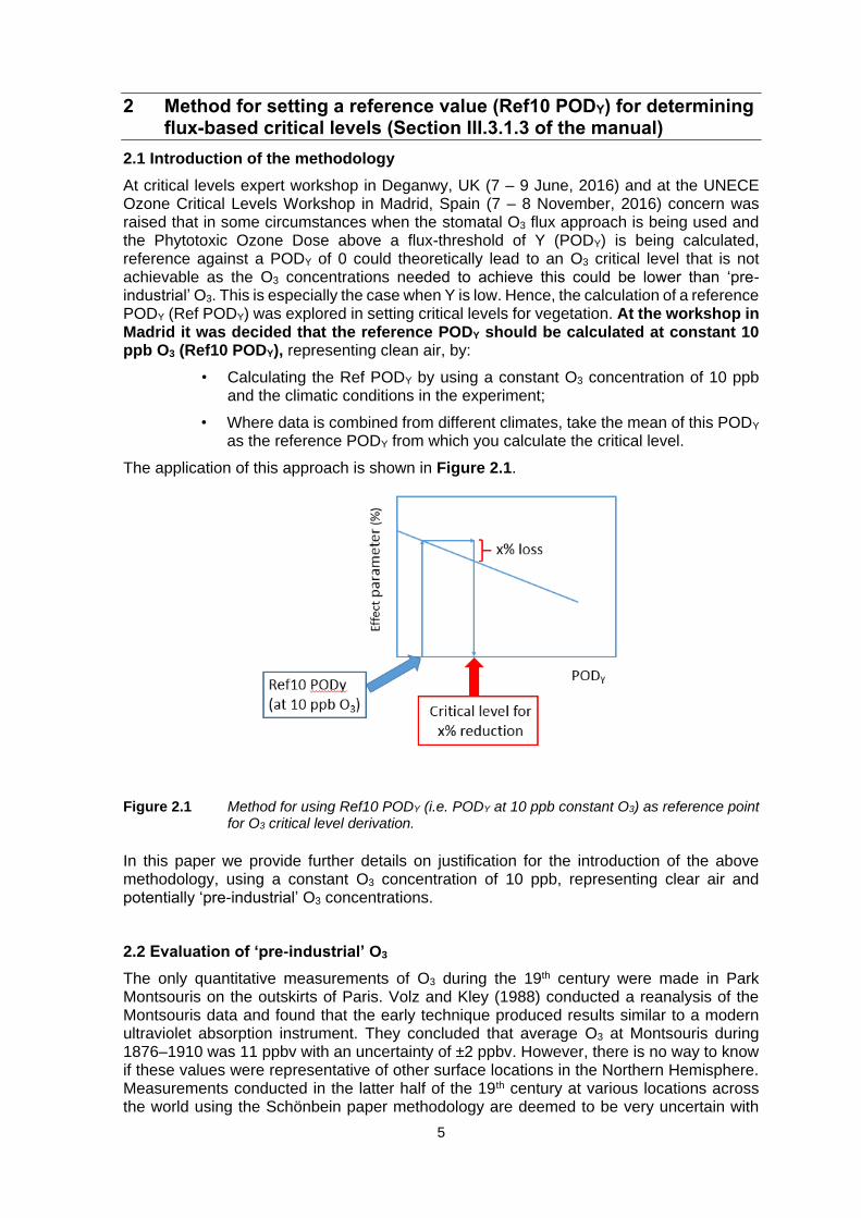
At critical levels expert workshop in Deganwy, UK (7 – 9 June, 2016) and at the UNECE Ozone Critical Levels Workshop in Madrid, Spain (7 – 8 November, 2016) concern was raised that in some circumstances when the stomatal O3 flux approach is being used and the Phytotoxic Ozone Dose above a flux-threshold of Y (PODY) is being calculated, reference against a PODY of 0 could theoretically lead to an O3 critical level that is not achievable as the O3 concentrations needed to achieve this could be lower than ‘pre-industrial’ O3. This is especially the case when Y is low. Hence, the calculation of a reference PODY (Ref PODY) was explored in setting critical levels for vegetation. At the workshop in Madrid it was decided that the reference PODY should be calculated at constant 10 ppb O3 (Ref10 PODY), representing clean air, by:

• Calculating the Ref PODY by using a constant O3 concentration of 10 ppb and the climatic conditions in the experiment;

• Where data is combined from different climates, take the mean of this PODY as the reference PODY from which you calculate the critical level.

The application of this approach is shown in Figure 2.1.

Figure 2.1 Method for using Ref10 PODY (i.e. PODY at 10 ppb constant O3) as reference point for O3 critical level derivation.

In this paper we provide further details on justification for the introduction of the above methodology, using a constant O3 concentration of 10 ppb, representing clear air and potentially ‘pre-industrial’ O3 concentrations.

2.2 Evaluation of ‘pre-industrial’ O3

The only quantitative measurements of O3 during the 19th century were made in Park Montsouris on the outskirts of Paris. Volz and Kley (1988) conducted a reanalysis of the Montsouris data and found that the early technique produced results similar to a modern ultraviolet absorption instrument. They concluded that average O3 at Montsouris during 1876–1910 was 11 ppbv with an uncertainty of ±2 ppbv. However, there is no way to know if these values were representative of other surface locations in the Northern Hemisphere. Measurements conducted in the latter half of the 19th century at various locations across the world using the Schönbein paper methodology are deemed to be very uncertain with

6

respect to absolute O3 values (Cooper et al., 2014). Despite the uncertainty in absolute values, these measurements showed that 1) 19th century seasonal O3 most often peaked in spring, followed by winter; seasonal O3 minima most frequently occurred in summer and autumn, and 2) studies that compared late 19th century estimated O3 to late 20th century ultraviolet absorption O3 measurements generally concluded that average O3 increased by about a factor of two (Cooper et al., 2014) or more (Anfossi et al., 1991; Volz and Kley, 1988) during the 20th century.

Despite the uncertainty of the Schönbein method, there is one set of late 19th century Schönbein measurements that is difficult to dismiss. Measurements made between 1874 and 1909 at Pic du Midi, France, 3000 m above sea level, used the same type of paper and techniques as those employed at Montsouris (Marenco et al., 1994). Accounting for differences in pressure and humidity between Pic du Midi and Montsouris, Marenco et al. (1994) used the Montsouris regression to estimate that Pic du Midi O3 concentrations were approximately 10 ppbv during 1874–1895, with a springtime peak and wintertime minimum. From 1895 until the end of the record in 1909 O3 increased steadily to 14 ppbv, while O3 at Montsouris at this time decreased. Marenco et al. (1994) point out that the increase in O3 at Pic du Midi coincided with global increases in methane concentrations, while the O3 decrease at Montsouris may have been the result of increased emission of NO in Paris that reduced O3 concentrations by titration at nearby Montsouris. While the Pic du Midi O3 mixing ratios appear to be more reliable than any other record outside of Montsouris, the results raise the question why O3 at 3 km above sea level at Pic du Midi, a site representing the free troposphere most of the time, was no greater than O3 at the low elevation site of Montsouris. This lack of a vertical O3 gradient in the lower troposphere is in direct contrast with O3 sonde observations from around the world that showed a consistent increase in O3 with altitude during the 1980s and 1990s (Logan, 1999). The latest generation of atmospheric chemistry models taking part in the Atmospheric Chemistry and Climate Model Intercomparison Project (ACCMIP) show a vertical O3 gradient in the northern mid-latitude lower troposphere during the 1850s that is weaker than the period 1996–2005, but the models overestimate 1850s lower tropospheric O3 by a factor of two compared to Pic du Midi and Montsouris (Stevenson et al., 2013). ACCMIP estimated surface O3 in the northern hemisphere mid-latitudes in 1850 to be more than 40% lower than in 2000, with absolute decreases more than 25 ppbv for the Mediterranean, much of Asia, and the western USA due to less precursor emissions (Young et al., 2013).

Figure 2.2 O3 evolution in the free atmosphere over Western Europe, from measurement at the Pic du Midi and various European stations at high altitudes. Source: Marenco et al. (1994).

7

Marenco et al. (1994) showed an exponential increase in O3 across Western Europe using measurements from several locations, beginning with the Pic du Midi Schönbein measurements in the 1870s followed by short-term quantitative measurements at several high altitude sites in Switzerland, Germany, and France from the 1930s through the early 1990s (Figure 2.2). They concluded that O3 increased by a factor of 5 between the late 1800s and the early 1990s and by a factor of 2 between the 1950s and early 1990s. This increase corresponds to the global increase in fossil fuel combustion summarized by the IPCC Fifth Assessment Report (IPCC, 2013).

2.3 Estimated range of O3 concentrations early 1900s

Table 2.1 provides an estimate of surface O3 concentrations in the Northern Hemisphere based on the concentrations in 2000 for sites at different elevations (Cooper et al., 2014) and assuming a rise in surface O3 concentration of a factor 2 (Cooper et al., 2014), 3 (Marenco et al., 1994) or 5 (Marenco et al., 1994). Equally, the rise in surface O3 concentration by a factor 2 could also reflect the ground-level O3 concentration in the 1950s as O3 concentrations might have doubled since then (Cooper et al., 2014; Marenco et al., 1994). The average surface O3 concentration at low and high elevation sites agrees well with measurements at Montsouris and Pic du Midi (see introduction) when assuming a rise in surface O3 concentration by a factor 3 between 1900 and 2000. The Royal Society (2008) came to the conclusion that a background O3 concentration of 10 – 15 ppbv in 1900 had doubled to 20 – 30 ppbv by 1980 and has since then risen by another 5 ppbv till 2007. The world’s longest continuous O3 record is from the Arkona-Zingst site on the northern German coast. In the late 1950s and early 1960s annual mean O3 concentrations were between 15 – 20 ppbv, which had doubled by the end of the 20th century (Cooper et al., 2014).

Table 2.1 Estimate range of ground-level O3 concentration in 1900 at sites in the Northern Hemisphere, based on the O3 concentration at the sites in 2000 (Cooper et al., 2014), and assuming a linear rise in ground-level O3 concentration by a factor 2, 3 and 5 between 1900 and 2000.

Rise since 1900 Factor 2 Factor 3 Factor 5

Year 2000 1900 1900 1900

Sites Elevation (m) Ozone (ppbv) Ozone (ppbv) Ozone (ppbv) Ozone (ppbv)

Barrow, Alaska 0 27 13 9 5

Arkona-Zingst, Germany 0 28 14 9 6

Storhofdi, Iceland 100 38 19 13 8

Japanese MBL 100 44 22 15 9

Mace Head, Ireland 200 39 19 13 8

US Pacific MBL 200 32 16 11 6

Hohenpeissenberg, Germany 1000 41 21 14 8

Arosa, Switzerland 1800 45 22 15 9

Lassen NP, California, USA 1800 40 20 13 8

Mt Happo, Japan 1900 51 25 17 10

Zugspitze, Germany 3000 53 27 18 11

Summit, Greenland 3200 45 23 15 9

Mauna Loa, Hawaii, USA 3400 40 20 13 8

Jungfraujoch, Switzerland 3600 54 27 18 11

Average All 41 21 14 8

≤200 m 35 17 12 7

≥1000 m 46 23 15 9

8

2.4 Examples of Ref PODY calculations for different receptors and using constant O3 concentrations in the range of 10 – 25 ppb

The DO3SE (Deposition of O3 for Stomatal Exchange) model (https://www.sei-international.org/do3se) was used to calculate stomatal O3 fluxes at a constant O3 concentration of 10, 15, 20 or 25 ppb, applying either the parameterisations as defined in the Modelling and Mapping Manual of the LRTAP Convention (LRTAP Convention, 2017) or local parameterisations where appropriate. Stomatal O3 fluxes, i.e. Phytotoxic Ozone Doses (PODs), were calculated for different vegetation types, based on experiments conducted in various years under varying climatic conditions. For wheat and potato, data used in the establishment of the flux-effect relationships as defined in the Modelling and Mapping Manual were used. For trees, data described by Büker et al. (2015) were used. In addition, PODY was calculated for different plant species for 2010 using climate data from a gradient of seven sites across Europe, i.e. Östad (SE), Cairngorm, Auchencorth, Harwell (all UK), Giessen (DE), Arconate (IT), Tres Cantos (ES). The resulting O3 stomatal fluxes are referred to as reference PODY (Ref PODY). The average reference PODY for the different plant species or plant functional types are shown in Figure 2.3 and 2.4.

As to be expected, Ref PODY is lowest for crops (Ref PODY = 0) as the flux threshold Y is 6 nmol m-2 s-1 and the accumulation period is shorter. Ref PODY is higher when using a generic crop flux model for application in integrated assessment modelling (Crop IAM, based on wheat parameterisation) as Y for this model is 3 nmol m-2 s-1 and the accumulation period is longer (LRTAP Convention, 2017). Compared with crops, Ref PODY is higher for (semi-)natural vegetation and tree species due to the low Y value of 1 nmol m-2 s-1 and the longer accumulation period (LRTAP Convention, 2017). Ref PODY increases linearly with reference O3 concentration (R2 >0.97). Ref PODY is generally lower for needle leaf trees than deciduous broadleaf trees; remarkable are the high Ref PODY values for poplar, more than a factor two higher than for other deciduous broadleaf tree species, primarily due to its higher maximum stomatal conductance.

Figure 2.3. Reference Phytotoxic Ozone Dose (PODY) calculated at a constant O3 concentration ranging from 10 to 25 ppbv for crops and (semi-)natural vegetation. Y = 6, 6, 3 and 1 for wheat, potato, generic crop (Cr.IAM) and Trifolium species (T.sub = Trifolium subterraneum; T.rep. = Trifolium repens) respectively. T.rep. values are an average for seven sites in 2010. Bars show mean + one SD.

0

4

8

12

16

20

Wheat Potato Cr.IAM T.sub. T.rep.

Re

fPO

DY

(m

mo

l m

-2)

Reference ozone (ppbv)

Crops & (semi-)natural

10 ppbv

15 ppbv

20 ppbv

25 ppbv

7 sites, 2010: - tomato = 0 mmol m-2

- wheat & potato: <0.2

https://www.sei-international.org/do3se

https://www.sei-international.org/do3se

9

Figure 2.4 Reference Phytotoxic Ozone Dose (PODY) calculated at a constant O3 concentration ranging from 10 to 25 ppbv for trees; Y = 1 for all tree species. Bars show mean + one SD. Top: Broadleaf deciduous tree species (B.2010 = Beech for seven sites in 2010; Be/Bi = Beech/Birch; T.oak = temperate oak; H.oak = Holm oak; Bl.dec. = all Broadleaved deciduous trees; values for poplar were divided by two. Bottom: Needleleaf tree species; N.spruce = Norway spruce; N.s.2010 = Norway spruce for seven sites in 2010; A.pine = Aleppo pine; S.pine = Scots pine; N.leaf = all needleleaf trees.

2.5 References

Anfossi, D., Sandroni, S, Viarengo, S., 1991. Tropospheric ozone in the nineteenth century: The Moncalieri series. Journal of Geophysical Research 96: 17,349-17,352.

Büker, P., Feng, Z., Uddling, J., Briolat, A., Alonso, R., Braun, S., Elvira, S., Gerosa, G., Karlsson, P.E., Le Thiec, D., Marzuoli, R., Mills, G., Oksanen, E., Wieser, G., Wilkinson, M., Emberson, L.D.. 2015. New flux based dose-response relationships for ozone for European forest tree species. Environmental Pollution 206: 163-174.

Cooper, O R., Parrish, D.D., Ziemke, J., Balashov, N.V., Cupeiro, M., Galbally, I.E., Gilge, S., Horowitz, L., Jensen, N.R., Lamarque, J.F., Naik, V., Oltmans, S.J., Schwab, J., Shindell, D.T., Thompson, A.M., Thouret, V., Wang, Y., Zbinden, R.M., 2014. Global distribution and trends of tropospheric ozone: An observation-based review, Elementa: Science of the Anthropocene 2, 000029, doi:10.12952/journal.elementa.000029.

IPCC (2013) Climate Change 2013 – The Physical Science Basis. Cambridge University Press, Cambridge, UK.

0

4

8

12

16

20

Beech B.2010 Birch Be/Bi T.oak H.oak Poplar Bl.dec.

RefP

OD

1 (m

mo

l m

-2)

Reference ozone (ppbv) (:2)

Broadleaved trees

10 ppbv

15 ppbv

20 ppbv

25 ppbv

0

4

8

12

16

20

N.spruce N.s.2010 A.pine S.pine N.leaf

RefP

OD

1 (m

mo

l m

-2)

Reference ozone (ppbv)

Needleleaf trees

10 ppbv

15 ppbv

20 ppbv

25 ppbv

10

LRTAP Convention, 2017. Manual on Methodologies and Criteria for Modelling and Mapping Critical Loads & Levels and Air Pollution Effects, Risks and Trends. Chapter 3: Mapping Critical Levels for Vegetation (Mills, G., Ed.). http://icpvegetation.ceh.ac.uk/publications/documents/Ch3-MapMan-2016-05-03_vf.pdf

Logan, J.A., 1999. An analysis of ozonesonde data for the troposphere: Recommendations for testing 3-D models and development of a gridded climatology for tropospheric ozone. Journal of Geophysical Research 104: 16,115–16,150.

Marenco, A., Gouget, H., Nédélec, P., Pagés, J-P., 1994. Evidence of a long-term increase in tropospheric ozone from Pic du Midi series: consequences: positive radiative forcing. Journal of Geophysical Research 99: 16,617–16,632.

Royal Society, 2008. Ground-level ozone in the 21st century: future trends, impacts and policy implications. The Royal Society, London, UK.

Stevenson, D.S., Young, P.J., Naik, V., Lamarque, J.-F., Shindell, D.T., Voulgarakis, A., Skeie, R.B., Dalsoren, S.B., Myhre, G., Berntsen, T.K., Folberth, G.A., Rumbold, S.T., Collins, W.J., MacKenzie, I.A., Doherty, R.M., Zeng, G., van Noije, T.P.C., Strunk, A., Bergmann, D., Cameron-Smith, P., Plummer, D.A., Strode, S.A., Horowitz, L., Lee, Y.H., Szopa, S., Sudo, K., Nagashima, T., Josse, B., Cionni, I., Righi, M., Eyring, V., Conley, A., Bowman, K.W., Wild, O., Archibald, A., 2013. Tropospheric ozone changes, radiative forcing and attribution to emissions in the Atmospheric Chemistry and Climate Model Intercomparison Project (ACCMIP). Atmospheric Chemistry and Physics 13: 3063–3085.

Volz, A., Kley, D., 1988. Evaluation of the Montsouris series of ozone measurements made in the 19th century. Nature 332: 240–242.

Young, P.J., Archibald, A.T., Bowman, K.W., Lamarque, J.-F., Naik, V., Stevenson, D.S., Tilmes, S., Voulgarakis, A., Wild, O., Bergmann, D., Cameron-Smith, P., Cionni, I., Collins,W.J., Dalsøren, S.B., Doherty, R.M., Eyring, V., Faluvegi, G., Horowitz, L.W., Josse, B., Lee, Y.H., MacKenzie, I.A., Nagashima, T., Plummer, D.A., Righi, M., Rumbold, S.T., Skeie, R.B., Shindell, D.T., Strode, S.A., Sudo, K., Szopa, S., Zeng, G., 2013. Preindustrial to end 21st century projections of tropospheric ozone from the Atmospheric Chemistry and Climate Model Intercomparison Project (ACCMIP), Atmospheric Chemistry and Physics 13: 2063–2090.

http://icpvegetation.ceh.ac.uk/publications/documents/Ch3-MapMan-2016-05-03_vf.pdf

http://icpvegetation.ceh.ac.uk/publications/documents/Ch3-MapMan-2016-05-03_vf.pdf

11

3 Modelling the O3 concentration at the top of the canopy (Section III.3.4.2 of the manual)

3.1 Introduction

The O3 concentrations needed for the calculation of the POD and the critical levels are the concentrations which occur just at the upper limit of the laminar boundary layer of the receptors’ leaves. Within exposure systems such as open-top chambers, where air flow is omnidirectional, the exposure concentration measured at the top of the canopy reflects the O3 concentration at the upper boundary of the leaves. Under unenclosed field conditions, it was decided that the O3 concentration at the top of the canopy provides a reasonable estimate of the O3 concentration at the upper surface boundary of the laminar boundary layer near the flag leaf (in the case of wheat) and the sunlit upper canopy leaves (in the case of other receptors). Thus, the O3 concentration at the top of the canopy should be available for determining each of the indices used.

Unfortunately O3 concentration is generally not measured at the top of the canopy but well

above it in the case of crops, or well below it in the case of forests (DO3SE, 2014). For

crops and other low vegetation, canopy-top O3 concentrations may be significantly lower

than those at conventional measurement heights of 2-5m above the ground (Figure 3.1a),

and hence use of measured data, directly or after spatial interpolation, may lead to

significant overestimates of O3 concentrations and hence of the degree of exceedance of

critical levels. In contrast, for forests, measured data at 2-5m above the ground may

underestimate O3 concentration at the top of the canopy (Figure 3.1b). The difference in

O3 concentration between measurement height and canopy height is a function of several

factors, including wind speed, atmospheric stability (note how in Figure 3.1 the O3

concentration profile changes with atmospheric stability) and other meteorological factors,

canopy height, surface roughness and the total flux of O3, Ftot.

Conversion of O3 concentration at measurement height to that at canopy-top height (ztgt) can be best achieved with an appropriate deposition model. It should be noted, however, that the flux-gradient relationships these models depend on are not strictly valid within the roughness sublayer (up to 2-3 times canopy height) or in a heterogeneous landscape, so even such detailed calculations can provide only approximate answers. The model chosen will depend upon the amount of meteorological data that is available. 3.2 Conversion of O3 concentration at measurement height to canopy height

Three methods are included here which can be used to achieve the necessary conversion if (a) no meteorological data are available at all, if (b) all the important meteorological measurements are available, or if (c) some basic measurements are available. Method a) Tabulated gradients

If no meteorological data are available at all, then a simple tabulation of vertical O3 gradients can be used. The relationship between O3 concentrations at a number of different heights has been estimated with the EMEP deposition module (Emberson et al., 2000b), using meteorology from about 30 sites across Europe. Data were produced for an arbitrary crop surface and for short grasslands and forest trees (see Table III.7 in Modelling and Mapping Manual). For the crop surface, the assumptions made here are that we have a 1 m high crop with gmax = 450 mmol O3 m-2 PLA s-1. The total leaf surface area index (LAI) is set to 5 m2 PLA m-2, and the green LAI is set at 3 m2 PLA m-2, assumed to give a canopy-scale phenology factor (fphen) of 0.6. The soil moisture factor (fSW) is set to 1.0. Constant values of these parameters are used throughout the year in order to avoid problems with trying to estimate growth stage in different areas of Europe. The concentration gradients thus derived are most appropriate to a fully developed crop but will serve as a reasonable

12

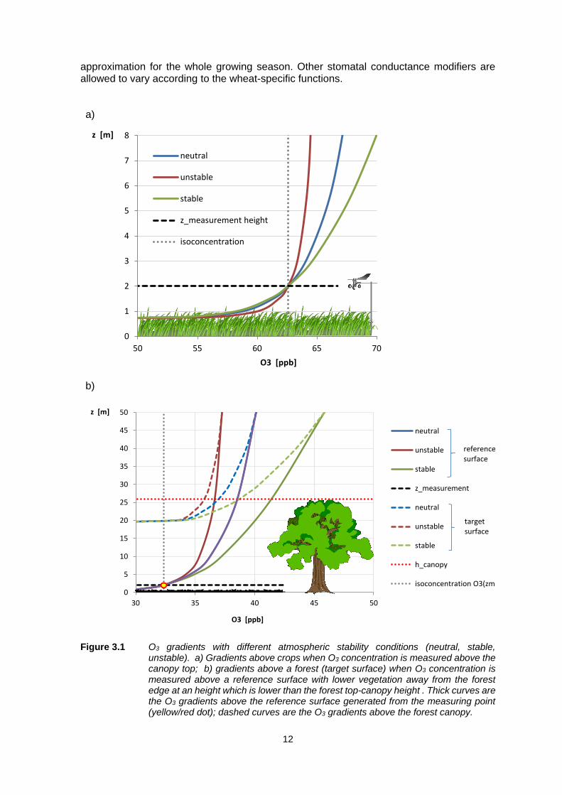
approximation for the whole growing season. Other stomatal conductance modifiers are allowed to vary according to the wheat-specific functions. a)

b)

Figure 3.1 O3 gradients with different atmospheric stability conditions (neutral, stable,

unstable). a) Gradients above crops when O3 concentration is measured above the canopy top; b) gradients above a forest (target surface) when O3 concentration is measured above a reference surface with lower vegetation away from the forest edge at an height which is lower than the forest top-canopy height . Thick curves are the O3 gradients above the reference surface generated from the measuring point (yellow/red dot); dashed curves are the O3 gradients above the forest canopy.

0

1

2

3

4

5

6

7

8

50 55 60 65 70

z [m]

O3 [ppb]

neutral

unstable

stable

z_measurement height

isoconcentration

0

5

10

15

20

25

30

35

40

45

50

30 35 40 45 50

z [m]

O3 [ppb]

neutral

unstable

stable

z_measurement

neutral

unstable

stable

h_canopy

isoconcentration O3(zm)

reference surface

target surface

13

For short grasslands, canopy height was set to 0.1 m, gmax to 270 mmol O3 m-2 PLA s-1 and fSWP set to 1.0. All other factors are as given for grasslands in Emberson et al. (2000b). For the micrometeorology, the displacement height (d) and roughness length (z0) are set to 0.7 and 0.1 of canopy height (z1), respectively. Table III.7 in the Modelling and Mapping Manual shows the average relationship between O3 concentrations at selected heights, derived from runs of the EMEP module over May-July, and selecting the noontime factors as representative of daytime multipliers. O3 concentrations are normalised by setting the 20 m value to 1.0.

To use Table III.7, O3 concentration measurements made above crops or grasslands may simply be extrapolated downwards to the canopy top for the respective vegetation. For example, with 30 ppb measured at 3 m height (above ground level) in a crop field, the

concentration at 1 m would be 30.0 ppb (0.88/0.95) = 27.8 ppb. For short grasslands we

would obtain 30.0 ppb (0.74/0.96) = 23.1 ppb at canopy height 0.1 m. Experiments have shown that the vertical gradients found above for crops also apply well to tall (0.5m) grasslands. Some judgement may then be required to choose values appropriate to different vegetation types.

For forests, O3 concentrations must often be derived from measurements made over grassy areas or other land cover types. In principle, the O3 concentration measured over land-use X (e.g. short grasslands) could be used to estimate the O3 concentration at a reference height, and then the gradient profile appropriate for desired land use Y could be applied. However, in order to keep this simple methodology manageable, and in view of the uncertainties inherent in making use of any profile near the canopy itself, it is suggested that concentrations are estimated by extrapolating the profiles given in Table III.7 upwards to the canopy height for forests. As an example, if we measure 30 ppb at 3 m above short grassland, the concentration at 20 m is estimated to be 30.0 ppb x (1.0/0.96) = 31.3 ppb.

It should be noted that the profiles shown in Table III.7 are representative only, and that site-specific calculations would provide somewhat different numbers. However, without local meteorology and the use of a deposition model, the suggested procedure should give an acceptable level of accuracy for most purposes. Gerosa et al. (2017.) verified that the tabulated gradients allowed them to calculate O3 deposition fluxes for a mature forest that were in very good agreement with those directly measured with the eddy covariance technique. Method b) Concentration profiles with stability effects

If all the important meteorological measurements are available, two possible cases can be envisaged: (1) if all the measurements were done above the desired (target) vegetation canopy or (2) if the measurements were done above a vegetated surface which is different from the desired surface.

Case 1: O3 and meteorological measurements available above the target canopy

If the wind speed and the O3 concentration were measured above the vegetation canopy, respectively at height zm,w and height zm,O3, the O3 concentration at the top of the canopy (the target height ztgt) can be obtained by making use of the big-leaf approximation and of the constant-flux assumption in the definition of the aerodynamic resistance. In the following, the roughness sub-layer affecting the concentration profiles near the canopy top has been neglected. A simple method for correcting for the roughness sub-layer can be found in Tuovinen and Simpson (2008). With the geometry illustrated in Figure 3.2, the O3 concentration at the top of the canopy O3(ztgt) can be calculated with the following equation:

14

(1) 𝑂3(𝑧𝑡𝑔𝑡) = 𝑂3(𝑧𝑚,𝑂3) ∙ [1 −𝑅𝑎(𝑧𝑡𝑔𝑡 , 𝑧𝑚,𝑂3)

𝑅𝑎(𝑑 + 𝑧0, 𝑧𝑚,𝑂3) + 𝑅𝑏 + 𝑅𝑠𝑢𝑟𝑓]

where O3(zm,O3) is the available O3 measurement above the canopy, Ra(ztgt, zm,O3) is the

aerodynamic resistance between the height where O3 was measured and the top canopy height (the target height), Ra(d + z0, zm,O3) is the aerodynamic resistance to O3 deposition,

i.e. the atmospheric resistance between the height where O3 was measured and the height of the upper boundary of the laminar sub-layer of the theoretical big-leaf surface, Rb is the resistance to O3 diffusion in the laminar sub-layer, and Rsurf is the overall resistance to O3 deposition to the underlying surfaces. The latter includes the stomatal resistance to O3 uptake Rstom, the resistance of the external cuticles Rext, the soil resistance to O3 deposition Rsoil and the air resistance to O3 transfer within the vegetation layer Rinc.

Figure 3.2 Resistive network for the calculation of the top-canopy O3 concentration when O3

and meteorological measurements are available ABOVE the vegetated surface (Case 1).

The calculation of the aerodynamic resistance Ra requires the estimation of the friction velocity u* above the vegetated surface by the following equation

(2) 𝑢∗ =

𝑘 ∙ 𝑢(𝑧𝑚,𝑤)

ln (𝑧𝑚,𝑤 − 𝑑

𝑧0) − 𝛹𝑀 (

𝑧𝑚,𝑤 − 𝑑𝐿

) + 𝛹𝑀 (𝑧0𝐿)

where k is the von Kármán constant (0.41), u(zm,w) is the wind speed measured at the

height zm,w, d is the displacement height usually assumed as 2/3 of the canopy height, z0 is the roughness length usually assumed as 1/10 of the canopy height, and ΨM(. . ) is the

z

zm,w

d

d+z0

zm,O3

GG,2016

Ra(d+z0, zm,O3)

O3(zm,O3)

Rinc

Rstom

Rext

Rsoil

Rb

O3(ztgt)

Ra(ztgt, zm,O3)

15

integral form of the similarity function for momentum which takes into account the stability of the atmospheric surface layer in terms of the Obukhov length L (1/L = 0 if the atmosphere is neutral, 1/L < 0 if the atmosphere is unstable, 1/L > 0 if the atmosphere is stable) (Garratt, 1992).

With (adimensional length) as the argument, the function ΨM() is defined as (Dyer, 1974; Garratt, 1992):

(3) 𝑀() = {ln [

1 + 𝑥2

2∙ (1 + 𝑥

2)2

] − 2 arctan(𝑥) +𝜋

2, 𝑤ℎ𝑒𝑛 < 0

− 5, 𝑤ℎ𝑒𝑛 ≥ 0

with 𝑥 = (1 − 16 ∙ )1 4⁄ . Once u* is known, the two Ra resistances in (1) can be calculated as follows:

(4)

𝑅𝑎(𝑧𝑡𝑔𝑡 , 𝑧𝑚,𝑂3) =1

𝑘 ∙ 𝑢∗[ln (

𝑧𝑚,𝑂3 − 𝑑

𝑧𝑡𝑔𝑡 − 𝑑) − 𝛹𝐻 (


𝐿)

+ 𝛹𝐻 (𝑧𝑡𝑔𝑡 − 𝑑

𝐿) ]

(5) 𝑅𝑎(𝑑 + 𝑧0, 𝑧𝑚,𝑂3) =1

𝑘 ∙ 𝑢∗[ln (


𝑧0) − 𝛹𝐻 (


𝐿) + 𝛹𝐻 (

𝑧0𝐿) ]

with ΨH(. . ), the similarity function for heat, defined as (Dyer, 1974; Garratt, 1992):

(6) 𝐻() = {2 𝑙𝑛 [

1 + 𝑥2

2] , 𝑤ℎ𝑒𝑛 < 0

− 5, 𝑤ℎ𝑒𝑛 ≥ 0

with 𝑥 = (1 − 16 ∙ )1 4⁄ . The Obukhov length needed to account for the atmospheric stability can be estimated by following the procedure illustrated in the appendix of this chapter, or a guess value can be assumed according to the typical conditions of the area for which the fluxes should be calculated (e.g. 1/L=0 for neutral conditions, 1/L=-0.01 for unstable or 1/L=-0.1 for very unstable conditions, 1/L=+0.01 for stable conditions). If no information on atmospheric stability is known at all, the ΨM(. . ) and ΨH(. . ) functions in (1), (4) and (5) can be set to zero and then the atmosphere is assumed as neutral.

The resistance to O3 diffusion in the laminar sub-layer Rb can be calculated with the formulation of Wesely and Hicks (1977):

(7) 𝑅𝑏 =2

𝑘 ∙ 𝑢∗(𝑆𝑐

𝑃𝑟)2/3

where k is the von Kármán constant, Sc=0.93 is the Schmidt number for O3, and Pr=0.71 is the Prandtl number of air.

The surface resistance to O3 deposition Rsurf is defined as follows:

(8) 𝑅𝑠𝑢𝑟𝑓 =

1

𝐿𝐴𝐼𝑅𝑠𝑡𝑜

+𝑆𝐴𝐼𝑅𝑒𝑥𝑡

+1

𝑅𝑖𝑛𝑐 + 𝑅𝑠𝑜𝑖𝑙

16

where Rsto is the leaf-scale stomatal resistance to O3 of the vegetated surface, Rext is the leaf-scale resistance of the external vegetation surfaces (e.g. cuticles, bark, etc.) to O3 deposition, Rsoil is the soil resistance to O3 deposition, Rinc is the in-canopy air resistance to the O3 transfer to the soil, LAI is the projected leaf area (m2 m-2), and SAI is the surface area of the canopy (green LAI + senescent LAI + twig and branch surfaces). Rsto is a plant species specific function of air temperature and humidity, solar radiation and soil water content. It can be modelled – as described in the manual – by means of the Jarvis–Stewart algorithm (Jarvis, 1976; Emberson et al., 2000a) and data on the photosynthetically active radiation (light), air temperature (temp) and relative humidity (to calculate vapour pressure deficit - VPD) at the canopy top (Tuovinen and Simpson, 2008), the soil water potential (SW), and plant phenology (phen):

(9)

𝑅𝑠𝑡𝑜 =1

𝑔𝑠𝑡𝑜

=1

𝑔𝑚𝑎𝑥 ∙ [min (𝑓𝑝ℎ𝑒𝑛, 𝑓𝑂3)] ∙ 𝑓𝑙𝑖𝑔ℎ𝑡 ∙ max { 𝑓𝑚𝑖𝑛, (𝑓𝑡𝑒𝑚𝑝 ∙ 𝑓𝑉𝑃𝐷 ∙ 𝑓𝑆𝑊)}

where gmax is the stomatal conductance of O3 in non-limiting conditions and the f functions fphen, flight, ftemp, fVPD, fSW are species-specific functions which describe the variation of

the stomatal conductance with phenology, light, air temperature, leaf-to-air vapour pressure deficit and soil water potential, respectively. For details, see Section III.3.4.3 of the manual on the modelling of the stomatal conductance.

The resistance to cuticular deposition of O3, Rext, and the soil resistance, Rsoil, are set respectively to 2500 s m-1 and 200 s m-1 for consistency with the EMEP model (Simpson et al., 2012).

The in-canopy resistance Rinc can be calculated according to van Pul & Jacobs (1994): (10) 𝑅𝑖𝑛𝑐 = 𝑏 ∙ 𝑆𝐴𝐼 ∙ ℎ/𝑢

∗

where b = 14 m-1 is an empirical constant, h is the height of the canopy and SAI is the surface area of the canopy.

It is worth noticing that all the resistances in the above equations are expressed in the unit of s m-1. Thus, the stomatal conductance, usually given in mmol m-2 s-1, should be converted to m s-1. The conversion can be done by multiplying gsto by R ∙ T/P with the gas constant R = 8.314 J mol-1 K-1, the air temperature T in Kelvin and the atmospheric pressure P in Pa. It should be noted that gstom is the stomatal conductance to O3, and not to water vapour; stomatal conductance to water vapour can be converted to O3 by multiplying it by 0.663. Case 2: Calculation of the O3 concentration over a target surface from measurements made above a different surface

This case typically occurs with forests, for which O3 concentrations must be derived from measurements made over grassy areas or other land-cover types (Gerosa et al., 2017; Tuovinen et al., 2009). The O3 concentrations measured over e.g. short grasslands are used to estimate the O3 concentrations at a reference height that is greater than the forest height, and then the gradient profile appropriate for the forest surface is applied to derive the concentrations at the top of the forest canopy. It should be noted, however, that there are potentially significant uncertainties involved in this approach. In addition to the roughness sub-layer effect mentioned above (Tuovinen & Simpson, 2008), the application of the profile functions presented here inherently assume extensive homogeneous surfaces (i.e. an adequate fetch). The validity of the method is compromised if the measurements are taken close to the forest edge, see for example Tuovinen et al. (2009).

17

The typical situation is that described in Figure 3.3, where the O3 concentration O3(zm,O3) and the wind speed u(zm,O3) are measured over a reference surface (e.g. grassland) at a measuring height zm,O3 and zm,O3 respectively. The aerodynamic features of the reference surface (h, d, z0, LAI, SAI) as well as all the resistances to O3 deposition (ra, rb, rstom, rext, rinc, rsoil) over the reference surface should be known. The same is true for the target surface (e.g. forest), for which h, d, z0, LAI, SAI, as well as all the resistances to O3 deposition (Ra, Rb, Rstom, Rext, Rinc, Rsoil) should be known.

Figure 3.3 Resistive network for the calculation of the O3 concentration at the top of a

target canopy (e.g. forest) when O3 and meteorological measurements are available above a different vegetated surface (e.g. grassland) (Case 2).

The estimation of the O3 concentration at the top of the target canopy O3(ztgt) requires two steps:

i) the calculation of the O3 concentration at an height (above the reference and the target surfaces) where it is not influenced by variations in the underlying surface;

ii) the calculation of the O3 concentration at the desired height above the target surface.

Step i) Calculation of the O3 concentration at a height where it is not influenced by surface variability: First of all the O3 concentration should be calculated at a height zup at which it is not influenced by variation in the properties of the underlying surface. This height is usually assumed at 50 m (Simpson et al., 2012). For this sake the friction velocity u* above the reference surface should be calculated analogous to (2):

(11) 𝑢𝑟𝑒𝑓∗ =

𝑘 ∙ 𝑢(𝑧𝑚,𝑤)

ln (𝑧𝑚,𝑤 − 𝑑𝑟𝑒𝑓𝑧0,𝑟𝑒𝑓

) − 𝛹𝑀 (𝑧𝑚,𝑤 − 𝑑𝑟𝑒𝑓

𝐿) + 𝛹𝑀 (

𝑧0,𝑟𝑒𝑓𝐿

)

z

zup

dd+z0

d

d+z0

GG 2016

Target surfaceReference surface

rb

rstomrext

rinc

rsoil

zm,O3

zm,wr a(

z up, d

+z0)

r a(z m

,O3, z

up)

RstomRext

Rinc

Rsoil

Rb

ztgt

Ra(d+z0, zup) Ra(ztgt, zup)

O3(zm,O3)

O3(ztgt)

O3(zup)

18

where the subscripts ref indicate that the parameters refer to the reference surface (e.g. grassland). The Obukhov length and the ΨM(. . ) function have been already introduced in the previous section.

Then the O3 concentration at the height zup is given by:

(12) 𝑂3(𝑧𝑢𝑝) =

𝑂3(𝑧𝑚,𝑂3)

1 −𝑟𝑎(𝑧𝑚,𝑂3, 𝑧𝑢𝑝)

𝑟𝑎(𝑑𝑟𝑒𝑓 + 𝑧0, 𝑧𝑢𝑝) + 𝑟𝑏 + 𝑟𝑠𝑢𝑟𝑓

where the two atmospheric resistances are given by the following expressions:

(13)

𝒓𝑎(𝑧𝑚,𝑂3, 𝑧𝑢𝑝) =1

𝑘 ∙ 𝑢𝑟𝑒𝑓∗ [ln (

𝑧𝑢𝑝 − 𝑑𝑟𝑒𝑓

𝑧𝑚,𝑂3 − 𝑑𝑟𝑒𝑓) − 𝛹𝐻 (


𝐿)

+ 𝛹𝐻 (𝑧𝑚,𝑂3 − 𝑑𝑟𝑒𝑓

𝐿) ]

(14)

𝒓𝑎( 𝑑𝑟𝑒𝑓 + 𝑧0, 𝑧𝑢𝑝)

=1

𝑘 ∙ 𝑢𝑟𝑒𝑓∗ [ln (


𝑧0,𝑟𝑒𝑓) − 𝛹𝐻 (


𝐿) + 𝛹𝐻 (

𝑧0,𝑟𝑒𝑓

𝐿) ]

with the friction velocity uref

∗ calculated with (11) and the similarity function ΨH(. . ) defined

as in (6). The resistance rb is calculated with (7) by using uref∗ for u∗ . The resistance rsurf is

calculated in a way analogous to what was explained for the case 1 ((8), (9) and (10)) by taking into account the appropriate geometry, LAI, SAI and the f functions for the reference canopy, and by setting rext and rsoil to the values indicated for Rext and Rsoil above. Step ii) Calculation of the O3 concentration at the desired height above the target surface: Once the O3 concentration at the height zup is known, the O3 concentration at the target height canopy 𝑂3(𝑧𝑡𝑔𝑡) above the target surface can be calculated.

First the friction velocity above the target surface u*tgt should be calculated as:

(15) 𝑢𝑡𝑔𝑡∗ =

𝑘 ∙ 𝑢(𝑧𝑢𝑝)

ln (𝑧𝑢𝑝 − 𝑑𝑡𝑔𝑡𝑧0,𝑡𝑔𝑡

) − 𝛹𝑀 (𝑧𝑢𝑝 − 𝑑𝑡𝑔𝑡

𝐿) + 𝛹𝑀 (

𝑧0,𝑡𝑔𝑡𝐿

)

where d and z0 now refer to the target surface (‘tgt’ suffix). The wind speed at the height zup which appears in (15) as u(zup) – the height at which the wind is assumed not to be

influenced by variations in the underlying surface – can be calculated by the following formula:

Equation (16) 𝑢(𝑧𝑢𝑝) =𝑢𝑟𝑒𝑓∗

𝑘∙ [ln (


𝑧0,𝑟𝑒𝑓) − 𝛹𝑀 (


𝐿) + 𝛹𝑀 (

𝑧0,𝑟𝑒𝑓

𝐿)]

where here d and z0 refer to the reference surface (i.e. the grassland).

Then the O3 concentration at the desired height ztgt above the target surface is given by:

(17) 𝑂3(𝑧𝑡𝑔𝑡) = 𝑂3(𝑧𝑢𝑝) ∙ [1 −𝑅𝑎(𝑧𝑡𝑔𝑡 , 𝑧𝑢𝑝)

𝑅𝑎(𝑑 + 𝑧0, 𝑧𝑢𝑝) + 𝑅𝑏 + 𝑅𝑠𝑢𝑟𝑓]

19

where O3(zup) was calculated with (12) and the two atmospheric resistances – which refer

to the target surface – are given by the following expressions:

(18)

𝑅𝑎(𝑧𝑡𝑔𝑡 , 𝑧𝑢𝑝) =1

𝑘 ∙ 𝑢𝑡𝑔𝑡∗ [ln (

𝑧𝑢𝑝 − 𝑑𝑡𝑔𝑡

𝑧𝑡𝑔𝑡 − 𝑑𝑡𝑔𝑡) − 𝛹𝐻 (


𝐿)

+ 𝛹𝐻 (𝑧𝑡𝑔𝑡 − 𝑑𝑡𝑔𝑡

𝐿) ]

(19) 𝑅𝑎(𝑑 + 𝑧0, 𝑧𝑢𝑝) =1

𝑘 ∙ 𝑢𝑡𝑔𝑡∗ [ln (


𝑧0,𝑡𝑔𝑡) − 𝛹𝐻 (


𝐿) + 𝛹𝐻 (

𝑧0,𝑡𝑔𝑡

𝐿) ]

with the friction velocity utgt

∗ calculated with (15) and the similarity function ΨH(. . ) defined

as in (6.The resistance Rb is calculated with (7) by using utgt∗ for u∗ .The resistance Rsurf is

calculated in a way analogous to what was explained for Case 1 ((8), (9) and (10)) by taking into account the appropriate geometry, LAI, SAI and the f functions for the target canopy. A comparison among the O3 concentrations measured at the top of the forest and those estimated at the same level with this methodology, by using measurements taken on a nearby grassland, can be found in Gerosa et al. (2017). The paper discusses also the uncertainties related to different calculation options and their consequences on the estimated POD1SPEC in comparison to the ozone fluxes measured by eddy covariance at the same site.

Method c) Concentration profiles with no stability correction

If no information on atmospheric stability is available, method b) can be simplified by ignoring the stability correction by setting the value of ΨM(. . ) and ΨH(. . ) functions in (1), (4) and (5) (the shaded terms) to zero. By doing so, the atmospheric stability is assumed to be neutral. 3.3 References

DO3SE v.3, 2014. User manual, available at www.sei-international.org/do3se

Dyer, A.J., 1974. A review of flux-profile relationships. Boundary-Layer Meteorology 7: 363–372

Emberson L.D., Ashmore M.R., Cambridge H.M., Simpson D., Tuovinen J.-P., 2000a. Modelling stomatal ozone flux across Europe. Environmental Pollution 109: 403-413.

Emberson, L.D., Simpson, D., Tuovinen, J.-P., Ashmore, M.R., Cambridge, H.M., 2000b. Towards a model of ozone deposition and stomatal uptake over Europe. Norwegian Meteorological Institute, Oslo. EMEP MSC-W Note 6/2000, 57pp.

Garratt, J. R., 1992. The atmospheric boundary layer. Cambridge University Press, Cambridge, UK, 316 pp.

Gerosa, G.A., Marzuoli, R., Monteleone, B., Chiesa, M., Finco, A., 2017. Vertical ozone gradients above forests. Comparison of different calculation options with direct ozone measurements above a mature forest and consequences for ozone risk assessment. Forests 8: 337.

Jarvis P.G., 1976. The interpretation of the variations in leaf water potential and stomatal conductance found in canopies in the field. Philosophical Transactions of the Royal Society of London B – Biological Sciences 273: 593–610.

Simpson, D., Benedictow, A., Berge, H., Bergström, R., Emberson, L.D., Fagerli, H., Flechard, C.R., Hayman, G.D., Gauss, M., Jonson, J.E., Jenkin, M.E., Nýıri, A., Richter, C., Semeena, V.S., Tsyro, S.,

http://www.sei-international.org/do3se

20

Tuovinen, J.-P., Valdebenito, Á., Wind, P., 2012. The EMEP MSC-W chemical transport model – technical description. Atmospheric Chemistry and Physics 12: 7825-7865.

Tuovinen J.-P., Emberson L., Simpson D., 2009. Modelling ozone fluxes to forests for risk assessment: status and prospects. Annals of Forest Science 66: 401.

Tuovinen, J.-P. & Simpson, D., 2008. An aerodynamic correction for the European ozone risk assessment methodology, Atmospheric Environment 42: 8371-8381.

Van Pul W. A. J., Jacobs A. F. G., 1994. The conductance of a maize crop and the underlying soil to ozone under various environmental conditions. Boundary-Layer Meteorology 69: 83-99.

Wesely, M. L. & Hicks, B. B., 1977. Some factors that affect the deposition rates of sulfur dioxide and similar gases on vegetation. Journal of the Air Pollution Control Association 27: 1110-1116.

3.4 Appendix

Estimation of the Obukhov length (L)

The Obukhov length L (m) is an indicator of the atmospheric stability, but its calculation

requires that some other parameters are estimated aside. L is defined by the following

equation:

(20)

𝐿 = −𝑢∗3

𝑘 𝑔𝑇𝐻𝜌 𝑐𝑝

where u* is the friction velocity (m/s), k is the Von Kármán constant (0.41, adim), g is the

gravity acceleration (9.8 m s-2), T is the air temperature (K), H is the sensible heat flux (W

m-2), is the air density (kg m-3), cp is the specific heat at constant pressure (1048 J kg-1 K-

1). Not all these data are usually available from traditional slow meteorological stations, in

particular u* and H. Relatively easy measurements of u* and H can be performed with an

ultrasonic anemometer but nearly always it is not available. Hence, to estimate L a model

of H and u*, and also of the net radiation (Rn) which is required for the H estimation, are

needed.

Estimation of the net radiation (Rn)

Net radiation can be estimated using the methodology proposed by Holtslag & Van Ulden

(1983):

(21)

𝑅𝑛 =

((1 − 𝐴)𝑄𝑠𝑤 + 𝑐1𝑇6 − 𝜎𝑇4 + 𝑐2𝑁)

1 + 𝑐3

where A is the albedo (fraction between 0..1), T is the air temperature K), N is the cloud

cover (%), c1 and c2 are constants (whose values are respectively 5.3110-13 W m-2 and 60

W m-2), is the Stefan-Boltzmann constant (5.67E-08 W m-2 K-4 ), QSW is the shortwave

radiation (the global radiation which is typically available from traditional meteorological

stations, W m-2) and c3 is a temperature dependent parameter which will be presented few

lines below.

The cloud cover N can be estimated from the measured shortwave radiation taking into

account the solar elevation angle (, degree) with the following equation taken from Holtslag

& Van Ulden (1983):

21

(22)

𝑁 = √

1

𝑏1(1 −

𝑄𝑆𝑊(990 𝑠𝑖𝑛 𝜈 − 30)

)𝑏2

where: b1 and b2 are empirical constants whose values are respectively 0.75 and 3.4. The

solar elevation angle ν (degrees) can be calculated by downloading the tool available in the

NOAAweb site (http://www.esrl.noaa.gov/gmd/grad/solcalc/calcdetails.html). The c3

parameter is obtained by the following equation:

(23) 𝑐3 = 0.38 ∙ ((1 − 𝛼) ∙ 𝑆 + 1)/(𝑆 + 1)

where is the water availability parameter described in Beljaars and Holtslag (1989

and1991) and whose values can be taken from Table A3.1 (Hanna & Chang, 1992), and S

is a temperature dependent parameter described by the following equation derived from the

tabulated values of Hanna & Chang (1992):

(24) 𝑆 = 1.5 ∙ 𝑒−0.060208041∙𝑇

with T the air temperature in Celsius degrees.

Table A3.1 Values for the parameter α proposed by Hanna & Chang (1992).

Values for the parameter α

From To Description

0 0.2 Arid desert without rainfalls for months

0.2 0.4 Rural arid area

0.4 0.6 Agricultural fields in periods with no rainfalls for long periods

0.5 1 Urban environment

0.8 1.2 Agricultural fields or forests with sufficient water availability

1.2 1.4 Big lake or ocean, far at least 10 km from the shore

Estimation of the sensible heat flux (H)

Sensible heat fluxes can be modelled using the methodology proposed by Holtslag & Van

Ulden (1983):

(25) 𝐻 =(1 − 𝛼) + 𝑆

1 + 𝑆(𝑅𝑛 + 𝑄𝐴 − 𝐺) − 𝛼𝛽

where QA is the anthropogenic heat flux (which is always set equal to zero as suggested by

Hanna & Chang, 1992), S and are respectively the temperature dependent parameter

and the water availability parameter just described above ((24) and Table A3.1), is a

constant value equal to 20 W m-² which takes into account that sensible heat flux is usually

negative just before the sunset (Hanna & Chang 1992), and G is the ground heat flux

assumed as a fraction of the net radiation

(26) 𝐺 = 𝑎 ∙ 𝑅𝑛

http://www.esrl.noaa.gov/gmd/grad/solcalc/calcdetails.html

22

with a a constant value (a=0.1 for rural areas and a=0.3 for urban areas) taken from Doll

et al. (1985).During the nighttime hours (Rn<50 W m-²) the sensible heat flux is calculated

as H = -β.

Estimation of the friction velocity (u*)

The friction velocity can be estimated following the methodology proposed in Bassin et al. (2003). When H< 1 W m-² (Stable atmosphere) u* is calculated by the following equation:

(27) 𝑢∗ =0.5 𝑘 ∙ 𝑈

𝑙𝑛 ((𝑧𝑟𝑒𝑓 − 𝑑) 𝑧0)⁄(1 + √1 −

4(5 ∙ 𝑔 ∙ 𝑧𝑟𝑒𝑓 ∙ 𝜃∗ ∙ 𝑙𝑛 ((𝑧𝑟𝑒𝑓 − 𝑑) 𝑧0)⁄

𝑘 ∙ 𝑇0 ∙ 𝑈²)

where k is the Von Kármán constant, U is the horizontal wind speed (m s-1), zref is the

measurement height of the wind speed (m), d is the displacement height (m) usually taken

as 2/3 of the canopy height, T0 are the Kelvin degrees at 0°C (i.e. T0=273.15 K), z0 is the

roughness length (m) (z0 values can be taken from the table at page 1.5-12 of WMO, 2008),

g is the gravity acceleration (m s-2) and * is the scale temperature (K) calculated according

to the following equation:

(28) 𝜃∗ =−𝐻

𝜌 ∙ 𝑐𝑝 ∙ 𝑢𝑛𝑒𝑢𝑡𝑟𝑎𝑙∗

where 𝒖𝒏𝒆𝒖𝒕𝒓𝒂𝒍∗ (m s-1) with the following equation:

(29) 𝑢𝑛𝑒𝑢𝑡𝑟𝑎𝑙∗ =

𝑈

𝑘 ln((𝑧𝑟𝑒𝑓 − 𝑑) 𝑧0)⁄

When H> 1 W m-² (unstable atmosphere, the friction velocity is calculated by the following

equation:

(30) 𝑢∗ =𝑘 𝑈

𝑙𝑛 [(𝑧𝑟𝑒𝑓 − 𝑑) 𝑧0]⁄[1 + 𝑑1 𝑙𝑛(1 + 𝑑2𝑑3)]

where d1, d2 and d3 are respectively:

(31) 𝑑1 =

{

0.128 + 0.005 𝑙𝑛 [

𝑧0

(𝑧𝑟𝑒𝑓 − 𝑑)] 𝑖𝑓

𝑧0𝑧𝑟𝑒𝑓 − 𝑑

≤ 0.01

0.107 𝑖𝑓 𝑧0

𝑧𝑟𝑒𝑓 − 𝑑> 0.01

(32) 𝑑2 = 1.95 + 32.6 (𝑧0

𝑧𝑟𝑒𝑓 − 𝑑)

0.45

(33) 𝑑3 =𝐻

𝜌𝑐𝑝

𝑘𝑔(𝑧𝑟𝑒𝑓 − 𝑑)

𝑇0(𝑙𝑛 ((𝑧𝑟𝑒𝑓 − 𝑑) 𝑧0)⁄

𝑘 𝑈)

3

23

References

Holtslag A A, Van Ulden A P., 1983. A simple scheme for daytime estimates of the surface fluxes from routine weather data. Journal of Applied Meteorology and Climatology 22, 517-529

Hanna S R, Chang J C., 1992. Boundary layer parametrizations for applied dispersion modeling over urban areas. Boundary-Layer Meteorology 58, 229-259

NOAA, US Department of Commerce: National Oceanic and Atmospheric Administration. Solar Calculation Details. [Online] http://www.esrl.noaa.gov/gmd/grad/solcalc/calcdetails.html .

Doll D, Ching J K S, Kaneshire J., 1985. Parametrization of subsurfaces heating for soil and concrete using new radiation data. Boundary-Layer Meteorology 32, 351-372

Bassin S, Calanca P, Weidinger T, Gerosa G, Fuhrer J., 2003. Modeling seasonal ozone fluxes to grassland and wheat: model improvement, testing and application. Atmospheric Environment 38, 2349-2359.

Beljaars ACM, Holtslag AA. A software library for the calculation of surface fluxes over land and sea. Environmental software. 1989, Vol.5, p.60-8.

Beljaars ACM, Holtslag AA. Flux parametrization over land surfaces for atmospheric models. Journal of applied meteorology. 1991. Vol.30, p. 327-41

WMO (World Meteorological Organization), 2008. Guide to meteorological instruments and methods of observation. 7th edition. Available online at https://www.wmo.int/pages/prog/gcos/documents/gruanmanuals/CIMO/CIMO_Guide-7th_Edition-2008.pdf

http://www.esrl.noaa.gov/gmd/grad/solcalc/calcdetails.html

https://www.wmo.int/pages/prog/gcos/documents/gruanmanuals/CIMO/CIMO_Guide-7th_Edition-2008.pdf

https://www.wmo.int/pages/prog/gcos/documents/gruanmanuals/CIMO/CIMO_Guide-7th_Edition-2008.pdf

24

4 Crops – Additional information on O3 flux model parameterisation (Section III.3.5.2 of the manual)

4.1 Wheat and potato

The gmax values for wheat (Triticum aestivum) and potato (Solanum tuberosum) for Atlantic, Boreal and Continental regions have been derived from published data conforming to a strict set of criteria for use in establishing this key parameter of the flux algorithm. Only data obtained from gsto measurements made on cultivars grown either under field conditions or using field-grown plants in open top chambers in Europe were considered. Measurements had to be made during those times of the day and year when gmax would be expected to occur and full details had to be given of the gas for which conductance measurements were made (e.g. H2O, CO2, O3) and the leaf surface area basis on which the measurements were given (e.g. total or projected). All gsto measurements were made on the flag leaf for wheat and for sunlit leaves of the upper canopy for potato using recognized gsto measurement apparatus. Tables 4.1 and 4.2 give details of the published data used for gmax derivation on adherence to these rigorous criteria. Figure 4.1 shows the mean, median and range of gmax values for each of the 14 and four different cultivars that provide the approximated gmax values of 500 and 750 mmol O3 m-2 PLA s-1 for wheat and potato, respectively.

It should be noted that the wheat gmax value has been parameterised from data collected for spring and winter wheat cultivars. For potato additional gmax values from three USA grown cultivars are included in Figure 4.1 for comparison (Stark, 1987), further substantiating the gmax value established for this crop type.

González-Fernández et al. (2013) compiled data from 25 years of phenology data from areas representative of the Mediterranean region with Atlantic climate influence, coastal Mediterranean and continental Mediterranean climates in Spain together with stomatal conductance measurements made over five years for winter bread wheat (3 cultivars) and durum wheat (2 cultivars) growing near Madrid. In this study, gmax was derived from a literature review of wheat growing under Mediterranean conditions (10 cultivars of bread wheat and 2 cultivars of durum wheat). For further details including boundary line plots for the component parameters, see González-Fernández et al. (2013). Parameterisations of the O3 stomatal flux model are provided in Table III.9 of the manual.

Figure 4.1 Derivation of gmax for wheat and potato (see Tables 4.1 and 4.2 for details).

Potato, gmax

0

200

400

600

800

1000

gm

ax (

mm

ol O

3 m

-2 s

-1, pro

jecte

d leaf are

a)

Maris p

iper

Bin

tje

Satu

rna

Pro

min

ent

Bin

tje

Kard

al

Russet B

urb

ank

Kennebec

Lem

hi R

usset

Cultivar

USA cultivars

25

Page III - 25

Table 4.1 Derivation of wheat gmax parameterisation. PLA = projected leaf area. The data used was first published in Pleijel et al. (2007) and updated in Grünhage et al. (2012).

Reference

gmax [mmol O3

m2 s1

PLA]

gmax derivation Country Wheat type and

cultivar Time of day Time of year

gsto measuring apparatus

Gas / leaf area Growing

conditions Leaf

Araus et al. (1989)

435

Value in Table. Cultivar and sowing time (average of 3) gsto used.

Means of 5 to 7 replicates. gsto mmol CO2 m2

s1. Adaxial: 313,

abaxial: 149

Spain Spring wheat,

Kolibri 9 to 13 hrs

14 March to 21 May

LI 1600 steady state porometer

CO2 / PLA Field Flag

Araus et al. (1989)

376 Value in Table. Means and SE ± of 5 to 7 replicates. gsto mmol

CO2 m2

s1. Adaxial: 267 ± 29, abaxial: 92 ± 16.

Spain Spring wheat,

Astral 9 to 13 hrs

14 March to 21 May



Araus et al. (1989)

366 Value in Table. Means and SE ± of 5 to 7 replicates. gsto mmol

CO2 m2

s1. Adaxial: 251 ± 15, abaxial: 99 ± 22.

Spain Spring wheat,

Boulmiche 9 to 13 hrs

14 March to 21 May



Ali et al. (1999)

660

From graph showing leaf conductance plotted against time in

days. Maximum approximately 1 mol H2O m2 s1

; ± 0.12. ± SE of 4 to 6 replicates.

Denmark Spring wheat,

Cadensa (Assumed mid-day)

August IRGA LI-6200 H2O / *

(Assume PLA as use LAI)

Field Lysimeter

Flag

Grüters et al. (1995)

525 Value in text. Maximum measured conductance (0.97 cm s1

H2O total leaf area after Jones (1983)).

Germany Spring wheat,

Turbo 11 to 12 hrs

17 June to 7 August


H2O / total leaf area

Field Flag

Danielsson et al. (2003)

548

Value in text. "The maximum conductance value, 414 mmol H2O

m2 s1

, was taken as gmax for the Östad multiplicative model. The conductance values represent the flag leaf and are given per total leaf area".

Sweden Spring wheat,

Dragon 13 hrs

13 August 1996 (AA)

Li-Cor 6200 H2O / total leaf

area Field

OTC & AA Flag

Körmer et al. (1979)

492 Value given in table. 0.91 cm s1

for H2O on a total leaf surface area basis.

Austria Durum wheat,

Janus - -

Ventilated diffusion porometer

H2O / total leaf area

Field Flag

Grünhage et al. (2012)

433 653 mmol H2O m2 s1

Germany Winter wheat,

Astron measured at 10 hrs

24 May to 14 June 2006


area OTC (NF) Flag


431 650 mmol H2O m2 s1

Germany Winter wheat,

Pegassos measured at 10 CET



area OTC (NF) Flag


556 839 mmol H2O m2 s1

(adaxial=524, abaxial=315) Germany Winter wheat,

Opus measured at 11 CET


Leaf porometer SC-1

H2O / PLA Field Flag


511 770 mmol H2O m2 s1


Manager - measured at 10 CET


Leaf porometer SC-1



483 729 mmol H2O m2 s1


Carenius measured at 13 CET


Leaf porometer SC-1



563 849 mmol H2O m2 s1


Manager + measured

at 11:30 CET 26 May to

02 June 2009 Leaf porometer

SC-1 H2O / PLA Field Flag


508 766 mmol H2O m2 s1


Limes measured





593 894 mmol H2O m2 s1


Cubus measured





474 714.4 42.1 mmol H2O m2 s1

France Winter wheat,

Soissons 11 to 16 CET

6 to 27 May 2009

PP systems CIRAS-2



492 741.6 72.8 mmol H2O m2 s1

France Winter wheat,

Premio 11 to 16 CET

6 to 27 May 2009

PP systems CIRAS-2


Mean : Median :

497 492

Range: 366 to 660 mmol O3 m2

s1

Ch

apte

r III – M

app

ing C

ritical Leve

ls for V

ege

tation

P

age III - 25

26

Page III - 26

Table 4.2 Derivation of potato gmax parameterisation. PLA = projected leaf area.

Reference gmax

[mmol O3

m-2 s-1 PLA] gmax derivation Country

Potato

cultivar

Time

of day

Time of

year

gsto measuring

apparatus Gas / leaf area

Growing

conditions Leaf

Jeffries

(1994) 800

Value given in Figure. Maximum value of

16 mm s-1

. Error bar represents SE of the

difference between two means (n=48).

Scotland Maris

piper

8 to

16 hrs June

Diffusion

porometer

Assumed H2O /

assumed PLA Field

Fully

expanded in

upper canopy

Vos & Groenwald

(1989) 665


13.3 mm s-1

Replicates approx. 20, the co-

efficient of variation typically ranged

from 15 to 25%.

Netherlan

ds Bintje -

June /

July

Li-Cor 1600

steady state

diffusion

porometer

H2O / PLA Field

Youngest

fully grown

leaf

Vos & Groenwald

(1989) 750


15 mm s-1

. Replicates approx. 20, the co-

efficient of variation typically ranged

from 15 to 25%.

Netherlan

ds Saturna - June

Li-Cor 1600

steady state

diffusion

porometer

H2O / PLA Field

Youngest

fully grown

leaf

Marshall & Vos

(1991) 643

Value given in Figure. gmax of 527 mmol

H2O m-2

s-1

at intermediate N supply.

Each point represents the mean of at least

three leaves (usually four).

Netherlan

ds

Prominen

t - July

LCA2 portable

infra-red gas

analyser

H2O /

assumed PLA Field

Most recently

expanded

measurable

leaf

Pleijel et al. (2002) 836 Value given in Table. gmax of 1371 mmol

m-2

s-1

for H2O per projected leaf area. Germany Bintje 12 June Li-Cor 6200 H2O / PLA Field

Fully

expanded in

upper canopy

Danielsson

(2003) 737

Value given in text. gmax of 604 mmol H2O

m-2

s-1

per total leaf area. Sweden Kardal 11 July Li-Cor 6200

H2O /

Total leaf area Field

Fully

expanded in

upper canopy

Mean

Median

738

743 Range: 643 to 836

Ch

apte

r III – M

app

ing C

ritical Leve

ls for V

egetatio

n

Page III - 2

6

27

Page III - 27

fmin

The data presented in Pleijel et al. (2002) and Danielsson et al. (2003) clearly show that for both species, fmin under field conditions frequently reaches values as low as 1% of gmax. Hence an fmin of 1% of gmax is used to parameterise the model for both species.

fphen

The data used to establish the fphen relationships for both wheat and potato are given in Figure 4.2 as °C days from gmax (in the case of wheat gmax is assumed to occur between growth stages "flag leaf fully unrolled, ligule just visible" and "mid-anthesis"; in the case of potato gmax is assumed to occur at the emergence of the first generation of fully developed leaves). Methods for estimating the timing of mid-anthesis and for estimating fphen using the functions illustrated in Figure 4.2 are provided in Section III.3.5.2.1, with the parameterisations given in Table III.9 of the manual.

Figure 4.2 fphen functions for (a) wheat and (b) potato. The potato function was published in Pleijel et al., 2007; the wheat function has since been revised, with new data from Grünhage et al. (2012).

flight

The data used to establish the flight relationship for both wheat and potato are shown in Figure 4.3.

Figure 4.3 Derivation of flight for wheat and potato (see Pleijel et al., 2007 for further details).

Irradiance (μmol m-2 s-1 PPFD)

0 400 800 1200 1600 2000

0

0.2

0.4

0.6

0.8

1.0

1.2

Rela

tive g

Machado & Lagoa (1994)

Weber & Rennenberg (1996)

Gruters et al. (1995)

Bunce J.A. (2000)

Danielsson et al. (2003, OTC data)

Danielsson et al. (2003, AA data)

Wheat, flight relationship Potato, flight relationship

Irradiance (μmol m-2 s-1 PPFD)

0 400 800 1200 1600 2000

0

0.2

0.4

0.6

0.8

1.0

1.2

Rela

tive g

Stark J.C. (1987, Kennebec)

Stark J.C. (1987, Russet Burbank)

Stark J.C. (1987, Lemhi Russet)

Pleijel et al. (2002, OTC data)

Pleijel et al. (2002, AA data)

Vos & Oyarzun (1987)

Ku et al. (1977)

Dwelle et al. (1983, Russet Burbank)

Dwelle et al. (1983, Lemhi Russet)

Dwelle et al. (1983, A6948-4)

Dwelle et al. (1983, A66107-51)

-400 -200 0 200 400 600 800 1000 1200

Potato, fphen relationship

Thermal time from day of gmax, base temperature 0 °C

0

0.2

0.4

0.6

0.8

1.0

1.2R

ela

tive g

Accumulation period

28

Page III - 28

ftemp

The data used to establish the ftemp relationship for both wheat and potato are shown in Figure 4.4.

Figure 4.4 Derivation of ftemp for wheat and potato (see Pleijel et al., 2007 for further details).

fVPD and VPDcrit

The data used to establish the fVPD relationship for both wheat and potato are shown in

Figure 4.5. Under Mediterranean conditions, an alternative parameterization for VPD is

provided that has been derived from Figure 4.6. Values of VPDcrit for wheat and potato

are given in Table III.9 of the manual.

Figure 4.5 Derivation of fVPD for wheat and potato (see Pleijel et al., 2007 for further details).

fPAW for wheat and fSWP for potato

The shape of the fPAW function for wheat and the fswp for potato are shown in Figure III.9 and III.8 of the manual respectively. It should be noted that the fSWP relationship for potato is derived from data that describe the response of potato gsto to leaf water potential rather than soil water potential. Vos and Oyarzun (1987) state that their results represent long-term effects of drought, caused by limiting supply of water rather than by high evaporative demand, and hence can be assumed to apply to situations where pre-dawn leaf water potential is less than 0.1 to 0.2 MPa. As such, it may be necessary to revise this fSWP relationship so that potato gsto responds more sensitively to increased soil water stress.

Wheat, ftemp relationship

Temperature (°C)

0 10 20 30 40 50

0

0.2

0.4

0.6

0.8

1.0

1.2

Rela

tive g

Gruters et al. (1995)

Bunce J.A. (2000)

Danielsson et al. (2003, OTC data)

Danielsson et al. (2003, AA data)

Potato, fVPD relationship

VPD (kPa)

0 1 2 3 4 5

0

0.2

0.4

0.6

0.8

1.0

1.2

Rela

tive g

Tuebner F. (1985)



Wheat, fVPD relationship

VPD (kPa)

0 1 2 3 4 5

0

0.2

0.4

0.6

0.8

1.0

1.2

Rela

tive g

Weber & Rennenberg (1996)

Tuebner F. (1985)

Bunce J.A. (2000)

Danielsson et al. (2003)

Potato, ftemp relationship



Temperature (°C)

0 10 20 30 40 50

0

0.2

0.4

0.6

0.8

1.0

1.2

Re

lative

g

Ku et al. (1977, W729R)

Dwelle et al. (1983, Russet Burbank)

29

Page III - 29

4.2 Tomato

The parameterisation for tomato (Solanum lycopersicum) was derived from gsto measurements made on seven cultivars grown in pots under open-top chambers conditions in southern Europe (Spain and Italy; González-Fernández et al., 2014). Daily profiles of gsto were measured in different days from July to October, under varying environmental conditions. All gsto measurements were made in sunlit leaves of the upper canopy using standard gsto measurement systems. The gmax value for tomato was set as the average of the values above the 95th percentile of all the gsto measurements (Figure 4.6, Table 4.3).

Figure 4.6 Derivation of gmax for tomato (see González-Fernández et al., 2014 for details).

fmin

The fmin value for tomato has been derived from the average of the values below the 5th percentile of all the gsto measurements.

fphen

The data used to establish the fphen function for tomato are presented in Figure 4.7. gmax was assumed to occur at a fixed number of days since the start of the growing season.

Figure 4.7 fphen function for tomato (see González-Fernández et al., 2014 for details).

30

Page III - 30

Page III - 30

Table 4.3 Maximum stomatal conductance (gmax) values reported in field studies. Values were measured on sun exposed leaves under optimum environmental conditions for maximum stomatal opening (González-Fernández et al., 2014).

* This study: González-Fernández et al., 2014; ** Benifaió = site in Eastern Spain.

31

Page III - 31

flight

The data used to establish the flight function for tomato are shown in Figure 4.8. The flight modifying function was adjusted by boundary line analysis.

Figure 4.8 Derivation of flight for tomato (see González-Fernández et al., 2014 for details).

ftemp

The data used to establish the ftemp function for tomato are shown in Figure 4.9. The ftemp modifying function was adjusted by boundary line analysis.

Figure 4.9 Derivation of ftemp for tomato (see González-Fernández et al., 2014 for details).

fVPD The data used to establish the fVPD function for tomato are shown in Figure 4.10. The fVPD modifying function was adjusted by boundary line analysis.

32

Page III - 32

Figure 4.10 Derivation of fVPD for tomato (see González-Fernández et al., 2014 for details).

fSW

No limiting function for soil water content was considered for tomato since constant irrigation is provided during the whole growing period.

4.3 References

Ali, M., Jensen, C.R., Mogensen, V.O., Andersen, M.N., Henson, I.E., 1999. Root signalling and osmotic adjustment during intermittent soil drying sustain grain yield of field grown wheat. Field Crops Research 62, 35–52.

Araus, J.L., Tapia, L., Alegre, L., 1989. The effect of changing sowing date on leaf structure and gas exchange characteristics of wheat flag leaves grown under Mediterranean climate conditions. Journal of Experimental Botany 40, 639–646.

Bolaños, J.A., Hsiao, T.C., 1991. Photosynthetic and respiratory characterization of field grown tomato. Photosynthesis Research 28, 21-32.

Calvo, E., 2003. Efecto del ozono sobre algunas hortalizas de interés en la cuenca mediterránea occidental. PhD thesis, University of Valencia (Spain).

Danielsson, H., Pihl Karlsson, G., Karlsson, P.E., Pleijel, H., 2003. Ozone uptake modelling and flux–response relationships—an assessment of ozone-induced yield loss in spring wheat. Atmospheric Environment 37, 475–485.

Else, M.A., Tiekstra, A.E., Broker, S.J., Davies, W.J., Jackson, B., 1996. Stomatal closure in flooded tomato plants involves abscisic acid and a chemically unidentified anti-transpirant in xylem sap. Plant Physiology 112, 239-247.

Gerosa, G., Marzuoli, R., Finco, A., Ebone, A., Tagliaferro, F., 2008. Ozone effects on fruit productivity and photosynthetic response of two tomato cultivars in relation to stomatal fluxes. Italian Journal of Agronomy 1, 61-70.

Gonzalez-Fernandez, I., Bermejo, V., Elvira, S., de la Torre, D., Gonzalez, A., Navarrete, L., Sanz, J., Calvete, H., Garcia-Gomez, H., Lopez, A., Serra, J., Lafarga, A., Armesto, A.P., Calvo, A., Alonso, R., 2013. Modelling ozone stomatal flux of wheat under mediterranean conditions. Atmospheric Environment 67, 149-160.

33

Page III - 33

González-Fernández, I., Calvo, E., Gerosa, G., Bermejo, V., Marzuoli, R., Calatayud, V., Alonso, R., 2014. Setting ozone critical levels for protecting horticultural Mediterranean crops: Case study of tomato. Environmental Pollution 185, 178-187.

Grünhage, L., Pleijel, H., Mills, G., Bender, J., Danielsson, H., Lehmann, Y., Castell, J.-F., Bethenod, O., 2012. Updated stomatal flux and flux-effect models for wheat for quantifying effects of ozone on grain yield, grain mass and protein yield. Environ. Pollut. 165, 147–157.

Grüters, U., Fangmeier, A., Jäger, H.-J., 1995. Modelling stomatal responses of spring wheat (Triticum aestivum L. cv. Turbo) to ozone at different levels of water supply. Environmental Pollution 87, 141–149.

Guidi, L., Degl’Innocenti, E., Genovesi, S., Soldatini, G.F., 2005. Photosynthetic process and activities of enzymes involved in the phenylpropanoid pathway in resistant and sensitive genotypes of Lycopersicon esculentum L. exposed to ozone. Plant Science 168, 153-160.

Hao, X., Hale, B.A., Ormrod, D.P., Papadopoulos, A.P., 2000. Effects of pre-exposure to ultraviolet-B radiation on responses of tomato (Lycopersicon esculentum cv. New Yorker) to ozone in ambient and elevated carbon dioxide. Environmental Pollution 110, 217-224.

Jeffries, R.A., 1994. Drought and chlorophyll fluorescence in field-grown potato (Solanum tuberosum). Physiologia Plantarum 90, 93–97.

Körner, C., Scheel, J.A., Bauer, H., 1979. Maximum leaf diffusive conductance in vascular plants. Photosynthetica 13, 45–82.

Marshall, B., Vos, J., 1991. The relationship between the nitrogen concentration and photosynthetic capacity of potato (Solanum tuberosum L.) leaves. Annals of Botany 68, 33–39.

Patanè, C., 2011. Leaf area index, leaf transpiration and stomatal conductance as affected by soil water deficit and VPD in processing tomato in semi-Arid Mediterranean climate. Journal of Agronomy and Crop Science 197, 165-176.

Pleijel, H., Danielsson, H., Vandermeiren, K., Blum, C., Colls, J., Ojanperä, K., 2002. Stomatal conductance and ozone exposure in relation to potato tuber yield—results from the European CHIP programme. European Journal of Agronomy 17, 303–317.

Pleijel, H., Danielsson, H., Emberson, L., Ashmore, M., Mills, G., 2007. Ozone risk assessment for agricultural crops in Europe: Further development of stomatal flux and flux–response relationships for European wheat and potato. Atmospheric Environment 4, 3022-3040.

Righi, E.Z., Buriot, G.A., Angelocci, L.R., Heldwein, A.B., Tazzo, I.F., 2012. Relationships of photosynthetic photon flux density, air temperature and humidity with tomato leaf diffusive conductance and temperature. Brazilian Archives of Biology and Technology 55, 359-370.

Stark, J.C., 1987. Stomatal behaviour of potatoes under non-limiting soil water conditions. American Potato Journal 64, 301–309.

Vos, J., Groenwald, J., 1989. Characteristics of photosynthesis and conductance of potato canopies and the effects of cultivar and transient drought. Field Crops Research 20, 237–250.

Vos, J., Oyarzun, P.J., 1987. Photosynthesis and stomatal conductance of potato leaves—effects of leaf age, irradiance, and leaf water potential. Photosynthesis Research 11, 253–264.

34

Page III - 34

Page III - 34

5 Forest trees – Additional information on O3 flux model parameterisation (Section III.3.5.3 of the manual) 5.1 Additional information on parameterisation of forest tree species and sources of information

The parameterisation of the O3 stomatal flux model DO3SE for risk assessment is generally based on data from mature tree species, except for Mediterranean deciduous oak species, for which the parameterisation is based on young trees of three oak species, i.e. Quercus faginea (Portuguese oak), Q. pyrenaica (Pyrenean oak) and Q. robur (penduculate oak). Table III.11 in Chapter 3 of the Modelling and Mapping Manual describes a combined parameterisation for all three Mediterranean oak species. The parameterisations come from experiments used to derive critical levels and represent seedling physiology generally under well-watered conditions (Marzuoli et al., in prep.). Specific parameterisation of the individual species, and in the case of pedunculate oak application in different countries, is provided in Table 5.1. Parameterisation of the DO3SE model using data from young oak tree species was considered to better represent risk assessment of deciduous trees in Mediterranean areas than the previous parameterisation based on mature Mediterranean beech.

Table 5.1 Parameterisation of the O3 stomatal flux model for Mediterranean deciduous oak tree species (Marzuoli et al., in prep.).

Parameter Units Forest broadleaf deciduous tree species parameterisation - POD1SPEC Region Mediterranean

Forest type Broadleaf deciduous

Speciesi Common name Pedunculate oak, Spain Pedunculate oak, Italy Pyrenean oak Portuguese oak

Latin name Quercus robur Quercus robur Quercus pyrenaica Quercus faginea

gmax mmol O3 m-2 PLA s-1 235 235 310 280

fmin fraction 0.13 0.13 0.13 0.13

light_a - 0.006 0.006 0.006 0.006

Tmin °C -5 -5 -5 -5

Topt °C 22 22 22 22

Tmax °C 35 35 35 35

VPDmax kPa 1.1 1.1 1.1 1.1

VPDmin kPa 3.1 3.1 3.1 3.1

ΣVPDcrit kPa - - - -

PAWtii % - - - -

SWCmaxii % volume - (iii) - (iii) - (iii) - (iii)

SWCminii % volume - (iii) - (iii) - (iii) - (iii)

SWPmax MPa - (iii) - (iii) - (iii) - (iii)

35

Page III - 35

Page III - 35

The values in brackets represent “dummy” values required for DO3SE modelling purposes. “-“ = parameterisation not required for this species. i See Table 5.2 for source of parameterisations. ii Soil water content (SWC) is calculated as the soil water content available for transpiration, i.e. the actual SWC minus the SWC at the wilting point. PAWt is the threshold for plant available water (PAW), above which stomatal conductance is at a maximum. iii The parameterisation for these tree species were predominantly derived from experiments that were conducted under non-limiting water supply. Hence, non-limiting soil water condition should be assumed, represented in the flux model by fSWP = 1. iv Latitude function, see section 5.3; ftemp = growing season is assumed to occur when air temperatures fall within Tmin and Tmax thresholds of the ftemp relationship. Use of actual data is recommended if available.

SWPmin MPa - (iii) - (iii) - (iii) - (iii)

fO3 fraction - - - -

Astart_FDiv day of year Latitude model

Aend_FDiv day of year Latitude model

Leaf dimension cm 4.0 5.0 5.5 2.5

Canopy height m 25 25 15 20

fphen_a fraction 0.3 0.0 0.3 0.3

fphen_b fraction (1.0) (1.0) (1.0) (1.0)

fphen_c fraction 1.0 1.0 1.0 1.0

fphen_d fraction (1.0) (1.0) (1.0) (1.0)

fphen_e fraction 0.3 0.0 0.3 0.3

fphen_1_FD no. of days 50 20 50 50

fphen_2_FD no. of days (200) (200) (200) (200)

fphen_3_FD no. of days (200) (200) (200) (200)

fphen_4_FD no. of days 50 50 50 50

LIMstart_FD year day (0.0) (0.0) (0.0) (0.0)

LIMsend_FD year day (0.0) (0.0) (0.0) (0.0)

36

Page III - 36

Page III - 36

Table 5.2 provides reference to the literature where further details of some aspects of the parameterisation of the DO3SE model for tree species can be found.

Table 5.2 References for the parameterisation of the DO3SE model for all tree species given in Table III.11 in Mapping Manual and Table 5.1 above.

Parameter References for forest tree species parameterisation

Region Boreal Continental (Atlantic, Steppic, Pannonian) Mediterranean

Forest type Coniferous Broadleaf deciduous Coniferous Broadleaf deciduous Broadleaf deciduous Evergreen

Tree species Norway spruce Silver birch Norway spruce Beech Deciduous oak species Evergreen species

gmax [value – mmol O3 m-2 PLA s-1]

Hansson et al. (pers. comm.) [121]; Sellin (2001) [131]

Sellin & Kupper (2005) [239]; Uddling et al. (2005) [239]

Dixon et al. (1995) [131]; Emberson et al. (2000) [130]; Körner et al. (1979) [95]; Zweifel et al. (2000, 2001, 2002) [155]; Zimmermann et al. (1988) [126]

Keel et al. (2007) [184]; Körner et al. (1979) [152]; Kutsch et al. (2001) [331]; Matyssek et al. (2004) [132]; Nunn et al. (2005) [160]; Schaub (pers. comm.) [137]

Marzuoli et al. (in prep.)

Alonso et al. (2007) [199, 208]; Bussotti & Ferretti (2006) [174, 185, 209]; Castell et al. (1994) [192]; Corcuera et al. (2005) [146]; Damesin et al. (1998) [186]; Filho et al. (1998) [245]; Gratani et al. (2000) [172]; Infante et al. (1999) [351]; Manes et al. (1997) [398]; Mediavilla & Escudero (2003) [133]; Rhizopoulos & Mitrakos (1990) [272]; Sala & Tenhunen (1994) [180]; Tognetti et al. (1998) [212]

fmin Hansson et al. (pers. comm.)

Uddling et al. (2005) Körner (1994) Körner (1994) Marzuoli et al. (in prep.)

Alonso et al. (2007); Bussotti & Ferretti (2007)

37

Page III - 37

Page III - 37

light_a Karlsson et al. (2000); Hansson et al. (pers. comm.)

Uddling et al. (2005) Körner et al. (1995); Thoene et al. (1991); Zweifel et al. (2000, 2001, 2002)

Kutsch et al. (2001) Marzuoli et al. (in prep.)

Alonso et al. (2007) ; Bussotti & Ferretti (2007)

Tmin, Topt, Tmax Hansson et al. (pers. comm.); Jarvis (1980); Karlsson et al. (2000); Lagergren & Lindroth (2002)

Uddling et al. (2005) Braun et al. (pers. comm.); Zweifel et al. (2000, 2001, 2002)

Braun et al. (2010) Marzuoli et al. (in prep.)

Bussotti & Ferretti (2007); Corcuera et al. (2005); Elvira et al. (2005); Manes et al. (1997); Ogaya & Peñuelas (2003); Tenhunen et al. (1987); Vitale et al. (2005)

VPDmin, VPDmax Hansson et al. (pers. comm.); Zimmermann et al. (1988)

Uddling et al. (2005) Braun et al. (pers. comm.); Zweifel et al. (2000, 2001, 2002)


Alonso et al. (2007) ; Bussotti & Ferretti (2007); Elvira et al. (2005); Manes et al. (1997); Sala & Tenhunen (1994); Tognetti et al. (1998); Vitale et al. (2005)

SWPmin, SWPmax

Sellin (1997) Uddling et al. (2005) Zweifel et al. (2000, 2001, 2002)


Acherar & Rambal (1992); Alonso et al. (2007); Castell et al. (1994); Elvira et al. (2005); Epron & Dreyer (1990); Pesoli et al. (2003); Rhizopoulos & Mitrakos (1990); Sala & Tenhunen (1992); Tognetti et al. (1998)

38

Page III - 38

5.2 Estimating the start (Astart_FD) and end (Aend_FD) of the growing season using the latitude model

As described in Section III.3.5.3.1 of Chapter 3 of the Modelling and Mapping Manual, the EMEP latitude model (Simpson et al., 2012) is used to estimate the start (Astart_FD) and end (Aend_FD) of the growing season of many tree species. The model is mainly used due to its simplicity, but developments are ongoing to improve modelling the start and end of the growing season for tree species (see SBD-B). Astart_FD is defined as the date of leaf unfolding (deciduous & broadleaf evergreen species) or the start of leaf/needle physiological activity (coniferous and evergreen species). For species-specific flux models (PODYSPEC), Astart_FD is estimated by the EMEP latitude model with the exception of temperate conifers south of ~55oN, where Astart_FD is defined by prevailing environmental conditions (using the ftemp function), and for Mediterranean trees where a year round growth period is assumed. Aend_FD is defined as the onset of dormancy; the EMEP latitude model is used to identify Aend_FD again with the exception of temperate conifers south of ~55oN where Aend_FD is defined by prevailing environmental conditions (using the ftemp function) and for Mediterranean trees where a year round growth period is assumed. The model gives a good agreement with observed phenological data for a range of deciduous species (birch, beech and oak; Figure 5.1); with measurements of carbon flux from CarboEurope (http://www.carboeurope.org/) which were used to identify the initiation and cessation of physiological activity; and was also able to describe the onset of forest green-up and dormancy as determined from European remotely sensed data (Zhang et al. 2004). However, there are uncertainties associated with the estimation of key growth periods (e.g. start of physiological activity and onset of dormancy in conifers, initiation of leaf flush and onset of leaf fall in deciduous species) for the “real” species.

Figure 5.1 Comparison of observational phenological data with the EMEP latitude model. The black lines show the Astart_FD and Aend_FD determined from the EMEP latitude model. The green and orange lines show the onset of green-up and dormancy described by remotely sensed data for the year 2001 (Zhang et al. 2004) and the vertical red lines show the variation in observed dates for sites at specific latitudes for a number of different years.

5.3 References

Acherar, M., Rambal, S., 1992. Comparative water relations of four Mediterranean oak species. Vegetatio 99-100: 177-184.

Alonso, R., Elvira, S., Sanz, M.J., Emberson, L., Gimeno, B.S., 2007. Parameterization of the stomatal component of the DO3SE model for Mediterranean evergreen broadleaf species. The Scientific World 7(S1): 119-127.

50

100

150

200

250

300

350

35 40 45 50 55 60 65 70

Latitude

Ye

ar

Da

y

http://www.carboeurope.org/

39

Page III - 39

Braun, S., Leuzinger, S., Schindler, C., Flückiger, W., 2010. Use of sapflow measurements to validate stomatal functions for mature beech (Fagus sylvatica) in view of ozone flux calculations. Environmental Pollution 158: 2954-2963.

Bussotti, F. & Ferretti, M. (Eds), 2007. Ozone flux. Measure and modelling of ozone flux in evergreen Mediterranean stands of the EU Intensive Monitoring of Forest Ecosystems (Level II) – An approach at different intensity levels. Final report-Italy. Jointly prepared by Corpo Forestale dello Stato, Italia; Ministero de Medio Ambiente, Direccion General para la Biodiversidad, Espana. pp. 161.

Castell, C., Terradas, J., Tenhunen, J.D., 1994. Water relations, gas exchange, and growth of resprouts and mature plant shoots of Arbutus unedo L. and Quercus ilex L. Oecologia 98: 201-211.

Corcuera L., Morales F., Abadía A., Gil-Pelegrín E., 2005. Seasonal changes in photosynthesis and photo protection in a Quercus ilex subs. ballota woodland located in its upper altitudinal extreme in the Iberian Peninsula. Tree Physiology 25: 599-608.

Damesin C., Rambal S., Joffre R., 1998. Co-occurrence of trees with different leaf habit: a functional approach on Mediterranean oaks. Acta Oecologica 19: 195-204.

Dixon, M., Le Thiec, D., Garrec, J.P., 1995. The growth and gas exchange responses of soil-planted Norway spruce (Picea abies (L.) Karst.) and red oak (Quercus rubra L.) exposed to elevated CO2 and to naturally occurring drought. New Phytologist 129: 265-273.

Elvira, S., Alonso, R., Bermejo, V., Gimeno, B.S., 2005. Measuring and modelling stomatal conductance in leaves of mature Quercus ilex ssp. ballota. Proceedings of the workshop: Critical levels of ozone: further applying and developing the flux-based concept, Obergurgl, Austria, November 2005, pp. 47-52 of Posters volume.

Emberson, L.D., Wieser, G., Ashmore, M.R., 2000. Modelling of stomatal conductance and ozone flux of Norway spruce: comparison with field data. Environmental Pollution 109: 393-402.

Epron, D. and Dreyer, E., 1990. Stomatal and non-stomatal limitation of photosynthesis by leaf water deficits in three oak species: a comparison of gas exchange and chlorophyll a fluorescence data. Annals of Forest Science 47: 435-450.

Filho, T. J., Damesin, C., Rambal, S., Joffre, R., 1998. Retrieving leaf conductances from sap flows in a mixed Mediterranean woodland: a scaling exercise. Annals of Forest Science 55: 173-190.

Gratani, L., 1993. Response to micro-climate of morphological leaf attributes, photosynthetic and water relations of evergreen sclerophyllous shrub species. Photosynthetica 29: 573-582.

Infante, J.M., Damesin, C., Rambal, S., Fernandez-Ales, R., 1999. Modelling leaf gas exchange in Holm oak trees in Southern Spain. Agricultural and Forest Meteorology 95: 203-223.

Jarvis, P.G., 1980. Stomatal response to water stress in conifers. In Adaptations of plants to water and high temperature stress. Eds N.C. Turner and P.J. Kramer. pp. 105-122. Springer Verlag.

Karlsson, P.E., H. Pleijel, G. Pihl Karlsson, E.L. Medin, L. Skärby, 2000. Simulations of stomatal conductance and ozone uptake to Norway spruce saplings in open-top chambers. Environmental Pollution 109: 443-451.

Keel, S. G., Pepin, S., Leuzinger, S., Körner, C., 2007. Stomatal conductance in mature deciduous forest trees exposed to elevated CO2. Trees 21: 151-159.

Körner, C., 1994. Leaf diffusive conductances in the major vegetation types of the globe. In: Schulze, E.D., Caldwell, MM (eds) 1994. Ecophysiology of photosynthesis. Ecological studies 100. Springer, Berlin Heidelberg New York, pp 463-490.

40

Page III - 40

Körner, C., Scheel, J. A. und Bauer, H., 1979. Maximum leaf diffusive conductance in vascular plants. Photosynthetica 13: 45-82.

Körner, CH., Perterer, J., Altrichter, CH., Meusburger, A., Slovik, S., Zoschg, M., 1995. Ein einfaches empirisches Modell zur Berechnung der jahrlichen Schadgasaufnahme von Fichten- und Kiefernadeln. Allg. Forst- und Jagzeitung 165: 1-9.

Kutsch, W.L., Herbst, M., Vanselow, R., Hummelshøj, P., Jensen, N.O., Kappen, L., 2001. Stomatal acclimation influences water and carbon fluxes of beech canopy in northern Germany. Basic and Applied Ecology 2: 265-281.

Lagergren, F. & Lindroth, A., 2002. Transpiration response to soil moisture in pine and spruce trees in Sweden. Agricultural and Forest Meteorology 112: 67-85.

Manes, F., Seufert, G., Vitale, M., 1997. Ecophysiological studies of Mediterranean plant species at the Castelporziano Estate. Atmospheric Environment 31 (SI): 51-60.

Matyssek, R., Wieser, G., Nunn, A. J., Kozovits, A. R., Reiter, I. M., Heerdt, C., Winkler, J. B., Baumgarten, M., Häberle, K. H., Grams, T. E. E., Werner, H., Fabian, P. und Havranek, W. M., 2004. Comparison between AOT40 and ozone uptake in forest trees of different species, age and site conditions. Atmospheric Environment 38: 2271-2281.

Mediavilla, S. and Escudero, A.E., 2003. Stomatal responses to drought at a Mediterranean site: a comparative study of co-occurring woody species differing in leaf longevity. Tree Physiology 23: 987–996.

Nunn, A., Kozovits, A. R., Reiter, I. M., Heerdt, C., Leuchner, M., Lütz, C., Liu, X., Löw, Winkler, J. B., Grams, T. E. E., Häberle, K.-H., Werner, H., Fabian, P., Rennenberg, H., Matyssek, R., 2005. Comparison of ozone uptake and sensitivity between a phytotron study with young beech and a field experiment with adult beech (Fagus sylvatica). Environmental Pollution 137: 494-506.

Ogaya R. & Peñuelas, J., 2003. Comparative seasonal gas exchange and chlorophyll fluoresecence of two dominant woody species in a Holm Oak Forest. Flora 198: 132-141.

Pesoli, P., Gratani, L., Larcher, W., 2003. Responses of Quercus ilex from different provenances to experimentally imposed water stress. Biologia Plantarum 46: 577-581.

Rhizopoulou, S. & Mitrakos, K., 1990. Water relations of evergreen sclerophylls I. Seasonal changes in the water relations of eleven species from the same environment. Annals of Botany 65: 171-178.

Sala, A. & Tenhunen, J.D., 1994. Site-specific water relations and stomatal response of Quercus ilex in a Mediterranean watershed. Tree Physiology 14: 601-617.

Sellin, A., 1997. Variation in shoot water status of Picea abies (L.) Karst. trees with different life histories. Forest Ecology and Management 97: 53-62.

Sellin, A., 2001. Morphological and stomatal responses of Norway spruce foliage to irradiance within a canopy depending on shoot age. Environmental and Experimental Botany 45: 115-131.

Sellin, A. & Kupper, P., 2005. Variation in leaf conductance of silver birch: effects of irradiance, vapour pressure deficit, leaf water status and position within a crown. Forest Ecology and Management. 206: 153-166.

Simpson, D., Benedictow, A., Berge, H., Bergström, R., Emberson, L. D., Fagerli, H., Flechard, C.R., Hayman, G.D., Gauss, M,; Jonson, J.E., Jenkin, M.E., Nyiri, A., Richter, C., Semeena, V. S., Tsyro, S., Tuovinen, J.-P., Valdebenito, Á., Wind, P., 2012. The EMEP MSC-W chemical transport model -- technical description. Atmospheric Chemistry and Physics 12: 7825-7865.

41

Page III - 41

Tenhunen, J.D., Pearcy, R.W., Lange, O.L., 1987. Diurnal variations in leaf conductance and gas exchange in natural environments. In: Zeiger E, Farquhar GD, Cowan I. (eds) Stomatal Function. Stanford, California.

Thoene, B., Schroder, P., Papen, H., Egger, A., Rennenberg, H., 1991. Absorption of atmospheric NO2 by spruce (Picea abies L. Karst) trees. I. NO2 influx and its correlation with nitrate reduction. New Phytologist 117: 575-585.

Tognetti, R., Longobucco, A., Miglietta, F., Raschi, A., 1998. Transpiration and stomatal behaviour of Quercus ilex plants during the summer in a Mediterranean carbon dioxide spring. Plant, Cell and Environment 21: 613-622.

Uddling, J., Hall, M, Wallin, G., Karlsson, P.E., 2005. Measuring and modelling stomatal conductance and photosynthesis in mature birch in Sweden. Agricultural and Forest Meteorology 132: 115-131.

Vitale M., Gerosa G., Ballarin-Denti A., Manes F., 2005. Ozone uptake by an evergreen Mediterranean forest (Quercus ilex L.) in Italy – Part II: flux modelling. Upscaling leaf to canopy ozone uptake by a process-based model. Atmospheric Environment 39: 3267-3278.

Zhang, X., Friedl, M.A, Schaaf, C.B., Strahler, A.H., 2004. Climate controls on vegetation phenological patterns in northern mid- and high latitudes inferred from MODIS data. Global Change Biology 10: 1133-1145.

Zimmermann, R., Oren, R., Schultze, E.D., Werk, K.S., 1988. Performance of two Picea abies stands at different stages of decline. Oecologia 76: 513-518.

Zweifel, R. and Häsler, R., 2000. Frost-induced reversible shrinking of bark of mature subalpine conifers. Agricultural and Forest Meteorology 102: 213-222.

Zweifel, R. and Häsler, R., 2001. Dynamics of water storage in mature subalpine Picea abies: temporal and spatial patterns of change in stem radius. Tree Physiology 21: 561-569.

Zweifel, R., Böhm, J.P., Häsler, R., 2002. Midday stomatal closure in Norway spruce - reactions in the upper and lower crown. Tree Physiology 22: 1125-1136.

42

Page III - 42

6 (Semi-)natural vegetation – Flux model parameterisation for selected (semi-)natural vegetation species and associated flux-effect relationships (Section III.3.5.4.2 of the manual)

6.1 Temperate perennial grasslands

Parameterisation of the O3 stomatal flux model DO3SE, sources of data and boundary lines were based on 5800 datapoints covering 26 semi-natural vegetation species from Boreal, Atlantic and Continental regions in Europe. Publications containing the experimental details of studies from where these were derived include Dawnay and Mills (2008), Hayes et al. (2006, 2010, 2011, 2012), Hewitt et al. (2016), Mills et al. (2009), Wagg et al. (2012, 2013), and Williamson et al. (2016). Additional data from unpublished studies were also included.

gmax

The gmax value was set at a fixed value of 100 mmol O3 m-2 PLA s-1 for all species. This was to identify whether species with a high gmax were having a large influence on the dose-response relationships compared to those with low gmax as these would have proportionately higher accumulated flux.

fmin

The fmin value has been derived from measured values in experiments in solardomes at CEH-Bangor and is consistent with those derived for Mediterranean annual pasture.

fphen

The fphen function was set constant to one in recognition of the wide inter-annual variability in the duration and timing of the growing season of temperate perennial grassland species. It is recommended instead to use a three-month accumulation period within the maximum growth period, defined by the parameters Astart and Aend of Table III.13 in the manual.

flight

The data used to establish the flight function are shown in Figure 6.1. The flight modifying function was set by boundary line analysis.

Figure 6.1 Derivation of flight for forbs & legumes and grasses in temperate perennial grasslands.

43

Page III - 43

The data used to establish the ftemp function are shown in Figure 6.2. The ftemp modifying function was set by boundary line analysis.

Figure 6.2 Derivation of ftemp for forbs & legumes and grasses in temperate perennial grasslands.

fVPD

The data used to establish the fVPD function are shown in Figure 6.3. The fVPD modifying function was set by boundary line analysis.

Figure 6.3 Derivation of fVPD for forbs & legumes and grasses in temperate perennial grasslands.

fSWC

The data used to establish the fSWP function for are shown in Figure 6.4. The fSWP modifying function was set by boundary line analysis.

44

Page III - 44

Figure 6.4 Derivation of fSWP for forbs & legumes and grasses in temperate perennial grasslands.

6.2 Mediterranean annual pastures

Parameterisation of the O3 stomatal flux model DO3SE, sources of data and boundary lines were based on 159 datapoints measured in Trifolium subterraneum growing in natural pastures of central Spain. Publications containing the experimental details of studies from where these were derived include Alonso et al. (2007), González-Fernández et al. (2010), Sanz et al. (2016) and Calvete-Sogo et al. (2017).

The gmax value for legume species of Mediterranean annual pastures has been derived from field measurements on sun exposed leaves under optimum environmental conditions for stomatal opening (González-Fernández et al., 2010). gmax was calculated as the average of selected values above the 90th percentile from a dataset of stomatal conductance of Trifolium subterraneum, an ozone sensitive legume. This value is close to the average of gmax value (789 mmol O3 m-2 PLA s-1) derived for annual Mediterranean species in the same study and falls within the range of gmax values measured in other annual Trifolium species (749 - 895 mmol O3 m-2 PLA s-1) in an independent study under Mediterranean conditions (Calvete-Sogo et al., 2017).

fmin

The fmin value for Mediterranean annual pastures has been derived from measured values in the field as described in González-Fernández et al. (2010).

fphen

The fphen function for Mediterranean annual pastures was set constant to one (Sanz et al., 2016) in recognition of the wide inter-annual variability in the duration and timing of the growing season of Mediterranean annual pastures (Peco et al., 2009; González-Fernández et al., 2010). Instead, it is recommended to use a 45-day long accumulation period within the maximum growth period in spring (Sanz et al., 2016), defined by the parameters Astart and Aend of Table III.13 of the manual or by in situ observations for local applications.

flight

The data used to establish the flight function for Mediterranean annual pastures are shown in Figure 6.5. The flight modifying function was adjusted by boundary line analysis.

45

Page III - 45

Figure 6.5 Derivation of flight for Mediterranean annual pastures. Reprinted from Atmospheric Environment 44, Gonzalez-Fernandez, I., Bermejo, V., Elvira, S., Sanz, J., Gimeno, B.S., Alonso, R., Modelling annual pasture dynamics: application to stomatal ozone deposition, 2507-2517, Copyright 2010, with permission from Elsevier.

ftemp

The data used to establish the ftemp function for Mediterranean annual pasture are shown in Figure 6.6. The ftemp modifying function was adjusted by boundary line analysis.

Figure 6.6 Derivation of ftemp for Mediterranean annual pasture. Reprinted from Atmospheric Environment 44, Gonzalez-Fernandez, I., Bermejo, V., Elvira, S., Sanz, J., Gimeno, B.S., Alonso, R., Modelling annual pasture dynamics: application to stomatal ozone deposition, 2507-2517, Copyright 2010, with permission from Elsevier.

fVPD

The data used to establish the fVPD function for Mediterranean annual pasture are shown in Figure 6.7. The fVPD modifying function was adjusted by boundary line analysis.

46

Page III - 46

Figure 6.7 Derivation of fVPD for Mediterranean annual pasture. Reprinted from Atmospheric Environment 44, Gonzalez-Fernandez, I., Bermejo, V., Elvira, S., Sanz, J., Gimeno, B.S., Alonso, R., Modelling annual pasture dynamics: application to stomatal ozone deposition, 2507-2517, Copyright 2010, with permission from Elsevier.

fSWC

The data used to establish the fSWC function (% volumetric water content) for Mediterranean annual pasture are shown in Figure 6.8. The fSWC modifying function was adjusted by boundary line analysis.

Figure 6.8 Derivation of fSWC for Mediterranean annual pasture. Reprinted from Atmospheric Environment 44, Gonzalez-Fernandez, I., Bermejo, V., Elvira, S., Sanz, J., Gimeno, B.S., Alonso, R., Modelling annual pasture dynamics: application to stomatal ozone deposition, 2507-2517, Copyright 2010, with permission from Elsevier.

6.3 References

Alonso, R., Bermejo, V., Sanz, J., Valls, B., Elvira, S., Gimeno, B.S., 2007. Stomatal conductance of semi-natural Mediterranean grasslands: Implications for the development of ozone critical levels. Environmental Pollution 146: 692-698.

47

Page III - 47

Calvete-Sogo, H., González-Fernández, I., García-Gómez, H., Alonso, R., Elvira, S., Sanz, J., Bermejo-Bermejo, V., 2017. Developing ozone critical levels for multi-species canopies of Mediterranean annual pastures. Environmental Pollution 220: 186-195.

Dawnay, L., Mills, G., 2008. Relative effects of elevated background ozone concentrations and peak episodes on senescence and above-ground growth in four populations of Anthoxanthum odoratum L. Environmental Pollution 157: 503-510.

Gonzalez-Fernandez, I., Bermejo, V., Elvira, S., Sanz, J., Gimeno, B.S., Alonso, R., 2010. Modelling annual pasture dynamics: application to stomatal ozone deposition. Atmospheric Environment 44: 2507-2517.

Hayes, F., Williamson, J., Mills, G., 2012. Ozone pollution affects flower numbers and timing in a simulated BAP priority calcareous grassland community. Environmental Pollution 163: 40-47.

Hayes, F., Mills, G., Williams, J., Harmens, H., Büker, P., 2006. Impacts of summer ozone exposure on the growth and overwintering of UK upland vegetation. Atmospheric Environment 40: 4088-4097.

Hayes, F., Mills, G., Jones, L., Ashmore, M., 2010. Does a simulated upland grassland community respond to increasing background, peak or accumulated exposure of ozone? Atmospheric Environment 44: 4155-4164.

Hayes, F., Mills, G., Harmens, H., Wyness, K., 2011. Within season and carry-over effects following exposure of grassland species mixtures to increasing background ozone. Environmental Pollution 159: 2420-2426.

Hewitt, D.K.L., Mills, G., Hayes, F., Norris, D., Coyle, M., Wilkinson, S., Davies, W., 2016. N-fixation in legumes – an assessment of the potential threat posed by ozone pollution. Environmental Pollution 208: 909-918.

Mills, G., Hayes, F., Wilkinson, S., Davies, W., 2009. Chronic exposure to increasing background ozone impairs stomatal functioning in grassland species. Global Change Biology 15: 1522-1533.

Peco, B., Rico, L., Azcárate, F.M., 2009. Seed size and response to rainfall patterns in annual grasslands: 16 years of permanent plots. Journal of Vegetation Science 20: 8-16.

Sanz, J., González-Fernández, I., Elvira, S., Muntifering, R., Alonso, R., Bermejo-Bermejo, V., 2016. Setting ozone critical levels for annual Mediterranean pasture species : Combined analysis of open-top chamber experiments. Science of the Total Environment 571: 670-679.

Wagg S., Mills G., Hayes F., Wilkinson, S., Davies, W., 2013. Stomata are less responsive to environmental stimuli in high background ozone in Dactylis glomerata and Ranunculus acris. Environmental Pollution 175: 82-91.

Wagg, S., Mills, G., Hayes, F., Wilkinson, S., Cooper, D., Davies, W., 2012. Reduced soil water availability did not protect two competing grassland species from the negative effects of increasing background ozone. Environmental Pollution 165: 91-99.

Williamson, J.L., Mills, G., Hayes, F., Jones, T., Freeman, C., 2016. How do increasing background concentrations of tropospheric ozone affect peatland plant growth and carbon gas exchange? Atmospheric Environment 127: 133-138.

48

Page III - 48

7 AOT40-based critical levels and response functions for O3

(Section III.3.7 of the manual) 7.1 Introduction

These are based on accumulation of the hourly mean O3 concentration at the top of the canopy over a threshold concentration of 40 ppb during daylight hours (when global radiation is more than 50 W m-2) for the appropriate time-window (AOT40) and thus do not take account of the stomatal influence on the amount of O3 entering the plant. Hence, the spatial distribution of the risk of adverse impacts on vegetation generally mimics the spatial distribution of O3 concentration and is different from the spatial distribution of PODY on the pan-European scale (Mills et al., 2011, Simpson et al., 2007). AOT40-based critical levels are suitable for estimating the risk of damage where climatic data or suitable flux models are not available and/or areas where no climatic or water restrictions to stomatal O3 flux are expected. Economic losses should not be estimated using this method.

Note: The text presented here is reproduced from earlier versions of Chapter 3, with minor editorial changes. Since the O3 critical levels workshop in Obergurgl in November 2005 only the AOT40-based critical level for horticultural crops has been revised at the 28th ICP Vegetation Task Force meeting in Rome in February 2015. The AOT40-based critical levels were discussed at the most recent critical levels workshop (Madrid, November 2016) and 30th ICP Vegetation Task Force Meeting (Poznan, February 2017) and no changes were recommended to the critical levels for growth, yield or biomass effects. The critical level for visible injury was removed from the manual as there was no longer sufficient scientific support for its inclusion. 7.2 Crops

AOT40-based critical levels and response functions

Agricultural crops

The concentration-based critical level for agricultural crops has been derived from a linear relationship between AOT40 and relative yield for wheat, developed from the results of open-top chamber experiments conducted in Europe and the USA (Table 7.1; Figure 7.1). Newer data (Gelang et al., 2000) has been added to that derived by Fuhrer et al. (1997) and quoted in the earlier version of the Mapping Manual (UNECE, 1996). Thus, the critical level for wheat is based on a comprehensive dataset including 9 cultivars. The AOT40 corresponding to a 5% reduction in yield is 3.3 ppm h (95% Confidence Interval range 2.3-4.4 ppm h). This value has been rounded down to 3 ppm h for the critical level. The critical level for agricultural crops is only applicable when nutrient supply and soil moisture are not limiting, the latter because of sufficient precipitation or irrigation (Fuhrer, 1995).

The time period over which the AOT40 is calculated should be three months and the timing should reflect the period of active growth of wheat and be centred around. For further explanation, please see Mills et al. (2007). It is not recommended that exceedance of the concentration-based critical level for agricultural crops is converted into economic loss; it should only be used as an indication of ecological risk (Fuhrer, 1995).

Horticultural crops

This text was prepared following decisions made at the 2015 Task Force meeting of the ICP Vegetation based on evidence published in González-Fernández et al. (2014). A concentration-based critical level has been derived for horticultural crops that are growing with adequate nutrient and water supply. An AOT40 of 8.4 ppm h (95% Confidence Interval range 1.2-15.6 ppm h) is equivalent to a 5% reduction in fruit yield for tomato, and has been derived from an exposure-response function developed from a comprehensive dataset including 5 O3-sensitive cultivars (r2 = 0.63, p < 0.001, Figure 7.2, see González-Fernández et al., 2014). This value has been rounded down to 8 ppm h for the critical level. Although

49

Page III - 49

statistical analysis has indicated that water melon may be more sensitive to O3 than tomato, the dataset for water melon is not sufficiently robust for use in the derivation of a critical level because the data is only for one cultivar (Mills et al., 2007). Tomato is considered suitable for the derivation of the critical level since it is classified as a moderately-sensitive crop and a suitably robust function is available. It is also an economically important horticultural crop. Other horticultural crops such as lettuce and bean are more sensitive but have a less robust response-function. The data used in the derivation of the critical level for horticultural crops is from experiments conducted in Spain and Italy. The time period for accumulation of AOT40 is three months, starting at the 4th true leaf stage (BBCH code = 14) which is normally the date of planting (see Section III.3.5.2.1 of the manual for guidance). It is not recommended that the exceedance of the concentration-based critical level for horticultural crops is converted into economic loss; it should only be used as an indication of ecological risk during the most sensitive environmental conditions (Fuhrer, 1995).

The AOT40-based critical levels for crops and the response functions from which they were derived are presented in Table 7.1 and Figures 7.1 and 7.2.

Table 7.1 AOT40-based critical levels and response functions for agricultural and horticultural crops.

Category Agricultural Horticultural

Representative crop Wheat Tomato

Yield parameter Grain yield Fruit yield

% reduction for critical level 5 % 5 %

Critical level (AOT40, ppm h) 3 8

Countries involved in

experiments

Belgium, Finland, Italy, Sweden Spain, Italy

Number of data points 52 17

Number of cultivars 9 5 ozone-sensitive cultivars

Data sources Mills et al., 2007 González-Fernández et al., 2014

Time period 3 months 3 months

Response function RY = 0.99 - 0.0161*AOT40 RY = 1.01 - 0.0069*AOT40

r2 0.89 0.63

P value < 0.001 < 0.001

50

Page III - 50

Figure 7.1 Wheat yield-response function used to derive the concentration-based critical levels for agricultural crops (r2 = 0.89) (data from Fuhrer et al., 1997 and Gelang et al., 2000, reproduced in Mills et al., 2007). Dotted lines represent 95% confidence intervals.

Figure 7.2 Tomato yield-response function for O3-sensitive cultivars used to derive the concentration-based critical levels for horticultural crops (r2 = 0.63, p<0.001)

(González-Fernández et al., 2014). Dotted lines represent 95% confidence intervals.

Calculating exceedance of the AOT40-based critical levels

Step 1: Determine the accumulation period

Agricultural crops

The timing of the three month accumulation period for agricultural crops should reflect the period of active growth of wheat and be centred on the timing of anthesis. A survey of the development of winter wheat conducted at 13 sites in Europe by ICP Vegetation participants in 1997 and 1998, revealed that anthesis can occur as early as 2 May in Spain and as late

Three month AOT40 (ppm h)

0 10 20 30 40

Re

lative

yie

ld

0.0

0.2

0.4

0.6

0.8

1.0

1.2

Albis

Drabant

Ralle

Echo

Abe

Arthur

Roland

Satu

Dragon

Regression

95% CI

51

Page III - 51

as 3 July in Finland (Mills and Ball, 1998, Mills et al., 2007). Thus, a risk assessment for O3 impacts on crops would benefit from the use of a moving time interval to reflect the later growing seasons in northern Europe. For guidance, default time periods have been provided for five geographical regions as indicated in Table 7.2.

Horticultural crops

The timing of the start of the growing season is more difficult to define because horticultural crops are repeatedly sown over several months in many regions especially in the Mediterranean area. For local application within Mediterranean countries, appropriate 3 month periods should be selected between March and August for eastern Mediterranean areas, and March and October the Western Mediterranean areas. Since the cultivars used to derive the response function for tomato also grow in other parts of Europe, it is suggested that appropriate 3 month periods are selected between the period April to September for elsewhere in Europe

Steps 2 and 3: Determine the O3 concentration at the top of the canopy.

The O3 concentration at the canopy height can be calculated using the methods described in Section III.3.4.2 of the Modelling and Mapping Manual. For agricultural crops the default height of the canopy is 1 m whilst for horticultural crops (represented by tomato) it is 2m.

Step 4: Continue as described in Section III.3.7.2 of the Modelling and Mapping Manual.

Table 7.2 Regional classification of countries for default time periods for calculation of AOT40 for agricultural crops. See text for time periods for horticultural crops.

Region Abbreviation Three month time period

Possible default countries

Eastern Mediterranean

EM 1 March to 31 May

Albania, Bosnia and Herzegovina, Bulgaria, Croatia, Cyprus, Greece, FYR Macedonia, Malta, Montenegro, Serbia, Slovenia, Turkey

Western Mediterranean

WM 1 April to 30 June

Holy See, Italy, Monaco, Portugal, San Marino, Spain

Continental Central Europe

CCE

15 April to 15 July

Armenia, Austria, Azerbaijan, Belarus, Czech Republic, France1, Georgia, Germany, Hungary, Kazakhstan, Kyrgyzstan, Liechtenstein, Republic of Moldova, Poland, Romania, Russian Federation, Slovakia, Switzerland, Ukraine

Atlantic Central Europe

ACE 1 May to 31 July

Belgium, Ireland, Luxembourg, Netherlands, United Kingdom

Northern Europe NE

1 June to 31 August Denmark, Estonia, Finland, Iceland, Latvia, Lithuania, Norway, Sweden

1 As an average between Western Mediterranean and Atlantic Central Europe

52

Page III - 52

7.3 Forest trees

Scientific basis

The experimental database for trees that was first presented at the UNECE Workshop in Gothenburg 2002 was re-analysed for the Obergurgl Workshop (2005) and expanded to include additional correlations with AOT20, AOT30, and AOT50 (Karlsson et al., 2003). Furthermore, the tree species included in the analysis have been separated into four species categories (Table 7.3) based on the sensitivity of growth responses to O3. It should be emphasised that this categorisation is based on growth as a measure of effect. As a result of this differentiation of species, linear regressions between exposure and response have the highest r2 values (Table 7.4).

Table 7.3 Sensitivity classes for the tree species based on effects of O3 on growth (Karlsson et al., 2003).

Ozone-sensitive species Moderately ozone-sensitive species

Deciduous Coniferous Deciduous Coniferous

Fagus sylvatica

Betula pendula

Picea abies

Pinus sylvestris

Quercus petrea,

Quercus robur

Pinus halepensis

Using the sensitivity categories described above, AOT40 gave the highest r2 values of the AOTX indices tested (Figure 7.3). However, the difference between the r2 values for AOT40 and AOT30 was small (0.62 and 0.61 respectively for the combined birch and beech dataset, Table 7.4).

Based on the analysis described in Table 7.4, the concentration-based critical level of O3 for forest trees was reduced from an AOT40 value of 10 ppm h (Kärenlampi & Skärby, 1996) to 5 ppm h (range 1-9 ppm h, determined by the 99% confidence intervals), accumulated over one growing season (Figure 7.3). This value of 5 ppm h is associated with a 5% growth reduction per growing season for the deciduous sensitive tree species category (beech and birch). The 5 % growth reduction was clearly significant as judged by the 99% confidence intervals. This increase in the robustness of the dataset and the critical level represents a substantial improvement compared to the 10% growth reduction associated with the previous O3 critical level of an AOT40 of 10 ppm h (Kärenlampi & Skärby, 1996). Furthermore, it represents a continued use of sensitive, deciduous tree species to represent the most sensitive species under most sensitive conditions. As previously, it should be strongly emphasized that these values should not be used to quantify O3 impacts for forest trees under field conditions. Further information can be found in Karlsson et al. (2004).

Observation of visible injury in young trees in ambient air at Lattecaldo, in southern Switzerland has shown that a reduction of the O3 critical level to 5 ppm h AOT40 would also protect the most sensitive species from visible injury (Van der Hayden et al., 2001, Novak et al., 2003). Furthermore, Baumgarten et al. (2000) detected visible injury on the leaves of mature beech trees in Bavaria well below 10 ppm h AOT40.

53

Page III - 53

Table 7.4 Statistical data for regression analysis of the relationship between AOTX O3 exposure indices (in ppm h) and percentage reduction of total and above-ground biomass for different tree species categories (Karlsson et al., 2003).

Ozone index/plant category Linear regression

r2 p for the slope p for the intercept slope

AOT20

Birch, beech 0.52 <0.01 0.70 - 0.357

Oak 0.57 <0.01 0.73 - 0.142

Norway spruce, Scots pine 0.73 <0.01 0.31 - 0.086

AOT30

Birch, beech 0.61 <0.01 0.63 - 0.494

Oak 0.61 <0.01 0.79 - 0.170


AOT40

Birch, beech 0.62 <0.01 0.31 - 0.732

Oak 0.65 <0.01 0.73 - 0.216


AOT50

Birch, beech 0.53 <0.01 0.05 - 1.033

Oak 0.62 <0.01 0.82 - 0.248


AOT40-based critical levels and response functions

The AOT40-based critical level for forest trees is presented in Table 7.5, with the associated function presented in Figure 7.3.

Figure 7.3 The relationship between percentage reduction in biomass and AOT40, on an annual basis, for the deciduous, sensitive tree species category, represented by beech and birch. The relationship was analysed by linear regression with 99% confidence intervals. Explanations for the figure legends can be found in Karlsson et al. (2003).

-30

-20

-10

0

10

0 10 20 30 40

Daylight AOT40 (ppm h)

% r

ed

ucti

on

Birch, beech F.sylvatica, CH

B. pendula,

Ostad, SE

B. pendula,

Kuopio1, FI

B. pendula,

Kuopio2, FI

B. pendula,

Kuopio3, FI

54

Page III - 54

Table 7.5 AOT40-based critical levels and response functions for forest trees.

Category Deciduous trees

Representative species Birch and beech species

Effect parameter Whole tree biomass

% reduction for critical level 5%

Critical level (AOT40, ppm h) 5 ppm h

Countries involved in experiments Sweden, Finland, Switzerland

Number of data points 21

Data sources Karlsson et al. (2007)

Time period Growing season

Response function Based on annual reduction in total

tree biomass

r2 0.62

P value <0.01

Calculating exceedance of the AOT40-based critical level

The method described in Section III.3.7.2 of the Modelling and Mapping Manual should be followed incorporating the following recommendations specific for forest trees:

Step 1: The default exposure window for the accumulation of AOT40 is suggested to be 1 April to 30 September for all deciduous and evergreen species in all regions throughout Europe. This time period does not take altitudinal variation into account and should be viewed as indicative only. It should be stressed that it should only be used where local information is not available. When developing local exposure windows, the following definitions should be used:

Onset of growing season in deciduous species: the time at which flushing has initiated throughout the entire depth of crown.

Cessation of growing season in deciduous species: the time at which the first indication of autumn colour change is apparent.

Onset of growing season in evergreen species: when the night temperatures are above -4˚C for 5 days: if they do not fall below -4˚C, the exposure window is continuous.

Cessation of growing season in evergreen species: when the night temperatures are below -4˚C for 5 days: if they do not fall below -4˚C, the exposure window is continuous.

Steps 2 and 3: It is important that the calculation of AOT40 is based on O3 concentrations at the top of the canopy as described in Section III.4.2. The suggested default canopy height for forest trees is 20m.

Step 4: Continue as described in Section III.3.7.2 in the Modelling and Mapping Manual.

55

Page III - 55

7.4 (Semi-)natural vegetation

Scientific background and AOT40-based critical levels

The critical levels for (semi-)natural vegetation (Table 7.6) are applicable to all sensitive semi-natural vegetation and natural vegetation, excluding forest trees and woodlands, described here collectively as (semi-)natural vegetation. Two AOT40-based critical levels were agreed at the Obergurgl (2005) workshop.

Table 7.6 Summary of AOT40-based critical levels for (semi-)natural vegetation.

(Semi-) natural vegetation dominated

by: Critical level Time period Effect

Annuals An AOT40 of 3 ppm h 3 months (or growing season, if shorter)

Growth reduction and/or seed production reduction in annual species

Perennials An AOT40 of 5 ppm h 6 months

Effects on total above-ground or below-ground biomass and/or on the cover of individual species and/or on accelerated senescence of dominant species

Critical level for effects on communities of (semi-)natural vegetation dominated by annuals

The criteria for adverse effects on (semi-)natural vegetation communities dominated by annuals are effects on growth and seed production for annual species. This critical level is based on statistically significant effects or growth reductions of greater than 10% on sensitive taxa of grassland and field margin communities. The value of 3 ppm h is sufficient to protect the most sensitive annuals. In contrast to crops and tree species, only limited experimental data are available for a small proportion of the vast range of species found across Europe. This means that analysis of exposure-response data for individual species to derive a critical level value is more difficult. Instead, the recommended critical level is based on data from a limited number of sensitive species. The value of 3 ppm h was originally proposed at the Kuopio workshop (Kärenlampi & Skärby, 1996) and confirmed at the Gerzensee workshop (Fuhrer & Achermann, 1999) and subsequently at the Obergurgl workshop (Wieser and Tausz, 2006). At the time of the Kuopio workshop, no exposure-response studies were available for derivation of a critical level for (semi-)natural vegetation, based on a 10% response. Instead, data from field-based experiments with control and O3 treatments were used to identify studies showing significant effects at relatively low O3 exposures. Table 7.7 summarises the key field chamber and field fumigation experiments which supported the original proposal of this critical level for (semi-)natural vegetation.

A number of studies have clearly demonstrated that the effects of O3 in species mixtures may be greater than those on species grown alone or only subject to intraspecific competition. Therefore, the critical level needs to take into account the possibility of effects of interspecific competition in reducing the threshold for significant effects; indeed three of the four experiments listed in Table 7.6 include such competitive effects. By the time of the Gothenburg workshop (2002), the most comprehensive study of O3 effects on species mixtures involving species which are representative of different communities across Europe, is the EU-FP5 BIOSTRESS (BIOdiversity in Herbaceous Semi-Natural Ecosystems Under STRESS by Global Change Components) programme. Results to date from the BIOSTRESS programme, including experiments with species from the Mediterranean dehesa community, indicate that exposures to O3 exceeding an AOT40 of around 3 ppm h may cause significant negative effects on annual and perennial plant species (see Fuhrer et al., 2003). The BIOSTRESS mesocosm experiments with two-species mixtures indicated

56

Page III - 56

that exposures during only 4-6 weeks early in the growing season may cause shifts in species balance. The effect of this early stress may last for the rest of the growing season.

Table 7.7 Summary of key experiments supporting the critical level of 3 ppm h (now adopted for communities dominated by annuals), as proposed at the Kuopio workshop (Ashmore & Davison, 1996).

Species or community Most sensitive species

AOT40 (ppm h)

Response Reference

Individual plants Solanum nigrum

Malva sylvestris

4.2

3.9

-23%; shoot mass

-54%; seed mass

Bergmann et al., 1996

Mesocosms of four species Trifolium repens 5.0 -13%; shoot mass Ashmore & Ainsworth, 1995

Mesocosms of seven species Festuca ovina

Leontodon hispidus

7.0

7.0

-32%; shoot mass

-22%; shoot mass

Ashmore et al., 1996

Ryegrass-clover sward Trifolium repens 5.0 -20%; shoot mass Nussbaum et al., 1995

The key experiments from the BIOSTRESS programme, which support the proposed critical level for communities dominated by annual species, are summarised in Table 7.8. Taken together, these studies support a critical level in the range 2.5-4.5 ppm h, with a mean value of 3.3 ppm h.

The value of the critical level for communities dominated by annuals is further supported by other published data, for instance, for wetland species by Power and Ashmore (2002) and Franzaring et al. (2000) and for dehesa pastures by Sanz et al. (2016). In individual plants from wild strawberry populations growing at high latitudes, Manninen et al. (2003) observed a significant biomass decline of >10% at 5 ppm h from June-August.

Table 7.8 Summary of experiments from the BIOSTRESS programme which support the recommended critical level for communities dominated by annuals (reviewed by Fuhrer et al., 2003).

Responsive species

Competitor species

Variable showing significant response

Corresponding AOT40

Reference

Trifolium pratense Poa pratensis Biomass (-10%) 4.4 ppm h* Gillespie & Barnes, unpublished data

Veronica chamaedrys

Poa pratensis Species biomass ratio 3.6 ppm h Bender et al. (2002)

Trifolium cherleri, T. striatum

Briza maxima Flower production 2.2-2.7 ppm h Gimeno et al. (2003); Gimeno et al. (2004).

Trifolium cherleri Briza maxima Seed output 2.4 ppm h Gimeno et al. (2004)

* Estimated from exposure-response functions

Critical level for effects on communities dominated by perennial species

A critical level of an AOT40 of 5 ppm h over 6 months to prevent adverse effects in communities dominated by perennial species was recommended at the Obergurgl workshop (2005). Since this critical level is based on average AOT40 values in experiments with a duration of several years, mapping of exceedance of this critical level should be based on 5-year mean values of AOT40.

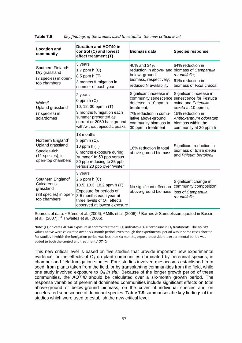
57

Page III - 57

Table 7.9 Key findings of the studies used to establish the new critical level.

Location and community

Duration and AOT40 in control (C) and lowest effect treatment (T)

Biomass data Species response

Southern Finland1 Dry grassland

(7 species) in open-top chambers

3 years

1.7 ppm h (C)

8.5 ppm h (T)

3 months fumigation in summer of each year

40% and 34% reduction in above- and below- ground biomass, respectively;

reduced N availability

64% reduction in biomass of Campanula rotundifolia;

61% reduction in biomass of Vicia cracca

Wales2 Upland grassland

(7 species) in solardomes

2 years

0 ppm h (C)

10, 12, 30 ppm h (T)

3 months fumigation each summer presented as current or 2050 background with/without episodic peaks

Significant increase in community senescence detected in 10 ppm h treatment;

7% reduction in cumu-lative above-ground community biomass in 30 ppm h treatment

Significant increase in senescence for Festuca ovina and Potentilla erecta at 10 ppm h;

15% reduction in Anthoxanthum odoratum biomass within the community at 30 ppm h

Northern England3 Upland grassland

Species-rich (11 species), in open-top chambers

18 months

3 ppm h (C).

10 ppm h (T)

6 months exposure during ‘summer’ to 50 ppb versus 30 ppb reducing to 35 ppb versus 20 ppb over ‘winter’

16% reduction in total above-ground biomass

Significant reduction in biomass of Briza media and Phleum bertolonii

Southern England4 Calcareous grassland

(38 species) in open-top chambers

3 years

2.6 ppm h (C)

10.5, 13.3, 18.2 ppm h (T)

Exposure for periods of 3-5 months each year at three levels of O3, effects observed at lowest exposure

No significant effect on above-ground biomass

Significant change in community composition;

loss of Campanula rotundifolia

Sources of data: 1 Rämö et al. (2006); 2 Mills et al. (2006); 3 Barnes & Samuelsson, quoted in Bassin et al. (2007); 4 Thwaites et al. (2006).

Note: (C) indicates AOT40 exposure in control treatment; (T) indicates AOT40 exposure in O3 treatments. The AOT40

values above were calculated over a six-month period, even though the experimental period was in some cases shorter.

For studies in which the fumigation period was less than six months, exposure outside the experimental period was

added to both the control and treatment AOT40.

This new critical level is based on five studies that provide important new experimental evidence for the effects of O3 on plant communities dominated by perennial species, in chamber and field fumigation studies. Four studies involved mesocosms established from seed, from plants taken from the field, or by transplanting communities from the field, while one study involved exposure to O3 in situ. Because of the longer growth period of these communities, the AOT40 should be calculated over a six-month growth period. The response variables of perennial dominated communities include significant effects on total above-ground or below-ground biomass, on the cover of individual species and on accelerated senescence of dominant species. Table 7.9 summarises the key findings of the studies which were used to establish the new critical level.

58

Page III - 58

Calculating exceedance of the AOT40-based critical level

Follow the procedure outlined in Section III.3.7.2 of the Modelling and Mapping Manual using the following recommendations specific to (semi-)natural vegetation:

Step 1: Determine the accumulation period

Ideally, a variable time-window should be used in the mapping procedure to account for different growth periods of annuals and perennials in different regions of Europe. The AOT40 is calculated over the first three or six months of the growing season. The start of the growing season can be identified using:

1. Appropriate phenological models;

2. Information from local or national experts;

3. The default table below (Table 7.10).

For some species, the most relevant period of the growing season for O3 effects may be less than three months in duration. In such cases, values of AOT40 should be calculated over the growing season, identified using appropriate local information.

Table 7.10 Default timing for the start and end of O3 exposure windows for (semi-)natural vegetation. (Note: regional classifications of countries are suggested in Table 7.2.

Region Start date End date (annual-dominated

communities)

End date (perennial-dominated

communities)

Eastern Mediterranean* 1 March 31 May 31 Aug

Western Mediterranean* 1 March 31 May 31 Aug

Continental Central Europe 1 April 30 June 30 Sept

Atlantic Central Europe 1 April 30 June 30 Sept

Northern Europe mid-April mid-July mid-October

* For mountain areas where the altitude is above 1500 m, use a start date of 1 April, with end dates of 30 June for

annual-dominated communities and 30 September for perennial-dominated communities.

Steps 2 and 3: Determine the O3 concentration at the top of the canopy

The AOT40 value should be calculated as the concentration at canopy height, using the information provided in Section III.3.4.2 of the Modelling and Mapping Manual and chapter 3 of this document. The transfer functions to make this calculation, based on deposition models, depend on a number of factors which may vary systematically between vegetation classes. These include canopy height and leaf area index (both natural variation and effects of management) and environmental variables such as vapour pressure deficit and soil moisture deficit. If such information is not available, it is recommended that the conversion factors for short grasslands are used as a default.

Steps 3 – 4: continue as indicated in III.3.7.2.

7.5 References

Ashmore, M.R. & Davison, A.W. (1996). Towards a critical level of ozone for natural vegetation. In: Kärenlampi, L. & Skärby, L., (Eds). (1996). Critical levels for ozone in Europe: testing and finalising the concepts. UNECE Workshop Report. University of Kuopio, Department of Ecology and Environmental Science, pp. 58-71.

59

Page III - 59

Bassin, S., Volk, M. & Fuhrer, J. (2007). Factors affecting the ozone sensitivity of temperate European grasslands: An overview. Environmental Pollution 146, 678-691.

Baumgarten, M., Werner, H., Häberle, K.H., Emberson, L., Fabian, P. & Matyssek, R. (2000). Seasonal ozone exposure of mature beech trees (Fagus sylvatica) at high altitude in the Bavarian forest (Germany) in comparison with young beech grown in the field and in phytotrons. Environmental Pollution 109, 431-442.

Bender, J., Bergmann, E., Dohrmann, A., Tebbe, C.C. & Weigel, H.J. (2002). Impact of ozone on plant competition and structural diversity of rhizosphere microbial communities in grassland mesocosms. Phyton 42, 7-12.

Franzaring, J., Tonneijck, A.E.G., Kooijman, A.W.N. & Dueck, T.A. (2000). Growth responses to ozone in plant species from wetlands. Environmental and Experimental Botany 44, 39-48.

Fuhrer, J. (1995). Integration of the ozone critical level approach in modelling activities. Background paper to the EMEP Workshop on the Control of Photochemical Oxidants over Europe, 24-27 October 1995 in St. Gallen, Switzerland. Federal Office of Environment, Forest and Landscape, Berne.

Fuhrer, J. & Achermann, B., (Eds). (1999). Critical Levels for Ozone – Level II. Swiss Agency for the Environment, Forests and Landscape, Berne. Environmental Documentation No. 115.

Fuhrer, J., Ashmore, M.R., Mills, G., Hayes, F. & Davison, A.W. (2003). Critical levels for semi-natural vegetation. In: Karlsson, P.E., Selldén, G. & Pleijel, H., (Eds). Establishing Ozone Critical Levels II. UNECE Workshop Report. IVL report B 1523. IVL Swedish Environmental Research Institute, Gothenburg, Sweden.

Fuhrer, J., Skärby, L. & Ashmore, M.R. (1997). Critical levels for ozone effects on vegetation in Europe. Environmental Pollution 97, 91-106.

Gelang, J., Pleijel, H., Sild, E., Danielsson, H., Younis, S. & Sellden, G. (2000). Rate and duration of grain filling in relation to flag leaf senescence and grain yield in spring wheat (Triticum aestivum) exposed to different concentrations of ozone. Physiologia Plantarum 110, 366-375.

Gimeno, B.S., Bermejo, V., Sanz, J., De La Torre, D. & Gil, J.M. (2003a). Ambient ozone levels induce adverse effects on the flower production of three clover species from Iberian Rangelands. In: Karlsson, P.E., Selldén, G. & Pleijel, H., (eds). Establishing Ozone Critical Levels II. UNECE Workshop Report. IVL report B 1523. IVL Swedish Environmental Research Institute, Gothenburg, Sweden.

Gimeno, B.S. Bermejo, V., Sanz, J., de la Torre, D. & Gil, J.M. (2004). Assessment of the effects of ozone exposure and plant competition on the reproductive ability of three therophytic clover species from Iberian pastures. Atmospheric Environment, 38, 2295 – 2303.

González-Fernández, I., Calvo, E., Gerosa, G., Bermejo, V., Marzuoli, R., Calatayud, V., Alonso, R. (2014). Setting ozone critical levels for protecting horticultural Mediterranean crops: Case study of tomato. Environmental Pollution 185, 178-187

Kärenlampi, L. & Skärby, L., (Eds). (1996). Critical levels for ozone in Europe: testing and finalising the concepts. UNECE Workshop Report. University of Kuopio, Department of Ecology and Environmental Science.

Karlsson, P.E., Uddling, J., Braun, S., Broadmeadow, M., Elvira, S., Gimeno, B.S., Le Thiec, D., Oksanen, E., Vandermeiren, K., Wilkinson, M. & Emberson, L. (2003). New critical levels for ozone impact on trees based on AOT40 and leaf cumulated uptake of ozone. In: Karlsson, P.E., Selldén, G. & Pleijel, H., (Eds). Establishing Ozone Critical Levels II. UNECE Workshop Report. IVL report B 1523. IVL Swedish Environmental Research Institute, Gothenburg, Sweden.

60

Page III - 60

Karlsson, P.E., Uddling, J., Braun, S., Broadmeadow, M., Elvira, S., Gimeno, B.S., Le Thiec, D., Oksanen, E., Vandermeiren, K., Wilkinson, M. & Emberson, L. (2004). New critical levels for ozone effects on young trees based on AOT40 and simulated cumulative leaf uptake of ozone. Atmospheric Environment 38, 2283 - 2294.

Manninen, S., Siivonen, N., Timonen, U. & Huttunen S. (2003). Differences in ozone response between two Finnish wild strawberry populations. Environmental and Experimental Botany 49, 29-39.

Mills, G., Buse, A., Gimeno, B., Bermejo, V., Holland, M., Emberson, L. & Pleijel, H. (2007). A synthesis of AOT40-based response functions and critical levels of ozone for agricultural and horticultural crops. Atmospheric Environment 41, 2630 – 2643.

Mills, G., Hayes, F., Simpson, D., Emberson, L., Norris, D., Harmens, H., Büker, P. (2011). Evidence of widespread effects of ozone on crops and (semi-)natural vegetation in Europe (1990–2006) in relation to AOT40- and flux-based risk maps. Global Change Biology 17, 592-613.

Mills, G., Hayes, F., Williams, P, Jones, M.L.M., Macmillan, R., Harmens, H., Lloyd, A. & Büker, P. (2006). Should the effects of increasing background ozone concentration on semi-natural vegetation communities be taken into account in revising the critical level? In: Wieser, G., and Tausz, M. (Eds). Proceedings of the workshop: Critical levels of ozone: further applying and developing the flux-based concept, Obergurgl, November, 2005.

Mills, G.E. & Ball, G.R. (1998). Annual Progress Report for the ICP-Crops (September 1997-August 1998). ICP-Crops Coordination Centre, CEH Bangor, UK.

Novak K., Skelly J.M., Schaub M., Kräuchi N., Hug C., Landolt W. & Bleuler, P. (2003). Ozone air pollution and foliar injury development on native plants of Switzerland. Environmental Pollution 125, 41 – 52.

Power, S.A. & Ashmore, M.R. (2002). Responses of fen and fen meadow communities to ozone. New Phytologist 156, 399-408.

Rämö, K., Kanerva, T., Nikula, S. Ojanperä, K. & Manninen, S. (2006). Influences of elevated ozone and carbon dioxide in growth responses of lowland hay meadow mesocosms. Environmental Pollution 144, 101-111.

Sanz, J., González-Fernández, I., Elvira, S., Muntifering, R., Alonso, R., Bermejo-Bermejo, V., 2016. Setting ozone critical levels for annual Mediterranean pasture species : Combined analysis of open-top chamber experiments. Science of the Total Environment 571, 670-679.

Simpson, D., Ashmore, M.R., Emberson, L., Tuovinen, J.P., 2007. A comparison of two different approaches for mapping potential ozone damage to vegetation. A model study. Environmental Pollution 146, 715-725.

Thwaites, R.H., Ashmore, M.R., Morton, A.J. & Pakeman, R.J. (2006). The effects of tropospheric ozone on the species dynamics of calcareous grasslands. Environmental Pollution 144, 500-509.

UNECE. (1996). Manual on methodologies and criteria for mapping critical levels/loads and geographical areas where they are exceeded. Texte 71/96, Umweltbundesamt, Berlin, Germany.

Van der Hayden D., Skelly J., Innes J., Hug, C., Zhang J., Landolt W. & Bleuler P. (2001). Ozone exposure thresholds and foliar injury on forest plants in Switzerland. Environmental Pollution 111, 321-331.

Wieser, G., & Tausz, M. (Eds), (2006). Proceedings of the workshop: Critical levels of ozone: further applying and developing the flux-based concept, Obergurgl, November, 2005.

Documents

SUPPLEMENT OF CHAPTER III (MAPPING CRITICAL LEVELS F ... · F. Hayes, CEH Bangor Shutterstock, UK Shutterstock, UK. 2 Chapter 3 was prepared under the leadership of the ICP Vegetation