Embed Size (px)
Citation preview
Supervised Hashing with Latent Factor Models
Peichao ZhangShanghai Key Laboratory of
Scalable Computing andSystems
Department of ComputerScience and Engineering
Shanghai Jiao Tong University,China
Wei ZhangShanghai Key Laboratory of
Scalable Computing andSystems
Department of ComputerScience and Engineering
Shanghai Jiao Tong University,China
Wu-Jun LiNational Key Laboratory forNovel Software TechnologyDepartment of ComputerScience and TechnologyNanjing University, [email protected]
Minyi GuoShanghai Key Laboratory of
Scalable Computing andSystems
Department of ComputerScience and Engineering
Shanghai Jiao Tong University,China
ABSTRACTDue to its low storage cost and fast query speed, hashinghas been widely adopted for approximate nearest neighborsearch in large-scale datasets. Traditional hashing methodstry to learn the hash codes in an unsupervised way wherethe metric (Euclidean) structure of the training data is pre-served. Very recently, supervised hashing methods, whichtry to preserve the semantic structure constructed from thesemantic labels of the training points, have exhibited higheraccuracy than unsupervised methods. In this paper, we pro-pose a novel supervised hashing method, called latent factorhashing (LFH), to learn similarity-preserving binary codesbased on latent factor models. An algorithm with conver-gence guarantee is proposed to learn the parameters of LFH.Furthermore, a linear-time variant with stochastic learningoptimization is proposed for training LFH on large-scaledatasets. Experimental results on two large datasets withsemantic labels show that LFH can achieve superior accu-racy than state-of-the-art methods with comparable trainingtime.
Categories and Subject DescriptorsH.3.3 [Information Storage And Retrieval]: Informa-tion Search and Retrieval—Retrieval models
Permission to make digital or hard copies of all or part of this work for personal orclassroom use is granted without fee provided that copies are not made or distributedfor profit or commercial advantage and that copies bear this notice and the full cita-tion on the first page. Copyrights for components of this work owned by others thanACM must be honored. Abstracting with credit is permitted. To copy otherwise, or re-publish, to post on servers or to redistribute to lists, requires prior specific permissionand/or a fee. Request permissions from [email protected]’14, July 6–11, 2014, Gold Coast, Queensland, Australia.Copyright 2014 ACM 978-1-4503-2257-7/14/07 ...$15.00.http://dx.doi.org/10.1145/2600428.2609600 .
KeywordsHashing; Latent Factor Model; Image Retrieval; Big Data
1. INTRODUCTIONNearest neighbor (NN) search plays a fundamental role in
machine learning and related areas, such as pattern recog-nition, information retrieval, data mining and computer vi-sion. In many real applications, it’s not necessary for analgorithm to return the exact nearest neighbors for everypossible query. Hence, in recent years approximate nearestneighbor (ANN) search algorithms with improved speed andmemory saving have been received more and more attentionby researchers [1, 2, 7].
Over the last decades, there has been an explosive growthof data from many areas. To meet the demand of perform-ing ANN search on these massive datasets, various hashingtechniques have been proposed due to their fast query speedand low storage cost [1, 4, 5, 8, 10, 16, 20, 21, 26, 27, 31,35, 36, 37, 38, 39, 40, 41]. The essential idea of hashing isto map the data points from the original feature space intobinary codes in the hashcode space with similarities betweenpairs of data points preserved. Hamming distance is usedto measure the closeness between binary codes, which is de-fined as the number of positions at which two binary codesdiffer. More specifically, when two data points are deemedas similar, their binary codes should have a low Hammingdistance. On the contrary, when two data points are dis-similar, a high Hamming distance is expected between theirbinary codes. The advantage of binary codes representationover the original feature vector representation is twofold.Firstly, each dimension of a binary code can be stored us-ing only 1 bit while several bytes are typically required forone dimension of the original feature vector, leading to adramatic reduction in storage cost. Secondly, by using bi-nary codes representation, all the data points within a spe-cific Hamming distance to a given query can be retrieved
173
in constant or sub-linear time regardless of the total size ofthe dataset [30]. Because of these two advantages, hashingtechniques have become a promising choice for efficient ANNsearch on massive datasets.Existing hashing methods can be divided into two cate-
gories: data-independent methods and data-dependent meth-ods [6, 17, 18]. For data-independent methods, the hash-ing functions are learned without using any training data.Representative data-independent methods include locality-sensitive hashing (LSH) [1, 5, 7], shift-invariant kernels hash-ing (SIKH) [22], and many other extensions [4, 13, 14]. Onthe other hand, for data-dependent methods, their hashingfunctions are learned from some training data. Generallyspeaking, data-dependent methods often require less num-ber of bits than data-independent methods to achieve satis-factory performance.The data-dependent methods can be further divided into
two categories: unsupervised and supervised methods [17,20, 32]. Unsupervised methods try to preserve the metric(Euclidean) structure between data points using only theirfeature information. Representative unsupervised methodsinclude spectral hashing (SH) [34], principal component anal-ysis based hashing (PCAH) [33], iterative quantization (ITQ)[6], anchor graph hashing (AGH) [18], isotropic hashing (Iso-Hash) [9], multimodel latent binary embedding (MLBE) [42]and predictable dual-view hashing (PDH) [23]. Due to thefact that high level semantic description of an object of-ten differs from the extracted low level feature descriptors,known as semantic gap [25], returning nearest neighborsaccording to metric distances between the feature vectorsdoesn’t always guarantee a good search quality. Hence,many recent works focus on supervised methods which tryto preserve the semantic structure among the data pointsby utilizing their associated semantic information [17, 19].Although there are also some works to exploit other typesof supervised information like the ranking information forhashing [16, 20], the semantic information is usually givenin the form of pairwise labels indicating whether two datapoints are known to be similar or dissimilar. Representa-tive supervised methods include restricted Boltzmann ma-chine based hashing (RBM) [24], binary reconstructive em-bedding (BRE) [12], sequential projection learning for hash-ing (SPLH) [33], minimal loss hashing (MLH) [19], kernel-based supervised hashing (KSH) [17], and linear discrimi-nant analysis based hashing (LDAHash) [28]. Additionally,there are also some semi-supervised hashing methods [32]which use both labeled data and unlabeled data to traintheir model. As stated in recent works [17, 19, 20], so-phisticated supervised methods, such as SPLH, MLH, andKSH, can achieve higher accuracy than unsupervised meth-ods. However, some existing supervised methods, like MLH,suffer from a very large amount of training time, making itdifficult to apply to large-scale datasets.In this paper, we propose a novel method, called latent
factor hashing (LFH), for supervised hashing. The maincontributions of this paper are outlined as follows:
• Base on latent factor models, the likelihood of the pair-wise similarities are elegantly modeled as a function ofthe Hamming distance between the corresponding datapoints.
• An algorithm with convergence guarantee is proposedto learn the parameters of LFH.
• To model the large-scale problems, a linear-time vari-ant with stochastic learning optimization is proposedfor fast parameter learning.
• Experimental results on two real datasets with seman-tic labels show that LFH can achieve much higher ac-curacy than other state-of-the-art methods with effi-ciency in training time.
The rest of the this paper is organized as follows: In Sec-tion 2, we will introduce the details of our LFH model. Ex-perimental results are presented in Section 3. Finally, weconclude the paper in Section 4.
2. LATENT FACTOR HASHINGIn this section, we present the details of our latent factor
hashing (LFH) model, including the model formulation andlearning algorithms.
2.1 Problem DefinitionSuppose we have N points as the training data, each rep-
resented as a feature vector xi ∈ RD. Some pairs of pointshave similarity labels sij associated, where sij = 1 meansxi and xj are similar and sij = 0 means xi and xj are dis-similar. Our goal is to learn a binary code bi ∈ {−1, 1}Qfor each xi with similarity between pairs preserved. In par-ticular, when sij = 1, the binary codes bi and bj shouldhave a low Hamming distance. On the other hand, whensij = 0, the Hamming distance between bi and bj shouldbe high. In compact form, we use a matrix X ∈ RN×D todenote all the feature vectors, a matrix B ∈ {−1, 1}N×Q todenote all the binary codes, and a set S = {sij} to denoteall the observed similarity labels. Additionally, we use thenotation Ai∗ and A∗j to denote the ith row and the jthcolumn of a matrix A, respectively. AT is the transposeof A. The similarity labels S can be constructed from theneighborhood structure by thresholding on the metric dis-tances between the feature vectors [17]. However, such S isof low quality since no semantic information is utilized. Insupervised hashing setting, S is often constructed from thesemantic labels within the data points. Such labels are oftenbuilt with manual effort to ensure its quality.
2.2 Model FormulationLet Θij denote half of the inner product between two bi-
nary codes bi,bj ∈ {−1, 1}Q:
Θij =1
2bTi bj .
The likelihood of the observed similarity labels S can bedefined as follows:
p(S | B) =∏
sij∈S
p(sij | B), (1)
with
p(sij | B) =
{aij , sij = 1
1− aij , sij = 0,
where aij = σ(Θij) with σ being the logistic function:
σ(x) =1
1 + e−x.
174
It is easy to prove the following relationship between theHamming distance distH(·, ·) and inner product of two bi-nary codes:
distH(bi,bj) =1
2(Q− bT
i bj) =1
2(Q− 2Θij).
We can find that the smaller the distH(bi,bj) is, the largerp(sij = 1 | B) will be. Maximizing the likelihood of S in(1) will make the Hamming distance between two similarpoints as small as possible, and that between two dissimilarpoints as high as possible. Hence this model is reasonableand matches the goal to preserve similarity.With some prior p(B), the posteriori of B can be com-
puted as follows:
p(B | S) ∼ p(S | B)p(B).
We can use maximum a posteriori estimation to learn theoptimalB. However, directly optimizing onB is an NP-hardproblem [34]. Following most existing hashing methods, wecompute the optimal B through two stages. In the firststage, we relax B to be a real valued matrix U ∈ RN×Q.The ith row of U is called the latent factor for the ith datapoint. We learn an optimal U under the same probabilisticframework as for B. Then in the second stage, we performsome rounding technique on the real valued U to get thebinary codes B.More specifically, we replace all the occurrences of B in
previous equations with U. Θij is then re-defined as:
Θij =1
2Ui∗U
Tj∗.
Similarly, p(S | B), p(B), p(B | S) are replaced with p(S | U),p(U), p(U | S), respectively. We put a normal distributionon p(U):
p(U) =
Q∏d=1
N (U∗d | 0, βI),
where N (·) denotes the normal distribution, I is an identitymatrix, and β is a hyper-parameter. The log posteriori ofU can then be derived as:
L = log p(U | S)
=∑
sij∈S
(sijΘij − log(1 + eΘij ))− 1
2β∥U∥2F + c, (2)
where ∥ · ∥F denotes the Frobenius norm of a matrix, andc is a constant term independent of U. The next step is tolearn the optimal U that maximizes L in (2).
2.3 LearningSince directly optimizing the whole U can be very time-
consuming, we optimize each row of U at a time with itsother rows fixed. We adopt the surrogate algorithm [15]to optimize each row Ui∗. The surrogate learning algo-rithm can be viewed as a generalization of the expectation-maximization (EM) algorithm. It constructs a lower boundof the objective function, and then updates the parametersto maximize that lower bound. Just like EM algorithm, weneed to derive different lower bounds and optimization pro-cedures for different models [15]. In the following content,we will derive the details of the surrogate learning algorithmfor our model.
The gradient vector and the Hessian matrix of the objec-tive function L defined in (2) with respect to Ui∗ can bederived as:
∂L
∂UTi∗
=1
2
∑j:sij∈S
(sij − aij)UTj∗
+1
2
∑j:sji∈S
(sji − aji)UTj∗ − 1
βUT
i∗,
∂2L
∂UTi∗∂Ui∗
=− 1
4
∑j:sij∈S
aij(1− aij)UTj∗Uj∗
− 1
4
∑j:sji∈S
aji(1− aji)UTj∗Uj∗ − 1
βI.
If we define Hi as:
Hi = − 1
16
∑j:sij∈S
UTj∗Uj∗ − 1
16
∑j:sji∈S
UTj∗Uj∗ − 1
βI, (3)
we can prove that
∂2L
∂UTi∗∂Ui∗
⪰ Hi,
whereA ⪰ BmeansA−B is a positive semi-definite matrix.Then we can construct the lower bound of L(Ui∗), de-
noted by L̃(Ui∗), as:
L̃(Ui∗) = L(Ui∗(t)) + (Ui∗ −Ui∗(t))∂L
∂UTi∗(t)
+1
2(Ui∗ −Ui∗(t))Hi(t)(Ui∗ −Ui∗(t))
T .
The values of U and other parameters that depend on Uchange through the updating process. Here we use the no-tation x(t) to denote the value of a parameter x at someiteration t. We update Ui∗ to be the one that gives the
maximum value of L̃(Ui∗). It is easy to see that L̃(Ui∗) is aquadratic form in the variable Ui∗, which can be proved tobe convex. Hence, we can find the optimum value of Ui∗ by
setting the gradient of L̃(Ui∗) with respect to Ui∗ to 0. Asa result, we end up with the following update rule for Ui∗:
Ui∗(t+ 1) = Ui∗(t)− [∂L
∂UTi∗(t)]THi(t)
−1. (4)
We can then update other rows of U iteratively using theabove rule.
The convergence of the iterative updating process is con-trolled by some threshold value ε and the maximum allowednumber of iterations T . Here ε and T are both hyper-parameters. During each iteration, we update U by up-dating each of its rows sequentially. The initial value of Ucan be obtained through PCA on the feature space X. Thepseudocode of the updating process is shown in Algorithm 1.
2.3.1 RoundingAfter the optimal U is learned, we can obtain the final
binary codes B using some rounding techniques. In thispaper, to keep our method simple, the real values of U arequantized into the binary codes of B by taking their signs,that is:
Bij =
{1, Uij > 0
−1, otherwise.
175
Algorithm 1 Optimizing U using surrogate algorithm
Input: X ∈ RN×D,S = {sij}, Q, T ∈ N+, β, ε ∈ R+.Initializing U by performing PCA on X.for t = 1 → T do
for i = 1 → N doUpdate Ui∗ by following the rule given in (4).
end forCompute L in (2) using the updated U.Terminate the iterative process when the change of Lis smaller than ε.
end forOutput: U ∈ RN×Q.
2.3.2 Out-of-Sample ExtensionIn order to perform ANN search, we need to compute the
binary code b for a query x which is not in the training set.We achieve this by finding a matrix W ∈ RD×Q that mapsx to u in the following way:
u = WTx.
We then perform the same rounding technique discussed inSection 2.3.1 on u to obtain b.We use linear regression to train W over the training set.
The squared loss with regularization term is shown below:
Le = ∥U−XW∥2F + λe∥W∥2F .
And the optimal W can be computed as:
W = (XTX+ λeI)−1XTU. (5)
2.4 Convergence and Complexity AnalysisAt each iteration, we first construct a lower bound at the
current point Ui∗(t), and then optimize it to get a newpoint Ui∗(t+1) with a higher function value L(Ui∗(t+1)).Hence, the objective function value always increases in thenew iteration. Furthermore, the objective function valueL = log p(U | S) is upper bounded by zero. Hence, our Al-gorithm 1 can always guarantee convergence to local maxi-mum, the principle of which is similar to that of EM algo-rithm. This convergence property will also be illustrated inFigure 2. The convergence property of our surrogate algo-rithm is one of the key advantages compared with standardNewton method and first-order gradient method. In bothNewton method and first-order gradient method, a step size,also called learning rate in some literatures, should be man-ually specified, which cannot necessarily guarantee conver-gence.We can prove that, when updating Ui∗, the total time to
compute ∂L/∂UTi∗ and Hi for all i = 1, . . . , N is O(|S|Q)
and O(|S|Q2), respectively. Since the inversion of Hi can becomputed in O(Q3), the time to update Ui∗ following therule given in (4) is O(Q3). Then the time to update U byone iteration is O(NQ3 + |S|Q2). Therefore, the total timeof the updating process is O(T (NQ3 + |S|Q2)), where T isthe number of iterations.Besides that, the time for rounding is O(NQ). And the
time to compute W for out-of-sample extension is O(ND2+D3+NDQ), which can be further reduced to O(ND2) withthe typical assumption that Q < D ≪ N . With the pre-computed W, the out-of-sample extension for a query x canbe achieved in O(DQ).
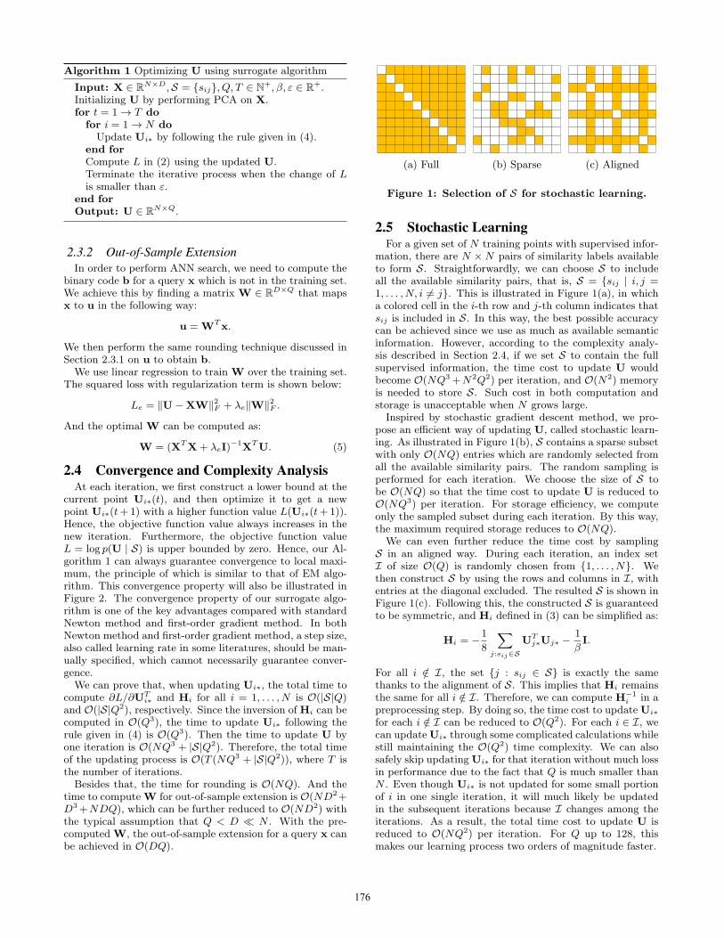
(a) Full (b) Sparse (c) Aligned
Figure 1: Selection of S for stochastic learning.
2.5 Stochastic LearningFor a given set of N training points with supervised infor-
mation, there are N ×N pairs of similarity labels availableto form S. Straightforwardly, we can choose S to includeall the available similarity pairs, that is, S = {sij | i, j =1, . . . , N, i ̸= j}. This is illustrated in Figure 1(a), in whicha colored cell in the i-th row and j-th column indicates thatsij is included in S. In this way, the best possible accuracycan be achieved since we use as much as available semanticinformation. However, according to the complexity analy-sis described in Section 2.4, if we set S to contain the fullsupervised information, the time cost to update U wouldbecome O(NQ3+N2Q2) per iteration, and O(N2) memoryis needed to store S. Such cost in both computation andstorage is unacceptable when N grows large.
Inspired by stochastic gradient descent method, we pro-pose an efficient way of updating U, called stochastic learn-ing. As illustrated in Figure 1(b), S contains a sparse subsetwith only O(NQ) entries which are randomly selected fromall the available similarity pairs. The random sampling isperformed for each iteration. We choose the size of S tobe O(NQ) so that the time cost to update U is reduced toO(NQ3) per iteration. For storage efficiency, we computeonly the sampled subset during each iteration. By this way,the maximum required storage reduces to O(NQ).
We can even further reduce the time cost by samplingS in an aligned way. During each iteration, an index setI of size O(Q) is randomly chosen from {1, . . . , N}. Wethen construct S by using the rows and columns in I, withentries at the diagonal excluded. The resulted S is shown inFigure 1(c). Following this, the constructed S is guaranteedto be symmetric, and Hi defined in (3) can be simplified as:
Hi = −1
8
∑j:sij∈S
UTj∗Uj∗ − 1
βI.
For all i /∈ I, the set {j : sij ∈ S} is exactly the samethanks to the alignment of S. This implies that Hi remainsthe same for all i /∈ I. Therefore, we can compute H−1
i in apreprocessing step. By doing so, the time cost to updateUi∗for each i /∈ I can be reduced to O(Q2). For each i ∈ I, wecan updateUi∗ through some complicated calculations whilestill maintaining the O(Q2) time complexity. We can alsosafely skip updatingUi∗ for that iteration without much lossin performance due to the fact that Q is much smaller thanN . Even though Ui∗ is not updated for some small portionof i in one single iteration, it will much likely be updatedin the subsequent iterations because I changes among theiterations. As a result, the total time cost to update U isreduced to O(NQ2) per iteration. For Q up to 128, thismakes our learning process two orders of magnitude faster.
176
Consequently, since Q is bounded by a small constant,we can say that the cost in computation and storage ofour learning algorithm are linear to the number of train-ing points N . This makes our LFH easily scalable to verylarge datasets.
2.6 Normalized Hyper-parametersThe hyper-parameter β in the objective function defined
in (2) acts as a factor weighing the relative importance be-tween the first and the second term. However, the numberof sum items in each term is different: in the first term thereare |S| sum items, while in the second term there are N sumitems. Since different datasets may have different values ofN and |S|, the optimal value of β may vary between thedatasets. To address this issue and make our method lessdependent on a specific dataset, we introduce a new hyper-parameter β′ satisfying that:
β′ =N
|S|β.
By replacing β with β′ in (2), we have a specialized param-eter β′ for each dataset. The optimal value for β is thennormalized to roughly the same range on different datasets.We can normalize λe in (5) by following the same idea.We find that the MLH method spends most of the time
on selecting the best hyper-parameters for each dataset.With the normalized hyper-parameters introduced, we canpre-compute the optimal values for the hyper-parameterson some smaller dataset, and then apply the same valuesto all other datasets. This saves us the time of hyper-parameter selection and makes our method more efficienton large datasets.
3. EXPERIMENT
3.1 DatasetsWe evaluate our method on two standard large image
datasets with semantic labels: CIFAR-10 [11] and NUS-WIDE [3].The CIFAR-10 dataset [11] consists of 60,000 color images
drawn from the 80M tiny image collection [29]. Each imageof size 32 × 32 is represented by a 512-dimensional GISTfeature vector. Each image is manually classified into oneof the 10 classes, with an exclusive label indicating its be-longing class. Two images are considered as a ground truthneighbor if they have the same class label.The NUS-WIDE dataset [3] contains 269,648 images col-
lected from Flickr. Each image is represented by a 1134-dimensional low level feature vector, including color his-togram, color auto-correlogram, edge direction histogram,wavelet texture, block-wise color moments, and bag of vi-sual words. The images are manually assigned with some ofthe 81 concept tags. The ground truth neighbor is definedon two images if they share at least one common tag.For data pre-processing, we follow the standard way of
feature normalization by making each dimension of the fea-ture vectors to have zero mean and equal variance.
3.2 Experimental Settings and BaselinesFor both CIFAR-10 and NUS-WIDE datasets, we ran-
domly sample 1,000 points as query set, 1,000 points as val-idation set, and all the remaining points as training set. Us-ing normalized hyper-parameters described in Section 2.6,
the best hyper-parameters are selected by using the valida-tion set of CIFAR-10. All experimental results are averagedover 10 independent rounds of random training / validation/ query partitions.
Unless otherwise stated, we refer LFH in the experimentsection to the LFH with stochastic learning. We compareour LFH method with some state-of-the-art hashing meth-ods, which include:
• Data-independent methods: locality-sensitive hashing(LSH), and shift-invariant kernels hashing (SIKH);
• Unsupervised data-dependent methods: spectral hash-ing (SH), principal component analysis based hash-ing (PCAH), iterative quantization (ITQ), anchor graphhashing (AGH);
• Supervised data-dependent methods: sequential pro-jection learning for hashing (SPLH), minimal loss hash-ing (MLH), and kernel-based supervised hashing (KSH).
All the baseline methods are implemented using the sourcecodes provided by the corresponding authors. For KSH andAGH, the number of support points for kernel constructionis set to 300 by following the same settings in [17, 18]. ForKSH, SPLH, and MLH, it’s impossible to use all the super-vised information for training since it would be very time-consuming. Following the same strategy used in [17], wesample 2,000 labeled points for these methods.
All our experiments are conducted on a workstation with24 Intel Xeon CPU cores and 64 GB RAM.
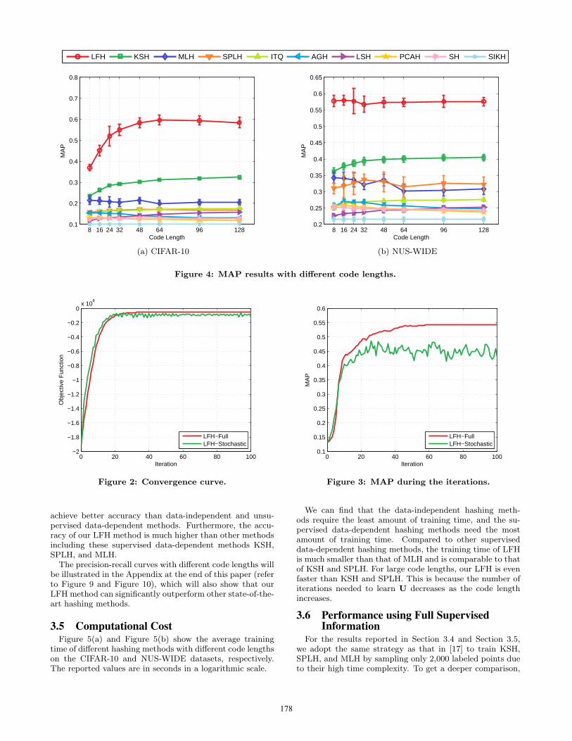
3.3 Effect of Stochastic LearningThe convergence curve of the objective function on a sam-
pled CIFAR-10 subset of 5000 points with code length 32 isshown in Figure 2. The LFH-Full method refers to the LFHthat uses the full supervised information for updating, andLFH-Stochastic refers to the LFH with stochastic learning.The objective function value is computed based on the fullsupervised information for both methods. We can see thatthe objective function of LFH-Full converges to a station-ary point after a few iterations. The objective function ofLFH-Stochastic has a major trend of convergence to somestationary point with slight vibration. This behavior is quitesimilar to stochastic gradient descent method and is empir-ically acceptable.
Figure 3 shows the mean average precision (MAP) [10, 17,19] values computed on a validation set during the updatingprocess. The final MAP evaluated on a query set is 0.5237for LFH-Full and 0.4694 for LFH-Stochastic. The reductionin MAP of LFH-Stochastic is affordable given the dramaticdecrease in time complexity by using stochastic learning.
3.4 Hamming Ranking PerformanceWe perform Hamming ranking using the generated binary
codes on the CIFAR-10 and NUS-WIDE datasets. For eachquery in the query set, all the points in the training set areranked according to the Hamming distance between theirbinary codes and the query’s. The MAP is reported to eval-uate the accuracy of different hashing methods.
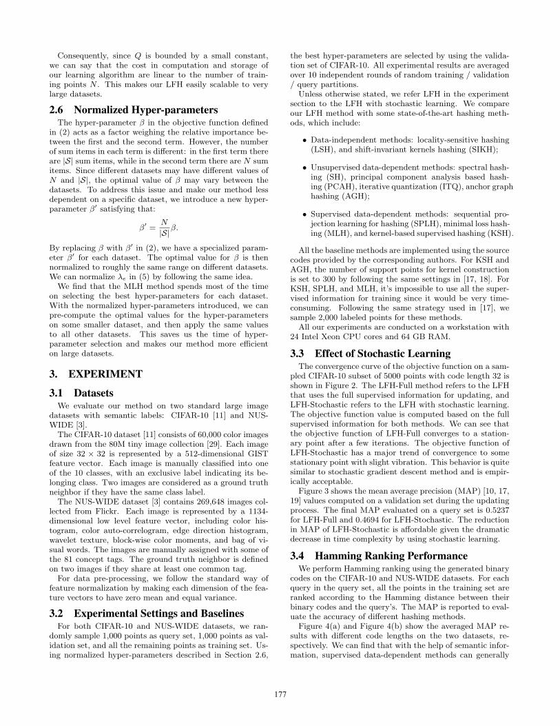
Figure 4(a) and Figure 4(b) show the averaged MAP re-sults with different code lengths on the two datasets, re-spectively. We can find that with the help of semantic infor-mation, supervised data-dependent methods can generally
177
LFH KSH MLH SPLH ITQ AGH LSH PCAH SH SIKH
8 16 24 32 48 64 96 1280.1
0.2
0.3
0.4
0.5
0.6
0.7
0.8
Code Length
MA
P
(a) CIFAR-10
8 16 24 32 48 64 96 1280.2
0.25
0.3
0.35
0.4
0.45
0.5
0.55
0.6
0.65
Code Length
MA
P
(b) NUS-WIDE
Figure 4: MAP results with different code lengths.
0 20 40 60 80 100−2
−1.8
−1.6
−1.4
−1.2
−1
−0.8
−0.6
−0.4
−0.2
0x 10
8
Iteration
Obj
ectiv
e F
unct
ion
LFH−FullLFH−Stochastic
Figure 2: Convergence curve.
achieve better accuracy than data-independent and unsu-pervised data-dependent methods. Furthermore, the accu-racy of our LFH method is much higher than other methodsincluding these supervised data-dependent methods KSH,SPLH, and MLH.The precision-recall curves with different code lengths will
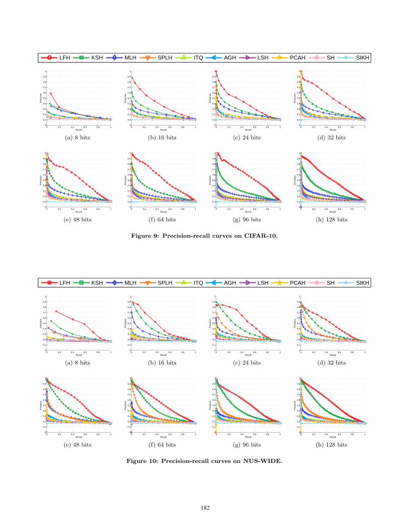
be illustrated in the Appendix at the end of this paper (referto Figure 9 and Figure 10), which will also show that ourLFH method can significantly outperform other state-of-the-art hashing methods.
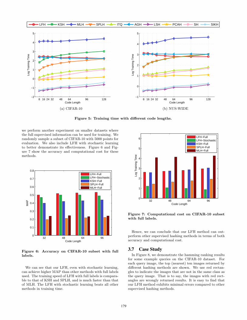
3.5 Computational CostFigure 5(a) and Figure 5(b) show the average training
time of different hashing methods with different code lengthson the CIFAR-10 and NUS-WIDE datasets, respectively.The reported values are in seconds in a logarithmic scale.
0 20 40 60 80 1000.1
0.15
0.2
0.25
0.3
0.35
0.4
0.45
0.5
0.55
0.6
Iteration
MA
P
LFH−FullLFH−Stochastic
Figure 3: MAP during the iterations.
We can find that the data-independent hashing meth-ods require the least amount of training time, and the su-pervised data-dependent hashing methods need the mostamount of training time. Compared to other superviseddata-dependent hashing methods, the training time of LFHis much smaller than that of MLH and is comparable to thatof KSH and SPLH. For large code lengths, our LFH is evenfaster than KSH and SPLH. This is because the number ofiterations needed to learn U decreases as the code lengthincreases.
3.6 Performance using Full SupervisedInformation
For the results reported in Section 3.4 and Section 3.5,we adopt the same strategy as that in [17] to train KSH,SPLH, and MLH by sampling only 2,000 labeled points dueto their high time complexity. To get a deeper comparison,
178
LFH KSH MLH SPLH ITQ AGH LSH PCAH SH SIKH
8 16 24 32 48 64 96 128−2
−1
0
1
2
3
4
5
Code Length
Log
Tra
inin
g T
ime
(a) CIFAR-10
8 16 24 32 48 64 96 128−1
0
1
2
3
4
5
Code Length
Log
Tra
inin
g T
ime
(b) NUS-WIDE
Figure 5: Training time with different code lengths.
we perform another experiment on smaller datasets wherethe full supervised information can be used for training. Werandomly sample a subset of CIFAR-10 with 5000 points forevaluation. We also include LFH with stochastic learningto better demonstrate its effectiveness. Figure 6 and Fig-ure 7 show the accuracy and computational cost for thesemethods.
32 48 64 960
0.1
0.2
0.3
0.4
0.5
0.6
0.7
0.8
Code Length
MA
P
LFH−FullLFH−StochasticKSH−FullSPLH−FullMLH−Full
Figure 6: Accuracy on CIFAR-10 subset with fulllabels.
We can see that our LFH, even with stochastic learning,can achieve higher MAP than other methods with full labelsused. The training speed of LFH with full labels is compara-ble to that of KSH and SPLH, and is much faster than thatof MLH. The LFH with stochastic learning beats all othermethods in training time.
32 48 64 960
1
2
3
4
5
6
Code Length
Log
Tra
inin
g T
ime
LFH−FullLFH−StochasticKSH−FullSPLH−FullMLH−Full
Figure 7: Computational cost on CIFAR-10 subsetwith full labels.
Hence, we can conclude that our LFH method can out-perform other supervised hashing methods in terms of bothaccuracy and computational cost.
3.7 Case StudyIn Figure 8, we demonstrate the hamming ranking results
for some example queries on the CIFAR-10 dataset. Foreach query image, the top (nearest) ten images returned bydifferent hashing methods are shown. We use red rectan-gles to indicate the images that are not in the same class asthe query image. That is to say, the images with red rect-angles are wrongly returned results. It is easy to find thatour LFH method exhibits minimal errors compared to othersupervised hashing methods.
179

(a)
(b)
(c) (d)
(e) (f)
Figure 8: Example search (Hamming ranking) results on CIFAR-10, where red rectangles are used to indicatethe images that are not in the same class as the query image, i.e., the wrongly returned results. (a) and(b) contain the same query images, which are duplicated for better demonstration. Other images are thereturned results of (c) LFH; (d) KSH; (e) MLH; (f) SPLH.
4. CONCLUSIONHashing has become a very effective technique for ANN
search in massive datasets which are common in this bigdata era. In many datasets, it is not hard to collect somesupervised information, such as the tag information in manysocial web sites, for part of the whole dataset. Hence, su-pervised hashing methods, which can outperform traditionalunsupervised hashing methods, have become more and moreimportant. In this paper, we propose a novel method, calledLFH, for supervised hashing. A learning algorithm with con-vergence guarantee is proposed to learn the parameters ofLFH. Moreover, to model large-scale problems, we propose astochastic learning method which has linear time complexity.Experimental results on two large datasets with semanticlabels show that our LFH method can achieve higher accu-racy than other state-of-the-art methods with comparableor lower training cost.
5. ACKNOWLEDGMENTSThis work is supported by the NSFC (No. 61100125,
61272099, 61261160502), the 863 Program of China (No.2012AA011003), Shanghai Excellent Academic Leaders Plan(No. 11XD1402900), Scientific Innovation Act of STCSM(No. 13511504200), and the Program for Changjiang Schol-ars and Innovative Research Team in University of China(IRT1158, PCSIRT).
6. REFERENCES[1] A. Andoni and P. Indyk. Near-optimal hashing algorithms
for approximate nearest neighbor in high dimensions. In
Proceedings of the Annual Symposium on Foundations ofComputer Science, pages 459–468, 2006.
[2] S. Arya, D. M. Mount, N. S. Netanyahu, R. Silverman, andA. Y. Wu. An optimal algorithm for approximate nearestneighbor searching fixed dimensions. Journal of the ACM,45(6):891–923, 1998.
[3] T.-S. Chua, J. Tang, R. Hong, H. Li, Z. Luo, and Y. Zheng.Nus-wide: A real-world web image database from nationaluniversity of singapore. In Proceedings of the ACMInternational Conference on Image and Video Retrieval,2009.
[4] M. Datar, N. Immorlica, P. Indyk, and V. S. Mirrokni.Locality-sensitive hashing scheme based on p-stabledistributions. In Proceedings of the Annual Symposium onComputational Geometry, pages 253–262, 2004.
[5] A. Gionis, P. Indyk, and R. Motwani. Similarity search inhigh dimensions via hashing. In Proceedings of theInternational Conference on Very Large Data Bases, pages518–529, 1999.
[6] Y. Gong and S. Lazebnik. Iterative quantization: Aprocrustean approach to learning binary codes. InProceedings of the IEEE Computer Society Conference onComputer Vision and Pattern Recognition, pages 817–824,2011.
[7] P. Indyk and R. Motwani. Approximate nearest neighbors:Towards removing the curse of dimensionality. InProceedings of the Annual ACM Symposium on Theory ofComputing, pages 604–613, 1998.
[8] W. Kong and W.-J. Li. Double-bit quantization forhashing. In Proceedings of the AAAI Conference onArtificial Intelligence, 2012.
[9] W. Kong and W.-J. Li. Isotropic hashing. In Proceedings ofthe Annual Conference on Neural Information ProcessingSystems, pages 1655–1663, 2012.
180
[10] W. Kong, W.-J. Li, and M. Guo. Manhattan hashing forlarge-scale image retrieval. In Proceedings of theInternational ACM SIGIR Conference on Research andDevelopment in Information Retrieval, pages 45–54, 2012.
[11] A. Krizhevsky. Learning multiple layers of features fromtiny images. Master’s thesis, University of Toronto, 2009.
[12] B. Kulis and T. Darrell. Learning to hash with binaryreconstructive embeddings. In Proceedings of the AnnualConference on Neural Information Processing Systems,pages 1042–1050, 2009.
[13] B. Kulis and K. Grauman. Kernelized locality-sensitivehashing for scalable image search. In Proceedings of theIEEE International Conference on Computer Vision, pages2130–2137, 2009.
[14] B. Kulis, P. Jain, and K. Grauman. Fast similarity searchfor learned metrics. IEEE Transactions on PatternAnalysis and Machine Intelligence, 31(12):2143–2157, 2009.
[15] K. Lange, D. R. Hunter, and I. Yang. Optimization transferusing surrogate objective functions. Journal ofComputational and Graphical Statistics, 9(1):1–20, 2000.
[16] X. Li, G. Lin, C. Shen, A. van den Hengel, and A. R. Dick.Learning hash functions using column generation. InProceedings of the International Conference on MachineLearning, pages 142–150, 2013.
[17] W. Liu, J. Wang, R. Ji, Y.-G. Jiang, and S.-F. Chang.Supervised hashing with kernels. In Proceedings of theIEEE Computer Society Conference on Computer Visionand Pattern Recognition, pages 2074–2081, 2012.
[18] W. Liu, J. Wang, S. Kumar, and S.-F. Chang. Hashingwith graphs. In Proceedings of the International Conferenceon Machine Learning, 2011.
[19] M. Norouzi and D. J. Fleet. Minimal loss hashing forcompact binary codes. In Proceedings of the InternationalConference on Machine Learning, pages 353–360, 2011.
[20] M. Norouzi, D. J. Fleet, and R. Salakhutdinov. Hammingdistance metric learning. In Proceedings of the AnnualConference on Neural Information Processing Systems,pages 1070–1078, 2012.
[21] M. Ou, P. Cui, F. Wang, J. Wang, W. Zhu, and S. Yang.Comparing apples to oranges: A scalable solution withheterogeneous hashing. In Proceedings of the ACMSIGKDD International Conference on KnowledgeDiscovery and Data Mining, pages 230–238, 2013.
[22] M. Raginsky and S. Lazebnik. Locality-sensitive binarycodes from shift-invariant kernels. In Proceedings of theAnnual Conference on Neural Information ProcessingSystems, pages 1509–1517, 2009.
[23] M. Rastegari, J. Choi, S. Fakhraei, D. Hal, and L. S. Davis.Predictable dual-view hashing. In Proceedings of theInternational Conference on Machine Learning, pages1328–1336, 2013.
[24] R. Salakhutdinov and G. E. Hinton. Semantic hashing.International Journal of Approximate Reasoning,50(7):969–978, 2009.
[25] A. W. M. Smeulders, M. Worring, S. Santini, A. Gupta,and R. Jain. Content-based image retrieval at the end ofthe early years. IEEE Transactions on Pattern Analysisand Machine Intelligence, 22(12):1349–1380, 2000.
[26] J. Song, Y. Yang, Y. Yang, Z. Huang, and H. T. Shen.Inter-media hashing for large-scale retrieval fromheterogeneous data sources. In Proceedings of the ACMSIGMOD International Conference on Management ofData, pages 785–796, 2013.
[27] B. Stein. Principles of hash-based text retrieval. InProceedings of the International ACM SIGIR Conferenceon Research and Development in Information Retrieval,pages 527–534, 2007.
[28] C. Strecha, A. A. Bronstein, M. M. Bronstein, and P. Fua.Ldahash: Improved matching with smaller descriptors.IEEE Transactions on Pattern Analysis and MachineIntelligence, 34(1):66–78, 2012.
[29] A. Torralba, R. Fergus, and W. T. Freeman. 80 million tinyimages: A large data set for nonparametric object andscene recognition. IEEE Transactions on Pattern Analysisand Machine Intelligence, 30(11):1958–1970, 2008.
[30] A. Torralba, R. Fergus, and Y. Weiss. Small codes andlarge image databases for recognition. In Proceedings of theIEEE Computer Society Conference on Computer Visionand Pattern Recognition, 2008.
[31] F. Ture, T. Elsayed, and J. J. Lin. No free lunch: Bruteforce vs. locality-sensitive hashing for cross-lingual pairwisesimilarity. In Proceedings of the International ACM SIGIRConference on Research and Development in InformationRetrieval, pages 943–952, 2011.
[32] J. Wang, O. Kumar, and S.-F. Chang. Semi-supervisedhashing for scalable image retrieval. In Proceedings of theIEEE Computer Society Conference on Computer Visionand Pattern Recognition, pages 3424–3431, 2010.
[33] J. Wang, S. Kumar, and S.-F. Chang. Sequential projectionlearning for hashing with compact codes. In Proceedings ofthe International Conference on Machine Learning, pages1127–1134, 2010.
[34] Y. Weiss, A. Torralba, and R. Fergus. Spectral hashing. InProceedings of the Annual Conference on NeuralInformation Processing Systems, pages 1753–1760, 2008.
[35] F. Wu, Z. Yu, Y. Yang, S. Tang, Y. Zhang, and Y. Zhuang.Sparse multi-modal hashing. IEEE Transactions onMultimedia, 16(2):427–439, 2014.
[36] B. Xu, J. Bu, Y. Lin, C. Chen, X. He, and D. Cai.Harmonious hashing. In Proceedings of the InternationalJoint Conference on Artificial Intelligence, 2013.
[37] D. Zhai, H. Chang, Y. Zhen, X. Liu, X. Chen, and W. Gao.Parametric local multimodal hashing for cross-viewsimilarity search. In Proceedings of the International JointConference on Artificial Intelligence, 2013.
[38] D. Zhang and W.-J. Li. Large-scale supervised multimodalhashing with semantic correlation maximization. InProceedings of the AAAI Conference on ArtificialIntelligence, 2014.
[39] D. Zhang, F. Wang, and L. Si. Composite hashing withmultiple information sources. In Proceedings of theInternational ACM SIGIR Conference on Research andDevelopment in Information Retrieval, pages 225–234,2011.
[40] D. Zhang, J. Wang, D. Cai, and J. Lu. Self-taught hashingfor fast similarity search. In Proceedings of theInternational ACM SIGIR Conference on Research andDevelopment in Information Retrieval, pages 18–25, 2010.
[41] Q. Zhang, Y. Wu, Z. Ding, and X. Huang. Learning hashcodes for efficient content reuse detection. In Proceedings ofthe International ACM SIGIR Conference on Research andDevelopment in Information Retrieval, pages 405–414,2012.
[42] Y. Zhen and D.-Y. Yeung. A probabilistic model formultimodal hash function learning. In Proceedings of theACM SIGKDD International Conference on KnowledgeDiscovery and Data Mining, pages 940–948, 2012.
APPENDIXFor a more extensive evaluation, in Figure 9 and Figure 10,we illustrate the precision-recall curves with different codelengths on the two datasets, CIFAR-10 and NUS-WIDE.Our LFH method shows clear superiority on almost all set-tings, followed by KSH, SPLH, and MLH, and then the othermethods without using semantic information. The resultsare consistent with the MAP results given above.
181
LFH KSH MLH SPLH ITQ AGH LSH PCAH SH SIKH
0 0.2 0.4 0.6 0.8 10
0.1
0.2
0.3
0.4
0.5
0.6
0.7
0.8
0.9
1
Recall
Pre
cisi
on
(a) 8 bits
0 0.2 0.4 0.6 0.8 10
0.1
0.2
0.3
0.4
0.5
0.6
0.7
0.8
0.9
1
Recall
Pre
cisi
on
(b) 16 bits
0 0.2 0.4 0.6 0.8 10
0.1
0.2
0.3
0.4
0.5
0.6
0.7
0.8
0.9
1
Recall
Pre
cisi
on
(c) 24 bits
0 0.2 0.4 0.6 0.8 10
0.1
0.2
0.3
0.4
0.5
0.6
0.7
0.8
0.9
1
Recall
Pre
cisi
on
(d) 32 bits
0 0.2 0.4 0.6 0.8 10
0.1
0.2
0.3
0.4
0.5
0.6
0.7
0.8
0.9
1
Recall
Pre
cisi
on
(e) 48 bits
0 0.2 0.4 0.6 0.8 10
0.1
0.2
0.3
0.4
0.5
0.6
0.7
0.8
0.9
1
Recall
Pre
cisi
on
(f) 64 bits
0 0.2 0.4 0.6 0.8 10
0.1
0.2
0.3
0.4
0.5
0.6
0.7
0.8
0.9
1
RecallP
reci
sion
(g) 96 bits
0 0.2 0.4 0.6 0.8 10
0.1
0.2
0.3
0.4
0.5
0.6
0.7
0.8
0.9
1
Recall
Pre
cisi
on
(h) 128 bits
Figure 9: Precision-recall curves on CIFAR-10.
LFH KSH MLH SPLH ITQ AGH LSH PCAH SH SIKH
0 0.2 0.4 0.6 0.8 10
0.1
0.2
0.3
0.4
0.5
0.6
0.7
0.8
0.9
1
Recall
Pre
cisi
on
(a) 8 bits
0 0.2 0.4 0.6 0.8 10
0.1
0.2
0.3
0.4
0.5
0.6
0.7
0.8
0.9
1
Recall
Pre
cisi
on
(b) 16 bits
0 0.2 0.4 0.6 0.8 10
0.1
0.2
0.3
0.4
0.5
0.6
0.7
0.8
0.9
1
Recall
Pre
cisi
on
(c) 24 bits
0 0.2 0.4 0.6 0.8 10
0.1
0.2
0.3
0.4
0.5
0.6
0.7
0.8
0.9
1
Recall
Pre
cisi
on
(d) 32 bits
0 0.2 0.4 0.6 0.8 10
0.1
0.2
0.3
0.4
0.5
0.6
0.7
0.8
0.9
1
Recall
Pre
cisi
on
(e) 48 bits
0 0.2 0.4 0.6 0.8 10
0.1
0.2
0.3
0.4
0.5
0.6
0.7
0.8
0.9
1
Recall
Pre
cisi
on
(f) 64 bits
0 0.2 0.4 0.6 0.8 10
0.1
0.2
0.3
0.4
0.5
0.6
0.7
0.8
0.9
1
Recall
Pre
cisi
on
(g) 96 bits
0 0.2 0.4 0.6 0.8 10
0.1
0.2
0.3
0.4
0.5
0.6
0.7
0.8
0.9
1
Recall
Pre
cisi
on
(h) 128 bits
Figure 10: Precision-recall curves on NUS-WIDE.
182