SUPERSYMMETRIC SU(5) U(1) MODEL AND QUARK …wtang/Main-Book.pdf · AND QUARK YUKAWA COUPLINGS Walter Orlando Tangarife Garc´ıa Advisor: Diego Alejandro Restrepo. Presented to obtain

SUPERSYMMETRIC SU(5)× U(1) MODELAND QUARK YUKAWA COUPLINGS

Walter Orlando Tangarife Garcıa

Advisor:Diego Alejandro Restrepo.

Presented to obtain the degree of

Physicist

Universidad de AntioquiaFacultad de Ciencias Exactas y Naturales

Instituto de FısicaGrupo de Fenomenologıa de Interacciones Fundamentales

Medellın2008

To Edilma Garcıa

Abstract

The Standard Model (SM) of elementary particles, in spite of its great success,does not address some fundamental questions, namely the different couplings forthe subatomic interactions, the amount of parameters in the model, the quanti-zation of the charge and the hierarchy problem. Glashow and Georgi proposeda model in which the strong, weak and electromagnetic interactions unify underonly one gauge group: SU(5). The minimal SU(5) model is not consistent withinthe gauge couplings evolution nor with experimental data about proton decay.The supersymmetric extension of SU(5) solves these problems and yields a moreconsistent model. In this work we study the general features of the supersym-metric SU(5) model and analise the fermion mass hierarchy problem. In oder totackle this problem, we implement a mechanism a la Froggatt-Nielsen assumingthat at the GUT scale a horizontal U(1)H global flavour symmetry is unbroken.As a result of breaking the horizontal symmetry through an SU(5) adjoint, weobtain the Yukawa couplings for the down-type quarks and some couplings forthe up-type quarks as well.

i

Contents

1 SU(5) Grand Unified Theory 3

1.1 Puzzles in the Standard Model . . . . . . . . . . . . . . . . . . . . 31.2 The SU(5) Model . . . . . . . . . . . . . . . . . . . . . . . . . . . 5

1.2.1 The group choice and representations . . . . . . . . . . . . 51.2.2 Spontaneous symmetry breaking . . . . . . . . . . . . . . . 101.2.3 SU(5) Lagrangian and gauge vertices . . . . . . . . . . . . 121.2.4 Coupling constants and renormalization group . . . . . . . 131.2.5 Proton decay . . . . . . . . . . . . . . . . . . . . . . . . . 16

1.3 Supersymemtric SU(5) model . . . . . . . . . . . . . . . . . . . . 171.3.1 What is SUSY? . . . . . . . . . . . . . . . . . . . . . . . . 171.3.2 SUSY SU(5) . . . . . . . . . . . . . . . . . . . . . . . . . 18

2 Horizontal symmetries and FN mechanism 21

2.1 The fermion mass hierarchy problem . . . . . . . . . . . . . . . . 212.2 Horizontal symmetries . . . . . . . . . . . . . . . . . . . . . . . . 23

3 SU(5)× U(1)H Model 27

3.1 The mass hierarchy at GUT scale . . . . . . . . . . . . . . . . . . 273.2 H-charge assignments Constraints . . . . . . . . . . . . . . . . . . 28

3.2.1 Anomaly cancellation . . . . . . . . . . . . . . . . . . . . . 283.2.2 Charge assignments . . . . . . . . . . . . . . . . . . . . . . 293.2.3 Forbidden representations . . . . . . . . . . . . . . . . . . 303.2.4 Testing the Up matrix . . . . . . . . . . . . . . . . . . . . 31

3.3 Product of representations . . . . . . . . . . . . . . . . . . . . . . 323.4 The effective operators . . . . . . . . . . . . . . . . . . . . . . . . 32

3.4.1 Computing the effective operators . . . . . . . . . . . . . . 323.4.2 Some effective operators . . . . . . . . . . . . . . . . . . . 353.4.3 Explicit calculation in an anomalous model . . . . . . . . . 35

3.5 Results for fermion matrices . . . . . . . . . . . . . . . . . . . . . 39

A Group theory 47

A.1 Elements . . . . . . . . . . . . . . . . . . . . . . . . . . . . . . . . 47A.1.1 SU(n) . . . . . . . . . . . . . . . . . . . . . . . . . . . . . 48

A.2 The tensor method and Young tableaux . . . . . . . . . . . . . . 48

iii

List of Tables

1.1 Standard Model Quantum numbers . . . . . . . . . . . . . . . . . 61.2 The MSSM Supermultiplets . . . . . . . . . . . . . . . . . . . . . 181.3 The MSSM Gauge supermultiplets . . . . . . . . . . . . . . . . . 18

2.1 Charges for three fermion generations . . . . . . . . . . . . . . . . 25

3.1 Possible H charge assignments . . . . . . . . . . . . . . . . . . . . 293.2 Best H charge assignments for fermions in SU(5)× U(1) . . . . . 303.3 Reduction of products of representations . . . . . . . . . . . . . . 323.4 Anomalous charges assignment for fermions in SU(5)× U(1) . . . 363.5 Contributions forMd

33 ∼ ǫ for leptons and down-type quarks . . 403.6 Contributions forMd

32 ∼ ǫ2 for leptons and down-type quarks . . 403.7 Contributions for Md

31 ∼ ǫ3 for charged leptons and down typequarks . . . . . . . . . . . . . . . . . . . . . . . . . . . . . . . . . 41

3.8 Contributions forMd21 ∼ ǫ3 for leptons and down type quarks . . 41





3.13 Contributions forMu23 ∼ ǫ for up type quarks . . . . . . . . . . . 43

3.14 Contributions forMu22 ∼ ǫ2 for up type quarks . . . . . . . . . . . 43

3.15 Contributions forMu31 ∼ ǫ2 for up type quarks . . . . . . . . . . . 43

A.1 Young tableaux for 3-quark states . . . . . . . . . . . . . . . . . . 50

v

List of Figures

1.1 SU(5) representations. Some details about these diagrams aretreated in the appendix. . . . . . . . . . . . . . . . . . . . . . . . 6

1.2 Feynman diagrams for the SM gauge boson interactions . . . . . . 121.3 Feynman diagrams for vector-like lepto-quark interactions . . . . 131.4 Feynman diagrams for diquark interactions . . . . . . . . . . . . . 131.5 Evolution of the α−1 functions . . . . . . . . . . . . . . . . . . . . 161.6 Some mechanisms for proton decay in SU(5). . . . . . . . . . . . 171.7 Evolution of α−1 within the MSSM. . . . . . . . . . . . . . . . . . 19

2.1 SM horizontal symmetry diagram . . . . . . . . . . . . . . . . . . 25

3.1 Diagrams at order one . . . . . . . . . . . . . . . . . . . . . . . . 303.2 Horizontal symmetry for a 5 dimensional representation diagram . 34

vii

Introduction

“In science one tries to tell people,

in such a way as to be understood by everyone,

something that no one ever knew before.

But in poetry, it’s the exact opposite.”

Paul Dirac

According to the registered history, the first inquires of humankind about Na-ture were in the 7th century B.C. Thales was the first who tried to give anexplanation about something called ϕυσις (physis). According to his approach,the fundamental and more primary substance of Nature was water. We believethis was the first attempt to get a theory of everything. A set of theories followedthe one introduce by Thales: Anaximenes proposed the air as the fundamentalcomponent of everything and Anaximander introduced the apeiron which was theinfinite, eternal and indefinite. Democritus and Leucipus affirmed that all matterwas composed by indivisible particles called ατoµoι(´atomoi). In some sense,these particles can be regarded as the first elementary particles. The rest of suchdevelopments goes through a continuous line that includes Descartes, Newton,Dalton, Rutherford, Bohr, Einstein, Dirac, Weinberg, Salam and Glashow amongothers. It is clear the search of a unified theory, within all known phenomena canbe explained, is not really a new subject.

In modern physics, the search of an unified description of the fundamentalinteractions has motivated a great amount of research and very sophisticatedtheoretical developments. The first brilliant unification was achieved by Maxwellputting together both the electromagnetic and optical phenomena under the sameformalism. Some decades later, Einstein gave us the generalisation of all physicslaws to all inertial systems in his Special Relativity Theory and, afterward, theunification of gravity and geometry with the General Relativity. Another physi-cist that contributed to strengthen the looking for an unification was Paul Dirac,who proposed a method: the symmetry in physics. This way let the particlephysics formulate the theory that became the Standard Model of elementaryparticles which has been the most successful theory of fundamental physics.

There have been several attempts to get a theory of everything. Even in thecase that one of the candidates works, we believe there will be always somethingnew, unexpected and exciting. Maybe in many years we find the quarks are noelementary any more and our universe is very different to the universe we know

1

2

at this moment. That is the gracefulness of Physics, that makes it one of themost precious activities of the human mind and that is a reason to work on it.

In this work we present a description of the Grand Unified Theory based ingauge group SU(5). This was one of the pioneers in this type of theories. Whenwe look for physics beyond the SM we find a set of unaddressed problems suchas different gauge couplings, a large number of parameters of the model, nontheoretical explanation for the charge quantisation and the fermion mass hierar-chy. Specifically, the last problem refers to the large difference of mass amongfermion generations. Georgi and Glashow proposed in 1974 the SU(5) model tosolve some of the problems mentioned above [Georgi and Glashow 1974]. Themodel places a fermion generation in only two SU(5) irreducible representations.The boson content is enlarged by the presence of heavy bosons mediating processbetween quarks and leptons, these are named leptoquarks. This original modelhas been already ruled out by experimental decay data. Furthermore, there is noreally unification of the gauge coupling constants. The supersymmetric extensionof the model is still consistent with both experimental proton decay as well asthe gauge coupling unification. This is treated in the first chapter.

However, supersymmetric (SUSY) SU(5) does not solve the fermion mass hier-archy problem. Froggatt and Nielsen have given a possible solution to the problemby introducing an Abelian flavour horizontal symmetry U(1)H unbroken at theGUT scale[Froggatt and Nielsen 1979]. When this symmetry is broken througha SU(5) singlet S, there arises an effective operator that generates a suppressionterm 〈S〉/MH . Where MH is the heavy Froggat-Nielsen field mass. The set ofeffective operators yields to the hierarchy mass structure for fermions in the SM.The description of this model is presented in the second chapter.

In the third chapter we study a SU(5) × U(1)H model in order to find thecoefficients that appear as consequence of the U(1)H breaking. Here, we use theFroggatt-Nielsen mechanism with a difference: we use an adjoint representationto break the horizontal symmetry. With this mechanism, we reproduce the masshierarchy and find the explicit Yukawa coupling for charged leptons and down-type quarks. Also, we find a b − τ mass unification which fits with expecteddata.

There has been a previous work in these topics by professor Enrico Nardi, DiegoAristizabal and Fernando Duque [Aristizabal and Nardi 2004], [Aristizabal 2003],[Duque 2006].

Chapter 1

SU(5) Grand Unified Theory

“Our hypotheses may be wrong and our speculations idle,

but the uniqueness and simplicity of our scheme

are reasons enough that it be taken seriously.”

H. Georgi, S. Glashow

1.1 Puzzles in the Standard Model

The SM is a gauge theory based on the gauge symmetry group SU(3)C×SU(2)L×U(1)Y . This theory describes the strong, weak and electromagnetic interactionsthrough the exchange of the following gauge fields: 8 massless gluons, 3 massivebosons (W± and Z), and a massless photon. The main ideas which yield tothis model were formulated by Glashow, Weinberg and Salam in [Glashow 1961],[Weinberg 1967], [Salam 1968].

The SM contains three generations of fermion fields, where a generation hasthe structure:

L =

(

νl

l

)

L

, Q =

(

ud

)

L

, lR, uR, dR (1.1)

Gauge symmetry is broken through the Spontaneous Symmetry Breaking mech-anism (SSB), namely:

SU(3)C × SU(2)L × U(1)Y → SU(3)C × U(1)QED (1.2)

Gauge bosons acquire mass through the SSB mechanism induced by the vacuumexpected value (VEV) of the Higgs doublet. [Pich 1994].

The SM has successfully described almost all known experimental facts in par-ticle physics. However, none theory in physics is complete and the SM is notthe exception. There are some puzzles or problems that are beyond the SM[Mohapatra 2002].

Gauge problem

3

4 1.1. Puzzles in the Standard Model

In the SM three gauge groups are associated to three different gauge couplingsconstants. This theory can be characterised by five parameters: αEM , αs, sin2θW ,mh and MZ . In some frameworks the gauge interactions are unified in a singlegauge group. Supersymmetric (SUSY) SU(5) and SO(10) are two examples ofmodels in which this is accomplished. Other theory that is concerned with thisis Superstring theory.

Higgs problem

The Higgs boson existence has not been proved experimentally. In addition,there is a sensitivity in the corrections to Higgs mass when we consider physicsbeyond the SM. In the loop correction to the mass, there can be a quadraticdivergence that implies the bare mass to be at Planck order, but the measurablemass is at the Weak scale. There is no a theoretical explanation for this fact.

Massless neutrinos

The SM does not contain right handed neutrinos ant there is no masses forneutrinos. However, using the SM fields, it is possible to write an SU(2)× U(1)invariant operator wich can lead to an effective mass for neutrino after the SSB;namely,

Lν =λ

MψT

LC−1τ2τψL · φT τ2τφ→ mνe ≃

4m2W

g2Mλ. (1.3)

C is given in equation 1.4, τ refers to Pauli’s matrices and φ is the Higgs field.The experimental value for electron neutrino masses is mνe < 2.4 eV. This impliesa new scale M above 106 GeV.

The neutrino mass problem can be addressed within the see-saw mechanism.

Gravity problem

Einstein theory of gravity is not a of gauge theory. A gauge theory of gravityis not renormalizable and it does not seem to follow the local gauge invarianceprinciple. The gauge theory of gravitation is being worked in the frameworks ofKaluza-Klein theories, Superstring theory, Loop Quantum Gravity and others.

Quantization of electric charge

There is no a fundamental explanation for the charge quantization. In SU(5)the charge quantization is the result of the representation choice for the fermions.

Fermion problem

In the SM there is no theoretical explanation for the mass hierarchy among thedifferent generations. The ratio between the charm and top masses is mc/mt ≈

1. SU(5) Grand Unified Theory 5

0.0037 and between the up and charm masses is: mu/mc ≈ 0.0034. If the quarksof the different families have the same quantum gauge numbers and the massesare generated under the same SSB, it would be natural to find a degeneration inthe masses.

1.2 The SU(5) Model

In 1974, Georgi and Glashow published a paper entitled Unity of all elementary-particle forces [Georgi and Glashow 1974]. In this paper, a series of hypotheseswere argued leading to the conclusion that a gauge theory based on the SU(5)gauge group could give a unified description of the strong and electroweak in-teractions. In what follows, we will describe the model as well as the SUSYextension.

1.2.1 The group choice and representations

The unification gauge group (G) must contain the SM gauge group, namely G ⊃SU(3)C × SU(2)L × U(1)Y . Due to the SM particle content, G should admitcomplex representation. The larger group that follows SU(3) is SU(4), but thisis a real group. The candidate is, therefore, SU(5). Since this is an enlargedgroup, there will be extra gauge bosons.

We will take into account that a right-handed field can always be expressed asa left-handed field. In order to implement this, we use ψc ≡ CψT which containsthe information of a right field. C is given by

C = iγ2γ0 = −C−1 = −C† = −CT . (1.4)

Then,

ψcL =

1

2(1− γ5)ψ

c = C1

2(1− γ5)ψ

T = C[ψ1

2(1− γ5)]

T = C(ψR)T = (ψR)c. (1.5)

.Th SM fermions have the following gauge quantum numbers:

uL, dL : (3, 2)Y =1/3 (1.6)

dcL : (3∗, 1)Y =2/3

ucL : (3∗, 1)Y =−4/3

νL, eL : (1, 2)Y =−1

ecL : (1, 1)Y =2

Where, in (m,n)Y , m is the SU(3) quantum number, n is the SU(2) one andthe subindex is the hypercharge.

6 1.2. The SU(5) Model

Dim (SU(3), S(2))Y

5 (3, 1)−2/3 ⊕ (1, 2)1

10 (3, 2)1/3 ⊕ (3∗, 1)−4/3 ⊕ (1, 1)2

15 (6, 1)−4/3 ⊕ (3, 2)1/2 ⊕ (1, 3)2

24 = 24∗ (8, 1)0 ⊕ (3, 2)−5/3 ⊕ (3∗, 2)5/3 ⊕ (1, 3)0 ⊕ (1, 1)0

45 (8, 2)1 ⊕ (6∗, 1)−2/3 ⊕ (3, 3)−2/3 ⊕ (3∗, 2)−7/3

⊕(3, 1)−2/3 ⊕ (3∗, 1)8/3 ⊕ (1, 2)1

50 (8, 2)1 ⊕ (6, 1)8/3 ⊕ (6∗, 3)−2/3 ⊕ (3∗, 2)−7/3

⊕(3, 1)−2/3 ⊕ (1, 1)−4

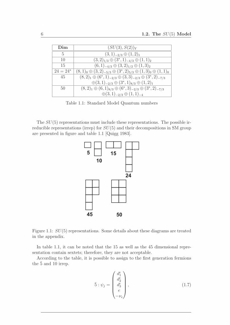
Table 1.1: Standard Model Quantum numbers

The SU(5) representations must include these representations. The possible ir-reducible representations (irrep) for SU(5) and their decompositions in SM groupare presented in figure and table 1.1 [Quigg 1983].

5

10

15

24

45 50

Figure 1.1: SU(5) representations. Some details about these diagrams are treatedin the appendix.

In table 1.1, it can be noted that the 15 as well as the 45 dimensional repre-sentation contain sextets; therefore, they are not acceptable.

According to the table, it is possible to assign to the first generation fermionsthe 5 and 10 irrep.

5 : ψj =

dc1

dc2

dc3

e−νe

, (1.7)


10 : ψjk =1√2

0 uc3 −uc

2 −u1 −d1

−uc3 0 uc

1 −u2 −d2

uc2 −uc

1 0 −u3 −d2

u1 u2 u3 0 −ec

d1 d2 d3 ec 0

(1.8)

In fact, there is no rule for using this assignation of particles but we can seethat these representations have the right quantum numbers as follows:

For 5 : dc(3∗,1)2/3

⊕ (e,−νe)(1,2∗)−1

For 10 : (u, d)(3,2)1/3⊕ uc

(3∗,1)−4/3⊕ ec

(1,1)2(1.9)

The next step is to check the gauge boson content. There are 24 bosons cor-responding to 24 elements of the SU(5) adjoint. The SM gauge bosons have thefollowing numbers:

(8, 1)0 ↔ Gluons,

(1, 3)0 ↔ W+µ ,W

−µ ,W

3µ ,

(1, 1)0 ↔ Aµ (1.10)

SU(5) contains the SM gauge bosons and extra gauge fields which are knownas leptoquarks since they induce interactions between quarks and leptons. Thequantum numbers of these new leptoquark gauge bosons are given by

(3, 2)−5/3 ↔ Xµ, Yµ,

(3∗, 2)5/3 ↔ Xµ, Yµ. (1.11)

According to the decomposition of the SU(5) adjoint, we can write the bosoncontent as follows:

V =1√2

GluonsX1 Y1

X2 Y2

X3 Y3

X1 X2 X3

Y1 Y2 Y3

W3√2

W+

W− −W3√2

+1√30B

−2 0 0 0 00 −2 0 0 00 0 −2 0 00 0 0 3 00 0 0 0 3

(1.12)

This decomposition corresponds to a group of generators. The generators havebeen chosen such that the first eight ones are the SU(3) generators, namely La

with a = 1, 2, ..., 8. The three following generators belong to SU(2): L8+i, wherei = 1, 2, 3. L12 is assigned to hypercharge. Then, the first twelve generators areplaced in these matrices:


La =

(

λa 00 0

)

(1.13)

L8+i =

(

0 00 τi

)

(1.14)

L12 =

(

C3I3×3 00 C2I2×2

)

(1.15)

C2 and C3 are two constants that will be determined below.The SU(N) generators are normalized according to [Cheng and Li 1984]:

Tr(LαLβ) = 2δαβ (1.16)

Tr(Lα) = 0. (1.17)

For the SU(3)C and SU(2)L generators these conditions are automatically satis-fied. For L12, we must determinate the constants according to the last conditions.From (1.17), C3 = −2

3C2 and from (1.16), 3C2

3 + 2C22 = 2, then it is possible to

find C2 =√

3/5 and C3 = −√

4/15. So, L12 is

L12 =

(

− 2√15I3×3 0

0 3√15I2×2

)

(1.18)

The hypercharge generator is proportional to generator L12, Y = CL12, andelectric charge is defined as Q = L11 + Y

2= L11 + 1

2CL12.

For the 5 irrep, Q = (1/3, 1/3, 1/3,−1, 0) or Q(ψi) = δijQj. This implies

Tr(Q2) =4

3= Tr(L2

11) +C2

4Tr(L2

12) =1

2(1 + C2) (1.19)

Then,

C2 =5

3(1.20)

With this value, hypercharge takes a definite and non arbitrary form

Y =

−23

0 0 0 00 −2

30 0 0

0 0 −23

0 00 0 0 1 00 0 0 0 1

(1.21)

As ψjk transforms as a tensor (2, 0), it has the same quantum numbers as ψjψk.Thus, the charge for 10 and 24 multiplets can be expressed as


Q(ψij) = Qi +Qj (1.22)

Q(ψij) = Qi −Qj

The gauge bosons are placed in a 24 dimensional representation, as follows

24 = (8, 1)⊕ (1, 3)⊕ (1, 1)⊕ (3, 2)⊕ (3∗, 2). (1.23)

The three first terms correspond to the SM gauge bosons which are 12. Thegenerators for the remaining 12 gauge boson field can be written in terms of thefollowing matrices:

A1 =

1 00 00 0

, A2 =

0 01 00 0

, A3 =

0 00 01 0

(1.24)

B1 =

0 10 00 0

, B2 =

0 00 10 0

, B3 =

0 00 01 1

,

and the resulting generators become

L11+2k =

(

03 Ak

ATk 02

)

(1.25)

L12+2k =

(

03 −iAk

iATk 02

)

L17+2k =

(

03 Bk

BTk 02

)

L18+2k =

(

03 −iBk

iBTk 02

)

k = 1, 2, 3.

Now, with this definition, the whole gauge boson set can be expressed as alinear combination of generator matrices:

Aµ =1

2

24∑

a=1

AaµLa (1.26)

And the new gauge bosons are defined as

X1

µ =A13

µ − iA14µ√

2, X

2

µ =A15

µ − iA16µ√

2, X

3

µ =A17

µ − iA18µ√

2

Y1

µ =A19

µ − iA20µ√

2, Y

2

µ =A21

µ − iA22µ√

2, Y

1

µ =A23

µ − iA24µ√

2(1.27)


Finally, as a consistency check, it must be proved that model is anomaly freeas it contains the SM which we already know is anomaly-free [Mohapatra 2002][Cheng and Li 1984]. The anomaly of any fermion representation is proportionalto the trace.

Tr(T a(R), T b(R)T c(R)) =1

2A(R)dabc (1.28)

with dabc totally symmetric and T a are the group generators in such a represen-tation.

Since expression (1.28) is generator independent, we can select T a = T b = T c =Q. Then,

A(5∗)

A(10)=

Tr(Q3(ψi))

Tr(Q3(ψij))

=3(1/3)3 + (−1)3

3(−2/3)3 + 3(2/3)3 + 3(−1/3)3 + 1= −1 (1.29)

thereforeA(5∗) + A(10) = 0 (1.30)

Thus the fermion representation that we have chosen is anomaly free.

1.2.2 Spontaneous symmetry breaking

When SU(5) is unbroken, all the fields are massless. The SU(5) fields acquiremass through the spontaneous breaking of the GUT gauge symmetry. The break-ing occurs at a scale larger thanMW scale in order to preserve the proton stability.Thus, MX ≫ MW . The phenomenon that provides masses for gauge bosons isknown as the Higgs mechanism. In this mechanism scalar fields develop a vacuumexpectation value (VEV). A standard description of this procedure can be foundin [Cheng and Li 1984] and [Li 1964].

The SSB in the SU(5) model occurs in two steps, namely

SU(5)Σ→ SU(3)C × SU(2)L × U(1)Y

Φ→ SU(3)C × U(1)Q (1.31)

The first step is induced by the VEV of a Higgs multiplet placed in the adjoint24 dimensional representation Σ. SU(5) is broken at a GUT scale around 1016

GeV. At this scale the SM bosons are still massless. The most general scalarpotential describing the interactions of Σ is

V (Σ) = −m21(Tr Σ2) + λ1(Tr Σ2)2 + λ2(Tr Σ4) (1.32)

The cubic term has been omitted to leave the potential invariant under Σ →−Σ. V(Σ) has an extremum at Σ = 〈Σ〉 with

〈Σ〉 = V

22

2−3

−3

(1.33)


where

V 2 =m2

1

(60λ1 + 14λ2)(1.34)

A normalisation factor 1/√

60 is absorbed in V .The field is shifted to define the new set of scalar fields:

Σ′ = Σ− 〈Σ〉 =

[Σ8]αβ − 2√

30Σ0

ΣX1ΣY1

ΣX2ΣY2

ΣX3ΣY3

ΣX1ΣX2

ΣX3

ΣY1ΣY2

ΣY3

[Σ3]rs − 3√

30Σ0

(1.35)

The mass spectrum of this scalars can be found by expressing Σ as a diagonal-ized matrix Σiδ

ij and evaluating

∂2V

∂Σi∂Σl 〈Σ〉(1.36)

Since Σ is in an adjoint representation, the covariant derivative can be written

DµΣ = ∂µΣ + ig5[Aµ,Σ] (1.37)

where g5 is the SU(5) coupling constant.

According to the redefinition of the Σ′ field,

DµΣ = ∂µΣ + ig5[Aµ,Σ′ + 〈Σ〉]

= DµΣ′ + ig5[Aµ, 〈Σ〉] (1.38)

Thus,|DµΣ|2 ⊃ g2

5|[Aµ, 〈Σ〉]|2 (1.39)

[Aµ, 〈Σ〉] =V√2

−5

X1 Y1

X2 Y2

X3 Y3

5

(

X1 X2 X3

Y1 Y2 Y3

)

(1.40)

The X and Y gauge bosons masses are determined by

g25|[Aµ, 〈Σ〉]|2 ∼ g2

5

25

2V (1.41)

such that MX = MY =√

25/2g5V .The SM gauge symmetry is spontaneously broken by the VEV of a scalar in a

5− dim representation. The scalar potential in this case is given by

Veff(φ) = −m2φ†φ+ λ3(φ†φ)2 (1.42)


and the VEV by

〈φ〉 =1√2

0000v

(1.43)

with v ≃ 246.2 GeV. The W± and Z0 gauge bosons acquire masses in a lowerscale; a representative fact is that V ≥ 1012v.SU(5) has a problem that is known as doublet triplet splitting. Each Higgs field

multiplet contains a doublet corresponding to the electroweak Higgs field, anda coloured triplet that acquires mass of the order of the GUT scale to avoid ashort proton lifetime. In minimal SU(5) this problem is solved using a fine tunedcancellation in the term λ1(H

ui H

djΣij +m′Hu

i Hdi).

1.2.3 SU(5) Lagrangian and gauge vertices

The kinetic term for the SU(5) Lagrangian is given by

L = i(ψ)ca(γ

µDµψ)ca + i(ψ)ab(γµDµψ)ab (1.44)

= (ψ)ca(iγ

µ∂µδab +

g5√2γµAa

µb)(ψc)b + (ψ)ab(iγ

µ∂µδbe +

g5√2γµAb

µe)(ψc)ae

The term involves the X and Y gauge bosons. For a single generation it canbe written as

LX,Y =ig5√

2Xµ,i(ǫijku

ckγ

µuj + diγµe) (1.45)

+ig5√

2Yµ,i(ǫijku

ckγ

µdj − uiγµec + dc

iγµν) + h.c

The Feynman diagrams which represent the above gauge intarcations are shownin the figures 1.2,1.3 and 1.4.

da

L

ua

L

W+

ub

Ua

Ga

b

nL

eL

W+

Figure 1.2: Feynman diagrams for the SM gauge boson interactions


e+

da

Xa

nc

da

Ya

e+

ua

Ya

Figure 1.3: Feynman diagrams for vector-like lepto-quark interactions

uc

g

da

Ya

uc

g

ub

Xa

Figure 1.4: Feynman diagrams for diquark interactions

The decays involving leptoquarks (V ) violate B-number and L-number. Thisis:

V → lL ucR B = −1/3 B − L = 2/3

V → qL dcR B = 2/3 B − L = 2/3 (1.46)

Then, B − L is conserved. This feature was in the past a motivation to GUTbariogenesis [Chen 2006], but it was found that generating the sufficient B asym-metry requires high reheating temperature.

1.2.4 Coupling constants and renormalization group

The SM makes predictions for energies below 1 TeV. At these energies interactionsare not unified, there are three unrelated coupling constants gs, g and g′ forSU(3)C , SU(2)L and U(1)Y respectively. In this theory there is no a explanationfor the different strengths of this couplings.

The idea of a Grand Unified Theory is that all interactions are described byone single coupling constant. The three gauge couplings of the SM arise afterthe SU(5) symmetry breaking. As X and Y acquire masses, the renormalisationgroup is decoupled into three subgroups.

In 1974, Georgi, Quinn and Weinberg [Georgi et al 1974] observed that the cou-pling constants behave in a scale-dependent way and vary according to the energyscale in such a way that they must be equal to the SU(5) coupling constant atsome energy scaleMU . In 1975, Appelquist and Carazone [Appelquist-Carazone 1975]


presented what is known as the decoupling theorem which states that if a gaugeinvariant (under G) Lagrangian field theory contains particles with two very dif-ferent mass scales (m ≪ M) and is described by a renormalizable Lagrangian,the behaviour of the light particles in the theory can be described completely bya renormalizable Lagrangian that involves only these particles.

Because of this theorem, gauge couplings are able to be described, at the SMscale, by the β-functions corresponding to SU(3)C , SU(2)L and U(1)Y withouttaking into account SU(5):

dgi

dt= βi(gi) ≡ bi

g3i

16π2(1.47)

with i = 1, 2, 3 and t =lnµ, µ is the energy scale.

The relation between the SM and the SU(5) gauge couplings can be obtainedby a direct comparison of the covariant derivatives:

Dµ = ∂µ + igs

8∑

α=1

Gαµ

λα

2+ ig

3∑

r=1

W rµ

τ r

2+ ig′Bµ

Y

2(1.48)

Dµ = ∂µ + ig5

24∑

a=1

Aaµ

La

2(1.49)

The definition of the coupling constants is determined by the normalization ofthe generators.

In SU(5), g5 = gs = g = g1 where g1 corresponds to the U(1) coupling at theSU(5) scale. Non-Abelian groups have fixed coupling; therefore, the comparisonbetween the two covariant derivatives is made on the Abelian part.

ig1L12A12

µ ≡ ig′Y Bµ (1.50)

As A12µ has been assigned to Bµ, from the definition of hypercharge and L12:

g1L12 = g′Y

g1

√

3

5= g′ (1.51)

And this can be used to compute the weak angle (or Weinberg angle) [Georgi et al 1974]:

sin2θW =g′2

g2 + g′2

=35g2

g2 + 35g2

=3

8(1.52)


Coming back to equation (1.47), for the SM we have (without Higgs bosoncontributions)

b1 =2

3Nf

b2 = −(

22

3− 2

3Nf

)

b3 = −(

11− 2

3Nf

)

(1.53)

Where Nf is the number of fermions. If we define αi = g2i /4π, we obtain

dαi

dt=

1

2πgidgi

dt(1.54)

and thereforedαi

dt= bi

α2i

2π(1.55)

With these equations and the boundary conditions α1(MX) = α2(MX) =α3(MX) = αU we can compute the values for αi at MW scale. In order to do

it, we recall that α3(MW ) = αs(MW ), α2(MW ) = αW (MW ), 35α1(MW ) = g′2(MW )

4π

and the first part of equation (1.52).Solving the equations, we get

1

αi(µ)=

1

αU

+bi2π

ln

(

MX

µ

)

(1.56)

From solutions for i = 1, 2 we can obtain

1

α2(µ)− 1

α1(µ)= − 1

2π

22

3ln

(

MX

µ

)

(1.57)

Inserting this result in the definition of the weak angle, it is straightforwardobtain

sin2θW ≈3

8− 55α(µ)

24πlnMX

µ(1.58)

We can note that for the limit µ = MX , we return to result in equation (1.52).This result is for the case in which we have not included the Higgs doublet. Whenit is include the coefficient 55

24πis replaced by 109

48π[Mohapatra 2002].

Now, we shall compute the value of the weak angle at the MW scale. We takeα−1(MW ) ≃ 128 and MX = 2.1 × 1014 × 1.5±1 Λ

0.16GeVwhere Λ is the QCD scale

parameter that denotes the scale at which the QCD interactions are strong. Aplausible value for such parameter is given in [Mackenzie et Lepage 1981]: Λ =160+100

−80 MeV. Then,


sin2θW = 0.214± 0.003± 0.0028 (1.59)

but from PDG data, the experimental value is sin2θW = 0.23152 ± 0.00014[PDG 2006].

Evidently, this result does not coincide with the obtained before, this is becausethe condition of unification of coupling constants at GUT scale is not true. Theinterpolation of experimental data has shown that SU(5) without supersymmetrydoes not unify the interactions at any scale. This can be seen in figure 1.5

Log (Q/1 GeV)10

2 4 6 8 10 12 14 16 18

60

50

40

30

20

10

0

a2

-1

a3

-1

a1

-1

Figure 1.5: Evolution of the α−1 functions

1.2.5 Proton decay

One of the most important features of the SU(5) model and any of GUT theoryis the prediction of proton decay which arises from a set of tree-level X-bosonexchange. The Lagrangian involved in these processes is given by

LX,Y =1√2g5(Xµ,α[ǫαβγuc

γγµuβ + dαγ

µe+ − eγµdcα]

+Yµ,α[ǫαβγucγµdβ + uαγµe+ − νeγ

µdcα] (1.60)

From the expression (1.60) it is possible to find a set of ∆B = 1 process. Someof these are shown in figure 1.6. The effective Lagrangian for these processes is

L∆B=1 =g25

2M2X

ǫαβγǫab(ucγγ

µqβa)(dcαγµlb + e+γµaαb), (1.61)

where Xa = (X,Y ), qa = (u, d) and la = (ν, e). It is noted that ∆(B − L) = 0is a symmetry of the effective Lagrangian. Then, SU(5) contains some tow-body


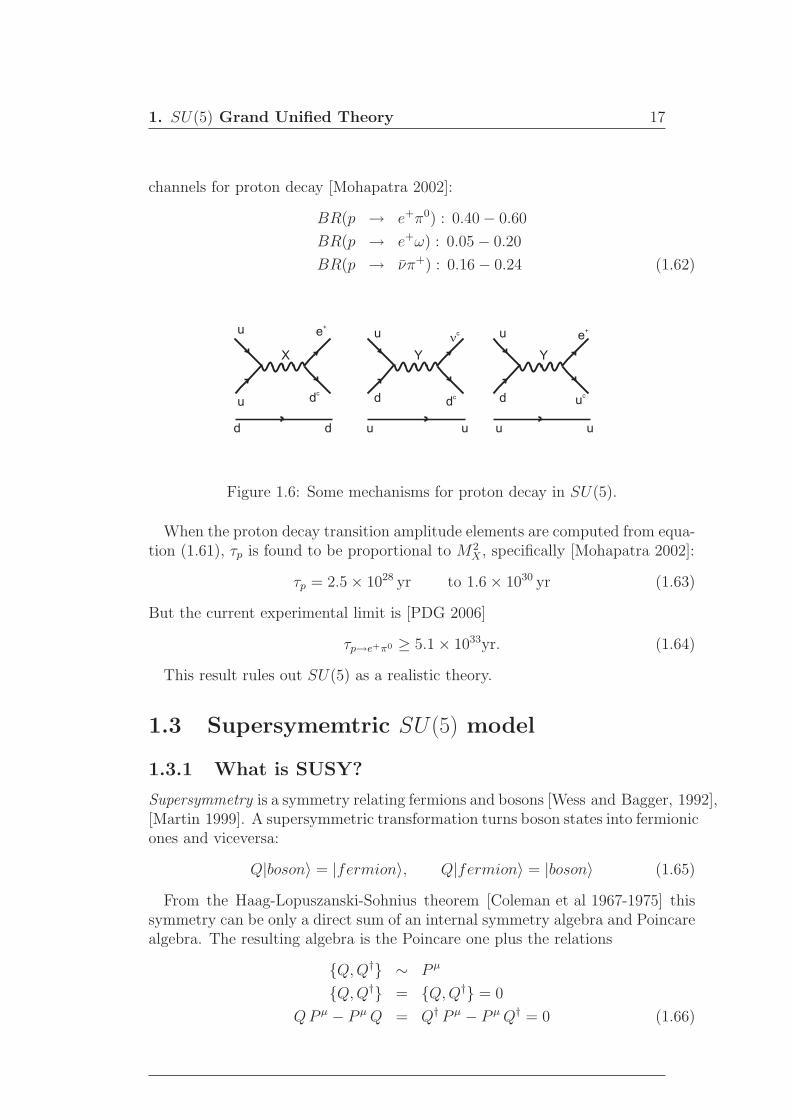
channels for proton decay [Mohapatra 2002]:

BR(p → e+π0) : 0.40− 0.60

BR(p → e+ω) : 0.05− 0.20

BR(p → νπ+) : 0.16− 0.24 (1.62)

u

u

u u

ucd

cdd d

c

nce

+

e+

X Y Y

d d u u uu

Figure 1.6: Some mechanisms for proton decay in SU(5).

When the proton decay transition amplitude elements are computed from equa-tion (1.61), τp is found to be proportional to M2

X , specifically [Mohapatra 2002]:

τp = 2.5× 1028 yr to 1.6× 1030 yr (1.63)

But the current experimental limit is [PDG 2006]

τp→e+π0 ≥ 5.1× 1033yr. (1.64)

This result rules out SU(5) as a realistic theory.

1.3 Supersymemtric SU(5) model

1.3.1 What is SUSY?

Supersymmetry is a symmetry relating fermions and bosons [Wess and Bagger, 1992],[Martin 1999]. A supersymmetric transformation turns boson states into fermionicones and viceversa:

Q|boson〉 = |fermion〉, Q|fermion〉 = |boson〉 (1.65)

From the Haag-Lopuszanski-Sohnius theorem [Coleman et al 1967-1975] thissymmetry can be only a direct sum of an internal symmetry algebra and Poincarealgebra. The resulting algebra is the Poincare one plus the relations

{Q,Q†} ∼ P µ

{Q,Q†} = {Q,Q†} = 0

QP µ − P µQ = Q† P µ − P µQ† = 0 (1.66)

18 1.3. Supersymemtric SU(5) model

Names spin 0 spin 1/2 (SU(3), S(2))Y

Q (uL dL) (uL dL) (3, 2)1/3

u u∗R u†R (3∗, 1)−4/3

d d∗R d†R (3∗, 1)2/3

L (ν eL) (ν eL) (1, 2)−1

e e∗R e†R (1, 1)2

Hu (H+u H0

u) (H+u H0

u) (1, 2)1

Hd (H0d H

+d ) (H0

d H−d ) (1, 2)−1

Table 1.2: The MSSM Supermultiplets

Names spin 1/2 spin 1 (SU(3), S(2))Y

gluino, gluon g g (8, 1)0

winos, W bosons W± W 0 W± W 0 (1, 3)0

bino, B boson B0 B0 (1, 1)0

Table 1.3: The MSSM Gauge supermultiplets

Q and Q† commute with the SM generators; therefore, the SM eigenstatesare also Q and Q† eigenstates. The irreducible representations of this algebraare called supermultiplets. Each supermultiplet contains both fermion and bosonstates. These are called superpartners. The names for the spin-0 partner of quarksand leptons are called squarks and sleptons respectively and are represented byadding a ∼ over the fermion symbol: νe, uR, eL, etc. In the Minimal Supersym-metric Standard Model (MSSM) there are two Higgs supermulfields (each withY = ±1) in order to avoid triangular gauge anomalies and because of the holo-morphy of the superpotential. On the other hand, the gauge bosons have theirsuperpartners called gauginos. The content of chiral and gauge supermultipletsof the MSSM is shown in tables 1.2 and 1.3.

One important fact about SUSY is that none of the spartners of the SM par-ticles has been discovered yet and SUSY is a softly broken symmetry.

1.3.2 SUSY SU(5)

To construct the supersymmetric extension of the SU(5) model, we need twoHiggs superfields Hu and Hd which belong to 5φu and 5φd representations. Weuse a 24-dimensional superfield Σ to break the SU(5) gauge symmetry.

The superpotential for the model is given by [Mohapatra 2002]

W = yuǫijklmψijψklH

um +ydψijψ

iHdj +xTr Σ2 +λ1(Hui H

djΣij +m′Hu

i Hdi) (1.67)

Since SUSY involves new fields, there will be new contributions to the β func-tion that will affect the evolution of the coupling constants. For supersymmetric


SU(N) the β function is given by [Martin 1999]

βi(gi) = b0ig3

i

16π2(1.68)

where b0i = −3N + Nf + NH . The changes in the contributions is caused bythe supersymmetric partners. The evolution for coupling constant within thiscontext is shown in figure 1.7. The new content of particles affects the evolutionof gauge coupling as well the GUT scale. The new unification scale is given by

MX,Susy ≃ 6× 1016 GeV (1.69)

.Then, we have that MX is larger and, therefore, the proton lifetime acquires a

new value: τp ≃ 1034 yr. Thus, this model is consistent with experimental data.

60

10

20

30

40

50

2 6 8 10 124 1614 180

Log (Q/1 GeV)10

a2

-1

a1

-1

a-1

a3

-1

Figure 1.7: Evolution of α−1 within the MSSM.

SUSY SU(5) still suffer the so-called the doublet triplet splitting problem thatwe have mentioned above.

20 1.3. Supersymemtric SU(5) model

Chapter 2

Horizontal symmetries and

Froggatt-Nielsen mechanism

“Physics should be beautiful.”

Sir F. Hoyle

2.1 The fermion mass hierarchy problem

An important fact from experimental data is that there is a large hierarchy amongthe particle masses belonging to different generations. That is mu ≪ mc ≪ mt.This is the fermion mass hierarchy problem: there is no explanation for neitherthis hierarchy nor the quark mixing pattern.

The most general Yukawa Lagrangian in the SM has the following form [Pich 1994]:

LY = ydjkQ

′LjΦd

′Rk + yu

jkQ′LjΦu

′Rk + yl

jkL′Φl′Rk (2.1)

where we are using the notation of equation (1.1) and Φ represents the Higgsfield. The indices run over the three generations and the prime indicates thatthese fields are written in the gauge interaction basis.

After the SSB this Lagrangian becomes

LY = d′LM′

dd′R + u′

LM′uu

′R + l′LM

′ll′R (2.2)

Here, the corresponding mass matrices are given by

(M′d)ij ≡ −yd

ijv/√

2, (M′u)ij ≡ −yu

ijv/√

2, (M′d)ij ≡ −yl

ijv/√

2 (2.3)

The diagonalization of these matrices yield the quark and charged lepton masses.M′

u is not an Hermitian matrix but M′uM′†

u do is. Then the latter can bediagonalized by an unitary matrix. The same occurs withM′†

uM′u. Let UL and

UR be two matrices such that they diagonalize the last two Hermitian matricesrespectively. Thus, the matrixM′

u is diagonalized as

ULM′uU †

R =Mu (2.4)

21

22 2.1. The fermion mass hierarchy problem

In the same way, there are two matrices DL and DR that diagonalizeM′d:

DLM′dD†

R =Md (2.5)

Now, inserting these matrices in the Lagrangian we obtain the Yukawa La-grangian in the with mass eigenstate basis.

LY = d′LD†

LDLM′dD†

RDRd′R + u′

LU †LULM′

uU †RURu′

R + h.c.

= dLMddR + uLMuuR + h.c.

= dMdd + uMuu (2.6)

where the mass eigenstates are defined

dL,R ≡ DL,Rd′L,R uL,R ≡ UL,Ru′

L,R (2.7)

The charged current Lagrangian of SM has the form

L =g

2√

2W †

µ[u′γµ(1− γ5)d′ + ν ′γµ(1− γ5)l

′] + h.c. (2.8)

Inserting the mass eigenstates, this Lagrangian becomes

L =g

2√

2W †

µ[uγµ(1− γ5)Vd + νγµ(1− γ5)l] + h.c. (2.9)

Here, V is a mixing matrix called the Cabibbo-Kobayashi-Maskawa (CKM)matrix and it is given by

V ≡ ULD†L (2.10)

We note that this matrix mixes any up-type quark with all down-type quarks.Also, it can be noted that there is no mixing among leptons, this is because inthe SM neutrinos are massless; so, it is always possible to rotate the neutrinofields in such a way that the charged lepton mass matrix remains diagonal.

The CKM matrix can be parametrised with three mixing angles and one phase,[PDG 2006] R(θ12)R(θ13, δ13)R(θ23):

V =

c12c13 s12c13 s13e−iδ13

−s12c23 − c12s23s13e−iδ13 c12c23 − s12s23s13e

−iδ13 s23c13s12c23 − c12s23s13e

−iδ13 −c12c23 − s12s23s13e−iδ13 c23c13

(2.11)

where cij ≡ cos(θij) and i, j are generation indexes. Experiments have shownthat s13 ≪ s23 ≪ s12.

Another parametrization, given by Wolfenstein, exhibit explicitly the mass hi-erarchy:

s12 = λ s23 = Aλ2 s13eiδ = Aλ3(ρ+ iη) (2.12)

2. Horizontal symmetries and FN mechanism 23

In this way, the CKM matrix takes the form

V =

1− λ2/2 λ Aλ3(ρ− iη)−λ 1− λ2/2 Aλ2

Aλ3(1− ρ− iη) A− λ2 1

(2.13)

Since this matrix is unitary, VijV∗jk = δik, a common unitary triangle arises

from VudV∗ub + VcdV

∗cb + VtdV

∗tb = 0. This relation, in terms of (ρ), η is used to

present measurements of CKM elements [PDG 2006].The SM quark masses at MZ scale take the following values [Aristizabal 2003],

[PDG 2006]:

mu = 2.33+0.42−0.45 MeV, mc = 677+56

−61 MeV, mt = 181± 13 GeV

md = 4.69+0.60−0.66 MeV, ms = 93.4+11.8

−13.0MeV, mb = 3.00± 11 GeV(2.14)

The relations among the masses of the different quark generations (atMZ scale)can be expressed in powers of λ = 0.22:

mu

mc

= 0.0034 ∼ λ3 md

ms

= 0.0521 ∼ λ2

mb

mt

= 0.0165 ∼ λ2 mc

mt

= 0.0037 ∼ λ3

ms

mb

= 0.0311 ∼ λ2 (2.15)

2.2 Horizontal symmetries

The fermion mass hierarchy can be explained through the Froggatt-Nielsen Mech-anism [Froggatt and Nielsen 1979]. According to this approach, a globalH sym-metry spontaneously broken by the VEV of an scalar singlet is responsible of theobserved fermion mass pattern.

Let H be a symmetry under which fields transforms as [Leurer et al 1992]:

Q→ LQ dR → RddR

uR → RuuR Φ→ PΦ (2.16)

In the mass basis:

uL → LuuL dL → LddL (2.17)

where Lu = ULLU †L and Ld = DLLD†

L such that Ld = V†LvV.The symmetry H is found to be broken: In fact, if H were unbroken, from

equation (2.1) and from the form in which fields transform, we would have:

LM′dRd =M′

d, LM′uRu =M′

u. (2.18)

24 2.2. Horizontal symmetries

Then, it is straightforward to show that

LM′dM′†

dL† =M′

dM′†d, LM′

uM′†uL

† =M′uM′†

u. (2.19)

Or in the mass basis[Ld,M2

d] = [Lu,M2u] = 0. (2.20)

This result says that if the symmetry were no broken there were degeneracyin the quark sector. Lu and Ld were forced to be diagonal, but because they arerelated by Ld = V†LvV they would have the same eigenvalues. If the eigenvalueswere different, i.e. there were no degeneracy, then all mixing angles were indeednull. So we can note that as there is no degeneracy in the quark sector and asthe three quark generations mix, H must be a broken symmetry.

As an explicit example, we take the SM and we consider an Abelian continuoussymmetry H = U(1)F at a very high energy scale. Once U(1)F is spontaneouslybroken by the VEV of a SM singlet scalar S, a set of effective operators are inducedby the integration of heavy fields of mass MF (much larger that electroweak SSBscale). These heavy fields couple to the SM fermions and Higgs boson as well.The breaking of U(1)F occurs at a scale ΛF ≃ 〈S〉. The hierarchy among fermionsis provided by the hierarchy among the effective operators which are suppressedby powers of the parameter λ = 〈S〉/MF [Duque 2006].

The Yukawa terms in the SM Lagrangian have the form

LYukawa = ydijQiφddj + yu

ijQiφuuj + h.c. (2.21)

At the scale in which H is an unbroken symmetry, for example, to produce upquarks terms of order 2, the Yukawa Lagrangian contains the Froggatt-Nielsenheavy fields R and T . To write it, we use the universality principle that supposesyd ≈ 1 and yu ≈ 1. Then, we have

LHexactY = QF (Q)φ0RF (R) + RF (R)S−1TF (T ) + TF (T )S−1uF (u) (2.22)

where the subindexes indicate the horizontal charge assignment. We assign thecharges F (φ) = F (φ) = 0 and F (S) = −1 and from this we can constrain thecharges of the other fields in such way that all the terms remain invariant underH.

F (Q) + F (R) = 0

F (R) + F (T ) = 1

F (T ) + F (u) = 1 (2.23)

A diagram for the horizontal interactions with two heavy fields is shown infigure 2.1.

According to the Feynman rules [Peskin 1995], the expression for the propaga-tors in the diagram 2.1 has the form

Qφi(γµp

µR +MF )

p2R +M2

F

Si(γµp

µT +MF )

p2T +M2

F

(2.24)

2. Horizontal symmetries and FN mechanism 25

u

Sf S

Q R R T T

Figure 2.1: SM horizontal symmetry diagram

i F(Q) F(u) F(d) F(L) F(e)1 3 5 3 1 62 2 2 2 1 63 0 0 2 1 1

Table 2.1: Charges for three fermion generations

The above expression produces the effective term once H is broken through〈S〉,

Leff = (〈S〉MF

)2Qφu+ h.c.. (2.25)

A general effective Lagrangian that includes the three fermion generations hasthe form

Leff = λnijQiφuj + λmijQiφdj + λsij Liφej + h.c. (2.26)

where nij = F (Qi) + F (uj),mij = F (Qi) + F (dj) and sij = F (Li) + F (ej) andthe mass matrices

Muij = vλF (Qi)+F (uj)

Mdij = vλF (Qi)+F (dj)

Mlij = vλF (Li)+F (ej) (2.27)

Now, we wonder if it is possible to find a set of charges that correctly fit themeasured masses and mixing angles.

We have found that with the charge assignment shown in the table 2.1 this canbe achieved.

It is straightforward to find the mass matrices

26 2.2. Horizontal symmetries

Mu = v

λ8 λ5 λ3

λ7 λ4 λ2

λ5 λ2 1

Md = vλ2

λ4 λ3 λ3

λ3 λ2 λ2

λ 1 1

Ml = vλ2

λ5 λ2 1λ5 λ2 1λ5 λ2 1

(2.28)

If we take λ ≈ 0.22, we can note that the quark matrices fit approximately tothe expected values for relations among the generations. Then, we can concludethat the Froggatt-Nielsen mechanism can provide approximately the hierarchyfor SM fermion masses. However, this method can only show the magnitudeorder of the entries but we can not compute the coefficients of each one. In thenext chapter we shall modify this method in order to properly compute thesecoefficients in a supersymmetric SU(5) extended with a horizontal symmetry.

Chapter 3

SU(5)× U(1)H Model

“Science is facts; just as houses are made of stones,

so is science made of facts; but a pile of stones is not a house

and a collection of facts is not necessarily science.”

Henri Poincare

In the last chapter we saw that the Froggatt-Nielsen mechanism can explainthe hierarchy fermion mass of the SM. In this chapter we will consider the SUSYSU(5) × U(1)H model. This model has been previously studied in references[Aristizabal 2003], [Duque 2006] and [Nardi et al 2007].

In this model, a horizontal Abelian flavor symmetry unbroken above the energyscale at which SU(5) is still an exact symmetry is implemented. Recently, Chenet al. have studied some features of such a symmetry in SU(5) [Chen 2008]. TheAbelian flavor symmetry, in that case, was broken through the VEV of a SU(5)scalar singlet as the one discussed in the last chapter. As a result, they arrivedat the mass hierarchy structure but without specifying coefficients of the entriesin the mixing matrix. Our goal is to get these coefficients by using a H-chargedSU(5) adjoint representation to break the Abelian symmetry. This idea wasproposed by Enrico Nardi and Diego Aristizabal from Universidad de Antioquia[Nardi et al 2007], [Aristizabal and Nardi 2004]. The main motivation for this isfound in the Georgi-Jarlskog’s article [Georgi and Jarlskog 1979]. They used a 45Higgs representation field in order to explain the difference in the lepton-quarkmass ratios for the three fermion generations.

3.1 The mass hierarchy at GUT scale

In 2007, Ross and Serna have given the mass structure for fermions at GUTscale [Ross-Serna 2007]. They took as starting point the values of fermion massesat a low energy scale and used the RG equations for different choices of tanβ(tanβ = 〈H0

u〉 / 〈Hod〉). The ratios in which we are concerned are

27

28 3.2. H-charge assignments Constraints

mu

mc

≈ 0.0027(6)mc

mt

≈ 0.0025(2)

md

ms

≈ 0.051(7)ms

mb

≈ 0.014(4)

me

mµ

≈ 0.0048(2)mµ

mτ

= 0.059(2). (3.1)

This is the GUT version of equation (2.15).We can express this structure using a parameter ǫ = 1

25≈ λ2.

mu : mc : mt = ǫ4 : ǫ2 : 1 md : ms : mb = ǫ3 : ǫ2 : ǫ (3.2)

The numerical VCKM at the GUT scale is given by [Fusaoka-Koide 1997]

V (MX) =

0.9754 0.2205 −0.0026−0.2203 0.9749 0.03180.0075 0.0311 0.9995

(3.3)

3.2 H-charge assignments Constraints

3.2.1 Anomaly cancellation

We must ensure that our model is anomaly free in what regards the horizontalcharge. This condition is expressed as

A =3∑

i=1

(H(5i) + 3H(10i)) +H(5φd) +H(5φu) = 0

=3∑

i=1

(fi + 3ti) + fd + fu = 0 (3.4)

where H(5i) = fi, H(10i) = ti and fd, fu are the H-charge for the Higgs fields[Nardi et al 2007].

This condition can be redefined by a set of shifts in the charges

fi → fi + a

ti → ti + b

fd → fd − (a+ b)

fu → fu − 2b (3.5)

such that the new anomaly term is

A′ = A+ 2(a+ 3b) (3.6)

The model requires the invariance of the term Mφφdφu under H. Then, a+3b =

0 and we have the following constraint:

b = −1

3a (3.7)

3. SU(5)× U(1)H Model 29

51 52 53 101 102 103

(1) 1 1 1 2 1 0(2) -1 -3 -1 -2 1 0(3) -5 1 1 2 1 0(4) 5 -3 -1 -2 1 0(5) 1 -3 1 2 1 0(6) -1 1 -1 -2 1 0(7) -5 -3 1 2 1 0(8) 5 1 -1 -2 1 0(9) 1 3 -1 2 -1 0(10) -1 -1 1 -2 -1 0(11) -5 3 -1 2 -1 0(12) 5 -1 1 -2 -1 0(13) 1 -1 -1 2 -1 0(14) -1 3 1 -2 -1 0(15) -5 -1 -1 2 -1 0(16) 5 3 1 -2 -1 0

Table 3.1: Possible H charge assignments

3.2.2 Charge assignments

From equation (3.2) and according to the idea of the FN mechanism, the hori-zontal charges for quarks must follow the equations

|101 + 101 + 5φu | = 4 |51 + 101 + 5φd | = 3

|102 + 102 + 5φu | = 2 |52 + 102 + 5φd | = 2

|103 + 103 + 5φu | = 0 |53 + 103 + 5φd | = 1 (3.8)

In addition, the term m′HdHu in the superpotential (1.67) must be invariant.This leads to the condition

fd + fu = 0 (3.9)

Then, from equations (3.8), (3.4) and (3.9) we have a set of linear equations.We obtained the set of solutions by choosing the charges to obey the equation

(3.8) and fd = fu = 0. For example, from |53 + 103 + 5φd | = 1 and |103 + 103 +5φu | = 0 it follows that t3 must be 0, and for f3 we have only two possibilities:f3 = ±1. After an iterative procedure for each pair of equations we find allpossible combinations. The results are shown in table 3.1.

We can discard eight solutions that have the same charges for two equal rep-resentations since they generate two rows proportional between them. Later, wediscard six solutions that generates entries of order 0 in the down-type quarkmatrix. Then we have two solutions, one of them does not satisfy the anomalycancellation. So we have an unique solution which corresponds to solution (11).

30 3.2. H-charge assignments Constraints

f1 f2 f3 t1 t2 t3 fu

-4 4 0 5/3 -4/3 -1/3 2/3

Table 3.2: Best H charge assignments for fermions in SU(5)× U(1)

We can make a shift such that b = −1/3 and in this case the new set of chargesis given in table 3.2. We make such a shift in order to avoid invariant terms ofthe type λ′ψijψiψj which can spoil proton stability. With this charge selection,the suppression factors in the effective Lagrangian can be written as:

ydij = Y d

ijǫfi+tj+fd , yu

ij = Y uij ǫ

ti+tj+fd . (3.10)

The charge assignment in table 3.2 generates the matrices for up and downtype quarks given in equation (3.11), where we assume Y d,u

ij to be of order unity.

M′u ∼

ǫ4 ǫ1 ǫ2

ǫ1 ǫ2 ǫ1

ǫ2 ǫ1 1

M′d ∼

ǫ3 ǫ6 ǫ5

ǫ5 ǫ2 ǫ3

ǫ1 ǫ2 ǫ1

(3.11)

3.2.3 Forbidden representations

In the matrices shown in equation (3.11) we note that the entriesMu12 andMu

21

are not very suppressed and, therefore, they affect the determinant of the matrix.This problem can be corrected by forbidding the representations involved in theeffective Lagrangian of order one.

The two possible diagrams at order one are shown in figure 3.1

S5f

RR 10

S 5f

RR 101010

Figure 3.1: Diagrams at order one

For the first diagram, the Lagrangian is

L = 10−4/35φu

2/3R2/3 +R−2/3Σ−1105/3. (3.12)

Where the subindexes indicate the horizontal charge assignment.We will find the representations valid for R.We know that 10⊗5 = 10⊕40 and 10⊗24 = 10⊕15⊕ 40. Then, we can assign

to R a representation 10 or 40. Thus, the representations 10−2/3 and 40−2/3 areforbidden.

3. SU(5)× U(1)H Model 31

On the other hand, the Lagrangian for the second diagram is

L = 10−4/3Σ−1R7/3 +R−7/35φu

2/3105/3. (3.13)

And, in this case, the representations 10−7/3 and 40−7/3 must be forbidden.

In conclusion, we must ignore the following representations:

10−2/3, 40−2/3

10−7/3, 40−7/3. (3.14)

And the new mass matrixM′u has the following structure

M′u ∼

ǫ4 ǫ2 ǫ2

ǫ2 ǫ2 ǫ1

ǫ2 ǫ1 1

(3.15)

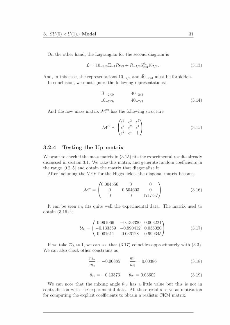
3.2.4 Testing the Up matrix

We want to check if the mass matrix in (3.15) fits the experimental results alreadydiscussed in section 3.1. We take this matrix and generate random coefficients inthe range [0.2, 5] and obtain the matrix that diagonalize it.

After including the VEV for the Higgs fields, the diagonal matrix becomes

Mu =

0.004556 0 00 0.504603 00 0 171.737

(3.16)

It can be seen mt fits quite well the experimental data. The matrix used toobtain (3.16) is

UL =

0.991066 −0.133330 0.003221−0.133359 −0.990412 0.0360200.001611 0.036128 0.999345

(3.17)

If we take DL ≈ 1, we can see that (3.17) coincides approximately with (3.3).We can also check other constrains as

mu

mc

= −0.00885mc

mt

= 0.00386 (3.18)

θ12 = −0.13373 θ23 = 0.03602 (3.19)

We can note that the mixing angle θ12 has a little value but this is not incontradiction with the experimental data. All these results serve as motivationfor computing the explicit coefficients to obtain a realistic CKM matrix.

32 3.3. Product of representations

Product Irreducible representations

5⊗ 5 1⊕ 2410⊗ 5 10⊕ 4010⊗ 10 1⊕ 24⊕ 7510⊗ 15 45⊕ ¯10515⊗ 5 35⊕ 4010⊗ 5 5⊕ 4515⊗ 5 5⊕ 7015⊗ 15 1⊕ 24⊕ 20040⊗ 5 45⊕ 50⊕ ¯10540⊗ 5 10⊕ 15⊕ 17545⊗ 5 10⊕ 40⊕ ¯17570⊗ 5 15⊕ ¯160⊕ 17524⊗ 5 5⊕ 45⊕ 7024⊗ 10 10⊕ 15⊕ 40⊕ 17524⊗ 15 10⊕ 15⊕ 160⊕ 17524⊗ 40 10⊕ 35⊕ 40⊕ 40⊕ ¯175⊕ ¯210⊕ 45024⊗ 45 45⊕ 45⊕ 5⊕ 50⊕ 70⊕ ¯105⊕ 280⊕ ¯48024⊗ 70 70⊕ 70⊕ 5⊕ 45⊕ 70⊕ ¯105⊕ 280⊕ 280⊕ ¯450⊕ ¯480

Table 3.3: Reduction of products of representations

3.3 Product of representations

Before going to the explicit calculation of some propagators, we present in table3.3 a kind of dictionary of the main reductions of the product of representations ofSU(5). Details about how to get these reductions can be found in the appendix.

3.4 The effective operators

Once we have the mass structure, the next step is to obtain the explicit coefficientsthrough a symmetry breaking using a H-charged adjoint representation. Theheavy fields are integrated out and the suppression term is given by powers ofǫ = 〈V 〉/MF , where 〈V 〉 is the VEV of the adjoint representation.

3.4.1 Computing the effective operators

Quantum field theory gives us the basic tools to compute the diagrams for thehorizontal interactions. We use the functional quantization for fermion fields[Pokorski 2000].

3. SU(5)× U(1)H Model 33

The generating functional of the Green’s function is given by the path integral

W [η, η] = N

∫

DΨDΨ exp[i(S[Ψ, Ψ] +

∫

d4x η(x)Ψ(x) + Ψ(x)η(x))]. (3.20)

Where N−1 = W [0, 0] and η , η are Grassmann fields. And the Feynman propa-gator is given by

SF (x− y) = 〈0|TΨ(x)Ψ(y)|0〉 = (i)−2 δ

δη(x)W [η, η]

←−δ

δη(x)|η=η=0. (3.21)

Propagator for the dimension 5 representation

The simplest propagator for the heavy fields, R and R, is the corresponding tothe 5 dimensional representation. For this one, we have the diagram 3.2. Thegenerating functional is given by

W [η, η] = N−1

∫

DRDR exp

[

− i

∫

d4xL0 +

∫

d4x(Raηa + ηcR

c)

]

(3.22)

Now, we have that the propagator [5]bd has the expression

[5bd] = (i)−2 δ

δηb

W [η, η]

←−δ

δηd

= iδ

δηb

∫

DRDR exp

[

− i

∫

d4xL0 +

∫

d4x(Raηa + ηcR

c)

]

(−Rmδmd )

= −∫

DRDR exp

[

−i∫

d4xL0 +

∫

d4x(Raηa + ηcR

c)

]

(RaRcδa

dδbc)η=η=0.(3.23)

We uses the theorem for functional determinants [Pokorski 2000]∫

DRDR exp

[

−i∫

d4xL0 +

∫

d4x(Raηa + ηcR

c)

]

(RdRb) =

(

1

6p−M + iǫ

)

δbd

(3.24)Then, the propagator takes the form

[5bd] = −

(

1

6p−M + iǫ

)

δbd (3.25)

Then, the effective propagator, when we have p≪M , for a 5 representation isgiven by

5b5d →1

Mδbd (3.26)

Now, we can compute the effective operator corresponding to the diagram 3.2and with Lagrangian

L = 5lΣlbR

b + Rd5φde 10de (3.27)

The effective Lagrangian that we obtain is

Leff = 5lΣlb([5]bd)5

φde 10de

=1

M5lΣ

ld5

φde 10de (3.28)

34 3.4. The effective operators

S 5f

5 R R 10

Figure 3.2: Horizontal symmetry for a 5 dimensional representation diagram

Propagators for the dimension 50(r) and 45 representations

Now, we shall obtain the effective propagator for the fields in a reducible repre-sentation 50ab

c . For this case, the generating functional is

W [η, η] =1

2

∫

DRDR exp

[

− i

∫

d4xL0 +

∫

d4x(Rpqrη

qrp + ηi

jkRjki )

]

. (3.29)

We take the equation (3.21) to write the propagator as:

[Rabc R

nlm] =

δ

δηcab

W [η, η]

←−δ

δηlmn

(3.30)

And then

[Rabc R

nlm] = (i)−2 δ

δηcab

1

2

∫

DRDR exp

[

− i

∫

d4xL0 +

∫

d4x(Rpqrη

qrp + ηi

jkRjki )

]

×(− i Rpqrδ

np (δq

l δrm − δq

mδrl ))

=1

2

∫

DRDR exp

[

− i

∫

d4xL0 +

∫

d4x(Rpqrη

qrp + ηi

jkRjki )

]

×(RpqrR

jki (δn

p (δql δ

rm − δq

mδrl )δ

ij(δ

aj δ

bk − δa

kδbj)) (3.31)

From QFT (see equation (3.24)),∫

DRDR exp[− i

∫

d4xL0 +

∫

d4x(Rpqrη

qrp + ηi

jkRjki )](Rp

qrRjki )

=1

6p−M + iǫδpi (δ

jqδ

kr − δj

rδkq ) (3.32)

Then, by replacing the above expression in equation (3.31) we obtain

[Rabc R

nlm] =

4

2(

1

6p−M + iǫ)(δn

c δal δ

bm − δn

c δamδ

bl )

= 21

6p−M + iǫδnc (δa

l δbm − δa

mδbl ). (3.33)

3. SU(5)× U(1)H Model 35

The effective operator for 50(r) becomes

[Rabc R

nlm]→ −2

1

Mδnc (δa

l δbm − δa

mδbl ) (3.34)

The 50(r) can be reduced to 5⊕ 45. Where 5a = Rjaj . Then, we can extract the

part of 50(r) corresponding to 5 to guarantee 45aba = 0. So,

45nlm = 50n

lm − (50bbmδ

nl + 50b

lbδnm). (3.35)

The final result is the whole effective propagator for the 45 representation:

[45abc 45

nlm]→ 1

2M{δa

c (δbl δ

nm−δb

mδnl )−δb

c(δal δ

nm−δa

mδnl )+4δn

c (δal δ

bm−δa

mδbl )} (3.36)

3.4.2 Some effective operators

Here we present some effective operators that will be useful to the specific coef-ficients of the mass matrices.

5a5b →1

Mδab . (3.37)

10ab10lm → 1

M(δa

l δbm − δa

mδbl ). (3.38)

15ab15lm → 1

M(δa

l δbm + δa

mδbl ). (3.39)

25(r)ab25(r)lm → 2

Mδal δ

bm. (3.40)

45abc 45

nlm → − 1

2M{δa

c (δbl δ

nm − δb

mδnl )− δb

c(δal δ

nm − δa

mδnl ) +

+4δnc (δa

l δbm − δa

mδbl )}. (3.41)

40abc40lmn → 3

Mδcn(δa

l δbm − δa

mδbl )−

1

2Mǫijabcǫijlmn (3.42)

50(r)abc 50

(r)nlm → − 2

Mδnc (δa

l δbm − δa

mδbl ). (3.43)

70abc 70

nlm → −1

2{δa

c (δbl δ

nm + δb

mδnl ) + δb

c(δal δ

nm + δa

mδnl )

−6δnc (δa

l δbm + δa

mδbl ))}. (3.44)

3.4.3 Explicit calculation in an anomalous model

There is a charge assignment that satisfies (3.8) and (3.9) but not (3.4). Thiskind of model is called anomalous. The anomaly can be cacelled by using theGreen-Schwarz mechanism [Green and Schwarz 1984]. In this section, we shallcompute the specific coefficients for the matrices built with the charges shown intable 3.4. The resulting matrices are given by (3.45).


f1 f2 f3 t1 t2 t3 fu

-4 -2 2 5/3 2/3 -1/3 2/3

Table 3.4: Anomalous charges assignment for fermions in SU(5)× U(1)

Mu ∼

ǫ4 ǫ3 ǫ2

ǫ3 ǫ2 ǫ1

ǫ2 ǫ1 1

Md ∼

ǫ3 ǫ4 ǫ5

ǫ1 ǫ2 ǫ3

ǫ3 ǫ2 ǫ1

(3.45)

It can be noted that Md has also problems in the entry 21. This implies thatwe must forbid some representations in order to reduce the order of magnitudedown to ǫ3. Using the same procedure as above, we find that the forbiddenrepresentations are:

158/3, 51, 451, 108/3, 155/3, 452 (3.46)

The Md33 entry

We start our specific calculation with the lowest order in the matrix for down-typequarks. There are two possible Lagrangian for this entry, namely

L = 5ΣR + R5φd10 (3.47)

L = 55φdR + RΣ10 (3.48)

For the Lagrangian (3.47) we have that the possible representations for R are 5and 45. To find the representations, we use the same arguments as for (3.12) andthe table 3.3. We can compose a 50(r) representation with those representations.Then, the Lagrangian can be written as

L50 = 5aΣcb50ab

c + 50nlm5φd

n 10lm (3.49)

The following step is to introduce the effective propagator (3.43) and use theΣ VEV 〈Σa

b〉 = 〈Va〉δab , given in (1.33).

L50eff = 5aΣ

cb[50ab

c 50nlm]5φd

n 10lm

= − 2

M5aΣ

cb(δ

nc (δa

l δbm − δa

mδbl ))5

φdn 10lm

= − 2

M5aVcδ

cb(δ

nc (δa

l δbm − δa

mδbl ))5

φdn 10lm

= − 2

M5aV5(δ

al δ

5m − δa

mδ5l ))〈5φd〉10lm

= − 2

M(−3V )(5a〈5φd〉10a5 − 5a〈5φd〉105a)

=12V

M(5a〈5φd〉10a5)

= 12V

M〈5φd〉(bcibi + τ cτ) (3.50)

3. SU(5)× U(1)H Model 37

Where i = 1, 2, 3.Now, for the Lagrangian (3.48) the possible representations for R are 10 and

15. So, we use a 25(r).

L25 = 5a5φd

b Rab + RlmΣm

n 10ln (3.51)

The effective Lagrangian becomes

L25 = 5a5φd

b [RabRlm]Σmn 10ln

= 5a5φd

b (2

Mδal δ

bm)Σm

n 10ln

=2

M5l〈5φd〉δ5

bVbδbn10ln

=2

M5l〈5φd〉(−3V )10l5

= −6V

M5l〈5φd〉10l5

= −6V

M〈5φd〉(bcibi + τ cτ) (3.52)

Then, from (3.50) and (3.52) the coefficient for the 33 entry of the down-matrixis

O(ǫ)→ 12− 6 = 6 (3.53)

The Md22 entry

The entry 22 of the down matrix has order 2. This implies that we have to intro-duce two heavy fields R and F . There are three possible Lagrangian densities.

L = 5 5φd R + RΣF + F Σ 10 (3.54)

L = 5 ΣR + R 5φd F + F Σ 10 (3.55)

L = 5 ΣR + RΣF + F 5φd 10 (3.56)

When we take into account the forbidden representation constraints we obtainthat only two effective operators contribute to the coefficient:

Leff 1 = 5 Σ [70] Σ [5] 5φd 10

Leff 2 = 5 Σ [70] Σ [45] 5φd 10 (3.57)

We shall compute here the Leff 1. The Lagrangian is written as

L = 5aΣcb70ab

c + 70nlmΣl

n5m + 5p5φdq 10pq (3.58)

The next step is to include the effective operators for the 5 and 70 representa-tions.


Leff 1 = 5aΣcb[

6

Mδnc (δa

l δbm − δa

mδbl )−

1

M(δa

c (δbl δ

nm + δb

mδnl ) + δb

c(δal δ

nm + δa

mδnl )]

×Σln(

1

Mδmp )5φd

q 10pq

=1

M2(6 5l〈Σn〉δn

m〈Σl〉δln5φd

l 10mq + 6 5m〈Σn〉δnl 〈Σl〉δl

n5φdq 10mq

−5m〈Σc〉δcl 〈Σl〉δl

m5φdq 10mq

=V 2

M2〈5φd〉(200 5i 10i5 + 225 54 1045) (3.59)

Using the same procedure, the contribution for leptons and quarks, from thesecond Lagrangian, are respectively 225 and −200.

The Mu23 entry

The entry Mu33 ∼ ǫ involves two possible diagrams as shown in figure 3.1. This

implies four effective operators:

Leff 1 = 10Σ[10]5φu10

Leff 2 = 10Σ[40]5φu10

Leff 3 = 105φu [10]Σ10

Leff 4 = 105φu [40]Σ10 (3.60)

We shall write the calculation for Leff 4. The rest of results are shown in table3.13.

We have that the exact Lagrangian is given

L = 10lm5φu n40lmn + 40abeΣdf10efǫabcde (3.61)

Then, we introduce the effective propagator (3.42).

Leff = 10lm5φu n[3

Mδnc (δa

l δbm − δa

mδbl )−

1

2Mǫijabcǫijlmn]Σd

f10ef

=6

M10ab5φu cΣd

f10efǫabcde

− 1

2M10lm5φu nΣd

fǫijabcǫijlmnǫabcde

=6

M10ab5φu cΣd

f10efǫabcde

− 1

2M10lm5φu nΣd

f (δidδ

je − δi

eδjd)ǫijlmn

=6

M10ab5φu cΣd

f10efǫabcde −1

M10lm5φu nΣd

fǫdelmn

=5

M10ab5φu cΣd

f10efǫabcde

3. SU(5)× U(1)H Model 39

Let us take 10411023, 〈Σab〉 = 〈Va〉δa

b and 〈5φu c〉 = 〈5φu〉δc5.

Leff =2× 5

M〈5φu〉(10411023〈Vd〉δd

3ǫd2415 + 10411032〈Vd〉δd2ǫd3415

+10321041〈Vd〉δd1ǫd4325 + 10321014〈Vd〉δd

4ǫd1325)

= 30V

M〈5φu〉10411023 (3.62)

Then, the contribution from this effective operator is 30.

3.5 Results for fermion matrices

We present the coefficients obtained for some entries of up, down and chargedlepton mass matrices.

The contributions from allowed effective operators for each entry in the matricesfor down quarks and leptons are presented in tables 3.5 to 3.12.

For the entry 22 at order ǫ2 (table 3.9), the quark coefficient vanishes, thenwe must look for contributions at order ǫ3. These contributions are given intable 3.10. These coefficients and those involving the 40 representation havebeen taken from [Nardi et al 2007]. We have redefined ǫ as ǫ/

√60 because of the

normalization factor of Σ . The arrows ↑ and ↓ indicate the calculation derivedform the two different possible contractions of the representation.

We also present some partial results that we have obtained with the up typequark matrix. This calculation is a work in progress,we show, in tables 3.11 to3.15, some of the contributions computed up to now.

The matrix obtained for down quarks is given by

M′d ∼

1110ǫ3 5139ǫ4 106007ǫ5

−1070ǫ3 −1000ǫ3 −2050ǫ3

−299ǫ3 232ǫ2 6ǫ1

(3.63)

We have used a random number for entries 12 and 13 since they are highlysuppressed. The matrix D†

L (see equation (2.5)) obtained for such a matrix is

D†L =

0.98500 −0.17249 0.00191−0.17249 −0.98501 0.00138−0.00164 0.00169 0.99999

(3.64)

And the diagonal matrix for quark masses is

Md =

0.00479 0 00 0.13315 00 0 5.81271

(3.65)

The mass ratios obtained are

md

ms

= 0.0359ms

mb

= 0.0229 (3.66)

40 3.5. Results for fermion matrices

Effective operator Lepton Down

5Σ[50(r)]5φd10 12 12

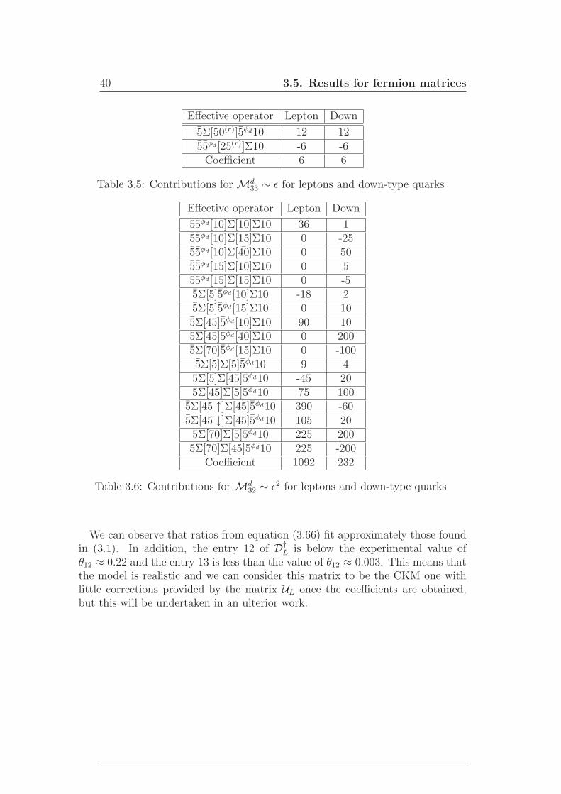
55φd [25(r)]Σ10 -6 -6Coefficient 6 6

Table 3.5: Contributions forMd33 ∼ ǫ for leptons and down-type quarks


55φd [10]Σ[10]Σ10 36 155φd [10]Σ[15]Σ10 0 -2555φd [10]Σ[40]Σ10 0 5055φd [15]Σ[10]Σ10 0 555φd [15]Σ[15]Σ10 0 -55Σ[5]5φd [10]Σ10 -18 25Σ[5]5φd [15]Σ10 0 105Σ[45]5φd [10]Σ10 90 105Σ[45]5φd [40]Σ10 0 2005Σ[70]5φd [15]Σ10 0 -1005Σ[5]Σ[5]5φd10 9 45Σ[5]Σ[45]5φd10 -45 205Σ[45]Σ[5]5φd10 75 100

5Σ[45 ↑]Σ[45]5φd10 390 -605Σ[45 ↓]Σ[45]5φd10 105 205Σ[70]Σ[5]5φd10 225 2005Σ[70]Σ[45]5φd10 225 -200

Coefficient 1092 232

Table 3.6: Contributions forMd32 ∼ ǫ2 for leptons and down-type quarks

We can observe that ratios from equation (3.66) fit approximately those foundin (3.1). In addition, the entry 12 of D†

L is below the experimental value ofθ12 ≈ 0.22 and the entry 13 is less than the value of θ12 ≈ 0.003. This means thatthe model is realistic and we can consider this matrix to be the CKM one withlittle corrections provided by the matrix UL once the coefficients are obtained,but this will be undertaken in an ulterior work.

3. SU(5)× U(1)H Model 41


55φd [10]Σ[10]Σ[10]Σ10 0 155φd [10]Σ[10]Σ[15]Σ10 0 -25

55φd [25(r)]Σ[10]Σ[40]Σ10 0 -30055φd [10]Σ[15]Σ[10]Σ10 0 -2555φd [10]Σ[15]Σ[15]Σ10 0 2555φd [10]Σ[40]Σ[10]Σ10 -54 -5

55φd [10]Σ[40 ↑]Σ[40]Σ10 0 -20055φd [10]Σ[40 ↓]Σ[40]Σ10 0 35055φd [15]Σ[10]Σ[10]Σ10 0 555φd [15]Σ[10]Σ[15]Σ10 0 -12555φd [15]Σ[15]Σ[10]Σ10 0 -555φd [15]Σ[15]Σ[15]Σ10 0 5

Coefficient -54 -299

Table 3.7: Contributions forMd31 ∼ ǫ3 for charged leptons and down type quarks


5Σ1[70]Σ1[5]5φd [10]Σ−110 1350 2005Σ1[70]Σ1[5]5φd [15]Σ−110 0 10005Σ1[70]Σ1[45]5φd [10]Σ−110 1350 -2005Σ1[70]Σ1[45]5φd [40]Σ−110 0 -40005Σ1[70]Σ1[70]5φd [15]Σ−110 0 -4005Σ1[70]Σ1[70]5φd [15]Σ−110 0 8005Σ−1[5]5φd [10]Σ1[40]Σ110 0 -1005Σ−1[45]5φd [10]Σ1[40]Σ110 0 1200

5Σ−1[45 ↑]5φd [40]Σ1[40]Σ110 -1248 10445Σ−1[45 ↓]5φd [40]Σ1[40]Σ110 456 -614

Coefficient 1908 -1070

Table 3.8: Contributions forMd21 ∼ ǫ3 for leptons and down type quarks


5Σ[70]Σ[5]5φd10 225 2005Σ[70]Σ[45]5φd10 225 -200

Coefficient 500 0




5Σ1[70 ↑]Σ0[70]Σ1[45]5φd10 -4725 -8005Σ1[70 ↓]Σ0[70]Σ1[45]5φd10 -675 16005Σ0[70 ↑]Σ1[70]Σ1[45]5φd10 -4725 -8005Σ0[70 ↓]Σ1[70]Σ1[45]5φd10 -675 16005Σ0[70 ↑]Σ1[70]5φd [15]Σ110 0 -4005Σ0[70 ↓]Σ1[70]5φd [15]Σ110 0 8005Σ0[70]Σ1[5]5φd [10]Σ110 1350 2005Σ0[70]Σ1[5]5φd [15]Σ110 0 10005Σ0[70]Σ1[45]5φd [10]Σ110 1350 -2005Σ0[70]Σ1[45]5φd [40]Σ110 0 -4000




5Σ[70]Σ[5]5φd [10]Σ10 1350 2005Σ[70]Σ[5]5φd [15]Σ10 0 10005Σ[70]Σ[45]5φd [10]Σ10 1350 -2005Σ[70]Σ[45]5φd [15]Σ10 0 -505Σ[70]Σ[5]Σ[5]5φd10 -675 4005Σ[70]Σ[5]Σ[45]5φd10 1125 10005Σ[70]Σ[45]Σ[5]5φd10 1125 -2000

5Σ[70]Σ[45 ↑]Σ[45]5φd10 4275 12005Σ[70]Σ[45 ↓]Σ[45]5φd10 1575 -4005Σ[70 ↑]Σ[70]Σ[5]5φd10 -4725 8005Σ[70 ↓]Σ[70]Σ[5]5φd10 -675 -16005Σ[70 ↑]Σ[70]Σ[45]5φd10 -4725 -8005Σ[70 ↓]Σ[70]Σ[45]5φd10 -675 -1600




5Σ[45]5φd [10]Σ[40]Σ10 0 5005Σ[45 ↑]5φd [40]Σ[40]Σ10 0 -8005Σ[45 ↓]5φd [40]Σ[40]Σ10 0 1400

55φd [25(r)]Σ[10]Σ[40]Σ10 945 10Coefficient 945 1110


3. SU(5)× U(1)H Model 43

Effective operator Up

10Σ[10]5φu10 -610Σ[40]5φu10 -30105φu [10]Σ10 12105φu [40]Σ10 30Coefficient 6

Table 3.13: Contributions forMu23 ∼ ǫ for up type quarks

Effective operator Up10Σ[10]Σ[10]5φu10 1710Σ[10]Σ[40]5φu10 -6010Σ[15]Σ[10]5φu10 -2510Σ[40]Σ[10]5φu10 -6010Σ[40]Σ[40]5φu10 51010Σ[10]5φu [10]Σ10 -8

Table 3.14: Contributions forMu22 ∼ ǫ2 for up type quarks

Effective operator Up10 5φu [10]Σ[10]Σ10 1210 5φu [10]Σ[15]Σ10 -2510Σ[10]5φu [10]Σ10 -810Σ[10]Σ[10]5φu10 1710Σ[10]Σ[40]5φu10 -6010Σ[15]Σ[10]5φu10 -2510Σ[40]Σ[10]5φu10 -6010Σ[40]Σ[40]5φu10 -510

Table 3.15: Contributions forMu31 ∼ ǫ2 for up type quarks


Conclusions and open issues

We studied the fundamentals of a Grand Unified Theory SU(5). In particular, wehave seen the necessity of introducing the SUSY extension of the model in orderto achieve the gauge coupling unification and to be consistent with experimentalupper limits for proton decay lifetime.

One of the problems that is non solved by minimal SUSY SU(5) is the fermionmass hierarchy problem in which we have a large structure of masses among thethree fermion families. We made a study of this problem and the mechanismproposed by Froggatt and Nielsen. This mechanism allows predict the mass hi-erarchy, but not the specific coefficients, if the UH symmetry breaking is inducedby a SM singlet. We have implemented a modification to this mechanism using aSU(5) adjoint representation to break the Abelian horizontal symmetry. In thisway, we could get specific values for the Yukawa couplings. We have consideredtwo models: i) A non-anomalous model in which we checked the possibility toobtain the mixing matrix using the hierarchy predicted by theM′

u matrix as thedown one is almost diagonal. ii) A second model resulting from an anomalousH-charge assignment assignation of horizontal charges. We have computed specif-ically the M′

d entries and we have obtained DL which is involved in the CKMmatrix.

There are some results that we would like to remark. First of all, we learnedhow to obtain an effective GUT model that fits with experimental data. Second,we obtained a b− τ unification at the GUT scale which is in agreement with theexpected data ([Ross-Serna 2007]). We also obtained the experimental relationfor down quarks md : ms : mb = ǫ3 : ǫ2 : ǫ (for ǫ = 0.25). Thus, the model wehave considered can be regarded as a predictive and successful approach to thesolution of the fermion mass hierarchy problem.

We want to stress that the results presented in this research work are prelim-inary and therefore there remain several open issues. The first one is relatedwith the calculation of possible coefficients corresponding to up-type quarks toobtain a most consistent CKM matrix. Also, we have not told anything aboutneutrino masses, this topic should be considered in an ulterior work. Anotheropen question is related with the achievement of the ratios 3ms/mµ = 0.70 andmd/3me = 0.82 which are not very included in this work. Finally, a later workshould study the Green-Schwarz mechanism [Green and Schwarz 1984] which hasnot been treated in this text.

45


Appendix A

Group theory

During the twentieth century the symmetries played a central role in theoreticalphysics. That is the kernel of particle physics. The theory of symmetries is thegroup theory. Because of that, we dedicate an appendix to some basis on Grouptheory. A complete treatise on Group theory can be found in [Georgi 1999],[Stancu 1996] and [Cheng and Li 1984].

A.1 Elements

A group G is a set of elements with a product (·) satisfying the properties:i) Closure. If a, b ∈ G, then c = a · b is also in G.ii) Associative. a(bc) = (ab)c.iii) Identity. ∃e ∈ G such that ea = ae = a, ∀a ∈ G.iv) Inverse ∀a ∈ G, ∃ a−1 ∈ G such that aa−1 = a−1a = e.If the product is commutative, we say G is Abelian.Given two groups G = {g1, g2, ...} and H = {h1, h2, ...}, if the elements of G

commute with those of H, the direct product G×H = {giHj} is defined with theproduct law

(gkhl) · (gmhn) = (gk · gm)(gh · hk). (A.1)

The direct-product groups are pretty important in Particle Physics. As a directexample, we find that the electroweak group is SU(2)×U(1). When a group cannot be written as a direct product group, it is called a simple group.

Another main element in Group theory is the group Representation. A rep-resentation is a realisation of the group using matrices as elements. This is, arepresentation D is defined

D : a→ D(a) ∈ GL(n) (A.2)

where ab = c → D(a)D(b) = D(c). D(a) is called reducible is it can be ex-pressed in a block-diagonal form (D(a) = D1(a) ⊕ D2(a) ⊕ ...). Otherwise, therepresentation is called irreducible.

There is a particular kind of groups with important applications in physics.This is the set of Lie Groups. These are continuous groups represented by unitary

47

48 A.2. The tensor method and Young tableaux

operators. The product law of a Lie group is given by

a(x) · a(y) = a(f(x, y)). (A.3)

From this composition law, it is possible to work in the commutator of twoelements of a Lie group. As a result, we can obtain the Lie algebra for genera-tors. Then, each Lie group defines a Lie algebra and vice versa. This algebra isexpressed as

[Xj, Xk] = iC ljkXl (A.4)

where C ljk = C l

kj are called the structure constants.

A.1.1 SU(n)

One type of Lie groups is the Unitary groups (U(N)). These are characterized byhaving unitary representations of order N : U †U = I. A particular set of unitarygroups is the set of special unitary groups (SU(N)). These have the additionalcondition detU = 1. The number of generators for SU(N) is n2 − 1 and eachelement of its representation can be written as

U = exp{in2−1∑

a=1

ǫaJa} (A.5)

where ǫa’s are real parameters.

SU(2)

One example of special unitary group is SU(2). The basis for its 2 dimensionalrepresentation is the set of Pauli’s matrices:

σ1 =

(

0 11 0

)

, σ2 =

(

0 −ii 0

)

, σ3 =

(

1 00 −1

)

. (A.6)

If we define the generators as Ji = σi/2, the algebra of generators is

[Jj, Jk] = iǫjklJl (A.7)

One of the most important representations of SU(2) is the Angular Momentumoperator representation.

A.2 The tensor method and Young tableaux

Any vector ψi in Cn is mapped by an SU(N) transformation as

ψi → ψ′i = U j

i ψj

ψi → ψ′i = U ijψ

j (A.8)

A. Group theory 49

where U∗ ji = U j

i and ψ∗i = ψi.

A second-rank tensor ψij, for instance, transforms as

ψ′ij = U ikU

jlψ

kl. (A.9)

We can decompose each tensor (ψij, for example) in a symmetric part and anantisymmetric one:

Sij =1√2(ψij + ψji), Aij =

1√2(ψij − ψji). (A.10)

An important task in group theory is finding irreducible representations forSU(N). To do this, we can use a pictorial tool called Young tableaux. In thesediagrams, symmetric tensors are represented by horizontal boxes, and antisym-metric ones by vertical boxes. For example, ψij = Sij + Aij can be representedas:

Sij = i j

Aij =ij (A.11)

In a Young tableau, the number of boxes in the row does not increase from topto bottom. To find the dimension of a Young diagram there are two definitions:hook length(hi) and distance to the first box (Di). hi is defined as the total numberof boxes that a hook passes including the box i.

· · · ·: hi = 3,

·hi = 1 (A.12)

Di is defined as the number of steps going from the box in the upper left-handcorner of the diagram to the ith box with each step towards the right counted as+1 and each downward step as −1

0 1 2− 1 0 (A.13)

Then, the dimension of a SU(N) irreducible representation associated with anyYoung diagram is

d =∏

i

N +Di

hi

(A.14)

Taking the product over all boxes. For the SU(5) diagram the dimension is

5− 1

1· 5 + 0

2= 10 (A.15)

As an specific example, we can group the 27 states of 3 quarks in a set ofrepresentations of SU(3). This can be seen in table A.1.


Tableau ψijk Dimension

u u u

u u u 10

s s su u du u sd d ud d ss s us s du d su u d

u u s 8

d d ud d ss s us s du d s 1

Table A.1: Young tableaux for 3-quark states

A. Group theory 51

Now, we shall see how to decompose a product of two representations of SU(N):(1) In the first factor, we must assign a letter (say a) to all boxes in the first

row, another letter to the boxes in the second row, etc.

a a a a ab b bc cd (A.16)

(2) Next, we attach boxes with a to the second diagram in all possible waystaking care of not putting two a’s in the same column and the resultant is still aYoung diagram. This process is repeated for b’s, c’s, etc.

(3) The added symbols are read from right to left in the first row, then in thesecond one, etc. This sequence of symbols (aaabbaac...) must form a sequencesuch that to the left of any symbol there are no fewer a than b, and no fewer bthan c, etc.

Let us take an example in SU(5)

a ⊗ =a⊕ a (A.17)

which corresponds to

5⊗ 5 = 10⊕ 15 (A.18)

Other examples :i) 5⊗ 10:

a ⊗ = a ⊕a

(A.19)

For the dimension is

d =3

1

4

2

5

3= 10, (A.20)

and for

d =4

1

5

3

2

1= 40 (A.21)

.Then,

5⊗ 10 = 40⊕ 10 (A.22)

ii) 5⊗ 5:

a ⊗ =

a

⊕

a

(A.23)


This means that5⊗ 5 = 24⊕ 1. (A.24)

iii) 15⊗ 10:

a a ⊗ = a a ⊕a

a(A.25)

Therefore,15⊗ 10 = 105⊕ 45. (A.26)

Bibliography

[Appelquist-Carazone 1975] Appelquist T, Carazone J. Infrared singularities andmassive fields. Phys. Rev. D11, 2856 (1975).

[Aristizabal 2003] Aristizabal D. Supersymmetric SU(5) Grand Unification,Abelian flavor symmetries and the fermion mass problem. MSc Thesis. Ad-visor: Enrico Nardi. Universidad de Antioquia, 2003.

[Aristizabal and Nardi 2004] Aristizabal D, Nardi E. b − tau Yukawa nonuni-fication in supersymmetric SU(5) with an Abelian flavor symmetry.Phys.Lett.B578:176-180, (2004).

[Chen 2006] Chen MC. TASI 2006 Lectures on Leptogenesis. arxiv:hep-ph/0703087v2. (2006).

[Chen 2008] Chen MC, Rajaraman A, Yu HB. Fermion mass hierarchy and pro-ton stability from non-anomalous U(1) in SUSY SU(5). arxiv:0801.0248v1.(2008).

[Cheng and Li 1984] Cheng T, Li L. Gauge theory of elementary particle physics.Oxford University Press, 1984.

[Coleman et al 1967-1975] Coleman S, Mandula J. Phys. Rev 159, 1251 (1967).Hagg R, Lopuszanski J, Sohnius M, Nucl. Phys. B88, 257 (1975).

[Duque 2006] Duque LF. Computo de acoples de Yukawa en el modelo SU(5)×U(1). MSc Thesis. Advisor: Enrico Nardi. Universidad de Antioquia, 2006.

[Froggatt and Nielsen 1979] Froggatt C, Nielsen H. Hierarchy of quark masses,Cabibbo angles and CP violation. Nucl. Phys. B147, 277-298 (1979).

[Fusaoka-Koide 1997] Fusaoka H, Koide Y. Updated estimate of running quarkmasses. arxiv:hep-ph/9712201 (1997).

[Georgi 1999] Giorgi H. Lie algebras in particle physics. Westview, 1999.

[Georgi et al 1974] Georgi H, Quinn H, Weinberg S. Hierarchy of interactions inUnified Gauge Theories. Phys. Rev. Lett. 33, 451. (1974).

53

54 BIBLIOGRAPHY

[Georgi and Glashow 1974] Georgi H, Glashow S. Unity of all elemtantary-particle forces. Phys. Rev. Lett. 32, 438-441 (1974).

[Georgi and Jarlskog 1979] Georgi H, Jarlskog C. A new lepton-quark mass rela-tion in an unified theory. Phys. Lett. B86297, (1979).

[Glashow 1961] Glashow S. Partial-symmetries of weak interactions.Nucl.Phys.22:579-588,(1961).

[Green and Schwarz 1984] Green M, Schwarz J. Anomaly cancellations in super-symmetric d = 10 gauge theory and superstring theory. Phys. Lett. B149,117.

[Langaker 1981] Langaker P. Grand Unified theories. Phys. Rep. 72,4 (1981).

[Leurer et al 1992] Leurer, M. Nir, Y. Seiberg N. Mass matrix models. hep-ph/9212278 (1992).

[Li 1964] Li L. Group theory of spontaneously broken gauge symmetries.Phys.Rew. D6, 1723. (1964).

[Mackenzie et Lepage 1981] Mackenzie P, Lepage P.Quantum chromodynamiccorrections to the gluonic width of the Υ messon. Phys. Rev. Lett. 47, 1244(1981).

[Martin 1999] Martin S. A supersymmetry primer. arxiv:hep-ph/9709356. (1999).

[Mohapatra 2002] Mohapatra R. Unification and Supersymmetry. Third edition.Springer, 2002. p. 61.

[Nardi et al 2007] Nardi E et al. Charged leptons and down-type quark massesin a SU(5)× U(1) flavor model. In preparation. (2007)

[PDG 2006] Yao et al (PDG). Review of Particle Physics.Journal of Physics G33, 1 (2006).

[Peskin 1995] Peskin M, Schroeder D. An introduction to quantum field theory.Addison Wesley, 1995.

[Pich 1994] Pich A. The Standard Model of electroweak interactions. hep-ph/9412274.

[Pokorski 2000] Pokorski S. Gauge Field Theories. Cambridge Univ. Press. 2000.2nd edition.

[Quigg 1983] Quigg C. Gauge theories of the strong, weak and electromagneticinteractions. Westview Press, 1987. p.274.

BIBLIOGRAPHY 55

[Ross-Serna 2007] Ross G, Serna M. Unification and fermion mass structure.arxiv:0704.1248v1. (2007).

[Salam 1968] Salam A. Weak and Electromagnetic Interactions. Printed in Ele-mentary Particle Theory, ed. N. Svartholm (Almquist and Wiksells, Stock-holm, 1969), p. 367.

[Stancu 1996] Stancu F. Group theory in subnuclear physics. Oxford UniversityPress, 1996.

[Weinberg 1967] Weinberg S. A model of leptons. Phys.Rev.Lett.19:1264-1266,(1967).

[Wess and Bagger, 1992] Wess J, Bagger J. Supersymmetry and supergravity.Princeton University Press, 1992.

56 BIBLIOGRAPHY

Agradecimientos

Quiero agradecer a todas las personas que intervinieron directa o indirectamenteen la realizacion de este trabajo. Al profesor Enrico Nardi por sus asesorıas y aDiego Aristizabal por su paciencia y tiempo dedicados en la revision del texto.

Al profesor Diego Restrepo le doy las gracias no solo por ser un excelente as-esor sino por haber sido el guıa en este camino de introduccion en HEP, por lasrespuestas acertadas y su disponibilidad para el trabajo; ası mismo por la confi-anza depositada en mı para este proyecto. Al profesor Jesus Mira por sembrarel gusto por la fısica teorica y por la amistad. Al profesor Daniel Jaramillo porsus excelentes cursos de QFT y SM. Al profesor Lorenzo de la Torre por ir masalla de las ecuaciones y por sus valiosos cursos. A Sergio Holguın por ensenarmeel valor de las matematicas y del formalismo y por animarme a estudiar fısicateorica.

Agradezco a mis companeros y amigos por toda su ayuda y companıa durantelos cursos y los tintos. Y, obviamente, a mi madre la senora Edilma Garcıa porhaberlo dispuesto todo para que yo llegara a escribir estas palabras.

57

Documents

SUPERSYMMETRIC SU(5) U(1) MODEL AND QUARK …wtang/Main-Book.pdf · AND QUARK YUKAWA COUPLINGS Walter Orlando Tangarife Garc´ıa Advisor: Diego Alejandro Restrepo. Presented to obtain