Summertime tidal flushing of Barataria Bay: Transports …fvcom.smast.umassd.edu/wp-content/uploads/2013/12/Li_etal_2011... · Summertime tidal flushing of Barataria Bay: Transports

Summertime tidal flushing of Barataria Bay: Transports of waterand suspended sediments

Chunyan Li,1,2 John R. White,1 Changsheng Chen,2,3 Huichan Lin,3 Eddie Weeks,1

Kari Galvan,1 and Sibel Bargu1

Received 4 August 2010; revised 19 December 2010; accepted 10 January 2011; published 13 April 2011.

[1] Inlets provide a critical ecological link between restricted bays and estuaries to thecoastal ocean. The net fluxes of water and suspended sediment are presented in this study.These fluxes are obtained based on data from a multidisciplinary, full tidal cyclesurvey across Barataria Pass in southern Louisiana on 31 July to 1 August 2008. Thevelocity profiles were obtained with an acoustic Doppler current profiler mounted on asmall boat continuously crossing the inlet, which contains swift and turbulent tidalcurrents. Water samples were collected six times in a 24 h period at three discrete depthsand three locations across the inlet. The observations delineated a clear eddy on thewestern side of the inlet which causes a low R2 value of the tidal harmonic analysis onthe edges of the inlet. The net flux of total suspended sediment out of the bay wasdetermined to be 8800 t of which 20% was organic matter, demonstrating a significantsource of organic matter to the base of the coastal ocean detrital food chain. The timeevolution and net fluxes of water, and suspended sediments showed that the net flowresembles conventional estuarine circulation patterns with net outward flow on the surfaceand shallow ends of the inlet and with net inward flow in the center and at the bottomof the center of the inlet. The west side has a much larger outward flow than the eastside while the east side is fresher. These differences suggest that the Louisiana CoastalCurrent from around the Bird’s Foot Delta derived from the mixing of shelf water withthe Mississippi River freshwater may have entered the bay. This must have been mostlyfrom the east side during the survey, which resulted in a smaller outward flow on theeastern side. A numerical experiment further confirmed this assumption and themodel was verified by field observations on 5 May 2010.

Citation: Li, C., J. R. White, C. Chen, H. Lin, E. Weeks, K. Galvan, and S. Bargu (2011), Summertime tidal flushing ofBarataria Bay: Transports of water and suspended sediments, J. Geophys. Res., 116, C04009, doi:10.1029/2010JC006566.

1. Introduction

[2] The flushing of an estuary or bay is caused by riverdischarge, tidal oscillation and wind. The flushing processnormally results in the net transport of freshwater, sediment,and land‐derived carbon into the coastal ocean. The quan-tification of the flushing process and the calculation of thetransport of waterborne materials in bays and estuariesrequire the knowledge of both water velocity and concen-tration of the substance of interest. Although computermodels can provide predictions of transports, they are usu-ally limited by a lack of information about the sources and

land side boundary conditions, which can be obtained byobservations. Therefore, high‐resolution measurements canbe crucial in resolving transport. High‐resolution measure-ments provide useful information for models for the purposeof verification and establishing boundary conditions. Asmost estuarine motions are dominated or at least influencedby tidal oscillations, such measurements must cover at leastone tidal cycle or longer to resolve the tidal variations anddetermine net transport.[3] In early studies, measurements of transport were

accomplished by using single point current meters and discretewater sample analyses [e.g., Kjerfve, 1978; Kjerfve et al.,1981]. With the use of acoustic Doppler current profilers(ADCP), themeasurements ofwater velocity can be automatedat high sampling frequency (∼1 Hz) over the entire profile(a series of measurement points in the vertical or horizontal).An ADCP is a remote sensing device that measures velocitybased on the Doppler frequency shifts of acoustic signals sentout by its 3–5 transducers [RD Instruments, 1996]. As a result,a bottom mounted or ship‐mounted ADCP can often measurevelocity profiles throughout themajority of the water column if

1Department of Oceanography and Coastal Sciences, Louisiana StateUniversity, Baton Rouge, Louisiana, USA.

2College of Marine Sciences, Shanghai Ocean University, Shanghai,China.

3Department of Fisheries Oceanography, Intercampus Graduate Schoolfor Marine Science and Technology, University of Massachusetts, NewBedford, Massachusetts, USA.

Copyright 2011 by the American Geophysical Union.0148‐0227/11/2010JC006566

JOURNAL OF GEOPHYSICAL RESEARCH, VOL. 116, C04009, doi:10.1029/2010JC006566, 2011

C04009 1 of 15

http://dx.doi.org/10.1029/2010JC006566

the water depth is within the range of the measurements(dependent on the working frequency of the ADCP). Themeasurements of concentrations however are usually notthrough remote sensing devices and water samples have to becollected in situ. This presents a challenge when the watersamples at different depths need to be collected and analyzedat various tidal phases in a swift and turbulent tidal currentenvironment. Tides at Louisiana coast are mainly diurnal witha period of about one day [Kantha, 2005]. Therefore, to resolvethe net flux, measurements have to be carried out to cover atleast 24 h.[4] More than 60 years ago, Marmer [1948] measured

tidal currents in the passes of the Barataria Bay over a24 day period. The amount of water going through BaratariaPass, Quatre Bayou Pass, Caminada Pass, and Pass Abel wasestimated to be about 66%, 18%, 13%, and 3%, respectively,of the total. The net rate of transport was calculated to be280 m3 s−1 out of the bay system. In a more recent study,Swenson and Swarzenski [1995] estimated a 200 m3/s fresh-water input to the Barataria system. Snedden [2006] used a101 day record (20 December 2002 through 3 April 2003)from an upward looking ADCP deployed in Barataria Pass andconcluded that 85% of the flow variability in the pass wastidally induced with equal contributions of the O1 and K1

constituents. Using an Empirical Orthogonal Function(EOF) analysis, Snedden [2006] showed that a barotropicmode explained ∼90% of the total variance and a verticallysheared flow (outflows at surface opposed by inflows at thebottom), or the baroclinic mode, explained ∼8% of the totalvariance. The baroclinic mode exhibited a strong couplingwith diurnal tidal current amplitudes at the fortnightly timescales, with the greatest velocity shear occurring duringneap tides when the tidal current amplitude is at its minimum.This indicates that the flow has a significant baroclinic com-ponent [Nunes and Lennon, 1987; Nunes Vaz et al., 1989;Linden and Simpson, 1988; Li et al., 1998]. In a study by Inoueand Wiseman [2000], a numerical model was applied to theTerrebonne and Timbalier Basin, west of the Barataria Bay.The tidal currents were demonstrated to be important, inaddition to wind driven flows and a flushing time of 27 dayswas estimated from that study. Inoue et al. [2008] applied atwo‐dimensional model with salinity effect included for theBarataria Bay system and found that it took about 15 daysfor the freshwater diverted from the Mississippi River atDavis Pond Diversion facility to reach the mouth.[5] Despite the extended studies, an accurate quantifica-

tion of the tidal variations and net fluxes of water and sus-pended sediments have seldom been undertaken. This isespecially true in the Louisiana coastal area where manyimportant issues related to fisheries, wetland loss and waterquality require more detailed understanding of the transportprocess through tidal passes. One of the most importantissues is the fate of the nutrient flux from the MississippiRiver derived from the large area of upstream agriculturalactivities and the impact to the coastal hypoxia [e.g.,Rabalais and Turner, 2001; Rabalais et al., 2007a, 2007b;Justic et al., 2007]. The interest to this issue has promptedseveral modeling studies on the inner shelf [Wang andJustic, 2009] and in the estuaries [Inoue and Wiseman,2000; Inoue et al., 2008; Park, 2002] and it is critical todevelop a better understanding on the connection betweenthese two areas.

[6] The objective of this study is to quantify the tidalflushing process and tide‐induced transport of water andsuspended sediments by observations through a completetidal cycle at a major tidal inlet connecting the Barataria Bayand the Louisiana continental shelf. Barataria Bay is adja-cent to the largest river of the North America [Benke andCushing, 2005], the Mississippi River. It is north of theworld’s second largest hypoxia region and a place with thelargest wetland and disproportional rate of wetland loss(implication of sedimentation‐erosion imbalance). It is oneof the only two bays separating two deltas with contrastingcharacteristics: the Mississippi River Delta, which is expe-riencing severe land loss, and the Wax Lake Delta at theAtchafalaya Bay area, which is growing with greater sedi-mentation than erosion [Roberts et al., 1980, 1997]. Thisarea is more complicated than a classical estuary because theMississippi River Delta provides a significant amount offreshwater discharge onto the shelf region. The main outletof the freshwater at the Bird’s Foot Delta is the SouthwestPass (Figure 1), which is about 65 km from the BaratariaPass. This is one of the major outlets of the river and itcarries about 67% of the total discharge of the MississippiRiver, according to our own high‐resolution measurementsmade on 5 May 2010. Our study at Barataria Pass is basedon 24 h continuous observations of hydrodynamics andwater sampling, complimented by numerical model experi-ments of Mississippi River plumes and Louisiana CoastalCurrents, which is presented in section 5 for further inter-pretation of the observations.

2. Study Site and Observations

[7] Located in the southeast Louisiana, south of the city ofNew Orleans, Barataria Bay (Figure 1) is an irregularlyshaped shallow estuary with a horizontal dimension of about50x50 km. It is bounded by the past and present MississippiRiver ridges. The bay has several tidal inlets connecting withthe coastal ocean of Louisiana Bight. Barataria Pass is one ofthese inlets between the Grand Isle and Grand Terre Islandwith a width of about 600 m. This is one of the main outlets offreshwater from the Barataria Basin. The main freshwatersource of Barataria Bay is the Mississippi River waterthrough the man‐made Davis Pond Diversion facility, whichhas a capacity of about 250 m3/s. The bay has an averagedepth of about 2 m. The main inlet (Barataria Pass) has adepth of slightly greater than 20 m. Inside the inlet there is acircular shaped depression of close to 50 m deep, accordingto our own observations using acoustic transducers.[8] Beginning from the morning of 31 July and continuing

to the morning of 1 August 2008 we conducted a 24 h con-tinuous survey at the Barataria Pass aimed at determining thetransport of water, suspended sediment, and nutrients. Theobservations were described by Li et al. [2009]. The focus ofLi et al. [2009] was the intratidal variation of stratification dueto tidal straining across the tidal inlet, which was an unex-pected finding from the survey. In this paper, we focus on theoriginal goal of the survey, the net transport of water andsediments. The transport of nutrient requires some detaileddiscussion of the biological and chemical processes andtherefore will not be presented here.[9] The observations and collections were done between

0630 LT on 31 July and 0610 LT on 1 August 2008. Tide in

LI ET AL.: TIDAL FLUSHING OF BARATARIA BAY C04009C04009

2 of 15

this area is microtidal. The maximum tidal range is onlyabout 0.6 m. The dates of observations were selected to be atthe spring tide, with close to the maximum tidal range(Figure 2a).Most of the variability of water level in this area isdue to wind in winter time when cold front frequently occursat 3–7 day intervals. In summer time, however, tidal oscil-lation usually dominates the water level variation. The windduring the survey was weak, averaged at less than 3 m/s(Figure 2b). This is a typical summer wind, except thatlocalized short‐term thunderstorms may have a significantincrease in wind on a time scale of 1–2 h. A thunderstormonly occurred right after our survey on 1 August 2008. Weused a 26 ft catamaran for the velocity measurements andwater sampling. The boat was equipped with a Teledyne RDInstruments 600 kHz acoustic Doppler current profiler(ADCP), a Seabird Electronics thermosalinograph (SBE 45),and a Garmin GPS. A Seabird Electronics conductivity‐temperature‐depth sensor (CTD, SBE 19plus) integrated witha dissolved oxygen (DO) sensor (SBE 43), was also used forvertical profiles of water properties. The vertical profiles ofthe three dimensional velocity components (u, v, w) weremeasured almost continuously during the 24 h period. Thetransect was 530 m in length, occupying most of the 600 m

wide channel. The boat could not reach the very shallowwaters (<1 m) for continuous observations without beinggrounded. Three stations were selected for CTD casts andwater samples. They are located at [−89.9475°W, 29.2723°N],[−89.9484°W, 29.2712°N], and [−89.9495°W, 29.27°N]. Atotal of 28 CTD casts were made (Table 1). The salinity valuesranged between 19 and 28.5 PSU with a maximum verticalsalinity difference of about 5.5 PSU (See Li et al. [2009] fordetails of the hydrodynamic and hydrographic descriptions.)The nine sets of CTD casts were made almost evenly spreadwithin the 24 h time period (Table 1) – each set includes a castat each of the three stations except in the beginning when therewas an extra cast at station S1 (Table 1).

3. Data Processing and Analysis

3.1. ADCP Data Analysis

[10] The ADCP data gave instantaneous profiles ofvelocity vectors at 2 Hz frequency at 0.5 m vertical inter-vals, excluding the near surface blanking distance (∼1 m)below the depth of the ADCP transducers (∼0.4 m below thesurface). Since the boat occupied the transect line repeatedlyat an average speed of less than 5 knots (2.5 m/s) over the

Figure 1. Map of study area. Shown here is the southeast Louisiana and Mississippi‐Alabama coast. TheBarataria Pass is shown with the transect and three CTD and water sample stations.


3 of 15

24 h period, there were 122 replications. With this continuousand intensive survey, both temporal variations and spatialstructures of the flow were captured.[11] The ADCP data were first calibrated for misalign-

ment and scaling as a standard procedure [e.g., Joyce, 1989].We then rotated the coordinate system counterclockwise by52.7° to have the along‐channel and cross‐channel velocitycomponents. Only the along‐channel velocity component isrelevant to the transport in and out of the bay. A positivealong‐channel velocity (or transport) is defined to be towardthe inside of the bay. The velocity vectors in the watercolumn were then linearly interpolated in the interior andlinearly extrapolated to the bottom and surface to obtainvalues at fixed vertical levels for ease of further analysis.Using nearest point value to replace linear extrapolationresulted in essentially the same result. For harmonic analysisof the tidal and subtidal constituents of the velocity, wedivided the transect line into 29 segments and limited ourselection of data points within 45 m upstream and 45 mdownstream from the transect line [Li et al., 2009]. We thenregrouped all data points into these 29 locations. Each

location now has a time series of data points for all thevertical levels. We then applied a harmonic‐statistic analysis[Li et al., 2000; Li, 2002] to the along‐channel velocitycomponent. The only tidal constituents that we can rea-sonably include are diurnal and semidiurnal tides. Becauseof the short time series, we cannot distinguish among dif-ferent species of diurnal or semidiurnal tides so we use T =24 h for the diurnal group and T = 12 h for the semidiurnalgroup in the harmonic analysis.

3.2. Determination of Total Suspended Solids

[12] Water samples were collected six times during the24 h observation period. At each time period, 1 L samples atthree depths from each of the three stations: subsurface (1 mbelow surface), middepth, and 1 m above bottom werecollected. The end of a 50 m long 0.01 m diameter poly-ethylene tubing was attached to the CTD proximal to thesalinity sensor. By controlling the depth of the CTD, watersamples from the three levels were collected by peristalticpump at each station. The water samples were placed on iceand transported back to the lab where a measured volume of

Figure 2. (a) NOAA predicted tide for the month before, during, and after the surveys. The start and endtimes of observations are indicated by the vertical lines. (b) Observed local wind vectors and magnitude atGrand Isle (only 40 h filtered results are shown).


4 of 15

water was filtered through preashed glass fiber filters, driedat 105°C, and weighed to determine the total suspendedsolids (TSS). The filters were then ashed in a muffle furnaceat 550°C for 4 h. The difference in weight between the preand post burn indicate the amount of organic matter whichwas volatilized. This technique is widely used in wetlands,lakes, estuaries, bays, coastal waters, and wastewater treat-ment facilities [e.g., White et al., 2009b; Goñi et al., 2009;Makarewicz et al., 2009; Kayhanian et al., 2008; Uthickeand Nobes, 2008; Nahlik and Mitsch, 2008].

3.3. Transport Calculations

[13] To calculate the total transport of water and sus-pended sediment, we partitioned the vertical cross sectioninto three smaller vertical sections centered at the three CTDstations each with 170 m in width. Each of these threesubsections was then dived into three cells. With three watersamples at each station, we have thus defined nine cells asshown in Figure 3a. By doing this we can obtain moreaccurate transport values using the areas as weight. Theareas centered at S11, S12, and S13 are 250, 270, and510 m2, respectively. The areas centered at S21, S22, andS23 are 920, 1190, and 850 m2, respectively. The areascentered at S31, S32, and S33 are 770, 840, and 850 m2,respectively (Figure 3a).[14] The time series data of the concentrations have

irregular time intervals (Table 1). We interpolated the timeseries of concentrations onto equally spaced (hourly) datausing Spline Functions and allowing extrapolation at the end

point before calculating the total transport. The use of sixsamples over a tidal cycle is limited. But the sampling of sixtimes still stretched to the limit that we could do given spaceand time. The interpolation aids in making the calculation oftransport easier but the error is not easy to quantify as wehave no reference to compare. Unless we do a much higher‐resolution experiment, we cannot estimate the error. How-ever, the interpolated data do seem to be quite consistent andtherefore should provide a reasonable representation. Thetransport of TSS at each of the hourly time instances wasdone by the multiplication of TSS concentration, area of thecell of consideration, and the averaged along‐channelvelocity within the cell at the time of observations. We usedthe observed velocity values for the calculations, not thosefrom the harmonic fit. The total transport at given time wasthen obtained by adding the transport for each of the ninecells.

4. Observational Results

4.1. Velocity Field

[15] Figure 3a shows the vertical profiles of the colorfilled contours of amplitude of the diurnal along‐channeltidal velocity. Shown in Figure 3a are also three locations ofthe CTD casts and nine vertical locations of water samples.It can be seen that velocity magnitude is highest in the centerof the channel where it has the deepest water which has amaximum of 1.3 m/s. The near bottom velocity magnitude issmaller than that near the surface due to bottom friction.This is a typical result for frictional tidal currents in channelsas shown by observations [Li et al., 1998, 2004], 2‐Dmodels [Li and Valle‐Levinson, 1999], and 3‐D models [Li,2001]. The semidiurnal tidal constituent is very small andcannot be discerned from the noise and errors. This isbecause the area is dominated by diurnal tides. Therefore,the semidiurnal tidal component is insignificant and notmeaningful for further discussion in this case.[16] Figure 3b shows the mean (subtidal) along‐channel

velocity. Positive values are defined to be into the bay. Thereare a few characteristics need to be noted. First, the majorityof the flow is going outward with the maximum reaching∼0.5 m/s on the western end of the transect. Second, there is aweak inward flux concentrated at the bottom of the deepwater. The maximum inward net velocity at bottom is about0.05 m/s, an order of magnitude smaller than the outwardflowswhich aremostly concentrated on the surface and on thetwo sides with shallower waters. This is a typical estuarinecirculation across a triangular shaped cross section as shownby models and observations [e.g., Wong, 1994]. This type ofexchange flow is also the same as tidally induced flow in ashort channel with standing tidal wave characteristics [Li andO’Donnell, 2005]. The relatively weak net outward flow onthe eastern end of the inlet coincides with the relatively lowersalinity on that end [Li et al., 2009], suggesting a possiblesource of low‐salinity water from outside of the bay thatcame inmore from the eastern end, reducing the outward flowmore on the east. This is a new feature that the conventionalestuarine circulation does not usually consider, to which wewill discuss more with a numerical model experiment in thefollowing.[17] To assess the quality of the representation of tidal

harmonic components and a mean flow, the R2 values of the

Table 1. CTD Casts and Water Samplesa

CastDate and Time

(UTC) StationCTDSet

WaterSample

TimeUsed

1 31 Jul 2008 1149 No data2 31 Jul 2008 1155 S1 1 40 min3 31 Jul 2008 1209 S1 14 31 Jul 2008 1225 S2 15 31 Jul 2008 1235 S3 16 31 Jul 2008 1453 S1 2 2 15 min7 31 Jul 2008 1500 S2 28 31 Jul 2008 1508 S3 29 31 Jul 2008 1703 S1 3 13 min10 31 Jul 2008 1710 S211 31 Jul 2008 1716 S312 31 Jul 2008 1936 S1 4 3 24 min13 31 Jul 2008 1947 S3 314 31 Jul 2008 2000 S2 315 31 Jul 2008 2157 S1 5 4 28 min16 31 Jul 2008 2212 S3 417 31 Jul 2008 2222 No data18 31 Jul 2008 2225 S2 419 1 Aug 2008 0140 S1 6 5 23 min20 1 Aug 2008 0154 S3 521 1 Aug 2008 0203 S2 522 1 Aug 2008 0445 S1 7 9 min23 1 Aug 2008 0449 S224 1 Aug 2008 0454 S325 1 Aug 2008 0743 S1 8 6 22 min26 1 Aug 2008 0755 S2 627 1 Aug 2008 0805 S3 628 1 Aug 2008 1058 S1 9 8 min29 1 Aug 2008 1102 S230 1 Aug 2008 1106 S3

aCTD longitude is [−89.9475, −89.9484, −89.9495], and CTD latitude is[29.2723,29.2712,29.27].


5 of 15

harmonic fit are calculated as shown in Figure 3c. It isapparent that most of the positions have R2 values very closeto 1. However, the R2 values tend to decrease towardshallower waters on both sides of the transect. This is veryclear on the western end where the R2 values are less than0.3. Similarly, the standard error of the data from the har-monic fit shown in Figure 3d has relatively small values inthe channel than on the sides of the inlet where the standarderror can reach ∼0.3 m/s. This is caused by nonharmonicand nontidal variations of transient local eddies near thebarrier islands particularly on the west end of the transectthat we observed during the survey. As observed in Ver-milion Bay by Li and Weeks [2009], small eddies on theorder of a few hundred meters in diameter in tidal inlets withcomplex bathymetry and topography can form. Figure 4shows some examples of such eddies on the western end

of the transect. The dash‐dotted line of Figure 4 shows thenortheast‐southwest oriented transect. The eddy was rotat-ing counterclockwise, in contrast to the eddy observed by Liand Weeks [2009] with clockwise rotation. What is shown inFigures 4a and 4b are actually the same eddy measuredtwice in about 10 min and this eddy lasted for at least 2 h. Itcan be seen that the diameter is more than 100 m and isevolving over time. The transient nature of the eddyapparently causes the low R2 values in the harmonic anal-ysis. This eddy is apparently associated with the barrierisland and bathymetry and is thus a headland eddy. Itsposition and sense of rotation changed when tidal currentreversed. We omit more detailed discussion of the eddy.This also indicates that transports through tidal inlets isstrongly influenced by the eddy and we need to have a timeseries of velocity to accurately calculate the total flux

Figure 3. Cross‐sectional views of (a) along‐channel tidal velocity amplitude (cm/s) from harmonicanalysis, (b) tidally averaged flow velocity (cm/s), (c) R2 values of the harmonic analysis, and (d) standarderror of the harmonic analysis (cm/s). The left side is the west side.


6 of 15

(integrated across the transect) and net flux (mean totalflux).

4.2. Time Series of TSS Concentrations

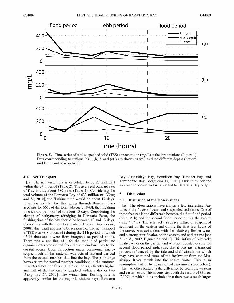
[18] Figure 5 shows the time series of TSS concentrationsat the three stations and three vertical levels. Obviously,during this observational period the TSS concentrationshows different temporal variations at each station and eachlevel. At the northeast end of the transect (station S1), thebottom TSS was high (>400 mg/L) in the beginning ofthe survey when it was flooding (Figure 6a), but it subse-quently dropped quickly and never rebounded substantially(Figure 5a). As anticipated, the bottom TSS was alwayslarger than that at the middepth; while the near surfaceconcentration was the smallest.[19] This relatively large input of TSS from the northeast

end of the transect during flood from outside of the bay isconsistent with the observed fresher water on the northeastend in the beginning of the survey [Li et al., 2009, Figure 6].This is also supported by a larger stratification on thenortheast end in the beginning of the survey [Li et al., 2009].It was speculated by Li et al. [2009] that a coastal currentfrom the outside of the bay influenced by the freshwaterfrom the Southwest Pass of the Mississippi River Delta mighthave come through either the Louisiana Coastal Current or arecirculation of an anticyclonic gyre as observed by remotesensing [Rouse and Coleman, 1976; Walker et al., 2005]and in situ observations [Murray, 1998].[20] In contrast, the southwest end of the transect started

with low TSS concentrations at all depth. This is also con-sistent with the observations of an eddy rotating counter-clockwise which had an outward flow on the southwest end.This counter current (during flood tide) was against theincoming shelf water. The TSS concentration at the south-

west end remained high (Figure 5c) for the rest of the timeperiod. The middle station S2 had a relatively low TSSconcentration most of the time except during peak ebb whenthe values increased (Figure 5b). The difference in TSSconcentration between the northeast and southwest ends isanticipated as the stratification across the transect had anout‐of‐phase oscillation as discussed in detail by Li et al.[2009].[21] The rate of integrated transport of water is more

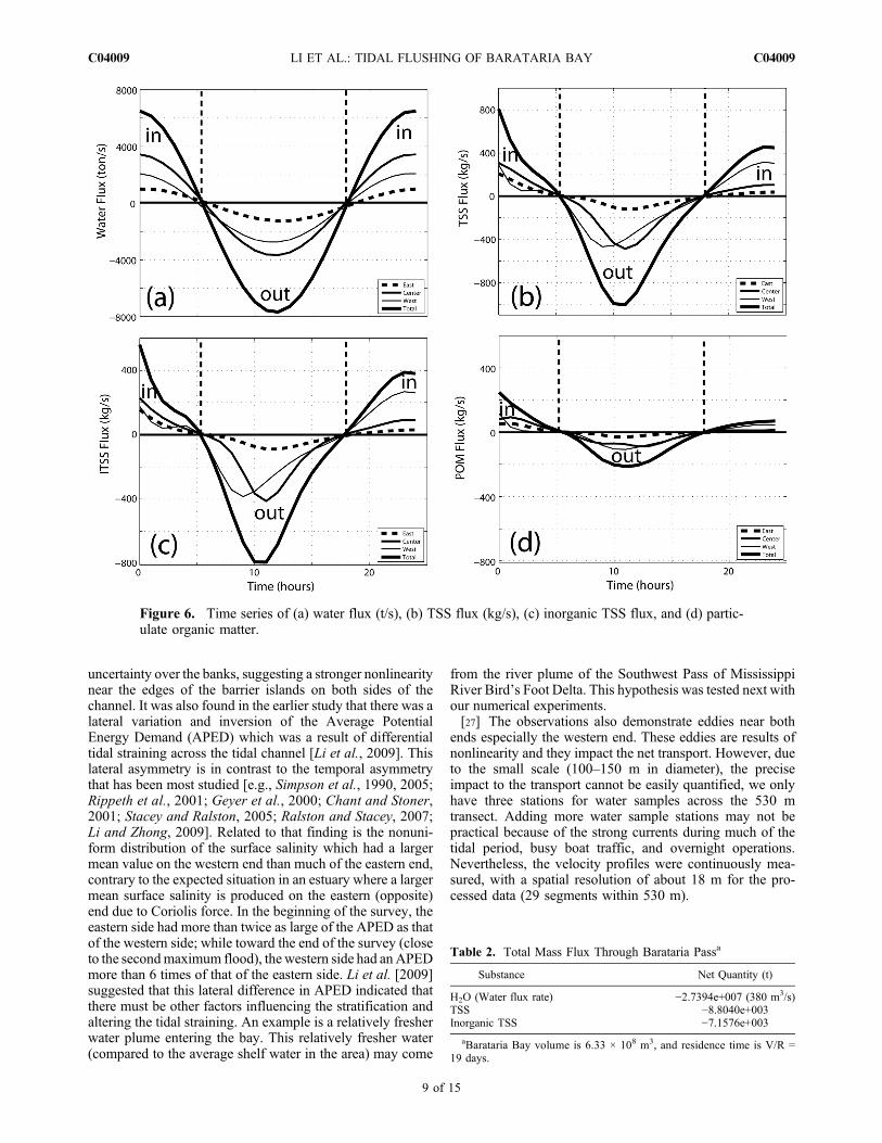
regular and has a sinusoidal pattern (Figure 6a). The totalrate of transport during peak flood is more than 6000 m3/sand close to 8000 m3/s during peak ebb; thus a net outwardflux. The northeast 1/3 of the section has the smallestmagnitude and the central 1/3 of the transect has the largestmagnitude because of the shallow water on the northeast endand deep water in the center of the channel (Figure 3). Therate of transport of water through the southwestern 1/3 of thesection is between those of the other two 1/3 sections.[22] The rate of transport of TSS is less regular and

demonstrates some nonsinusoidal variations (Figure 6b)compared to that of water (Figure 6a). The west, east, andcentral sections are not in phase for TSS transport. Duringthe peak flood the maximum inward TSS flux is 800 kg/swhile the maximum outward TSS flux is 900 kg/s.The southwest 1/3 of the section appears to have adisproportionally larger TSS flux compared to the central1/3.Within the TSS, a large fraction is inorganic (Figure 6c).The west and east/central are not in phase.[23] The TSS is composed of ∼81% of inorganic material

with the remaining composed of organic material. Conse-quently, there is a much larger flux of inorganic materialout of the bay (Figure 6c) compared to organic matter(Figure 6d) and this is consistent with the organic mattercontent of the Louisiana shelf sediments [White et al., 2009a].

Figure 4. Examples of velocity vectors showing some transient eddies at the western end of the transectduring flood stage. The velocity is from subsurface, 1.32 m below the surface. Shown for observationtimes (a) 1432–1450 and (b) 1450–1632 UT.


7 of 15

4.3. Net Transport

[24] The net water flux is calculated to be 27 million twithin the 24 h period (Table 2). The averaged outward rateof flux is thus about 380 m3/s (Table 2). Considering thetotal volume of the Barataria Bay of 633 million m3 [Fengand Li, 2010], the flushing time would be about 19 days.If we assume that the flux going through Barataria Passaccounts for 66% of the total [Marmer, 1948], then flushingtime should be modified to about 13 days. Considering thechange of bathymetry (dredging in Barataria Pass), theflushing time of the bay should be between 19 and 13 days.Comparing with the model estimate of 15 days [Inoue et al.,2008], this result appears to be reasonable. The net transportof TSS was ∼8.8 thousand t during the 24 h period, of which∼7.16 thousand t were from inorganic suspended solids.There was a net flux of 1.64 thousand t of particulateorganic matter transported from the semienclosed bay to thecoastal ocean. Upon inspection under compound micro-scope, much of this material was detrital material derivedfrom the coastal marshes that line the bay. These findingshowever are for normal weather conditions in the summer.In winter times, the flushing rate can be significantly higherand half of the bay can be emptied within a day or two[Feng and Li, 2010]. The winter time flushing rate isapparently similar for the major Louisiana bays: Barataria

Bay, Atchafalaya Bay, Vermilion Bay, Timalier Bay, andTerrebonne Bay [Feng and Li, 2010]. Our study for thesummer condition so far is limited to Barataria Bay only.

5. Discussion

5.1. Discussion of the Observations

[25] The observations have shown a few interesting fea-tures of the fluxes of water and suspended sediments. One ofthese features is the difference between the first flood period(time <5 h) and the second flood period during the survey(time >17 h). The relatively stronger influx of suspendedsediment on the eastern end during the first few hours ofthe survey was coincident with the relatively fresher waterand a strong stratification on the eastern end at that time [seeLi et al., 2009, Figures 5a and 6]. This influx of relativelyfresher water on the eastern end was not repeated during thesecond flood period, indicating that it was just a transientprocess influenced by the tide and shelf circulation whichmay have entrained some of the freshwater from the Mis-sissippi River mouth into the coastal water. This is anassumption that led to the numerical experiments (see below).[26] Another feature is the difference between the western

and eastern ends. This is consistent with the results of Li et al.[2009], in which it is concluded that there was a much larger

Figure 5. Time series of total suspended solid (TSS) concentration (mg/L) at the three stations (Figure 1).Data corresponding to stations (a) 1, (b) 2, and (c) 3 are shown as well as three different depths (bottom,middepth, and near surface).


8 of 15

uncertainty over the banks, suggesting a stronger nonlinearitynear the edges of the barrier islands on both sides of thechannel. It was also found in the earlier study that there was alateral variation and inversion of the Average PotentialEnergy Demand (APED) which was a result of differentialtidal straining across the tidal channel [Li et al., 2009]. Thislateral asymmetry is in contrast to the temporal asymmetrythat has been most studied [e.g., Simpson et al., 1990, 2005;Rippeth et al., 2001; Geyer et al., 2000; Chant and Stoner,2001; Stacey and Ralston, 2005; Ralston and Stacey, 2007;Li and Zhong, 2009]. Related to that finding is the nonuni-form distribution of the surface salinity which had a largermean value on the western end than much of the eastern end,contrary to the expected situation in an estuary where a largermean surface salinity is produced on the eastern (opposite)end due to Coriolis force. In the beginning of the survey, theeastern side had more than twice as large of the APED as thatof the western side; while toward the end of the survey (closeto the secondmaximum flood), the western side had anAPEDmore than 6 times of that of the eastern side. Li et al. [2009]suggested that this lateral difference in APED indicated thatthere must be other factors influencing the stratification andaltering the tidal straining. An example is a relatively fresherwater plume entering the bay. This relatively fresher water(compared to the average shelf water in the area) may come

from the river plume of the Southwest Pass of MississippiRiver Bird’s Foot Delta. This hypothesis was tested next withour numerical experiments.[27] The observations also demonstrate eddies near both

ends especially the western end. These eddies are results ofnonlinearity and they impact the net transport. However, dueto the small scale (100–150 m in diameter), the preciseimpact to the transport cannot be easily quantified, we onlyhave three stations for water samples across the 530 mtransect. Adding more water sample stations may not bepractical because of the strong currents during much of thetidal period, busy boat traffic, and overnight operations.Nevertheless, the velocity profiles were continuously mea-sured, with a spatial resolution of about 18 m for the pro-cessed data (29 segments within 530 m).

Figure 6. Time series of (a) water flux (t/s), (b) TSS flux (kg/s), (c) inorganic TSS flux, and (d) partic-ulate organic matter.

Table 2. Total Mass Flux Through Barataria Passa

Substance Net Quantity (t)

H2O (Water flux rate) −2.7394e+007 (380 m3/s)TSS −8.8040e+003Inorganic TSS −7.1576e+003

aBarataria Bay volume is 6.33 × 108 m3, and residence time is V/R =19 days.


9 of 15

[28] To verify our hypothesis that Mississippi River watercan enter into the Barataria Bay and to demonstrate the localsmall‐scale transient eddies, we have conducted some pro-cess oriented numerical experiments, which are discussedbelow.

5.2. Numerical Model Experiments

[29] In the process oriented numerical model experiments,we applied the Finite Volume Coastal Ocean Model(FVCOM) [Chen et al., 2003] to the entire Gulf of Mexicowith a particular focus on the northern coastal area. FVCOMhas been applied to this area in several studies for stormsurge [e.g., Rego and Li, 2010a, 2010b, 2009a, 2009b],tidally induced eddies in curved channels [Li et al., 2008],and factors influencing the seasonal hypoxia [Wang andJustic, 2009].[30] In the present work, we implemented the FVCOM to

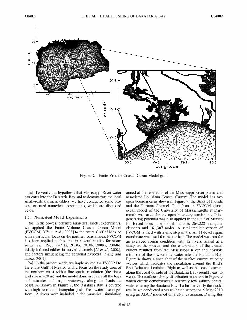
the entire Gulf of Mexico with a focus on the study area ofthe northern coast with a fine spatial resolution (the finestgrid size is ∼20 m) and the model domain covers all the baysand estuaries and major waterways along the Louisianacoast. As shown in Figure 7, the Barataria Bay is coveredwith high‐resolution triangular grids. Freshwater dischargesfrom 12 rivers were included in the numerical simulation

aimed at the resolution of the Mississippi River plume andassociated Louisiana Coastal Current. The model has twoopen boundaries as shown in Figure 7: the Strait of Floridaand the Yucatan Channel. Tide from an FVCOM globalocean model of the University of Massachusetts at Dart-mouth was used for the open boundary conditions. Tide‐generating potential was also applied in the Gulf of Mexicofor forced tides. The model includes 264,228 triangularelements and 161,307 nodes. A semi‐implicit version ofFVCOM is used with a time step of 4 s. An 11‐level sigmacoordinate was used for the vertical. The model was run foran averaged spring condition with 12 rivers, aimed at astudy on the process and the examination of the coastalcurrent resulted from the Mississippi River and possibleintrusion of the low‐salinity water into the Barataria Bay.Figure 8 shows a snap shot of the surface current velocityvectors which indicates the circulation around the Bird’sFoot Delta and Louisiana Bight as well as the coastal currentalong the coast outside of the Barataria Bay (roughly east towest). The surface salinity distribution is shown in Figure 9which clearly demonstrates a relatively low‐salinity coastalwater entering the Barataria Bay. To further verify the modelresults we conducted a vessel‐based survey on 5 May 2010using an ADCP mounted on a 26 ft catamaran. During this

Figure 7. Finite Volume Coastal Ocean Model grid.


10 of 15

survey, we used the same vessel and ADCP as we did duringthe 2008 survey at the Barataria Pass. The data presented here(Figure 10) is the near surface (∼2 m below the surface) flowvectors measured from 1903:54 to 2048:44 UTC. Thecomparison of surface current between the model andobservations are remarkably well (Figure 10). This providesconfidence to the model results of coastal current enteringinto Barataria Bay.

6. Summary

[31] In this study, a 24 h continuous survey of hydrody-namics and water sampling have allowed us to calculate theintratidal variations of fluxes and net transport of water andsuspended sediments through the Barataria Pass, the majortidal inlet of the Barataria Bay. The tidal velocity amplitudeshows a stronger magnitude on the surface in the center ofthe channel which decreases toward the banks, a conditionof frictional tide. The flow field is observed to have transienteddies at the edges of the barrier islands, which causes lowR2 values of the harmonic fit at the edges of the inlet. The

net outward flow is through the surface and both sides of theinlet, with a maximum reaching 0.5 m/s. Only a smallmagnitude (0.05 m/s) of net inward flow occurs near thebottom in deep water. This distribution of net flow field istypical in an estuary with a triangular cross section [Wong,1994]. This is also a pattern consistent with tidally inducedexchange flow in a short estuary with a triangular crosssection [Li and O’Donnell, 2005], even though the tidallyinduced flow is from an entirely different mechanism in abarotropic environment. The west side however shows amuch larger outward flow than the east side. This is coin-cident with a fresher east side, which suggests that theLouisiana Coastal Current around the Birdfoot delta derivedfrom the mixing of shelf water with the Mississippi Riverfreshwater may have entered the Bay, mostly from the eastside during the survey, which results in a smaller outwardflow on the eastern side.[32] The net flux of water is calculated to be 380 m3/s

with a total of 27 million t in weight in 24 h period whichresults in an estimate of the flushing time for the BaratariaBay to be 13–19 days. The total flux of suspended solid is

Figure 8. A typical surface current pattern from the numerical experiments.


11 of 15

estimated to be ∼9000 t, of which 80% was inorganicsuspended sediment. A process‐oriented numerical modelsimulation using a high‐resolution Finite Volume CoastalOcean Model (FVCOM) shows that relatively fresh watercan intrude into Barataria Bay through the inlets as aresult of the expansion of the Mississippi River plume andLouisiana Coastal Current, supporting the hypothesis thatriver water may come from outside of the bay, furtherconfirming our finding of an abnormal stratification varia-tion across the inlet in a earlier publication on asymmetry oftidal straining [Li et al., 2009]. The model is verified byfield observations on 5 May 2010.[33] The physical processes that affect the magnitude of

velocity, vertical mixing and stratification, and bottom tur-bulence, also affect the suspended sediment transport. Thestudy presented here is for typical summer conditions inwhich wind is weak and stratification more pronounced asthe weak vertical mixing due to lack of wind stirring coin-cides with strong surface heating. As mentioned earlier,Bataratia Bay water interacts with the Louisiana shelf water,

which is in turn influenced by the Mississippi River water.Outside of the Bay is the world second largest hypoxia zone,occurring in the summer, second only to that in the BalticSea. Southern Louisiana is also well known for its rapid rateof land loss. With 30% of the coastal marsh area, Louisianaaccounts for 90% of its loss [Dahl, 2000]. All these high-light the importance of the flushing of the bays and thesuspended sediment transport between Louisiana bays andthe Louisiana shelf. The flushing of the Louisiana bays inthe winter is largely controlled by cold fronts formed bylarge‐scale weather systems that occur at 3–7 day intervals[Roberts et al., 1989; Walker and Hammack, 2000; Fengand Li, 2010; Li et al., 2011]. This study provides themost detailed sample over a 24 h period for this system,quantifying the rate of flushing (or residence time) and thenet transport of water and sediments. The data will be usefulfor model validation for studying the flushing process of theLouisiana bays. In addition, the finding of this study aboutthe intrusion of Mississippi River water into the bay throughthe eastern side of the channel implies more complex

Figure 9. A typical surface distribution of salinity.


12 of 15

interaction between the bay and shelf waters. Obviously, thedetails of the dynamics of this interaction are yet to be fullyexplored. Our study provides more motivation for furtherstudies and more questions than answers.

[34] Acknowledgments. The research was supported by NSF (DEB‐0833225), and two NOAA grants, NA06NPS4780197 for NGoMEX fundedto LUMCON and LSU and NA06OAR4320264–06111039 to the NorthernGulf Institute by NOAA’s Office of Ocean and Atmospheric Research, theU.S. Department of Commerce, and Shell (http://www.ngi.lsu.edu/). Thework is also partially supported by the Shanghai Ocean University Programfor International Cooperation (A‐2302‐10‐0003) and the Program of Scienceand Technology Commission of Shanghai Municipality (09320503700). Wewould particularly like to thank Charlie Sibley, Chris Cleaver, DarrenDepew, Steve Jones, and Rodney Fredericks for the field work. We appreci-ate the detailed comments by two anonymous reviewers that resulted inthe improvement of the paper.

ReferencesBenke, A. C., and C. E. Cushing (2005), Rivers of North Americ, 1144 pp.,Elsevier, San Diego, Calif.

Chant, R. J., and A. W. Stoner (2001), Particle trapping in a stratifiedflood‐dominated estuary, J. Mar. Res., 59, 29–51, doi:10.1357/002224001321237353.

Chen, C., H. Liu, and R. Beardsley (2003), An unstructured grid, finite‐volume, three‐dimensional, primitive equations ocean model: Applica-tion to coastal ocean and estuaries, J. Atmos. Oceanic Technol., 20,159–186, doi:10.1175/1520-0426(2003)020<0159:AUGFVT>2.0.CO;2.

Dahl, T. E. (2000), Status and trends of wetlands in the conterminousUnited States 1986 to 1997, report, 84 pp., U. S. Dep. of the Inter., Fishand Wildl., Washington, D. C.

Feng, Z., and C. Li (2010), Cold‐front‐induced flushing of the Louisianabays, J. Mar. Syst., 82, 252–264, doi:10.1016/j.jmarsys.2010.05.015.

Geyer, W. R., J. H. Trowbridge, and M. M. Bowen (2000), The dynamicsof a partially mixed estuary, J. Phys. Oceanogr., 30, 2035–2048.

Goñi, M. A., G. Voulgaris, and Y. H. Kim (2009), Composition and fluxesof particulate organic matter in a temperate estuary (Winyah Bay, SouthCarolina, USA) under contrasting physical forcings, Estuarine CoastalShelf Sci., 85, 273–291, doi:10.1016/j.ecss.2009.08.013.

Inoue, M., and W. J. Wiseman Jr. (2000), Transport, mixing and stirringprocesses in a Louisiana estuary, Estuarine Coastal Shelf Sci., 50,449–466, doi:10.1006/ecss.2000.0587.

Inoue,M., D. Park, D. Justic, andW. J.Wiseman Jr. (2008), A high‐resolutionintegrated hydrology‐hydrodynamic model of the Barataria Basin system,Environ.Model. Softw., 23, 1122–1132, doi:10.1016/j.envsoft.2008.02.011.

Joyce, T. M. (1989), On in situ calibration of shipboard ADCPs, J. Atmos.Oceanic Technol., 6, 169–172, doi:10.1175/1520-0426(1989)006<0169:OISOSA>2.0.CO;2.

Justic, D., V. J. Bierman Jr., D. Scavia, and R. D. Hetland (2007), Forecast-ing Gulf’s hypoxia: The next 50 years?, Estuaries Coasts, 30, 791–801.

Figure 10. Comparison of model results (thin arrows) and observed surface currents (thick arrows) on5 May 2010.


13 of 15

Kantha, L. (2005), Barotropic tides in the Gulf of Mexico, in Circulation inthe Gulf of Mexico: Observations and Models, Geophys. Monogr. Ser.,vol. 161, edited by W. Sturges and A. Lugo‐Fernandez, pp. 159–163,AGU, Washington, D. C.

Kayhanian, M., E. Rasa, A. Vichare, and J. E. Leatherbarrow (2008),Utility of suspended solid measurements for storm‐water runoff treatment,J. Environ. Eng., 134, 712–721, doi:10.1061/(ASCE)0733-9372(2008)134:9(712).

Kjerfve, B. (1978), Bathymetry as an indicator of net circulation inwell‐mixedestuaries, Limnol. Oceanogr., 23, 816–821, doi:10.4319/lo.1978.23.4.0816.

Kjerfve, B., L. H. Stevenson, J. A. Proehl, and T. H. Chrzanowski (1981),Estimation of material fluxes in an estuarine cross section: A critical anal-ysis of spatial measurement density and errors, Limnol. Oceanogr., 26,325–335, doi:10.4319/lo.1981.26.2.0325.

Li, C. (2001), 3Danalyticmodel for testing numerical tidalmodels, J.Hydraul.Eng., 127, 709–717, doi:10.1061/(ASCE)0733-9429(2001)127:9(709).

Li, C. (2002), Axial convergence fronts in a barotropic tidal inlet—Sand shoalinlet, VA, Cont. Shelf Res., 22, 2633–2653, doi:10.1016/S0278-4343(02)00118-8.

Li, C., and J. O’Donnell (2005), The effect of channel length on the resid-ual circulation in tidally dominated channels, J. Phys. Oceanogr., 35,1826–1840, doi:10.1175/JPO2804.1.

Li, C., and A. Valle‐Levinson (1999), A two‐dimensional analytic tidal modelfor a narrow estuary of arbitrary lateral depth variation: The intratidal motion,J. Geophys. Res., 104, 23,525–23,543, doi:10.1029/1999JC900172.

Li, C., and E. Weeks (2009), Measurements of a small scale eddy at a tidalinlet using an unmanned automated boat, J. Mar. Syst., 75, 150–162,doi:10.1016/j.jmarsys.2008.08.007.

Li, C., A. Valle‐Levinson, K.‐C.Wong, and K. M.M. Lwiza (1998), Separat-ing baroclinic flow from tidally induced flow in estuaries, J. Geophys. Res.,103, 10,405–10,417, doi:10.1029/98JC00582.

Li, C., A. Valle‐Levinson, L. P. Atkinson, and T. C. Royer (2000), Infer-ence of tidal elevation in shallow water using a vessel‐towed acousticDoppler current profiler, J. Geophys. Res., 105, 26,225–26,236,doi:10.1029/1999JC000191.

Li, C., J. O. Blanton, and C. Chen (2004), Mapping of tide and tidal flowsusing vessel towed ADCP, J. Geophys. Res., 109, C04002, doi:10.1029/2003JC001992.

Li, C., C. Chen, D. Guadagnoli, and I. Y. Georgiou (2008), Geometry‐inducedresidual eddies in estuaries with curved channels: Observations and model-ing studies, J. Geophys. Res., 113, C01005, doi:10.1029/2006JC004031.

Li, C., E. Swenson, E. Weeks, and J. White (2009), Asymmetric tidal strain-ing across an inlet: Lateral inversion and variability over a tidal cycle,Estu-arine Coastal Shelf Sci., 85, 651–660, doi:10.1016/j.ecss.2009.09.015.

Li, C., H. Roberts, G. Stone, E.Weeks, andY. Luo (2011),Wind surge and salt-water intrusion in Atchafalaya Bay under onshore winds prior to cold frontpassage, Hydrobiologia, 658, 27–39, doi:10.1007/s10750-010-0467-5.

Li, M., and L. Zhong (2009), Flood‐ebb and spring‐neap variations of mix-ing, stratification and circulation in Chesapeake Bay, Cont. Shelf Res.,29, 4–14, doi:10.1016/j.csr.2007.06.012.

Linden, P. F., and J. E. Simpson (1988), Modulated mixing and frontogen-esis in shallow seas and estuaries, Cont. Shelf Res., 8, 1107–1127,doi:10.1016/0278-4343(88)90015-5.

Makarewicz, J. C., T. W. Lewis, I. Bosch, M. R. Noll, N. Herendeen, R. D.Simon, J. Zollweg, and A. Vodacek (2009), The impact of agriculturalbest management practices on downstream systems: Soil loss and nutri-ent chemistry and flux to Conesus Lake, New York, USA, J. Great LakesRes., 35, 23–36, doi:10.1016/j.jglr.2008.10.006.

Marmer, H. A. (1948), The currents in Barataria Bay, report, 30 pp., Tex.A&M Res. Found., College Station, Tex.

Murray, S. P. (1998), An observational study of the Mississippi‐Atchafalayacoastal plume: Final report, OCS Study MMS Rep. 98‐0040, 513 pp., Gulfof Mex. Outer Cont. Shelf Reg., Miner. Manage. Serv., U. S. Dep. of theInter., New Orleans, La.

Nahlik, A. M., and W. J. Mitsch (2008), The effect of river pulsing on sed-imentation and nutrients in created Riparian wetlands, J. Environ. Qual.,37, 1634–1643, doi:10.2134/jeq2007.0116.

Nunes, R. A., and G. W. Lennon (1987), Episodic stratification and gravitycurrents in a marine environment of modulated turbulence, J. Geophys.Res., 92, 5465–5480, doi:10.1029/JC092iC05p05465.

Nunes Vaz, R. A., G. W. Lennon, and J. R. de Silva Samarasinghe (1989),The negative role of turbulence in estuarine mass transport, EstuarineCoastal Shelf Sci., 28, 361–377, doi:10.1016/0272-7714(89)90085-1.

Park, D. (2002), Hydrodynamics and freshwater diversion within BaratariaBasin, Ph.D. dissertation, 112 pp., La. State Univ., Baton Rouge.

Rabalais, N. N., and R. E. Turner (Eds.) (2001), Coastal Hypoxia: Conse-quences for Living Resources and Ecosystems, Coastal Estuarine Stud.Ser., vol. 58, AGU, Washington, D. C.

Rabalais, N. N., R. E. Turner, B. K. Sen Gupta, D. F. Boesch, P. Chapman,and M. C. Murrell (2007a), Hypoxia in the northern Gulf of Mexico:Does the science support the plan to reduce, mitigate and control hypoxia?,Estuaries Coasts, 30, 753–772.

Rabalais, N. N., R. E. Turner, B. K. Sen Gupta, E. Platon, and M. L. Parsons(2007b), Sediments tell the history of eutrophication and hypoxia in thenorthern Gulf of Mexico, Ecol. Appl., 17, suppl., S129–S143,doi:10.1890/06-0644.1.

Ralston, D. K., and M. T. Stacey (2007), Tidal and meteorological forcingof sediment transport in tributary mudflat channels, Cont. Shelf Res., 27,1510–1527, doi:10.1016/j.csr.2007.01.010.

RD Instruments (1996), Acoustic Doppler Current Profiler Principles ofOperation—A Practical Primer, 57 pp., Poway, Calif.

Rego, J., and C. Li (2009a), On the receding of storm surge along Louisiana’slow‐lying coast, J. Coastal Res., 56, 1045–1049.

Rego, J., and C. Li (2009b), Numerical experiments and an overlookedparameter in storm surge forecasting: The forward speed of a hurricane,Geophys. Res. Lett., 36, L07609, doi:10.1029/2008GL036953.

Rego, J., and C. Li (2010a), Nonlinear terms in storm surge predictions:Effect of tide and shelf geometry with case study from Hurricane Rita,J. Geophys. Res., 115, C06020, doi:10.1029/2009JC005285.

Rego, J., and C. Li (2010b), Storm surge propagation in Galveston Bay duringHurricane Ike, J. Mar. Syst., 82, 265–279, doi:10.1016/j.jmarsys.2010.06.001.

Rippeth, T. P., N. R. Fisher, and J. H. Simpson, (2001), The cycle of tur-bulent dissipation in the presence of tidal straining, J. Phys. Oceanogr., 31,2458–2471, doi:10.1175/1520-0485(2001)031<2458:TCOTDI>2.0.CO;2.

Roberts, H. H., R. D. Adams, and R. H. W. Cunningham (1980), Evolutionof sand‐dominant subaerial phase, Atchafalaya Delta, Louisiana,Am. Assoc.Pet. Geol. Bull., 64, 264–279.

Roberts, H. H., O. K. Huh, S. A. Hsu, L. J. Rouse Jr., and D. A. Rickman(1989), Winter storm impacts on the Chenier Plain Coast of southwesternLouisiana, Trans. Gulf Coast Assoc. Geol. Soc., 39, 515–522.

Roberts, H. H., N. Walker, R. Cunningham, G. P. Kemp, and S. Majersky(1997), Evolution of sedimentary architecture and surface morphology:Atchafalaya and Wax Lake Deltas, Louisiana (1973–1994), Trans. GulfCoast Assoc. Geol. Soc., 47, 477–484.

Rouse, L. J., and J. M. Coleman (1976), Circulation observations in theLouisiana Bight using LANDSAT Imagery, Remote Sens. Environ., 5,55–66, doi:10.1016/0034-4257(76)90035-3.

Simpson, J. H., J. Brown, J. Matthews, and G. Allen (1990), Tidal strain-ing, density currents, and stirring in the control of estuarine stratification,Estuaries, 13, 125–132, doi:10.2307/1351581.

Simpson, J. H., E. Williams, L. H. Brasseur, and J. M. Brubaker (2005),The impact of tidal straining on the cycle of turbulence in a partially strat-ified estuary, Cont. Shelf Res., 25, 51–64, doi:10.1016/j.csr.2004.08.003.

Snedden, G. A. (2006), River, tidal and wind interactions in a deltaic estu-arine system, Ph.D. dissertation, 116 pp., La. State Univ., Baton Rouge.

Stacey, M. T., and D. K. Ralston (2005), The scaling and structure of theestuarine bottom boundary layer, J. Phys. Oceanogr., 35, 55–71,doi:10.1175/JPO-2672.1.

Swenson, E. M., and C. M. Swarzenski (1995), Water levels and salinity inthe Barataria‐Terrebonne Estuarine system, in Status and Trends of Hydro-logic Modification, Reduction in Sediment Availability, and Habitat Loss/Modification in the Barataria and Terrebonne Estuarine System,Barataria‐Terrebonne Natl. Estuarine Program Publ. Ser., vol. 20, editedby D. J. Reed, pp. 130–215, Barataria‐Terrebonne Natl. Estuary Program,Thibodaux, La.

Uthicke, S., and K. Nobes (2008), Benthic foraminifera as ecological indi-cators for water quality on the Great Barrier Reef, Estuarine CoastalShelf Sci., 78, 763–773, doi:10.1016/j.ecss.2008.02.014.

Walker, N. D., and A. B. Hammack (2000), Impacts of winter storms oncirculation and sediment transport: Atchafalaya‐Vermillion Bay region,Louisiana. U.S.A., J. Coastal Res., 16, 996–1010.

Walker, N., W. J. Wiseman Jr., L. J. Rouse Jr., and A. Babin (2005), Effectsof river discharge, wind stress, and slope eddies on circulation and the sat-ellite‐observed structure of the Mississippi River plume, J. Coastal Res.,21, 1228–1244, doi:10.2112/04-0347.1.

Wang, L., and D. Justic (2009), A modeling study of the physical processesaffecting the development of seasonal hypoxia over the inner Louisiana‐Texas shelf: Circulation and stratification, Cont. Shelf Res., 29, 1464–1476,doi:10.1016/j.csr.2009.03.014.

White, J. R., R. D. DeLaune, C. Y. Li, and S. Bentley (2009a), Distributionof methyl and total mercury in Louisiana and Georgia shelf sediments,Anal. Lett., 42, 1219–1231, doi:10.1080/00032710902901947.

White, J. R., R.W. Fulweiler, C. Y. Li, S. Bargu, N. D.Walker, R. R. Twilley,and S. E. Green (2009b), Mississippi River flood of 2008: Observations ofa large freshwater diversion on physical, chemical and biological charac-teristics of a shallow estuarine lake,Environ. Sci. Technol., 43, 5599–5604.


14 of 15

Wong, K.‐C. (1994), On the nature of transverse variability in a coastal plainestuary, J. Geophys. Res., 99, 14,209–14,222, doi:10.1029/94JC00861.

S. Bargu, K. Galvan, C. Li, E. Weeks, and J. R. White, Department ofOceanography and Coastal Sciences, Louisiana State University, BatonRouge, LA 70803, USA. ([email protected])

C. Chen and H. Lin, Department of Fisheries Oceanography, IntercampusGraduate School for Marine Science and Technology, University ofMassachusetts, New Bedford, MA 02744, USA.


15 of 15

Documents

Summertime tidal flushing of Barataria Bay: Transports …fvcom.smast.umassd.edu/wp-content/uploads/2013/12/Li_etal_2011... · Summertime tidal flushing of Barataria Bay: Transports