Embed Size (px)
Citation preview

Dynamic MacroeconomicsSummer Term 2011
Christian Bayer
Universität Bonn
May 15, 2011
C. Bayer Dynamic Macro

Overview of the Course: My Part
1. Introduction, Basic Theory
2. Stochastic Fluctuations
3. Numerical Tools
4. Estimation
5. Equilibrium
6. Stationary heterogenous agent economies
7. Heterogeneous agent economies with aggregate fluctuations
C. Bayer Dynamic Macro

Literature
Primary reading:
I Heer, B. and A. Maussner (2009), "Dynamic General EquilibriumModelling", 2nd edition, Springer, Berlin.I cover roughly: Ch. 1, 4, 7, 8
Secondary reading:
I Adda, J. and R. Cooper (2004): "Dynamic Economics", MIT Press,Cambridge.
I Ljungqvist, L. und T. Sargent (2004): "Recursive MacroeconomicTheory", MIT press, Cambridge.
I Stockey, N.L. and Lucas, R.E. with E.C. Prescott (1989): "RecursiveMethods in Economic Dynamics", Chapters 4 and 9, HavardUniversity Press, Cambridge..
C. Bayer Dynamic Macro

Motivation:The standard incomplete markets model
Hugget (1993), Aiyagari (1994) and Krussel and Smith (1998)
C. Bayer Dynamic Macro

What we want to model...
I Consider an economy in which households supply labor, consumeand accumulate capital.
I They each face idiosyncratic risk as their endowment with effi ciencyunits of labor changes over time (they may be employed orunemployed for example).
I Other than in a standard (i.e. complete markets) macro model, wewant to assume that households cannot trade away theiridiosyncratic risk on complete asset markets (there is no perfectunemployment insurance).
I We want to assume that the only asset households can trade is aclaim on the aggregate stock of capital.
I We want to understand the quantitative implications.
C. Bayer Dynamic Macro

What do we need to model...
I How households make their consumption-savings decisions givenprices (forward looking behavior)?
I Heterogeneity of households in wealthI The effect of aggregate fluctuations on this heterogeneity and itsrepercussions on prices.
C. Bayer Dynamic Macro

Households
Putting this a little more formally:
I Continuum of households that obtain income from supplying labornt and assets at at prices wt and rt respectively.
I Households enjoy utility from consumption ct , are expected utilitymaximizers and are infinitely lived.
I They discount future utility by the discount factor β.
I [Labour supply nt ∈ [nmin, nmax] is an exogenous stochastic process.]
C. Bayer Dynamic Macro

Budget and borrowing constraints
I We want to assume (following Aiyagari, 1994) that there are nocontingent claims households can trade.
I Households can only self-insure using the asset a.I Asset holdings must satisfy that the household is able to serviceeventual debt in any case
a′ ≥ bI b is an exogenous debt limit (necessary to avoid Ponzi schemes ifr < 0). We will typically set b = 0.
C. Bayer Dynamic Macro

Household Planning ProblemSetup
I The planning problem of each households can be summarized in theBellman equation
max<at>t=1...∞at∈R+
E0∞
∑t=0
βtu (wtnt + at (1+ rt )− at+1)
I where the sequence < at > is contingent on the history ofrealizations for (wt , rt , nt ,Zt )
I Zt is an aggregate state of the economy that determines theprobability distributions for nt , i.e. it determines aggregateemployment.
C. Bayer Dynamic Macro

Household Planning ProblemIssues in Solving
I The planning problem
max<at>t=1...∞at∈R+
E0∞
∑t=0
βtu (wtnt + at (1+ rt )− at+1)
yields in general first order conditions, with occasionally bindingconstraints.
−βtu′ (ct ) + βt+1 (1+ rt ) u′ (ct+1) = λt
where λt is the Lagrangian multiplier on the non-negativityconstraint for at .
I This cannot be solved using local approximations!I Another diffi culty arises in form of the prices (wt , rt ), which mayfluctuate with aggregate employment and households need to formexpectations about these price movements.
C. Bayer Dynamic Macro

Overview of Course ProgrammeTheory of Dynamic Programming
Numerical Analysis
Part 1Introduction,
Dynamic Programming: Basic Theoryand First Numerical Tools
C. Bayer Dynamic Macro

Overview of Course ProgrammeTheory of Dynamic Programming
Numerical Analysis
TheoryNumerics
The Theory of Dynamic Programming
1. Back to Consumption Theory 101: Indirect Utility and ValueFunctions
2. Basic dynamic programming in a finite horizon environment
3. Stationary Problems and Infinite Horizon Dynamic Programming
4. Stochastic Dynamic Programming
5. Analytical Solutions and Numerical Analysis
C. Bayer Dynamic Macro

Overview of Course ProgrammeTheory of Dynamic Programming
Numerical Analysis
TheoryNumerics
Numerical Analysis of Dynamic Programming Problems
1. Continuous vs. discrete decision problems
2. Discrete Approximations to a Continuous State Space
3. Value Function Iteration
4. Transition Probability Matrices and Markov Chain
5. Autoregressions and Tauchen’s Algorithm
C. Bayer Dynamic Macro

Overview of Course ProgrammeTheory of Dynamic Programming
Numerical Analysis
Indirect utilityFinite time horizonInifinite time horizonRamsey EconomyStochastic stationary dynamic programming
Indirect Utility
Recall from consumer theory the concept of indirect utility:
V (p, I ) = maxc≥0
u (c) , s.t. pc ≤ I .
Reflects the highest utility level, a household can achieve by consumptionchoice, given his income I and the price vector p.
I We can think of (p, I ) as indexing the state of the economy.I Therefore we will call (p, I ) the state vector.
C. Bayer Dynamic Macro

Overview of Course ProgrammeTheory of Dynamic Programming
Numerical Analysis
Indirect utilityFinite time horizonInifinite time horizonRamsey EconomyStochastic stationary dynamic programming
Profit functions
I Analogously, we have the concept of a (short-run) profit function inproduction theory:
Π (p,w ,K ) = maxLpF (K , L)− wL− rK .
I Again, we can think of (p,w ,K ) as indexing the state of theeconomy for the firm.
I While the concept of indirect utility / reduced form profit functionsmainly helps in simplifying some analysis in static consumer theory(Slutsky-decomposition for example), it will turn out to be a verypowerful tool in a dynamic analysis.
C. Bayer Dynamic Macro
Overview of Course ProgrammeTheory of Dynamic Programming
Numerical Analysis
Indirect utilityFinite time horizonInifinite time horizonRamsey EconomyStochastic stationary dynamic programming
General formulation, finite time horizon
Now consider a dynamic problem of a generic form:
maxT
∑t=0
βtu (xt , xt+1) , s.t. xt+1 ∈ Γt (xt ) , x0 given.
where u (xt , xt+1) is a payoff function that depends on the current statext as well as on the future state xt+1 chosen by the decision maker.
C. Bayer Dynamic Macro

Overview of Course ProgrammeTheory of Dynamic Programming
Numerical Analysis
Indirect utilityFinite time horizonInifinite time horizonRamsey EconomyStochastic stationary dynamic programming
General formulation, finite time horizon
Denoting the indirect utility obtained as V (xt , t) , we can restate theProblem as a so called Bellman equation
V (xt , t) = u (xt , xt+1) + βV (xt+1, t + 1) , s.t. xt+1 ∈ Γt (xt ) .
where V exists if Γ is compact valued (Theorem of the Maximum).The time-index t reflects the fact that it matters how many remainingperiods there are.With finite horizon the optimization problem is necessarilynon-stationary, i.e. changes with time t.
C. Bayer Dynamic Macro

Overview of Course ProgrammeTheory of Dynamic Programming
Numerical Analysis
Indirect utilityFinite time horizonInifinite time horizonRamsey EconomyStochastic stationary dynamic programming
A cake eating example
To fix ideas consider the usage of a depletable resource (cake-eating)
maxT
∑t=0
βtu (ct ) , s.t. Wt+1 = Wt − ct , ct ≥ 0, W0 given.
To put this in the general form, expressing the problem only in terms ofstate variables Wt we replace ct = Wt −Wt+1
maxT
∑t=0
βtu (Wt −Wt+1) , s.t. Wt+1 ≤ Wt .
C. Bayer Dynamic Macro

Overview of Course ProgrammeTheory of Dynamic Programming
Numerical Analysis
Indirect utilityFinite time horizonInifinite time horizonRamsey EconomyStochastic stationary dynamic programming
A cake eating example
As formulation in terms of the Bellman equation, we obtain
V (Wt , t) = max u (Wt −Wt+1) + βV (Wt+1, t + 1) , s.t. Wt+1 ≤ Wt .
C. Bayer Dynamic Macro

Overview of Course ProgrammeTheory of Dynamic Programming
Numerical Analysis
Indirect utilityFinite time horizonInifinite time horizonRamsey EconomyStochastic stationary dynamic programming
Bellman equations and infinite time horizon
While the dynamic programming (Bellman equation) approach generatessomewhat more information about the optimization problem in a finitehorizon setup than a direct attack on the problem, it is at the same timemore burdensome, since we need to determine V for each t.It becomes a powerful approach really only when we look at infinite timehorizon problems.These can be stationary, i.e. does not change in t, as the remainingtime until the end of the decision problem remains always ∞.
C. Bayer Dynamic Macro

Overview of Course ProgrammeTheory of Dynamic Programming
Numerical Analysis
Indirect utilityFinite time horizonInifinite time horizonRamsey EconomyStochastic stationary dynamic programming
Stationary dynamic programming
If the problem is stationary (and a solution does exist), we can state theplanning problem as
V (x) = max u (x , y) + βV (y) s.t. y ∈ Γ (x) .
I Note however that not all infinite horizon problems are stationary.Sometimes a problem can be reformulated in stationary terms (Youknow that from econometrics).
I Also note that a solution may not exist.I The unknown of the Bellman equation is the function V (x)
C. Bayer Dynamic Macro

Overview of Course ProgrammeTheory of Dynamic Programming
Numerical Analysis
Indirect utilityFinite time horizonInifinite time horizonRamsey EconomyStochastic stationary dynamic programming
An ExampleThe neo-classical growth model
A social planner wants to maximize the stream of utility fromconsumption in an economy, where
U = U (Ct )
Yt = Ct + It ; Yt = K αt
Kt+1 = (1− δ)Kt + It
V (K0) = max<Kt>t=1...∞
∞
∑t=0
βtU [C (Kt ,Kt+1)]
s.t. C = K αt + (1− δ)Kt −Kt+1
Kt+1 ≥ 0
Kt+1 ≤ K αt + (1− δ)Kt
C. Bayer Dynamic Macro

Overview of Course ProgrammeTheory of Dynamic Programming
Numerical Analysis
Indirect utilityFinite time horizonInifinite time horizonRamsey EconomyStochastic stationary dynamic programming
An ExampleThe neo-classical growth model
We can rewrite this as
V (K ) = max<Kt>t=1...∞
∞
∑t=0
βtU [C (Kt ,Kt+1)] with Kt = K
= maxKt+1
{u (K ,Kt+1) + max
<Kt+1>t=1...∞β
∞
∑t=0
βtu [C (Kt+1,Kt+2)]
}= max
K ′∈Γ(K )
{u(K ,K ′
)+ βV
(K ′)}
Γ (K ) : = {k ∈ R+| k ≤ K α + (1− δ)K}u (K ,Kt+1) : = U [C (Kt ,Kt+1)]
C. Bayer Dynamic Macro

Overview of Course ProgrammeTheory of Dynamic Programming
Numerical Analysis
Indirect utilityFinite time horizonInifinite time horizonRamsey EconomyStochastic stationary dynamic programming
When does a solution exist?
We can formulate the Bellman equation as a mapping
U (x) = T (V (x))
T [V (x)] = maxyu (x , y) + βV (y) s.t. y ∈ Γ (x) (1)
that maps function V to a new function U.
C. Bayer Dynamic Macro

Overview of Course ProgrammeTheory of Dynamic Programming
Numerical Analysis
Indirect utilityFinite time horizonInifinite time horizonRamsey EconomyStochastic stationary dynamic programming
Some prerequisits
DefinitionA sequence (xn) is said to be a Cauchy sequence on the metric space(C , d) if for all ε > 0 there exists a n (ε) , such that for allm, n ≥ n (ε) : d (xm , xn) < ε.
LemmaIn a complete metric space, all Cauchy sequences converge, i.e. for anyCauchy sequence (xn) , there is an x ∈ C , such that d (xn , x)→ 0 asn→ ∞. (without proof)
C. Bayer Dynamic Macro

Overview of Course ProgrammeTheory of Dynamic Programming
Numerical Analysis
Indirect utilityFinite time horizonInifinite time horizonRamsey EconomyStochastic stationary dynamic programming
Some prerequisits
DefinitionThe mapping T is a contraction on the complete metric space {C , d} iffor any x , y ∈ C ⇒ Tx ,Ty ∈ C and for some ρ < 1 :d (Tx ,Ty) ≤ ρd (x , y) .
LemmaIf T is a contraction then T nx is a Cauchy sequence (to be proof asExcercise 1).
RemarkNote that the set of continuous bounded functions is a complete metricspace, with the sup-norm as metric.
C. Bayer Dynamic Macro

Overview of Course ProgrammeTheory of Dynamic Programming
Numerical Analysis
Indirect utilityFinite time horizonInifinite time horizonRamsey EconomyStochastic stationary dynamic programming
Exercise 1
Show that if T is a contraction then T nx is a Cauchy sequence !
C. Bayer Dynamic Macro

Overview of Course ProgrammeTheory of Dynamic Programming
Numerical Analysis
Indirect utilityFinite time horizonInifinite time horizonRamsey EconomyStochastic stationary dynamic programming
Existence of a Solution to the Bellman equationThe contraction mapping theorem
TheoremIf the Bellman equation (1) defines T to be a contraction mapping onthe set of continuous bounded functions, then a solution to (1) exists.
C. Bayer Dynamic Macro

Overview of Course ProgrammeTheory of Dynamic Programming
Numerical Analysis
Indirect utilityFinite time horizonInifinite time horizonRamsey EconomyStochastic stationary dynamic programming
Existence
Proof.1.) note that if (1) has a solution, then it is a fixed point of T and viceversa.2.) if the contraction mapping T has a fixed point, then it is unique: Let
Tx = x ,Ty = y ⇒d (x , y) = d (Tx ,Ty) ≤ ρd (x , y)
⇒ d (x , y) = 0
⇒ x = y
C. Bayer Dynamic Macro

Overview of Course ProgrammeTheory of Dynamic Programming
Numerical Analysis
Indirect utilityFinite time horizonInifinite time horizonRamsey EconomyStochastic stationary dynamic programming
Existence
Proof.3.) T is continuous, i.e. yn → y ⇒ Tyn → Ty as
d (Tyn ,Ty) ≤ ρd (yn , y)n→∞→ 0
⇒ Tyn → Ty
4.) the limit limn→∞ T nx =: x∗ exists because T nx is Cauchy (seeExercise 1).
5.) this implies
Tx∗ = T(limn→∞
T nx)
= limn→∞
TT nx = limn→∞
T n+1x = x∗,
so that x∗ is the fixed point of T , which concludes the proof.
C. Bayer Dynamic Macro

Overview of Course ProgrammeTheory of Dynamic Programming
Numerical Analysis
Indirect utilityFinite time horizonInifinite time horizonRamsey EconomyStochastic stationary dynamic programming
An algorithm to solve the Bellman equation
The proof to show existence of a solution to the Bellman equation isconstructive. It tells us how to find a solution to the Bellman equation:
1. Show that T is a contraction.
2. Start with some initial guess V0 and then construct a sequenceVn = TVn−1.
3. After a suffi ciently large number of iterations Vn will becomearbitrarily close to the solution V .
4. This algorithm is called "Value-Function-Iteration" (VFI).
C. Bayer Dynamic Macro

Overview of Course ProgrammeTheory of Dynamic Programming
Numerical Analysis
Indirect utilityFinite time horizonInifinite time horizonRamsey EconomyStochastic stationary dynamic programming
Blackwell’s condition
TheoremIf T fulfills the following conditions, then T is a contraction mapping onthe set of bounded and continuous functions:
1. T preserves boundedness.
2. T preserves continuity.
3. T is monotonic: w ≥ v ⇒ Tw ≥ Tv4. T satisfies discounting, i.e. there is some 0 ≤ β < 1, such that forany real valued constant c and any function v we haveT (v + c) ≤ Tv + βc .
C. Bayer Dynamic Macro

Overview of Course ProgrammeTheory of Dynamic Programming
Numerical Analysis
Indirect utilityFinite time horizonInifinite time horizonRamsey EconomyStochastic stationary dynamic programming
A solution exists in the generic case
Theorem (Existence of the value function)Assume u (x , x ′) is real-valued, continuous, and bounded, 0 < β < 1,and that the constraint set Γ (s) is a non-empty, compact-valued, andcontinuous correspondence. Then there exists a unique continuous valuefunction V (s) that solves the Bellman equation (1) .
C. Bayer Dynamic Macro

Overview of Course ProgrammeTheory of Dynamic Programming
Numerical Analysis
Indirect utilityFinite time horizonInifinite time horizonRamsey EconomyStochastic stationary dynamic programming
Policy function
Theorem (Existence of the policy function)Assume u (x , x ′) is real-valued, continuous, strictly concave andbounded, 0 < β < 1, and that the set of potential states is a convexsubset of Rk and the constraint set Γ (s) is a non-empty,compact-valued, continuous, and convex correspondence. Then theunique value function V (s) is continuous and strictly concave. Moreoverthe optimal policy
φ (x) := arg maxy∈Γ(x )
u (x , y) + βV (x)
is a continuous (single-valued) function.
C. Bayer Dynamic Macro

Overview of Course ProgrammeTheory of Dynamic Programming
Numerical Analysis
Indirect utilityFinite time horizonInifinite time horizonRamsey EconomyStochastic stationary dynamic programming
A simple optimal capital accumulation model
I To put things into practice, we consider the Ramsey-Cass-Koopmansgrowth model in a simplified version:
I Consider a household having a utility function
u (ct , nt ) = ln (ct )
I The consumption good is produced from a depreciating capital good:
yt = zkαt , 0 < α < 1,
kt+1 = kt (1− δ) + it , 0 ≤ δ ≤ 1,yt = ct + it .
C. Bayer Dynamic Macro

Overview of Course ProgrammeTheory of Dynamic Programming
Numerical Analysis
Indirect utilityFinite time horizonInifinite time horizonRamsey EconomyStochastic stationary dynamic programming
A simple optimal capital accumulation model
1. How can we put this into the terms of dynamic programming?
2. Consumption is the policy variable.3. Capital is the state variable.4.
V (kt ) = maxct≤yt−ityt=Ak α
tkt+1=kt (1−δ)+it
ln (ct ) + βV (kt+1) .
5. This problem fulfills all assumptions of our 2 central theorems.
C. Bayer Dynamic Macro

Overview of Course ProgrammeTheory of Dynamic Programming
Numerical Analysis
Indirect utilityFinite time horizonInifinite time horizonRamsey EconomyStochastic stationary dynamic programming
Well this looks like a simple model, ....
I but ...I You’ll need a computer to solve it.I Unless you fix δ to 1,I which is what we will do for didactical reasons:
1. We learn to understand the problem2. We can compare approximate numerical solutions to the "true"analytical solution
C. Bayer Dynamic Macro

Overview of Course ProgrammeTheory of Dynamic Programming
Numerical Analysis
Indirect utilityFinite time horizonInifinite time horizonRamsey EconomyStochastic stationary dynamic programming
Full depreciation
I Now the Problem takes the form
V (k) = maxk ′≤Ak α+k (1−δ)
ln(zkα − k ′
)+ βV
(k ′).
I Guess that V (k) = A+ B ln (k) .I This yields the FOC for the optimal policy
− 1zkα − k ′ + βV ′
(k ′)= 0
C. Bayer Dynamic Macro

Overview of Course ProgrammeTheory of Dynamic Programming
Numerical Analysis
Indirect utilityFinite time horizonInifinite time horizonRamsey EconomyStochastic stationary dynamic programming
Full depreciation
I Now the Problem takes the form
V (k) = maxk ′≤Ak α+k (1−δ)
ln(zkα − k ′
)+ βV
(k ′).
I Guess that V (k) = A+ B ln (k) .I Plugging in the guess for V :(
zkα − k ′)−1
= βBk ′−1
C. Bayer Dynamic Macro

Overview of Course ProgrammeTheory of Dynamic Programming
Numerical Analysis
Indirect utilityFinite time horizonInifinite time horizonRamsey EconomyStochastic stationary dynamic programming
Full depreciation
I Now the Problem takes the form
V (k) = maxk ′≤Ak α+k (1−δ)
ln(zkα − k ′
)+ βV
(k ′).
I Guess that V (k) = A+ B ln (k) .I Plugging in the guess for V :
βB(zkα − k ′
)= k ′
C. Bayer Dynamic Macro
Overview of Course ProgrammeTheory of Dynamic Programming
Numerical Analysis
Indirect utilityFinite time horizonInifinite time horizonRamsey EconomyStochastic stationary dynamic programming
Full depreciation
1. Now the Problem takes the form
V (k) = maxk ′≤Ak α+k (1−δ)
ln(zkα − k ′
)+ βV
(k ′).
2. Guess that V (k) = A+ B ln (k) .
3. Optimal policyβB
(1+ βB)zkα = k ′
C. Bayer Dynamic Macro

Overview of Course ProgrammeTheory of Dynamic Programming
Numerical Analysis
Indirect utilityFinite time horizonInifinite time horizonRamsey EconomyStochastic stationary dynamic programming
Full depreciation
1. Now the Problem takes the form
V (k) = maxk ′≤Ak α+k (1−δ)
ln(zkα − k ′
)+ βV
(k ′).
2. Guess that V (k) = A+ B ln (k) .
3. Optimal policyβB
(1+ βB)y = k ′
C. Bayer Dynamic Macro

Overview of Course ProgrammeTheory of Dynamic Programming
Numerical Analysis
Indirect utilityFinite time horizonInifinite time horizonRamsey EconomyStochastic stationary dynamic programming
Full depreciation
Plug in optimal policy and V (k) = A+ B ln (k)
A+ B ln (k) = ln(zka
(1− βB
1+ βB
))+β
(A+ B ln
(βB
(1+ βB)zkα
))which can be restated as
A (1− β) + ln (k) [B − α (1+ βB)] =
ln (z) (1+ βB)− ln (1+ βB) (1+ βB) + βB ln (βB)
C. Bayer Dynamic Macro

Overview of Course ProgrammeTheory of Dynamic Programming
Numerical Analysis
Indirect utilityFinite time horizonInifinite time horizonRamsey EconomyStochastic stationary dynamic programming
Full depreciationTherefore
B = α (1+ βB)
B =α
1− αβ
This means1+ βB =
11− αβ
So that
A (1− β) =
(1
1− αβ
)[ln (z) + ln (1− αβ)] +
αβ
1− αβln(
αβ
1− αβ
)= ln (1− αβ) +
ln (z) + αβ ln (αβ)
1− αβ
C. Bayer Dynamic Macro

Overview of Course ProgrammeTheory of Dynamic Programming
Numerical Analysis
Indirect utilityFinite time horizonInifinite time horizonRamsey EconomyStochastic stationary dynamic programming
Interpretation
1. Indeed our guess solves the Bellman equation! (It is a fixed point ofT )
2. The household saves the fraction βB(1+βB ) = αβ of current income
y = zkα.
3. The analytical solution breaks down as soon as δ < 1.
C. Bayer Dynamic Macro

Overview of Course ProgrammeTheory of Dynamic Programming
Numerical Analysis
Indirect utilityFinite time horizonInifinite time horizonRamsey EconomyStochastic stationary dynamic programming
Extending our model to stochastic environments
I So far we considered only situations in which all state variables wereperfectly controlled by the decision maker.
I However, this is unrealistic in most economic situations.
1. The situation may depend on some variable governed by a stochasticlaw of motion.
2. The situation may involve interdependent choices (i.e. a game)
I We’ll only look into the first case. The second case is morespecialized, but it is basically covered by applying the concept ofMarkov-perfect equilibria.
C. Bayer Dynamic Macro

Overview of Course ProgrammeTheory of Dynamic Programming
Numerical Analysis
Indirect utilityFinite time horizonInifinite time horizonRamsey EconomyStochastic stationary dynamic programming
Extending our model to stochastic environments
I Thinking of stationary influences in terms of an additionally statevariable allows to integrate stochastic elements into the DP setup.
I We define the stochastic version of the Bellman equation as
V (x , ξ) = maxy∈Γ(x ,ξ)
u (x , y , ξ) + βEs ′V(y , ξ ′
).
C. Bayer Dynamic Macro

Overview of Course ProgrammeTheory of Dynamic Programming
Numerical Analysis
Indirect utilityFinite time horizonInifinite time horizonRamsey EconomyStochastic stationary dynamic programming
Extending our model to stochastic environments
I What is needed is that the process governing s is an ergodic Markovprocess, i.e.
1. for a suffi ciently rich description of the history of the processcaptured by vector s , the transition probability is time and historyindependent
2. the process is stationary.
I Again, sometimes we may achieve stationarity by reformulating theproblem (e.g. consider a "cointegrated." system in which thedecision maker wishes to track ξ by adjusting the state x).
C. Bayer Dynamic Macro
Overview of Course ProgrammeTheory of Dynamic Programming
Numerical Analysis
Indirect utilityFinite time horizonInifinite time horizonRamsey EconomyStochastic stationary dynamic programming
Exercise 2
Exercise (2)Consider the growth model with only capital where productivity z isstochastic and ln z follows an AR-1 process ln z ′ = ζ (1− ρ) + ρ ln z + εwith E (ε) = 0. Assume δ = 1. Show that the value function can bewritten as V (k, z) = A+ B ln k + C ln z .
C. Bayer Dynamic Macro

Overview of Course ProgrammeTheory of Dynamic Programming
Numerical Analysis
Getting StartedFunctional Forms and ParameterizationDiscretization of the state spaceValue Function Iteration
Getting started
The first algorithm we want to study is the Value Function Iterationoutlined before. It focuses on the Bellman equation, computing the valuefunctions by foward iterations from an initial guess. Independent of thesolution of choice, numerical analysis can be thought of as having 4 steps:
1. Choice of functional forms
2. Approximation
2.1 For methods involving discretization: Discretization of state andcontrol variables
2.2 For methods involving approximation of the policy function: Choiceof parametric family
3. Building the computer code
4. Evaluating numerical results: policy and value functions, simulation,estimation.
C. Bayer Dynamic Macro

Overview of Course ProgrammeTheory of Dynamic Programming
Numerical Analysis
Getting StartedFunctional Forms and ParameterizationDiscretization of the state spaceValue Function Iteration
Functional Forms
To be able to solve a dynamic programming problem numerically, we needto specify all functions involved in the problem and assign values totheir parameters. Some functional forms are more common than others:
I Consumption: CRRA functions (log utility if γ = 1):u (c) = c1−γ−1
1−γ .
I Production: CES production functions (Cobb-Douglas functions if
ρ = 0) : f (~x) =(
∑i αi xρi
)1/ρ
I Aggregators: CES-functions: C (~c) =(
∑i αi cρi
)1/ρ
I Cost functions: linear, quadratic, fixed:C (x) = F + αx + β
2 (x − x)2
C. Bayer Dynamic Macro

Overview of Course ProgrammeTheory of Dynamic Programming
Numerical Analysis
Getting StartedFunctional Forms and ParameterizationDiscretization of the state spaceValue Function Iteration
Parameter choiceAfter choosing the functional forms involved in the dynamic programmingproblem we need to fix all parameters. There are various ways to do so:
I Take parameters published in other empirical studiesI Pros: quickest, most orthodox, most likely to be acceptedI cons: the estimations did not consider the effects you highlight inyour study and may be biased
I Perform calibrationI Pros: Relatively quick, actual data involved in the parameter choice(data guided)
I Cons: No standard errors for parameters (how reliable are theestimates)
I EstimationI Pros: Reliability of parameters is assessed, parameter consistentunder the model
I Cons: Can be very time consuming up to infeasible
C. Bayer Dynamic Macro

Overview of Course ProgrammeTheory of Dynamic Programming
Numerical Analysis
Getting StartedFunctional Forms and ParameterizationDiscretization of the state spaceValue Function Iteration
Discretization of the state space
I We need to define the space spanned by the state and controlvariables as well as the space of shocks in case of a stochasticproblem.
I In the simplest case, the problem will already be of discrete form(e.g. work - no work).
I In most economic situations, however, the spaces involved in thetheoretical problem will be defined on a continuous space. Forexample:
I Consumption choiceI InvestmentI AR(p) processes for shocks
I In all these cases we need a discrete approximation to the statespace.
C. Bayer Dynamic Macro

Overview of Course ProgrammeTheory of Dynamic Programming
Numerical Analysis
Getting StartedFunctional Forms and ParameterizationDiscretization of the state spaceValue Function Iteration
Discretization of the state spaceI The discretization typically involves three choices
1. Bounds to the state space, e.g. take S = ×i[S i , S i
]for subsets
from Rk .2. Number of points in each dimension of the state space.3. Position of the points on the intervals.
I Each decision is non trivial and if possible should be made theoryguided:
I What is the relevant domain?I Reflecting boundaries: Are there states sL, sH such that
φ (s) < s∀s ≥ sHφ (s) > s∀s ≤ sL?
I In a deterministic model: reasonable sizeI In a stochastic model: suffi ciently large probability mass, goodapproximation of all relevant moments. (Models with emphasis onhigher order terms will need to be more accurate than modelsemphasizing only first moment.)
C. Bayer Dynamic Macro

Overview of Course ProgrammeTheory of Dynamic Programming
Numerical Analysis
Getting StartedFunctional Forms and ParameterizationDiscretization of the state spaceValue Function Iteration
Discretization of the state space: Problems
I Not necessarily do reflecting boundaries exist:I Cake eating example from the introduction:I It can be shown that the household optimally consumes a fraction(1− β) of the remaining cake each period
I φ (W ) = βWI Wn = βWn−1 = βnW0I This converges to zero, which is a point outside the feasible set ofcake-sizes if u (c) = ln (c) .
I Increasing the number of grid-points does not solve the problem: Nthe numerical solution V (N ) 9 V as N → ∞.
I Only approximations, redefining u, as e.g. in Exercise 3.
I Smaller problem: we often do not know the reflecting boundarieseven if they exist
I Then do a trial-and-error search
C. Bayer Dynamic Macro

Overview of Course ProgrammeTheory of Dynamic Programming
Numerical Analysis
Getting StartedFunctional Forms and ParameterizationDiscretization of the state spaceValue Function Iteration
Discretization of the state space: Exercise
Exercise (3)Solve the cake-eating problem analytically for u (c) = ln (c)! Then writea programme that solves a numerical approximation to this problem. Forthis approximation redefine
u (c) ={ln (c) c > Cln (C ) c ≤ C .
Compare the analytical and the numerical solution both graphically aswell as in terms of the max-norm for C = exp (−6.5)! What is theoptimal grid you should use? How does the approximation quality on[0.1, 2] change by altering C and by altering N.
C. Bayer Dynamic Macro

Overview of Course ProgrammeTheory of Dynamic Programming
Numerical Analysis
Getting StartedFunctional Forms and ParameterizationDiscretization of the state spaceValue Function Iteration
Putting things to work: non-stochastic case
I Value function Iteration loops over
V n = T(V n−1
)= maxs ′∈Γ(s)
u(s, s ′
)+ βV n−1
(s ′)
until |V n − V n−1 | < critI To implement this, we specify N discrete points in the state spaces1, s2, ..., sN and denote V ni = V
n (si ) .I Note: In the stochastic case, V ni includes the expectations operator.I Let U (i) = (u(i , 1), u (i , 2) , ..., u (i ,N)) be the vector of allpossible instantaneous utility levels obtained by going from state i toj (if impossible, set to −∞).
C. Bayer Dynamic Macro

Overview of Course ProgrammeTheory of Dynamic Programming
Numerical Analysis
Getting StartedFunctional Forms and ParameterizationDiscretization of the state spaceValue Function Iteration
Putting things to work
I Optimizing starting from state i
V ni = max{U (i) + βVn−1
}I Denote ι′N = (1, ..., 1) , and stacking the above expression, we obtain
Vn = max{U+ βιNV
n−1}
where bold typeset indicates linewise stacked variables. Maximum isline-by-line.
I Note: MATLAB max does column-wise max, so you’ll need to usemax(x, 2)
C. Bayer Dynamic Macro
Overview of Course ProgrammeTheory of Dynamic Programming
Numerical Analysis
Getting StartedFunctional Forms and ParameterizationDiscretization of the state spaceValue Function Iteration
Putting things to work
I Switch to MATLAB! (Simple growth problem)
C. Bayer Dynamic Macro

Overview of Course ProgrammeTheory of Dynamic Programming
Numerical Analysis
Getting StartedFunctional Forms and ParameterizationDiscretization of the state spaceValue Function Iteration
Some remarks on effi cient programme codesI At least if you want to do estimation, you’ll be quickly running intoproblems with computation time.
I Therefore effi cient programming is essential.I In the programme codes presented there is some ineffi ciency.
I Utility levels that correspond to state-to-state transitions, forexample, are calculated each time the value functions is iterativelyredetermined.
I It would be better to calculate them at higher hierarchy and passthem on to Val_Fu_I.m.
I Use the MATLAB Profiler to find time expensive steps of thecalculation. Use M-Lint for hints on effi cient programming, e.g.pre-allocating growing variables in loops.
I Avoid loops by making use of Matrix-Algebra.I MATLAB can handle up to 3-dimensional arrays quickly, above thatdimensionality performance is worse than loops.
C. Bayer Dynamic Macro

Overview of Course ProgrammeTheory of Dynamic Programming
Numerical Analysis
Getting StartedFunctional Forms and ParameterizationDiscretization of the state spaceValue Function Iteration
Exercise 4
Throughout this class we will build two computer-based models: (a) aneconomy with capital accumulation, including frictions to this; (b) amodel of optimal savings in an economy with incomplete markets and(endogenous) borrowing constraints.
Exercise (4)Write a MATLAB code that solves the simplifiedRamsey-Cass-Koopmans model for δ < 1 for fixed productivity z .
C. Bayer Dynamic Macro

Overview of Course ProgrammeTheory of Dynamic Programming
Numerical Analysis
Getting StartedFunctional Forms and ParameterizationDiscretization of the state spaceValue Function Iteration
Exercise 5Exercise (5)Consider the following model: A household is endowed with a fixedincome stream of yt = ρty0, ρ < (1+ r)−1 discounts future utility byfactor β and its felicity function (instantaneous utility) is a CRRAfunction
u (c) =c1−γ − 11− γ
.
The household can save and borrow at the risk-free rate r .
1. Derive optimal consumption for β (1+ r) = 1 for given currentlevels of non-human wealth D.
2. Write a MATLAB code that solves for optimal consumption givenV (D) for ρ = 1.
3. Solve for V by value function iteration, compare graphically to theanalytic solution for the policy function.
C. Bayer Dynamic Macro

Overview of Course ProgrammeTheory of Dynamic Programming
Numerical Analysis
Getting StartedFunctional Forms and ParameterizationDiscretization of the state spaceValue Function Iteration
Literature
Primary Reading:
I Heer, B. and A. Maussner (2009), "Dynamic General EquilibriumModelling", 2nd edition, Springer, Berlin. (Ch. 1)
Secondary reading:
I Adda, J. and R. Cooper (2004): "Dynamic Economics", MIT Press,Cambridge.
I Ljungqvist, L. und T. Sargent (2004): "Recursive MacroeconomicTheory", MIT press, Cambridge.
I Stockey, N.L. and Lucas, R.E. with E.C. Prescott (1989): "RecursiveMethods in Economic Dynamics", Chapters 4 and 9, Havard UniversityPress, Cambridge..
C. Bayer Dynamic Macro

Overview of Course ProgrammeModelling stochastic fluctuations
Literature
Part 2Stochastic Fluctuations, Simulations and Further Numerical Tools
C. Bayer Dynamic Macro

Overview of Course ProgrammeModelling stochastic fluctuations
LiteratureProgramme of the week
Programme of the week
1. Discussing the Exercises
2. Modelling Stochastic Fluctuations
2.1 Markov Chains2.2 Tauchen’s Algorithm2.3 Simulating a Markov Chain
3. Further numerical tools to solve SDP
3.1 Policy Function Iteration3.2 Interpolation3.3 Multigrid Algorithms3.4 Projection methods
C. Bayer Dynamic Macro

Overview of Course ProgrammeModelling stochastic fluctuations
Literature
Markov ChainsTauchen’s AlgorithmExerciseHow to simulate a Markov ChainApplication
Stochastic Fluctuations and Markov Chains
I We model stochastic fluctuations on a grid of discrete stochasticstates.
I If the stochastic fluctuations follow a stationary process, then theycan be modelled in terms of a Markov chain.
I A Markov chain is characterized by states si , i = 1...N and atransition probability matrix P =
(pij)that gives the probability to
move from state i to state j .
C. Bayer Dynamic Macro

Overview of Course ProgrammeModelling stochastic fluctuations
Literature
Markov ChainsTauchen’s AlgorithmExerciseHow to simulate a Markov ChainApplication
Stochastic Fluctuations and Markov Chains
I If we denote the stochastic states by si and the states directlydetermined by policy choice by xj , then it is useful to define thevalue function as a matrix
V =(vij)i=1...Nj=1...M
=(V(si , xj
))i=1...Nj=1...M
.
I Then we can calculate the expected value as
Es(V(s′, x ′
))= PV =
(∑kpik vkj
)i=1...Nj=1...M
.
C. Bayer Dynamic Macro

Overview of Course ProgrammeModelling stochastic fluctuations
Literature
Markov ChainsTauchen’s AlgorithmExerciseHow to simulate a Markov ChainApplication
Markov ChainsI For details see Sargent/Ljungqvist, Ch. 2, I will be brief andintroduce mainly some notation / definitions.
I For a given probability distribution π0, the recursion
πt = Pπt−1
determines the sequence of probability distributions for the MarkovChain.
I The limit t → ∞ of πt is called the "time invariant", "stationary"or " ergodic" distribution of the Markov Chain.
I Since
π∗ = limt→∞
Ptπ0
Pπ∗ = P limt→∞
Ptπ0 = limt→∞
Ptπ0 = π∗.
C. Bayer Dynamic Macro

Overview of Course ProgrammeModelling stochastic fluctuations
Literature
Markov ChainsTauchen’s AlgorithmExerciseHow to simulate a Markov ChainApplication
Markov Chains
I This limit distribution hence solves
(I − P)π∗ = 0
and corresponds to the unit-eigenvector of P (if the limit exists).I The limit does exist if for some k ≥ 1 all elements ofPk = P × P × · · · × P︸ ︷︷ ︸
k times
are strictly positive (i.e. it is possible to
reach each state from each state after k steps).I We can calculate it as limt→∞ Ptei , ei is the i-th unit-vector
ei :=(0 . . . 1
i−th position. . . 0
).
C. Bayer Dynamic Macro

Overview of Course ProgrammeModelling stochastic fluctuations
Literature
Markov ChainsTauchen’s AlgorithmExerciseHow to simulate a Markov ChainApplication
Markov Chains, Two examples
ExampleThe Markov chain characterised by
P =
1/2 1/2 01/2 0 1/20 1/2 1/2
has an ergodic distribution, since
P2 =
12
14
14
14
12
14
14
14
12
is positive everywhere.
C. Bayer Dynamic Macro

Overview of Course ProgrammeModelling stochastic fluctuations
Literature
Markov ChainsTauchen’s AlgorithmExerciseHow to simulate a Markov ChainApplication
Markov Chains, Two examples
ExampleThe Markov chain characterised by
P =
1/2 1/2 0 01/2 1/2 0 00 0 1/2 1/20 0 1/2 1/2
has no ergodic distribution, since the upper and the lower block of statesdo not "connect".
C. Bayer Dynamic Macro

Overview of Course ProgrammeModelling stochastic fluctuations
Literature
Markov ChainsTauchen’s AlgorithmExerciseHow to simulate a Markov ChainApplication
Markov Chain Approximation of AR(1) Processes
I Economic theory often assumes that the stochastic variable follows astationary AR(p) process with normal innovations εt , particularlyp = 1 is most common.
I Tauchen (1987) suggests an algorithm to approximate such aprocess by a Markov chain.
I Consider the following process
yt = µ (1− ρ) + ρyt−1 + εt , εt ∼ N(0, σ2
(1− ρ2
))I The ergodic distribution of this process is N
(µ, σ2
).
C. Bayer Dynamic Macro

Overview of Course ProgrammeModelling stochastic fluctuations
Literature
Markov ChainsTauchen’s AlgorithmExerciseHow to simulate a Markov ChainApplication
Markov Chain Approximation of AR(1) ProcessesAn example
Consider the 3-state Markov Chain
z1 = −√1.5σ, z2 = 0, z3 =
√1.5σ
with transition probabilities
P =
1− p p 0p/2 1− p p/20 p 1− p
The ergodic distribution π solves
(I − P)π = 0
C. Bayer Dynamic Macro

Overview of Course ProgrammeModelling stochastic fluctuations
Literature
Markov ChainsTauchen’s AlgorithmExerciseHow to simulate a Markov ChainApplication
Markov Chain Approximation of AR(1) ProcessesAn example
Hence p −p 0−p/2 p −p/20 −p p
π1π2π3
= 0
so that πi = 1/3.This yields
I E (z) = 0
I and E(z2)= 1
3
(32σ2 + 0+ 3
2σ2)= σ2
I and finally
E (zt+1zt ) = 13
((1− p) 32σ2 + 0+ (1− p) 32σ2
)= (1− p) σ2.
C. Bayer Dynamic Macro

Overview of Course ProgrammeModelling stochastic fluctuations
Literature
Markov ChainsTauchen’s AlgorithmExerciseHow to simulate a Markov ChainApplication
Exercise 6
Exercise (6)Calculate conditional variances E
(z2t+1 |zt = zi
)− E (zt+1 |zt = zi )2,
and unconditional skewness and kurtosis for the above three state MarkovChain. How do these compare to a normally distributed AR-1 process.
C. Bayer Dynamic Macro

Overview of Course ProgrammeModelling stochastic fluctuations
Literature
Markov ChainsTauchen’s AlgorithmExerciseHow to simulate a Markov ChainApplication
Markov Chain Approximation of AR(1) Processes
I We want to discretize the process over N gridpoints, reflecting Nbins.
I Two sensible ways to choose gridpoints:
1. Take a α % mass interval of the ergodic distribution (e.g. µ± 2σ)and use equidistant points
2. Choose the N bins such that each has a probability measure of 1N inthe ergodic distribution
I The first option is much easier to calculate. The latter should yield abetter approximation - though it not always does.
I For very large N the numerical advantage of the first option makesthis the option of choice.
I However, if a high degree of accuracy is necessary Tauchen’s methodis preferable and a large number of points is necessary for higherorder behavior.
C. Bayer Dynamic Macro

Overview of Course ProgrammeModelling stochastic fluctuations
Literature
Markov ChainsTauchen’s AlgorithmExerciseHow to simulate a Markov ChainApplication
First option: equidistant
3 2 1 0 1 2 30
0.05
0.1
0.15
0.2
0.25
0.3
0.35
0.4
0.45
x
φ (x
)
Normpdfgrid centersbin bounds
C. Bayer Dynamic Macro

Overview of Course ProgrammeModelling stochastic fluctuations
Literature
Markov ChainsTauchen’s AlgorithmExerciseHow to simulate a Markov ChainApplication
Second option: equi-likely / importance sampling
3 2 1 0 1 2 30
0.05
0.1
0.15
0.2
0.25
0.3
0.35
0.4
0.45
x
φ (x
)
Normpdfgrid centersbin bounds
C. Bayer Dynamic Macro

Overview of Course ProgrammeModelling stochastic fluctuations
Literature
Markov ChainsTauchen’s AlgorithmExerciseHow to simulate a Markov ChainApplication
Tauchen’s Algorithm
The Algorithm goes in three steps
1. Generate N bins to discretize the state space
Y = [y1, y2)︸ ︷︷ ︸Y1
∪ [y2, y3)︸ ︷︷ ︸∪Y2
...∪ [yN , yN+1 ]︸ ︷︷ ︸YN
2. Calculate the conditional expectation for each bin. This is to beused as the representative element of the bin in the solution of thenumerical model (grid of Y ).
3. Calculate transition probabilities pi ,j = P(yt+1 ∈ Yj |yt ∈ Yi
)
C. Bayer Dynamic Macro

Overview of Course ProgrammeModelling stochastic fluctuations
Literature
Markov ChainsTauchen’s AlgorithmExerciseHow to simulate a Markov ChainApplication
Generate BinsTo obtain a grid that is a good approximation at points that are reachedoften, we choose the boundaries of bins Yi such that
P (y ∈ Yi ) = Φ(yi+1 − µ
σ
)−Φ
(yi − µ
σ
)=1N,
where Φ is the CDF of a standard normal. That is we make all binsequally likely to occur in the long run, i.e. in the ergodic distributionof y .Therefore, we choose boundaries, such that
Φ(yi+1 − µ
σ
)=iN
or
yi = σΦ−1(i − 1N
)+ µ.
C. Bayer Dynamic Macro

Overview of Course ProgrammeModelling stochastic fluctuations
Literature
Markov ChainsTauchen’s AlgorithmExerciseHow to simulate a Markov ChainApplication
Representative elementI The next step is to calculate the “centers”of the bins as
zi = E (y |y ∈ Yi ) .
I Plugging in the distribution function φ (x) = 1√2πexp
(− x 22
)of a
standard normally distributed variable, we obtain
zi =
∫ yi+1−µσ
yi−µσ
(σx + µ) φ (x) dx
P (y ∈ Yi )
I Observe that∫xφ (x) dx = −φ (x) + F and P (y ∈ Yi ) = N−1
I Then, we obtain
zi = Nσ
[φ
(yi − µ
σ
)− φ
(yi+1 − µ
σ
)]+ µ
C. Bayer Dynamic Macro

Overview of Course ProgrammeModelling stochastic fluctuations
Literature
Markov ChainsTauchen’s AlgorithmExerciseHow to simulate a Markov ChainApplication
Calculating Transitions
I The last - and in any terms most complicated - step is to calculatetransitions.
I For each x ∈ Yi there are many “targets” in Yj that can be reached
Yi Yj
xI And then there are many x ∈ Yi to start from.
C. Bayer Dynamic Macro

Overview of Course ProgrammeModelling stochastic fluctuations
Literature
Markov ChainsTauchen’s AlgorithmExerciseHow to simulate a Markov ChainApplication
Calculating Transitions
I Fix one x ∈ Yi . What is the probability to reach an y ∈ Yj ?I We need
yj ≤ ρx + µ (1− ρ) + ε
andyj+1 ≥ ρx + µ (1− ρ) + ε
I To put it differently
ε ∈[yj − ρx − µ (1− ρ) , yj+1 − ρx − µ (1− ρ)
]
C. Bayer Dynamic Macro

Overview of Course ProgrammeModelling stochastic fluctuations
Literature
Markov ChainsTauchen’s AlgorithmExerciseHow to simulate a Markov ChainApplication
Calculating TransitionsI With ε being normally
(0, σ2
(1− ρ2
))distributed, we obtain with
σ2ε = σ2(1− ρ2
)P(yt+1 ∈ Yj ∩ yt = x
)=
Φ(yj+1 − ρx − µ (1− ρ)
σε
)−Φ
(yj − ρx − µ (1− ρ)
σε
)I Integrating over all x (weighted by their density), we obtain
P(yt+1 ∈ Yj ∩ yt ∈ Yi
)=
1√2πσ
∫ yi+1yi
exp
{− (x − µ)2
σ2
}×
Φ(yj+1 − ρx − µ (1− ρ)
σε
)−Φ
(yj − ρx − µ (1− ρ)
σε
)dx
C. Bayer Dynamic Macro

Overview of Course ProgrammeModelling stochastic fluctuations
Literature
Markov ChainsTauchen’s AlgorithmExerciseHow to simulate a Markov ChainApplication
Calculating Transitions
I Finally, making use of P (yt ∈ Yi ) = 1N , we obtain
pi ,j = P(yt+1 ∈ Yj |yt ∈ Yi
)=
N√2πσ
∫ yi+1yi
exp
{− (x − µ)2
σ2
}×
Φ(yj+1 − ρx − µ (1− ρ)
σε
)−Φ
(yj − ρx − µ (1− ρ)
σε
)dx
I The latter integral has to be determined numerically.I This is computationally burdensome!
C. Bayer Dynamic Macro

Overview of Course ProgrammeModelling stochastic fluctuations
Literature
Markov ChainsTauchen’s AlgorithmExerciseHow to simulate a Markov ChainApplication
Calculating Transitions
I Therefore an approximation to the Tauchen approximation is
pi ,j = P(yt+1 ∈ Yj |yt = zi
)=
Φ(yj+1 − ρzi − µ (1− ρ)
σε
)−Φ
(yj − ρzi − µ (1− ρ)
σε
)I This can also be used for equi-spaced grids!
C. Bayer Dynamic Macro

Overview of Course ProgrammeModelling stochastic fluctuations
Literature
Markov ChainsTauchen’s AlgorithmExerciseHow to simulate a Markov ChainApplication
Exercises 7
Exercise (7)Program both the simplified and the full Tauchen (1987) algorithm!
C. Bayer Dynamic Macro

Overview of Course ProgrammeModelling stochastic fluctuations
Literature
Markov ChainsTauchen’s AlgorithmExerciseHow to simulate a Markov ChainApplication
Exercises 8Exercise (8)Simulate both alternative Tauchen approximations as well as equispacedgrid approximations (with ±2σ grid) to the process
yt = 0.9yt−1 + εt
for N = 5, N = 25, N = 100 points of the grid and 1000 time periods.Estimate with OLS
yt = µ+ ρ11yt−1 + ρ12yt−2 + β1y3t−1 + εt .
y2t = µ+ ρ21yt−1 + ρ22yt−2 + β2y3t−1 + εt .
y3t = µ+ ρ31yt−1 + ρ32yt−2 + β3y3t−1 + εt .
Repeat the simulation and estimation 100 times for randomized y0.Compare the estimation results also to a continuous simulation of theprocess.
C. Bayer Dynamic Macro

Overview of Course ProgrammeModelling stochastic fluctuations
Literature
Markov ChainsTauchen’s AlgorithmExerciseHow to simulate a Markov ChainApplication
How to simulate a Markov chain
1. If we want to simulate a Markov chain with transition matrix P, weneed to start with some initial state s0 = i .
2. We calculate Π =(πi ,j
)=(
∑jk=1 pi ,k).
3. We start with t = 0.
4. Then we draw a uniformly (0, 1) distributed variable ut .
5. and find j such that πst ,j−1 < ut ≤ πst ,j . This is state st+1 = j .
6. We repeat steps 4 and 5 until t = T .
C. Bayer Dynamic Macro

Overview of Course ProgrammeModelling stochastic fluctuations
Literature
Markov ChainsTauchen’s AlgorithmExerciseHow to simulate a Markov ChainApplication
Alternative Simulation Procedure
1. In case the Markov chain approximates a continuous data generatingprocess, e.g. an AR-1,
2. then we can alternatively simulate the DGP itself and later replacethe realisations by the mean of the bin in which they fall.
3. This means, that we generate first a series xt , t = 1...T from thetrue DGP.
4. Then we find j , such that yj < xt ≤ yj+1.5. And obtain the series of simulated values as xt = zj .
C. Bayer Dynamic Macro

Overview of Course ProgrammeModelling stochastic fluctuations
Literature
Markov ChainsTauchen’s AlgorithmExerciseHow to simulate a Markov ChainApplication
A stochastic growth model
I We extend the capital accumulation model to a situation, in whichln z follows a stationary AR-1 process, with autocorrelation ρ = 0.8and variance σ = 0.5. (See MATLAB code)
C. Bayer Dynamic Macro

Overview of Course ProgrammeModelling stochastic fluctuations
Literature
Markov ChainsTauchen’s AlgorithmExerciseHow to simulate a Markov ChainApplication
The consumption-savings modelExercise 9 and 10
Exercise (9)Extend the consumption model to a situation, in which income y iscomposed of a log-normal stochastic part x , which follows a stationaryAR-1 process, with autocorrelation ρ and a fixed part τ. Note that youneed to set (1+ r) < β because asset holdings drift to infinity otherwise,Moreover, assume households can only borrow up to τ/r (the amountthey can credibly promise to repay). Assume log-utility in this and thefollowing exercises.
Exercise (10)A Bewley Model of Money. Assume that τ = r = 0, i.e. householdscannot borrow and the asset they save in bears no interest (money).Simulate an agent over T=1000 periods of time and calculate theaverage asset holding of the agent. Do so for various levels of long-rununcertainty and persistence. Plot the results!
C. Bayer Dynamic Macro

Overview of Course ProgrammeModelling stochastic fluctuations
Literature
LiteraturePrimary Reading:
I Heer, B. and A. Maussner (2009), "Dynamic General EquilibriumModelling", 2nd edition, Springer, Berlin. (Ch. 12)
Secondary reading:
I Adda, J. and R. Cooper (2004): "Dynamic Economics", MIT Press,Cambridge.
I Ljungqvist, L. und T. Sargent (2004): "Recursive MacroeconomicTheory", MIT press, Cambridge.
I Stockey, N.L. and Lucas, R.E. with E.C. Prescott (1989): "RecursiveMethods in Economic Dynamics", Chapters 4 and 9, Havard UniversityPress, Cambridge..
I Tauchen, G. (1986): "Finite state Markov-chain approximation tounivariate and vector autoregressions", Economic Letters, 20, 177-81.
C. Bayer Dynamic Macro

Overview of Course ProgrammeFurther numerical tools
Literature
Part 3Further Numerical Tools
C. Bayer Dynamic Macro

Overview of Course ProgrammeFurther numerical tools
LiteratureProgramme of this Part
Programme of this Part
1. Discussing the Exercises
2. Further numerical tools to solve SDP
2.1 Policy Function Iteration2.2 Interpolation2.3 Multigrid Algorithms2.4 Projection methods
C. Bayer Dynamic Macro

Overview of Course ProgrammeFurther numerical tools
Literature
Policy Function IterationInterpolationOff-grid searchMultigrid algorithmsProjection Methods
Policy Function Iteration
I While the Value Function Iteration is an intuitive solution algorithmthat directly stems from the proof of existence of a solution to theBellman equation, it is at the same time relatively slow.
I In the worst case, each iteration step reduces the distance betweenthe true solution and the current guess of the value function only byfactor β.
I In other words the discount factor β equals rate of convergence ofthe algorithm.
I For this reason we will discuss algorithms to speed up the solution ofthe Bellman equation in the following.
C. Bayer Dynamic Macro

Overview of Course ProgrammeFurther numerical tools
Literature
Policy Function IterationInterpolationOff-grid searchMultigrid algorithmsProjection Methods
Policy Function IterationI The first algorithm that we want to go through is Policy FunctionIteration, aka Howard’s Improvement Algorithm.
I While Value Function Iteration assumes that the policy functionis applied once, Policy Function Iteration assumes that the policyfunction is applied forever:
I For Value Function Iteration, we have
hn (s) = argmax u(s, s ′
)+ βEVn
(s ′)
Vn+1 (s) = u (s, hn (s)) + βEVn (hn (s))
I For Policy Function Iteration, we define
hn (s) = argmax u(s, s ′
)+ βEVn
(s ′)
Vn+1 (s) =∞
∑t=0
βtu (st , hn (st ))
st = hn (st−1)
C. Bayer Dynamic Macro

Overview of Course ProgrammeFurther numerical tools
Literature
Policy Function IterationInterpolationOff-grid searchMultigrid algorithmsProjection Methods
Policy Function Iteration
I It is handy to put this into matrix notation.I First stack the states into a vector, such that {s1, . . . , sN } are allpossible states the value function is defined on.
I Note that not necessarily all states can be reached with certainty bythe agent’s choice.
I For example, let the state space be productivity a ∈ {a1, . . . , aM }(chosen by nature) and capital k ∈ {k1, . . . , kH } (chosen by theagent), then N = HM and
s1 = (a1, k1) , s2 = (a2, k1) , . . . , sM+1 = (a1, k2) , . . . , sN = (aM , kH ) .
C. Bayer Dynamic Macro

Overview of Course ProgrammeFurther numerical tools
Literature
Policy Function IterationInterpolationOff-grid searchMultigrid algorithmsProjection Methods
Policy Function Iteration
I Let v = (vi )i=1...N = [v (si )]i=1...Nbe the value function writen asa vector that contains the value for any state si .
I Let u =(ui ,j)i=1...Nj=1...M
=[u(si , s ′j
)]i=1...Nj=1...M
denote the
contemporaneous utility obtained by the transition from state si tosj (let it be chosen or stochastic).
I Let H =(hi ,j)i=1...Nj=1...N
denote the stochastic policy function. That is
as a transition matrix, which displays the probability that h (si ) = sj .I Let T denote the operator defined by the Bellman equation.
C. Bayer Dynamic Macro

Overview of Course ProgrammeFurther numerical tools
Literature
Policy Function IterationInterpolationOff-grid searchMultigrid algorithmsProjection Methods
Policy Function Iteration
I V satisfies V = TV .I Using the notation from before, we know that
v = H (u+ βv)
where Hu is the vector of instantaneous utility obtained under H inall possible states
C. Bayer Dynamic Macro

Overview of Course ProgrammeFurther numerical tools
Literature
Policy Function IterationInterpolationOff-grid searchMultigrid algorithmsProjection Methods
Policy Function IterationI Putting these consideration into an algorithm, we obtain
vn = Hn (u+ βvn)
I and we can solve for vn given Hn by inverting the relationship
vn = (I − βHn)−1 Hnu
I The next step is to find the policy function Hn+1 that defines theoptimal policy given vn .
I This means, we search for Hn+1, such that
Hn+1 (u+ βvn) = Tvn .Hn+1u+ (βHn+1 − I ) vn = (T − I ) vn
C. Bayer Dynamic Macro

Overview of Course ProgrammeFurther numerical tools
Literature
Policy Function IterationInterpolationOff-grid searchMultigrid algorithmsProjection Methods
Policy Function Iteration: Interpretation
I We can understand policy function iteration as a version ofNewton’s algorithm to find a zero of (T − I ) .
I Replacing Hn+1u by (IMN − βHn+1) vn+1, we obtain
(I − βHn+1) vn+1 − (I − βHn+1) vn = (T − I ) vn
I This can be expressed as
vn+1 = vn + (I − βHn+1)−1 (T − I ) vn
I and (βHn+1 − I )−1 can be regarded as the gradient of (T − I ) .I (Newton’s algorithm: solve G (z) = 0, zn+1 = zn − G ′ (zn)G (zn))
C. Bayer Dynamic Macro

Overview of Course ProgrammeFurther numerical tools
Literature
Policy Function IterationInterpolationOff-grid searchMultigrid algorithmsProjection Methods
Policy Function Iteration: caveats
I Policy Function Iteration becomes time consuming for larger gridsizes as L = (I − βHn+1) has to be inverted.
I There are some algorithms to speed this up.I Inversion of a matrix can be parallelized.I Alternatively: Apply βHn just a number of times, making use of
(I − βHn+1)−1 = lim
S→∞
S
∑s=0
βsHsn+1
and approximating this for a small S .
C. Bayer Dynamic Macro

Overview of Course ProgrammeFurther numerical tools
Literature
Policy Function IterationInterpolationOff-grid searchMultigrid algorithmsProjection Methods
Policy Function Iteration: Comparison of running times
50 100 150 200 250 300 350 400 450 5000
5
10
15
20
25
30
35
number of grid points
runn
ing
time
[sec
]VFIPFI
Both algorithms exhibit polynomial behavior in the number of points!C. Bayer Dynamic Macro

Overview of Course ProgrammeFurther numerical tools
Literature
Policy Function IterationInterpolationOff-grid searchMultigrid algorithmsProjection Methods
Policy Function Iteration: Relative running times
50 100 150 200 250 300 350 400 450 5002
3
4
5
6
7
8
number of grid points
rela
tive
runn
ing
time
VFI
/PFI
The larger the number of gridpoints, the smaller the advantage of thePFI!
C. Bayer Dynamic Macro

Overview of Course ProgrammeFurther numerical tools
Literature
Policy Function IterationInterpolationOff-grid searchMultigrid algorithmsProjection Methods
Policy Function Iteration: Exercise
Exercise (11 in class)Write a MATLAB code that solves the stochastic growth problem usingPFI! Compare running times to VFI for a N ×N grid forN = 10, 50, 150, 250 points.
Exercise (12)Write a MATLAB code that solves the stochastic consumption-savingsproblem using PFI! Compare running times to VFI for a N ×N grid forN = 10, 50, 150, 250 points.
C. Bayer Dynamic Macro

Overview of Course ProgrammeFurther numerical tools
Literature
Policy Function IterationInterpolationOff-grid searchMultigrid algorithmsProjection Methods
Interpolation
I Since the computation costs increase exponentially in the number ofpoints it may be a good alternative to interpolate points betweengrid points.
I Let xi , i = 1...N be points at which we know fi = f (xi ) . We wantto approximate the function f for off-grid points.
I We’ll go through 3 methods: least-squares approximation,linear-interpolation, spline interpolation.
C. Bayer Dynamic Macro

Overview of Course ProgrammeFurther numerical tools
Literature
Policy Function IterationInterpolationOff-grid searchMultigrid algorithmsProjection Methods
Least squares interpolationI One method to approximate a function is to estimate thecoeffi cients ψ of a polynomial expression
f (x) =n
∑j=1
ψj cj (x)
where ci (x) are known baseline functions such as cj (x) = x j .I Better than ordinary polynomials are usually Chebyshev polynomialsof which the baseline functions are
cj (x) = cos (j arccos x)
I These are orthogonal in function space, and the regressor matricesI In practice these methods do not perform very well:Fluctuation, overshooting, ....
I The approximation does not necessarily equal the function atxi
I Advantage: little Information needs to be stored!C. Bayer Dynamic Macro

Overview of Course ProgrammeFurther numerical tools
Literature
Policy Function IterationInterpolationOff-grid searchMultigrid algorithmsProjection Methods
Linear Interpolation
I A computationally easy alternative is to fit a piecewise linearfunction.
I For each point x at which we want to evaluate our approximation wefind the next smaller point about which we have informationxi < x ≤ xi+1.
I Then we calculate
f (x) = fi +fi+1 − fixi+1 − xi
(x − xi ) .
I The formula is easily extended to higher order cases.
C. Bayer Dynamic Macro

Overview of Course ProgrammeFurther numerical tools
Literature
Policy Function IterationInterpolationOff-grid searchMultigrid algorithmsProjection Methods
Linear Interpolation
I It is implemented in MATLAB as default for interp1, interp2,interp3, interpn.
I Fhat=interp1(xi,fi,x)I Fhat=interp2(xij,yij,fij,x,y), x,y equal dimensional matricesdefining the values of x and y in f (x , y)
I MATLAB can also extrapolate using linear interpolation(Fhat=interp1(xi,fi,x,linear,extrapval))
C. Bayer Dynamic Macro

Overview of Course ProgrammeFurther numerical tools
Literature
Policy Function IterationInterpolationOff-grid searchMultigrid algorithmsProjection Methods
Spline Interpolation
I While the linear interpolation methos leads to an interpolatedfunction f that is continuous, this function typically is non smooth.
I This non-differentiability may translate into non-differentiable policyfunctions.
I Spline interpolation evades this issue. It approximates the functionlocally by a cubic polynomial
fi (x) = fi−1 + ai (x − xi−1) + bi (x − xi−1)2 + ci (x − xi−1)3 ,x ∈ [xi−1, xi ] , i = 2, ...,N
f1 (x1) = f1
C. Bayer Dynamic Macro

Overview of Course ProgrammeFurther numerical tools
Literature
Policy Function IterationInterpolationOff-grid searchMultigrid algorithmsProjection Methods
Spline InterpolationI This gives 3N − 3 parameters to be determined.I Imposing continuity on the function and its first two derivativesyields a system of 3N − 5 non-linear equations constraining thechoice of a, b, c
fi+1 (xi ) = fi (xi ) , i = 1, ...N − 1f ′i+1 (xi ) = f ′i (xi ) , i = 2, ...,N − 1f ′′i+1 (xi ) = f ′′i (xi ) , i = 2, ...,N − 1
I
fi = fi−1 + ai (xi − xi−1) + bi (xi − xi−1)2 + ci (xi − xi−1)3
ai+1 = ai + 2bi (xi − xi−1) + 3ci (xi − xi−1)2
bi+1 = bi + 3ci (xi − xi−1)
C. Bayer Dynamic Macro

Overview of Course ProgrammeFurther numerical tools
Literature
Policy Function IterationInterpolationOff-grid searchMultigrid algorithmsProjection Methods
Spline InterpolationI
ai =fi − fi−1(xi − xi−1)
− bi (xi − xi−1)− ci (xi − xi−1)2
ai+1 = ai + 2bi (xi − xi−1) + 3ci (xi − xi−1)2
ci =bi+1 − bi3 (xi − xi−1)
I
ai =fi − fi−1(xi − xi−1)
−(23bi + bi+1
)(xi − xi−1)
ai+1 = ai + (bi+1 + bi ) (xi − xi−1)
ci =bi+1 − bi3 (xi − xi−1)
C. Bayer Dynamic Macro
Overview of Course ProgrammeFurther numerical tools
Literature
Policy Function IterationInterpolationOff-grid searchMultigrid algorithmsProjection Methods
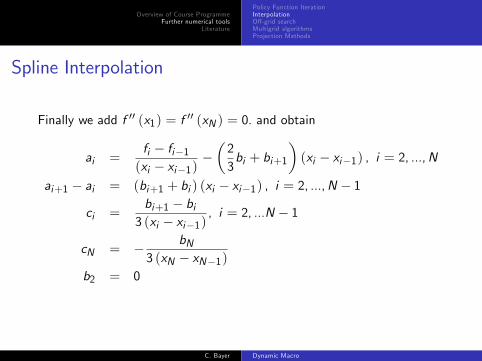
Spline Interpolation
Finally we add f ′′ (x1) = f ′′ (xN ) = 0. and obtain
ai =fi − fi−1(xi − xi−1)
−(23bi + bi+1
)(xi − xi−1) , i = 2, ...,N
ai+1 − ai = (bi+1 + bi ) (xi − xi−1) , i = 2, ...,N − 1
ci =bi+1 − bi3 (xi − xi−1)
, i = 2, ...N − 1
cN = − bN3 (xN − xN−1)
b2 = 0
C. Bayer Dynamic Macro

Overview of Course ProgrammeFurther numerical tools
Literature
Policy Function IterationInterpolationOff-grid searchMultigrid algorithmsProjection Methods
Spline Interpolation
While spline interpolation is very accurate, it is very time consuming if Nis large.
C. Bayer Dynamic Macro

Overview of Course ProgrammeFurther numerical tools
Literature
Policy Function IterationInterpolationOff-grid searchMultigrid algorithmsProjection Methods
Comparison of interpolation methods
0 1 2 3 4 5 6 7 80.5
1
1.5
2
2.5
3
3.5functionLS interpolationlinear interpolationspline interpolation
I Spline interpolation gives best results.I Linear interpolation is not bad either, yet, derivatives are constantbetween base points..
I With insuffi cient degrees of freedom, LS interpolation performsbadly.
C. Bayer Dynamic Macro

Overview of Course ProgrammeFurther numerical tools
Literature
Policy Function IterationInterpolationOff-grid searchMultigrid algorithmsProjection Methods
Off-grid search
I We can use interpolation methods to approximate dynamicprogramming problems.
I So far we considered approximations to the continuous state-spaceproblem
V (s) = maxy∈Γ(s)
u(s, s ′, ξ
)+ βV
(s ′).
by using a fine grid {s1, . . . , sN } for s and then solving by iteratingover the approximated, discretized problem.
Vn = max{U+ ιNV
n−1}.
C. Bayer Dynamic Macro

Overview of Course ProgrammeFurther numerical tools
Literature
Policy Function IterationInterpolationOff-grid searchMultigrid algorithmsProjection Methods
Off-grid search
Alternatively, we can define
V n (s) = Interpolation({V ni , si}i=1...N , s
)and update the base points, allowing for policies outside the grid{si}i=1...N .
V n+1i = maxy∈Γ(si )
u(si , s
′, ξ)+ βV n
(s ′)
C. Bayer Dynamic Macro

Overview of Course ProgrammeFurther numerical tools
Literature
Policy Function IterationInterpolationOff-grid searchMultigrid algorithmsProjection Methods
Off-grid searchExample
Exercise (13)Use the non-stochastic growth model with δ = 1.
1. Define a 10 point grid for k.
2. Use spline interpolation to solve for the value function, starting withV = 0 as initial guess, save running times.
3. Compare to the true value function at the grid points and noteaverage absolute difference.
4. Run a sequence of on-grid value function iterations withN = 10, 20, 40, 80, 160, 320 points. Compare average absolutedifference to the true model and running times with the off-gridsearch code.
C. Bayer Dynamic Macro

Overview of Course ProgrammeFurther numerical tools
Literature
Policy Function IterationInterpolationOff-grid searchMultigrid algorithmsProjection Methods
Chow and Tsitsiklis’(1991) Multigrid VFI
I We have seen that computation time for Value FunctionIteration as well as Policy Function Iteration grows polynomiallyin the number of grid points. (This can also been shown formallyusing complexity theory, see Rust (1996))
I Conversely this means that for small problems we can calculate thesolution relatively quickly.
C. Bayer Dynamic Macro

Overview of Course ProgrammeFurther numerical tools
Literature
Policy Function IterationInterpolationOff-grid searchMultigrid algorithmsProjection Methods
Chow and Tsitsiklis’(1991) Multigrid VFI
I Chow and Tsitsiklis (1991) suggest an algorithm that rests on thisinsight:
1. First solve the SDP on a sparse grid of points by VFI: This yields V ∗02. Increase the number of grid points in each dimension by factor 2.3. Obtain an initial guess V 01 for the value function on the new grid byinterpolation from the solution on the coarser grid.
4. Perform value function iteration to obtain V ∗1 for the enlarged grid.5. Repeat steps (2) to (4) until the grid is fine enough.
I Ideally the critical value for termination of the VFI decreases byfactor 2 in each grid iteration.
C. Bayer Dynamic Macro
Overview of Course ProgrammeFurther numerical tools
Literature
Policy Function IterationInterpolationOff-grid searchMultigrid algorithmsProjection Methods
Chow and Tsitsiklis’(1991) Multigrid VFI
I Chow and Tsitsiklis (1991) show that this algorithm almost reachesthe effi ciency bound (in terms of worst case complexity) foralgorithms to solve SDP.
I In practical applications the algorithm is linear in the number ofgridpoints.
I This does not hold true if VFI is to be replaced by PFI, becausecomplexity in the latter case stems from inverting the Policy matrix.
C. Bayer Dynamic Macro

Overview of Course ProgrammeFurther numerical tools
Literature
Policy Function IterationInterpolationOff-grid searchMultigrid algorithmsProjection Methods
Chow and Tsitsiklis’(1991) Multigrid VFI
I For practical purposes a mixed algorithm outperforms:I Use a multigrid PFI until the total number of gridpoints is about 500.I Then switch to VFI.
I One has to trade off grid generation time (e.g. Tauchen) againstmultigrid time saving.
I A further practical advantage of the multigrid algorithm comes indealing with outside loops: endogenous contracts, market clearingconditions, stationary equilibria etc.
I The following graphics compares computing times for the stochasticgrowth model:
C. Bayer Dynamic Macro

Overview of Course ProgrammeFurther numerical tools
Literature
Policy Function IterationInterpolationOff-grid searchMultigrid algorithmsProjection Methods
Comparison of running times
50 100 150 200 250 300 350 400 450 500 5500
5
10
15
20
25
30
35
number of grid points
runn
ing
time
[sec
]
VFIPFIMultigrid VFIMultigrid PFImixed Multigrid
VFI-Multigrid is linear, PFI-Multigrid is not!
C. Bayer Dynamic Macro

Overview of Course ProgrammeFurther numerical tools
Literature
Policy Function IterationInterpolationOff-grid searchMultigrid algorithmsProjection Methods
Multigrid VFI: Code
Switch to MATLAB, discuss code!
C. Bayer Dynamic Macro

Overview of Course ProgrammeFurther numerical tools
Literature
Policy Function IterationInterpolationOff-grid searchMultigrid algorithmsProjection Methods
Multigrid VFI: Exercises
Exercise (14a in class)Program a multigrid VFI algorithm to solve the stochastic income,consumption-savings problem using the simplified Tauchen procedure torepresent the AR-1 income process.
Exercise (14b)Extend the stochastic growth model such that utility is obtained from anaggregate of current and lagged consumption. Assume u (Ct ) = ln Ct
and Ct =(
αc−1t + (1− α) c−1t−1
)−1. Use a multigrid algorithm to solve
the model. Simulate the model! What effect does the change inpreferences have on the persistence of consumption? Compare the resultsfor α = 1, α = 0.8, α = 0.5. How can you interpret the model?
C. Bayer Dynamic Macro

Overview of Course ProgrammeFurther numerical tools
Literature
Policy Function IterationInterpolationOff-grid searchMultigrid algorithmsProjection Methods
Projection Methods
I All the before mentioned algorithms rely on the calculation of thevalue function to obtain the policy function, which is in mostapplications the object of interest.
I Projection methods directly solve for the policy function withoutsolving for the value function by invoking the Euler equation.
C. Bayer Dynamic Macro

Overview of Course ProgrammeFurther numerical tools
Literature
Policy Function IterationInterpolationOff-grid searchMultigrid algorithmsProjection Methods
Euler equation
I Consider a SDP
V (s) = maxc∈Γ(s)s ′=f (s ,c )
u (c) + βEV(s ′)
I The first order condition is
u′ (c) + βEV ′(s ′)f ′c (s, c) = 0
I Optimality (envelope theorem) implies
V ′ (s) = βEV ′(s ′)f ′s (s, c)
C. Bayer Dynamic Macro

Overview of Course ProgrammeFurther numerical tools
Literature
Policy Function IterationInterpolationOff-grid searchMultigrid algorithmsProjection Methods
Euler equation
I Therefore first order condition is
u′ (c)f ′s (s, c)f ′c (s, c)
= −V ′ (s)
I Plugging this back in yields the Euler equation
u′ (c) = βE(u′(c ′)f ′s(s ′, c ′
))I The optimal policy trades off marginal utility today and discountedexpected marginal utility tomorrow, taking into account the relativemarginal effect of c and s on the future state s ′.
C. Bayer Dynamic Macro

Overview of Course ProgrammeFurther numerical tools
Literature
Policy Function IterationInterpolationOff-grid searchMultigrid algorithmsProjection Methods
Projection methods
I Projection methods exploit the Euler equation
u′ (c)− βE(u′(c ′)f ′s(s ′, c ′
))= 0
I Define the policy function c = h (s), then we can rewrite the Eulerequation as
Fh (s) := u′ (h (s))
− βE(u′ (h (f (s, h (s)))) f ′s (f (s, h (s)) , h (f (s, h (s))))
)= 0
C. Bayer Dynamic Macro

Overview of Course ProgrammeFurther numerical tools
Literature
Policy Function IterationInterpolationOff-grid searchMultigrid algorithmsProjection Methods
Projection methods
I Projection methods parametrize h, for example by a Chebyshevpolynomial.
h (s) =n
∑i=1
ψi ci (xi )
and we need to determine ψi , i = 1, ..., n.I Ideally the base functions should look alike the policy function.I We cannot expect Fh (s) = 0 for all s.I Therefore we minimize ||Fh || for some appropriate metric ||·||.I The metric is from the class ||F || =
∫A F (a) g (a) da, where g is
some weighting function
C. Bayer Dynamic Macro

Overview of Course ProgrammeFurther numerical tools
Literature
Policy Function IterationInterpolationOff-grid searchMultigrid algorithmsProjection Methods
Least square metric
I One possible metric is the least square metric.I This leads to the minimization problem
minψ
∫ [Fh (s)
]2 dsI The integral has to be solved numerically
C. Bayer Dynamic Macro

Overview of Course ProgrammeFurther numerical tools
Literature
Policy Function IterationInterpolationOff-grid searchMultigrid algorithmsProjection Methods
Collocation method
I An alternative metric uses the mass point function as weighting.I This function takes value 1 if x = xi for a pre-specified set of points.I If one uses n points, the ψi become exactly identified and thereforethe collocation method forces Fh to be exactly zero at xi .
I Ideally one chooses xi as the roots of the base functions, i.e. forChebyshev polynomials xi = cos
(π2i
).
I So that we obtain a system of n equations Fh (xi ) = 0 which is tobe solved for ψ.
C. Bayer Dynamic Macro

Overview of Course ProgrammeFurther numerical tools
Literature
Policy Function IterationInterpolationOff-grid searchMultigrid algorithmsProjection Methods
Exercise
Exercise (15)Derive the Euler equation for the consumption model with u = c1−γ−1
1−γ ,fluctuating income and a constant interest rate R. Reformulate the Eulerequation such that you obtain an expression of the formEt (g (ct , ct+1)) = 0. Define εt+1 := g (ct , ct+1) , what can you tellabout the correlation of εt+1 and variables that are perfectly observed attime t?
C. Bayer Dynamic Macro

Overview of Course ProgrammeFurther numerical tools
Literature
LiteraturePrimary Reading:I Heer, B. and A. Maussner (2009), "Dynamic General EquilibriumModelling", 2nd edition, Springer, Berlin. (Ch. 11)
I Adda, J. and R. Cooper (2004): "Dynamic Economics", MIT Press,Cambridge (Ch. 3)..
Secondary reading:I Chow, C.S. and J.N. Tsitsiklis (1991): "An optimal multigrid algorithmfor continuous state discrete time stochastic control", IEEE Transactionson Automatic Control, 36(8), 898—914.
I Ljungqvist, L. und T. Sargent (2004): "Recursive MacroeconomicTheory", MIT press, Cambridge.
I Stockey, N.L. and Lucas, R.E. with E.C. Prescott (1989): "RecursiveMethods in Economic Dynamics", Chapters 4 and 9, HUP, Cambridge.
I Sundaram R. K. (1996): "A first course in Optimization Theory",Chapters 11 and 12, CUP, Cambridge.
I Tauchen, G. (1986): "Finite state Markov-chain approximation tounivariate and vector autoregressions", Economic Letters, 20, 177-81.
C. Bayer Dynamic Macro

Overview of Course ProgrammeEstimation
Simulation based estimationLiterature
Part 4Estimation
C. Bayer Dynamic Macro

Overview of Course ProgrammeEstimation
Simulation based estimationLiterature
Programme of this week
1. Discussing the Exercises
2. Non-Simulation Based Estimation
2.1 Maximum Likelihood2.2 Generalized Methods of Moments
3. Simulation Based Estimation
3.1 Bootstrap3.2 Indirect Inference and method of simulated moments
C. Bayer Dynamic Macro

Overview of Course ProgrammeEstimation
Simulation based estimationLiterature
Maximum LikelihoodGMM Estimation
Estimation
I In general we do not directly observe the parameters of the model,but for any numerical analysis we need to fix parameters to certainvalues.
I In doing so we want to obtain a maximal fit of our model with thedata.
I At the same time, we want to evaluate how likely it is that the datawhich we observe is actually generated by our model.
I First we’ll go through some more standard estimation techniquesbefore we discuss particular techniques to estimate numerical models.
C. Bayer Dynamic Macro

Overview of Course ProgrammeEstimation
Simulation based estimationLiterature
Maximum LikelihoodGMM Estimation
Maximum Likelihood
I The most effi cient - though not always feasible - classical estimationmethod is maximum likelihood estimation.
I It is a prerequisite for this method that we exactly know thedistribution of shocks that drive our model.
I However this is typically not a problem, since we needed to assumesome distribution anyway in order to solve the model.
C. Bayer Dynamic Macro

Overview of Course ProgrammeEstimation
Simulation based estimationLiterature
Maximum LikelihoodGMM Estimation
Maximum Likelihood
I Let εt , t = 1...T be a sequence of i.i.d. shocks, Xt be the sequenceof states, and Yt be the sequence of policy variables generated fromour model.
I Then we can view the model as some data generating process Φthat generates a sequence
[X , Y ]t = Φ (Xt−1, εt |θ)
I Maximum likelihood estimation rests on the inversion of Φ("backing out the shocks") for given model parameters θ.
C. Bayer Dynamic Macro

Overview of Course ProgrammeEstimation
Simulation based estimationLiterature
Maximum LikelihoodGMM Estimation
Conditional Maximum Likelihood: algorithm
I Typically we start with some X0, ε0 and then recursively obtain anerror estimate
εt (θ) = Φ−1 (Xt ,Yt |Xt−1, θ, εt−1)
I Then we obtain the likelihood function as
L ({εt (θ)}t=1...T ) =T
∏t=1
f (εt (θ))
I We then maximize L by choosing θ
C. Bayer Dynamic Macro

Overview of Course ProgrammeEstimation
Simulation based estimationLiterature
Maximum LikelihoodGMM Estimation
Maximum Likelihood: 2 issues
I The first problem that we may encounter, is that F is not invertible.Therefore there is no one-to-one mapping that maps shocks tostates.
I In other words, under our model one sequence of states of naturemay be a result of various sequences of shocks.
I In this case the two series of shocks are said to be observationallyequivalent and the model is not identified.
C. Bayer Dynamic Macro

Overview of Course ProgrammeEstimation
Simulation based estimationLiterature
Maximum LikelihoodGMM Estimation
Maximum Likelihood: 2 issues
I The other issue is less of a problem from a scientific point of view,though of terrible importance to the researcher: thezero-probability problem
I It may be that F is invertible, but under all admissible modelparameters the sequence (X Y )t cannot be generated by arbitraryshocks.
I In this case the model is simply wrong. E.g. assume you supposext = 1
1+θ exp(εt ). If you observe some x /∈ (0, 1) then the model
must be wrong and is to be rejected.I Zero probability is a degenerated case of model rejction due to lowprobability of observing the data even under the most favourablechoice of θ.
C. Bayer Dynamic Macro

Overview of Course ProgrammeEstimation
Simulation based estimationLiterature
Maximum LikelihoodGMM Estimation
Maximum Likelihood: An exampleI Consider flipping a coin that has probability θ to show heads andtails otherwise.
I Suppose we observe N1 times heads out of N draws.I Then the Likelihood function is
L (x , θ) = θN1 (1− θ)N−N1
ln L = N1 ln θ + (N −N1) ln (1− θ) .
I Maximization leads to
N11θ− (N −N1)
11− θ
= 0
θ∗ =N1N
C. Bayer Dynamic Macro

Overview of Course ProgrammeEstimation
Simulation based estimationLiterature
Maximum LikelihoodGMM Estimation
Maximum Likelihood: Estimation of the capitalaccumulation model
I Suppose we want to estimate the production function parameter α,the shock process parameters ρ and σ from our growth model. Weassume a log-normal AR-1 process for productivity.
I Fix β = 0.95, δ = 0.05 and µ = 0.I We use German NAICS data on consumption and investment inlogs, detrended and demeaned. We assume Y = C + I and use thisvariable for inference, i.e. we back-out the shocks that exactlyreproduce the output series.
I We fix k0 to the steady state value at mean productivity. And dropthe first 10 quarters of the residual to minimize the influence of theinitial choice of k.
I Switch to MATLAB!
C. Bayer Dynamic Macro

Overview of Course ProgrammeEstimation
Simulation based estimationLiterature
Maximum LikelihoodGMM Estimation
Maximum Likelihood: Model comparison
I By itself ML Estimation can only perform a weak test of thequalities of the model.
I It only tells us, whether the observed data can be generated by themodel and some sequence of shocks even if this sequence has anarbitrary small likelihood.
I Standard approaches to model comparison such as LR tests onlywork in nested models, e.g. we can test a risk aversion of oneagainst alternative CRRA formulations.
I Test approaches such as Vuong (1989) tests (similar to AIC) arebetter suited, they allow to compare our theoretical model to anatheoretical descriptions of the data, such as (V)ARs.
C. Bayer Dynamic Macro
Overview of Course ProgrammeEstimation
Simulation based estimationLiterature
Maximum LikelihoodGMM Estimation
GMM Estimation
I A downside of the ML Estimation is usually that we need to knowthe distribution of the shocks ε to the economic system.
I Generalized method of moments estimation evades this problem byrelying only on information on a number of moments generated by εand our model.
I This also has computational advantages, because "backing out theshocks" can be quite computational intense.
I Note that GMM only helps if we can derive the moment conditionsfrom theory, because moment conditions need to hold exactly.
C. Bayer Dynamic Macro

Overview of Course ProgrammeEstimation
Simulation based estimationLiterature
Maximum LikelihoodGMM Estimation
GMM Estimation
I Suppose Mθ is the set of all moments generated by our model underthe parameter choice θ. Let µ (θ) be a subset of these moments thatis used for the estimation.
I Let θ be the true parameters that nature has chosen.I If our model is correct, then
E(µ(θ)− µ
(θ))= 0
where µ is the sample analogue to µ.
I Define g (xt , θ) as the moment generating function andF (xt , θ) = g (xt , θ)− µ (θ) .
C. Bayer Dynamic Macro

Overview of Course ProgrammeEstimation
Simulation based estimationLiterature
Maximum LikelihoodGMM Estimation
GMM Estimation
I We can use this observation to construct an estimation procedure.I Suppose E (F (x , θ)) = 0 has a unique solution, then this is θ.
I If we have as many moments as parameters (exact identification),we obtain
θ = µ−1 (µ) .
I Typically we will choose more moments than parameters, since
1. this increases effi ciency if the moments are informative (i.e. notconstant in θ, not collinear to other moments)
2. this allows us to construct a test of our model
C. Bayer Dynamic Macro

Overview of Course ProgrammeEstimation
Simulation based estimationLiterature
Maximum LikelihoodGMM Estimation
GMM Estimation
I If we have more moments than parameters (overidentification), weminimize the quadratic expression
θ = argmin (FT (x , θ))W (FT (x , θ))′
I Where FT are the sample means of F and W is a weighting matrixthat ideally takes into account the variance-covariance structure ofFT and gives large weight to those moments that are estimated withhigh precision.
C. Bayer Dynamic Macro

Overview of Course ProgrammeEstimation
Simulation based estimationLiterature
Maximum LikelihoodGMM Estimation
GMM EstimationI Let fT be the average derivative of FT in the sample, i.efT (θ) =
1T ∑Tt=1
∂F (xt ,θ)∂θ .
I Then the estimator
θ = argminFT (θ)WFT (θ)′
is asymptotically normally distributed and has a variance of(f ′TWfT
)−1 (f ′TWVTWfT ) (f ′TWfT )−1I where VT is the long run variance of FT (θ) .
VT = E
( T
∑t=1
F (xt , θ)
)2C. Bayer Dynamic Macro

Overview of Course ProgrammeEstimation
Simulation based estimationLiterature
Maximum LikelihoodGMM Estimation
GMM Estimation
I This means the optimal choice for W is V−1T , which confirms ourinitial guess.
I Calculating V−1T is complicated in most cases, because this involvesθ.
I If moment conditions are formulated such that g does not depend onθ, a single bootstrap procedure provides us with an estimate of VT .
I Otherwise it is one possible algorithm to obtain an estimate of V tostart with any initial pds weighting matrix W and then update Witeratively using some appropriate method to estimate V .
I There is a number of alternatives to do so, see Matyas (1999) forexample. Examples are HAC, Newey-Whited or Bootstrapestimation procedures.
C. Bayer Dynamic Macro

Overview of Course ProgrammeEstimation
Simulation based estimationLiterature
Maximum LikelihoodGMM Estimation
GMM Estimation: Example 1
I Consider again the coin-flipping example.I Say heads has value one and tails zero.I Then the expected value of x is θ.
I Moreover the variance of x is var (x) = θ (1− θ)
C. Bayer Dynamic Macro

Overview of Course ProgrammeEstimation
Simulation based estimationLiterature
Maximum LikelihoodGMM Estimation
(G)MM Estimation: Example 1I However the second moment is not informative. Whenever the firstmoment condition is met, then also the second moment conditionholds.
I Therefor the MM estimator is
argmin(N1N− θ
)2I FOC
−2(N1N− θ
)= 0
θ∗ =N1N
I Which is actually the ML estimate
C. Bayer Dynamic Macro

Overview of Course ProgrammeEstimation
Simulation based estimationLiterature
Maximum LikelihoodGMM Estimation
GMM Estimation: Example 2
I Suppose, we have the linear regression model
yt = Xtβ+ ut
I Where dim(Xt ) = p, cov(Xt , ut ) 6= 0 but there is some Zt withdim(Zt ) = q and rk (E (Z ′Z )) = q and cov(Zt , ut ) = 0.
I If further X and Z are not orthogonal, we can formulate as momentcondition
E(Z ′t (yt − Xtβ)
)= 0
F (β) =1T ∑Z ′t (yt − Xtβ) =
1TZ ′ (y − X β)
C. Bayer Dynamic Macro

Overview of Course ProgrammeEstimation
Simulation based estimationLiterature
Maximum LikelihoodGMM Estimation
GMM Estimation: Example 2
I Then with cov(u) = σ2I
V =1TZ ′ (y − X β)
(Z ′ (y − X β)
)′=
1TZ ′uu′Z
=1T ∑
(Z ′tututZt
)= σ2T−1Z ′Z
I And f (β) = Z ′X
C. Bayer Dynamic Macro

Overview of Course ProgrammeEstimation
Simulation based estimationLiterature
Maximum LikelihoodGMM Estimation
GMM Estimation: Example 2
I Therefore the GMM estimator becomes
β = argmin1TZ ′ (y − X β)
(Z ′Z
)−1 (y ′ − β′X ′)Z
β =(X ′Z
(Z ′Z
)−1 Z ′X)−1 X ′Z (Z ′Z)−1 Z ′yI which is the IV estimator with more instrumental than modelvariables.
C. Bayer Dynamic Macro

Overview of Course ProgrammeEstimation
Simulation based estimationLiterature
Maximum LikelihoodGMM Estimation
GMM Estimation: Testing overidentifying restrictions
I To perform a test of the model in the GMM framework, we test howclose
QT = FT(θ)WFT
(θ)′
actually gets to zero.I Under the condition that W = V−1T Hansen (1982) shows that
JT = TQT
is χq−p distributed, where q is the number of linear independentmoment restrictions and p is the number of parameters.
C. Bayer Dynamic Macro

Overview of Course ProgrammeEstimation
Simulation based estimationLiterature
Bootstrap estimation of Variance Covariance structuresIndirect inference and the method of simulated moments
Simulation based estimation
I Both Maximum likelihood estimation and the generalized method ofmoments have serious drawbacks in the estimation of dynamicmodels.
I For GMM we have to rest on analytical results,I ML-Estimation quickly becomes numerically infeasible, involving thesolution of multiple integrals and so on.
I Simulation based estimation methods are the “natural”way to thinkabout estimation of numerical models.
C. Bayer Dynamic Macro

Overview of Course ProgrammeEstimation
Simulation based estimationLiterature
Bootstrap estimation of Variance Covariance structuresIndirect inference and the method of simulated moments
Simulation based estimation
I We will focus on the method of simulated moments and itsextension to indirect inference
I These methods can be thought of as extensions of GMMI or as “calibration with confidence bounds”
C. Bayer Dynamic Macro

Overview of Course ProgrammeEstimation
Simulation based estimationLiterature
Bootstrap estimation of Variance Covariance structuresIndirect inference and the method of simulated moments
Bootstrap estimates of the variance covariance structure
I Suppose we observe a data sample xt , t = 1...T .I We are interested in some expression of the form γ (X ) ∈ Rn and itsdistribution, for example sample moments.
I Not always can we determine the covariance structure of γ fromanalytical grounds without knowing the distribution of X .
I Bootstrapping can help in this situation.
C. Bayer Dynamic Macro

Overview of Course ProgrammeEstimation
Simulation based estimationLiterature
Bootstrap estimation of Variance Covariance structuresIndirect inference and the method of simulated moments
Bootstrap estimates of the variance covariance structure
I We resample N artificial samples Xi from X by drawing T timesfrom X with replacement.
I This gives a sample of i = 1...N realizations γi of which we caneasily determine the variance structure in sample.
I For T → ∞ and N → ∞ the bootstrap sample variance convergesto the theoretical variance.
I For example in GMM Estimation this is useful to estimate thevariance matrix of moments.
C. Bayer Dynamic Macro

Overview of Course ProgrammeEstimation
Simulation based estimationLiterature
Bootstrap estimation of Variance Covariance structuresIndirect inference and the method of simulated moments
Exercise
Exercise (16)Write a programme that
1. Simulates the VAR(y1y2
)t= B
(y1y2
)t−1
+
(ε1ε2
)t, B =
[0.7 0.1−0.2 0.6
]for T=200 periods where ε ~N(0, I ) .
2. Estimates B with OLS
3. Draws N=1000 Bootstrap samples
4. Re-estimates B with OLS for each of the samples.
5. Compares the standard deviation from the estimate of the bootstrapsamples and the standard error derived from asymptotic theory ofthe estimate from the simulated sample.
C. Bayer Dynamic Macro

Overview of Course ProgrammeEstimation
Simulation based estimationLiterature
Bootstrap estimation of Variance Covariance structuresIndirect inference and the method of simulated moments
Method of simulated moments
I The method of simulated moments (MSM) builds upon the idea ofmoment-matching in GMM estimation.
I However, what is compared in the MSM case are moment estimatesfrom Monte-Carlo simulations of our economic model and observeddata moments.
I Let yt , t = 1...T be a sequence of observations which we suppose tobe generated by the economic model Φ.
I Let g (yt , yt−1, ..., yt−l ) ∈ Rk be the moment generating functionthat exploits information from up to l lags of y .
C. Bayer Dynamic Macro

Overview of Course ProgrammeEstimation
Simulation based estimationLiterature
Bootstrap estimation of Variance Covariance structuresIndirect inference and the method of simulated moments
Method of simulated moments
I We draw R independent (Monte Carlo) simulations of our model togenerate simulated datasets y rt (θ) , t = 1...T , r = 1...R.
I The length of T is the same as in the sample of observations.I Typically we need to define a starting state for the model y0.
I If possible this is taken as a random draw from the ergodicdistribution of y under Φ (θ) .
I If this is not feasible, we can choose a sensible starting value y−τ andthen simulate the model for some additional initial periods τ whichwe then drop.
I We estimate the moments implied by the model as
µ (θ) := R−1 (T − l)−1R
∑r=1
T
∑t=lg(y rt (θ) , y
rt−1 (θ) , ..., y
rt−l (θ)
)
C. Bayer Dynamic Macro

Overview of Course ProgrammeEstimation
Simulation based estimationLiterature
Bootstrap estimation of Variance Covariance structuresIndirect inference and the method of simulated moments
Method of simulated moments
I The MSM estimate then is
θMSM := argmin (µ− µ (θ))W (µ− µ (θ))′
I where W is some pds matrix.I Ideally we use W = V−1 where V is the var(µ− µ (θ)) ,approximated by var(µ) .
C. Bayer Dynamic Macro

Overview of Course ProgrammeEstimation
Simulation based estimationLiterature
Bootstrap estimation of Variance Covariance structuresIndirect inference and the method of simulated moments
Method of simulated moments
I In this case Duffi e and Singleton (1993) show that
T12(θMSM − θ0
) d→ N(0,(1+ R−1
) (DV−1D
)−1)where
D = E∂µ (θ0)
∂θ
I This means that the MSM estimator is only by a factor(1+ R−1
)less effi cient than the GMM estimator.
I Already for relative small values of R, e.g. R = 5 or R = 10, theloss in precision is mild.
C. Bayer Dynamic Macro

Overview of Course ProgrammeEstimation
Simulation based estimationLiterature
Bootstrap estimation of Variance Covariance structuresIndirect inference and the method of simulated moments
Choice of Moments
I From the inspection of the formula of the asymptotic variance of theMSM estimator
avar(θMSM
)=(1+ R−1
) (DV−1D
)−1we can see that the precision of the estimate will crucially depend onthe sensitivity of moments to model parameters.
I If moments only weakly depend on model parameters, then D issmall and the estimate will be imprecise.
I In small samples the choice of overly many moments can lead to asubstantial effi ciency loss.
C. Bayer Dynamic Macro

Overview of Course ProgrammeEstimation
Simulation based estimationLiterature
Bootstrap estimation of Variance Covariance structuresIndirect inference and the method of simulated moments
Choice of Moments
I This means from an econometric point of view we should choosemoments which are very informative as they depend strongly onmodel parameters and are also estimated with little uncertainty(small V ).
I However, if we loosen the econometric point of view somewhat, thenwe can also understand the choice of the set of moments as aparticular point of view from which we analyze the model.
I This second view tends more towards the practice in calibration,where we choose a set of moments which we feel is essential forthe model to match in the light of its economic content.
C. Bayer Dynamic Macro

Overview of Course ProgrammeEstimation
Simulation based estimationLiterature
Bootstrap estimation of Variance Covariance structuresIndirect inference and the method of simulated moments
Moments and indirect inference
I The MSM estimation can be extended to the use of regressioncoeffi cients as moments.
I For this purpose, we define an auxiliary mispecified model Φ∗ todescribe the data in reduced form.
I This model has a parameter vector β with q ≥ p parameters.I We can use the parameter estimates β as moments and use asweighting matrix their variance covariance structure implied by theestimation procedure used to estimate β assuming Φ∗ were actuallycorrect.
C. Bayer Dynamic Macro

Overview of Course ProgrammeEstimation
Simulation based estimationLiterature
Bootstrap estimation of Variance Covariance structuresIndirect inference and the method of simulated moments
Indirect inferenceI If we estimate β by quasi maximum likelihood, then this is theindirect inference proposed by Monfort et al. (1993), akasimulated minimum distance estimator.
I Galant and Tauchen (1996) suggest an alternative indirect inferenceprocedure
I that minimizes a qudratic form of the score functions (derivatives ofthe log-likelihood) of the auxiliary model,
I using the simulated data and the parameter estimate from theauxiliary model and the observed data.
I The optimal weighting matrix is the variance of the scores.
I Smith (1993) suggests a third alternative: simulated quasi maximumlikelihood, in which
I the likelihood of the observed data under the auxiliary model ismaximized
I imposing the ML parameter estimates from the auxiliary model underthe simulated data
C. Bayer Dynamic Macro

Overview of Course ProgrammeEstimation
Simulation based estimationLiterature
Bootstrap estimation of Variance Covariance structuresIndirect inference and the method of simulated moments
Effi cient method of moments
I A particular advantage of the indirect inference formulation is thatthe auxiliary model can be chosen data dependent.
I If we increase the complexity of the auxiliary model with T(increasing q, using a semiparametric auxiliary model) the Galantand Tauchen Estimator approaches asymptotically the effi ciencybound. (i.e. is equivalent to the infeasible ML of Φ)
I This estimator is termed Effi cient method of moments (EMM).I However, it may behave poorly in small samples.
C. Bayer Dynamic Macro

Overview of Course ProgrammeEstimation
Simulation based estimationLiterature
Bootstrap estimation of Variance Covariance structuresIndirect inference and the method of simulated moments
MSM: Estimation of the capital accumulation model
I Suppose we want to estimate the production function parameter α,risk aversion γ and the shock process parameters ρ and σ from ourgrowth model. We assume a log-normal AR-1 process forproductivity.
I We fix β = 0.95, δ = 0.05 and µ = 0.I We use German quarterly NAICS data on consumption andinvestment in logs, detrended and demeaned. We assumeY = C + I .
I We fix k0 to the steady state value at mean productivity and dropthe first 10 years of the simulation to minimize the influence of theinitial choice of k.
I We use as moments the standard deviations σY , σI , and the firstorder autocorrelations ρY , ρI .
I Switch to MATLAB!
C. Bayer Dynamic Macro

Overview of Course ProgrammeEstimation
Simulation based estimationLiterature
LiteraturePrimary Reading:
I Adda, J. and R. Cooper (2004): "Dynamic Economics", MIT Press,Cambridge (Ch. 4)..
Secondary reading:
I Matyas, L. (1999): "Generalized Method of Moments Estimation", CUP,Cambridge, Ch. 1-3. & 10.
I Gourieroux, C., A. Monfort, and E. Renault (1993): "Indirect inference",Journal of Applied Econometrics, 8, p. 85-118.
I Smith, T. (1993): "Estimating nonlinear time-series models usingsimulated vector autoregressions", Journal of Applied Econometrics, 8, p.63-84.
I Vuong, Q. H. (1989): "Likelihood Ratio Tests for Model Selection andNon-Nested Hypotheses," Econometrica, 57, 307 - 333.
C. Bayer Dynamic Macro

Overview of Course ProgrammeFurther theoretical elements in dynamic economics
Part 5General equilibrium,
Semi-strategic interactions,Dynamic Games
C. Bayer Dynamic Macro

Overview of Course ProgrammeFurther theoretical elements in dynamic economics Numerical Tools
Programme of this Part
1. Discussion of Exercises
2. General Equilibrium
3. Incorporating zero profit conditions
C. Bayer Dynamic Macro

Overview of Course ProgrammeFurther theoretical elements in dynamic economics
General equilibrium (Decentralization)Zero Profit ConditionsStrategic Interactions
General equilibrium(Decentralization, recursive equilibrium)
I Suppose we model an economy in a dynamic setup, in which someor all actions of economic agents are described as infinite horizondynamic programming problems.
I If all agents are alike (or of a finite number of types), then we candescribe the economy by an aggregate state vector S .
I The agents take the evolution H (S) as given (general equilibrium).I Prices depend on the aggregate state P (S) .
C. Bayer Dynamic Macro

Overview of Course ProgrammeFurther theoretical elements in dynamic economics
General equilibrium (Decentralization)Zero Profit ConditionsStrategic Interactions
Recursive equilibrium
DefinitionA recursive equilibrium is comprised of
I price functions P (S) ,I individual policy functions h (s, S) that solve the dynamicprogramming problem,
I a law of motion H (S) for the aggregate economy,such that
I all agents optimize taking P and H as givenI markets clearI and the aggregate law of motion and the individual policy functionsare consistent, i.e. H (S) = h (S , S) .
C. Bayer Dynamic Macro

Overview of Course ProgrammeFurther theoretical elements in dynamic economics
General equilibrium (Decentralization)Zero Profit ConditionsStrategic Interactions
Example: Capital accumulationI Suppose we extend the capital accumulation model, such thathouseholds and firms are separated.
I Capital is held by households which rent it out to the firm sectorthat is owned by the households.
I The households planning problem is
V (k,A,K ) = maxk ′u((r (K ) + (1− δ)) k − k ′ +Π
)+ βEV
k ′, A′,K ′︸ ︷︷ ︸=H (A,K )
I Competitive capital and product markets are characterized by
r (K ) k = αzkα
Π = (1− α) zkα
C. Bayer Dynamic Macro

Overview of Course ProgrammeFurther theoretical elements in dynamic economics
General equilibrium (Decentralization)Zero Profit ConditionsStrategic Interactions
Solution strategies
1. Often the recursive equilibrium can be shown to be the solution of acentral planner problem, which can be solved using standardtechniques.
2. Alternatively, we begin with a guess of H and P and iterate untilconvergence. Note, however, that the dimensionality of the problemincreases and we need an outside loop to find H and P. Finally,convergence is not guaranteed.
C. Bayer Dynamic Macro

Overview of Course ProgrammeFurther theoretical elements in dynamic economics
General equilibrium (Decentralization)Zero Profit ConditionsStrategic Interactions
Zero Profit Conditions
I Consider a situation in which two agents interact and one agentoffers a contract r (s) to the other agent.
I The agent offering the contract is bound by a zero profit condition,but has to take the actions of the other agents into account.
I Generically we can write the situation as
Vr (s) = maxs ′∈Γ(s)
u(s, s ′|r (s)
)+ βEVr
(s ′)
with φ being the associated policy and r being implicitly defined by
π (r (s) , φr (s)) = 0
C. Bayer Dynamic Macro

Overview of Course ProgrammeFurther theoretical elements in dynamic economics
General equilibrium (Decentralization)Zero Profit ConditionsStrategic Interactions
Zero Profit conditions
I We need to find an optimal policy function (strategies) of thedecision maker given r .
I And r has to fulfill the zero-profit condition, given the policyfunction φ.
I Therefore one possible way to solve the problem is to assume afunction r0, then find the optimal φ1 for this guess, then update r tor1 and so on.
I This does not necessarily converge.
C. Bayer Dynamic Macro

Overview of Course ProgrammeFurther theoretical elements in dynamic economics
General equilibrium (Decentralization)Zero Profit ConditionsStrategic Interactions
Exercise 17Debt contracts
Exercise (17)Extend the consumption model such that the agent can decide to defaulton his obligations. In the case of default, the agent surrenders all hiswealth and future income except for the fixed income τ income to hiscreditors. There is perfect competition among creditors who themselvesborrow at rate R. Assume that in case of bankruptcy, in addition to theloss in the debt claim, the creditor also loses some fixed amount κ toacquire the debtors income.
C. Bayer Dynamic Macro

Overview of Course ProgrammeFurther theoretical elements in dynamic economics
General equilibrium (Decentralization)Zero Profit ConditionsStrategic Interactions
Strategic interactions
I So far we studied situations with little or no interaction of economicentities.
I Real economic situations often involve strategic interactions.I These become quickly infeasible to study in terms of DP.I However, we want to lay out the principles of such analysis.
C. Bayer Dynamic Macro

Overview of Course ProgrammeFurther theoretical elements in dynamic economics
General equilibrium (Decentralization)Zero Profit ConditionsStrategic Interactions
Strategic interactions
I To be able to model a strategic interaction in a dynamic context, wefirst need to adapt the problem to a multi-decsionmaker setup.
I Let s be the total state vector whereas si is the state vector undercontrol by decision maker i . Let S and Si be the correspondingchoice sets.
I Suppose pi (s) = s ′i defines the perceived policy function forindividual i - perceived by its competitors.
I We can state the individual optimization problem as
Vi (si , s−i ) = maxs ′i ∈Si
u(si , s−i , s
′i , p−i (s)
)+ βEVi
(s ′i , p−i (s)
)
C. Bayer Dynamic Macro

Overview of Course ProgrammeFurther theoretical elements in dynamic economics
General equilibrium (Decentralization)Zero Profit ConditionsStrategic Interactions
Strategic interactions
DefinitionA Markov perfect equilibrium, now is a set of perceived policyfunctions pi , Value Functions Vi and actual Policy Functions Pi such that
1. given p−i , the Value Function Vi and the corresponding PolicyFunctions Pi solve the agents optimization problem.
2. Pi = pi for all i .
Remark: The recursive formulation incorporates the Markov property:Policies only condition on the state and not on the entire history of thegame. Perfectness is included by defining policies for each possible state,regardless whether this state is reached in equilibrium or not.
C. Bayer Dynamic Macro

Overview of Course ProgrammeFurther theoretical elements in dynamic economics
General equilibrium (Decentralization)Zero Profit ConditionsStrategic Interactions
Strategic interactions: Solution strategy
I While the formulation looks straightforward, finding a solutionbecomes quickly infeasible. Moreover it is often not clear in advancewhether a solution exists.
I Often the following algorithm succeeds in finding the equilibrium:
1. Start with some initial guess for the policy functions of p0i .2. Find the optimal policy p1i for each i under the assumption thatp−i = p0−i .
3. Iterate until convergence.
C. Bayer Dynamic Macro

Overview of Course ProgrammeFurther theoretical elements in dynamic economics
General equilibrium (Decentralization)Zero Profit ConditionsStrategic Interactions
Strategic interactions: Solution strategy
I While in practice such algorithm may succeed, one can easily seethat it does not necessarily do so by considering the static analogueto this algorithm.
I The idea behind this algorithm is to define T (si ) = Ri (R−i (si ))and construct a sequence sni = T
n (si ) , where Ri is the bestresponse function.
I If T is a contraction, the algorithm succeeds and finds the uniqueequilibrium.
I However, there may be more than one equilibrium, or the sequencemay actually diverge: Suppose
Ri (s−i ) = a+ bs−i
If b > 1 then the sequence will diverge.
C. Bayer Dynamic Macro

Stationary heterogeneous agent economies
Part 6Stationary heterogeneous agent economies
C. Bayer Dynamic Macro

Stationary heterogeneous agent economiesIntroductionHuggett’s modelAiyagari’s model
Heterogeneous agent economies
I A further complication arises if economies consist of heterogeneousagents, like households differing in their wealth levels and havingnon-linear consumption functions. Our definition of a recursiveequilibrium relied on the assumption of a single (type) of consumeror firm.
I However, if one takes the statement of heterogeneous agentsseriously, an exact analysis becomes infeasible.
I Suppose there is a continuum of consumers, all indexed by theirwealth level W . The distribution of wealth across consumers shall becharacterized by density µ (W ) .
C. Bayer Dynamic Macro

Stationary heterogeneous agent economiesIntroductionHuggett’s modelAiyagari’s model
Heterogeneous agent economies: The Problem
I In such economy, aggregate demand will in general depend on thedistribution of wealth µ (W ) .
I Therefore also prices depend on the distribution of wealthp = p (·, µ (W )) .
I This, however, means that the whole distribution µ is a state of theeconomy.
I Yet, µ is an infinite dimensional object and hence not numericaltractable.
C. Bayer Dynamic Macro

Stationary heterogeneous agent economiesIntroductionHuggett’s modelAiyagari’s model
Heterogeneous agent economies: Stationary economies
I One way to circumwent these problems is to look at economieswithout aggregate fluctuations.
I In such economies, prices are constants.I Although they depend on µ, this dependence does not matter.I Next we consider such models.
C. Bayer Dynamic Macro

Stationary heterogeneous agent economiesIntroductionHuggett’s modelAiyagari’s model
A particular savings problem
I Suppose income can take m levels yi .I For an individual household yt evolves according to a Markov Chainwith transition probability Π.
I [a special case is two states: unemployed y0 = b and employedy1 = 1].
I The household can hold assets in amounts given by a gridA = {a1, . . . , an} , where aj−1 < aj , 0 ∈ A.
C. Bayer Dynamic Macro

Stationary heterogeneous agent economiesIntroductionHuggett’s modelAiyagari’s model
A particular savings problem
I The household chooses ct (and thus at ) in order to maximize
E0∞
∑t=0
βtu (ct )
s.t. ct + at+1 = (1+ r) at + yt ; at+1 ∈ A
I We can treat prices as time-fixed, because we just want to look atthe steady-state distribution of assets, when the cross-sectionaldistribution of s and a is its ergodic distribution.
I We assume that β (1+ r) < 1, which is no real restriction sinceotherwise no stationary equilibrium exists.
C. Bayer Dynamic Macro

Stationary heterogeneous agent economiesIntroductionHuggett’s modelAiyagari’s model
A particular savings problem
I The Bellman equation is
V (ah , yi ) = maxa′∈A
u((1+ r) ah + yi − a′
)+ β
m
∑j=1
Π (i , j) v(a′, yj
)I We can treat prices as time-fixed, because we just want to look atthe steady-state distribution of assets, when the cross-sectionaldistribution of s and a is its ergodic distribution.
I The dynamic programming problem leads to policy functionsa′ = g (a, s |r) .
C. Bayer Dynamic Macro

Stationary heterogeneous agent economiesIntroductionHuggett’s modelAiyagari’s model
Recursive rule for the distribution
I Now denote λt (a, s) = Pr (at = a, st = s) .I The exogenous Markov chain Π and g induce a law of motion
λt+1(a′, s ′
)= ∑a∈A
∑s∈S
λt (a, s)Π(s ′|s)Igr (a,s)=a′ .
I If we have stochastic elements (e.g. stochastic depreciation)influencing a′ then I ∈ {0, 1} has to be replaced by some probabilityfunction taking also values ∈ (0, 1) .
I Writing things a little simpler
λt+1(a′, s ′
)= ∑s∈S
∑{a|a′=gr ,w (a,s)}
λt (a, s)Π(s ′|s).
C. Bayer Dynamic Macro

Stationary heterogeneous agent economiesIntroductionHuggett’s modelAiyagari’s model
Stationary distribution
The law of motion
λt+1(a′, s ′
)= ∑s∈S
∑{a|a′=gr ,w (a,s)}
λt (a, s)Π(s ′|s). (L)
defines a mapping on λ. A stationary distribution λ is a fixed point ofthis mapping.
C. Bayer Dynamic Macro

Stationary heterogeneous agent economiesIntroductionHuggett’s modelAiyagari’s model
Stationary distributionAn algorithm
I Given the discrete structure, possible states form a matrix that wecan vectorize.
I Let i = 1 . . .m, be the index of states of nature (income) andh = 1 . . . n be the index of possible asset choices.
I Now define j = (i − 1)m+ h a joint index. Then
λt+1 (j) = ϑ (j)′r λt
where ϑ (j)′ is the probability vector with element η defining theprobability to end in state η :
ϑr (j) =(
Π (ceil(j/m)|ceil(η/m)) Ig (η)=j−ceil (j/m))
η=1...nm
C. Bayer Dynamic Macro

Stationary heterogeneous agent economiesIntroductionHuggett’s modelAiyagari’s model
Stationary distributionI This means we can write
λt+1 = ϑr λt
and the stationary distribution λ corresponds to the unit-eigenvectorof ϑr .
I There are several ways to solve for this eigenvector.I One fast procedure is to take any column of
limT→∞
ϑTr
I which can be implemented quickly using
ϑ(n)r = ϑ
(n−1)r ϑ
(n−1)r .
C. Bayer Dynamic Macro

Stationary heterogeneous agent economiesIntroductionHuggett’s modelAiyagari’s model
Stationary distribution
I We can read the matrix ϑ as inducing a Markov chain on λ.
I There is two interpretations of the stationary (ergodic) distributionλ :1. λ (j) is the cross-sectional probability of a household being in state j2. λ (j) is the fraction of time a given agent spends in state j .
C. Bayer Dynamic Macro

Stationary heterogeneous agent economiesIntroductionHuggett’s modelAiyagari’s model
General equilibrium
I We have not yet derived a general equilibrium (as promised), butstill treated r as fixed.
I In our example a is credit traded between households.I For the loan market to clear, we must have
∑j
λ (j) α (g (j |r)) = 0
where α (j) is the asset corresponding to the j-th state and g givesthe index of the optimal policy.
I −φ = a1 < 0 defines a borrowing limit.
C. Bayer Dynamic Macro

Stationary heterogeneous agent economiesIntroductionHuggett’s modelAiyagari’s model
Huggett’s model
DefinitionGiven φ, a stationary equilibrium is an interest rate r , a policy functiong (a, s |r) , and a stationary distribution λ (a, s |r) such that1. The policy functions solves the household’s optimization problemgiven r .
2. The stationary distribution is induced by Π and g (a, s |r) .3. The loan market clears
∑a,s
λ (a, s) g (a, s |r) = 0
C. Bayer Dynamic Macro

Stationary heterogeneous agent economiesIntroductionHuggett’s modelAiyagari’s model
Huggett’s modelComputation of Equilibrium
The equilibrium computation is relatively straightforward. Any given rinduces an optimal policy g∗ (a, s |r), which itself induces a stationarydistribution λ∗ (a, s |r) . Now define the excess demand function for creditΦ :
Φ (r) := ∑a,s
λ∗ (a, s) g∗ (a, s |r)
of which we need to find a zero. One way to do so is to iteratively,producing a sequence of r (j ) where
r (j+1) = r (j ) − sign(
Φ(r (j ))) ∣∣∣∣∣ r (j ) − r (j−1)2
∣∣∣∣∣setting r (0) = 0, r (1) = 1−β
β − ε.
C. Bayer Dynamic Macro

Stationary heterogeneous agent economiesIntroductionHuggett’s modelAiyagari’s model
Huggett’s modelExercise
Exercise (18a)Extend the optimal savings problem to calculate the equilibrium interestrate. Assume income can take two states y1 = τ = 0.5 (unemployed)y2 = 1 (employed). The transition probabilities are given by
Π =
(.925 .075.500 .500
).
Assume agents can borrow up to the natural borrowing limit τ/r . Use a200-point grid with equidistant points for asset holdings between −τ/rand 1
r . Use the multigrid algorithm only on the inside loop.
C. Bayer Dynamic Macro

Stationary heterogeneous agent economiesIntroductionHuggett’s modelAiyagari’s model
Huggett’s modelExercise
Exercise (18b)Same as above, but use a multigrid algorithm also on the outside loop,i.e. solve for r∗(1) for a sparse grid and use r
∗(1) as a starting guess for the
finer grid for assets obtaining r∗(2) and so on.
C. Bayer Dynamic Macro

Stationary heterogeneous agent economiesIntroductionHuggett’s modelAiyagari’s model
Huggett’s modelSome remarks
RemarkYou may want to solve the household problem for a less fine grid than thegrid you want to use for the distribution of asset holdings. Heer andMausner (2009, pp.340-358) discuss some algorithms.
RemarkThis obviously is the case if you allow for off-grid choices.
RemarkIf you allow only for ongrid choices, some of the reasons given in Heerand Mausner (2009, pp.340-358) why to use finer grids for thedistribution than for the savings problem are obsolete with (a) multigridalgorithms to solve for the value function (b) 64-bit machines that caneasily handle large matrices ϑr and quickly calculate λr .
C. Bayer Dynamic Macro

Stationary heterogeneous agent economiesIntroductionHuggett’s modelAiyagari’s model
Aiyagari’s modelCapital investment
I Aiyagari (1994) analyses a model where households accumulatecapital and rent it out to firms.
I Households are endowed with st units of effective labor in eachperiod.
I The endowment of the household follows a Markov Chain withtransition probability matrix Π.
I The household budget constraint is given by
ct + kt+1 = wst +
1+ uc − δ︸ ︷︷ ︸=:r
kt .
C. Bayer Dynamic Macro

Stationary heterogeneous agent economiesIntroductionHuggett’s modelAiyagari’s model
Aiyagari’s modelCapital investment
I For any pair if given prices (r ,w) the household has an optimalcapital accumulation plan that induces a stationary distributionλ (k, s) .
I Aggregate capital is given by
K = ∑k ,s
λ (k, s) g (k, s) .
I Aggregate labor is given by
N = π∞′ s
and is independent of K .
C. Bayer Dynamic Macro

Stationary heterogeneous agent economiesIntroductionHuggett’s modelAiyagari’s model
Aiyagari’s modelAlgorithm
I Equilibrium wages and rental rates fulfill
FN (K , N) = w
FK (K , N) = uc = r + δ
I This means, we can write the model in terms of aggregate capital:(w , r) = φ (K ) .
I Now, we obtain the optimal household plan which is a function ofK ; g∗ (k, s |φ (K )) .
I This induces a stationary distribution λ (k , s |φ (K )) .I and implies an aggregate stock of capital
K ∗ (K ) = ∑k ,s
λ (k, s |φ (K )) g∗ (k, s |φ (K ))
I A stationary equilibrium can be calculated by finding a fixed point ofK ∗
C. Bayer Dynamic Macro

Stationary heterogeneous agent economiesIntroductionHuggett’s modelAiyagari’s model
Aiyagari’s modelDefinitionGiven φ, a stationary equilibrium is an interest rate r and a wage ratew , an average stock of capital K , a policy function g (k, s |r ,w) , and astationary distribution λ (k, s |r ,w) such that1. Equilibrium wages and rental rates fulfill
FN (K , N) = w
FK (K , N) = r + δ
2. The policy functions solves the household’s optimization problemgiven r ,w .
3. The stationary distribution is induced by Π and g (k, s |r ,w) .4. The average stock of capital is implied by the households’decision
K ∗ (K ) = ∑k ,s
λ (k , s |r ,w) g (k, s |r ,w)
C. Bayer Dynamic Macro

Stationary heterogeneous agent economiesIntroductionHuggett’s modelAiyagari’s model
Aiyagari’s model
RemarkFinding the equilibrium coincides to finding a fixed point on K ∗.
RemarkSimple iterative application of K ∗ converges slowly, if at all. Thealgorithm
K (n) = φK ∗(K (n−1)
)+ (1− φ)K (n−1)
for example for φ = 0.5 works better.
C. Bayer Dynamic Macro

Stationary heterogeneous agent economiesIntroductionHuggett’s modelAiyagari’s model
Aiyagari’s modelExercise
Exercise (19a)Calculate the equilibrium interest rate in the Aiyagari model. Assumeincome can take two states s1 = 0 (unemployed) y2 = 1 (employed).The transition probabilities are given by
Π =
(.925 .075.500 .500
).
Let δ = .1, β = 0.95, α = 0.3 ,γ = .3 and
F (K ,N) =(K αN1−α
)1−γ.
Use a 400-point grid with equidistant points for asset holdings between 0and 3000. Use the representative agent economy stock of capital as astarting guess for K. Use a multigrid algorithm on the outside loop.
C. Bayer Dynamic Macro

Stationary heterogeneous agent economiesIntroductionHuggett’s modelAiyagari’s model
Aiyagari’s modelExercise
Exercise (19b)Introduce a lump-sum redistributive labor income tax τ = .2 to themodel. Assume lump-sum payments adjust in order to balance thegovernment’s budget.
C. Bayer Dynamic Macro

Stationary heterogeneous agent economiesIntroductionHuggett’s modelAiyagari’s model
LiteraturePrimary Reading:
I Heer, B. and A. Maussner (2009), "Dynamic General EquilibriumModelling", 2nd edition, Springer, Berlin. (Ch. 7)
Secondary reading:
I Ljungqvist, L. und T. Sargent (2004): "Recursive MacroeconomicTheory", MIT press, Cambridge.
I Stockey, N.L. and Lucas, R.E. with E.C. Prescott (1989): "RecursiveMethods in Economic Dynamics", Chapters 4 and 9, Havard UniversityPress, Cambridge.
I Huggett, R. G. (1993): "the risk-free rate in heterogeneous-agentincomplete-insurance economies", JEDC, 360-99.
I Aiyagari, R. S. (1994): "Uninsured Idiosyncratic Risk and AggregateSaving", QJE, 659-84.
C. Bayer Dynamic Macro

Heterogeneous agent economies with aggregate fluctuationsApplication
Part 7Heterogeneous agent economies with aggregate fluctuations
C. Bayer Dynamic Macro

Heterogeneous agent economies with aggregate fluctuationsApplication Introduction
Heterogeneous agent economies with aggregatefluctuationsThe Problem
I If there is aggregate uncertainty the distribution of heterogeneity,e.g. wealth will change over time.
I Now agents need to take these movements of the distribution intoaccount, i.e. the distribution becomes an aggregate state variable.
I Yet this is infinite dimensional as an object - except for special casesof parametric families.
C. Bayer Dynamic Macro

Heterogeneous agent economies with aggregate fluctuationsApplication Introduction
Heterogeneous agent economies:The Krusell-Smith algorithm
I Krusell and Smith (1997, 1998) suggest an algorithm to solve theissue by solving an approximation to this economy.
I The idea of this approximation may be summarized as "rationaladaptive expectations".
I We approximate the problem by assuming that economic agentsforecast prices by using only a finite set of moments m of µ and
some parametric model p = gp(s,m, βp
).
I Similarly households are assumed to use a parametric functiongm (s,m, βm) to forecast future moments m
′ of µ.
C. Bayer Dynamic Macro

Heterogeneous agent economies with aggregate fluctuationsApplication Introduction
Heterogeneous agent economies:An example
I Consider Huggett’s model, but with aggregate income risk: The onlyprice is the real rate.
I An households income consists of an aggregate part that affects allhouseholds equally and an idiosyncratic part that only affects thishousehold
yit = exp (xit + Zt ) + τ
xit = ρxit−1 + σx εxitZt = ρZt + σz εzt
C. Bayer Dynamic Macro

Heterogeneous agent economies with aggregate fluctuationsApplication Introduction
Heterogeneous agent economies:An example
I Now the perfectly rational household’s problem would be
V (x , a,Z ,F ) = maxa∈A
u{a [1+ r (Z ,F )] + y (x ,Z )− a′
}+βEV
(x ′, a′,Z ′,G (Z ,F )
)where F is the distribution of wealth and G (Z ,F ) is the perceivedaggregate law of motion for F .
I It is infeasible to find a solution to this problem.
C. Bayer Dynamic Macro

Heterogeneous agent economies with aggregate fluctuationsApplication Introduction
Heterogeneous agent economies:An example
Krussell and Smith propose to assume that the household instead firstsolves for V in
V (x , a,Z ,m) = maxa∈A
u{a+ y (x ,Z )− a′ [1+ gr (Z ,m)]−1
}+βEV
(x ′, a′,Z ′, gm (Z ,m)
)where m are summary statistics (moments) of F , gm is a perceived lawof motion for m and gr is a perceived pricing rule.
C. Bayer Dynamic Macro

Heterogeneous agent economies with aggregate fluctuationsApplication Introduction
Heterogeneous agent economies:An example
In each actual period of time, the household then acts such that thepolicy is
h (x , a,Z ,m, r) = argmaxa∈A
u{a+ y (x ,Z )− a′ [1+ r ]−1
}+βEV
(x ′, a′,Z ′, gm (Z ,m)
)where m are summary statistics (moments) of F , gm is a perceived lawof motion for m and gr is a perceived pricing rule.
C. Bayer Dynamic Macro

Heterogeneous agent economies with aggregate fluctuationsApplication Introduction
Heterogeneous agent economiesDefinition of equilibrium
DefinitionA boundedly rational (limited information, or Krussell-Smith) equilibriumis: A limited information value function V , perceived laws of motion gmand pricing rules gr and a policy function h, a sequence of distributionsof wealth F , a law of motion G (Z ,F ) for F and prices r (Z ,F )such that
1. V solves the limited information dynamic program, given gr ,m2. h solves the household problem given current period prices r and V
3. G is implied by h
4. r is such that markets clear.
5. gr ,m are best predictors for r (Z ,F ) and the moments m′ ofG (Z ,F ) within their parametric families.
C. Bayer Dynamic Macro

Heterogeneous agent economies with aggregate fluctuationsApplication Introduction
Heterogeneous agent economiesSome remarks
RemarkThe above definition yields an equilibrium for each parametric family ofg . Usually one searches for parametric families and sets of moments, suchthat the prediction error is small (e.g. high R2).
RemarkPractically we cannot compute G and r but can only obtain sequences ofF , r for a given draw of a sequence Z and some starting values F0.
RemarkIf we use discretization methods to determine V , note that we can easilydefine a sparser grid in deriving V than for the actual policy h.
C. Bayer Dynamic Macro

Heterogeneous agent economies with aggregate fluctuationsApplication Introduction
Heterogeneous agent economiesAlgorithm
1. [Optimize out all intra-period decisions]
2. Choose a set of moments m to characterize the distribution F .
3. Draw a sequence of {Zt}t=1...T , choose F0 (e.g. the ergodicdistribution without aggregate risk)
4. Choose a functional form for g (often log linear does well) and guessinitial parameters β0.
5. Solve for V (x , a,Z ,m) and h (x , a,Z ,m, r) .
6. Use h and {Zt}t=1...T to generate a sequence of Ft and rt ensuringmarket clearing in each period.
7. Update β using LS estimates on {mt , rt}t=1...T , go back to (4.),iterate until convergence
8. Test the goodness of fit of the parametric family g .
C. Bayer Dynamic Macro

Heterogeneous agent economies with aggregate fluctuationsApplication
Application: Fluctuations in employment risk
ExerciseCalculate the equilibrium interest rate in the Aiyagari model. Assumeincome can take two states s1 = 0 (unemployed) y2 = 1 (employed).The transition probabilities are given by
Π =
(.95− η .05+ η.500 .500
).
Let δ = .1, β = 0.95, α = 0.3 ,γ = .3 and
F (K ,N) =(K αN1−α
)1−γ.
C. Bayer Dynamic Macro

Heterogeneous agent economies with aggregate fluctuationsApplication
Application: Fluctuations in employment risk
Exercise. . .Use a 400-point grid with equidistant points for asset holdingsbetween 0 and 3000. The aggregate stochastic state is η ∈ {0, 0.05} andfollows a Markov chain with transition probability matrix(
.8 .2
.2 .8
)Use the stationary distribution from exercise (19a) as a starting guess.Simulate over T = 1500 periods dropping the first 100. Use log-linearrules and only mean (ln k) as a moment of F .
C. Bayer Dynamic Macro