Xiaojuan (Cathy) Yu

Summer Intern Project/Model at Stroud Water Research Center

If we knew what we were doing, it wouldn’t be called Research. – A. Einstein

Outline

Introducing OTIS

Mathematical model in OTIS

Applications of OTIS at Stroud

What is OTIS? OTIS (One-Dimensional Transport with Inflow and

Storage) is a mathematical simulation model used in conjunction with field-scale data to quantify hydrologic processes (advection, dispersion, and transient storage) affecting solute transport and certain chemical reactions (sorption and first-order decay).

trial-and-error approach;

The goal of the solute transport modeling is to estimate parameters;

OTIS-P, a modified version of OTIS, employs parameter-estimation techniques such as Nonlinear Least Squares (NLS).

OTIS/OTIS-P is available on USGS (US Geological Survey) website

Where did OTIS come from? OTIS is based on a transient storage

model presented by Bencala and Walters (1983).

Robert Runkel wrote the FORTRAN code that solves the model equations

Research Hydrologist - Robert Runkel

Some Technical terms in OTIS Advection: the downstream transport of solute

mass at a mean velocity

Dispersion: the spreading, or longitudinal mixing, of solute mass due to shear stress, turbulence, and molecular diffusion

Transient storage: the temporary detainment of solutes in sediments, small eddies, and stagnant pockets of water that are stationary relative to the faster moving waters near the center of the channel

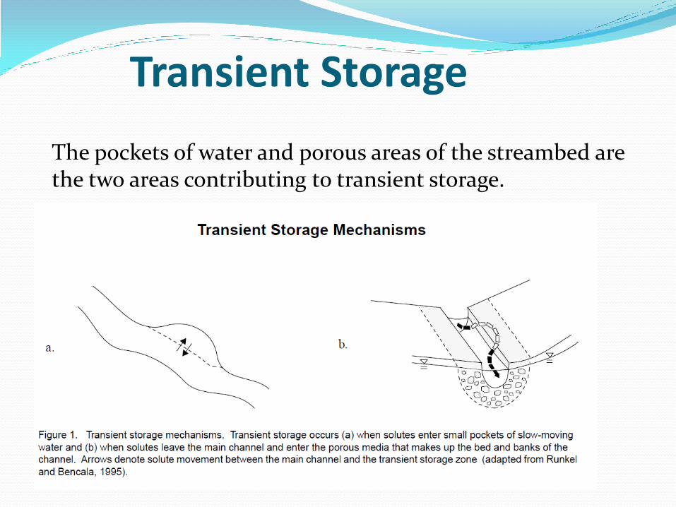
The pockets of water and porous areas of the streambed are the two areas contributing to transient storage.

Transient Storage

Why OTIS? Estimating nutrient uptake in streams – Denis Newbold

Studying particle dynamics – transport ,deposition and suspension – Denis Newbold

Estimating the exchange of water between stream and sediments

Assessing the fate of contaminants that are released into surface waters

Governing Differential Equations in OTIS

Assumptions

The primary Assumption * Solute concentration varies only in the longitudinal direction. Model assumptions * The physical processes that affect solute concentrations include advection, dispersion, lateral inflow, lateral outflow, and transient storage. * Advection, dispersion, lateral inflow, and lateral outflow do not occur in the storage zone.

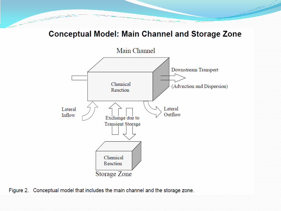
Governing Differential Equations – the Conservative Case In the Main Channel:

𝝏𝐶

𝝏𝑡= −

𝑄

𝐴 𝝏𝐶

𝝏𝑥+

1

𝐴

𝝏

𝝏𝑥𝐴𝐷

𝝏𝐶

𝝏𝑥+

𝑞𝐿𝐼𝑁

𝐴𝐶𝐿 − 𝐶 + 𝝰(𝐶𝑠 − 𝐶) (1)

In the storage-zone:

𝑑𝐶𝑠

𝑑𝑡= 𝝰

𝐴

𝐴𝑠(𝐶 − 𝐶𝑠) (2)

Where 𝐴 - main channel cross-sectional area [𝐿2] 𝐴𝑠 - storage zone cross-sectional area [𝐿2] 𝐶 – main channel solute concentration [M/𝐿3] 𝐶𝐿 - lateral inflow solute concentration [M/𝐿3] 𝐶𝑠 - storage zone solute concentration [M/𝐿3] 𝐷 – dispersion coefficient [𝐿2/T] 𝑄 – volumetric flow rate [𝐿3/T] 𝑞𝐿𝐼𝑁 - lateral inflow rate[𝐿3/T-L] 𝑡 – time [T] 𝑥 – distance [L] 𝝰 – storage zone exchange coefficient [/T]

A reach is defined as a continuous distance along which model parameters remain constant.

a single reach

several reaches

Each reach is subdivided into a number of computational elements or segments.

Segmentation Scheme

Boundary Conditions

Upstream condition: the concentration at the upstream boundary (𝐶𝑏𝑐) is fixed.

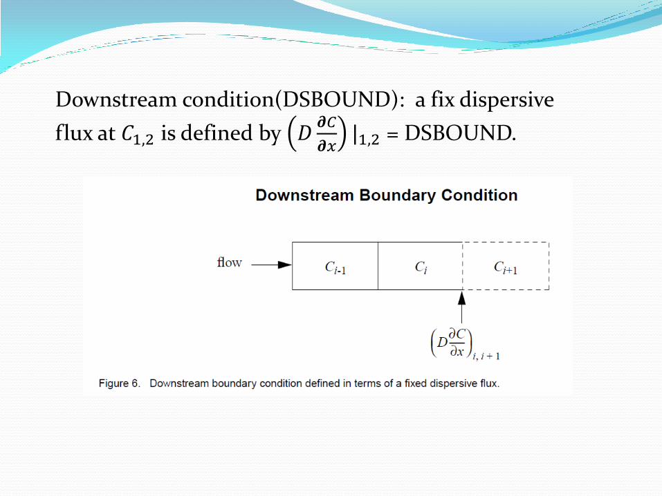
Downstream condition(DSBOUND): a fix dispersive

flux at 𝐶1,2 is defined by 𝐷𝝏𝐶

𝝏𝑥|1,2 = DSBOUND.

Numerical Solutions

After applying the finite-difference approximations, Eqn(1) becomes:

𝑑𝐶

𝑑𝑡= 𝐿(𝐶) +

𝑞𝐿𝐼𝑁

𝐴𝑖𝐶𝐿 − 𝐶𝑖 + 𝝰(𝐶𝑠 − 𝐶𝑖) (3)

Where

𝐿 𝐶 = −𝑄

𝐴𝑖

𝐶𝑖+1 − 𝐶𝑖−1

2Δ𝑥+

1

𝐴𝑖

𝐴𝐷 𝑖,𝑖+1 𝐶𝑖+1 − 𝐶𝑖 − 𝐴𝐷 𝑖−1,𝑖(𝐶𝑖 − 𝐶𝑖−1)

2Δ𝑥2

Here, i subscripts the segments, and Δ𝑥 is the length of each segment.

Crank-Nicolson Method

The time derivate dC/dt, is estimated using a forward difference approximation:

(4)

Δt – the integration time step [T]

j – denotes the value of a parameter or variable at the current time

j+1 – denotes the value of a parameter or variable at the advanced time

Eqn(3) and (4) were developed into (5) for all the segments in the modeled system,

(5)

A hypothetical set of equations representing a five-segment system

Systems of equations above can be efficiently solved using the Thomas Algorithm.

Applications of OTIS

OTIS/OTIS-P Flow Chart

InjMetaData.DAT

WTW or SYI********_date.txt

flow_NNN.inp params_NNN.inp

OTIS_Wrapper.sas

InjMetaData_bldr.sas

InjMetadataMerge_c.sas

BkgdCorrection_c.sas

ModelAreaFlow_c.sas

Injmetadata.sas7bdat

InjMetaDataMerge.sas7bdat

bkgdc.sas7bdat

ModelAreaFlow.sas7bdat

Run runsalt in DOS

WTW or YSI********.sas7bdat

Salt_bldr.sas

Salt_bldr_rename.sas

Run buildcond in DOS

OTIS.exe

OTIS-P.exe

Otisp_indata_NNN.inp Control.inp

Results_NNN.out Echo_NNN.out

Params_NNN.out

OTISSumm.txt

Graphs and parameters in SAS

star.inp

OTIS_Wrapper.sas

ModelRunLog***.xlsx

Manually input

Manually input

CF.sas7bdat

Conversionfactor_c.sas

spiral20yy_data_dionex.sas7bdat Spiral17_labelchem_merge.sas

swrc.label_yyyy

dx17_all_recalib_c.sas7bdat

Spiral17_labelchem.xlsx

Manually input

ModelAreaFlow_br.sas7bdat

Manually input

ModelAreaFlow_br_c.sas

Our OTIS/OTIS-P model

Flumes Stream

Solute (conservative) Yes Yes

Spatially uniform Yes No (assumed uniformity)

Temporally steady flow Yes No (assumed steady flow during experiment)

lateral inflow No Yes (assumed no inflow)

Lateral outflow No No

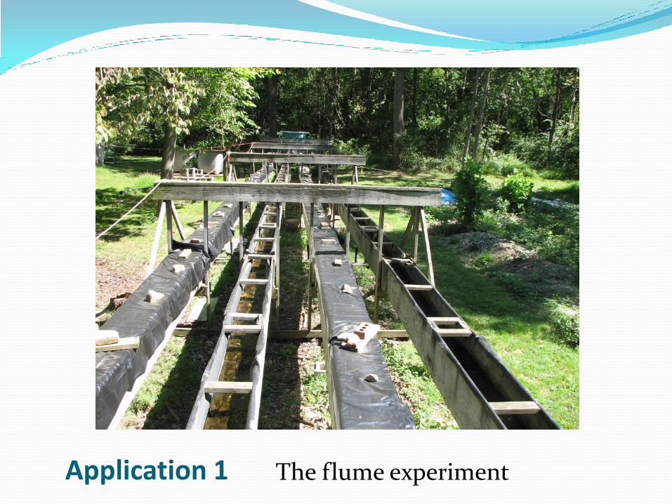
Application 1 The flume experiment

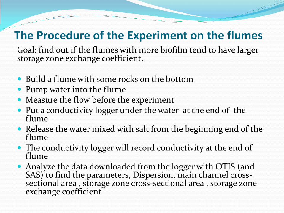
The Procedure of the Experiment on the flumes Goal: find out if the flumes with more biofilm tend to have larger storage zone exchange coefficient. Build a flume with some rocks on the bottom Pump water into the flume Measure the flow before the experiment Put a conductivity logger under the water at the end of the

flume Release the water mixed with salt from the beginning end of the

flume The conductivity logger will record conductivity at the end of

flume Analyze the data downloaded from the logger with OTIS (and

SAS) to find the parameters, Dispersion, main channel cross-sectional area , storage zone cross-sectional area , storage zone exchange coefficient

OTIS graphical result for one of the flume experiments

Increase Decrease

Disp Lower max and wider

A Shift right and slightly wider

As Lower max and extend tail

Alpha Lower max and steepen tail

Results after Changing Parameters

Left Graph -OTIS Right Graph-OTIS-P

Dispersion 3.0000E-02 1.99078E-02

Area 1.21700E-02 1.33145E-02

Area2 1.08165E-03 1.10478E-03

Alpha 8.24720E-03 5.07259E-03

OTIS-P does not work when the input parameters are too different from the true values.

An Example of failed modeling in OTIS-P

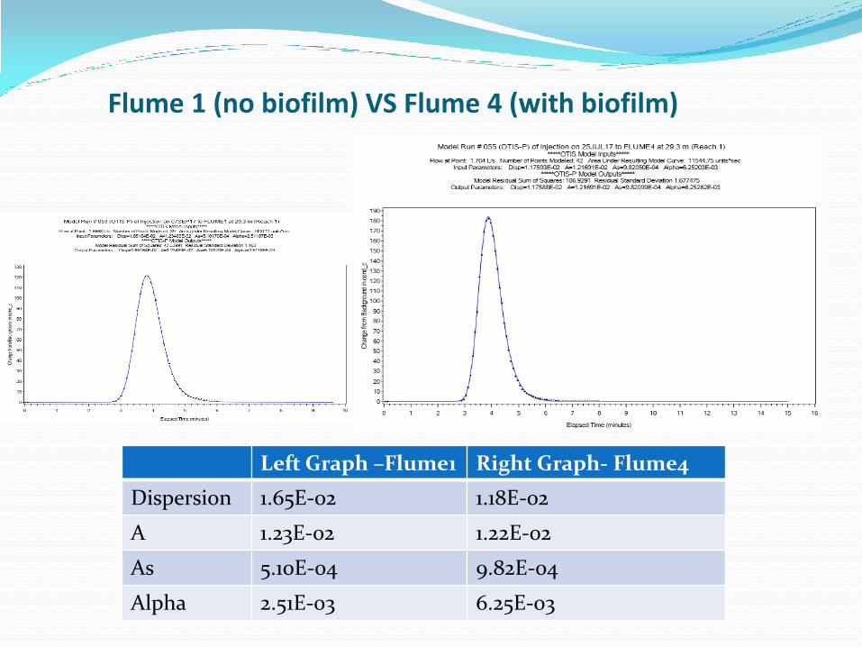
Flume 1 (no biofilm) VS Flume 4 (with biofilm)

Left Graph –Flume1 Right Graph- Flume4

Dispersion 1.65E-02 1.18E-02

A 1.23E-02 1.22E-02

As 5.10E-04 9.82E-04

Alpha 2.51E-03 6.25E-03

Conclusion

The biofilm made the storage zone exchange coefficient and storage zone cross-sectional area larger.

Application 2 - experiments on the Stream

Purpose: we want to find out how trees and branches that fell into the stream affect transient storage in White Clay Creek

In Sep. and Oct. 2017, we

• Selected a reach about 200 meters long and marked five stations within the reach;

• Set up the conductivity loggers at the injection site located upstream from the injection site (for background), and at stations 1 and 5.

• Set up barrels and equipment at the injection site and metered NaCl and NaBr to the stream using a pump;

• The pump worked for 17 hours and the loggers recorded for more than 24 hours.

• The data in the loggers were downloaded to computer and analyzed for the four parameters, Disp, Area, Area 2 and Alpha with OTIS/OTIS-P.

Then we will place woody debris into the stream on the site(s)in White Clay Creek.

Next year, run the experiment again to see the change of the four parameters.

NaCl and NaBr are metered into the stream

Conductivity Meter

OTIS/OTIS-P Results for Meadow Reach

OTIS OTIS-P

Flux input in param file; flux is considered to be uniform.

Flux input in param file; flux is different for each barrel.

Best OTIS-P Result for Meadow Reach

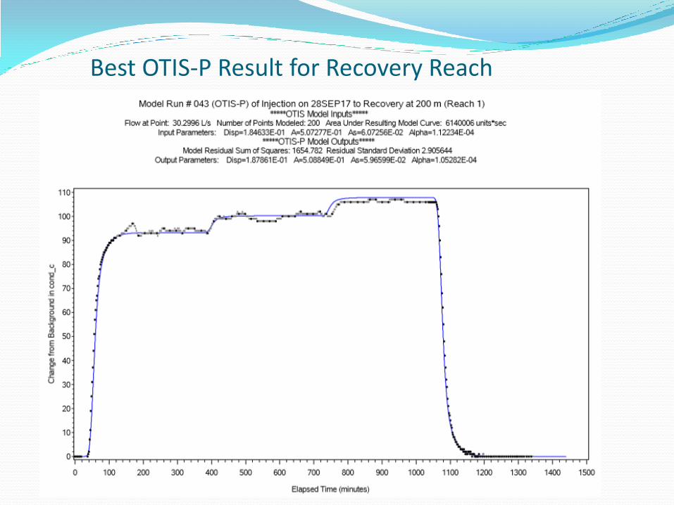
Best OTIS-P Result for Recovery Reach

Best OTIS-P Result for Forested Reach

Summary

Meadow Recovery Forested

Dispersion (m2/s)

Main Channel Cross- sectional Area (m2)

Storage Zone Cross-sectional Area (m2)

Storage Zone Exchange Coefficient Alpha (s-1)

0.122

0.479

0.0697

1.16E-04

0.899

0.464

0.0570

5.05E-05

0.188

0.509

0.0597

1.05E-04

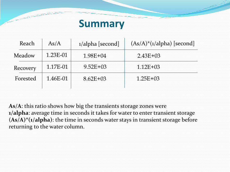
Summary

Reach

Meadow

Recovery

Forested

As/A 1/alpha [second] (As/A)*(1/alpha) [second]

1.23E-01 1.98E+04 2.43E+03

1.17E-01 9.52E+03 1.12E+03

1.46E-01 8.62E+03 1.25E+03

As/A: this ratio shows how big the transients storage zones were 1/alpha: average time in seconds it takes for water to enter transient storage (As/A)*(1/alpha): the time in seconds water stays in transient storage before returning to the water column.

The size of the transient storage zone was similar among reaches.

The transient storage exchange coefficient in the forested reach was higher than the other two reaches.

Conclusion

Any Questions?

Citations

Robert Runkel, USGS, www.usgs.gov/staffprofiles/robert-runkel?qtstaff_profile_science_products=3#qt-staff_profile_science_products.

Runkel, Rob. “OTIS.” USGS Water Resources, USGS, water.usgs.gov/software/OTIS/.