Résumé of the AIAA FDTC Low Reynolds Number Discussion Group’s Canonical Cases

Michael V. OL*

U.S. Air Force Research Laboratory

Aaron Altman† University of Dayton

Jeff D. Eldredge‡

University of California, Los Angeles

Daniel J. Garmann§ University of Cincinnati and U.S. Air Force Research Laboratory

Yongsheng Lian**

University of Louisville

The AIAA Fluid Dynamics Technical Committee’s Low Reynolds Number Discussion Group has introduced several “canonical” pitch motions, with objectives of (1) experimental-numerical comparison, (2) assessment of closed-form models for aerodynamic force coefficient time history, and (3) exploration of the vast and rather amorphous parameter space of the possible kinematics. The baseline geometry is a flat plate of nominally 2.5% thickness and round edges, wall-to-wall in ground test facilities and spanwise-periodic or 2D in computations. Motions are various smoothings of a linear pitch ramp, hold and return, of 40o and 45o amplitude. In an attempt to discern acceleration effects, sinusoidal and linear-ramp motions are compared, where the latter have short runs of high acceleration and thus high noncirculatory lift and pitch. Parameter variations include comparison of the flat plate with an airfoil and ellipse, variation of reduced frequency, pitch pivot point location and comparison of pitch to quasi-steady equivalent plunge. All motions involve strong leading edge vortices, whose growth history depends on pitch pivot point location and reduced frequency, and which can persist over the model suction-side for well after motion completion. Noncirculatory loads were indeed found to be localized to phases of motion where acceleration was large. To the extent discernable so far, closed-form models of lift coefficient on the pitch upstroke are relatively straightforward, but not so on the downstroke, where motion history effects complicate the return from stall. Broad Reynolds number independency, in flowfield evolution and lift coefficient, was found in the 103 to 104 range.

Nomenclature U∞ Free-stream velocity, cm/s c Airfoil/plate/wing chord, cm x/c Airfoil/plate/wing chord fraction, or pitch pivot location h Dimensionless plunge amplitude Re Reynolds Number, Re= U∞ c/ν. t* Convective time, t* = c/U∞. θ& Pitch rate, radians per second. A Pitch amplitude, deg. K Reduced pitch rate, ∞= UcK 2θ&

* Aerospace Engineer, Air Vehicles Directorate, AFRL/RBAA, Bldg. 45, 2130 8th St., Wright-Patterson AFB, OH 45433-7542; AIAA Associate Fellow, Michael.Ol@wpafb.af.mil † Associate Professor, Department of Mechanical and Aerospace Engineering, 300 College Park Dr., Dayton, OH 45469-0238: AIAA Associate Fellow ‡ Associate Professor, Mechanical & Aerospace Engineering, University of California, Los Angeles, Los Angeles, CA, 90095-1597, AIAA Member § Aerospace Engineering Graduate Student, AIAA Member **Assistant Professor, Department of Mechanical Engineering, AIAA Senior Member

48th AIAA Aerospace Sciences Meeting Including the New Horizons Forum and Aerospace Exposition4 - 7 January 2010, Orlando, Florida

AIAA 2010-1085

Copyright © 2010 by the American Institute of Aeronautics and Astronautics, Inc.The U.S. Government has a royalty-free license to exercise all rights under the copyright claimed herein for Governmental purposes.All other rights are reserved by the copyright owner.

Introduction Micro Air Vehicles (MAVs) have been a sturdy source of motivation for fascinating problems in

fundamental aerodynamics, and can be considered as prototypical for capturing many questions at the interface between fundamental classical aerodynamics and applied problems of airplane performance. Large flow unsteadiness, massive separation, motion-history effects, laminar to turbulent transition, three-dimensional flowfields dominated by vortex and acceleration effects are of substantial relevance to the MAV flight problem, regardless of vehicle configuration. Progress has been substantial, but is largely episodic and understandably rife with the biases of each individual researcher, such that it is difficult to discern whether a given problem has been reduced to parameter dependency or whether it remains conceptually unclear. Contingent upon our own biases, we can illustrate several subjects with a sobering dearth of basic understanding – or at least, of basic consensus:

• There exist no validated rapid, robust computational aerodynamic models for conceptual design/sizing or real-time flight control across the anticipated range of flight regimes for flapping wing or maneuvering MAVs. Examples of flight regimes include gust-perturbed cruise, maneuvering flight, launch and perching. One would like a tool at the level of XFOIL1 for massively unsteady problems at the MAV Reynolds number range.

• It remains unclear to what extent traditional analytical models, based on potential flow, superposition and so forth – can be applicable to first order for flow problems involving large separation and unsteadiness, and nonplanar wakes.

• Doubts linger on the utility of laboratory-type abstractions of flight articles, in particular in the passage from 2D problems to 3D planforms and what happens to the various 2D-specific observations about vortex dynamics when applied to 3D planforms.

• How crucial is it to “correctly” resolve the time-dependent flowfield if the objective is to simply calculate lift coefficient and pitching moment time history?

The AIAA Fluid Dynamics Technical Committee (FDTC) Low Reynolds Number Discussion Group (LRDG) selected a set of ramp-hold-return cases as representative of problems in unsteady aerodynamics, initially in two dimensions. The motivation was to avoid periodic motion conditions, where barring long-time relaxation of start-up transients, the response should be periodic as well. Experiments should be tractable for both wind tunnels and water tunnels, which places bounds on Reynolds number and reduced frequency. The angle of attack range should be into deep stall, and the angle of attack history relevant to applications such as perching, maneuvering, gust loading and flapping. On the numerical side, the Re range should bracket laminar and transitional cases, and be amenable to approaches ranging from immersed boundary methods to 3D LES. Another concern was the role of the so-called noncirculatory or apparent-mass forces2. Whenever the wing is accelerating, it is accelerating a volume of fluid around it. The pressure gradient necessary for that acceleration, when integrated around the wing surface, produces a net lift and pitching moment, which for periodic sinusoidal motions (the simplest case) is proportional to the frequency of oscillation squared. The question of what proportion of total lift is from vortical effects – bound and shed vorticity – vs. noncirculatory effects – is perhaps moot for computation of forces from solving the Navier-Stokes equations, or when measuring force directly with a balance. But it is important in searching for closed-form analytic or quasi-analytic models, because noncirculatory forces are at least in principle reducible from potential flow, and therefore amenable to straightforward derivation even for complicated motions and geometries. There is however a controversy as to the relevance of noncirculatory loads for practical applications such as flapping. The series of results by Dickson, Dickinson et al.3,4 suggests that noncirculatory loads are limited to small time intervals in the motion history, while results for high-frequency periodic sinusoidal oscillations (such as Visbal5) imply precisely the contrary. This is of course a gross oversimplification, as the various conditions differ in hover vs. presence of free-stream, role of 3D effects, Reynolds number and so forth. But this only adds to the controversy.

A first iteration of results on ramp-hold-return motions was presented at a special-session at the 39th AIAA Fluid Dynamics Conference, June 2009. We summarize these results below. Experience from the parallel experiments and computations comprising the first iteration of results led to a redefinition of the so-called canonical motions, which are described here in detail, and for which preliminary results are also given.

Definition of Motion Parameters We first discuss the suggested motions for common study, in the hope that this would be of general interest for future work and a departure point for parameter studies. We then recapitulate the history of the motion definitions and mention some earlier versions.

A. The Suggested Canonical Kinematics

We define a family of motions with shared angle of attack range and peak angle of attack rate, but in one case with nominally sinusoidal (nearly one-minus-cosine function) angle of attack history, and in another of trapezoidal history, where accelerations are limited to narrow regions of time, and are zero otherwise. The unsmoothed trapezoidal motion has an upgoing and downgoing linear ramp in angle of attack, defined nondimensionally as 20.02 ==

∞UcK θ& , with pivot about the leading edge.

To avoid model vibration in experiments and numerical instabilities in the computations, and delta-function spikes in calculated noncirculatory force, all motions are smoothed. For a ramp in going from 0 degrees angle of attack to 45 degrees, the first 10% (4.5 degrees) can be replaced with a sinusoid tangent to the baseline ramp, and similarly in approaching the “hold” portion at the peak angle of attack, and again on the downstroke. The result is a piecewise sinusoidal and piecewise linear fit. This unfortunately has discontinuities in the angle of attack second derivative, and was therefore replaced by an alternative C∞ smoothing function developed by Eldredge12. The smoothing function G(t) is defined as:

−−−−

=∞∞

∞∞

)/)(cosh()/)(cosh()/)(cosh()/)(cosh(

ln)(32

41

cttaUcttaUcttaUcttaU

tG

where a is a free parameter, c is the chord, and the times t1 through t4 are: t1 = time from reference 0 until when the sharp corner of the unsmoothed ramp would start t2 = t1 + duration of the pitch upstroke, until the sharp corner where the hold would have begun t3 = t2 + the unsmoothed hold time at maximum alpha t4 = t3 + the unsmoothed pitch downstroke duration

Then, with the pitch amplitude A = 45 deg, the smoothed motion becomes

))(max()()(

tGtGAt =α

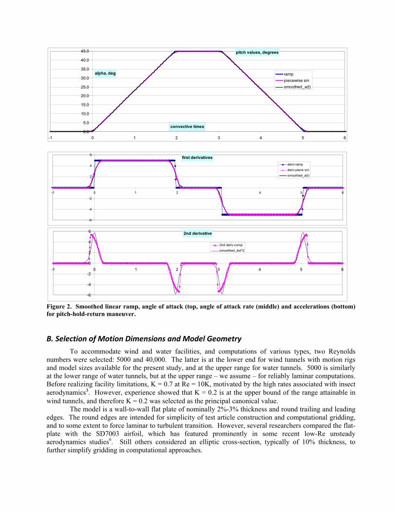
By varying the parameter a, G(t) becomes a parametrization of smoothing from true trapezoid all the way to approximate sinusoid. A large value of a leads to an abrupt acceleration, presumably with large spikes in noncirculatory lift and pitch (but not drag/thrust, which has no noncirculatory portion).

The relation between linear ramp and sinusoid, in Figure 1, is constrained by matching the amplitude and peak pitch rate between the two. So for a linear ramp with dimensional pitch rate θ& , the duration of the linear ramp relates to the frequency of the sinusoid as ftt π2

112 =− , and the length of the

linear ramp’s hold time becomes ff

ttπ1

21

23 −=− . Setting a = 2 produces a close fit between the sinusoid,

)2cos(1()( ftAt πθ −= ), while a = 11 is in turn a close approximation to the 10% sinusoidal smoothing of an otherwise linear ramp (Figure 2). Physically, the pitch ramp-hold-return motions in the K range of 0.2-0.7 and Re range of O(104) feature the growth of a large leading edge vortex (LEV) that does not pinch off until the pitching motion ends. The hold at maximum angle of attack lasts roughly as long as it would take the LEV to convect from leading to trailing edge at free-stream speed. The downstroke is proposed as a prototypical motion to study flow “memory” effects, where upon returning to zero angle of attack the flow is still recovering from massive separation. We speculated, at this point, that a quasi-steady model with the appropriate tuning can account for lift coefficient time history over the entire upstroke (other than for noncirculatory effects), but will fail on the downstroke. For applications such as insect flapping, there really is no downstroke in the sense of the present case, as the motion essentially starts afresh on every half-stroke. It is perhaps for this reason that quasi-steady models for insect-type flapping are successful.3 Thus, there are four main cases: two Reynolds numbers and two values of the smoothing parameter a, of 2 and 11.

pitch values, degrees

0.0

5.0

10.0

15.0

20.0

25.0

30.0

35.0

40.0

45.0

-1 0 1 2 3 4 5 6

convective times

alpha, deg ramppiecewise sinsmoothed_a(t)

first derivatives

-6

-4

-2

0

2

4

6

-1 0 1 2 3 4 5 6

deriv rampderiv piece sinsmoothed_a(t)

2nd derivative

-1.5

-1

-0.5

0

0.5

1

1.5

-2 -1 0 1 2 3 4 5 6 7

2nd deriv compsmoothed_dot 2̂

Figure 1. Sinusoidal ramp, angle of attack (top, angle of attack rate (middle) and accelerations (bottom) for pitch-hold-return maneuver.

pitch values, degrees

0.0

5.0

10.0

15.0

20.0

25.0

30.0

35.0

40.0

45.0

-1 0 1 2 3 4 5 6

convective times

alpha, deg ramppiecewise sinsmoothed_a(t)

first derivatives

-6

-4

-2

0

2

4

6

-1 0 1 2 3 4 5 6

deriv rampderiv piece sinsmoothed_a(t)

2nd derivative

-6

-4

-2

0

2

4

6

-1 0 1 2 3 4 5 6

2nd deriv compsmoothed_dot 2̂

Figure 2. Smoothed linear ramp, angle of attack (top, angle of attack rate (middle) and accelerations (bottom) for pitch-hold-return maneuver.

B. Selection of Motion Dimensions and Model Geometry

To accommodate wind and water facilities, and computations of various types, two Reynolds numbers were selected: 5000 and 40,000. The latter is at the lower end for wind tunnels with motion rigs and model sizes available for the present study, and at the upper range for water tunnels. 5000 is similarly at the lower range of water tunnels, but at the upper range – we assume – for reliably laminar computations. Before realizing facility limitations, K = 0.7 at Re = 10K, motivated by the high rates associated with insect aerodynamics3. However, experience showed that K = 0.2 is at the upper bound of the range attainable in wind tunnels, and therefore K = 0.2 was selected as the principal canonical value. The model is a wall-to-wall flat plate of nominally 2%-3% thickness and round trailing and leading edges. The round edges are intended for simplicity of test article construction and computational gridding, and to some extent to force laminar to turbulent transition. However, several researchers compared the flat-plate with the SD7003 airfoil, which has featured prominently in some recent low-Re unsteady aerodynamics studies6. Still others considered an elliptic cross-section, typically of 10% thickness, to further simplify gridding in computational approaches.

C. Non‐Canonical Kinematics: Antecedents

Arrival at the motions described in Figure 1 and Figure 2 was somewhat tortuous and only possible after multiple iterations. Most of the work presented in the present review is of related but different motion kinematics and comparisons should be treated as suggestive but hardly dispositive.

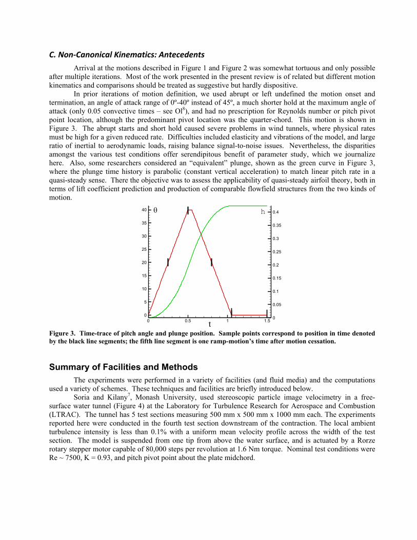
In prior iterations of motion definition, we used abrupt or left undefined the motion onset and termination, an angle of attack range of 0º-40º instead of 45º, a much shorter hold at the maximum angle of attack (only 0.05 convective times – see Ol8), and had no prescription for Reynolds number or pitch pivot point location, although the predominant pivot location was the quarter-chord. This motion is shown in Figure 3. The abrupt starts and short hold caused severe problems in wind tunnels, where physical rates must be high for a given reduced rate. Difficulties included elasticity and vibrations of the model, and large ratio of inertial to aerodynamic loads, raising balance signal-to-noise issues. Nevertheless, the disparities amongst the various test conditions offer serendipitous benefit of parameter study, which we journalize here. Also, some researchers considered an “equivalent” plunge, shown as the green curve in Figure 3, where the plunge time history is parabolic (constant vertical acceleration) to match linear pitch rate in a quasi-steady sense. There the objective was to assess the applicability of quasi-steady airfoil theory, both in terms of lift coefficient prediction and production of comparable flowfield structures from the two kinds of motion.

0 0.5 1 1.5t0

5

10

15

20

25

30

35

40

0

0.05

0.1

0.15

0.2

0.25

0.3

0.35

0.4θ h

Figure 3. Time-trace of pitch angle and plunge position. Sample points correspond to position in time denoted by the black line segments; the fifth line segment is one ramp-motion’s time after motion cessation.

Summary of Facilities and Methods The experiments were performed in a variety of facilities (and fluid media) and the computations

used a variety of schemes. These techniques and facilities are briefly introduced below. Soria and Kilany7, Monash University, used stereoscopic particle image velocimetry in a free-surface water tunnel (Figure 4) at the Laboratory for Turbulence Research for Aerospace and Combustion (LTRAC). The tunnel has 5 test sections measuring 500 mm x 500 mm x 1000 mm each. The experiments reported here were conducted in the fourth test section downstream of the contraction. The local ambient turbulence intensity is less than 0.1% with a uniform mean velocity profile across the width of the test section. The model is suspended from one tip from above the water surface, and is actuated by a Rorze rotary stepper motor capable of 80,000 steps per revolution at 1.6 Nm torque. Nominal test conditions were Re ~ 7500, K = 0.93, and pitch pivot point about the plate midchord.

Figure 4. Experimental setup at Monash University; water tunnel (left) and stereo PIV camera setup in tunnel test section (right).

Ol8, at the U.S. Air Force Research Laboratory Air Vehicles Directorate, also used a free-surface

water tunnel (Figure 5), relying primarily on conventional 2-component particle image velocimetry and dye injection. The “Horizontal Free-surface Water Tunnel” (HFWT) has a 46 cm wide by 61 cm high and 300 cm long test section and speed range of 3-45 cm/s. Turbulence intensity (based on u and v components) in the test section is estimated at 0.4% at U∞ = 30-40 cm/s. A surface skimmer plate mounted at the entrance to the test section and a sealed lid over the intake plenum (visible as plywood cover in Figure 5) damp sloshing in the tunnel. Above the test section is a three-degree-of-freedom oscillation rig, enabling pitch, plunge and streamwise fore-aft motion or “surge”, using three electric linear servo motors. Two motors mounted vertically above the test section actuate vertical “plunge rods”, which connect via bushings to the model at fixed points. The third motor tows the carriage holding the other two, together with the experiment, fore and aft. Depending on pivot point location, all three motors combine to produce pure-pitch. The model is mounted horizontally with the plunge rods at the model centerplane, in an intrusive but structurally stiff arrangement suitable for very aggressive motions.

Figure 5. Photographs of the AFRL water tunnel (left) flat-plate model installation in water tunnel (middle) and detail of dye injector tip (right).

Williams et al.9, at the Illinois Institute of Technology, conducted experiments on a semicircular planform and a nearly wall-to-wall plate in the Andrew Fejer Unsteady Flow Wind Tunnel (Figure 6). The test section has dimensions 610 mm x 610 mm in the cross section. The freestream speed is controlled by a variable speed (vector drive) 40 HP motor. The unique feature of the facility is a shutter system downstream of the test section, enabling a time-varying mean velocity profile, for example for gust-response testing. The mean flow speeds ranged from 2.8 m/s to 5.0 m/s. The freestream turbulence was measured to be 0.6 percent at U = 3 m/s over a bandwidth of 0.1 Hz to 30 Hz. The shutter system is capable of generating frequencies up to 3 Hz sinusoidal oscillation in the streamwise velocity component. The first

harmonic of the oscillation was more than 20 dB below the fundamental across the spectrum of frequencies used.

Figure 6. Andrew Fejer Unsteady Flow Wind Tunnel at IIT: semicircular model in test section (left) and

schematic of tunnel circuit (right).

Turning to the computations, Lian10, at the University of Louisville, used a pressure-Poisson

method to solve the incompressible Navier-Stokes equations. Both convection and diffusion terms are discretized using a second-order accurate central difference method. A second-order accurate split-step scheme with an Adam’s predictor corrector time-stepping method is adopted for the time integration. An overlapping moving grid approach is employed to dynamically update the grid due to the plate motion.

Garmann and Visbal11, at the University of Cincinnati and AFRL, respectively, used the compressible Navier-Stokes solver FDL3DI: a filtered, high-order, implicit large eddy simulation (ILES) scheme. 2D and 3D computations were compared. Eldredge et al.12 used a 2D viscous vortex particle method (VVPM). The method uses a fractional stepping procedure, in which the fluid convection, fluid diffusion, and vorticity creation are treated in separate substeps of each time increment. An advantage of this method over conventional fixed-grid schemes is that the computational elements are convecting particles that automatically adapt to the flow, which obviates the need for expensive mesh regeneration. Furthermore, the focus on vorticity provides natural computational efficiency and physical insight. Zheng et al.13 used an immersed boundary method to solve the incompressible Navier-Stokes equations in 2D, over a staggered nested Cartesian grid.

Results In Part A, we review the results presented at the 39th AIAA Fluid Dynamics Conference, June 2009. These are predominantly for the short-hold, 0-40º abrupt ramp. In Part B we present preliminary results for the canonical motions.

A. Short‐hold, Abrupt Ramp 0‐40 Motions

We first consider the baseline case of K = 0.7 and Re = 10,000, in linear pitch ramp from 0 to 40 degrees, a hold of only 0.05 convective times and ad hoc conditions for smoothing. Figure 7 shows contours of out-of-plane vorticity from PIV (Ol8, Re = 10000) and CFD (Lian10, Re = 10000 and Eldredge et al.12, Re = 1000). The original color schemes are retained, and in most cases the normalized contour levels are -36 to +36, in 13 levels, with the two levels bracketing -6 to +6 removed for clarity. Snapshots are taken as marked in Figure 3, at four instances: halfway on the upstroke (α=20º), right at the start of the hold, halfway along the downstroke, and right at completion of motion (α~0º).

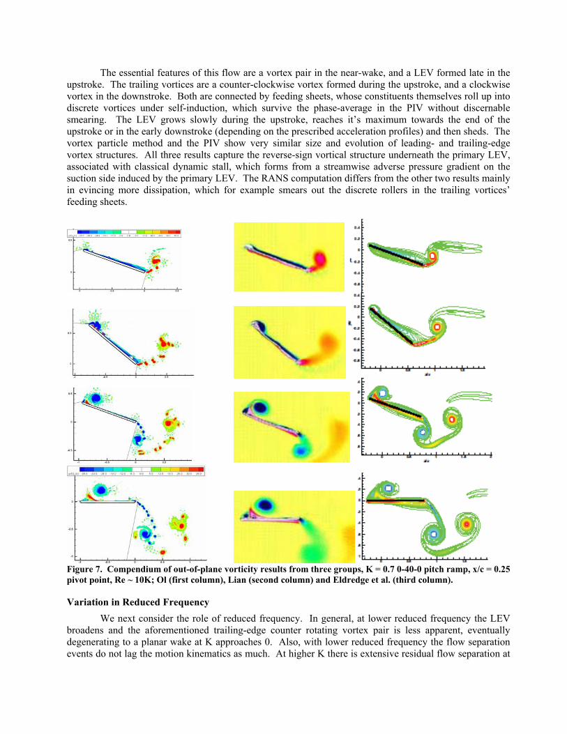
The essential features of this flow are a vortex pair in the near-wake, and a LEV formed late in the upstroke. The trailing vortices are a counter-clockwise vortex formed during the upstroke, and a clockwise vortex in the downstroke. Both are connected by feeding sheets, whose constituents themselves roll up into discrete vortices under self-induction, which survive the phase-average in the PIV without discernable smearing. The LEV grows slowly during the upstroke, reaches it’s maximum towards the end of the upstroke or in the early downstroke (depending on the prescribed acceleration profiles) and then sheds. The vortex particle method and the PIV show very similar size and evolution of leading- and trailing-edge vortex structures. All three results capture the reverse-sign vortical structure underneath the primary LEV, associated with classical dynamic stall, which forms from a streamwise adverse pressure gradient on the suction side induced by the primary LEV. The RANS computation differs from the other two results mainly in evincing more dissipation, which for example smears out the discrete rollers in the trailing vortices’ feeding sheets.

Figure 7. Compendium of out-of-plane vorticity results from three groups, K = 0.7 0-40-0 pitch ramp, x/c = 0.25 pivot point, Re ~ 10K; Ol (first column), Lian (second column) and Eldredge et al. (third column).

Variation in Reduced Frequency We next consider the role of reduced frequency. In general, at lower reduced frequency the LEV broadens and the aforementioned trailing-edge counter rotating vortex pair is less apparent, eventually degenerating to a planar wake at K approaches 0. Also, with lower reduced frequency the flow separation events do not lag the motion kinematics as much. At higher K there is extensive residual flow separation at

motion cessation, as seen in the bottom row of Figure 7. At low K the shed vortex system – if there even is one – is convecting past the airfoil trailing edge, and return to reattachment follows closely after motion cessation. This is of course intuitive, given the idea of quasi-steady response and its validity as a function of reduced frequency. These trends can be seen in the K=0.2 version of the aforementioned case, shown in Figure 8. Results include Eldredge et al.12, Re = 1000; Ol8, Lian10, and Garmann and Visbal11, all at Re = 10000; and Williams et al.9, for a motion with a longer hold and Re ~ 70K.

Figure 8. Compendium of out-of-plane vorticity contours from five groups, K = 0.2, 0-40-0 pitch ramp, Re ~ 10K, x/c = 0.25 pivot; Eldredge et al. (first column), Garmann and Visbal (second column) Ol (third column). Lian (fourth column) and Williams et al. (fifth column).

As seen in the computations of Garmann and Visbal11, and PIV results of Ol8 and Soria and Kilany7 (Figure 10 below), shed vortical structures have discrete fine-features that survive ensemble or phase averaging, especially in the near-wake. These discrete structures are likely from roll-up of shear layers due to self-induction. Computations of Eldredge et al12 at Re = 1000 show rough outlines of such structures, and preliminary results at Re = 10000 show their greater prominence. There is therefore evidence that this behavior is a function of Reynolds number, and to some extent discrete structures’ resolution is dependent on dissipation/resolution of the computational scheme, or the resolution of the PIV. The PIV of Williams et al.9, for example, is missing these features and generally has lower vorticity contour levels, evidently on account of the PIV grid used to calculate vorticity. The result of Garmann and Visbal11, here in 2D, shows the importance of full 3D treatment of LES. In a 2D LES approach the LEV formation and flowfield details on the upstroke are predicted in close accord with experimental observation, but on the downstroke the 2D computation overpredicts breakup of the coherent LEV into discrete vortices.

Effect of Pitch Pivot Point Figure 9 repeats the parameter study of Ol8, using dye injection from the leading edge. In going towards further-aft pitch pivot point, the LEV on the plate suction-side at peak angle of incidence becomes

more concentrated, and upon return to zero alpha, the LEV lifts further off of the plate surface. On the plate pressure side, a companion LEV becomes larger with increasing K on the upstroke. It is subsumed by the suction-side LEV on the downstroke. The pressure-side LEV is consistent with the interpretation of aft pivot point location as locally being a plunge of the plate at the leading edge; that is, the early pitch-up is locally a plunge-up at the leading edge, whence the flow separation should be on the bottom side of the plate. The trailing edge counter rotating vortex pair is strongest when pivoting at the leading edge, again consistent with the interpretation of a pitching motion as a local plunge, when the pivot point is far away.

Figure 9. Flat-plate 0º-40º-0º pitch, K = 0.70, Re = 10K; parameter study of pitch pivot point. x/c = 0.0 (top row), 0.25, 0.50, 0.75 and 1.0 (bottom row). Snapshots are going across the page, following marks as given in Figure 3.

Conceptually similar is the computational pitch pivot point parameter study by Lian10, given together with the x/c=0.5 pivot point PIV results of Soria and Kilany7 in Figure 10. For leading-edge pivot point location, the trailing vortex pair is strong enough for the RANS computation to resolve it decisively.

x/c = 0.0

x/c = 0.25

x/c = 0.50

x/c = 0.75

x/c = 1.0

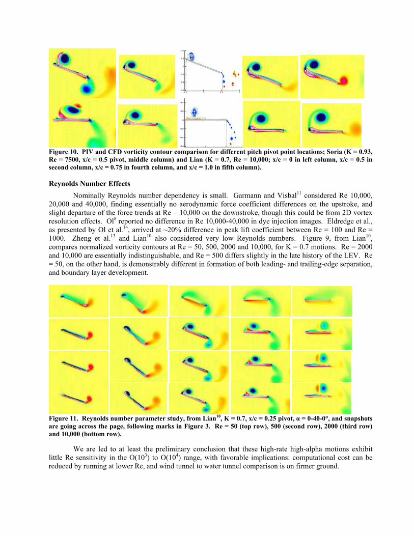
Figure 10. PIV and CFD vorticity contour comparison for different pitch pivot point locations; Soria (K = 0.93, Re = 7500, x/c = 0.5 pivot, middle column) and Lian (K = 0.7, Re = 10,000; x/c = 0 in left column, x/c = 0.5 in second column, x/c = 0.75 in fourth column, and x/c = 1.0 in fifth column).

Reynolds Number Effects Nominally Reynolds number dependency is small. Garmann and Visbal11 considered Re 10,000, 20,000 and 40,000, finding essentially no aerodynamic force coefficient differences on the upstroke, and slight departure of the force trends at Re = 10,000 on the downstroke, though this could be from 2D vortex resolution effects. Ol8 reported no difference in Re 10,000-40,000 in dye injection images. Eldredge et al., as presented by Ol et al.14, arrived at ~20% difference in peak lift coefficient between Re = 100 and Re = 1000. Zheng et al.13 and Lian10 also considered very low Reynolds numbers. Figure 9, from Lian10, compares normalized vorticity contours at Re = 50, 500, 2000 and 10,000, for K = 0.7 motions. Re = 2000 and 10,000 are essentially indistinguishable, and Re = 500 differs slightly in the late history of the LEV. Re = 50, on the other hand, is demonstrably different in formation of both leading- and trailing-edge separation, and boundary layer development.

Figure 11. Reynolds number parameter study, from Lian10, K = 0.7, x/c = 0.25 pivot, α = 0-40-0°, and snapshots are going across the page, following marks in Figure 3. Re = 50 (top row), 500 (second row), 2000 (third row) and 10,000 (bottom row).

We are led to at least the preliminary conclusion that these high-rate high-alpha motions exhibit little Re sensitivity in the O(103) to O(104) range, with favorable implications: computational cost can be reduced by running at lower Re, and wind tunnel to water tunnel comparison is on firmer ground.

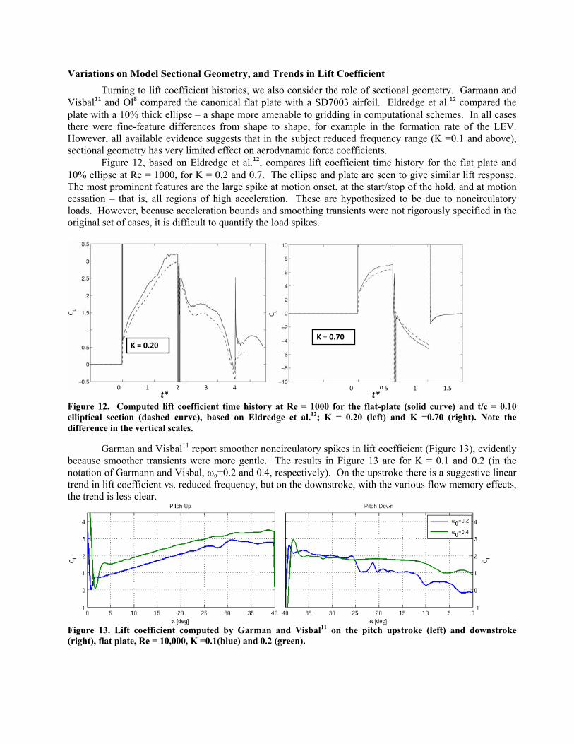
Variations on Model Sectional Geometry, and Trends in Lift Coefficient Turning to lift coefficient histories, we also consider the role of sectional geometry. Garmann and Visbal11 and Ol8 compared the canonical flat plate with a SD7003 airfoil. Eldredge et al.12 compared the plate with a 10% thick ellipse – a shape more amenable to gridding in computational schemes. In all cases there were fine-feature differences from shape to shape, for example in the formation rate of the LEV. However, all available evidence suggests that in the subject reduced frequency range (K =0.1 and above), sectional geometry has very limited effect on aerodynamic force coefficients. Figure 12, based on Eldredge et al.12, compares lift coefficient time history for the flat plate and 10% ellipse at Re = 1000, for K = 0.2 and 0.7. The ellipse and plate are seen to give similar lift response. The most prominent features are the large spike at motion onset, at the start/stop of the hold, and at motion cessation – that is, all regions of high acceleration. These are hypothesized to be due to noncirculatory loads. However, because acceleration bounds and smoothing transients were not rigorously specified in the original set of cases, it is difficult to quantify the load spikes.

Figure 12. Computed lift coefficient time history at Re = 1000 for the flat-plate (solid curve) and t/c = 0.10 elliptical section (dashed curve), based on Eldredge et al.12; K = 0.20 (left) and K =0.70 (right). Note the difference in the vertical scales.

Garman and Visbal11 report smoother noncirculatory spikes in lift coefficient (Figure 13), evidently because smoother transients were more gentle. The results in Figure 13 are for K = 0.1 and 0.2 (in the notation of Garmann and Visbal, ωo=0.2 and 0.4, respectively). On the upstroke there is a suggestive linear trend in lift coefficient vs. reduced frequency, but on the downstroke, with the various flow memory effects, the trend is less clear.

Figure 13. Lift coefficient computed by Garman and Visbal11 on the pitch upstroke (left) and downstroke (right), flat plate, Re = 10,000, K =0.1(blue) and 0.2 (green).

K = 0.20 K = 0.70

0 0.5 1 1.5 t*

0 1 2 3 4 t*

Similar trends were found by Eldredge et al.12,14; Figure 14 reports lift coefficient for a range of reduced frequencies on the upstroke and downstroke, for Re = 100 and 1000, for a 10%-thick elliptical section. Again, Re effects are benign. But the main observation is that if lift is normalized by reduced frequencies, then on the upstroke all lift curves collapse to essentially one curve. To substantiate this further, we need agreement on the motion smoothing transients, and to better compare with experiment – especially in wind tunnels – we need a longer hold at the pitch angle extremum. We pursue this in section B of the results.

Figure 14. Computed lift coefficient time history for 10%-thick elliptical section for the pitch upstroke, Re = 100 (top row) and Re = 1000 (bottom row); direct results (left column) and rescaled by reduced frequency (right column)14.

Pitch vs. Plunge We close the survey of results on the pitch-ramp canonical problem from the 39th AIAA Fluid Dynamics Conference, June 2009, by considering pitch vs. plunge. Putative equivalence between pitch and plunge was motivated in Figure 3, and dye injection results are given in Figure 15, based on Ol8, for both the flat-plate and the SD7003 airfoil. In short, the LEV evolution between pitch and plunge is qualitatively very similar, but the near-wake and trailing vortices are very different indeed. Unfortunately, no force measurements or computations are available.

Re = 1000Re = 1000

Re = 100 Re = 100

K = 1.05

K = 0.35

K = 0.53

K = 0.70

K = 0.88

K = 1.05

K = 0.35

K = 0.53

K = 0.70

K = 0.88

θ (deg)

θ (deg) θ (deg)

θ (deg)

Figure 15. Dye injection results of Ol8 for “equivalent” plunge: flat plate (top row) and SD7003 airfoil (bottom row); compare to second row of Figure 9 above.

B. The Canonical Cases

We now return to the motions plotted in Figure 1 and Figure 2. Dye injection results from the AFRL water tunnel for Re = 5000 are given in Figure 16. Again there is a parameter study of pitch pivot point location. On the upstroke, growth of the LEV is faster, the closer the pivot point is to the leading edge. The starting vortex from pitch-ramp onset is also weaker. Thus, on the upstroke at least until around α~30º, one can state that the closer to pivot point to the leading edge, the more benign the flow separation overall. But in the subsequent motion history, the role of pivot point diminishes, such that by halfway on the downstroke, LE-pivot and TE-pivot are hard to distinguish. Sinusoidal vs. ramp motions, both pivoting at the LE, show very little difference on the upstroke, through the hold. The main difference is that the sinusoidal motion, being less abrupt, has a smaller TE starting vortex. Late into the downstoke some differences appear in what remains of the LEV; namely, for the sinusoid there is a longer route towards flow reattachment after returning to zero angle of attack. But overall the sinusoidal and ramp flowfields are similar.

LE pivot 0.25c pivot TE pivot LE sinusoid

α=22.5º

α=33.75º

α=11.25º

α=45º

α=33.75º

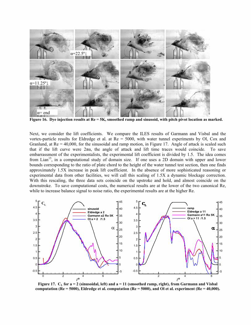
Figure 16. Dye injection results at Re = 5K, smoothed ramp and sinusoid, with pitch pivot location as marked.

Next, we consider the lift coefficients. We compare the ILES results of Garmann and Visbal and the vortex-particle results for Eldredge et al. at Re = 5000, with water tunnel experiments by Ol, Cox and Granlund, at Re = 40,000, for the sinusoidal and ramp motion, in Figure 17. Angle of attack is scaled such that if the lift curve were 2πα, the angle of attack and lift time traces would coincide. To save embarrassment of the experimentalists, the experimental lift coefficient is divided by 1.5. The idea comes from Lian15, in a computational study of domain size. If one uses a 2D domain with upper and lower bounds corresponding to the ratio of plate chord to the height of the water tunnel test section, then one finds approximately 1.5X increase in peak lift coefficient. In the absence of more sophisticated reasoning or experimental data from other facilities, we will call this scaling of 1.5X a dynamic blockage correction. With this rescaling, the three data sets coincide on the upstroke and hold, and almost coincide on the downstroke. To save computational costs, the numerical results are at the lower of the two canonical Re, while to increase balance signal to noise ratio, the experimental results are at the higher Re.

0 2 4 6t*

-0.5

0

0.5

1

1.5

2

2.5

3

3.5

4

4.5

5

-5

0

5

10

15

20

25

30

35

40

45

sinusoidEldredge a 2Garmann a2 Re 5KOl a = 2 /1.5

α

CL

2 4 6

t*

-0.5

0

0.5

1

1.5

2

2.5

3

3.5

4

4.5

5

-5

0

5

10

15

20

25

30

35

40

45

rampEldredge a 11Garmann a11 Re 5KOl a = 11 /1.5

α

CL

α

CL

α

CL

α

CL

α

CL

α

CL

α

CL

α

CL

α

CL

α

CL

α

CL

α

CL

α

CL

α

CL

α

CL

α

CL

α

CL

α

CL

α

CL

α

CL

α

CL

α

CL

α

CL

α

CL

Figure 17. CL for a = 2 (sinusoidal, left) and a = 11 (smoothed ramp, right), from Garmann and Visbal

computation (Re = 5000), Eldredge et al. computation (Re = 5000), and Ol et al. experiment (Re = 40,000).

α=22.5º↓

α=11.25º↓

α= end

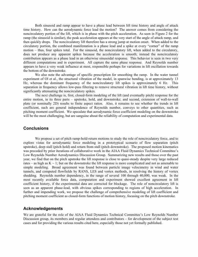
Both sinusoid and ramp appear to have a phase lead between lift time history and angle of attack time history. How can the aerodynamic force lead the motion? The answer comes from considering the noncirculatory portion of the lift, which is in phase with the pitch acceleration. As seen in Figure 2 for the ramp (the sinusoid is similar), the peak acceleration appears at the very start of the angle of attack ramp, and then quickly drops. The noncirculatory lift therefore has a strong jump at motion onset. When added to the circulatory portion, the combined manifestation is a phase lead and a spike at every “corner” of the ramp motion – thus, four spikes total. For the sinusoid, the noncirculatory lift, when added to the circulatory, does not produce any apparent spikes because the acceleration is smooth; instead the noncirculatory contribution appears as a phase lead in an otherwise sinusoidal response. This behavior is seen in two very different computations and in experiment. All capture the same phase response. And Reynolds number appears to have a very weak influence at most, responsible perhaps for variations in lift oscillation towards the bottom of the downstroke.

We also note the advantage of specific prescription for smoothing the ramp. In the water tunnel experiment of Ol et al., the structural vibration of the model, in spanwise bending, is at approximately 13 Hz, whereas the dominant frequency of the noncirculatory lift spikes is approximately 6 Hz. This separation in frequency allows low-pass filtering to remove structural vibration in lift time history, without significantly attenuating the noncirculatory spikes.

The next challenge is, first, closed-form modeling of the lift (and eventually pitch) response for the entire motion, in its three parts – upstroke, hold, and downstroke; and second, extension of wall-to-wall plate (or nominally 2D) results to finite aspect ratios. Also, it remains to see whether the trends in lift coefficient, such are general independence of Reynolds number, conveys to other quantities, such as pitching moment coefficient. We speculate that aerodynamic force coefficient modeling on the downstroke will be the most challenging, but are sanguine about the reliability of computation and experimental data.

Conclusions We propose a set of pitch ramp-hold-return motions to study the role of noncirculatory force, and to explore vistas for aerodynamic force modeling in a prototypical scenario of flow separation (pitch upstroke), deep stall (pitch hold) and return from stall (pitch downstroke). The proposed motion kinematics was preceded by prior iterations of collaborative work in the AIAA Fluid Dynamics Technical Committee’s Low Reynolds Number Aerodynamics Discussion Group. Summarizing new results and those over the past year, we find that on the pitch upstroke the lift response is close to quasi-steady despite very large reduced rates – as high as K ~ 1; but on the downstroke the lift response is more complicated and not as amenable to simple modeling. Broad agreement was found between particle image velocimetry in wind and water tunnels, and computed flowfields by RANS, LES and vortex methods, in resolving the history of vortex shedding. Reynolds number dependency, in the range of several 100 through 40,000, was weak. In the most recently available force data, computation and experiment showed excellent agreement in lift coefficient history, if the experimental data are corrected for blockage. The role of noncirculatory lift is seen as an apparent phase-lead, with obvious spikes corresponding to regions of high acceleration. In further and impending work, we propose the challenge of comprehensive modeling of lift coefficient and pitching moment coefficient as closed-form functions of motion history, focusing on the pitch downstroke.

Acknowledgements We are grateful for the role of the AIAA Fluid Dynamics Technical Committee’s Low Reynolds Number Discussion group, its members and regular attendees and contributors – for development of the subject test cases and for providing the various results cited here, especially those not yet formally published.

References 1 Drela, Mark. “XFOIL Subsonic Airfoil Development System.” http://web.mit.edu/drela/Public/web/xfoil; 29 Jan. 2008 2 Leishman, J.G. Principles of Helicopter Aerodynamics. Cambridge Aerospace Series, 2002. 3 Dickson, W.B., and Dickinson, M.H. “The Effect of Advance Ratio on the Aerodynamics of Revolving Wings”. J. Exp. Bio., Vol. 207, pp. 4269-4281, 2007. 4 Lentink, D., and Dickinson, M.H. “Biofluiddynamic Scaling of Flapping, Spinning and Translating Fins and Wings”. J. Exp. Bio., Vol. 212, pp. 2691-2704, 2009. 5 Visbal, M. “High-Fidelity Simulation of Transitional Flows past a Plunging Airfoil”. AIAA 2009-0391. 6 Ol, M., Bernal, L., Kang, C.-K., and Shyy, W. "Shallow and Deep Dynamic Stall for Flapping Low Reynolds Number Airfoils". Experiments in Fluids, Vol. 46, Issue 5, pp. 883-901, May 2009. 7 Soria, J., and Kilany, K. “Multi-Component, Multi-Dimensional PIV measurements of Low Reynolds Number Flow around a Flat Plate Undergoing Pitch-Ramp Motion. AIAA 2009-3692. 8 Ol, M. “The High-Frequency, High-Amplitude Pitch Problem: Airfoils, Plates and Wings”. AIAA 2009-3686. 9 Williams, D., Buntain, S., Quach, V., and Kerstens, W. “Flow Field Structures behind a 3D Wing in an Oscillating Freestream”. AIAA 2009-3690. 10 Lian, Y. “Parametric Study of a Pitching Flat Plate at Low Reynolds Numbers”. AIAA 2009-3688. 11 Garmann, D., and Visbal, M. “High Fidelity Simulations of Transitional Flow over Pitching Airfoils”. AIAA 2009-3693. 12 Eldredge, J.D., Wang, C.J., and Ol, M. “A Computational Study of a Canonical Pitch-up, Pitch-down Wing Maneuver”. AIAA 2009-3687. 13 Zheng, Z.C, Zhang, N, and Wei, Z. “Low-Reynolds Number Simulation for Flow over a Flapping Wing: Comparison to Measurement Data”. AIAA 2009-3691. 14 Ol, M., Eldredge, J., and Wang, C. “High-Amplitude Pitch of a Flat Plate: an Abstraction of Perching and Flapping”. Intl. J. MAVs, Vol. 1, No. 3, Sept. 2009. 15 Lian, Y., and Ol, M.V. “Experiments and Computation on a Low Aspect Ratio Pitching Flat Plate”. AIAA 2010-0385.