Embed Size (px)
Citation preview
QCFI Publication Chart-1
STEP 1
IDENTIFICATION OF WORK RELATED PROBLEM
METHOD
a) Generate a list of problems using ‘BRAINSTORMING’
b) Prioritize Problems using ‘A’ ‘B’ ‘C’ analysis given
below.
‘A’ Category Problem
Minimum involvement of other departments in
solving them
‘B’ Category Problem
Involvement of other departments is a necessity
‘C’ Category Problem
Management sanction may be needed in
implementing the solution.
STEP 2
SELECTION OF PROBLEM
(First from ‘A’ Category list)
METHOD
a) ‘PARETO ANALYSIS’ or ‘RATING ’ based on past data
or system.
b) Register the selected problem with coordinating
agency.
c) Make a Milestone Chart indicating the time needed
for solving the selected problem.
STEP 3
DEFINE THE PROBLEM
METHOD
By using ‘FLOW DIAGRAM’
Note down the actual time taken.
STEP 4
ANALYSE THE PROBLEM
METHOD
‘DATA COLLECTION’ on the problem on all possible aspects
Note down the actual time taken.
STEP 5
IDENTIFICATION OF CAUSES
METHOD
BRAIN STORMING and make CAUSE and EFFECT DIAGRAM
Note down the actual time taken.
STEP 6
FINDING OUT THE ROOT CAUSES
METHOD
Identifying the main causes in ‘CAUSE and EFFECT
DIAGRAM’ by DATA COLLECTION and discussion
Note down the actual time taken.
A SYSTEMATIC APPROACH NOT ONLY HELPS IN STUDYING THE PROBLEM INTHE PROPER PERSPECTIVE BUT ALSO TO MAKE USE OF PROBLEM SOLVING
TECHNIQUE AT THE APPROPRIATE PLACE
SUGGESTED STEPS FOR PROBLEM SOLVING
STEP 7
DATA ANALYSIS
METHOD
Using techniques LINE GRAPH, BAR GRAPH, PIE GRAPH,
AREA GRAPH, HISTOGRAM, STRATIFICATION, SCATTER
DIAGRAM etc.
Note down the actual time taken.
STEP 8
DEVELOPING SOLUTION
METHOD
‘BRAIN STORMING’
Note down the actual time taken.
STEP 9
FORESEEING PROBABLE RESISTANCE
METHOD
BRAIN STORMING
Identifying the probable constraints and finding ways to
overcome them.
Make a presentation to all involved with the solution i.e.,
Dept. Head, Facilitator, other officials and non-members
involved with the implementation. Discuss and evaluate
a system for implementation.
Note down the actual time taken.
STEP 10
TRIAL IMPLEMENTATION AND CHECK PERFORMANCE
METHOD
Data collection after implementation compared with the
data collected before solving the problem. Collect fresh
data using control chart and watch process trends. Analyse
the result, discuss and incorporate the changes needed.
Note down the actual time taken.
STEP 11
REGULAR IMPLEMENTATION
METHOD
Once validity is checked and improvement observed with
data, regular implementation can be effected.
Make the final Milestone Chart showing estimated and
actual time.
STEP 12
FOLLOW UP/REVIEW
METHOD
Implement evaluation procedure, use Control Chart, have
six monthly report for evaluation.
Make modifications if necessary.
All presentation should include up to date information.
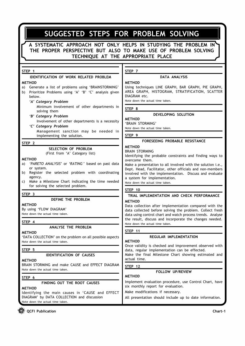
MILESTONE CHART - QUALITY CIRCLE ACTIVITY PLANNING
Project study planning is an effective method by which Quality Circle members
attain the skill to plan their activities and effective time management
QCFI Publication Chart-2
Quality Circle Name
Project
Project No.
Meeting Day
Time
Department Manager Facilitator Members' Name
Reason for selection
Date of beginning Date of completion
No. of projects completed
No. Activity Week 1 2 3 4 5 6 7 8 9 10 11 12 13 14 15 16 17 18 19 20 21 22 23 24
1. Defining the problem
2. Analyzing the problem
3. Identifying the causes
4. Finding out the rootcauses
5. Data analysis
7. Foreseeing possibleresistance
6. Developing solution
8. Trial implmn. andchecking performance
9. Regular Implmn.
10. Follow-up/Review
Target Actual

QCFI Publication Chart-3
GUIDELINES FOR CONSTRUCTING FLOW DIAGRAM
HIGH LEVEL FLOW DIAGRAM MATRIX FLOW DIAGRAM
DETAILED FLOW
DIAGRAM
WHEN TO DRAW FLOWDIAGRAMS?
1. For defining the
process flow.
2. For defining the
problem.
3. For identifying the
root causes.
4. For devising the
solution.
5. For implementing the
solution.
6. At the time of review/
follow up.
HOW TO DRAW A FLOWDIAGRAM?
Discuss the purpose of it.
Decide on your expectation.
Decide the boundaries.
Put each process in writingfrom the beginning.
When you come to adecision area follow one tillyou complete.
For unknown areas, checkup later on and complete.
Ensure every branch iscompleted.
Review it and ask othermembers also to review.
HOW TO ENSURE ACCURACY?
Ensure that it is about
actual process and not what
is intended.
Ensure rework loops are not
omitted.
Be honest about what you
do
Observe actual process
before drawing a Flow
diagram
Elicit support of other
members for accuracy and
completeness and allow
them to review it.
SYMBOLS USED IN
FLOW DIAGRAM?
Activity symbol Decision
symbol
Flow Lines Document
symbol
Data Base Connector
Start & End
USER SENDSINDENT
QUOTATIONOBTAINED
MATERIALORDERED
MATERIALRECEIVED
MATERIALMADE
INSPECTED USEROBTAINS
USER PURCHASE MANUFAC STORES INSPEC -TURER -TION
USER SENDSINDENT
QUOTATIONOBTAINED
MATERIALORDERED
MATERIALRECEIVED
MATERIALMADE
INSPECTED
USEROBTAINS
Flow Diagram is graphical or a pictorial way to depict a process. With the help of a flowdiagram we can show process sequence. It can be used to dissect a process for betterunderstanding and analysing. It can also be used for replanning or making a change.
The process may be a manufacturing process of a product (entire or segment), a serviceprovided, to convey some information or a combination of any of them.
START
Mtrl. needed
Mtrl. database
Is
it
there
Send Reqsn .
Mtrl.
Obtained
STOP
Raise Indent
Indent Recd.
Is it OK
Send Enqrs .
Qtn. OK
Return for correction
Place order
Mtrl. made
Mtrl. recd.
Inspection
Is it
OK
Take as stock
Put in
database
Return to supplier
Yes
Yes
No
No
YesNo
Yes
No
START
Mtrl. needed
Mtrl. database
Is
it
there
Send Reqsn .
Mtrl.
Obtained
STOP
Raise Indent
Indent Recd.
Is it OK
Send Enqrs .
Qtn. OK
Return for correction
Place order
Mtrl. made
Mtrl. recd.
Inspection
Is it
OK
Take as stock
Put in
database
Return to supplier
Yes
Yes
No
No
YesNo
Yes
No
QCFI Publication Chart-4
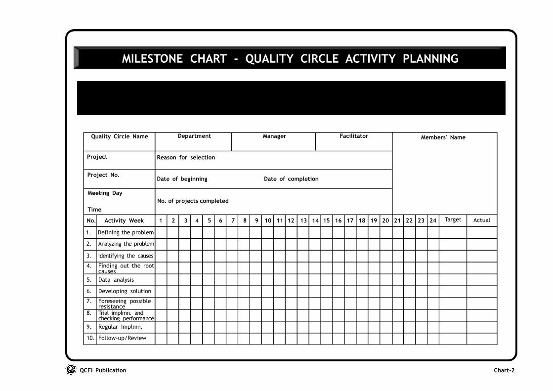
GUIDELINES FOR CONDUCTING BRAINSTORMING
Brainstorming is a group technique for generating new and usefulideas. It uses a few simple rules for discussion on a subject matter
that contributes to originality and innovation.
TYPES OF BRAINSTORMING
a. Free Wheeling or Unstructured
No hold, no bar system. No limit on
number of ideas at a time. It is
spontaneous and stimulates the
creativity of the individual.
b. Slip Method
When you need the involvement of
a large groups such method is used.
c. Round Robin or Structured
Quality Circle uses this system.
KEY ELEMENTS CONCERNING HUMANCREATIVE ABILITY
(JP GUILFORD’S RESEARCH FINDINGS)
FLUENCY
Capability of producing maximum ideas within
a given time.
FLEXIBILITY
Ability for the mind to move from one aspect
to another.
ORIGINALITY
Innovative or new ideas one can think of.
AWARENESS
Ability to look ahead into future.
DRIVE
Willingness to participate and contribute
without any hesitation.
GUIDELINES FORCONDUCTING BRAINSTORMINGIN A STRUCTURED MANNER
1. Keep the participants, preferably,
between six to ten.
2. Make it very clear to all the
participants on what subject the
Brainstorming is done.
3. Give required time for incubation.
4. Enter the points on a Black Board,
Flip Chart or in a Transparency for
all to see.
5. Explain the guidelines.
6. One idea only at a time.
7. Contribution in turn.
8. You may pass.
9. Clarify the point but don’t explain
the ideas.
10. No criticism. Encourage them to
do ‘hitch hiking’.
11. If session looses grip, have a break
or change.
12. To bring creativity use five Ws and
one H (When, Where, What, Who,
Why and How) appropriately.
13. Get maximum number of ideas.
14. Guests are welcome but will abide
by the rules.
15. Clarify each contribution.
16. Agree on a evaluation criteria.
QCFI Publication Chart-5
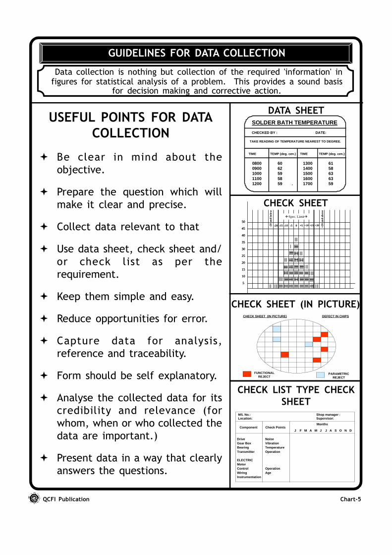
GUIDELINES FOR DATA COLLECTION
Data collection is nothing but collection of the required 'information' infigures for statistical analysis of a problem. This provides a sound basis
for decision making and corrective action.
SOLDER BATH TEMPERATURE
CHECKED BY : DATE:
TAKE READING OF TEMPERATURE NEAREST TO DEGREE.
TIME TEMP (deg. cen.) TIME TEMP (deg. cen.)
0800 60 1300 610900 62 1400 581000 59 1500 631100 58 1600 631200 59 . 1700 59
FUNCTIONALREJECT
PARAMETRICREJECT
CHECK SHEET (IN PICTURE) DEFECT IN CHIPS
USEFUL POINTS FOR DATACOLLECTION
� Be clear in mind about the
objective.
� Prepare the question which will
make it clear and precise.
� Collect data relevant to that
� Use data sheet, check sheet and/
or check list as per the
requirement.
� Keep them simple and easy.
� Reduce opportunities for error.
� Capture data for analysis,
reference and traceability.
� Form should be self explanatory.
� Analyse the collected data for its
credibility and relevance (for
whom, when or who collected the
data are important.)
� Present data in a way that clearly
answers the questions.
DATA SHEET
CHECK SHEET
CHECK SHEET (IN PICTURE)
M/L No.: Shop manager :Location: Supervisor:
Component Check PointsMonths
J F M A M J J A S O N D
Drive NoiseGear Box VibrationBearing TemperatureTransmitter Operation
ELECTRICMotorControl OperationWiring AgeInstrumentation
CHECK LIST TYPE CHECKSHEET
5
10
15
20
25
30
35
40
45
50
-20
and
bel
ow
-20 -15 -10 -5 0 +5 +10 +15 +20 +20
and
abo
ve
�Spec. Limit�
5
10
15
20
25
30
35
40
45
50
-20
and
bel
ow
-20 -15 -10 -5 0 +5 +10 +15 +20 +20
and
abo
ve
�Spec. Limit�
QCFI Publication Chart-6
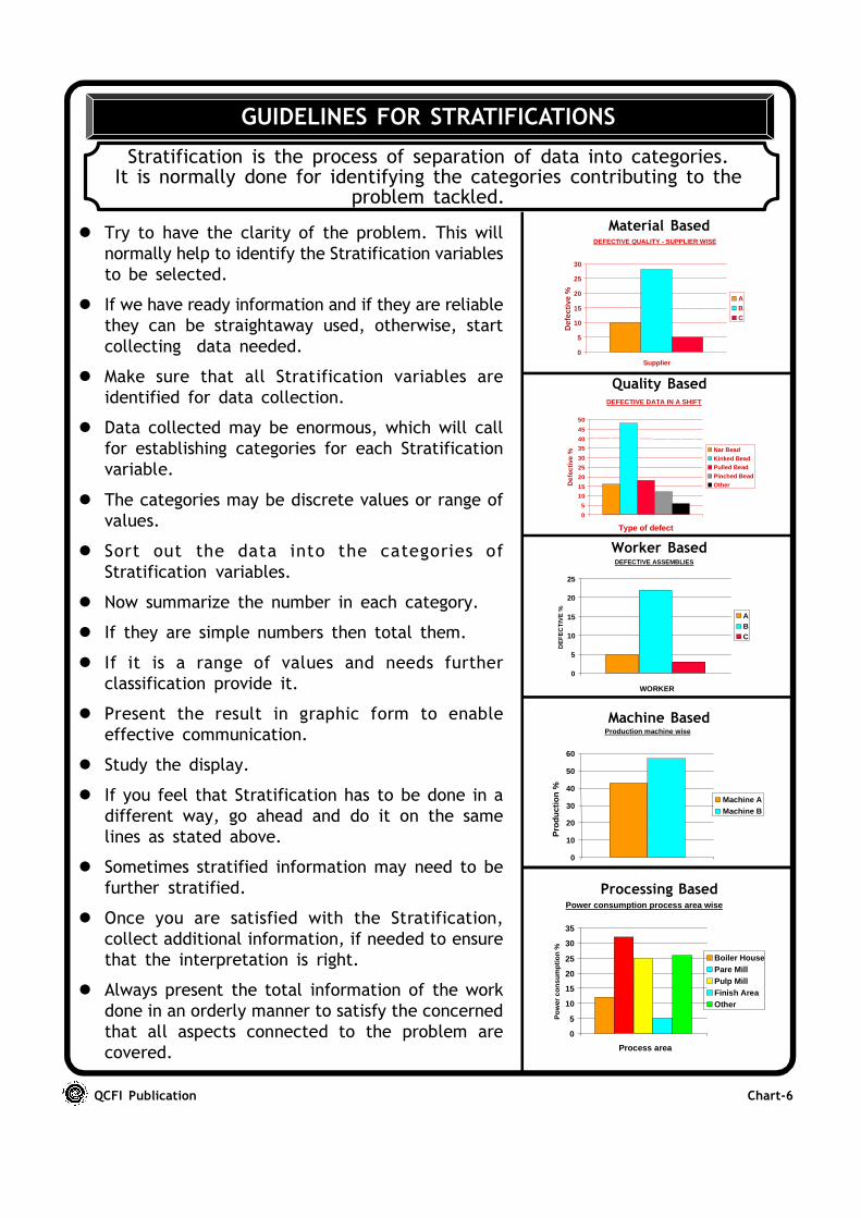
GUIDELINES FOR STRATIFICATIONS
Stratification is the process of separation of data into categories.It is normally done for identifying the categories contributing to the
problem tackled.
� Try to have the clarity of the problem. This will
normally help to identify the Stratification variables
to be selected.
� If we have ready information and if they are reliable
they can be straightaway used, otherwise, start
collecting data needed.
� Make sure that all Stratification variables are
identified for data collection.
� Data collected may be enormous, which will call
for establishing categories for each Stratification
variable.
� The categories may be discrete values or range of
values.
� Sort out the data into the categories of
Stratification variables.
� Now summarize the number in each category.
� If they are simple numbers then total them.
� If it is a range of values and needs further
classification provide it.
� Present the result in graphic form to enable
effective communication.
� Study the display.
� If you feel that Stratification has to be done in a
different way, go ahead and do it on the same
lines as stated above.
� Sometimes stratified information may need to be
further stratified.
� Once you are satisfied with the Stratification,
collect additional information, if needed to ensure
that the interpretation is right.
� Always present the total information of the work
done in an orderly manner to satisfy the concerned
that all aspects connected to the problem are
covered.
0
5
10
15
20
25
30
Supplier
ABC
Def
ectiv
e %
DEFECTIVE QUALITY - SUPPLIER WISE
0
5
10
15
20
25
30
35
40
45
50
Nar BeadKinked BeadPulled BeadPinched BeadOther
Type of defect
Def
ecti
ve %
DEFECTIVE DATA IN A SHIFT
0
5
10
15
20
25
ABC
WORKER
DE
FE
CT
IVE
%DEFECTIVE ASSEMBLIES
0
10
20
30
40
50
60
Machine AMachine B
Pro
duct
ion
%
Production machine wise
0
5
10
15
20
25
30
35
Boiler HousePare MillPulp MillFinish AreaOther
Process area
Pow
er c
onsu
mpt
ion
%
Power consumption process area wise
Material Based
Quality Based
Worker Based
Machine Based
Processing Based
QCFI Publication Chart-7
USEFUL POINTS FORMAKING GRAPH
� Be clear on the purpose of
making a graph
� Arrange the information in order
� Decide on the type of graph
� Decide on the title
� Show the data
� Substance is more important
than method. Good graphs are
those which draw attention to
data
� Avoid distorting the information
� Make it easier for eyes to
compare
� Large amount of data should be
depicted in summary form and
then into finer details
� Let graph serve a clear purpose
of exploration, tabulation or
decoration
� Should be closely integrated
with statistical and verbal
descriptions of a data set.
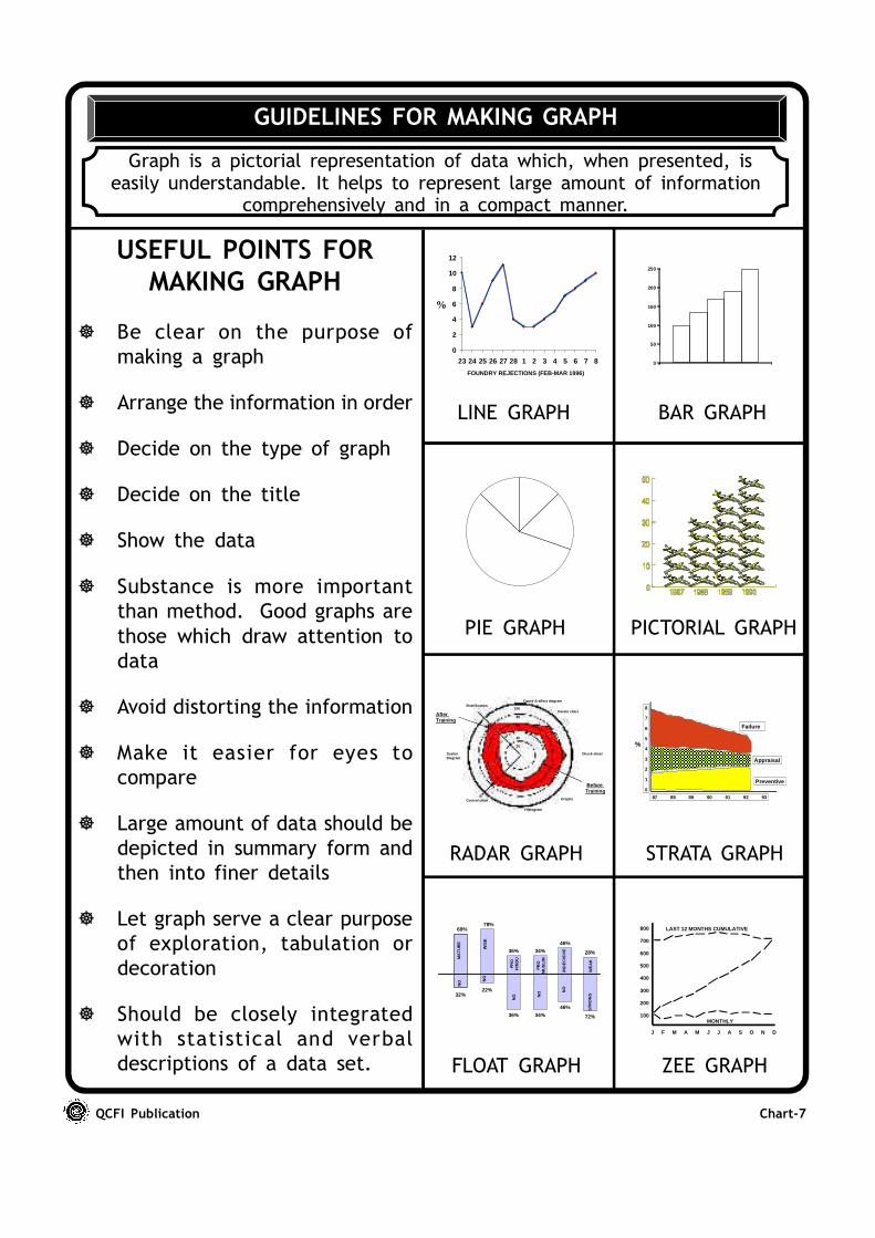
GUIDELINES FOR MAKING GRAPH
Graph is a pictorial representation of data which, when presented, iseasily understandable. It helps to represent large amount of information
comprehensively and in a compact manner.
0
2
4
6
8
10
12
23 24 25 26 27 28 1 2 3 4 5 6 7 8
FOUNDRY REJECTIONS (FEB-MAR 1996)
%
0
50
100
150
200
250
Cause & effect diagram
Pareto chart
Check sheet
Graphs
Histogram
Control chart
ScatterDiagram
Stratification100
80
60
40
20
After Training
Before Training
8
7
6
5
4
3
2
1
0
87 88 89 90 91 92 93
Failure
Appraisal
Preventive
%
MA
TU
RE
WIS
E
PR
OH
IND
U
PR
OM
US
LIM
STR
ON
GW
EA
K
NO N
O
NO N
O NO
IND
EC
ISIV
E
68%78%
36% 34%
46%
28%
32%22%
36% 34%
46%
72%
J F M A M J J A S O N D
800
700
600
500
400
300
200
100MONTHLY
LAST 12 MONTHS CUMULATIVE
LINE GRAPH BAR GRAPH
PIE GRAPH PICTORIAL GRAPH
RADAR GRAPH STRATA GRAPH
FLOAT GRAPH ZEE GRAPH
QCFI Publication Chart-8
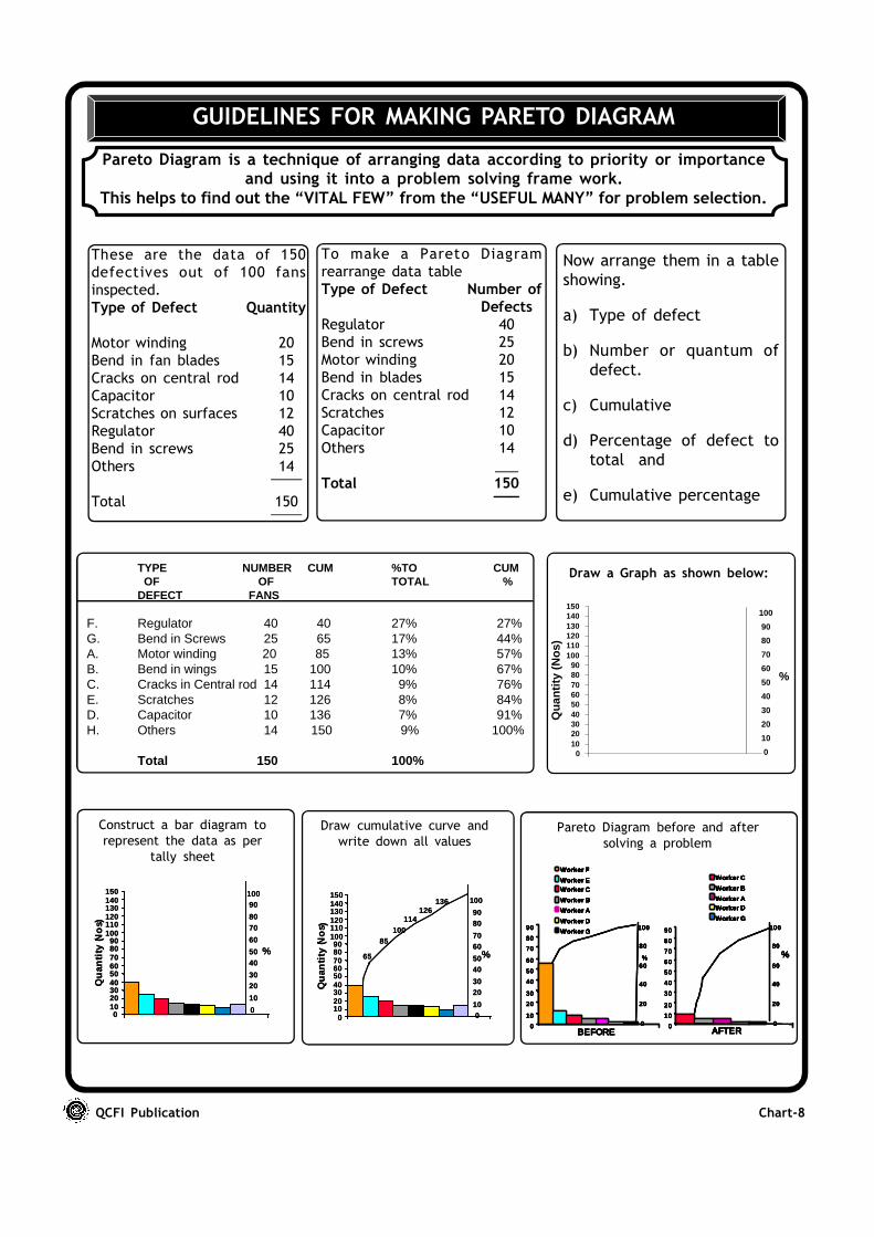
GUIDELINES FOR MAKING PARETO DIAGRAM
Pareto Diagram is a technique of arranging data according to priority or importanceand using it into a problem solving frame work.
This helps to find out the “VITAL FEW” from the “USEFUL MANY” for problem selection.
These are the data of 150
defectives out of 100 fans
inspected.
Type of Defect Quantity
Motor winding 20
Bend in fan blades 15
Cracks on central rod 14
Capacitor 10
Scratches on surfaces 12
Regulator 40
Bend in screws 25
Others 14____
Total 150____
To make a Pareto Diagram
rearrange data table
Type of Defect Number ofDefects
Regulator 40
Bend in screws 25
Motor winding 20
Bend in blades 15
Cracks on central rod 14
Scratches 12
Capacitor 10
Others 14
___
Total 150___
Now arrange them in a table
showing.
a) Type of defect
b) Number or quantum of
defect.
c) Cumulative
d) Percentage of defect to
total and
e) Cumulative percentage
TYPE NUMBER CUM %TO CUM OF OF TOTAL %DEFECT FANS
F. Regulator 40 40 27% 27%G. Bend in Screws 25 65 17% 44%A. Motor winding 20 85 13% 57%B. Bend in wings 15 100 10% 67%C. Cracks in Central rod 14 114 9% 76%E. Scratches 12 126 8% 84%D. Capacitor 10 136 7% 91%H. Others 14 150 9% 100%
Total 150 100%0
102030405060708090
100110120130140150
100
90
80
70
60
50
40
30
20
10
0
%
Qu
anti
ty (
No
s)
Draw a Graph as shown below:
Construct a bar diagram to
represent the data as per
tally sheet
Draw cumulative curve and
write down all valuesPareto Diagram before and after
solving a problem
0102030405060708090
100110120130140150 100
90
8070
60
5040
3020
10
0
%
Qu
anti
ty (N
os)
0102030405060708090
100110120130140150 100
90
8070
60
5040
3020
10
0
%
Qu
anti
ty (N
os)
0102030405060708090
100110120130140150
65
85100
114126
136 100
9080
7060
5040
3020
100
%
Qu
anti
ty (N
os )
0102030405060708090
100110120130140150
65
85100
114126
136 100
9080
7060
5040
3020
100
%
Qu
anti
ty (N
os )
Worker F
Worker EWorker C
Worker B
Worker A
Worker D
Worker G
0
10
20
30
40
50
60
70
80
90 100
80
60
40
20
0
%
BEFORE
Worker C
Worker B
Worker AWorker D
Worker G
0
10
20
30
40
50
60
70
80
90
AFTER
100
80
60
40
20
0
%
Worker F
Worker EWorker C
Worker B
Worker A
Worker D
Worker G
Worker F
Worker EWorker C
Worker B
Worker A
Worker D
Worker G
0
10
20
30
40
50
60
70
80
90 100
80
60
40
20
0
%
BEFORE
Worker C
Worker B
Worker AWorker D
Worker G
Worker C
Worker B
Worker AWorker D
Worker G
0
10
20
30
40
50
60
70
80
90
AFTER
100
80
60
40
20
0
%
Worker F
Worker EWorker C
Worker B
Worker A
Worker D
Worker G
0
10
20
30
40
50
60
70
80
90 100
80
60
40
20
0
%
BEFORE
Worker C
Worker B
Worker AWorker D
Worker G
0
10
20
30
40
50
60
70
80
90
AFTER
100
80
60
40
20
0
%
Worker F
Worker EWorker C
Worker B
Worker A
Worker D
Worker G
Worker F
Worker EWorker C
Worker B
Worker A
Worker D
Worker G
0
10
20
30
40
50
60
70
80
90 100
80
60
40
20
0
%
BEFORE
Worker C
Worker B
Worker AWorker D
Worker G
Worker C
Worker B
Worker AWorker D
Worker G
0
10
20
30
40
50
60
70
80
90
AFTER
100
80
60
40
20
0
%
QCFI Publication Chart-9
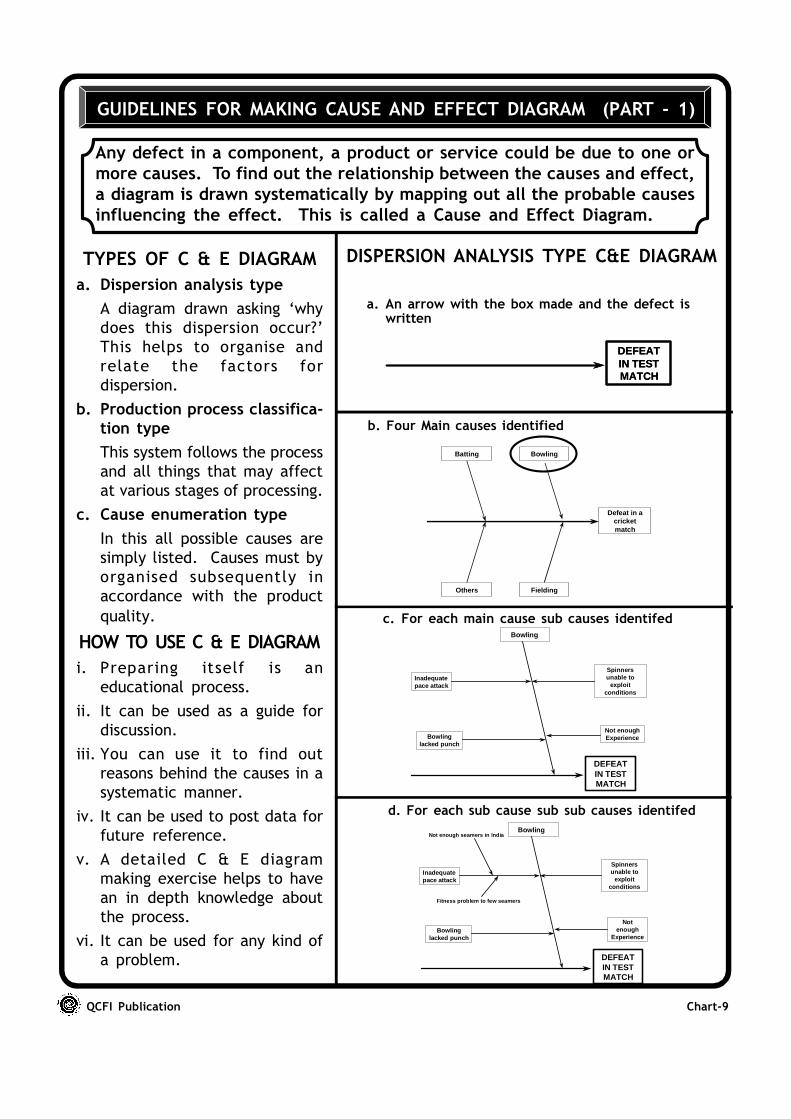
Any defect in a component, a product or service could be due to one ormore causes. To find out the relationship between the causes and effect,a diagram is drawn systematically by mapping out all the probable causesinfluencing the effect. This is called a Cause and Effect Diagram.
TYPES OF C & E DIAGRAM
a. Dispersion analysis type
A diagram drawn asking ‘why
does this dispersion occur?’
This helps to organise and
relate the factors for
dispersion.
b. Production process classifica-tion type
This system follows the process
and all things that may affect
at various stages of processing.
c. Cause enumeration type
In this all possible causes are
simply listed. Causes must by
organised subsequently in
accordance with the product
quality.
HOW TO USE C & E DIAGRAM
i. Preparing itself is an
educational process.
ii. It can be used as a guide for
discussion.
iii. You can use it to find out
reasons behind the causes in a
systematic manner.
iv. It can be used to post data for
future reference.
v. A detailed C & E diagram
making exercise helps to have
an in depth knowledge about
the process.
vi. It can be used for any kind of
a problem.
DISPERSION ANALYSIS TYPE C&E DIAGRAM
d. For each sub cause sub sub causes identifed
c. For each main cause sub causes identifed
Defeat in acricketmatch
Batting Bowling
FieldingOthers
b. Four Main causes identified
a. An arrow with the box made and the defect iswritten
GUIDELINES FOR MAKING CAUSE AND EFFECT DIAGRAM (PART - 1)
DEFEAT IN TEST MATCH
Bowling
Inadequate pace attack
Spinners unable to
exploit conditions
Bowling lacked punch
Not enough Experience
DEFEAT IN TEST MATCH
Bowling
Inadequate pace attack
Spinners unable to
exploit conditions
Bowling lacked punch
Not enough
Experience
Not enough seamers in India
Fitness problem to few seamers
DEFEAT IN TEST MATCH
DEFEAT IN TEST MATCH
QCFI Publication Chart-10
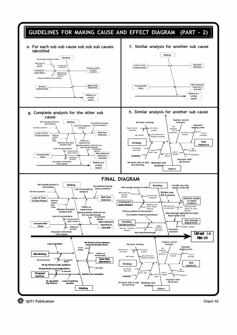
GUIDELINES FOR MAKING CAUSE AND EFFECT DIAGRAM (PART - 2)
Defeat in acricketmatch
Batting
Lack of Tech.To face Pacers
Not enough practice infast wickets
Batsmen lack goodbackfoot tech.
Differentwicketsbackhome
No time to practice
Bad teamSelection
Lack of foresight byselectors
Politics atregional level
Few batsmen havingfitness problems
Irresponsibleshots
Lack of concentration
No proper instructionsfrom Captain
Unsure of hisplace in team
Infighing inthe team
Main batsmenexposed to
new ball
Opening batters could not seethe new ball through
No specialistopeners
g. Complete analysis for the other subcause
Defeat in acricketmatch
Bowling
Inadequatepace attack
Not enough seamers in India
Indian pitch donot helpseamers
Very few Paceacademies
Fitness problem to few seamers
Bowling in netwithout properwarm up.
Spinners unableto exploit
conditions
Bowlinglacked punch
Not enoughExperience
e. For each sub sub cause sub sub sub causesidentifed
Defeat in acricketmatch
Batting
Lack of Tech.To face Pacers
Bad teamSelection
Irresponsibleshots
Main batsmenexposed to
new ball
f. Similar analysis for another sub cause
Def eatDef eatDef eatDef eat i ni ni ni n Mat chMat chMat chMat ch
Batting
Lack of Tech.To face Pacers
Not enough practice infast wickets
Batsmen lack goodbackfoot tech.
Differentwicketsbackhome
No time to practice
Bad teamSelection
Lack of foresight byselectors
Politics atregional level
Few batsmen havingfitness problems
Irresponsibleshots
Lack of concentration
No proper instructionsfrom Captain
Unsure of hisplace in team
Infighing inthe team
Main batsmenexposed to
new ball
Opening batters could not seethe new ball through
No specialistopeners
FINAL DIAGRAM
h. Similar analysis for another sub cause
Strategy
Improper fieldplacement
Improperbatting order
Captain cannotmotivate
Notrespected
byteammates Lot of new
batsmenLack of
foresight
Immaturity
Egoproblems
Lack ofstrategy
No basic strategy
Players do notcontribute
ego hassles
No time toprepare
No professionalstrategist consulted
No game plan to playfast bowling
Batsmen notstudied
Inability
No batsmentakes lead Lack of
proff . helpLack of
Videos
Badcaptaincy
Others
Mis-fielding
Lack of practice
No specialistfielders
Bad field Placement
No Sp. Fielders atSp. positions
Wrong fielders at wrongpositionsNo game plan
Droppedcatches
No specialistslip fielders
Lack of catchingpractice
Bowlers not consulted
ego hassles
Bad fieldplacement
No fielders where batsmenplays his favorite shots
Lack of
strategy
Batsmen not
studied properly
Fielding
Bowling
Inadequatepace attack
Spinners unableto exploitconditions
Kumble not a bigspinner of the ball
Wicket wasflat & grassy
Not enough spinners in team
Bowlinglacked punch
Main bowlers sick
Bad teamselectionNot motivated enough
Few bowlers lacked commitment
Not enough seamers in India
Fitness problem to fewseamers
Most sp in nersin a bad patch
Had to sacr ificespinner for extrabatsmen
Not enoughExperience
Regoina l po liticsHighlymotivatedoppos itio n
Flat track Frustatedspinners
Ind ian pitch d onot he lpseamers
Very few Paceacademies
Bowling in netwithot properwarm up.
QCFI Publication Chart-11
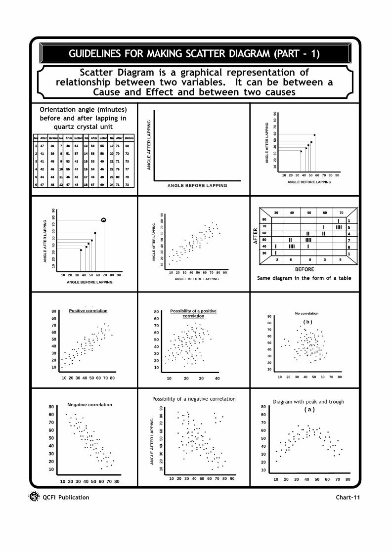
GUIDELINES FOR MAKING SCATTER DIAGRAM (PART - 1)
Scatter Diagram is a graphical representation ofrelationship between two variables. It can be between a
Cause and Effect and between two causes
ANGLE BEFORE LAPPING
AN
GLE
AF
TE
R L
AP
PIN
G
ANGLE BEFORE LAPPING
AN
GLE
AF
TE
R L
AP
PIN
G
10 20 30 40 50 60 70 80 90
10
20
30
40
50
60
70
80
90
. ....
ANGLE BEFORE LAPPING
AN
GLE
AF
TE
R L
AP
PIN
G
10 20 30 40 50 60 70 80 90
10
20
30
40
50
60
70
80
90
. ....
.
ANGLE BEFORE LAPPING
AN
GLE
AF
TE
R L
AP
PIN
G
10 20 30 40 50 60 70 80 90
10
20
30
40
50
60
70
80
90
( a )
10 20 30 40 50 60 70 80
80
60
70
60
50
40
30
20
10
Positive correlation
10 20 30 40 50 60 70 80
80
60
70
60
50
40
30
20
10
( a )
( b )
10 20 30 40 50 60 70 80
80
60
70
60
50
40
30
20
10
Negative correlation
AN
GLE
AF
TE
R L
AP
PIN
G
10 20 30 40 50 60 70 80 90
10
20
30
40
50
60
70
80
90
Possibility of a positivecorrelation
80
60
70
60
50
40
30
20
10
10 20 30 40
Orientation angle (minutes)
before and after lapping in
quartz crystal unit
Same diagram in the form of a table
BEFORE
AFTER
10 20 30 40 50 60 70 80
80
60
70
60
50
40
30
20
10
No correlation
( b )
Possibility of a negative correlationDiagram with peak and trough
No After Before No After Before No After Before No After Before
1 37 36
2 41 39
3 41 45
4 42 46
5 44 44
6 47 48
7 48 51
8 51 57
9 53 42
10 55 47
11 46 48
12 47 48
13 58 55
14 58 58
15 53 49
16 54 46
17 46 48
18 67 69
19 71 68
20 70 72
21 71 73
22 76 77
23 80 70
24 71 73
No After Before No After Before No After Before No After Before
1 37 36
2 41 39
3 41 45
4 42 46
5 44 44
6 47 48
7 48 51
8 51 57
9 53 42
10 55 47
11 46 48
12 47 48
13 58 55
14 58 58
15 53 49
16 54 46
17 46 48
18 67 69
19 71 68
20 70 72
21 71 73
22 76 77
23 80 70
24 71 73
80
70
60
50
40
30
30 40 50 60 70
I
II
IIIIII
III
IIIIIII
IIII
2 6 8 3 5
1
5
4
7
6
1
80
70
60
50
40
30
30 40 50 60 70
I
II
IIIIII
III
IIIIIII
IIII
2 6 8 3 5
1
5
4
7
6
1
QCFI Publication Chart-12
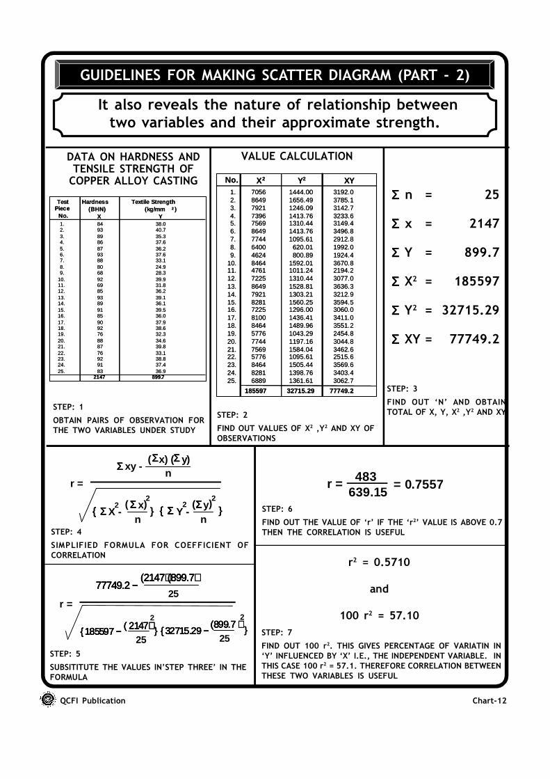
GUIDELINES FOR MAKING SCATTER DIAGRAM (PART - 2)
It also reveals the nature of relationship betweentwo variables and their approximate strength.
Σ Σ Σ Σ n = 25
Σ Σ Σ Σ x = 2147
Σ Σ Σ Σ Y = 899.7
Σ Σ Σ Σ X2 = 185597
Σ Σ Σ Σ Y2 = 32715.29
Σ Σ Σ Σ XY = 77749.2
DATA ON HARDNESS ANDTENSILE STRENGTH OFCOPPER ALLOY CASTING
STEP: 1
OBTAIN PAIRS OF OBSERVATION FOR
THE TWO VARIABLES UNDER STUDY
VALUE CALCULATION
STEP: 2
FIND OUT VALUES OF X2 ,Y2 AND XY OF
OBSERVATIONS
STEP: 3
FIND OUT ‘N’ AND OBTAIN
TOTAL OF X, Y, X2 ,Y2 AND XY
STEP: 4
SIMPLIFIED FORMULA FOR COEFFICIENT OF
CORRELATION
STEP: 5
SUBSITITUTE THE VALUES IN’STEP THREE’ IN THE
FORMULA
STEP: 6
FIND OUT THE VALUE OF ‘r’ IF THE ‘r2’ VALUE IS ABOVE 0.7
THEN THE CORRELATION IS USEFUL
r2 = 0.5710
and
100 r2 = 57.10
STEP: 7
FIND OUT 100 r2. THIS GIVES PERCENTAGE OF VARIATIN IN
‘Y’ INFLUENCED BY ‘X’ I.E., THE INDEPENDENT VARIABLE. IN
THIS CASE 100 r2 = 57.1. THEREFORE CORRELATION BETWEEN
THESE TWO VARIABLES IS USEFUL
483= 0.7557
639.15r =r =
ΣΣΣΣ xy -(ΣΣΣΣx) (ΣΣΣΣ y)
n
2
{ Σ { Σ { Σ { Σ X -ΣΣΣΣ x) ΣΣΣΣ y)
n n2
2( { Σ { Σ { Σ { Σ Y -
2}
(}
r =
(2147) (899.7)(2147) (899.7)(2147) (899.7)(2147) (899.7)25
( 2147) ( 2147) ( 2147) ( 2147) } (899.7 ) (899.7 ) (899.7 ) (899.7 )
}25 25
2 2
77749.2 −77749.2 −77749.2 −77749.2 −
{185597 −{185597 −{185597 −{185597 − {32715.29 −{32715.29 −{32715.29 −{32715.29 −
TestPiece
No.
Hardness(BHN)
X
Textile Strength(kg/mm 2 )
Y1. 84 38.02. 93 40.73. 89 35.34. 86 37.65. 87 36.26. 93 37.67. 88 33.18. 80 24.99. 68 28.3
10. 92 39.911. 69 31.812. 85 36.213. 93 39.114. 89 36.115. 91 39.516. 85 36.017. 90 37.918. 92 38.619. 76 32.320. 88 34.621. 87 39.822. 76 33.123. 92 38.824. 91 37.425. 83 36.9
2147 899.7
No. X2 Y2
1. 7056 1444.00 3192.02. 8649 1656.49 3785.13. 7921 1246.09 3142.74. 7396 1413.76 3233.65. 7569 1310.44 3149.46. 8649 1413.76 3496.87. 7744 1095.61 2912.88. 6400 620.01 1992.09. 4624 800.89 1924.4
10. 8464 1592.01 3670.811. 4761 1011.24 2194.212. 7225 1310.44 3077.013. 8649 1528.81 3636.314. 7921 1303.21 3212.915. 8281 1560.25 3594.516. 7225 1296.00 3060.017. 8100 1436.41 3411.018. 8464 1489.96 3551.219. 5776 1043.29 2454.820. 7744 1197.16 3044.821. 7569 1584.04 3462.622. 5776 1095.61 2515.623. 8464 1505.44 3569.624. 8281 1398.76 3403.425. 6889 1361.61 3062.7
185597 32715.29 77749.2
XYNo. X2 Y2
1. 7056 1444.00 3192.02. 8649 1656.49 3785.13. 7921 1246.09 3142.74. 7396 1413.76 3233.65. 7569 1310.44 3149.46. 8649 1413.76 3496.87. 7744 1095.61 2912.88. 6400 620.01 1992.09. 4624 800.89 1924.4
10. 8464 1592.01 3670.811. 4761 1011.24 2194.212. 7225 1310.44 3077.013. 8649 1528.81 3636.314. 7921 1303.21 3212.915. 8281 1560.25 3594.516. 7225 1296.00 3060.017. 8100 1436.41 3411.018. 8464 1489.96 3551.219. 5776 1043.29 2454.820. 7744 1197.16 3044.821. 7569 1584.04 3462.622. 5776 1095.61 2515.623. 8464 1505.44 3569.624. 8281 1398.76 3403.425. 6889 1361.61 3062.7
185597 32715.29 77749.2
XY
QCFI Publication Chart-13
GUIDELINES FOR MAKING HISTOGRAM
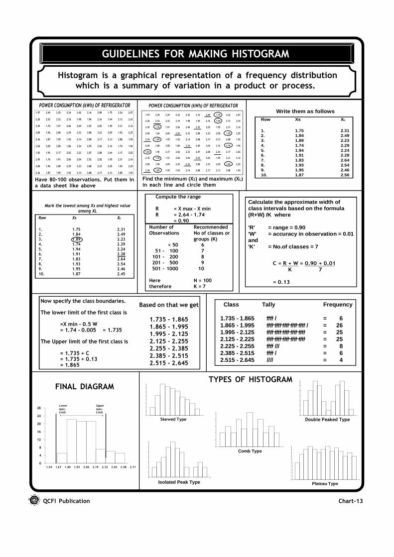
Histogram is a graphical representation of a frequency distributionwhich is a summary of variation in a product or process.
1.97 2.49 2.29 2.24 2.42 2.16 2.89 1.75 2.24 2.07
2.20 2.52 2.32 2.10 1.98 1.96 2.16 1.94 2.13 2.43
2.45 1.76 1.91 2.06 2.04 2.52 2.02 1.95 2.31 2.16
2.00 1.96 2.00 2.29 2.33 2.08 2.23 2.05 1.92 2.25
2.36 1.87 1.95 1.92 2.14 2.08 2.17 2.13 2.08 1.92
2.04 2.00 2.08 1.86 2.34 2.05 2.04 2.16 1.74 1.96
1.83 1.95 2.17 2.02 2.23 2.07 2.08 2.64 2.17 2.02
2.45 1.76 1.91 2.06 2.04 2.52 2.02 1.95 2.31 2.16
2.00 1.96 2.00 2.29 2.33 2.08 2.23 2.05 1.92 2.25
2.36 1.87 1.95 1.92 2.14 2.08 2.17 2.13 2.08 1.92
POWER CONSUMPTION (kWh) OF REFRIGERATOR
Mark the lowest among Xs and highest valueamong XL
RowRow XsXs XXLL
1. 1.75 2.312. 1.84 2.493. 1.89 2.23
4. 1.74 2.295. 1.94 2.246. 1.91 2.287. 1.83 2.648. 1.93 2.549. 1.95 2.4610. 1.87 2.45
Calculate the approximate width ofclass intervals based on the formula(R+W) /K where
'R' = range = 0.90'W' = accuracy in observation = 0.01and'K' = No.of classes = 7
C = R + W = 0.90 + 0.01
K 7
= 0.13
Now specify the class boundaries.
The lower limit of the first class is
=X min - 0.5 W= 1.74 - 0.005 = 1.735
The Upper limit of the first class is
= 1.735 + C= 1.735 + 0.13= 1.865
Based on that we get
1.735 - 1.8651.865 - 1.9951.995 - 2.1252.125 - 2.2552.255 - 2.3852.385 - 2.5152.515 - 2.645
Class Tally Frequency
1.735 - 1.865 //// / = 61.865 - 1.995 //// //// //// //// //// / = 261.995 - 2.125 //// //// //// //// //// = 252.125 - 2.225 //// //// //// //// //// = 252.225 - 2.255 //// /// = 82.385 - 2.515 //// / = 62.515 - 2.645 //// = 4
Have 80-100 observations. Put them ina data sheet like above
Find the minimum (XS) and maximum (XL)in each line and circle them
Write them as follows
RowRow XsXs XXLL
1. 1.75 2.312. 1.84 2.493. 1.89 2.234. 1.74 2.295. 1.94 2.246. 1.91 2.287. 1.83 2.648. 1.93 2.549. 1.95 2.4610. 1.87 2.56
Number of RecommendedObservations No of classes or
groups (K)< 50 6
51 - 100 7 101 - 200 8 201 - 500 9 501 - 1000 10
Here N = 100therefore K = 7
Compute the range
R = X max - X minR = 2.64 - 1.74 = 0.90
0
4
8
12
16
20
24
28
1.54 1.67 1.80 1.93 2.06 2.19 2.32 2.45 2.58 2.71
Lower
spec.Limit
Upper
spec.Limit
FINAL DIAGRAMTYPES OF HISTOGRAM
Skewed Type Double Peaked Type
Comb Type
Isolated Peak Type Plateau Type
QCFI Publication Chart-14
GUIDELINES FOR CONSTRUCTING CONTROL CHART (PART - 1)
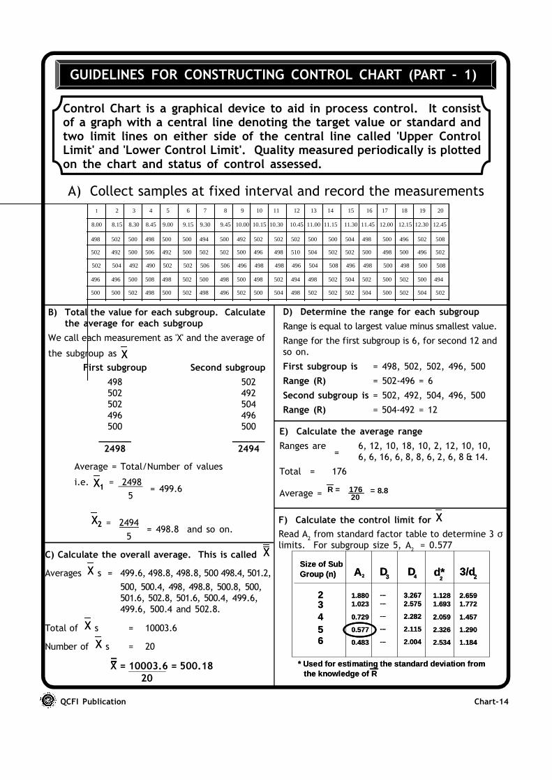
Control Chart is a graphical device to aid in process control. It consistof a graph with a central line denoting the target value or standard andtwo limit lines on either side of the central line called 'Upper ControlLimit' and 'Lower Control Limit'. Quality measured periodically is plottedon the chart and status of control assessed.
498 502 500 498 500 500 494 500 492 502 502 502 500 500 504 498 500 496 502 508
8.00 8.15 8.30 8.45 9.00 9.15 9.30 9.45 10.00 10.15 10.30 10.45 11.00 11.15 11.30 11.45 12.00 12.15 12.30 12.45
502 492 500 506 492 500 502 502 500 496 498 510 504 502 502 500 498 500 496 502
502 504 492 490 502 502 506 506 496 498 498 496 504 508 496 498 500 498 500 508
496 496 500 508 498 502 500 498 500 498 502 494 498 502 504 502 500 502 500 494
500 500 502 498 500 502 498 496 502 500 504 498 502 502 502 504 500 502 504 502
1 2 3 4 5 6 7 8 9 10 11 12 13 14 15 16 17 18 19 20
A) Collect samples at fixed interval and record the measurements
B) Total the value for each subgroup. Calculatethe average for each subgroup
We call each measurement as 'X' and the average of
the subgroup as XXFirst subgroup Second subgroup
498 502
502 492
502 504
496 496
500 500
______ ______2498 2494
Average = Total/Number of values
i.e. X1X1 = 2498
= 499.6
_____
5
X2X2 = 2494 = 498.8 and so on.
____
5
C) Calculate the overall average. This is called XX
Averages XX s = 499.6, 498.8, 498.8, 500 498.4, 501.2,
500, 500.4, 498, 498.8, 500.8, 500,
501.6, 502.8, 501.6, 500.4, 499.6,
499.6, 500.4 and 502.8.
Total of XX s = 10003.6
Number of XX s = 20
X = 10003.6 = 500.18 20
=
D) Determine the range for each subgroup
Range is equal to largest value minus smallest value.
Range for the first subgroup is 6, for second 12 and
so on.
First subgroup is = 498, 502, 502, 496, 500
Range (R) = 502-496 = 6
Second subgroup is = 502, 492, 504, 496, 500
Range (R) = 504-492 = 12
E) Calculate the average range
Ranges are =
6, 12, 10, 18, 10, 2, 12, 10, 10,
6, 6, 16, 6, 8, 8, 6, 2, 6, 8 & 14.
Total = 176
Average = R = 176 = 8.8 20
F) Calculate the control limit for XX
Read A2 from standard factor table to determine 3 σ
limits. For subgroup size 5, A2 = 0.577
* Used for estimating the standard deviation fromthe knowledge of R
2 1.880 --- 3.267 1.128 2.6593 1.023 --- 2.575 1.693 1.772
4 0.729 --- 2.282 2.059 1.457
5 0.577 --- 2.115 2.326 1.290
6 0.483 --- 2.004 2.534 1.184
D3
D4A2 d*2
3/d2
Size of SubGroup (n)
* Used for estimating the standard deviation fromthe knowledge of R
2 1.880 --- 3.267 1.128 2.6593 1.023 --- 2.575 1.693 1.772
4 0.729 --- 2.282 2.059 1.457
5 0.577 --- 2.115 2.326 1.290
6 0.483 --- 2.004 2.534 1.184
D3
D4A2 d*2
3/d2
Size of SubGroup (n)
QCFI Publication Chart-15
GUIDELINES FOR CONSTRUCTING CONTROL CHART (PART - 2)
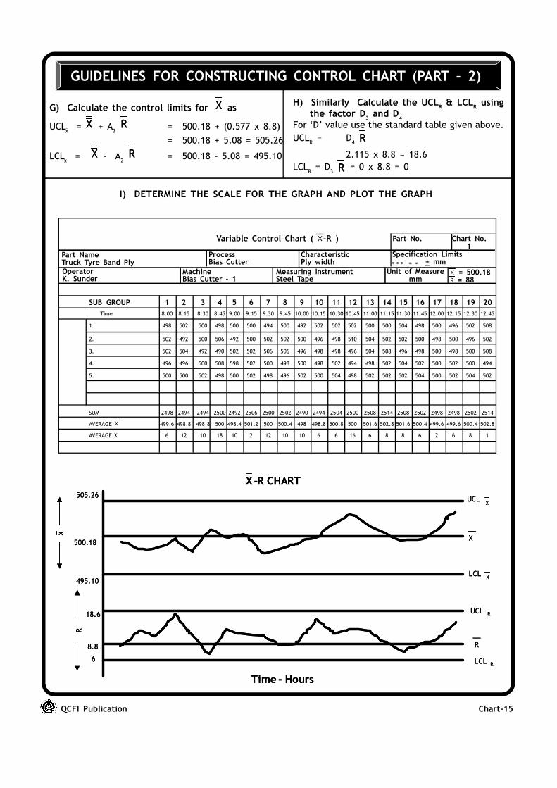
G) Calculate the control limits for XX as
UCL–x = XX + A
2
RR = 500.18 + (0.577 x 8.8)
= 500.18 + 5.08 = 505.26
LCL–x = XX - A
2
RR = 500.18 - 5.08 = 495.10
H) Similarly Calculate the UCLR & LCL
R using
the factor D3 and D
4
For ‘D’ value use the standard table given above.
UCLR = D
4 RR
2.115 x 8.8 = 18.6
LCLR = D
3 RR = 0 x 8.8 = 0
I) DETERMINE THE SCALE FOR THE GRAPH AND PLOT THE GRAPH
Variable Control Chart ( X-R ) Part No. Chart No.1
Specification Limits5 0 0 m m + mm
CharacteristicPly width
ProcessBias Cutter
Part NameTruck Tyre Band Ply
OperatorK. Sunder
SUB GROUP 1 2 3 4 5 6 7 8 9 10 11 12 13 14 15 16 17 18 19 20
Time 8.00 8.15 8.30 8.45 9.00 9.15 9.30 9.45 10.00 10.15 10.30 10.45 11.00 11.15 11.30 11.45 12.00 12.15 12.30 12.45
1. 498 502 500 498 500 500 494 500 492 502 502 502 500 500 504 498 500 496 502 508
2. 502 492 500 506 492 500 502 502 500 496 498 510 504 502 502 500 498 500 496 502
3. 502 504 492 490 502 502 506 506 496 498 498 496 504 508 496 498 500 498 500 508
4. 496 496 500 508 598 502 500 498 500 498 502 494 498 502 504 502 500 502 500 494
5. 500 500 502 498 500 502 498 496 502 500 504 498 502 502 502 504 500 502 504 502
SUM 2498 2494 2494 2500 2492 2506 2500 2502 2490 2494 2504 2500 2508 2514 2508 2502 2498 2498 2502 2514
AVERAGE X 499.6 498.8 498.8 500 498.4 501.2 500 500.4 498 498.8 500.8 500 501.6 502.8 501.6 500.4 499.6 499.6 500.4 502.8
AVERAGE X 6 12 10 18 10 2 12 10 10 6 6 16 6 8 8 6 2 6 8 1
MachineBias Cutter - 1
Measuring InstrumentSteel Tape
Unit of Measuremm
X = 500.18R = 88
505.26
500.18
495.10
18.6
6
x
R
LCL
LCL
X
X-R CHART
Time - Hours
8.8 R
R
UCL R
X
UCLX
505.26
500.18
495.10
18.6
6
x
R
LCL
LCL
X
X-R CHART
Time - Hours
8.8 R
R
UCL R
X
UCLX
QCFI Publication Chart-16
GUIDELINES FOR CONSTRUCTING CONTROL CHART (PART - 3)
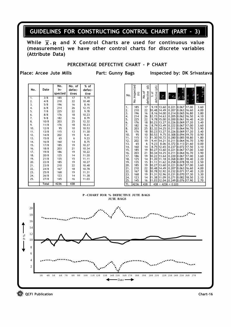
While X - R and X Control Charts are used for continuous value(measurement) we have other control charts for discrete variables(Attribute Data)
1. 3/8 185 17 9.19
2. 4/8 210 22 10.48
3. 5/8 196 16 8.16
4. 6/8 214 26 12.15
5. 7/8 225 22 9.78
6. 8/8 176 18 10.23
7. 9/8 182 16 8.79
8. 10/8 203 25 12.32
9. 11/8 176 18 10.23
10. 12/8 95 10 10.53
11. 13/8 115 13 11.30
12. 14/8 202 19 9.41
13. 15/8 65 6 9.23
14. 16/8 160 14 8.75
15. 17/8 185 19 10.27
16. 18/8 203 21 10.34
17. 19/8 186 19 10.22
18. 20/8 125 14 11.20
19. 21/8 135 15 11.11
20. 22/8 185 19 10.27
21. 23/8 210 22 10.48
22. 24/8 167 18 10.78
23. 25/8 168 19 11.31
24. 26/8 123 14 11.38
25. 27/8 145 16 11.03
Total 4236 438
No. DateNo. of
defec-
tives
No.
In-
spected
% of
defec-
tive
1. 185 17 9.19 13.60 0.221 0.067 17.00 3.602. 210 22 10.48 14.49 0.207 0.063 16.60 4.003. 196 16 8.16 14.00 0.214 0.065 16.80 3.804. 214 26 12.15 14.63 0.205 0.062 16.50 4.105. 225 22 9.78 15.00 0.200 0.061 16.40 4.206. 176 18 10.23 13.27 0.226 0.069 17.20 3.407. 182 16 8.79 13.49 0.222 0.067 17.00 3.608. 203 25 12.32 14.25 0.211 0.064 16.70 3.909. 176 18 10.23 13.27 0.226 0.069 17.20 3.4010. 95 10 10.53 9.75 0.308 0.094 19.70 0.9011. 115 13 11.30 10.72 0.280 0.085 18.80 1.8012. 202 19 9.41 14.21 0.211 0.064 16.70 3.9013. 65 6 9.23 8.06 0.372 0.113 21.60 0.0014. 160 14 8.75 12.65 0.237 0.072 17.50 3.1015. 185 19 10.27 13.60 0.221 0.067 17.00 3.6016. 203 21 10.34 14.25 0.211 0.064 16.70 3.9017. 186 19 10.22 13.64 0.220 0.067 17.00 3.6018. 125 14 11.20 11.18 0.268 0.081 18.40 2.2019. 135 15 11.11 11.62 0.258 0.078 18.10 2.5020. 185 19 10.27 13.60 0.221 0.067 17.00 3.6021. 210 22 10.48 14.49 0.207 0.063 16.60 4.0022. 167 18 10.78 12.92 0.232 0.071 17.40 3.2023. 168 19 11.31 12.96 0.231 0.070 17.30 3.3024. 123 14 11.38 11.09 0.271 0.082 18.50 2.1025. 145 16 11.03 12.04 0.249 0.076 17.90 2.70
Tl. 4236 438 438 ÷ 4236 = 0.103
No.
No.inspected
(n)
% of
defective(p%)
No.of
defective (d)
PERCENTAGE DEFECTIVE CHART - P CHART
Place: Arcee Jute Mills Part: Gunny Bags Inspected by: DK Srivastava
20
18
16
14
12
10
8
6
4
2
3/8 4/8 5/8 6/8 7/8 8/8 9/8 10/8 11/8 12/8 13/8 14/8 15/8 16/8 17/8 18/8 19/8 20/8 21/8 22/8 23/8 24/8 25/8 26/8 27/8
Date
P %
P -CHART FO R % DEFECTIVE JUTE BAGSJUTE BAGS

QCFI Publication Chart-17
GUIDELINES FOR CONSTRUCTING CONTROL CHART (PART - 4)
LCL np = np-3 np (1- p )√
UCLnp = np+3 np (1- p )√
NUMBER DEFECTIVE CONTROL CHART - NP CHART
Place: Arcee Jute Mills Part: Gunny Bags
Inspected by: DK Srivastava Sample Size: 50
√ CUCLc = C + 3 √ CLCLc = C - 3
NUMBER DEFECTS CONTROL CHART - C CHART
Org: Balaji Carpet Ltd. Process: Final Inspection
Basis: Visual Inspector: Sanjay
UCLu = U+ 3 U/n
LCLu = U- 3 U/n
√√
NUMBER DEFECTS CONTROL CHART - U-CHART
Org: Balaji Carpet Ltd. Process: Final Inspection
Basis: Visual Inspector: Sanjay
Time Inspc.unit No. of Defects
08.00 1.00 308.30 1.00 409.00 1.00 609.30 1.00 110.30 1.00 410.30 1.00 311.00 1.50 711.30 1.50 412.00 1.50 212.30 1.50 013.00 1.50 513.30 1.50 614.00 1.80 714.30 1.80 415.00 1.80 315.30 1.80 216.00 1.80 316.30 1.80 417.00 1.80 1
Number defective due to
No.
Date
No. ins-
pected
No.of
def.bags
Cal.
cut
Snarl
Gaw
Warp
bkg.
Weft
bkg.
Bias
Stit.
gap
1. 3/8 50 4 1 2 12. 4/8 50 5 1 3 13. 5/8 50 8 1 2 3 24. 6/8 50 6 1 1 1 35. 7/8 50 7 2 2 36. 9/8 50 12 3 1 2 2 1 1 27. 10/8 50 9 2 4 38. 11/8 50 4 1 39. 12/8 50 3 2 110. 13/8 50 2 211. 14/8 50 1 112. 15/8 50 5 1 1 1 213. 16/8 50 10 2 2 3 314. 17/8 50 4 1 2 115. 18/8 50 6 1 2 1 216. 19/8 50 7 1 3 1 217. 20/8 50 4 1 1 218. 21/8 50 9 1 1 719. 22/8 50 8 1 4 320. 23/8 50 6 1 2 1 2
14
12
10
8
6
4
2
UCL np
np
LCL np
3/8 4/8 5/8 6/8 7/8 8/8 9/8 10/8 11/8 12/8 13/8 14/8 15/8 16/8 17/8 18/8 19/8 20/8 21/8 22/8
Dates/Monthnp Control Chart ; n = 50
8
6
4
2
8 9 10 11 12 13 14 15 16 17 18
Time in Hrs.
‘C’ Control Chart
UCL c
c
10
8
6
4
2
UCL u
U
Time in Hrs.
‘U’ Chart
3/8 4/8 5/8 6/8 7/8 8/8 9/8 10/8 11/8 12/8 13/8 14/8 15/8 16/8 17/8 18/8 19/8 20/8 21/8 22/8
n= 1.0 Sq .m.
n= 1.5 Sq .m.n= 1.0 Sq .m.
u
5220
= 2.6
DefectsTime
08.00 408.30 309.00 209.30 010.00 110.30 511.00 611.30 412.00 012.30 3
13.00 113.30 414.00 314.30 215.00 015.30 016.00 316.30 217.00 517.30 4
DefectsTime
5220
= 2.6
DefectsTime
08.00 408.30 309.00 209.30 010.00 110.30 511.00 611.30 412.00 012.30 3
13.00 113.30 414.00 314.30 215.00 015.30 016.00 316.30 217.00 517.30 4
DefectsTime
QCFI Publication Chart-18
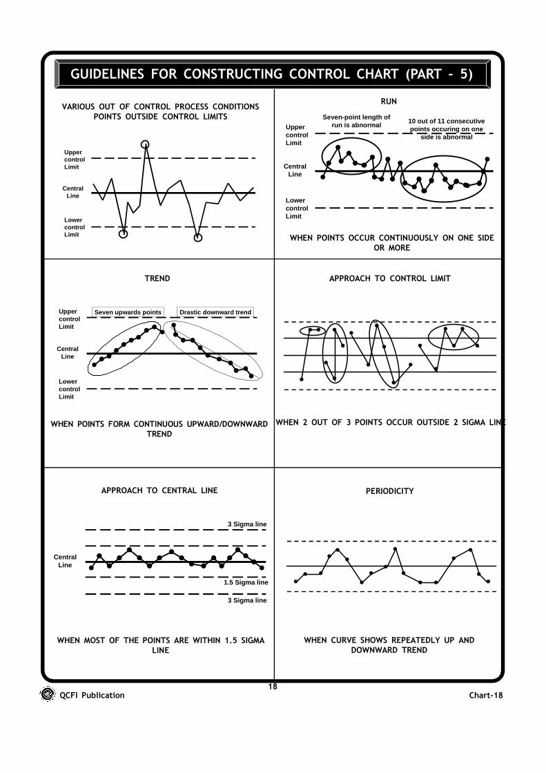
GUIDELINES FOR CONSTRUCTING CONTROL CHART (PART - 5)
CentralLine
UppercontrolLimit
LowercontrolLimit
VARIOUS OUT OF CONTROL PROCESS CONDITIONSPOINTS OUTSIDE CONTROL LIMITS
CentralLine
3 Sigma line
3 Sigma line
1.5 Sigma line
WHEN MOST OF THE POINTS ARE WITHIN 1.5 SIGMALINE
CentralLine
UppercontrolLimit
LowercontrolLimit
Seven-point length ofrun is abnormal
10 out of 11 consecutivepoints occuring on one
side is abnormal
WHEN POINTS OCCUR CONTINUOUSLY ON ONE SIDEOR MORE
CentralLine
UppercontrolLimit
LowercontrolLimit
Seven upwards points Drastic downward trend
WHEN POINTS FORM CONTINUOUS UPWARD/DOWNWARDTREND
•
• •
••
•• •
•
••
••
•
•
•• •
•
WHEN 2 OUT OF 3 POINTS OCCUR OUTSIDE 2 SIGMA LINE
WHEN CURVE SHOWS REPEATEDLY UP ANDDOWNWARD TREND
• • •• •
•
•• •
•
•• •
• •
• •
18
RUN
TREND APPROACH TO CONTROL LIMIT
APPROACH TO CENTRAL LINE PERIODICITY